Rafael Caballero, Mario Rodr´ıguez-Artalejo and Carlos A ...
36
arXiv:1101.2146v1 [cs.PL] 11 Jan 2011 A Generic Scheme for Qualified Constraint Functional Logic Programming ⋆ Technical Report SIC-1-09 Rafael Caballero, Mario Rodr´ ıguez-Artalejo and Carlos A. Romero-D´ ıaz Departamento de Sistemas Inform´ aticos y Computaci´ on, Universidad Complutense, Facultad de Inform´ atica, 28040 Madrid, Spain {rafa,mario}@sip.ucm.es and [email protected] Abstract. Qualification has been recently introduced as a generaliza- tion of uncertainty in the field of Logic Programming. In this report we investigate a more expressive language for First-Order Functional Logic Programming with Constraints and Qualification. We present a Rewrit- ing Logic which characterizes the intended semantics of programs, and a prototype implementation based on a semantically correct program transformation. Potential applications of the resulting language include flexible information retrieval. As a concrete illustration, we show how to write program rules to compute qualified answers for user queries con- cerning the books available in a given library. Keywords: Constraints, Functional Logic Programming, Program Trans- formation, Qualification, Rewriting Logic. 1 Introduction Various extensions of Logic Programming with uncertain reasoning capabilities have been widely investigated during the last 25 years. The recent recollection [21] reviews the evolution of the subject from the viewpoint of a committed researcher. All the proposals in the field replace classical two-valued logic by some kind of many-valued logic with more than two truth values, which are attached to computed answers and interpreted as truth degrees. In a recent work [19,18] we have presented a Qualified Logic Programming scheme QLP(D) parameterized by a qualification domain D, a lattice of so-called qualification values that are attached to computed answers and interpreted as a measure of the satisfaction of certain user expectations. QLP(D)-programs are sets of clauses of the form A α ←− B, where the head A is an atom, the body B is a conjunction of atoms, and α ∈D is called attenuation factor. Intuitively, α measures the maximum confidence placed on an inference performed by the clause. More precisely, any successful application of the clause attaches to the ⋆ Research partially supported by projects MERIT–FORMS (TIN2005-09027-C03- 03), PROMESAS–CAM(S-0505/TIC/0407) and STAMP (TIN2008-06622-C03-01).
Transcript of Rafael Caballero, Mario Rodr´ıguez-Artalejo and Carlos A ...
arX
iv:1
101.
2146
v1 [
cs.P
L]
11
Jan
2011
A Generic Scheme for Qualified
Constraint Functional Logic Programming⋆
Technical Report SIC-1-09
Rafael Caballero, Mario Rodrıguez-Artalejo and Carlos A. Romero-Dıaz
Departamento de Sistemas Informaticos y Computacion, Universidad Complutense,Facultad de Informatica, 28040 Madrid, Spain
rafa,[email protected] and [email protected]
Abstract. Qualification has been recently introduced as a generaliza-tion of uncertainty in the field of Logic Programming. In this report weinvestigate a more expressive language for First-Order Functional LogicProgramming with Constraints and Qualification. We present a Rewrit-ing Logic which characterizes the intended semantics of programs, anda prototype implementation based on a semantically correct programtransformation. Potential applications of the resulting language includeflexible information retrieval. As a concrete illustration, we show how towrite program rules to compute qualified answers for user queries con-cerning the books available in a given library.
Keywords:Constraints, Functional Logic Programming, Program Trans-formation, Qualification, Rewriting Logic.
1 Introduction
Various extensions of Logic Programming with uncertain reasoning capabilitieshave been widely investigated during the last 25 years. The recent recollection[21] reviews the evolution of the subject from the viewpoint of a committedresearcher. All the proposals in the field replace classical two-valued logic bysome kind of many-valued logic with more than two truth values, which areattached to computed answers and interpreted as truth degrees.
In a recent work [19,18] we have presented a Qualified Logic Programmingscheme QLP(D) parameterized by a qualification domain D, a lattice of so-calledqualification values that are attached to computed answers and interpreted as ameasure of the satisfaction of certain user expectations. QLP(D)-programs are
sets of clauses of the form Aα←− B, where the head A is an atom, the body B
is a conjunction of atoms, and α ∈ D is called attenuation factor. Intuitively,α measures the maximum confidence placed on an inference performed by theclause. More precisely, any successful application of the clause attaches to the
⋆ Research partially supported by projects MERIT–FORMS (TIN2005-09027-C03-03), PROMESAS–CAM(S-0505/TIC/0407) and STAMP (TIN2008-06622-C03-01).

2 R. Caballero, M. Rodrıguez-Artalejo and C.A. Romero-Dıaz
head a qualification value which cannot exceed the infimum of αβi ∈ D, whereβi are the qualification values computed for the body atoms and is a so-calledattenuation operator, provided by D.
Uncertain Logic Programming can be expressed by particular instances ofQLP(D), where the user expectation is understood as a lower bound for thetruth degree of the computed answer and D is chosen to formalize a lattice ofnon-classical truth values. Other choices of D can be designed to model otherkinds of user expectations, as e.g. an upper bound for the size of the logical proofunderlying the computed answer. As shown in [4], the QLP(D) scheme is also wellsuited to deal with Uncertain Logic Programming based on similarity relationsin the line of [20]. Therefore, Qualified Logic Programming has a potential forflexible information retrieval applications, where the answers computed for userqueries may match the user expectations only to some degree. As shown in [19],several useful instances of QLP(D) can be conveniently implemented by usingconstraint solving techniques.
In this report we investigate an extension of QLP(D) to a more expres-sive scheme, supporting computation with first-order lazy functions and con-straints. More precisely, we consider the first-order fragment of CFLP(C), ageneric scheme for functional logic programming with constraints over a para-metrically given domain C presented in [13]. We propose an extended schemeQCFLP(D, C) where the additional parameter D stands for a qualification do-main. QCFLP(D, C)-programs are sets of conditional rewrite rules of the form
f(tn)α−→ r ⇐ ∆, where the condition ∆ is a conjunction of C-constraints that
may involve user defined functions, and α ∈ D is an attenuation factor. As inthe logic programming case, α measures the maximum confidence placed on aninference performed by the rule: any successful application of the rule attachesto the computed result a qualification value which cannot exceed the infimumof α βi ∈ D, where βi are the qualification values computed for r and ∆, and is D’s attenuation operator. QLP(D) program clauses can be easily formulatedas a particular case of QCFLP(D, C) program rules.
As far as we know, no related work covers the expressivity of our approach.Guadarrama et al. [8] have proposed to use real arithmetic constraints as animplementation tool for a Fuzzy Prolog, but their language does not supportconstraint programming as such. Starting from the field of natural language pro-cessing, Riezler [15,16] has developed quantitative and probabilistic extensionsof the classical CLP(C) scheme with the aim of computing good parse trees forconstraint logic grammars, but his work bears no relation to functional program-ming. Moreno and Pascual [14] have investigated similarity-based unification inthe context of needed narrowing [1], a narrowing strategy using so-called defini-tional trees that underlies the operational semantics of functional logic languagessuch as Curry [9] and T OY [3], but they use neither constraints nor attenuationfactors and they provide no declarative semantics. The approach of the presentreport is quite different. We work with a class of programs more general andexpressive than the inductively sequential term rewrite systems used in [14], andour results focus on a rewriting logic used to characterize declarative semantics
A Generic Scheme for QCFLP 3
and to prove the correctness of an implementation technique based on a pro-gram transformation. Similarity relations could be easily incorporated to ourscheme by using the techniques presented in [4] for the Logic Programming case.Moreover, the good properties of needed narrowing as a computation model arenot spoiled by our implementation technique, because our program transforma-tion preserves the structure of the definitional trees derived from the user-givenprogram rules.
%% Data types:
type pages, id = inttype title, author, language, genre = [char]data vocabularyLevel = easy | medium | difficult
data readerLevel = basic | intermediate | upper | proficiencydata book = book(id, title, author, language, genre, vocabularyLevel, pages)
%% Simple library, represented as list of books:
library :: [book]library --> [ book(1, "Tintin", "Herge", "French", "Comic", easy, 65),
book(2, "Dune", "F. P. Herbert", "English", "SciFi", medium, 345),
book(3, "Kritik der reinen Vernunft", "Immanuel Kant", "German","Philosophy", difficult, 1011),
book(4, "Beim Hauten der Zwiebel", "Gunter Grass", "German","Biography", medium, 432) ]
%% Auxiliary function for computing list membership:member(B,[]) --> false
member(B,H:_T) --> true <== B == Hmember(B,H:T) --> member(B,T) <== B /= H
%% Functions for getting the explicit attributes of a given book:getId(book(Id,_Title,_Author,_Lang,_Genre,_VocLvl,_Pages)) --> Id
getTitle(book(_Id,Title,_Author,_Lang,_Genre,_VocLvl,_Pages)) --> TitlegetAuthor(book(_Id,_Title,Author,_Lang,_Genre,_VocLvl,_Pages)) --> Author
getLanguage(book(_Id,_Title,_Author,Lang,_Genre,_VocLvl,_Pages)) --> LanggetGenre(book(_Id,_Title,_Author,_Lang,Genre,_VocLvl,_Pages)) --> Genre
getVocabularyLevel(book(_Id,_Title,_Author,_Lang,_Genre,VocLvl,_Pages)) --> VocLvlgetPages(book(_Id,_Title,_Author,_Lang,_Genre,_VocLvl,Pages)) --> Pages
%% Function for guessing the genre of a given book:guessGenre(B) --> getGenre(B)
guessGenre(B) -0.9-> "Fantasy" <== guessGenre(B) == "SciFi"guessGenre(B) -0.8-> "Essay" <== guessGenre(B) == "Philosophy"guessGenre(B) -0.7-> "Essay" <== guessGenre(B) == "Biography"
guessGenre(B) -0.7-> "Adventure" <== guessGenre(B) == "Fantasy"
%% Function for guessing the reader level of a given book:guessReaderLevel(B) --> basic <== getVocabularyLevel(B) == easy, getPages(B) < 50
guessReaderLevel(B) -0.8-> intermediate <== getVocabularyLevel(B) == easy, getPages(B) >= 50guessReaderLevel(B) -0.9-> basic <== guessGenre(B) == "Children"guessReaderLevel(B) -0.9-> proficiency <== getVocabularyLevel(B) == difficult,
getPages(B) >= 200guessReaderLevel(B) -0.8-> upper <== getVocabularyLevel(B) == difficult, getPages(B) < 200
guessReaderLevel(B) -0.8-> intermediate <== getVocabularyLevel(B) == mediumguessReaderLevel(B) -0.7-> upper <== getVocabularyLevel(B) == medium
%% Function for answering a particular kind of user queries:search(Language,Genre,Level) --> getId(B) <== member(B,library),
getLanguage(B) == Language,guessReaderLevel(B) == Level,
guessGenre(B) == Genre
Fig. 1. Library with books in different languages

4 R. Caballero, M. Rodrıguez-Artalejo and C.A. Romero-Dıaz
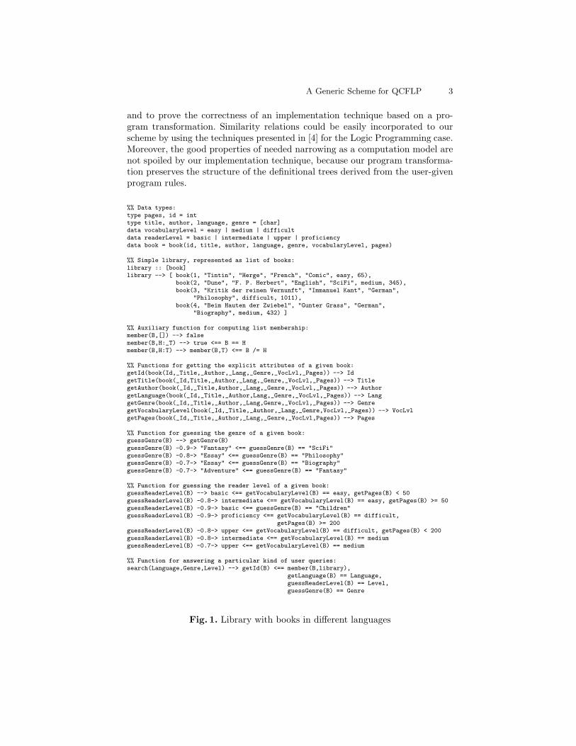
Figure 1 shows a small set of QCFLP(U ,R) program rules, called the libraryprogram in the rest of the report. The concrete syntax is inspired by the func-tional logic language T OY , but the ideas and results of this report could be alsoapplied to Curry and other similar languages. In this example, U stands for aparticular qualification domain which supports uncertain truth values in the realinterval [0, 1], while R stands for a particular constraint domain which supportsarithmetic constraints over the real numbers; see Section 2 for more details.
The program rules are intended to encode expert knowledge for computingqualified answers to user queries concerning the books available in a simplifiedlibrary, represented as a list of objects of type book. The various get func-tions extract the explicit values of book attributes. Functions guessGenre andguessReaderLevel infer information by performing qualified inferences, relyingon analogies between different genres and heuristic rules to estimate reader lev-els on the basis of other features of a given book, respectively. Some programrules, as e.g. those of the auxiliary function member, have attached no explicitattenuation factor. By convention, this is understood as the implicit attach-ment of the attenuation factor 1.0, the top value of U . For any instance of theQCFLP(D, C) scheme, a similar convention allows to view CFLP(C)-programrules as QCFLP(D, C)-program rules whose attached qualification is optimal.
The last rule for function search encodes a method for computing qualifiedanswers to a particular kind of user queries. Therefore, the queries can be formu-lated as goals to be solved by the program fragment. For instance, answering thequery of a user who wants to find a book of genre "Essay", language "German"and user level intermediate with a certainty degree of at least 0.65 can beformulated as the goal:
(search("German","Essay",intermediate) == R) # W | W >= 0.65
The techniques presented in Section 4 can be used to translate the QCFLP(U ,R)program rules and goal into the CFLP(R) language, which is implemented inthe T OY system. Solving the translated goal in T OY computes the answerR 7→ 40.65 ≤W,W ≤ 0.7, ensuring that the library book with id 4 satisfiesthe query’s requirements with any certainty degree in the interval [0.65,0.7], inparticular 0.7. The computation uses the 4th program rule of guessGenre toobtain "Essay" as the book’s genre with qualification 0.7, and the 6th programrule of guessReaderLevel to obtain intermediate as the reader level withqualification 0.8.
The rest of the report is organized as follows. In Section 2 we recall knownproposals concerning qualification and constraint domains, and we introduce atechnical notion needed to relate both kinds of domains for the purposes of thisreport. In Section 3 we present the generic scheme QCFLP(D, C) announced inthis introduction, and we formalize a special Rewriting Logic which characterizesthe declarative semantics of QCFLP(D, C)-programs. In Section 4 we present asemantically correct program transformation converting QCFLP(D, C) programsand goals into the qualification-free CFLP(C) programming scheme, which issupported by existing systems such as T OY . Section 5 concludes and points tosome lines of planned future work.

A Generic Scheme for QCFLP 5
2 Qualification and Constraint Domains
Qualification Domains were introduced in [19]. Their intended use has been al-ready explained in the Introduction. In this section we recall and slightly improvetheir axiomatic definition.
Definition 1 (Qualification Domains). A Qualification Domain is any struc-ture D = 〈D,P,b, t, 〉 verifying the following requirements:
1. D, noted as DD when convenient, is a set of elements called qualificationvalues.
2. 〈D,P,b, t〉 is a lattice with extreme points b and t w.r.t. the partial orderingP. For given elements d, e ∈ D, we write d ⊓ e for the greatest lower bound(glb) of d and e, and d ⊔ e for the least upper bound (lub) of d and e. Wealso write d ⊳ e as abbreviation for d P e ∧ d 6= e.
3. : D×D −→ D, called attenuation operation, verifies the following axioms:(a) is associative, commutative and monotonic w.r.t. P.(b) ∀d ∈ D : d t = d.(c) ∀d, e ∈ D \ b, t : d e ⊳ e.(d) ∀d, e1, e2 ∈ D : d (e1 ⊓ e2) = d e1 ⊓ d e2. ⊓⊔
As an easy consequence of the previous definition one can prove the followingproposition. 1
Proposition 1 (Additional properties of qualification domains). Anyqualification domain D satisfies the following properties:
1. ∀d, e ∈ D : d e P e.2. ∀d ∈ D : d b = b.
Proof. Since t is the top element of the lattice, we know d P t for any d ∈ D.As is monotonic w.r.t. P, d e P t e also holds for any e ∈ D which, dueto commutativity and axiom (b) of , yields d e P e. Therefore 1 . holds. Now,taking e = b, one has d b P b which implies d b = b as b is the bottomelement of the lattice. Hence 2 . also holds. ⊓⊔
The examples in this report will use a particular qualification domain Uwhose values represent certainty degrees in the sense of fuzzy logic. Formally,U = 〈U,≤, 0, 1,×〉, where U = [0, 1] = d ∈ R | 0 ≤ d ≤ 1, ≤ is the usualnumerical ordering, and × is the multiplication operation. In this domain, thebottom and top elements are b = 0 and t = 1, and the infimum of a finiteS ⊆ U is the minimum value min(S), understood as 1 if S = ∅. The class ofqualification domains is closed under cartesian products. For a proof of this factand other examples of qualification domains, the reader is referred to [19,18].
Constraint domains are used in Constraint Logic Programming and its ex-tensions as a tool to provide data values, primitive operations and constraints
1 The authors are thankful to G. Gerla for pointing out this fact.

6 R. Caballero, M. Rodrıguez-Artalejo and C.A. Romero-Dıaz
tailored to domain-oriented applications. Various formalizations of this notionare known. In this report, constraint domains are related to signatures of theform Σ = 〈DC,PF,DF 〉 where DC =
⋃n∈N
DCn, PF =⋃
n∈NPFn and
DF =⋃
n∈NDFn are mutually disjoint sets of data constructor symbols, primi-
tive function symbols and defined function symbols, respectively, ranked by ari-ties. Given a signatureΣ, a symbol ⊥ to note the undefined value, a set B of basicvalues u and a countably infinite set Var of variables X , we define the notionslisted below, where on abbreviates the n-tuple of syntactic objects o1, . . . , on.
– Expressions e ∈ Exp⊥(Σ,B,Var) have the syntax e ::= ⊥|X |u|h(en), whereh ∈ DCn ∪ PFn ∪DFn. In the case n = 0, h(en) is written simply as h.
– Constructor Terms t ∈ Term⊥(Σ,B,Var) have the syntax e ::= ⊥|X |u|c(tn),where c ∈ DCn. They will be called just terms in the sequel.
– Total Expressions e ∈ Exp(Σ,B,Var) and Total Terms t ∈ Term(Σ,B,Var)have a similar syntax, with the ⊥ case omitted.
– An expression or term (total or not) is called ground iff it includes no oc-currences of variables. Exp⊥(Σ,B) stands for the set of all ground expres-sions. The notations Term⊥(Σ,B), Exp(Σ,B) and Term(Σ,B) have a sim-ilar meaning.
– We note as ⊑ the information ordering, defined as the least partial orderingover Exp⊥(Σ,B,Var) compatible with contexts and verifying ⊥ ⊑ e for alle ∈ Exp⊥(Σ,B,Var).
– Substitutions are defined as mappings σ : Var → Term⊥(Σ,B,Var) assigningnot necessarily total terms to variables. They can be represented as sets ofbindings X 7→ t and extended to act over other syntactic objects o. Thedomain vdom(σ) and variable range vran(σ) are defined in the usual way.We will write oσ for the result of applying σ to o. The composition σσ′ oftwo substitutions is such that o(σσ′) equals (oσ)σ′.
By adapting the definition found in Section 2.2 of [13] to a first-order setting,we obtain: 2
Definition 2 (Constraint Domains). A Constraint Domain of signature Σis any algebraic structure of the form C = 〈C, pC | p ∈ PF〉 such that:
1. The carrier set C is Term⊥(Σ,B) for a certain set B of basic values. Whenconvenient, we note B and C as BC and CC , respectively.
2. pC ⊆ Cn × C, written simply as pC ⊆ C in the case n = 0, is called theinterpretation of p in C. We will write pC(tn) → t (or simply pC → t ifn = 0) to indicate that (tn, t) ∈ pC.
3. Each primitive interpretation pC has monotonic and radical behavior w.r.t.the information ordering ⊑. More precisely:(a) Monotonicity: For all p ∈ PFn, pC(tn) → t behaves monotonically
w.r.t. the arguments tn and antimonotonically w.r.t. the result t. For-mally: For all tn, t′n, t, t
′ ∈ C such that pC(tn)→ t, tn ⊑ t′n and t ⊒ t′,pC(t′n)→ t′ also holds.
2 We slightly modify the statement of the radicality property, rendering it simpler thanin [13] but sufficient for practical purposes.

A Generic Scheme for QCFLP 7
(b) Radicality: For all p ∈ PFn, as soon as the arguments given to pC haveenough information to return a result other than ⊥, the same argumentssuffice already for returning a simple total result. Formally: For all tn, t ∈C, if pC(tn)→ t then t = ⊥ or else t ∈ B ∪DC0.
Note that symbols h ∈ DC ∪DF are given no interpretation in C. As we willsee in Section 3, symbols in c ∈ DC are interpreted as free constructors, and theinterpretation of symbols f ∈ DF is program-dependent. We assume that anysignature Σ includes two nullary constructors true and false for the booleanvalues, and a binary symbol == ∈ PF 2 used in infix notation and interpretedas strict equality; see [13] for details. For the examples in this report we willuse a constraint domain R whose set of basic elements is CR = R and whoseprimitives functions correspond to the usual arithmetic operations +,×, . . . andthe usual boolean-valued comparison operations ≤, <, . . . over R. Other usefulinstances of constraint domains can be found in [13].
Atomic constraints over C have the form p(en) == v 3 with p ∈ PFn,ei ∈ Exp⊥(Σ,B,Var) and v ∈ Var ∪DC
0 ∪BC . Atomic constraints of the formp(en) == true are abbreviated as p(en). In particular, (e1 == e2) == true isabbreviated as e1 == e2. Atomic constraints of the form (e1 == e2) == falseare abbreviated as e1 /= e2.
Compound constraints are built from atomic constraints using logical con-junction, existential quantification, and sometimes other logical operations. Con-straints without occurrences of symbols f ∈ DF are called primitive. We willnote atomic constraints as δ, sets of atomic constraints as ∆, atomic primitiveconstraints as π, and sets of atomic primitive constraints as Π . When interpret-ing set of constraints, we will treat them as the conjunction of their members.
Ground substitutions η such that Xη ∈ Term⊥(Σ,B) for all X ∈ vdom(η)are called variable valuations over C. The set of all possible variable valuations isnoted ValC . The solution set SolC(Π) ⊆ ValC includes as members those valua-tions η such that πη is true in C for all π ∈ Π ; see [13] for a formal definition. Incase that SolC(Π) = ∅ we say that Π is unsatisfiable and we write UnsatC(Π).In case that SolC(Π) ⊆ SolC(π) we say that π is entailed by Π in C and we writeΠ |=C π. Note that the notions defined in this paragraph only make sense forprimitive constraints.
In this report we are interested in pairs consisting of a qualification domainand a constraint domain that are related in the following technical sense:
Definition 3 (Expressing D in C). A qualification domain D with carrier setDD is expressible in a constraint domain C with carrier set CC if DD \b ⊆ CC
and the two following requirements are satisfied:
1. There is a primitive C-constraint qVal(X) depending on the variable X, suchthat SolC(qVal(X)) = η ∈ ValC | η(X) ∈ DD \ b.
2. There is a primitive C-constraint qBound(X,Y, Z) depending on the variablesX, Y , Z, such that any η ∈ ValC such that η(X), η(Y ), η(Z) ∈ DD \ bverifies η ∈ SolC(qBound(X,Y, Z))⇐⇒ η(X) P η(Y ) η(Z). ⊓⊔
3 Written as p(en) →! v in [13].

8 R. Caballero, M. Rodrıguez-Artalejo and C.A. Romero-Dıaz
Intuitively, qBound(X,Y, Z) encodes the D-statement X P Y Z as a C-constraint. As convenient notations, we will write pX P Y Zq, pX P Y q andpX Q Y q in place of qBound(X,Y, Z), qBound(X, t, Y ) and qBound(Y, t, X),respectively. In the sequel, C-constraints of the form pκq are called qualificationconstraints, and Ω is used as notation for sets of qualification constraints. Wealso write ValD for the set of all µ ∈ ValC such that Xµ ∈ DD \ b for allX ∈ vdom(µ), called D-valuations.
Note that U can be expressed in R, because DU \ 0 = (0, 1] ⊆ R ⊆ CR,qVal(X) can be built as the R-constraint 0 < X ∧ X ≤ 1 and pX P Y Zqcan be built as the R-constraint X ≤ Y × Z. Other instances of qualificationdomains presented in [19] are also expressible in R.
3 A Qualified Declarative Programming Scheme
In this section we present the scheme QCFLP(D, C) announced in the Introduc-tion, and we develop alternative characterizations of its declarative semanticsusing an interpretation transformer and a rewriting logic. The parameters Dand C respectively stand for a qualification domain and a constraint domainwith certain signature Σ. By convention, we only allow those instances of thescheme verifying that D is expressible in C in the sense of Definition 3. Forexample, QCFLP(U ,R) is an allowed instance.
Technically, the results presented here extend similar ones known for theCFLP(C) sheme [13], omitting higher-order functions and adding a suitable treat-ment of qualifications. In particular, the qc-interpretations for QCFLP(D, C)-programs are a natural extension of the c-interpretations for CFLP(C)-programsintroduced in [13]. In turn, these were inspired by the π-interpretations for theCLP(C) scheme proposed by Dore, Gabbrielli and Levi [7,6].
3.1 Programs, Interpretations and Models
A QCFLP(D, C)-program is a set P of program rules. A program rule has the
form f(tn)α−→ r ⇐ ∆ where f ∈ DFn, tn is a lineal sequence of Σ-terms,
α ∈ DD \b is an attenuation factor, r is a Σ-expression and ∆ is a sequence ofatomic C-constraints δj (1 ≤ j ≤ m), interpreted as conjunction. The undefinedsymbol ⊥ is not allowed to occur in program rules.
The library program shown in Figure 1 is an example of QCFLP(U ,R)-program. Leaving aside the attenuation factors, this is clearly not a conflu-ent conditional term rewriting system. Certain program rules, as e.g. those forguessGenre, are intended to specify the behavior of non-deterministic functions.As argued elsewhere [17], the semantics of non-deterministic functions for thepurposes of Functional Logic Programming is not suitably described by ordinaryrewriting. Inspired by the approach in [13], we will overcome this difficulty bydesigning special inference mechanisms to derive semantically meaningful state-ments from programs. The kind of statements that we will consider are definedbelow:

A Generic Scheme for QCFLP 9
Definition 4 (qc-Statements). Assume partial Σ-expression e, partial Σ-terms t, t′, tn, a qualification value d ∈ DD \b, an atomic C-constraint δ and afinite set of atomic primitive C-constraints Π. A qualified constrained statement(briefly, qc-statement) ϕ must have one of the following two forms:
1. qc-production (e→ t)♯d⇐ Π. Such a qc-statement is called trivial iff eithert is ⊥ or else UnsatC(Π). Its intuitive meaning is that a rewrite sequencee→∗ t′ using program rules and with attached qualification value d is allowedin our intended semantics for some t′ ⊒ t, under the assumption that Πholds. By convention, qc-productions of the form (f(tn) → t)♯d ⇐ Π withf ∈ DFn are called qc-facts.
2. qc-atom δ♯d ⇐ Π. Such a qc-statement is called trivial iff UnsatC(Π). Itsintuitive meaning is that δ is entailed by the program rules with attachedqualification value d, under the assumption that Π holds. ⊓⊔
Our semantics will use program interpretations defined as sets of qc-facts withcertain closure properties. As an auxiliary tool we need the following technicalnotion:
Definition 5 ((D, C)-Entailment). Given two qc-statements ϕ and ϕ′, we saythat ϕ (D, C)-entails ϕ′ (in symbols, ϕ <D,C ϕ
′) iff one of the following two caseshold:
1. ϕ = (e→ t)♯d⇐ Π, ϕ′ = (e′ → t′)♯d′ ⇐ Π ′, and there is some substitutionσ such that Π ′ |=C Πσ, d Q d′, eσ ⊑ e′ and tσ ⊒ t′.
2. ϕ = δ♯d ⇐ Π, ϕ′ = δ′♯d′ ⇐ Π ′, and there is some substitution σ such thatΠ ′ |=C Πσ, d Q d′, δσ ⊑ δ′. ⊓⊔
The intended meaning of ϕ <D,C ϕ′ is that ϕ′ follows from ϕ, regardlessof the interpretation of the defined function symbols f ∈ DF occurring in ϕ,ϕ′. Intuitively, this is the case because the interpretations of defined functionsymbols are expected to satisfy the monotonicity properties stated for the caseof primitive function symbols in Definition 2. The following example may helpto understand the idea:
Example 1 ((U ,R)-entailment). Let ϕ, ϕ′ be defined as:
ϕ : (f(X :Xs)→ Xs)♯0.8⇐ X ×X 6= 0ϕ′ : (f(A : (B : [ ])) → ⊥ :⊥)♯0.7⇐ A < 0
Then ϕ <U ,R ϕ′ with σ = X 7→ A, Xs 7→ B :⊥ because:
– Π ′ |=R Πσ, since Π ′ = A < 0, Πσ = X ×X 6= 0σ = A×A 6= 0, andA×A 6= 0 is entailed by A < 0 in R.
– d Q d′ holds in U , since d = 0.8 ≥ 0.7 = d′.– eσ ⊑ e′, since eσ = f(X :Xs)σ = f(A : (B :⊥)) ⊑ f(A : (B : [ ])) = e′.– tσ ⊒ t′, since tσ = Xsσ = B :⊥ ⊒ ⊥ :⊥ = t′. ⊓⊔
Now we can define program interpretations as follows:

10 R. Caballero, M. Rodrıguez-Artalejo and C.A. Romero-Dıaz
Definition 6 (qc-Interpretations). A qualified constrained interpretation (orqc-interpretation) over D and C is a set I of qc-facts including all trivial andentailed qc-facts. In other words, a set I of qc-facts such that clD,C(I) ⊆ I,where the closure over D and C of I is defined as:
clD,C(I) =def ϕ | ϕ trivial ∪ ϕ′ | ϕ <D,C ϕ′ for some ϕ ∈ I .
We write IntD,C for the set of all qc-interpretations over D and C.
QTIϕ
if ϕ is a trivial qc-statement.
QRR(v → v)♯d⇐ Π
if v ∈ Var ∪BC and d ∈ DD \ b.
QDC( (ei → ti)♯di ⇐ Π )i=1...n
(c(en) → c(tn))♯d⇐ Π
if c ∈ DCn and d ∈ DD \ bverifies d P di (1 ≤ i ≤ n).
QDFI
( (ei → ti)♯di ⇐ Π )i=1...n
(f(en) → t)♯d⇐ Π
if f ∈ DFn, non-trivial ((f(tn) → t)♯d0 ⇐ Π) ∈ Iand d ∈ DD \ b verifies d P di (0 ≤ i ≤ n).
QPF( (ei → ti)♯di ⇐ Π )i=1...n
(p(en) → v)♯d⇐ Πif p ∈ PFn, v ∈ Var ∪DC0 ∪BC ,
Π |=C p(tn) → v and d ∈ DD \ b verifies d P di (1 ≤ i ≤ n).
QAC( (ei → ti)♯di ⇐ Π )i=1...n
(p(en) == v)♯d⇐ Πif p ∈ PFn, v ∈ Var ∪DC0 ∪ BC,
Π |=C p(tn) == v and d ∈ DD \ b verifies d P di (1 ≤ i ≤ n).
Fig. 2. Qualified Constrained Rewriting Logic for Interpretations
Given a qc-interpretation I, the inference rules displayed in Fig. 2 are usedto derive qc-statements from the qc-facts belonging to I. The inference systemconsisting of these rules is called Qualified Constrained Rewriting Logic for In-terpretations and noted as I-QCRWL(D, C). The notation I ⊢⊢D,C ϕ is used toindicate that ϕ can be derived from I in I-QCRWL(D, C). By convention, weagree that no other inference rule is used whenever QTI is applicable. Therefore,trivial qc-statements can only be inferred by rule QTI. As usual in formal infer-ence systems, I-QCRWL(D, C) proofs can be represented as trees whose nodescorrespond to inference steps.
A Generic Scheme for QCFLP 11
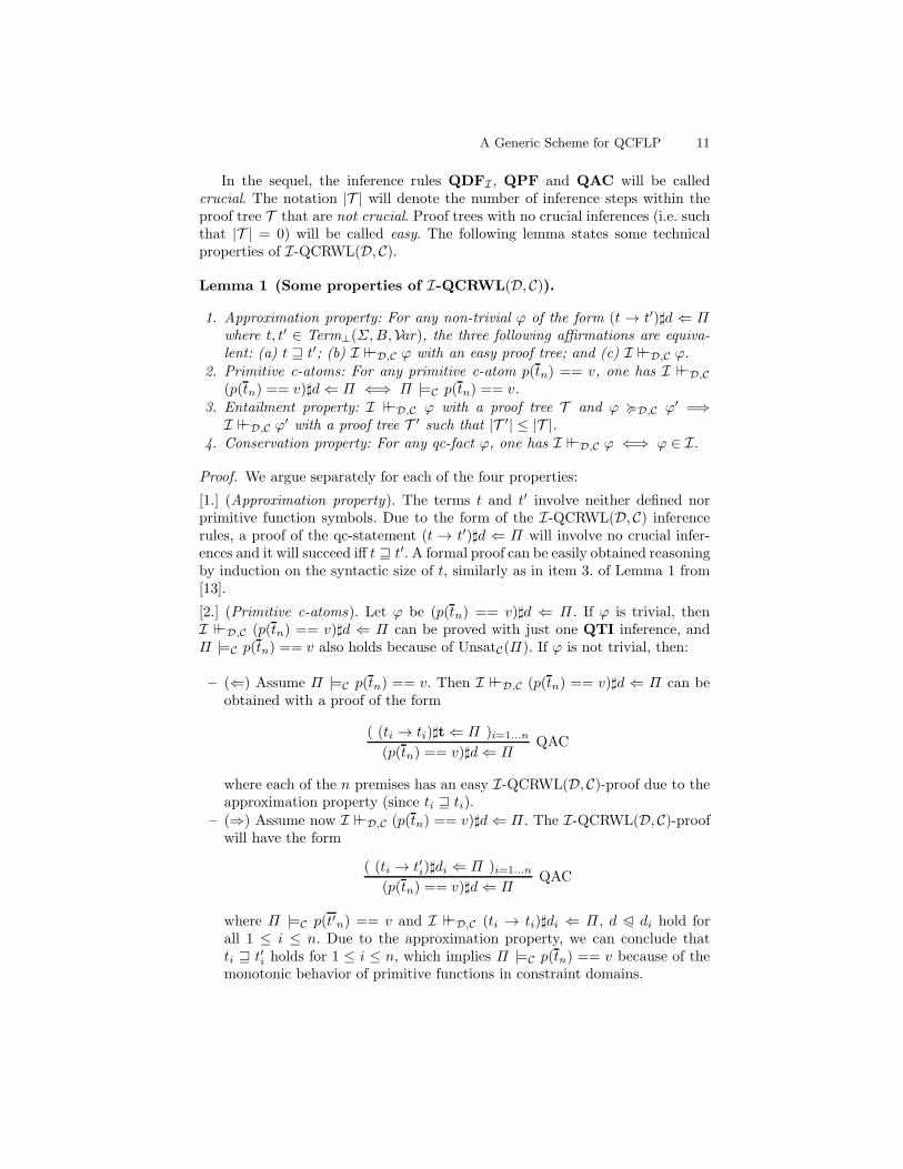
In the sequel, the inference rules QDFI , QPF and QAC will be calledcrucial. The notation |T | will denote the number of inference steps within theproof tree T that are not crucial. Proof trees with no crucial inferences (i.e. suchthat |T | = 0) will be called easy. The following lemma states some technicalproperties of I-QCRWL(D, C).
Lemma 1 (Some properties of I-QCRWL(D, C)).
1. Approximation property: For any non-trivial ϕ of the form (t → t′)♯d ⇐ Πwhere t, t′ ∈ Term⊥(Σ,B,Var), the three following affirmations are equiva-lent: (a) t ⊒ t′; (b) I ⊢⊢D,C ϕ with an easy proof tree; and (c) I ⊢⊢D,C ϕ.
2. Primitive c-atoms: For any primitive c-atom p(tn) == v, one has I ⊢⊢D,C
(p(tn) == v)♯d⇐ Π ⇐⇒ Π |=C p(tn) == v.3. Entailment property: I ⊢⊢D,C ϕ with a proof tree T and ϕ <D,C ϕ′ =⇒I ⊢⊢D,C ϕ
′ with a proof tree T ′ such that |T ′| ≤ |T |.4. Conservation property: For any qc-fact ϕ, one has I ⊢⊢D,C ϕ ⇐⇒ ϕ ∈ I.
Proof. We argue separately for each of the four properties:
[1.] (Approximation property). The terms t and t′ involve neither defined norprimitive function symbols. Due to the form of the I-QCRWL(D, C) inferencerules, a proof of the qc-statement (t → t′)♯d ⇐ Π will involve no crucial infer-ences and it will succeed iff t ⊒ t′. A formal proof can be easily obtained reasoningby induction on the syntactic size of t, similarly as in item 3. of Lemma 1 from[13].
[2.] (Primitive c-atoms). Let ϕ be (p(tn) == v)♯d ⇐ Π . If ϕ is trivial, thenI ⊢⊢D,C (p(tn) == v)♯d ⇐ Π can be proved with just one QTI inference, andΠ |=C p(tn) == v also holds because of UnsatC(Π). If ϕ is not trivial, then:
– (⇐) Assume Π |=C p(tn) == v. Then I ⊢⊢D,C (p(tn) == v)♯d ⇐ Π can beobtained with a proof of the form
( (ti → ti)♯t⇐ Π )i=1...n
(p(tn) == v)♯d⇐ ΠQAC
where each of the n premises has an easy I-QCRWL(D, C)-proof due to theapproximation property (since ti ⊒ ti).
– (⇒) Assume now I ⊢⊢D,C (p(tn) == v)♯d⇐ Π . The I-QCRWL(D, C)-proofwill have the form
( (ti → t′i)♯di ⇐ Π )i=1...n
(p(tn) == v)♯d⇐ ΠQAC
where Π |=C p(t′n) == v and I ⊢⊢D,C (ti → ti)♯di ⇐ Π , d P di hold forall 1 ≤ i ≤ n. Due to the approximation property, we can conclude thatti ⊒ t′i holds for 1 ≤ i ≤ n, which implies Π |=C p(tn) == v because of themonotonic behavior of primitive functions in constraint domains.
12 R. Caballero, M. Rodrıguez-Artalejo and C.A. Romero-Dıaz
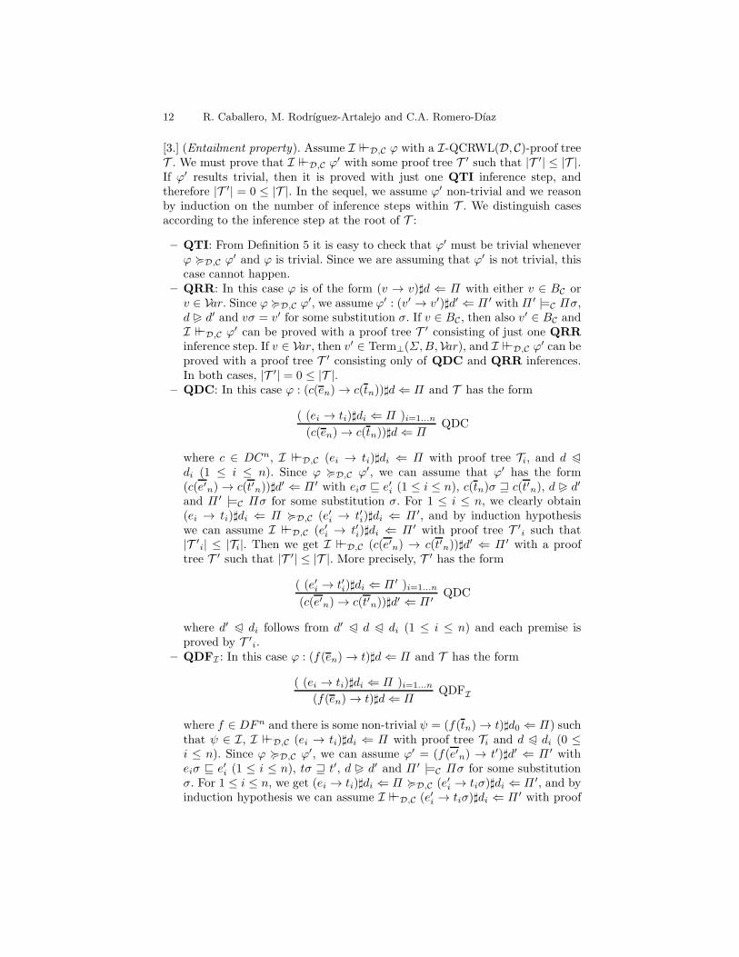
[3.] (Entailment property). Assume I ⊢⊢D,C ϕ with a I-QCRWL(D, C)-proof treeT . We must prove that I ⊢⊢D,C ϕ
′ with some proof tree T ′ such that |T ′| ≤ |T |.If ϕ′ results trivial, then it is proved with just one QTI inference step, andtherefore |T ′| = 0 ≤ |T |. In the sequel, we assume ϕ′ non-trivial and we reasonby induction on the number of inference steps within T . We distinguish casesaccording to the inference step at the root of T :
– QTI: From Definition 5 it is easy to check that ϕ′ must be trivial wheneverϕ <D,C ϕ
′ and ϕ is trivial. Since we are assuming that ϕ′ is not trivial, thiscase cannot happen.
– QRR: In this case ϕ is of the form (v → v)♯d ⇐ Π with either v ∈ BC orv ∈ Var. Since ϕ <D,C ϕ
′, we assume ϕ′ : (v′ → v′)♯d′ ⇐ Π ′ with Π ′ |=C Πσ,d Q d′ and vσ = v′ for some substitution σ. If v ∈ BC , then also v′ ∈ BC andI ⊢⊢D,C ϕ
′ can be proved with a proof tree T ′ consisting of just one QRRinference step. If v ∈ Var, then v′ ∈ Term⊥(Σ,B,Var), and I ⊢⊢D,C ϕ
′ can beproved with a proof tree T ′ consisting only of QDC and QRR inferences.In both cases, |T ′| = 0 ≤ |T |.
– QDC: In this case ϕ : (c(en)→ c(tn))♯d⇐ Π and T has the form
( (ei → ti)♯di ⇐ Π )i=1...n
(c(en)→ c(tn))♯d⇐ ΠQDC
where c ∈ DCn, I ⊢⊢D,C (ei → ti)♯di ⇐ Π with proof tree Ti, and d Pdi (1 ≤ i ≤ n). Since ϕ <D,C ϕ′, we can assume that ϕ′ has the form(c(e′n)→ c(t′n))♯d
′ ⇐ Π ′ with eiσ ⊑ e′i (1 ≤ i ≤ n), c(tn)σ ⊒ c(t′n), d Q d′
and Π ′ |=C Πσ for some substitution σ. For 1 ≤ i ≤ n, we clearly obtain(ei → ti)♯di ⇐ Π <D,C (e′i → t′i)♯di ⇐ Π ′, and by induction hypothesiswe can assume I ⊢⊢D,C (e′i → t′i)♯di ⇐ Π ′ with proof tree T ′
i such that|T ′
i| ≤ |Ti|. Then we get I ⊢⊢D,C (c(e′n) → c(t′n))♯d′ ⇐ Π ′ with a proof
tree T ′ such that |T ′| ≤ |T |. More precisely, T ′ has the form
( (e′i → t′i)♯di ⇐ Π ′ )i=1...n
(c(e′n)→ c(t′n))♯d′ ⇐ Π ′QDC
where d′ P di follows from d′ P d P di (1 ≤ i ≤ n) and each premise isproved by T ′
i.– QDFI : In this case ϕ : (f(en)→ t)♯d⇐ Π and T has the form
( (ei → ti)♯di ⇐ Π )i=1...n
(f(en)→ t)♯d⇐ ΠQDFI
where f ∈ DFn and there is some non-trivial ψ = (f(tn)→ t)♯d0 ⇐ Π) suchthat ψ ∈ I, I ⊢⊢D,C (ei → ti)♯di ⇐ Π with proof tree Ti and d P di (0 ≤i ≤ n). Since ϕ <D,C ϕ
′, we can assume ϕ′ = (f(e′n) → t′)♯d′ ⇐ Π ′ witheiσ ⊑ e′i (1 ≤ i ≤ n), tσ ⊒ t′, d Q d′ and Π ′ |=C Πσ for some substitutionσ. For 1 ≤ i ≤ n, we get (ei → ti)♯di ⇐ Π <D,C (e′i → tiσ)♯di ⇐ Π ′, and byinduction hypothesis we can assume I ⊢⊢D,C (e′i → tiσ)♯di ⇐ Π ′ with proof

A Generic Scheme for QCFLP 13
tree T ′i such that |T ′
i| ≤ |Ti|. Consider now ψ′ = ((f(tn)σ → t′)♯d0 ⇐ Π ′).Clearly, ψ <D,C ψ
′ and therefore ψ′ ∈ I because I is closed under (D, C)-entailment. Using this ψ′ we get I ⊢⊢D,C (f(e′n)→ t′)♯d′ ⇐ Π ′ with a prooftree T ′ such that |T ′| ≤ |T |. More precisely, T ′ has the form
( (e′i → tiσ)♯di ⇐ Π ′ )i=1...n
(f(e′n)→ t′)♯d′ ⇐ Π ′QDFI
where d′ P di follows from d′ P d P di (0 ≤ i ≤ n) and each premise isproved by T ′
i.
– QPF: In this case ϕ : (p(en)→ v)♯d⇐ Π and T has the form
( (ei → ti)♯di ⇐ Π )i=1...n
(p(en)→ v)♯d⇐ ΠQPF
where p ∈ PFn, v ∈ Var ∪DC0 ∪BC , Π |=C p(tn)→ v, d P di and I ⊢⊢D,C
(ei → ti)♯di ⇐ Π with proof tree Ti (1 ≤ i ≤ n). Since ϕ <D,C ϕ′, we can
assume ϕ′ to be of the form (p(e′n)→ v′)♯d′ ⇐ Π ′ with eiσ ⊑ e′i (1 ≤ i ≤ n),vσ ⊒ v′, d Q d′ and Π ′ |=C Πσ for some substitution σ. For 1 ≤ i ≤ n, weget (ei → ti)♯di ⇐ Π <D,C (e′i → tiσ)♯di ⇐ Π ′, and by induction hypothesiswe can assume I ⊢⊢D,C (e′i → tiσ)♯di ⇐ Π ′ with proof tree T ′
i such that|T ′
i| ≤ |Ti|. Moreover, we can also assume v′ ∈ Var∪DC0∪BC because p is aprimitive function symbol and ϕ′ is not trivial. From v, v′ ∈ Var∪DC0 ∪BC
and vσ ⊒ v′ we can conclude that vσ = v′. Then, from Π |=C p(tn) → vand Π ′ |=C Πσ we can deduce Π ′ |=C p(tn)σ → v′. Putting everythingtogether, we get I ⊢⊢D,C (p(e′n) → v′)♯d′ ⇐ Π ′ with a proof tree T ′ suchthat |T ′| ≤ |T |. More precisely, T ′ has the form
( (e′i → tiσ)♯di ⇐ Π ′ )i=1...n
(p(e′n)→ v′)♯d′ ⇐ Π ′QPF
where d′ P di follows from d′ P d P di (1 ≤ i ≤ n) and each premise isproved by T ′
i.– QAC: Similar to the case for QPF.
[4.] (Conservation property). Assume ϕ : (f(tn) → t)♯d ⇐ Π . In the case thatϕ is a trivial qc-fact, it is true by definition of qc-interpretation that ϕ ∈ I,and I ⊢⊢D,C ϕ follows by rule QTI. Therefore the property is satisfied for trivialqc-facts. If ϕ is not trivial, we prove each implication as follows:
– (⇐) Assume ϕ ∈ I. Then I ⊢⊢D,C ϕ with a I-QCRWL(D, C)-proof tree ofthe form:
( (ti → ti)♯t⇐ Π )i=1...n
(f(tn)→ t)♯d⇐ ΠQDFI using ϕ ∈ I
where each premise has an easy I-QCRWL(D, C)-proof tree due to the ap-proximation property, and d P d, t hold trivially.

14 R. Caballero, M. Rodrıguez-Artalejo and C.A. Romero-Dıaz
– (⇒) Assume I ⊢⊢D,C ϕ. As ϕ is not trivial, there is a I-QCRWL(D, C)-prooftree of the form:
( (ti → t′i)♯di ⇐ Π )i=1...n
(f(tn)→ t)♯d⇐ ΠQDFI using ϕ′ = (f(t′n)→ t)♯d′ ⇐ Π) ∈ I
where d P d′, di and I ⊢⊢D,C (ti → t′i)♯di ⇐ Π (1 ≤ i ≤ n). For each1 ≤ i ≤ n, we claim that t′i ⊑ ti. If t
′i = ⊥ the claim is trivial. If t′i 6= ⊥, then
(ti → t′i)♯di ⇐ Π is a non-trivial qc-production and the claim follows fromI ⊢⊢D,C (ti → t′i)♯di ⇐ Π and the approximation property. Now, the claimtogether with Π |=C Π , d′ Q d and t ⊒ t yields ϕ′ <D,C ϕ. Since ϕ
′ ∈ I andI is closed under (D, C)-entailment, we can conclude that ϕ ∈ I. ⊓⊔
Next, we can define program models and semantic consequence, adaptingideas from the so-called strong semantics of [13]. 4
Definition 7 (Models and semantic consequence). Let a QCFLP(D, C)-program P be given.
1. A qc-interpretation I is a model of Rl : (f(tn)α−→ r ⇐ δm) ∈ P (in
symbols, I |=D,C Rl) iff for every substitution θ, for every set of atomicprimitive C-constraints Π, for every c-term t ∈ Term⊥(Σ,B,Var) and forall d, d0, . . . , dm ∈ DD \ b such that I ⊢⊢D,C δiθ♯d
′i ⇐ Π (1 ≤ i ≤ m),
I ⊢⊢D,C (rθ → t)♯d′0 ⇐ Π and d P α di (0 ≤ i ≤ m), one has ((f(tn)θ →t)♯d⇐ Π) ∈ I.
2. A qc-interpretation I is a model of P (in symbols, I |=D,C P) iff I is amodel of every program rule belonging to P.
3. A qc-statement ϕ is a semantic consequence of P (in symbols, P |=D,C ϕ)iff I ⊢⊢D,C ϕ holds for every qc-interpretation I such that I |=D,C P. ⊓⊔
3.2 Least Models
We will now present two different characterizations for the least model of a givenprogram P : in the first place as a least fixpoint of an interpretation transformerand in the second place as the set of qc-facts derivable from P in a specialrewriting logic.
A fixpoint characterization of least models.
A well-known way of characterizing least program models is to exploit the latticestructure of the family of all program interpretations to obtain the least model ofa given program P as the least fixpoint of an interpretation transformer relatedto P . Such characterizations are know for logic programming [11,2], constraintlogic programming [7,6,10], constraint functional logic programming [13] and
4 Weak models and weak semantic consequence could be also defined similarly as in[13], but strong semantics suffices for the purposes of this report.

A Generic Scheme for QCFLP 15
qualified logic programming [19]. Our approach here extends that in [13] byadding qualification values.
The next result, whose easy proof is omitted, provides a lattice structure ofprogram interpretations:
Proposition 2 (Interpretations Lattice). IntD,C defined as the set of all qc-interpretations over the qualification domain D and the constraint domain C isa complete lattice w.r.t. the set inclusion ordering (⊆). Moreover, the bottomelement ⊥⊥ and the top element ⊤⊤ of this lattice are characterized as ⊥⊥ =clD,C(ϕ | ϕ is a trivial qc-fact) and ⊤⊤ = ϕ | ϕ is any qc-fact.
Now we define an interpretations transformer STP intended to formalize thecomputation of immediate consequences from the qc-facts belonging to a givenqc-interpretation.
Definition 8 (Interpretations transformers). Assuming a QCFLP(D, C)-program P and a qc-interpretation I, STP : IntD,C → IntD,C is defined asSTP(I) =def clD,C(preSTP(I)) where the closure operator clD,C is defined asin Def. 6 and the auxiliary interpretation pre-transformer preSTP acts as fol-lows:
preSTP(I) =def (f(tn)θ → t)♯d⇐ Π | there are
some (f(tn)α−→ r⇐ δm) ∈ P ,
some substitution θ,some set Π of primitive atomic C-constraints ,some c-term t ∈ Term⊥(Σ,B,Var), andsome qualification values d0, d1, . . . , dm ∈ DD \ b such that– I ⊢⊢D,C δiθ♯di ⇐ Π (1 ≤ i ≤ m),– I ⊢⊢D,C (rθ → t)♯d0 ⇐ Π, and– d P α di (0 ≤ i ≤ m)
.
Proposition 3 below shows that preSTP(I) is closed under (D, C)-entailment.Its proof relies on the next technical, but easy result:
Lemma 2 (Auxiliary Result). Given terms t, t′ ∈ Term⊥(Σ,B,Var) and asubstitution η such that t is linear and tη ⊑ t′, there is some substitution η′ suchthat:
1. tη′ = t′ ,2. η ⊑ η′ (i.e. Xη ⊑ Xη′ for all X ∈ Var) , and3. η = η′ [\var(t)] .
Proof. Since t is linear, for each variable X occurring in t there is one singleposition p such that X occurs in t at position p. Let pX be this position. Sincetθ ⊑ t′, there must be a subterm t′X occurring in t′ at position pX such thatXη ⊑ t′X . Let η′ be a substitution such that Xη′ = t′X for each variable Xoccurring in t, and Y η′ = Y θ for each variable Y not occurring in t. It is easyto check that η′ has all the desired properties. ⊓⊔

16 R. Caballero, M. Rodrıguez-Artalejo and C.A. Romero-Dıaz
Proposition 3 (preSTP(I) is closed under (D, C)-entailment). Assumetwo qc-facts ϕ and ϕ′. If ϕ ∈ preSTP(I) and ϕ <D,C ϕ′, then ϕ′ ∈ preSTP(I).
Proof. Since ϕ ∈ preSTP(I), there are some Rl : (f(tn)α−→ r ⇐ δm) ∈ P and
some substitution θ such that ϕ : (f(tn)θ → t)♯d⇐ Π and
– (1) I ⊢⊢D,C δiθ♯di ⇐ Π (1 ≤ i ≤ m) ,– (2) I ⊢⊢D,C (rθ → t)♯d0 ⇐ Π , and– (3) d P α di (0 ≤ i ≤ m) .
Since ϕ <D,C ϕ′, we can assume ϕ′ : (f(t′n)→ t′)♯d′ ⇐ Π ′ and a substitution
σ such that tiθσ ⊑ t′i (1 ≤ i ≤ n), tσ ⊒ t′, (4) d Q d′ and Π ′ |=C Πσ.
Given that tn is a linear tuple of terms, and applying Lemma 2 with η = θσ,we obtain a substitution η′ satisfying tiη
′ = t′i (1 ≤ i ≤ n), θσ ⊑ η′ andθσ = η′ [\var(tn)]. Now, in order to prove ϕ′ ∈ preSTP(I) it suffices to considerRl, η
′ and some some d′0, d′1, . . . , d
′m ∈ DD \ b satisfying:
– (1’) I ⊢⊢D,C δiη′♯d′i ⇐ Π ′ (1 ≤ i ≤ m) ,
– (2’) I ⊢⊢D,C (rη′ → t′)♯d′0 ⇐ Π ′ , and– (3’) d′ P α d′i (0 ≤ i ≤ m) .
Let us see that (1’), (2’) and (3’) hold when choosing d′i = di (0 ≤ i ≤ m):
[1’] For any 1 ≤ i ≤ m we have δiθ♯di ⇐ Π <D,C δiη′♯di ⇐ Π ′ using σ, because
δiθσ ⊑ δiη′, di Q di and Π ′ |=C Πσ. Therefore (1) ⇒ (1’) by the entailment
property (Lemma 1(3)).
[2’] Similarly as for (1’), (rθ → t)♯d0 ⇐ Π <D,C (rθ′ → t′)♯d0µ ⇐ Π ′ using σ,because rθσ ⊑ rη′, tσ ⊒ t′, d0 Q d0 and Π ′ |=C Πσ. Therefore (2) ⇒ (2’) againby the entailment property (Lemma 1(3)).
[3’] From (3) and (4) we trivially get d′ P α di (0 ≤ i ≤ m). Therefore, (3’)holds when choosing d′i = di (0 ≤ i ≤ m). ⊓⊔
As a consequence of the previous proposition, we can establish a strongerrelation between STP(I) and preSTP(I) for non-trivial qc-facts, as given in thefollowing lemma.
Lemma 3 (STP(I) versus preSTP(I)). For any non-trivial qc-fact ϕ one has:ϕ ∈ STP(I) =⇒ ϕ ∈ preSTP(I).
Proof. From ϕ ∈ STP(I) it follows by definition of STP that ϕ ∈ clD,C(preSTP(I)).As we are assuming that ϕ is not trivial, there must be some ψ ∈ preSTP(I)such that ψ <D,C ϕ. Then ϕ ∈ preSTP(I) follows from Proposition 3. ⊓⊔
The main properties of the interpretation transformer STP are given in thefollowing proposition.
Proposition 4 (Properties of interpretation transformers). Let P be aQCFLP(D, C)-program. Then:
1. STP is monotonic and continuous.
A Generic Scheme for QCFLP 17
2. For any I ∈ IntD,C: I |=D,C P ⇐⇒ STP(I) ⊆ I .
Proof. Monotonicity and continuity are well-known results for similar semantics;see e.g. Prop. 3 in [13]. Item 2 can be proved as follows: as an easy consequenceof Def. 7, I |=D,C P ⇐⇒ preSTP(I) ⊆ I. Moreover, preSTP(I) ⊆ I ⇐⇒clD,C(preSTP(I)) ⊆ clD,C(I) ⇐⇒ STP(I) ⊆ I, where the first equivalence isobvious and the second equivalence is due to the equalities clD,C(preSTP(I)) =STP(I) and clD,C(I) = I. Therefore, I |=D,C P ⇐⇒ STP(I) ⊆ I, as desired.
⊓⊔
Finally, we can conclude that the least fixpoint of STP characterizes the leastmodel of any given QCFLP(D, C)-program P , as stated in the following theorem.
Theorem 1. For every QCFLP(D, C)-program P there exists the least modelSP = lfp(STP) =
⋃k∈N
STP↑k (⊥⊥).
Proof. Due to a well-known theorem by Knaster and Tarski [22], a monotonicmapping from a complete lattice into itself always has a least fixpoint whichis also its least pre-fixpoint. In the case that the mapping is continuous, itsleast fixpoint can be characterized as the lub of the sequence of lattice elementsobtained by reiterated application of the mapping to the bottom element. Com-bining these results with Prop. 4 trivially proves the theorem. ⊓⊔
A qualified constraint rewriting logic.
In order to obtain a logical view of program semantics and an alternative charac-terization of least program models, we define the Qualified Constrained Rewrit-ing Logic for Programs QCRWL(D, C) as the formal system consisting of thesix inference rules displayed in Fig. 3. Note that QCRWL(D, C) is very simi-lar Qualified Constrained Rewriting Logic for Interpretations I-QCRWL(D, C)(see Fig. 2), except that the inference rule QDFI from I-QCRWL(D, C) is re-placed by the inference rule QDFP in QCRWL(D, C). The inference rules inQCRWL(D, C) formalize provability of qc-statements from a given program Paccording to their intuitive meanings. In particular, QDFP formalizes the be-havior of program rules and attenuation factors that was informally explainedin the Introduction, using the set [P ]⊥ of program rule instances.
In the sequel we use the notation P ⊢D,C ϕ to indicate that ϕ can be inferredfrom P in QCRWL(D, C). By convention, we agree that no other inference ruleis used whenever QTI is applicable. Therefore, trivial qc-statements can onlybe inferred by rule QTI. As usual in formal inference systems, QCRWL(D, C)proofs can be represented as trees whose nodes correspond to inference steps.For example, if P is the library program, Π is empty, and ψ is
(guessGenre(book(4,"Beim Hauten der Zwiebel","Gunter Grass",
"German","Biography", medium, 432)) --> "Essay")#0.7

18 R. Caballero, M. Rodrıguez-Artalejo and C.A. Romero-Dıaz
QTIϕ
if ϕ is a trivial qc-statement.
QRR(v → v)♯d⇐ Π
if v ∈ Var ∪BC and d ∈ DD \ b.
QDC( (ei → ti)♯di ⇐ Π )i=1...n
(c(en) → c(tn))♯d⇐ Π
if c ∈ DCn and d ∈ DD \ bverifies d P di (1 ≤ i ≤ n).
QDFP
( (ei → ti)♯di ⇐ Π )i=1...n (r → t)♯d′0 ⇐ Π (δj♯d′j ⇐ Π)j=1...m
(f(en) → t)♯d⇐ Π
if f ∈ DFn and (f(tn)α−→ r ⇐ δ1, . . . , δm) ∈ [P ]⊥
where [P ]⊥ = Rlθ | Rl is a rule in P and θ is a substitution,and d ∈ DD \ b verifies d P di (1 ≤ i ≤ n), d P α d′j (0 ≤ j ≤ m).
QPF( (ei → ti)♯di ⇐ Π )i=1...n
(p(en) → v)♯d⇐ Πif p ∈ PFn, v ∈ Var ∪DC0 ∪BC,
Π |=C p(tn) → v and d ∈ DD \ b verifies d P di (1 ≤ i ≤ n).
QAC( (ei → ti)♯di ⇐ Π )i=1...n
(p(en) == v)♯d⇐ Πif p ∈ PFn, v ∈ Var ∪DC0 ∪BC,
Π |=C p(tn) == v and d ∈ DD \ b verifies d P di (1 ≤ i ≤ n).
Fig. 3. Qualified Constrained Rewriting Logic for Programs
then P ⊢U ,R ψ ⇐ Π with a proof tree whose root inference may be chosen asQDFP using a suitable instance of the fourth program rule for guessGenre.
The following lemma states the main properties of QCRWL(D, C). The proofis similar to that of Lemma 1 and omitted here. The interested reader is alsoreferred to the proof of Lemma 2 in [13].
Lemma 4 (Some properties of QCRWL(D, C)). The three first items ofLemma 1 also hold for QCRWL(D, C), with the natural reformulation of theirstatements. More precisely:
1. Approximation property: For any non-trivial ϕ of the form (t → t′)♯d ⇐ Πwhere t, t′ ∈ Term⊥(Σ,B,Var), the three following affirmations are equiva-lent: (a) t ⊒ t′; (b) P ⊢D,C ϕ with an easy proof tree; and (c) P ⊢D,C ϕ.
2. Primitive c-atoms: For any primitive c-atom p(tn) == v, one has P ⊢D,C
(p(tn) == v)♯d⇐ Π ⇐⇒ Π |=C p(tn) == v.3. Entailment property: P ⊢D,C ϕ with a proof tree T and ϕ <D,C ϕ′ =⇒P ⊢D,C ϕ
′ with a proof tree T ′ such that |T ′| ≤ |T |.
The next theorem is the main result in this section. It provides a nice equiva-lence between QCRWL(D, C)-derivability and semantic consequence in the sense
A Generic Scheme for QCFLP 19
of Definition 7 (soundness and completeness properties), as well as a characteriza-tion of least program models in terms of QCRWL(D, C)-derivability (canonicityproperty).
Theorem 2 (QCRWL(D, C) characterizes program semantics). For anyQCFLP(D, C)-program P and any qc-statement ϕ, the following three conditionsare equivalent:
(a) P ⊢D,C ϕ (b) P |=D,C ϕ (c) SP ⊢⊢D,C ϕ
Moreover, we also have:
1. Soundness: for any qc-statement ϕ, P ⊢D,C ϕ =⇒ P |=D,C ϕ.
2. Completeness: for any qc-statement ϕ, P |=D,C ϕ =⇒ P ⊢D,C ϕ.3. Canonicity: SP = ϕ | ϕ is a qc-fact and P ⊢D,C ϕ.
Proof. Assuming the equivalence between (a), (b) and (c), soundness and com-pleteness are a trivial consequence of the equivalence between (a) and (b), andcanonicity holds because of the equivalences ϕ ∈ SP ⇐⇒ SP ⊢⊢D,C ϕ ⇐⇒P ⊢D,C ϕ, which follow from the conservation property from Lemma 1 and theequivalence between (c) and (a). The rest of the proof consists of separate proofsfor the three implications (a)⇒ (b), (b)⇒ (c) and (c)⇒ (a).
[(a) ⇒ (b)] We assume (a), i.e., P ⊢D,C ϕ with a QCRWL(D, C)-proof treeTP including k ≥ 1 QCRWL(D, C)-inference steps. In order to prove (b) we alsoassume a qc-interpretation I such that I |=D,C P . We must prove I ⊢⊢D,C ϕ withsome QCRWL(D, C)-proof tree TI . This follows easily by induction on k, usingthe fact that each QCRWL(D, C)-inference rule QRL is sound in the followingsense: each inference step
ϕ1 · · · ϕn
ϕQRL
verifying I ⊢⊢D,C ϕi (1 ≤ i ≤ n) (i.e., the premises are valid in I) also verifiesI ⊢⊢D,C ϕ (i.e., the conclusion is valid in I). For QRL other than QDFP ,soundness of QRL does not depend on the assumption I |=D,C P ; it can beeasily proved by using the homonomous I-QCRWL(D, C)-inference rule QRL.In the case of QDFP , ϕ has the form f(en)→ t)♯d⇐ Π and the validity of thepremises in I means the following:
– (1) I ⊢⊢D,C (ei → ti)♯di ⇐ Π (1 ≤ i ≤ n) ,– (2) I ⊢⊢D,C (r → t)♯d′0 ⇐ Π , and
– (3) I ⊢⊢D,C δj♯d′j ⇐ Π (1 ≤ j ≤ m)
with f ∈ DFn, (f(tn)α−→ r ⇐ δ1, · · · , δm) ∈ [P ]⊥, d P di (1 ≤ i ≤ n) and
d P α d′j (0 ≤ j ≤ m). Then, from the assumption I |=D,C P and Def. 7 weobtain
– (4) ((f(tn)→ t)♯d⇐ Π) ∈ I.

20 R. Caballero, M. Rodrıguez-Artalejo and C.A. Romero-Dıaz
Finally, from (1), (4) we conclude that (f(en) → t)♯d ⇐ Π can de derived bymeans of a QDFI -inference step from premises (ei → ti)♯di ⇐ Π (1 ≤ i ≤ n).Therefore, I ⊢⊢D,C (f(en)→ t)♯d⇐ Π , as desired.
[(b)⇒ (c)] Straightforward, given that SP |=D,C P , as proved in Th. 1.
[(c) ⇒ (a)] Let ϕ be any c-statement and assume SP ⊢⊢D,C ϕ with proof treeT . Note that T includes a finite number of QDFI -inference steps with I = SP ,relying on finitely many qc-facts ψi ∈ SP (1 ≤ i ≤ p). As SP =
⋃k∈N
STP ↑k (⊥⊥)because of Th. 1, there must exist some k ∈ N such that all the ψi (1 ≤ i ≤ p)belong to STP ↑k (⊥⊥) and thus STP ↑k (⊥⊥) ⊢⊢D,C ϕ. Therefore, it is enough toprove by induction on k that
STP ↑k (⊥⊥) ⊢⊢D,C ϕ =⇒ P ⊢D,C ϕ
Basis (k=0). Assume STP ↑0 (⊥⊥) ⊢⊢D,C ϕ with I-QCRWL(D, C)-proof tree T .As STP ↑0 (⊥⊥) = ⊥⊥, which only includes trivial qc-facts and QDFI alwaysuses non-trivial qc-facts, T cannot include QDFI-inference steps. Hence, T alsoserves as a QCRWL(D, C)-proof tree which includes no QDFP -inference stepsand proves STP ↑
0 (⊥⊥) ⊢D,C ϕ.
Inductive step (k>0). Assume STP ↑k+1 (⊥⊥) ⊢⊢D,C ϕ with I-QCRWL(D, C)-proof tree T . Then P ⊢D,C ϕ can be proved by an auxiliary induction on the sizeof T , measured as its number of nodes. The reasoning must distinguish six cases,according to the I-QCRWL(D, C)-inference rule QRL used to infer ϕ at the rootof T . Here we present only the most interesting case, when QRL is QDFI . Inthis case, ϕ is a non-trivial qc-statement of the form (f(en)→ t)♯d⇐ Π , and Thas the form
( (ei → ti)♯di ⇐ Π )i=1...n
ϕ : (f(en)→ t)♯d⇐ ΠQDFI
with non-trivial ψ : ((f(tn)→ t)♯d0 ⇐ Π) ∈ STP ↑k+1 (⊥⊥), d P di (0 ≤ i ≤ n),
and STP ↑k+1 (⊥⊥) ⊢⊢D,C (ei → ti)♯di ⇐ Π proved by I-QCRWL(D, C)-prooftrees Ti wit sizes smaller than the size of T (1 ≤ i ≤ n). Therefore, the inductivehypothesis of the nested induction guarantees
– (1) P ⊢D,C (ei → ti)♯di ⇐ Π with QCRWL(D, C)-proof trees Ti (1 ≤ i ≤ n)
On the other hand, Lemma 3 ensures ψ ∈ preSTP(STP ↑k (⊥⊥)). Therefore,
recalling Def. 8, there must exist f(sn)α−→ r ⇐ δm ∈ P , a substitution θ and
qualification values d′0, d′1, . . . , d
′m satisfying siθ = ti (1 ≤ i ≤ n) and
– (2) STP ↑k (⊥⊥) ⊢⊢D,C δjθ♯d′j ⇐ Π (1 ≤ j ≤ m)
– (3) STP ↑k (⊥⊥) ⊢⊢D,C (rθ → t)♯d′0 ⇐ Π– (4) d0 P α d′j (0 ≤ j ≤ m)
By the inductive hypothesis of the main induction, applied to (2) and (3), weget:
– (5) P ⊢D,C δjθ♯d′j ⇐ Π with QCRWL(D, C)-proof trees T ′
j (1 ≤ j ≤ m)

A Generic Scheme for QCFLP 21
– (6) P ⊢D,C (rθ → t)♯d′0 ⇐ Π with QCRWL(D, C)-proof tree T ′
From d P di (0 ≤ i ≤ n) and (4) we also obtain:
– (7) d P di (0 ≤ i ≤ n), d P α d′j (0 ≤ j ≤ m)
Finally, we can prove P ⊢D,C ϕ with a QCRWL(D, C)-proof tree T of the form:
((ei → siθ)♯di ⇐ Π)i=1...n (rθ → t)♯d′0 ⇐ Π (δjθ♯d′j ⇐ Π)j=1...m
ϕ : (f(en)→ t)♯d⇐ ΠQDFP
using the program rule instance (f(sn)α−→ r ⇐ δm)θ ∈ [P ]⊥, where (5) and
(6) provide proof trees for deriving the premises and (7) ensures the additionalconditions required by the QDFP inference at the root of T . ⊓⊔
3.3 Goals and their Solutions
In all declarative programming paradigms, programs are generally used by plac-ing goals and computing answers for them. In this brief subsection we definethe syntax of QCFLP(D, C)-goals and we give a declarative characterization ofgoal solutions, based on the QCRWL(D, C) logic. This will allow formal proofsof correctness for the goal solving methods presented in Section 4.
Definition 9 (QCFLP(D, C)-Goals and their Solutions). Assume a a count-able set War of so-called qualification variables W , disjoint from Var and C’ssignature Σ, and a QCFLP(D, C)-program P. Then:
1. A goal G for P has the form δ1♯W1, . . . , δm♯Wm 8 W1 Q β1, . . . ,Wm Q βm,abbreviated as ( δi♯Wi, Wi Q βi )i=1...m, where δj♯Wj (1 ≤ j ≤ m) areatomic C-constraints annotated with different qualification variables Wi, andWi Q βi are so-called threshold conditions, with βi ∈ DD \ b (1 ≤ i ≤ m).
2. A solution for G is any triple 〈σ, µ,Π〉 such that σ is a substitution, µ isa D-valuation, Π is a finite set of atomic primitive C-constraints, and thefollowing two conditions hold for all 1 ≤ i ≤ m: Wiµ = di Q βi, andP ⊢D,C (δiσ)♯di ⇐ Π. The set of all solutions for G is noted SolP(G). ⊓⊔
Thanks to the Canonicity property of Theorem 2, solutions of P are validin the least model SP and hence in all models of P . A goal for the libraryprogram and one solution for it have been presented in the Introduction. In thisparticular example, Π = ∅ and the QCRWL(U ,R) proof needed to check thesolution according to Definition 9 can be formalized by following the intuitiveideas sketched in the Introduction.
4 Implementation by Program Transformation
Goal solving in instances of the CFLP(C) scheme from [13] has been formalizedby means of constrained narrowing procedures as e.g. [12,5], and is supported
22 R. Caballero, M. Rodrıguez-Artalejo and C.A. Romero-Dıaz
by systems such as Curry [9] and T OY [3]. In this section we present a semanti-cally correct transformation from QCFLP(D, C) into the first-order fragment ofCFLP(C) which can be used for implementing goal solving in QCFLP(D, C).
By abuse of notation, the first-order fragment of the CFLP(C) scheme will benoted simply as CFLP(C) in the sequel. A formal description of CFLP(C) can befound in [13]; it is easily derived from the previous Section 3 by simply omittingeverything related to qualification domains and values. Programs P are sets ofprogram rules of the form f(tn)→ r ⇐ ∆, with no attenuation factors attached.Program semantics relies on inference mechanisms for deriving c-staments fromprograms. In analogy to Def. 4, a c-statement ϕ may be a c-production e →t⇐ Π or a c-atom δ ⇐ Π . In analogy to Def. 6, c-interpretations are defined assets of c-statements closed under a C-entailment relation. Program models andsemantic consequence are defined similarly as in Def. 7. Results similar to Th.1 and Th. 2 can be obtained to characterize program semantics in terms of aninterpretation transformer and a rewriting logic CRWL(C), respectively.
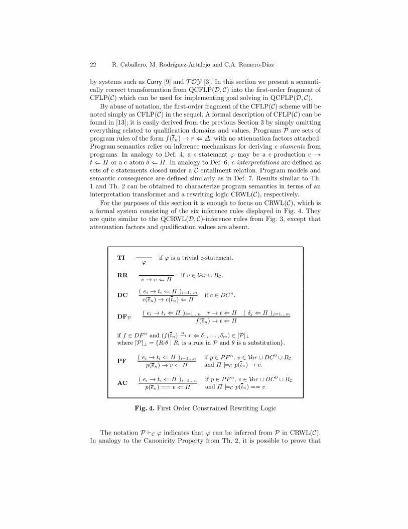
For the purposes of this section it is enough to focus on CRWL(C), which isa formal system consisting of the six inference rules displayed in Fig. 4. Theyare quite similar to the QCRWL(D, C)-inference rules from Fig. 3, except thatattenuation factors and qualification values are absent.
TIϕ
if ϕ is a trivial c-statement.
RRv → v ⇐ Π
if v ∈ Var ∪BC.
DC( ei → ti ⇐ Π )i=1...n
c(en) → c(tn) ⇐ Πif c ∈ DCn.
DFP
( ei → ti ⇐ Π )i=1...n r → t⇐ Π ( δj ⇐ Π )j=1...m
f(en) → t⇐ Π
if f ∈ DFn and (f(tn)α−→ r ⇐ δ1, . . . , δm) ∈ [P ]⊥
where [P ]⊥ = Rlθ | Rl is a rule in P and θ is a substitution.
PF( ei → ti ⇐ Π )i=1...n
p(en) → v ⇐ Π
if p ∈ PFn, v ∈ Var ∪DC0 ∪BC
and Π |=C p(tn) → v.
AC( ei → ti ⇐ Π )i=1...n
p(en) == v ⇐ Π
if p ∈ PFn, v ∈ Var ∪DC0 ∪BC
and Π |=C p(tn) == v.
Fig. 4. First Order Constrained Rewriting Logic
The notation P ⊢C ϕ indicates that ϕ can be inferred from P in CRWL(C).In analogy to the Canonicity Property from Th. 2, it is possible to prove that
A Generic Scheme for QCFLP 23
the least model of P w.r.t. set inclusion can be characterized as SP = ϕ |ϕ is a c-fact and P ⊢C ϕ. Therefore, working with formal inference in the rewritelogics QCRWL(D, C) and CRWL(C) is sufficient for proving the semantic cor-rectness of the transformations presented in the rest of this section.
The following definition is similar to Def. 9. It will be useful for proving thecorrectness of the goal solving procedure for QCFLP(D, C)-goals discussed inthe final part of this section.
Definition 10 (CFLP(C)-Goals and their Solutions). Assume a CFLP(C)-program P. Then:
1. A goal G for P has the form δ1, . . . , δm where δj are atomic C-constraints.2. A solution for G is any pair 〈σ,Π〉 such that σ is a substitution, Π is a
finite set of atomic primitive C-constraints, and P ⊢C δjσ ⇐ Π holds for1 ≤ j ≤ m. The set of all solutions for G is noted SolP(G). ⊓⊔
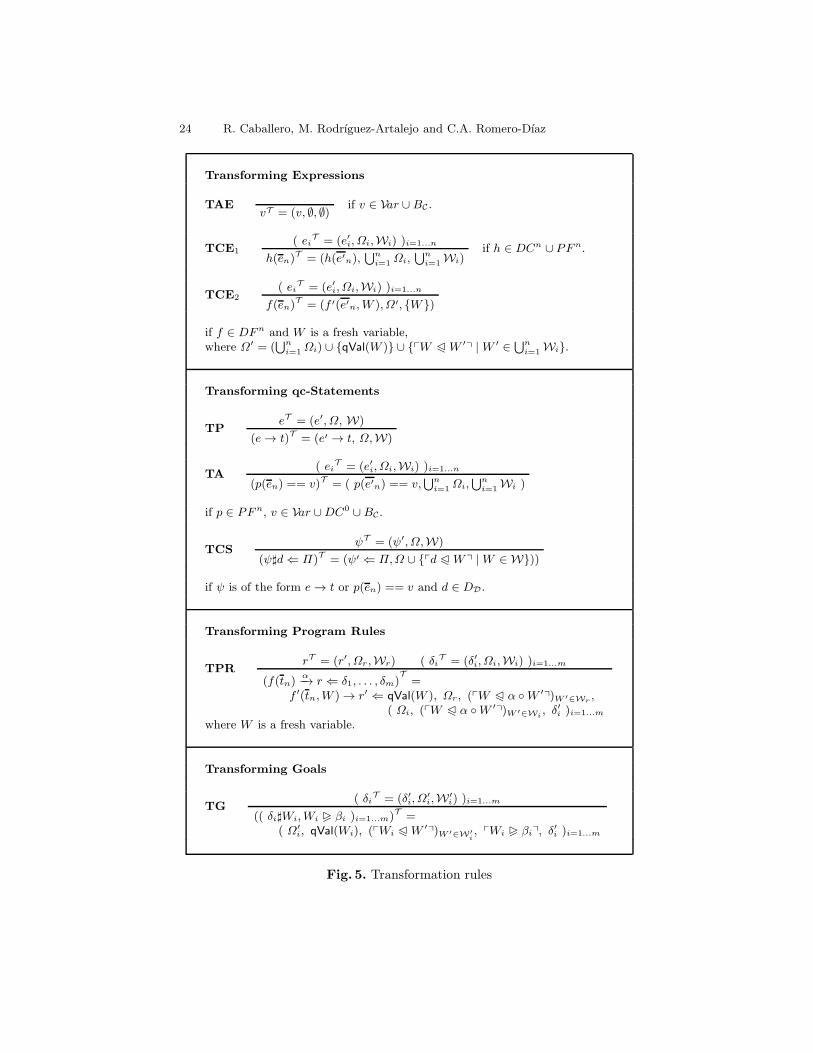
Now we are ready to describe a semantically correct transformation fromQCFLP(D, C) into CFLP(C). The transformation goes from a source signatureΣ into a target signature Σ′ such that each f ∈ DFn in Σ becomes f ′ ∈DFn+1 in Σ′, and all the other symbols in Σ remain the same in Σ′. Thereare four group of transformation rules displayed in Figure 5 and designed totransform expressions, qc-statements, program rules and goals, respectively. Thetransformation works by introducing fresh qualification variablesW to representthe qualification values attached to the results of calls to defined functions, aswell as qualification constraints to be imposed on the values of qualificationvariables. Let us comment the four groups of rules in order.
Transforming any expression e yields a triple eT = (e′, Ω,W), whereΩ is a setof qualification constraints and W is the set of qualification variables occurringin e′ at outermost positions. This set is relevant because the qualification valueattached to e cannot exceed the infimum in D of the values of the variablesW ∈W , and eT is computed by recursion on e’s syntactic structure as specified bythe transformation rules TAE, TCE1 and TCE2. Note that TCE2 introducesa new qualification variable W for each call to a defined function f ∈ DFn andbuilds a set Ω′ of qualification constraints ensuring that W must be interpretedas a qualification value not greater than the qualification values attached to f ’sarguments. TCE1 deals with calls to constructors and primitive functions justby collecting information from the arguments, and TAE is self-explanatory.
Unconditional productions and atomic constraints are transformed by meansof TP and TA, respectively, relying on the transformation of expressions in theobvious way. Relying on TP and TA, TCS transforms any qc-statement of theform ψ♯d ⇐ Π into a c-statement whose conditional part includes, in additionto Π , the qualification constraints Ω coming from ψT and extra qualificationconstraints ensuring that d is not greater than allowed by ψ’s qualification.
Program rules are transformed by TPR. Transforming the left-hand sidef(tn) introduces a fresh symbol f ′ ∈ DFn+1 and a fresh qualification variableW . The transformed right-hand side r′ comes from rT , and the transformedconditions are obtained from the constraints coming from rT and δi
T (1 ≤ i ≤ m)
24 R. Caballero, M. Rodrıguez-Artalejo and C.A. Romero-Dıaz
Transforming Expressions
TAEvT = (v, ∅, ∅)
if v ∈ Var ∪ BC.
TCE1
( eiT = (e′i, Ωi,Wi) )i=1...n
h(en)T = (h(e′n),
⋃n
i=1Ωi,
⋃n
i=1Wi)
if h ∈ DCn ∪ PFn.
TCE2
( eiT = (e′i, Ωi,Wi) )i=1...n
f(en)T = (f ′(e′n,W ),Ω′, W )
if f ∈ DFn and W is a fresh variable,where Ω′ = (
⋃n
i=1Ωi) ∪ qVal(W ) ∪ pW P W ′q |W ′ ∈
⋃n
i=1Wi.
Transforming qc-Statements
TPeT = (e′, Ω, W)
(e→ t)T = (e′ → t, Ω,W)
TA( ei
T = (e′i, Ωi,Wi) )i=1...n
(p(en) == v)T = ( p(e′n) == v,⋃n
i=1Ωi,
⋃n
i=1Wi )
if p ∈ PFn, v ∈ Var ∪DC0 ∪ BC.
TCSψT = (ψ′, Ω,W)
(ψ♯d⇐ Π)T = (ψ′ ⇐ Π,Ω ∪ pd P W q |W ∈ W))
if ψ is of the form e→ t or p(en) == v and d ∈ DD.
Transforming Program Rules
TPRrT = (r′, Ωr,Wr) ( δi
T = (δ′i, Ωi,Wi) )i=1...m
(f(tn)α−→ r ⇐ δ1, . . . , δm)
T
=f ′(tn,W ) → r′ ⇐ qVal(W ), Ωr, (pW P α W ′q)W ′∈Wr
,
( Ωi, (pW P α W ′q)W ′∈Wi, δ′i )i=1...m
where W is a fresh variable.
Transforming Goals
TG( δi
T = (δ′i, Ω′i,W
′i) )i=1...m
(( δi♯Wi,Wi Q βi )i=1...m)T =( Ω′
i, qVal(Wi), (pWi P W ′q)W ′∈W′i, pWi Q βiq, δ
′i )i=1...m
Fig. 5. Transformation rules

A Generic Scheme for QCFLP 25
by adding extra qualification constraints to be imposed on W , namely qVal(W )and (pW P α W ′q)W ′∈W′ , for W ′ = Wr and W ′ = Wi (1 ≤ i ≤ m). Byconvention, (pW P α W ′q)W ′∈W′ is understood as pW P αq in case thatW ′ = ∅. The idea is that W ’s value cannot exceed the infimum in D of allthe values α β, for the different β coming from the qualifications of r and δi(1 ≤ i ≤ m).
Finally, TG transforms a goal ( δi♯Wi, Wi Q βi )i=1...m by transforming eachatomic constraint δi and adding qVal(Wi), (pWi P W ′q)W ′∈W′
iand pWi Q βiq
(1 ≤ i ≤ m) to ensure that each Wi is interpreted as a qualification valuenot bigger than the qualification computed for δi and satisfying the thresholdcondition Wi Q βi. In case that W ′
i = ∅, (pWi P W ′q)W ′∈W′iis understood as
pWi P tq.The result of applying TPR to all the program rules of a program P will
be noted as PT . The following theorem proves that QCRWL(D, C)-derivabilityfrom P corresponds to CRWL(C)-derivability from PT . Since program semanticsin QCFLP(D, C) and in CFLP(C) is characterized by, respectively, derivabilityin QCRWL(D, C) and in CRWL(C), the program transformation is semanticallycorrect. The theorem uses an auxiliary lemma we are proving first which indicatesthat the constraints obtained when transforming a qc-statement always admit asolution.
Lemma 5. Let ϕ = ψ♯d⇐ Π be a qc-statement such that ϕT = (ψ′ ⇐ Π,Ω′).Then exists ρ : var(Ω′)→ DD \ b solution of Ω′.
Proof. ϕT is obtained by the transformation rule TCS of Figure 5. This ruleneeds to obtain ψT which can be done using either the transformation rule TPor TA of the same figure. In the case of using TP, ψ must be of the form(e → t) and Ω′ will be of the form Ω ∪ pd P Wq | W ∈ W, with Ω,Wsuch that eT = (e′, Ω,W). Checking the transformation rules for expressions(again Figure 5) we see that Ω is a set of constraints where each element iseither of the form pW P W ′q or qVal(W ), with W,W ′ ∈ War. Then ρ can bedefined assigning t to every variable W occurring in either Ω′ or W . The casecorresponding to the transformation rule TA is analogous. ⊓⊔
Theorem 3. Let P be a QCFLP(D, C)-program and ψ♯d ⇐ Π a qc-statement
such that (ψ♯d⇐ Π)T = (ψ′ ⇐ Π,Ω′). Then the two following statements areequivalent:
1. P ⊢D,C ψ♯d⇐ Π.2. PT ⊢C ψ′ρ⇐ Π for some ρ ∈ SolC(Ω
′) such that vdom(ρ) = var(Ω′).
Proof. We prove the equivalence separately proving each implication.
[1. ⇒ 2.] (Transformation completeness). Assume P ⊢D,C ψ♯d ⇐ Π by meansof a QCRWL(D, C) proof tree T with k nodes. By induction on k we show theexistence of a CRWL(C) proof tree T ′ witnessing PT ⊢C ψ′ρ ⇐ Π for someρ ∈ SolC(Ω
′) such that vdom(ρ) = var(Ω′).
Basis (k=1). If T contains only one node the QCRWL(D, C) inference step ap-plied at the root must be one of the following:
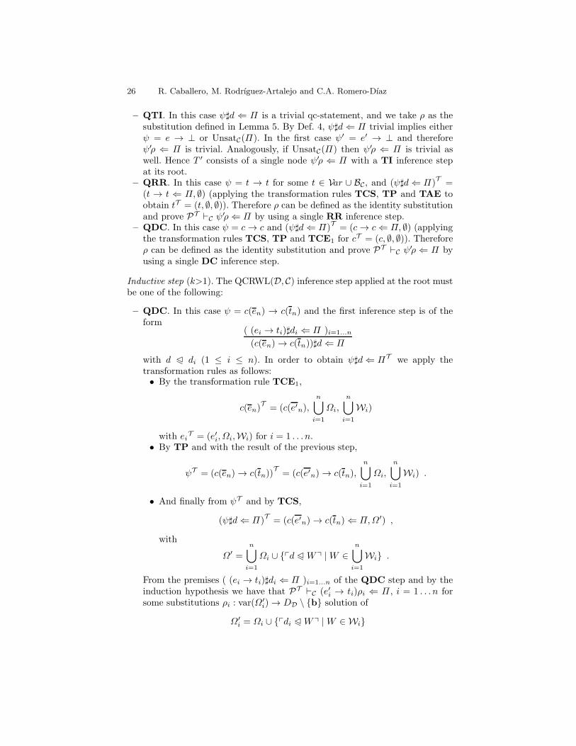
26 R. Caballero, M. Rodrıguez-Artalejo and C.A. Romero-Dıaz
– QTI. In this case ψ♯d ⇐ Π is a trivial qc-statement, and we take ρ as thesubstitution defined in Lemma 5. By Def. 4, ψ♯d⇐ Π trivial implies eitherψ = e → ⊥ or UnsatC(Π). In the first case ψ′ = e′ → ⊥ and thereforeψ′ρ ⇐ Π is trivial. Analogously, if UnsatC(Π) then ψ′ρ ⇐ Π is trivial aswell. Hence T ′ consists of a single node ψ′ρ ⇐ Π with a TI inference stepat its root.
– QRR. In this case ψ = t → t for some t ∈ Var ∪ BC, and (ψ♯d⇐ Π)T
=(t → t ⇐ Π, ∅) (applying the transformation rules TCS, TP and TAE toobtain tT = (t, ∅, ∅)). Therefore ρ can be defined as the identity substitutionand prove PT ⊢C ψ′ρ⇐ Π by using a single RR inference step.
– QDC. In this case ψ = c→ c and (ψ♯d⇐ Π)T= (c→ c⇐ Π, ∅) (applying
the transformation rules TCS, TP and TCE1 for cT = (c, ∅, ∅)). Thereforeρ can be defined as the identity substitution and prove PT ⊢C ψ′ρ ⇐ Π byusing a single DC inference step.
Inductive step (k>1). The QCRWL(D, C) inference step applied at the root mustbe one of the following:
– QDC. In this case ψ = c(en) → c(tn) and the first inference step is of theform
( (ei → ti)♯di ⇐ Π )i=1...n
(c(en)→ c(tn))♯d⇐ Π
with d P di (1 ≤ i ≤ n). In order to obtain ψ♯d⇐ ΠT we apply thetransformation rules as follows:• By the transformation rule TCE1,
c(en)T= (c(e′n),
n⋃
i=1
Ωi,
n⋃
i=1
Wi)
with eiT = (e′i, Ωi,Wi) for i = 1 . . . n.
• By TP and with the result of the previous step,
ψT = (c(en)→ c(tn))T= (c(e′n)→ c(tn),
n⋃
i=1
Ωi,
n⋃
i=1
Wi) .
• And finally from ψT and by TCS,
(ψ♯d⇐ Π)T = (c(e′n)→ c(tn)⇐ Π,Ω′) ,
with
Ω′ =
n⋃
i=1
Ωi ∪ pd P Wq |W ∈n⋃
i=1
Wi .
From the premises ( (ei → ti)♯di ⇐ Π )i=1...n of the QDC step and by theinduction hypothesis we have that PT ⊢C (e′i → ti)ρi ⇐ Π , i = 1 . . . n forsome substitutions ρi : var(Ω
′i)→ DD \ b solution of
Ω′i = Ωi ∪ pdi P Wq |W ∈ Wi

A Generic Scheme for QCFLP 27
for i = 1 . . . n. Since var(Ω′i) ∩ var(Ω′
j) = ∅ for every 1 ≤ i, j ≤ n, i 6= j,
and var(Ω′) =⋃n
i=1var(Ω′
i), we can define a new substitution ρ : var(Ω′)→DD \ b as ρ =
⊎n
i=1ρi. It is easy to check that ρ is solution of Ω′:
• It is solution of every Ω′i for i = 1 . . . n, since ρvar(Ω′
i) = ρi. Thereforeit is solution of
⋃n
i=1Ωi.
• It is a solution of pd P Wq | W ∈⋃n
i=1Wi because as solution of
Ω′i for i = 1 . . . n, ρ is solution of pdi P Wq | W ∈ Wi, and by the
hypothesis of QDC d P di.
Therefore we prove PT ⊢C (c(e′n)ρ → c(tn))ρ ⇐ Π with a proof tree T ′
which starts with a DC inference rule of the form
(( e′i → ti)ρ⇐ Π )i=1...n
(c(e′n)→ c(tn))ρ⇐ Π.
In order to justify that PT ⊢C (e′i → ti)ρ ⇐ Π for each i = 1 . . . n, weobserve that the only variables of e′i → ti that can be affected by ρ are thoseintroduced in e′i by the transformation, and that therefore (e′i → ti)ρ =(e′i → ti)ρi for i = 1 . . . n, and these premises correspond to the inductivehypotheses of this case.
– QDFP . In this case ψ = f(en) → t and the inference step applied at theroot is of the form
( (ei → tiθ)♯di ⇐ Π )i=1...n (rθ → t)♯d′0 ⇐ Π ( δjθ♯d′j ⇐ Π )j=1...m
(f(en)→ t)♯d⇐ Π
for some program rule Rl = (f(tn)α−→ r ⇐ δm) ∈ P and substitution θ such
that Rlθ ∈ [P ]⊥, and with d P di (1 ≤ i ≤ n) and d P α d′j (0 ≤ j ≤ m).
The inductive hypotheses in this case are:
1. PT ⊢C (e′i → tiθ)ρi ⇐ Π for i = 1 . . . n, with eiT = (e′i, Ωi,Wi) and ρi
solution of Ω′i = Ωi ∪ pdi P W ′q |W ′ ∈ Wi, for i = 1 . . . n.
2. PT ⊢C (r′θ → t)ρ′0 ⇐ Π , with rT = (r′, Ωr,W′0) (it is easy to check that
if rT = (r′, Ωr,W ′0) then (rθ)
T= (r′θ,Ωr,W ′
0) for every substitution θ),and ρ′0 solution of Ω′
r = Ωr ∪ pd′0 P W ′q |W ′ ∈ W ′0.
3. PT ⊢C (δ′jθ)ρ′j ⇐ Π with δj
T = (δ′j , Ωδj ,W′j) for j = 1 . . . k (it is easy
to check that if δjT = (δ′j , Ωδj ,W
′j) then (δjθ)
T= (δ′jθ,Ωδj ,W
′j) for
every substitution θ and j = 1 . . . k). The substitution ρ′j is solution ofΩ′
δj= Ωδj ∪ pd
′j P W ′q |W ′ ∈ W ′
j for j = 1 . . .m.
In this case, (ψ♯d⇐ Π)T is obtained by means of the transformation ruleTCS. This rule asks first for the transformation of the qualified statement(f(en)→ t)♯d, which can be obtained by rule TP, and this one requires thetransformation of f(en), provided by rule rule TCE2. Let’s see it:

28 R. Caballero, M. Rodrıguez-Artalejo and C.A. Romero-Dıaz
( eiT = (e′i, Ωi,Wi) )i=1...n
f(en)T= ( f(e′n,W ),
(⋃n
i=1Ωi) ∪ qVal(W ) ∪
pW P W ′q |W ′ ∈⋃n
i=1Wi, W )
TCE2
(f(en)→ t)T = ( f(e′n,W )→ t,(⋃n
i=1Ωi) ∪ qVal(W ) ∪
pW P W ′q |W ′ ∈⋃n
i=1Wi, W )
TP
((f(en)→ t)♯d⇐ Π)T = ( f(e′n,W )→ t⇐ Π,(⋃n
i=1Ωi) ∪ qVal(W ) ∪
pW P W ′q |W ′ ∈⋃n
i=1Wi ∪ pd P Wq )
TCS
Therefore
Ω′ = (
n⋃
i=1
Ωi) ∪ qVal(W ) ∪ pW P W ′q |W ′ ∈n⋃
i=1
Wi ∪ pd P Wq .
We define a new substitution
ρ =
n⊎
i=1
ρi ⊎ ρ′0 ⊎
m⊎
j=1
ρ′j ⊎ W 7→ d .
It is straightforward to check that ρ is a solution for Ω′ because ρ is solutionof:• Each Ωi (1 ≤ i ≤ n), because ρi is solution of Ω′
i which contains Ωi (seeinductive hypothesis 1) and ρ is an extension of ρi.• qVal(W ) because qVal(W )ρ = qVal(d) which holds by definition.• pW P W ′q | W ′ ∈
⋃n
i=1Wi because Wρ = d, ρ is solution of pdi P
W ′q | W ′ ∈ Wi for each i = 1 . . . n (see inductive hypothesis 1), andd P di (1 ≤ i ≤ n) by the hypotheses of the inference rule QDPP .• pd P Wq since Wρ = d and trivially d P d.
The transformed of the program rule Rl = (f(tn)α−→ r⇐ δm) ∈ P will be a
program rule in PT of the form:
(Rl)T= (f(tn,W )→ r′ ⇐ qVal(W ), Ωr , (pW P α W ′q)W ′∈W′
0,
Ωδ1 , (pW P α W ′1q)W ′
1∈W′
1, δ′1
...Ωδm , (pW P α W ′
mq)W ′m∈W′
m, δ′m

A Generic Scheme for QCFLP 29
with rT = (r′, Ωr,W ′0) and ( δj
T = (δ′j , Ωδj ,W′j) )j=1...m.
Then we prove (f(e′n,W ) → t)ρ ⇐ Π in CFLP(C) with a DFP root in-
ference step using the program rule (Rl)T
and the substitution θ′ = θ ⊎ ρto instantiate the program rule. We next check that every premise of thisinference can be proven in CRWL(C):• PT ⊢C (e′iρ → ti(θ ⊎ ρ)) ⇐ Π for i = 1 . . . n. We observe that the onlyvariables of e′i that can be affected by ρ are those in ρi. Moreover, ρcannot affect ti because the program transformation does not introducenew variables in terms. Therefore (e′iρ → ti(θ ⊎ ρ)) = (e′i → tiθ)ρi andPT ⊢C (e′i → tiθ)ρi ⇐ Π for i = 1 . . . n follows from inductive hypothesisnumber 1.• PT ⊢C (Wρ→W (θ⊎ρ))⇐ Π . By construction of ρ, (Wρ→W (θ⊎ρ)) =d→ d and one RR inference step proves this statement.• PT ⊢C (r′(θ⊎ ρ)→ tρ)⇐ Π . In this case tρ = t because t it contains novariables introduced during the transformation, and r′(θ ⊎ ρ) = r′(θρ′0)since ρ′0 is the only part of ρ that can affect r′ and the range of θdoes not include any of the new variables in the domain of ρ′0. Now,PT ⊢C (r′θ → t)ρ′0 ⇐ Π follows from inductive hypothesis number 2.• PT ⊢C qVal(W )(θ ⊎ ρ)⇐ Π . W is a fresh variable and, by constructionof ρ, qVal(W )(θ ⊎ ρ) = qVal(d). PT ⊢C qVal(d)⇐ Π trivially holds.• PT ⊢C Ωr(θ ⊎ ρ) ⇐ Π . Ωr(θ ⊎ ρ) = Ωrρ = Ωrρ
′0 and, by construction,
ρ′0 is solution of Ωr.• PT ⊢C (pW P α W ′q)(θ ⊎ ρ)⇐ Π for each W ′ ∈ W ′
0. We have (pW PαW ′q)(θ⊎ρ) = (pW P αW ′q)ρ = pWρ P αW ′ρ′0q = pd P αW ′ρ′0q.And pd P α W ′ρ′0q holds because d P α d′0 by the hypotheses of theinference rule QDPP , and pd′0 P W ′q by inductive hypothesis number2.• PT ⊢C Ωδj (θ ⊎ ρ) ⇐ Π for j = 1 . . .m. As in the previous premisesΩδj (θ ⊎ ρ) = Ωδjρ = Ωδjρ
′j and ρ′j is solution of Ωδj as a consequence of
the inductive hypothesis number 3.• PT ⊢C (pW P α W ′
jq)(θ ⊎ ρ)⇐ Π for every W ′j ∈ W
′j and j = 1 . . .m.
We have (pW P αW ′jq)(θ⊎ρ) = (pW P αW ′
jq)ρ = pWρ P αW ′jρq =
pd P α W ′jρ
′jq. Now, from the hypotheses of the inference rule QDPP
follows d P α d′j for j = 1 . . .m, and from inductive hypothesis number
3, ρ′j is solution of pd′j P W ′jq. Hence P
T ⊢C pd P α W ′jρ
′jq ⇐ Π for
j = 1 . . . k.• PT ⊢C δ′j(θ⊎ρ)⇐ Π for j = 1 . . .m. In this case δ′j can contain variables
from both θ and ρ′j . Hence δ′j(θ⊎ρ) = (δ′jθ)ρ
′j . And P
T ⊢C (δ′jθ)ρ′j ⇐ Π
follows from the inductive hypothesis number 3.– QPF. In this case ψ = p(en)→ v and the inference step applied at the root
is of the form( (ei → ti)♯di ⇐ Π )i=1...n
(p(en)→ v)♯d⇐ Π
with v ∈ Var ∪DC0 ∪BC , Π |=C p(tn)→ v and d P di (1 ≤ i ≤ n). In order
to obtain (ψ♯d⇐ Π)T one has to:

30 R. Caballero, M. Rodrıguez-Artalejo and C.A. Romero-Dıaz
• First, apply the transformation rule TCE1,
p(en)T = (p(e′n),
n⋃
i=1
Ωi,n⋃
i=1
Wi)
where eiT = (e′i, Ωi,Wi) for i = 1 . . . n.
• Second, apply the transformation rule TP,
(p(en)→ v)T = (p(e′n)→ v,
n⋃
i=1
Ωi,
n⋃
i=1
Wi) .
• And finally, apply the transformation rule TCS,
(ψ♯d⇐ Π)T = (p(e′n)→ v ⇐ Π,
n⋃
i=1
Ωi ∪ pd P Wq |W ∈n⋃
i=1
Wi) .
Therefore
Ω′ =
n⋃
i=1
Ωi ∪ pd P Wq |W ∈n⋃
i=1
Wi .
From the premises ( (ei → ti)♯di ⇐ Π )i=1...n of the inference ruleQPF, andby the inductive hypothesis we have PT ⊢C (e′i → ti)ρi ⇐ Π (1 ≤ i ≤ n) forsome substitutions ρi : var(Ω
′i)→ DD \ b solution of
Ω′i = Ωi ∪ pdi P Wq |W ∈ Wi
for i = 1 . . . n. We define a new substitution ρ : var(Ω′) → DD \ b asρ =
⊎n
i=1ρi. It is easy to check that ρ is solution of Ω′:
• It is solution of every Ω′i for i = 1 . . . n, since ρvar(Ω′
i) = ρi. Thereforeit is solution of
⋃ni=1
Ωi.• It is a solution of pd P Wq | W ∈
⋃n
i=1Wi because as solution of
Ω′i for i = 1 . . . n, ρ is solution of pdi P Wq | W ∈ Wi, and by the
hypothesis of the inference rule QPF, d P di (1 ≤ i ≤ n).We now prove PT ⊢C (p(e′n) → v)ρ ⇐ Π with a proof tree T ′ with a PFroot inference of the form:
( (e′i → ti)ρ⇐ Π )i=1...n
(p(e′n)ρ→ v)⇐ Π
The rule can be applied because the requirements v ∈ Var ∪ DC0 ∪ BC
and Π |=C p(tn) → v are ensured by the hypothesis of the inference ruleQPF. In order to justify that PT ⊢C (e′i → ti)ρ ⇐ Π for each i = 1 . . . n,we observe that the only variables of (e′i → ti) that can be affected by ρare those introduced in e′i by the transformation, and that therefore (e′i →ti)ρ = (e′i → ti)ρi for i = 1 . . . n, and it is easy to check that these premisescorrespond to the inductive hypotheses of this case.
– QAC. This case is analogous to the previous proof, with the only differencesbeing:

A Generic Scheme for QCFLP 31
• The inference rule applied at the root of the proof tree is a QAC infer-ence rule instead of a QPF inference rule.• In order to obtain the (ψ♯d⇐ Π)T , the transformation rules applied areTA and TCS instead of TCE1, TP and TCS.• The proof tree T ′ will have an AC inference step at its root instead ofa PF inference step.
[2.⇒ 1.] (Transformation soundness).Assume ρ ∈ SolC(Ω′) such that vdom(ρ) =
var(Ω′) and PT ⊢C ψ′ρ⇐ Π by means of a CRWL(C) proof tree T with k nodes.Reasoning by induction on k we show the existence of a QCRWL(D, C) prooftree T ′ witnessing P ⊢D,C ψ♯d⇐ Π .
Basis (k=1). If T contains only one node the QCRWL(D, C) inference step ap-plied at the root must be any of the following:
– TI. In this case ψ′ρ ⇐ Π is a trivial c-statement. Then ψ′ρ is either ofthe form e′ → ⊥ or UnsatC(Π). In the first case, since the transformationintroduces no new variables at the right-hand side of a production, ψ′ isof the form e′′ → ⊥ with e′ = e′′ρ, and ψ is of the form e → ⊥, henceψ♯d ⇐ Π is trivial. Analogously, if UnsatC(Π) then ψ♯d ⇐ Π is trivial aswell. Therefore T ′ consists of a single node ψ♯d ⇐ Π with d any value inDD \ b, with a QTI inference step at its root.
– RR. In this case ψ′ρ = v → v with v ∈ Var ∪ BC . Then ψ′ = v1 → v2 forsome v1, v2 ∈ Var ∪BC such that ψ′ρ = v → v. Since ψ′ cannot contain newvariables introduced by the transformation (by the transformation rules),this means ψ′ρ = ψ′, and then ψ′ = v → v. Therefore ψ = v → v, and T ′
consists of a single node containing (v → v)♯d⇐ Π for any d ∈ DD \ b asthe conclusion of a QRR inference step.
– DC. Then ψ′ρ = c→ c, which means that ψ′ can be either of the form c→ c,X → c, or X → Y with X,Y variables. In every case ψ′ does not include newvariables introduced by the transformation, and therefore ψ′ρ = ψ′, whichmeans that ψ′ = c → c is the only possibility. Therefore ψ = c → c, and T ′
consists of a single node containing (c → c)♯d ⇐ Π for some d ∈ DD \ bas the conclusion of a QDC inference step.
Inductive step (k>1). The CRWL(C) inference step applied at the root must beany of the following:
– DC. Then ψ′ρ = c(e′′n) → c(tn) where c ∈ DCn and n > 0, which impliesthat ψ = c(en) → c(tn) for values ei verifying ei
T = (e′i, Ωi,Wi) for i =1 . . . n, and e′′i = e′iρ for i = 1 . . . n. Then
ψT = (c(en)→ c(tn))T= (c(e′n)→ c(tn),
n⋃
i=1
Ωi,n⋃
i=1
Wi)
and thus ϕ = (c(en) → c(tn))♯d ⇐ Π for some d ∈ DD \ b such thatϕT = (ψ′ ⇐ Π,Ω′), with
Ω′ =
n⋃
i=1
Ωi ∪ pd P Wq |W ∈n⋃
i=1
Wi

32 R. Caballero, M. Rodrıguez-Artalejo and C.A. Romero-Dıaz
The substitution ρ : var(Ω′) → DD \ b must be solution of Ω′, and theinference step at the root must be of the form:
( e′iρ→ ti ⇐ Π )i=1...n
c(e′n)ρ→ c(tn)⇐ Π
In the premises we have the proofs Ti of PT ⊢C e′iρ⇐ Π for i = 1 . . . n. Now,for each 1 ≤ i ≤ n we obtain a new value di ∈ DD \b as di =
dWρ | W ∈
Wi. Then we will prove P ⊢D,C ϕ applying the following QDC inferencestep at the root:
( (ei → ti)♯di ⇐ Π )i=1...n
(c(en)→ c(tn))♯d⇐ Π
In order to ensure that this step must be applied we must check that d Pdi (1 ≤ i ≤ n). This holds because ρ is solution of Ω′, in particular ofpd P Wq | W ∈ Wi for i = 1 . . . n. Therefore for each i = 1 . . . n andW ∈ Wi, d P Wρ, which means that d P di =
dWρ | W ∈ Wi. To
complete the proof we must check that there are proof trees for the premises,i.e. that P ⊢D,C ϕi with ϕi = (ei → ti)♯di ⇐ Π , i = 1 . . . n. This is aconsequence of the inductive hypotheses since for each i = 1 . . . n:
• ϕiT = (e′i → ti ⇐ Π,Ω′
i), with Ω′i = Ωi ∪ pdi P Wq |W ∈ Wi.
• ρ is solution of Ω′i, since it is solution of Ωi and by the definition of di,
di P Wρ for every W ∈ Wi.
• We have that PT ⊢C e′iρ ⇐ Π for i = 1 . . . n (the premises of the DCstep).
– DFP . The inference step at the root of T will use an instance (RlT )θ ∈ [PT ]⊥
of a program rule RlT of PT . Rl
T will be the transformed of a program ruleRl = (f(tn)
α−→ r ⇐ δm) ∈ P , and therefore will have the form:
RlT = (f(tn,W )→ r′ ⇐ qVal(W ), Ωr , (pW P α W ′q)W ′∈W′
0,
Ωδ1 , (pW P α W ′1q)W ′
1∈W′
1, δ′1
...Ωδm , (pW P α W ′
mq)W ′m∈W′
m, δ′m
with rT = (r′, Ωr,W ′0) and (δj
T = (δ′j , Ω′j ,W
′j))j=1...m.
In this case, ψ′ρ must be of the form (f(e′n+1) → t)ρ. By the theorem
premises, there exists a qc-statement ψ♯d ⇐ Π such that (ψ♯d⇐ Π)T
=(ψ′ ⇐ Π,Ω′) for some Ω′. Examining the transformation program rules weobserve that the only possibility for ψ is to be of the form f(en) → t andthat the TCS transformation rules should have been applied followed by TPand TCE2. This means in particular that d 6= b and that ei
T = (e′i, Ωi,Wi)for i = 1 . . . n and that e′n+1 = V with V fresh variable. Hence
ψT = (f(e′n, V )→ t, (⋃n
i=1Ωi) ∪ qVal(V )∪
pV P W ′q |W ′ ∈⋃n
i=1Wi, V )

A Generic Scheme for QCFLP 33
and ϕ = (f(en)→ t)♯d⇐ Π for some d ∈ DD \ b. By hypotheses, ρ issolution of
Ω′ = (n⋃
i=1
Ωi) ∪ qVal(V ) ∪ pV P W ′q |W ′ ∈n⋃
i=1
Wi ∪ pd P V q
which means, in particular, that Vρ ∈ DD \ b, since it must hold bothqVal(V ) and pd P V q.Therefore the root of T will be f(e′n, V )ρ → t ⇐ Π , with premises prooftrees proving:
1. PT ⊢C ( e′iρ→ tiθ ⇐ Π )i=1...n.2. PT ⊢C ( Vρ → Wθ ⇐ Π ). Since Vρ ∈ DD \ b then either Wθ = Vρ
or Wθ = b. By premise 4 below, Wθ 6= b, therefore Wθ = Vρ.3. PT ⊢C r′θ → t⇐ Π .4. PT ⊢C qVal(Wθ)⇐ Π .5. PT ⊢C Ωrθ ⇐ Π .6. PT ⊢C (pW P α W ′q)W ′∈W′
0θ ⇐ Π .
7. PT ⊢C Ωδjθ ⇐ Π for j = 1 . . .m.8. PT ⊢C (pW P α W ′
jq)W ′j∈W′
jθ ⇐ Π for j = 1 . . .m.
9. PT ⊢C δ′jθ ⇐ Π for j = 1 . . .m.
Then we can prove P ⊢D,C ϕ by applying a QDFP inference step of theform:
( (ei → tiθ)♯di ⇐ Π )i=1...n (rθ → t)♯d′0 ⇐ Π ( δjθ♯d′j ⇐ Π )j=1...m
(f(en)→ t)♯d⇐ Π
where
• di =dWρ |W ∈ Wi for i = 1 . . . n.
• d′0 =dWθ | W ∈ W ′
0.• d′j =
dWθ |W ∈ W ′
j for j = 1 . . .m.
For proving P ⊢D,C ϕ we need to check that
• d P di (1 ≤ i ≤ n). Since ρ is solution of Ω′, d P Wρ, and Wρ P W ′ρfor every W ′ ∈ Wi and every 1 ≤ i ≤ n. Therefore d P d
ρ(W ) | W ∈Wi = di for i = 1 . . . n.• d P α d′0. Since ρ is solution of Ω′, d P Vρ = Wθ. From premise 6,Wθ P α W ′θ for every W ′ ∈ W ′
0. Therefore d P dWθ | W ∈ W ′
0 =d′0.• d P α d′j (1 ≤ j ≤ m). Analogous to the previous point but usingpremise 8.
Finally, in order to justify the premises of the QDFP we must prove:
• P ⊢D,C (ei → tiθ)♯di ⇐ Π , which is a consequence of applying the in-ductive hypotheses to the premises 1, ( e′iρ→ tiθ ⇐ Π )i=1...n, followingthe same reasoning we applied for the premises of the DC inference.• P ⊢D,C (rθ → t)♯d′0 ⇐ Π . Analogously, is a consequence of the inductivehypothesis and of premise 3.

34 R. Caballero, M. Rodrıguez-Artalejo and C.A. Romero-Dıaz
• P ⊢D,C ( δjθ♯d′j ⇐ Π )j=1...m. Again a consequence of the inductive
hypothesis, this time applied to the premise 9.
– PF. Analogous to the proof for the DC inference step.– AC. analogous to the proof for the DC inference step. ⊓⊔
Using Theorem 3 we can prove that the transformation of goals specified inFig. 5 preserves solutions in the sense of the following result.
Theorem 4. Let G be a goal for a given QCFLP(D, C)-program P. Then, thetwo following statements are equivalent:
1. 〈σ, µ,Π〉 ∈ SolP(G).2. 〈σ ⊎ µ ⊎ ρ,Π〉 ∈ SolPT (GT ) for some ρ ∈ ValD such that vdom(ρ) is the set
of new variables W introduced by the transformation of G.
Proof. Let G = ( δi♯Wi,Wi Q βi )i=1...m, σ and µ be given. For i = 1 . . .m,consider δi
T = (δ′i, Ωi,Wi) and Ω′i = Ωi ∪ pWi P Wq |W ∈ Wi. According to
Fig. 5, GT = (Ω′i, qVal(Wi), pWi Q βiq, δ
′i)i=1...m. Then, because of Def. 9(2)
and the analogous notion of solution for CFLP(C) goals explained in Sect. 3, thetwo statements of the theorem can be reformulated as follows:
(a) Wiµ Q βi and P ⊢D,C δiσ♯Wiµ⇐ Π hold for i = 1 . . .m.(b) There exists ρ ∈ ValD with vdom(ρ) =
⋃mi=1
var(Ωi) such that ρ ∈ SolC(Ω′iµ),
Wiµ Q βi and PT ⊢C (δ′iσ)ρ⇐ Π hold for i = 1 . . .m.
[(a) ⇒ (b)] Assume (a). Note that δiσ♯Wiµ⇐ ΠT is δ′iσ ⇐ Π,Ω′iµ. Applying
Theorem 3 (with ψ = δiσ, d = Wiµ and Π) we obtain PT ⊢C (δ′iσ)ρi ⇐ Π forsome ρi ∈ SolC(Ω
′iµ) with vdom(ρi) = var(Ω′
iµ) = var(Ωi). Then (b) holds forρ =
⊎m
i=1ρi.
[(b) ⇒ (a)] Assume (b). Let ρi = ρvar(Ωi), i = 1 . . .m. Note that (b) ensuresPT ⊢C (δ′iσ)ρi ⇐ Π and ρ ∈ SolC(Ω
′iµ). Then Theorem 3 can be applied (again
with ψ = δiσ, d = Wiµ and Π) to obtain P ⊢D,C δiσ♯Wiµ⇐ Π . Therefore, (a)holds. ⊓⊔
As an example of goal solving via the transformation, we consider again thelibrary program P and the goal G discussed in the Introduction. Both belongto the instance QCFLP(U ,R) of our scheme. Their translation into CFLP(R)can be executed in the T OY system [3] after loading the Real Domain Con-straints library (cflpr). The source and translated code are publicly availableat gpd.sip.ucm.es/cromdia/qlp. Solving the transformed goal in T OY com-putes the answer announced in the Introduction as follows:
Toy(R)> qVal([W]), W>=0.65, search("German","Essay",intermediate,W) == R
R -> 4
W=<0.7, W>=0.65
sol.1, more solutions (y/n/d/a) [y]? no
The best qualification value for W provided by the answer constraints is 0.7.

A Generic Scheme for QCFLP 35
5 Conclusions
The work in this report is based on the scheme CFLP(C) for functional logicprogramming with constraints presented in [13]. Our main results are: a new pro-gramming scheme QCFLP(D, C) extending the first-order fragment of CFLP(C)with qualified computation capabilities; a rewriting logic QCRWL(D, C) charac-terizing QCFLP(D, C)-program semantics; and a transformation of QCFLP(D, C)into CFLP(C) preserving program semantics and goal solutions, that can be usedas a correct implementation technique. Existing CFLP(C) systems such as T OY[3] and Curry [9] that use definitional trees as an efficient implementation toolcan easily adopt the implementation, since the structure of definitional trees isquite obviously preserved by the transformation.
As argued in the Introduction, our scheme is more expressive than the mainrelated approaches we are aware of. By means of an example dealing with asimplified library, we have shown that instances of QCFLP(D, C) can serve as adeclarative language for flexible information retrieval problems, where qualified(rather than exact) answers to user’s queries can be helpful.
As future work we plan to extend QCFLP(D, C) and the program transfor-mation in order to provide explicit support for similarity-based reasoning, aswell as the higher-order programming features available in CFLP(C). We alsoplan to automate the program transformation, which should be embedded aspart of an enhanced version of the T OY system. Finally, we plan further re-search on flexible information retrieval applications, using different instances ofour scheme.
References
1. S. Antoy, R. Echahed, and M. Hanus. A needed narrowing strategy. Journal ofthe ACM, 47(4):776–822, 2000.
2. K. R. Apt. Logic programming. In J. van Leeuwen, editor, Handbook of Theoret-ical Computer Science, volume B: Formal Models and Semantics, pages 493–574.Elsevier and The MIT Press, 1990.
3. P. Arenas, A. J. Fernandez, A. Gil, F. J. Lopez-Fraguas, M. Rodrıguez-Artalejo, and F. Saenz-Perez. T OY, a multiparadigm declarative language.version 2.3.1, 2007. R. Caballero and J. Sanchez (Eds.), Available athttp://toy.sourceforge.net.
4. R. Caballero, M. Rodrıguez-Artalejo, and C. A. Romero-Dıaz. Similarity-basedreasoning in qualified logic programming. In PPDP ’08: Proceedings of the 10thinternational ACM SIGPLAN conference on Principles and Practice of DeclarativeProgramming, pages 185–194, New York, NY, USA, 2008. ACM.
5. R. del Vado-Vırseda. Declarative constraint programming with definitional trees.In B. Gramlich, editor, Proceedings of the 5th International Conference on Fron-tiers of Combining Systems (FroCoS’05), volume 3717 of LNCS, pages 184–199.Springer Verlag, 2005.
6. M. Gabbrielli, G. M. Dore, and G. Levi. Observable semantics for constraint logicprograms. Journal of Logic and Computation, 5(2):133–171, 1995.

36 R. Caballero, M. Rodrıguez-Artalejo and C.A. Romero-Dıaz
7. M. Gabbrielli and G. Levi. Modeling answer constraints in constraint logic pro-grams. In Proceedings of the 8th International Conference on Logic Programming(ICLP’91), pages 238–252. The MIT Press, 1991.
8. S. Guadarrama, S. Munoz, and C. Vaucheret. Fuzzy prolog: A new approach usingsoft constraint propagation. Fuzzy Sets and Systems, 144(1):127–150, 2004.
9. M. Hanus. Curry: an integrated functional logic lan-guage, version 0.8.2, 2006. M. Hanus (Ed.), Available athttp://www.informatik.uni-kiel.de/~curry/report.html.
10. J. Jaffar, M. Maher, K. Marriott, and P. J. Stuckey. Semantics of constraints logicprograms. Journal of Logic Programming, 37(1-3):1–46, 1998.
11. J. W. Lloyd. Foundations of Logic Programming, Second Edition. Springer, 1987.12. F. J. Lopez-Fraguas, M. Rodrıguez-Artalejo, and R. del Vado-Virseda. A lazy nar-
rowing calculus for declarative constraint programming. In Proceedings of the 6thInternational ACM SIGPLAN Conference on Principles and Practice of Declara-tive Programming (PPDP’04), pages 43–54. ACM Press, 2004.
13. F. J. Lopez-Fraguas, M. Rodrıguez-Artalejo, and R. del Vado-Vırseda. A newgeneric scheme for functional logic programming with constraints. Journal ofHigher-Order and Symbolic Computation, 20(1&2):73–122, 2007.
14. G. Moreno and V. Pascual. Formal properties of needed narrowing with similarityrelations. Electronic Notes in Theoretical Computer Science, 188:21–35, 2007.
15. S. Riezler. Quantitative constraint logic programming for weighted grammar appli-cations. In C. Retore, editor, Proceedings of the Logical Aspects of ComputationalLinguistics (LACL’96), volume 1328 of LNCS, pages 346–365. Springer Verlag,1996.
16. S. Riezler. Probabilistic Constraint Logic Programming. PhD thesis, Neuphilolo-gischen Fakultat del Universitat Tubingen, 1998.
17. M. Rodrıguez-Artalejo. Functional and constraint logic programming. In C. M.H. Comon and R. Treinen, editors, Constraints in Computational Logics, Theoryand Applications, volume 2002 of Lecture Notes in Computer Science, pages 202–270. Springer Verlag, 2001.
18. M. Rodrıguez-Artalejo and C. A. Romero-Dıaz. A generic scheme for qualifiedlogic programming. Technical Report SIC-1-08, Universidad Complutense, Depar-tamento de Sistemas Informaticos y Computacion, Madrid, Spain, 2008.
19. M. Rodrıguez-Artalejo and C. A. Romero-Dıaz. Quantitative logic programmingrevisited. In J. Garrigue and M. Hermenegildo, editors, Functional and LogicProgramming (FLOPS’08), volume 4989 of LNCS, pages 272–288. Springer Verlag,2008.
20. M. I. Sessa. Approximate reasoning by similarity-based SLD resolution. TheoreticalComputer Science, 275(1-2):389–426, 2002.
21. V. S. Subrahmanian. Uncertainty in logic programming: Some recollections. As-sociation for Logic Programming Newsletter, 20(2), 2007.
22. A. Tarski. A lattice-theoretical fixpoint theorem and its applications. PacificJournal of Mathematics, 5(2):285–309, 1955.