Radon - Europa
30
European Atlas of Natural Radiation | Chapter 5 - Radon 108
Transcript of Radon - Europa

European Atlas of Natural Radiation | Chapter 5 - Radon108

Chapter 5 - Radon | European Atlas of Natural Radiation 109
Chapter 5 Radon
Radon isotopes (222Rn, 220Rn) are noble, naturally oc-curring radioactive gases. They originate from the al-pha decay of radium isotopes (226Ra, 224Ra), which oc-cur in most materials in the environment, i.e. soil, rocks, raw and building materials. Radon is also found in ground and tap water. The two radon isotopes are chemically identical, but they have very different half-lives: 3.82 days for radon (222Rn) and 56 seconds for thoron (220Rn). Thus, they behave very differently in the environment. Both isotopes are alpha-emitters; their decay products are polonium, bismuth and lead isotopes.
The main source of radon in air (indoor or outdoor) is soil, where radon concentrations are very high and reach tens of Bq/m3. Radon release from soil into the atmosphere depends on radium (226Ra) concentration in soil, soil parameters (porosity, density, humidity) and weather conditions (e.g. air temperature and pressure, wind, precipitation). Outdoor radon concen-trations are relatively low and change daily and sea-sonally. These changes may be used to study the movement of air masses and other climatic condi-tions.
Radon gas enters buildings (homes, workplaces) through cracks, crevices and leaks that occur in foun-dations and connections between different materials in the building. This is due to temperature and pres-sure differences between indoors and outdoors. Indoor radon is the most important source of radiation expo-sure to the public, especially on ground floor. Radon and its decay products represent the main contributor to the effective dose of ionising radiation that people receive. Radon is generally considered as the second cause of increased risk of lung cancer (after smoking).
The only way to assess indoor radon concentration is to make measurements. Different methods exist, but the most common one is to use track-etched detec-tors. Such detectors may be used to perform long-term (e.g. annual) measurements in buildings. The ex-posure time is important because indoor radon levels change daily and seasonally. Moreover, radon concen-tration shows a high spatial variation on a local scale, and is strongly connected with geological structure, building characteristics and ventilation habits of occu-pants.
A European map of indoor radon concentration has been prepared and is displayed. It is derived from sur-vey data received from 35 countries participating on a voluntary basis.
Clockwise from top-left:
Three radon passive detectors on a desk.Source: Jose-Luis Gutierrez Villanueva.
Former uranium mine, Ciudad Rodrigo, Spain.Source: Tore Tollefsen.
Soil-gas sampling, RIM 2018 exercise, Cetyne, Czech Republic.Source: Tore Tollefsen.
Metamorphic-Variscan plutonite. Contact zone betwen old metamorphic and newly intruded (Variscan) plutonite. This is the main uranium-bearing zone, Ciudad Rodrigo, Spain.Source: Peter Bossew.
Block of flats built on alum shale, Røyken, Norway. Røyken is one of the communities in Norway with the highest indoor radon concentration.Source: Peter Bossew.

European Atlas of Natural Radiation | Chapter 5 - Radon110
NATURAL
rock, soiltexture,tectonics andseismic
press, gradient
meteorology- climate- weather episodes
anthropogeniccompartmentNATURAL
GEOLOGY
ANTHROPOGENIC
“CONFOUNDERS”
GEOGENIC RnPOTENTIAL
geogeniccompartment
permeability
emanationcoefficient
soil watercontent
Rn exposure
exchange characteristicexchange characteristic
Rn risk
influence by factors
causal flow
proxy (non-physical-causal relation)
mineralogy,texture
hydrology
personcultural factors
socioeconomic factors
house and room characteristics:- building material- insulation against ground- type of building- floor level
living habits
geochemistry
eU
Rn indoor
Rn outdoorambientdose rate indoor
distribution
Rn entry intobuilding
migrationin ground
attenuationin ground
dispersion inatmosphere
Rn exhalation
Rn soil
Rn groundwater
Ra conc.
U conc.
fallout
K, Th conc.
Radon
Introduction
Radon, 'From Rock to Risk' – The geogenic compartment
Radon is a radioactive noble gas that exists naturally in the form of three isotopes: 222Rn, 220Rn and 219Rn. The most stable and environmentally relevant one, 222Rn, hereafter called radon (Rn), is formed by alpha decay of 226Ra, and ultimately from 238U; it has a half-life of 3.82 days. On the other hand, 220Rn, hereafter called thoron (Tn), is a short-lived isotope with a half-life of 55.6 seconds.
Motivation
This chapter is devoted to describing the complex path of radon 'from rock to risk'. Some compartments are described in particular: they can be distinguished depending on whether they house natural or human-made or -induced phenomena, or depending on the medium (rock, soil, water, air) that dominates them. Emphasis is on the geogenic compartments.
Geogenic compartments
Radon source
The original sources of radon are uranium (238U, for 222Rn) and thorium (232Th, for 220Rn) in the ground. Due to their physical and chemical properties, the two radon isotopes are distributed in part similarly, and in part differently in the various environmental compartments. We distinguish between the geogenic and anthropogenic compartments.
The geogenic compartment comprises a number of connected and interacting 'sub-compartments'. These are the lithosphere (rocks); the pedosphere (soil) which is partly derived from rock, but soil can also have different origins (Aeolic – loess, alluvial /
colluvial – by sedimentation of material transported by rivers); the hydrosphere (ground and surface water bodies); and the atmosphere.
All spheres are connected and interact through exchange of
matter, technically speaking: material fluxes. For example, ground water is in contact with rock. Rock chemistry controls water chemistry and, reversely, substances dissolved in the water can precipitate into rock and modify its mineralogy, or if exhaled (such
Complexity in environmental sciencesAlthough it is difficult to define complexity, it is a keyword in
environmental sciences. It may be characterised by the following features:
• Complex systems consist of many interacting 'players' (e.g. factors, controls, quantities);
• Factors may depend upon each other in different ways and even be nested. The factors may be 'coupled' in a way that is itself a function of other factors, or convoluted in structures which are not well known;
• Yet the underlying physical laws may be simple (such as, in radon science, radioactive decay, diffusion, advection, convection, dissolution etc.);
• Often such systems develop complicated temporal and spatial patterns, with regular components, but also show a tendency to seemingly erratic spatial or temporal variability;
• Complex systems have a tendency to extreme behaviour in temporal evolution or spatial pattern;
• Patterns often look similar when viewed on different scales or 'magnifications'. Self-similarity is a characteristic of fractal behaviour. On the other hand, results may depend on the scale or resolution under which the system is viewed;
• Often it is difficult to establish clearly defined 'laboratory conditions'. Consequently, input quantities of analysis are often 'noisy' or 'dirty' to some degree. Sometimes factors are only fuzzily defined or definable.
• This reality often makes modelling, and in particular prediction and forecasting, difficult and technically demanding. Simple regression models often perform badly, because they can hardly capture a high-dimensional space of convoluted covariates.
• Usually only statistical modelling is possible, i.e. finding statistical rules which describe the behaviour of the system.
Ecological modelling can be understood as reducing the complexity by focusing on key processes. A model should be simple (Ockham’s razor), but fit for the purpose. Oversimplification is characterised by processes ill-captured, which leads to high uncertainty in terms of accuracy and precision. On the other hand, when too many components are present (which is conceptually similar to over-fitting in regression), too many uncertain and/or correlated (sensitive) model parameters may lead to a deteriorated prediction capability.
Figure 5-1.Network of radon-related quantities, 'From rock to risk'. This graph intends to visualise the complexity of the pathway - or rather network - which leads from radon sources (ultimately uranium in the ground) to the risk which is caused by radon, controlled by many factors and interactions. These are of many kinds, essentially natural and anthropogenic factors. They act on all levels of the network with different strength, again controlled by other factors.Source: Graph created by Peter Bossew.

Chapter 5 - Radon | European Atlas of Natural Radiation 111
as radon), migrate within the ground according to its permeability. Radon, in particular, is the direct decay product of two radium
isotopes: 226Ra (222Rn) and 224Ra (220Rn). The radon isotopes are relatively long-lived (especially 226Ra, with a half-life of 1 620 years), which is why they are not necessarily in equilibrium with their 'grandparents', 238U and 232Th. Mainly the action of ground water can lead to disequilibrium, due to different solubility of radium and uranium in water, resulting from their different chemical properties. This implies that the local radon production rate is not necessarily proportional to the uranium (thorium) concentration at the same point in the ground.
Radon (222Rn) and thoron (220Rn) (see Section 2.2)
Chemically, radon isotopes are identical, but due to their very different half-lives (Rn: 3.82 days vs. Tn: 56 seconds) their presence in the environment has different spatial and time patterns.
Concerning radiology and radon risk, geogenic thoron is mostly considered to be a practically negligible component, as infiltration into buildings is usually a 'slow' process that effectively removes thoron due to its short half-life. However, in (mostly old) buildings with unsealed interface to the ground, i.e. basement or ground floor directly exposed to exhalation, geogenic thoron can be a factor that should be considered. Otherwise, it seems that thoron is a problem if exhaled from thoron-containing building materials, typically raw clay, which can have a high radon exhalation rate. Close to exhaling surfaces (walls), exposure to thoron progenies can be a factor to consider.
Radon in soil gas (see Section 5.1)
Most radon that has been generated by radium decay in a rock or soil grain never leaves that grain. The fraction of radon actually being released into pore space, and available for further migration, is called emanation power. It depends on mineralogy and grain size. Mineralogy defines the crystal geometry, which in turn determines 'how easily' a radon atom generated within a crystal can escape. Grain size can be tectonically modified if strain leads to fracturation or the 'milling' of rock. Water content is controlled by meteorological conditions (how deep into the ground the impact of rain is effective, depends on soil type) and possibly by ground-water dynamics.
Radon movement in the pore space depends on water content (radon diffusive mobility is much lower in water than in air, and radon will decay in humid soil before reaching the surface, compared to dry soils), permeability at different scales, pressure difference and the presence of carriers, such as water or geogenic CO2 or methane. Diffusion driven by concentration difference also contributes. Permeability is usually understood, e.g. in the sense of Darcy's law, as a summary quantity which comprises geometrical properties without specifying them.
Still, one sometimes distinguishes between micro- and macro-permeability. The former is related to the porous structure of the soil, while the latter, to fissures or cracks, up to caves and karst phenomena, or also to ducts created by plant or animal activity. Therefore, permeability depends not only on the presence of space between grains, but also on whether the spaces are connected, so that percolation over longer distance is actually 'geometrically' possible. Percolation theory has many important applications in analysing the behaviour of networks of all kinds in nature or in the social sphere. The distribution of soil grains and spaces between them can be understood as a network. Apart from the availability of pathways in a network, quantified by connectivity, their length is also relevant. Tortuosity quantifies how bent or convoluted migration paths are.
As a summary, the effective path length between the point of Rn generation and a target point (e.g. soil surface or the interface with a building) which radon together with its carrier fluids have to travel, not only depends on the straight distance between the two points, but on the geometrical properties of the medium in which migration takes place.
Radon exhalation and radon outdoor (see Sections 5.2 - 5.3)
Once exhaled from the soil or rock surface, radon spreads in the atmosphere by diffusion, convection and advection carried by air movement. This phenomenon is being extensively studied because radon and its progeny generated in the atmosphere can serve as tracers of atmospheric processes.
In the context of this section, this behaviour is relevant only as far as outdoor radon contributes to dose and is a minor source of indoor radon.
Radon in ground water (see Chapter 6)
Radon is soluble in water. The air/water distribution coefficient depends mainly on temperature. Ground water is important, being an efficient carrier of radon and possibly a significant secondary source of indoor radon. It can be taken up by water through dissolution from its point of generation, or after some migration with other carriers, transported over quite large distances and released if the solubility conditions change. Other, but minor sources of radon in water are radium dissolved in the water and uptake from the atmosphere. Because uranium and radium have different chemical properties, no equilibrium exists between them in water (Skeppström & Olofsson, 2007).
In terms of radiological relevance, radon in drilled well water can be an important source of exposure. Pathways are ingestion and inhalation of dissolved radon.
Radon in ground-water serves as an important tracer of hydrological processes, e.g. in karst studies and speleology.
SynthesisIn a 'taxonomy' of compartments, we may distinguish between:
The geogenic compartment, which consists of:• The geosphere, in which reside:
• original sources of Rn and Tn; 238U and 232Th decay series;
• geochemical fractionation, secondary mineralisation;
• emanation from Ra bearing mineral;
• transport in the geosphere: diffusion, advection.
• The hydrosphere, which characterises:
• Rn solution / dissolution;
• Rn transport with ground water;
• Rn transport in the porous ground via influence on emanation factor and permeability.
• The outdoor atmosphere:
• dispersion and transport of Rn.
The anthropogenic compartment, which is addressed only marginally in this chapter, may be divided into:• The 'domosphere' (house ecosystem), treating:
• building construction type;
• building materials: exhalation;
• physics of the indoor atmosphere;
• attachment of Rn progenies to aerosols, adhesion to surfaces;
• influence of house usage.
• 'Type of work':
• speed and amount of air pumped by the lungs.
• The 'pneosphere' (the human respiratory system), including:
• physiology;
• radiation biology.
Interface to buildings (see Sections 5.2 and 5.4)
Radon may enter from the ground into a building. This process is controlled by driving forces and by the nature of the interface between the soil and the building. Physical mechanisms for migration are diffusion, convection and advection. The driving forces are the concentration gradient for diffusion and the pressure difference for convection and advection. In the presence of a barrier, such as a concrete slab as foundation or insulating layers, advection through small fissures is usually the dominant mechanism. The pressure gradient is generated by temperature and pressure differences indoors – outdoors.
Soil-gas sampling drill, RIM 2018 exercise, Cetyne, Czech Republic.Source: Tore Tollefsen.

European Atlas of Natural Radiation | Chapter 5 - Radon112
Radon
5.1 Radon in soil gas
5.1.1 IntroductionRadon atoms, generated in the soil or rock within the solid
mineral grains, can escape into the air or water-filled pores and further migrate by diffusion, convection and/or advection towards the surface.
In most cases, radon in soil gas is considered to be the main source of enhanced indoor radon concentrations compared to two other sources: water and building materials. (Only where the contribution from geogenic radon is small can building materials be the dominant contributor.) Research on radon behaviour and release from soils or parent rocks might have the advantage of identifying areas where indoor radon levels are expected to be high or enhanced over the existing limits. Hence, appropriate remedial actions can be taken for existing houses, or soil-gas radon can be prevented from entering newly-built houses. In addition, soil-gas radon has been found to be used in a wide range of geoscientific applications, such as tectonics, in studies of earthquakes, volcanic fluids, and surface ground water.
Several factors control radon concentration in the soil, both on daily and seasonal scales. Precipitation and temperature appear to control mainly soil-gas radon levels on a seasonal scale, whereas other climatic factors, such as barometric pressure, temperature, soil moisture and wind, affect radon concentration and behaviour on a daily scale. In order to use soil-gas sampling results to predict long-term radon concentration (e.g. over different seasons), it is necessary to know the interaction between these climatic variables and perform robust statistical analyses. Furthermore, as soil gas surveys generally cover large areas with different rock and soil characteristics, it is necessary to have a deep knowledge of the geological and soil processes affecting radon generation and transport.
Factors influencing radon concentration in soils
Geological factors
a. Uranium concentration in rocks and soils
Radon (222Rn) is a member of the uranium (238U) decay chain. 238U is present in all genetic rock types (sedimentary, metamorphic and magmatic) in varying concentrations. Generally, it can be stated that this sequence of genetic rock types also describes average uranium concentrations from the lowest (sedimentary) to the highest (magmatic). However, anomalous uranium concentrations can be found in all rock types in the form of impregnations in sedimentary deposits or vein-type deposits in metamorphic or magmatic rocks. The current methods to determine uranium concentrations are usually based on gamma-spectrometric measurements in the form of airborne measurements for large-area coverage, field or laboratory gamma spectrometry on solid samples (soils, rocks) or liquid (water) samples for detailed studies or calibration of airborne measurements. After periods of extensive uranium exploration and environmental mapping, these data are usually available in many countries and can contribute to efficient radon risk mapping (Matolín, 2017; Smethurst et al., 2017; Szabó et al., 2017; Cinelli et al., 2017; Ielsch et al., 2017). The use of radiometric data has some limitations which may be summarised as follows:1. differences between airborne and ground gamma
spectrometric data;
2. differences in regional and detailed geological mapping; and
3. the presence of factors influencing the radon migration and diffusion from deeper soil horizons to the surface and subsequently to dwellings.
b. Permeability
Soil permeability characterises the ability of the geological environment to transport radon and other soil gases from the source (parent solid or weathered rock) to the target surface or dwelling (Nazaroff & Nero, 1988; Nazaroff, 1992). Mineral grains, containing U, produce radon in a quantity characterised by the emanation coefficient. The radon escapes from the mineral grains into a pore space through diffusion, at distances of millimetres or a few centimetres. From the vicinity of a mineral grain, radon is transported into the surrounding pore spaces, and its mobility is controlled by space connections between pores and physical conditions such as temperature, pressure gradients or soil moisture. This process is called convection and propagates to distances of metres or tens or
hundreds of metres. The diffusion can be both vertically and laterally oriented. The vertical convection can be limited by the presence of sub-horizontally oriented mineral particles (like micas) or layered clay intercalations in soils or clayey weathered rocks. On the other hand, these vertical barriers close to the surface layers can trigger lateral transport under the impermeable barrier into the basement of houses, especially when the process is supported by pressure or thermal gradient. As the permeability for gases varies vertically and horizontally even in a small area of a building site, it is necessary to characterise this parameter for several points of the studied area, namely in the ground plan of the future house and its close vicinity. At present, permeability is usually determined through:1. in situ measurements by permeameters;
2. soil texture analysis; and
3. data from soil permeability maps (generally available at regional level, so cannot be used for local estimation).
c. Geological inhomogeneities
Different types of geological and man-made inhomogeneities can influence soil-gas radon concentrations at a specific local site of interest. These inhomogeneities are usually more permeable, subvertically oriented and they intersect more rock types with different radon potential. The geological inhomogeneities are mostly represented by faults of different types. The soil-gas radon convectivity of faults could depend on the position of the faults in geodynamically active or passive regions (Pereira et al., 2010; Ciotoli et al., 2007, 2016). Specifically, the proximity to the fault plane and the bedrock lithology are the main factors controlling the soil-gas radon migration velocity and concentration in the shallow soil.
According to the literature, radon anomalies above a fault vary in intensity (in particular when there is a thick sediment layer over the rock with several aquifers and no radon anomalies) and shape, and radon peak values can assume different spatial positions within the fault zone; therefore the spatial distribution of soil-radon concentration is affected by the fault geometry and activity, as well as by the volume of fractured rock involved (Ciotoli et al., 2016; Seminsky et al., 2014; Pereira et al., 2010; Koike et al., 2009; Annuziatellis et al., 2008; King et al., 1996).
In fact, the distribution of radon anomalies in faulted areas is strictly linked to the evolution of the fault zone that at first stage is generally characterised by stepwise developments of different densities of fault segments, and fractures within the fault zones across and along their strike (Fossen, 2010). Usually the faults have a thin core (Childs et al., 2009), which serves as a convective pathway for radon flux upwards. The damage zone surrounding the fault core has a wider extent for radon release, namely when the fault core is impermeable (Ciotoli et al., 2015, 2016; Seminsky et al., 2014; Pereira et al., 2010; Koike et al., 2009; Annunziatellis et al., 2008; King et al., 1996). Especially in the geodynamically active regions, the faults can express the unexpected radon variations, which depend mainly on changes in tectonic stress and strain (Ciotoli et al., 2007, 2014).
In karstic areas (Kropat et al., 2017), the radon flow strongly depends on the convective characteristics of open spaces (such as cave systems, chimneys) in karstic bedrock.
The presence of rock types with different levels of natural radioactivity changes the average radon concentrations in areas with low radon risk. Silurian black shales in low-radon limestones, black shales in metasedimentary sequences of Neoproterozoic (Barnet & Pacherová, 2013) or alum shales in Scandinavia (Sundal et al., 2004) serve as typical examples. For instance, the underlying rocks characterised by high soil-gas radon concentrations (e.g. magmatic rocks) can influence the radon level in surface layers in geodynamically stable areas of Quaternary fluvial sediments of the Czech Republic (Barnet & Pacherová, 2011), or glaciofluvial
sediments like Scandinavian eskers (Watson et al., 2017). The man-made inhomogeneities can be widely found in areas
influenced by old mining activities, where the soil-gas geodynamic regime of underground spaces can be copied to surface layer through the pits, abandoned adits (even if backfilled with inert material) or through fissures in case of subsidence areas.
Differences in natural soil-gas radon concentrations can also be found between arable soils (mostly lower radon concentrations than in the parent rock due to atmospheric release) and their intact rock equivalents.
Due to the convection of soil-gas radon, increased concentrations may also appear on the rims of artificial flat barriers such as asphalt and concrete covers, where radon accumulated under the barrier can be released in the form of anomaly levels not corresponding to the surrounding bedrock. During building activities for levelling building grounds, huge amounts of soil and rock material are often transported, and this process can change the natural radon concentration of building sites.
Variations in radiation concentration with depthRadon concentrations increase with depth (Clavensjö &
Åkerblom, 1994). At the surface layer, when disturbed by disintegrated soil particles, roots of vegetation or the presence of the soil rock structure, the radon concentration is diluted in contact with atmospheric air. The trend of increasing radon concentration with depth is not generally defined for all rock types, since local differences at soil layers and bedrock lithological types influence the radon variations with depth at a sampling site (Neznal et al., 1994, 1996). Radon concentrations measured in soils usually range between 5 and 100 kBq/m3 (with extremes up to some 10 000s) for different rock types, while concentrations in the atmosphere directly above the soil surface only reach levels of tens of Bq/m3 (with extremes up to hundreds). Therefore, representative soil-gas samples must be taken from deeper soil horizons. At present, steel-hammered probes with lost tip or drilled probes with packers are used to make sure that the undersurface cavity is opened and that the soil gas is sampled directly from the predefined depth horizon. Usually, a depth of 0.8 - 1 m is recommended for correct and economically efficient radon concentration measurements (Ciotoli et al., 1998, 2007; Neznal, 2004). These sampling devices are widely used in EU countries.
Climatic variationsSeasonal variations affect the physical processes of radon
generation in the soil gas, due to the combined effect of geological and meteorological parameters. From different sites, geological and soil factors (e.g. rock type, mineralogy, structure, etc.) may affect radon concentration at the level of a single geological unit. Furthermore, radon concentrations measured in summer cannot be used to predict radon levels in winter; this is the reason why soil-gas surveys are usually carried out in a short time and during stable weather conditions (Kraner et al., 1964; Taipale & Winqvist, 1985; Fukui, 1987; Schumann et al., 1992; Ciotoli et al., 2007).
In order to predict soil-gas radon values at different timescales (i.e., seasonal, daily), one should consider the climatic factors controlling soil-gas concentrations. In fact, a meteorological signal is generally characterised by short-term fluctuations (daily) superimposed on longer, seasonal changes (year). According to literature, the main factors affecting radon concentration in soil gas are essentially the following: soil moisture retention characteristics (e.g. permeability, porosity, grain size, and the number of consecutive rainy days); barometric pressure; soil temperature; hydrometeors occurrence (mainly snow and ice); and wind velocity (Washington & Rose, 1990; Schumann et al., 1989; Lindmark & Rosen, 1985; Clements & Wilkening, 1974).

Chapter 5 - Radon | European Atlas of Natural Radiation 113
Soil moisture and precipitationStudies of temporal variations of meteorological parameters
show a marked effect of soil moisture on radon concentration in the soil pore. An increase in soil moisture content reduces the soil permeability and availability of soil air, thus increasing the radon content of the soil by the double effects of partitioning and reduced diffusivity. In fact, radon has a non-negligible solubility in water, the partition coefficient of radon between water and air being approximately equal to 0.25 at standard conditions (Clever, 1979). Since radon also has less diffusive mobility in water than in air, it can accumulate in the water surrounding the grains of soil and consequently in the same air pores of the soil, reducing the radon flux toward the atmosphere (Arvela et al., 2016; Alharbil & Abbady, 2013; Voltaggio et al., 2006).
Radon variability due to soil moisture is probably related to the condition of water saturation and moisture retention characteristics of the terrain. This phenomenon can occur especially in highly permeable soil, where a rapid decrease of shallow soil permeability can be associated with increased moisture content (reduction of air in the pores, expansion/hydration of clays etc.). This inhibits advective and diffusive transport of radon escaping from the soil (i.e. capping effect), yielding an increase in the soil-gas radon concentration within the diffusion/advection zone (Pinault & Baubron, 1996; King & Minissale, 1994). In highly permeable and homogeneous soil, a good correlation between soil-gas radon concentration, permeability and soil moisture can be obtained, while in areas with medium or low permeable environment the correlation can often be very weak (Kraner et al., 1964; Kovach, 1945).
Effective rainfall (i.e. water saturation grade, which can be directly measured or inferred from the number of consecutive rainy days) makes the soil radon concentration increase just after the rainfall (Pinault & Baubron, 1996). During the rainy winter/spring, radon concentration may seasonally increase in soil gas, when radon tends to be trapped in the soil under a layer of water-saturated horizon characterised by reduced gas permeability (i.e. the capping effect), while during the sunny summer/autumn, it exhales more easily as the soil becomes drier and more permeable. For sites characterised by relatively high permeability, the water-saturated layer quickly extends below the sampling depth, thus resulting in minimum radon concentration during the rainy season (King & Minissale, 1994). For sites that had relatively low permeability, the wet layer was thinner than the sampling depth, and the capping effect caused higher radon values during the rainy season (Arvela et al., 2015; Rose et al., 1990). In addition, the presence of snow and ice on the soil causes accumulation of radon in the soil due to the capping effect (Lindmark & Rosen, 1985; Hesselbom, 1985; Jaacks, 1984; Kovach, 1945).
Barometric pressureBarometric pressure is another important parameter. Even
when not associated with precipitation, large-scale barometric pressure changes show an inverse correlation with soil-gas radon concentration. The magnitude of changes in radon values in response to barometric pressure changes is generally lower than that caused by soil moisture (i.e. precipitation) alone. Decreasing barometric pressure tends to draw soil gas out of the ground, increasing the radon concentration in the near-surface layers. This phenomenon is particularly pronounced in highly permeable soils, where near-surface radon-bearing soil gas escapes more rapidly into the atmosphere, generally causing a decrease in radon concentration at the 0.6 – 0.8 m sampling depth. Conversely, increasing barometric pressure forces atmospheric air into the soil, diluting the near-surface soil gas and driving radon deeper into the soil (Lindmark & Rosen, 1985; Kraner et al., 1964;
Kovach, 1945). Clements & Wilkening (1974) noted that pressure changes of 1 – 2 % associated with the passage of weather fronts could produce changes of 20 – 60 % in the radon flux, depending on the rate of pressure change and its duration.
Soil and air temperatureTemperature shows a contrasting effect with barometric
pressure. The effect of temperature on soil-gas radon concentrations appears to be minor compared to those of precipitation and barometric pressure. Some studies suggest that a decrease in air temperature is correlated with high concentrations of soil-gas radon, but this correlation is no longer evident from a depth of 0.6 m. Temperature gradients between soil and air could induce thermal convection that would cause soil gas to flow in a vertical direction (Jaack, 1984; Kovach, 1945).
Soil temperature variations can cause rapid increase in soil radon concentrations due to the enhanced radon convection that increases the mobility of radon in soil gas and the radon concentration ratio between gas and water (Washington & Rose, 1992; Memugi & Mamuro, 1973). Otherwise, increasing temperatures may also increase production of some gas carriers (CO2 and H2O vapour), which again may increase radon transport from depth (Pinault et al., 1996). Arvela et al. (2015) reported that high soil temperatures in summer increased calculated soil-gas radon concentration by 14 % with respect to winter values. Furthermore, temperature changes may play a significant role in radon accumulation during winter months, due to capping effects caused by the freezing of water in shallower soil layers. Beneath frozen layers, the soil is likely to be unfrozen and relatively permeable, so at that depth radon can concentrate to elevated levels. This phenomenon can have an important effect in producing elevated indoor radon levels during winter months in many areas.
In general, temperature and barometric pressure can have a synergistic action; for example a temperature increase and/or a barometric pressure decrease favour the flux of radon from soil to atmosphere, causing a transient disequilibrium between the flux from the deeper level of soils and the shallower levels, resulting in a non-stationary radon content.
WindHigh wind velocities cause local depressurisation and, therefore,
decreasing radon concentration in soil (Voltaggio, 2012), because the gas is diluted by atmospheric air and/or removed at surface. Wind effects have been observed up to a depth of 1.5 m (Kovach, 1945; Kraner et al., 1964). However, in addition to wind velocity, soil permeability, soil moisture and ground cover (i.e., snow, ice, etc.) may affect the magnitude and the depth to which wind can influence soil-gas radon levels. Strong wind turbulence and the Bernoulli effect across an irregular soil surface can draw soil gas upward from depths caused by alternating pumping between pressurisation and depressurisation of the soil, similarly to that caused by barometric pressure (Kovach, 1945; Jaacks, 1984; Hesselbom, 1985; Lindmark & Rosen, 1985).
5.1.2 Measurement methods Indirect and direct methods can be used to estimate the soil-
gas radon concentration. Indirect methods are based on measuring the radioactive
parent isotopes and, through calculation, result in a derived maximum level of radon activity concentration. Uranium and radium are analysed as parent isotopes for radon (more details in Section 2.2.1). The underlying assumption of this method is that there is a balance between uranium and radium.
eU is defined as the 238U concentration in radioactive equilibrium with 226Ra.
For example, a gamma spectrometer could be used to calculate the in situ eU concentration in soil or rock. Using this concentration, one may use the following formula to calculate the maximum concentration of radon activity forming in soil (Andersson et al., 1983; Clavensjö & Åkerblom, 1994):
RP
C = A . e . ß . (1 - p) p-1
C∞
(-log10(k) - 10)=
F ARa D0
0.75
. ρb .
.
λ p exp(-6 Sp - 6S14p)
D0 exp(-6 Sp - 6S14p)
J2
(m + λ222 . Co) . V
S
. ε .
. ε .
T273( )= √
(
[ ]( )
)
FTn ARa-224 ρb λTn
. e-λt . (1 - e-λt )
(C - C0e-λt )
S(1 - e-λt )
+
=
E222=
E0=
NRL=
δA δa12 + δa2
2 + δa32 + .. . + δan
2
2(Measured Mean - Reference Value
Reference Value
=
D
WL = EEC (Bq /m3)/3 700 = F *CRn (Bq /m3)/3 700
PAEE(WLM) = PAEC(WL) *
DC * EEC * t DC * F * t * CRn=
% PME × 100 +=
=
λ 220 . V0
-λ . (V / Q)220 1S
Cm
eE220
E222
=
λ . V
λ . V
1 - Φ 12 σ2x
1 - eln (Ri - R0) - µ
σ
( )Exposure (h)170
[ ]( )2
Standard Deviation
Measured Mean× 100
Ct C0=
√
√
√
-(x-µ)2
2σ2 -(x-µ)2
2σ2-∞
i 0ln (R - R )
∫
(5-1)
(5-2)
(5-4)
(5-5)
(5-7)
(5-8)
(5-9)
(5-6)
(5-10)
(5-11)
(5-12)
(5-13)
(5-14)
(5-3)√
√
NAPL Pi =−J ± −4CH
2H
π
where: C is the maximum concentration of radon capable of migrating in soil (in kBq/m³), forming at the expense of 226Ra (eU) in soil;A is the eU concentration (1 ppm U = 12.35 238U Bq/kg);e is the emanation factor (coefficient) of the lithotype;ß is the compact specific weight (relative density) (in kg/m3); andp is porosity (as a fraction).
Unfortunately, indirect methods cannot give an indication about the inflow of radon from deeper sediments or rocks, from karst cavities or from fault zones that can sometimes increase radon content by a factor of ten (Neri et al., 2016; Täht-Kok et al., 2012).
Direct methods are based on measuring the concentration of radon and its progeny decay products in a sample of soil gas (more details in Section 2.5). Since radon and its decay products emit alpha and/or beta particles as well as photons, in principle a whole range of detectors can be used for measurements in combination with a suitable sampling technique.
Direct measurement methods, whether active or passive, are recommended by the ISO11665-11:2016 international standard, 'Test method for soil gas with sampling at depth'.
In active sampling, one considers a certain soil-gas volume at a certain moment or period of time representative of the soil under investigation. The sample is transferred into the detection chamber, and activity concentration is measured with a semi-conductor or a scintillation detector. With passive methods, a detection chamber must be placed below the ground for a certain time interval, during which the transfer of the soil-gas sample into the detection chamber occurs by diffusion and the activity concentration is estimated.
Sampling
Choosing locations
Choosing the number and locations of sampling points depends on the task at hand and on the available resources, but it is highly recommended to study geological and topsoil maps of the target area first. Since samples taken from a very limited area must aim to represent a larger area than just their immediate surroundings, a sound geological knowledge is especially relevant in areas where uranium-rich rocks occur in sections of bedrock. When compiling a radon risk map for larger areas or regions, it becomes even more delicate to choose locations for sampling points, and thus a good knowledge of the existing geological context is equally essential.
Soil-gas sampling
A relatively easy way to measure radon concentration in soil gas is to use a soil-gas probe coupled with a measuring instrument. This probe can be operated anywhere above the water table and is often used in conjunction with a drying unit.
Either sucking or pumping soil gas directly into the measurement chamber or extracting soil gas from the surface using syringes are both delicate operations in the sampling procedure, because there is always a risk that environmental air may leak through the probe into the radon measuring instrument.
The entire system must be perfectly sealed. If the sampling system is not perfectly sealed or does not reach a sufficient level of underpressure to collect gas samples in soils of low permeability, the soil-gas radon concentration may be underestimated. Measurement results that indicate a radon activity concentration lower than 1 - 2 kBq/m3 are usually considered to be failures. The internal volume of the cavity, which is created at the lower end of the sampling probe, must be large enough to enable sample collection. The soil-gas samples are collected from a depth of about 1.0 m below the ground surface; for instance a depth of 0.8 m is used in the Czech Republic, Sweden, Estonia and in many other countries (Neznal, 2015), which corresponds to the ISO 11665-11:2016 international standard mentioned above, 'Test method for soil gas with sampling at depth'.
Soil-gas sampling sequence, RIM 2018 exercise, Cetyne, Czech Republic.Source: Tore Tollefsen.

European Atlas of Natural Radiation | Chapter 5 - Radon114
C∞ (kBq/m3)
-log
10 (k
(m2 )
)
010
11
12
13
14
10 20 30 40 50 60 70 80 90 100 110 120 130
HIGH RADON INDEXOF BUILDING SITERP > 35
MEDIUM RADON INDEXOF BUILDING SITE10 < RP > 35
LOW RADONINDEX OFBUILDING SITERP < 10
Radon
In soils with high permeability, such as coarse-grained gravel, sampling succeeds better during a rainy period or during winter, when the upper ground is frozen. In clay, on the contrary, better measurements are obtained during the dry season. In these cases, indirect methods can give reliable results.
In conditions of high ground-water saturation, soil gas can also be measured during a dry period. However, if peat forms the upper layer of the soil, no radon sampling method can give reliable results; then, only geological data can provide some hypotheses about radon concentration.
If there are homogenous hard rock or layered bedrock outcrops on the surface, indirect methods can be used. However, in case the interlayers of bedrock differ much from each other, indirect methods cannot be used. In North Estonia, for instance, uranium-rich graptolite argillite is covered with limestone, and the topsoil is thin or almost absent, which creates a situation where radon emitted by uranium-rich graptolite argillite only flows freely from a depth of tens of metres to the surface through cracks in the limestone. Thus, only probes used in the limestone cracks will yield results. In Sweden and Norway these uranium-rich argillites are known as alum shale; in other countries, as black shale.
Simultaneous sampling
In Sweden and Estonia, but also in many other countries, direct and indirect methods are used simultaneously to have a reference value. When the Atlas of Radon Risk and Natural Radiation in Estonian Soil (Petersell et al., 2017) was compiled, this practice was also used. There, it was discovered that indirect methods complement the direct methods and provide a mutual check on the plausibility of the results of the measurements, and thereby help to avoid making large mistakes.
Porosity and permeability Porosity and permeability are terms related to the measurement
of intrinsic characteristics of rocks and soils. Porosity or void fraction is a measure of the void (i.e. 'empty')
spaces in a material, and is a fraction of the volume of voids over the total volume. It is expressed either as a figure between 0 and 1, or as a percentage between 0 and 100.
Permeability is a measure of the ability of a porous material, such as rock or soil, to allow fluids to pass through it. Permeability is represented using Darcy’s Law. The SI unit for permeability is m2. A practical unit for permeability is the darcy (d), or more commonly the millidarcy (md) (1 darcy ≈ 10 - 12 m2). Permeability is a decisive parameter for classifying potential radon (risk). In case the contact zone between buildings and soil has high permeability, even low soil-gas radon concentrations can cause significant indoor radon levels. In addition, parameters such as soil moisture, the degree of water saturation, compactness, texture, occurence of macro- and micro-fissures, the degree of inhomogeneity of the fine (clay) fraction, content of the coarse fraction fragments, cobbles, stony debris etc. have a significant impact on the final permeability. Thus, all of these parameters should be taken into account when measuring the gas permeability, and should - also including effects from the wider environment, such as the presence of faults, anthropogenic impacts in soil layers and the presence of various paths or barriers - describe the potential of soil gas movement at a given place. By measuring permeability, one may estimate the ability of soil gas to flow from deeper ground and up to the surface level.
Radon potentialFor decades, there have been attempts to define a quantity
called radon potential (RP), which is intended to be a standardised quantity that 'factors out' the anthropogenic contributions. It shall measure the availability of radon, for natural (geogenic) reasons, to exhale from the ground into the atmosphere, or to infiltrate a building. In colloquial terms, the RP measures 'what Earth delivers in terms of radon'.
Knowledge of the radon potential in an area can support decisions on whether further local measurements are necessary in areas of planned development.
The geogenic radon potential (GRP) is a bottom-up approach of the radon potential, since it starts from geogenic quantities, which measure geogenic radon sources and transport in the ground.
Soil-gas radon concentration can be used to estimate the geogenic radon potential of an area (Bossew, 2014; Cosma et al., 2013; Gruber et al., 2013; Neznal et al., 2004; Szabó et al., 2014). In most European countries, however, data on soil-gas radon concentration are rather sparse; hence no European-wide
geogenic radon map could be based on them alone. Thus soil-gas radon is often one of many input variables (e.g. uranium content of soil) for different methods (categorical, multivariate etc.) (Bossew et al., 2008; Bossew, 2014; Cinelli et al., 2011; Ielsch et al., 2010; Kemski et al., 2001; Neznal et al., 2004; Schumann, 1993; Zhu et al., 2001).
Several classification methods have been developed to estimate the geogenic radon potential based on radon activity concentration in soil and soil permeability-porosity (e.g. Åkerblom et al., 1988; Gundersen et al., 1992).
Equation 5-2 gives a method to quantify the radon potential of the building site as a continuous variable (Neznal et al., 2004):
RP
C = A . e . ß . (1 - p) p-1
C∞
(-log10(k) - 10)=
F ARa D0
0.75
. ρb .
.
λ p exp(-6 Sp - 6S14p)
D0 exp(-6 Sp - 6S14p)
J2
(m + λ222 . Co) . V
S
. ε .
. ε .
T273( )= √
(
[ ]( )
)
FTn ARa-224 ρb λTn
. e-λt . (1 - e-λt )
(C - C0e-λt )
S(1 - e-λt )
+
=
E222=
E0=
NRL=
δA δa12 + δa2
2 + δa32 + .. . + δan
2
2(Measured Mean - Reference Value
Reference Value
=
D
WL = EEC (Bq /m3)/3 700 = F *CRn (Bq /m3)/3 700
PAEE(WLM) = PAEC(WL) *
DC * EEC * t DC * F * t * CRn=
% PME × 100 +=
=
λ 220 . V0
-λ . (V / Q)220 1S
Cm
eE220
E222
=
λ . V
λ . V
1 - Φ 12 σ2x
1 - eln (Ri - R0) - µ
σ
( )Exposure (h)170
[ ]( )2
Standard Deviation
Measured Mean× 100
Ct C0=
√
√
√
-(x-µ)2
2σ2 -(x-µ)2
2σ2-∞
i 0ln (R - R )
∫
(5-1)
(5-2)
(5-4)
(5-5)
(5-7)
(5-8)
(5-9)
(5-6)
(5-10)
(5-11)
(5-12)
(5-13)
(5-14)
(5-3)√
√
NAPL Pi =−J ± −4CH
2H
π
where:C∞ is the equilibrium concentration of 222Rn in soil air, in kBq/m³; andk is the effective soil-gas permeability, in m².
Three categories have been identified to determine the radon index (Neznal et al. 2004), see Figure 5-2. The parameters C∞ and k can best be assessed by direct field measurements over the given homogeneous rock type. However, when direct field measurements are lacking, it seems possible that the GRP can be estimated based on the rock and soil types (i.e. based on their physical and chemical characteristics such as soil air permeability, porosity, arithmetic mean particle diameter and bulk density). Moreover, it can be prohibitively costly to perform all the required measurements, or direct field observations may not be possible due to harsh field conditions and lack of accessibility. Assuming geological homogeneity of the target area and by understanding the relationship between the geological characteristics and GRP, one may theoretically assign representative 'default' values to the spatial units.
Indeed there is no unanimous definition of the RP, as this concept has evolved over time, in different contexts. When using the term radon potential, one should always indicate the definition to which it refers. For instance, in the UK and Ireland, RP denotes the exceedance probability of indoor radon concentration (C) over
a reference level (RL), within an area, RP= prob (C>RL). A similar 'top-down' approach has been proposed by Friedmann (2005), developed for the Austrian radon survey (ÖNRAP) in the early 1990s. Measured indoor radon concentration is standardised according to the anthropogenic factors that are considered most influential, such as floor level. If anthropogenic factors are thus 'factored out', the remaining values should reflect only the geogenic influence.
Tanner (1988) proposed a radon availability number (RAN), defined as source times migration distance of radon in the ground under standard pressure difference. Alonso et al. (2010) proposed using radium concentration times emanation power, because it can quantify the 'potential radiological hazard' of a porous material.
Among schemes based on combined scoring of factors, there is:• The one introduced by the U.S. EPA (Schumann, 1993b): classes
of indoor radon concentration, eU, geology, soil permeability, prevalent basement type;
• The approach proposed by Kemski et al. (2001, 2009) and similarly, the Czech Radon Index (Neznal et al., 2004), are based on joint classification of soil Rn concentration classes and permeability classes;
The geogenic radon hazard indexThe geogenic radon hazard index (GRHI) has been conceived as a
possible alternative or complement to the GRP. It shall quantify the hazard originating from geogenic radon on a deliberate scale, for example from 0 to 1 or from 0 % to 100 %, etc.. The underlying idea is that in most European countries, quantities have been surveyed, or are available as databases, which are physically and statistically related to the GRP. These include:
• Geological maps;
• Maps or datasets of soil properties (soil type, texture etc.);
• Hydrogeological maps (Elío et al., 2017c);
• Tectonic (faults, volcanism) and seismic maps. (Recent European studies of the relation between these phenomena and radon include Piersanti et al., 2015; Ciotoli et al., 2017b; Giammanco et al., 2017; Barnet et al., 2018; Crowley et al., 2018);
• Geochemical maps or datasets, including airborne gamma-ray spectrometry (Ferreira et al., 2016);
• Dose rate maps or datasets (Garcia-Talavera et al., 2013);
• Soil radon maps or datasets;
• Standardised indoor radon maps.
However, the availability of databases varies between European countries. At European level a possible approach could be to generate a GRHI based on whatever quantities are available in the various countries. It would constitute a harmonised measure which does not rely on a harmonised dataset. It can be understood as a top-down or a posteriori harmonisation method, which takes advantage of all the available data, contrary to bottom-up or a priori harmonisation, which is based on harmonised input data.
The common concept is a weighted mean of transformed geogenic quantities, as regionally available (Cinelli et al., 2015b; Bossew et al., 2017; Ciotoli et al., 2017a). Weights are the strength of statistical association with the GRP, found by individual correlation analyses or analysis of variance (ANOVA for categorical quantities) or through principal component analysis or related techniques.
An earlier proposal was made by Friedmann in 2011. Here, the RH is defined as a combination of soil radon concentration and permeability. If not available, soil radon is estimated from uranium concentration or ambient dose rate via 'transfer functions'.
geogenic quantities
categorical quantities numerical quantities
terrestrialgammadose rate
standardisedindoor Rn
concentration
exhalation rate
permeability
GRP
Rn
Ra
Rn-prog
U
exhalation:outdoor Rn,Rm prog.
infiltration
seismicity soil type
geological units
hydro-geologicalunitskarst
faults
Figure 5-2.Radon potential of the building site.Source: Neznal et al., 2004.

Chapter 5 - Radon | European Atlas of Natural Radiation 115
5.1.3 Applications
a. Indoor radon risk estimatorSoil-gas radon is the main source of indoor radon (UNSCEAR,
2000). Knowing the soil-gas radon concentration gives information about the potential risk, without considering artificial effects such as building characteristics or living habits. Moreover, in areas where no indoor radon measurements are available (e.g. uninhabited areas), knowing the soil-gas radon concentration and soil permeability could give an indication for characterising the radon hazard (or potential risk).
A number of European countries have performed soil-gas measurements, including the following (note that this list may not be exhaustive):• In the Czech Republic, starting in the 1980s, more than
300 000 measurements have been carried out throughout the country. The Czechs have gained a long experience in describing radon transfer from building ground into houses and in mapping soil-gas radon (Barnet, 1994; Barnet et al., 1998, 2000; Jiranek, 2000; Neznal et al., 1994, 1996).
• Germany started soil-gas radon measurements in 1989 (Kemski et al., 2000). They studied approximately 4 000 sites throughout the country (Kemski et al., 1996, 2000, 2001, 2005, 2009; Siehl et al., 2000). Surveys are ongoing, with currently more than 5 000 sites sampled.
• The United Kingdom has also performed soil-gas radon measurements at several thousands of locations since the 1990s and reviewed soil-gas radon survey and measurement procedures (Appleton & Ball, 1995; Appleton et al., 2000).
• Sweden investigated more than 2000 locations from 1979 onwards (Mjönes et al., 1984). They used these measurements to establish radon risk maps in almost every municipality, but did not produce a national map (Åkerblom & Wilson, 1980, 1981; Åkerblom, 1986; Åkerblom et al., 1988).To our knowledge, these are the only European countries that
have performed soil-gas radon surveys at national level. In most other countries, soil-gas radon measurements have been performed locally, usually in areas known a priori to have elevated indoor radon concentration, and the number of measurements has been below 1 000. It is also well known that in some countries (e.g. Hungary), thousands of soil-gas radon measurements were performed in connection with oil exploration, or for remediation processes near uranium mines, but those data are neither public nor have they been published. • Between 2000 and 2004, Austria performed soil-gas radon
measurements at 60 sites in regions where high levels were expected (crystalline rocks, glacial (ice-age) deposits) (Maringer et al., 2001). Following other regional projects, results from a few hundred sites are currently available.
• De Heyn et al. (2017) made 113 soil-gas radon measurements in Belgium.
• In Croatia, 823 locations were studied from 2001 onwards (Planinić et al., 2002; Radolić et al., 2014, 2017).
• Estonia studied 566 locations between 2001 and 2004 (Petersell et al., 2005, 2015, 2017).
• In France, 230 locations were studied between 1997 and 2002. Maps have been produced on a regional scale, but not for the whole French territory (Ielsch & Haristoy, 2001; Ielsch, 2003; Ielsch et al., 2002).
• In Hungary, 192 sites were studied between 2010 and 2011, and maps were compiled for the central region of the country (Szabó et al., 2014).
• In Ireland, soil-gas radon measurements were recently started, and 55 locations have been studied (Elío et al., 2017a, 2017b).
• In Italy, 70 locations were investigated (Cinelli et al., 2015) and 7 625 measurements made in one region of Italy (Ciotoli et al., 2017), with additional, local measurements for seismological purposes (Sciarra et al., 2017).
• Abromaitytė et al. (2003) studied 70 locations in Lithuania.
• Luxembourg has soil-gas radon measurements from
1994 – 2005, but their number is not known. Maps have been published in internal reports and linked to geological studies (Dubois, 2005).
• The Netherlands performed 475 soil-gas measurements on a national level between 1995 and 1996 (Stoop et al., 1998).
• Soil-gas radon measurements do not exist in significant numbers in Norway (Watson et al., 2017).
• In Poland, 228 locations were investigated between 1996 and 2004. Surveys have been made in regions with anticipated high levels, such as: 1) regions with faults, in areas of surface disposal of mining and industrial waste materials, and 2) local, disjunctive tectonic zones (Malczewski & Zaba, 2007; Swakon et al., 2000, 2004; Wysocka et al., 1995).
• In Romania, 1 081 measurements were made in 5 counties (Cucos et al., 2017).
• In the Slovak Republic, soil-gas radon measurements were performed at 5 sites of a tectonic zone (Mojzes et al., 2017).
• In Slovenia, 70 locations distributed over the whole country were investigated (Kovács et al., 2013), and 1 site of a tectonic zone was studied in detail (Vaupotic et al., 2010).
• Switzerland performed soil-gas radon measurements at 49 locations to improve indoor radon prediction (Surbeck, 1993; Johner & Surbeck, 2001).A major application of soil-gas measurements is the
assessment of radon risk in building sites (Appleton et al., 2000; Matolín & Prokop, 1991; Neznal et al., 2004).
b. Radon as a natural tracerRadon in soil gas is generally employed to infer indoor radon
accumulation, but it is also used as a natural tracer of different geological processes, such as the dynamics of volcanic activity, earthquake precursor, tracer of buried faults, tracer of non-aqueous phase liquid (NAPL) contamination and to study relationships between ground water and surface water, as well as estimate ground-water residence time. These will be described below.
Radon as a tracer of volcanic activity dynamics
Radon in soil gas is widely used to investigate the dynamics of volcanic activity. Most of the active volcanoes monitored around the world are characterised by continuous injections of magma that stall at very shallow levels or feed complex dyke networks, even at a few metres below the ground surface. Thermal gradients due to magma dynamics may affect the emanating power of the substrate at subvolcanic conditions (Scarlato et al., 2013) or in geothermal areas, modifying the background level of the radon signal (Ricci et al., 2015). Nonetheless, radon emission from the warm host rock is controlled not only by the dependence of the gas diffusion coefficient on temperature (Beckman & Balek, 2002; Voltaggio et al., 2006), but also by the intense hydrothermal alteration and/or weathering processes that affect the substrate, forming hydrous minerals, such as zeolites able to store and release great amounts of water at relatively low temperatures. This thermally-induced devolatilisation strongly enhances the radon signal from the degassing host rock material, giving important information on the ascent of small magma batches from depth (Mollo et al., 2017).
Radon as a tracer of buried fault geometry
In the literature, 222Rn is considered as a convenient fault tracer in geosciences, because of its ability to migrate over comparatively long distances from host rocks and/or deeper sources (if the media is filled with air and until the first water layer), as well as the availability of efficient instruments that can detect it at very low levels. Measuring 222Rn concentration in soil gases is used as a technique to detect and localise active geological faults, as well as to define their shallow geometry and spatial influence, even if they are buried beneath an unconsolidated sedimentary cover (e.g. Baubron et al., 2002; Fu et al., 2008; Walia et al., 2009;
Ciotoli et al., 2007, 2014, 2016; Seminsky et al., 2014). The theoretical correspondence between active faults and radon
leaks at surface level is linked to the hypothesis that faults and fractures provide enhanced pathways for fluid flows, even in basins filled by unconsolidated cover that can mask the fault trace at surface (Ciotoli et al., 1998, 1999, 2007, 2014). In particular, enhanced 222Rn release from active faults frequently occurs during the stress/strain changes related to seismic activity, whereas crustal fluids are forced to migrate up, thereby altering the geochemical characteristics of the faults and surrounding zones, composed of highly fractured rock materials, gouge and fluid (Annunziatellis et al., 2008; Baubron et al., 2002; King, 1986).
Local increases in radon emanation along faults could be caused by a number of processes, including precipitation of parent nuclides caused by local radium content in the soil (Tanner, 1964; Zunic et al., 2007), increase of the exposed area of faulted material by grain-size reduction (Holub & Brady, 1981; Koike et al., 2009; Mollo et al., 2011), and carrier gas flow around and within fault zones (e.g., King et al., 1996; Annunziatellis et al., 2008). Therefore, active fault types, permeability, geometry and fracturing area can affect the presence of radon (and other gases) geochemical anomalies in the soil pores in terms of magnitude and distribution pattern at surface (Annunziatellis et al., 2008; Seminsky et al., 2014; Ciotoli et al., 2016). By contrast, fluids (i.e. gases) may have an impact on the strength of a fault by controlling the faulting processes during the deformation stages; therefore faults may result in structures that prevent fluid flow (i.e. cementation, pore collapse, pressure solution), and structures that represent enhanced fluid pathways (i.e. extension fractures) (Caine et al., 1996; Shipton & Cowie, 2003; Shipton et al., 2005; Berg & Skar, 2005; Johansen et al., 2005; Faulkner et al., 2010; Fossen, 2010).
In general, the evolution of the fault zone is characterised by the initial spatiotemporal heterogeneity, which results in a stepwise development and irregular patterns of fracturing across and along their strike, with alternating segments with denser and rarer faults. At early stages, there are few large faults within the fault zone, whereas at the final stages, the fault zone is dominated by a single main fault (Rotevatn & Fossen, 2011; Fossen, 2010; Seminsky, 2003) (Figure 5-3). In these complex structural scenarios, radon anomalies at surface level can provide reliable information about the location and the geometry of the shallow fracturing zone, as well as about the
• Wiegand (2001, 2004) suggested a '10-point system' based on scoring categorical variables such as lithology, topography and land cover. Tung et al. (2013) used this system;
• In Sweden, schemes for regional classification and for
characterisation of building sites based on lithology, permeability, texture, radium and soil radon concentration have been introduced;
• Guida et al. (2010) combined scoring of permeability, geology, radium concentration, vegetation cover, morphology, tectonics
and karst features;
• Ielsch et al. (2010) proposed to aggregate classes of radon source potential, factors which enhance transport, 'aggravating' factors.
a
b
Figure 5-3.Evolution of a fault. Development of damage zone within and around overlapping fault segments during fault growth (a); the join of two faults segments that resolves in a transfer fault (b).Source: Ciotoli et al., 2018.

European Atlas of Natural Radiation | Chapter 5 - Radon116
Not healed
Rn anomaly
high density of conjugateextensional fractures
Rn migrationzone
impermeablefault core
Rn anomalies
HealedNot healed
Rn anomaly
high density of conjugateextensional fractures
Rn migrationzone
impermeablefault core
Rn anomalies
Healed
Radon
permeability within the fault zone (King et al., 1996; Baubron et al., 2002; Annunziatellis et al., 2008; Ciotoli et al., 2007, 2016). According to literature data, radon anomalies above active faults show concentrations significantly higher than background levels above the main fault line; then radon concentrations decrease laterally up to background (King et al., 1996; Baubron et al., 2002; Ioannides et al., 2003; Font et al., 2008; Ciotoli et al., 2007, 2015, 2016).
However, as radon migration does not necessarily occur in the same way through all faults, radon anomalies vary widely in magnitude, shape and position within the main fault zone that can be affected by plastic and brittle deformations related to the stage of formation of the main fault. Seminsky & Bobrov (2009) proposed that soil-gas anomalies depend on the fault type (i.e. reverse or normal faults). Different fault types impose particular fracture patterns, and according to the origin of fluids may lead to a range of different patterns of the anomalies at surface (Ciotoli et al., 2015, 2016; Annunziatellis et al., 2008; Toutain & Baubron, 1999).
These structural features and their different geodynamic activity predetermine the existence of radon anomalies according to two possible scenarios (Figure 5-6): 1. in correspondence of faults, with low permeability core gauge
bounded by damage zones, high soil-gas concentrations should occur laterally above the fracture zones (twin-peak anomaly) (Annunziatellis et al., 2008; Seminsky et al., 2014; Ciotoli et al., 2016); and
2. in correspondence of localised and not healed fault zones, the open fracture network provides interconnected gas migration pathways, resulting in sharp peak anomalies (Seminsky et al., 2014; Annunziatellis et al., 2008).
In the first case, the presence of fault gouge leads to a low-permeability zone; the gouge is thought to alter soil-gas composition as it is usually enriched with trace elements and radionuclides (Lyle, 2007; Sugisaki et al., 1980). King et al. (1996) visualise a twin-peak pattern of 222Rn anomalies in soil gas across a creeping fault; they suggest that this pattern could be caused by the presence of a low permeability zone in correspondence of
the fault core (i.e. filled with gouge material) and by the presence of an adjacent, fractured zone. This behaviour was also observed by Annunziatellis et al. (2008).
This could be a reason for elevated radon concentrations observed in some cases, i.e. geochemical conditions in which radium leaches on the walls of a fault or cracks, resulting in high levels of radon emanation. Changes in permeability and porosity characteristics of the faulted zone due to self-sealing of fractures or weathering processes influence the geochemical signal. Furthermore, small strains induce geochemical anomalies along pre-existing faults that may amplify the anomalies if former stresses were near the critical levels and pore fluids were abundant (King, 1996).
c. Radon versus tectonic stressRadon emanation from rocks under effective stress variation
was investigated using laboratory experiments to detect the evolution process of induced fracturing (Zhang et al., 2016; Mollo et al., 2011; Holub & Brady, 1981). Results reported radon anomalies before rock failure under uniaxial stress, probably correlated with decreasing radon emanation when the acting stress is too low to produce microcracks. When the load exceeded the limit strength of the rock samples, radon concentrations significantly increased, reaching maximum values during the fail, and finally tended to be stable (Zhang et al., 2016; Holub & Brady, 1981) (Figure 5-7).
Example of radon distribution in a tectonic depressionFigure 5-4 shows an example of radon distribution in soil gas in the
Fucino plain (Central Italy), a tectonic depression filled by lacustrine and alluvial sediments (max thickness ~ 900 m) (Ciotoli et al., 2007). The plain is bordered and crossed by a complex network of buried and/or exposed faults characterised by a high seismic activity (the plain was struck by the
Avezzano earthquake, Mw 7.0, on 13 January 1915). Linear gas anomalies occur in correspondence of the exposed San Benedetto-Gioia dei Marsi Fault (SBGMF), as well as provided clear indication of the presence of buried Ortucchio Fault (OF) and Trasacco Fault (TF) in the middle of the plain, and Avezzano-Celano Fault (ACF) to the north.
Figure 5-4.Radon distribution in the Fucino plain (Central Italy). The highest concentrations of radon highlight linear anomalies in correspondence of the main faults of the plain: exposed faults (San Benedetto-Gioia dei Marsi Fault, SBGMF; Avezzano-Celano Fault, ACF; Parasano Fault, PF), and buried faults (Ortucchio Fault, OF; Trasacco Fault, TF; Luco dei Marsi Fault (LF).Source: Modified after Ciotoli et al., 2017.
Example of anomalous radon values in a tectonic depression
Figure 5-5 shows the distribution of the highest radon values measured along the strike of the main buried (TF and OF) and exposed (SBGMF) faults of the basin in the Fucino plain (Central Italy). The distribution of anomalous values (>26 kBq/m3, red dots) shows parallel displacement zones that separate different fault segments; peak values generally decrease in correspondence to the fault tips (blue dots). The spatial distribution of peaks (i.e. their shifting along the fault strike) may indicate the presence of junction zones probably related to dense fracturing with a typical geometry, e.g. relay ramps or real transfer faults, causing the fault displacement.
Furthermore, variations in the offset along the strike of the fault suggests that the linkage process is not completed; if this is the case, the faults of the Fucino basin may still be formed by a series of major segments.
Figure 5-5.Classed-post map of radon peak values (blue/red circles). Radon values below the anomaly threshold occur in correspondence of the displacement zones along the radon peak alignments.Source: Ciotoli et al., 2017.
a b
Figure 5-6.Radon anomalies above a fault vary in intensities and shapes. Spatial irregular distribution of soil-radon concentration is predetermined by the complex architecture (i.e., fault geometry) not healed and healed faults, as well as by the volume of fractured rock involved. (a) open fault network, interconnected gas migration pathways. (b) mature fault with a very low permeability core, bounded by damage zones.Source: modified after Annunziatellis et al., 2008.

Chapter 5 - Radon | European Atlas of Natural Radiation 117
Failure
February 1977
Coun
ts p
er m
inut
e
23
12 3
4
0
1 000
2 000
3 000
4 000
5 000
24 25 26 27 28 1 20
50
100
150
March 1977
LOAD
, meg
apas
cal
Permanentincrease
Although literature describes some experiments, the mechanism of radon release during rock failure and their connection to earthquakes is still unresolved (Mollo et al., 2011; Ramola et al., 1990). Before an earthquake, stress in the Earth’s crust builds up, causing a change in the strain field and the formation of new cracks and pathways under the tectonic stress. During this change, volatiles play a widely recognised role in controlling the strength of the fault zones. Anomalous changes in radon concentration are closely linked to changes in fluid flow and, therefore, also to highly permeable areas along fault zones.
d. Radon as an earthquake precursor: an overviewOver the past decades, radon in soil gas and dissolved gases
has received considerable attention as an earthquake precursor (Wakita et al., 1980; Reddy et al., 2004; Walia et al., 2009; Ghosh et al., 2009; Hashemi et al., 2013; Petraki et al., 2015; Riggio & Santulin, 2015; Hatuda, 1953; Ulomov & Mavashev, 1971; Hirotaka, 1988; Virk & Singh, 1994; Igarashi et al., 1995). According to Cicerone et al. (2009), the term 'earthquake precursor' is generally used for phenomena that anticipate some earthquakes. Among the broad spectrum of geophysical and geochemical precursors, radon provides signals of high quality, because, due to its great mobility, it can easily be forced to migrate up by the stress/strain changes related to seismic activity, especially along active faults, thereby altering the physical (i.e. increased permeability) and the geochemical characteristics of the fault zone at surface (Rice, 1980; Sibson, 2000; Collettini et al., 2008). This phenomenon favours intense degassing and may cause formation of radon anomalies on the ground surface with concentrations significantly higher than background levels (King et al., 1996; Toutain & Baubron, 1999; Ciotoli et al., 2007; Annunziatellis et al., 2008; Bigi et al., 2014; Sciarra et al., 2017).
The link between radon anomalies and seismic events has been explained by different models all referring to the dilatancy process (Scholz et al., 1973; Sibson, 2000). The opening of cracks before an earthquake increases the movement of fluids (i.e. gas transport) within the pores and the newly formed fractures and,
together with the modified strength and pore pressure, may cause variations in the chemical-physical characteristics of the rocks. As a result, anomalous concentrations of radon can occur at shallow soil depth up to the final stage of the dilatancy process when the emission of radon stabilises and decreases just before the earthquake. However, the distribution of radon anomalies at surface during the preparation of an earthquake does not justify observing precursory phenomena at long distances from the epicentre area.
In general, the width of the zone affected by the stress loading is proportional to the magnitude and to the depth of the occurring earthquakes (i.e. strong earthquakes involve a wide area). Consequently, the problem is rooted in the definition of the area to investigate. In
fact, the first problem regarding the use of radon as an earthquake precursor is that the radon decay time does not allow the gas to migrate over long distances. However, even if the monitoring sites are located very far from the earthquake epicentre, the stress propagation may cause some local precursory phenomena (i.e. local radon anomalies) (Riggio & Santulin, 2015).
Several authors have studied the occurrence of anomalous temporal changes of radon concentration in soil gas (King, 1986; Kuo et al., 2010; Mogro-Campero et al., 1980; Planinić et al., 2001; Ramola et al., 1990, 2008; Reddy & Nagabhushanam, 2011; Walia et al., 2009; Yang et al., 2005; Zmazek et al., 2005) and ground water (Barragán et al., 2008; Favara et al., 2001; Gregorič et al., 2008; Heinicke et al., 2010; Ramola, 2010; Singh et al., 1999; Zmazek et al., 2003, 2006). Toutain & Baubron (1999) analysed 15 cases of geochemical precursors reported in the scientific literature. Taking into account the very high heterogeneity of such datasets, they suggest that the magnitude of gas anomalies is independent of magnitudes and epicentre distances of related earthquakes, suggesting that local conditions may control amplitudes. However, radon anomalies are not only controlled by seismic activity, but also by meteorological parameters such as soil moisture, rainfall, temperature and barometric pressure (Ghosh et al., 2009; Stranden et al., 1984). The influence of these parameters on radon behaviour at surface level makes it complicated and, for small earthquakes, often impossible to distinguish anomalies caused by seismic events from those by meteorological parameters (Choubey et al., 2009; Ramola et al., 2008; Torkar et al., 2010; Zmazek et al., 2003).
e. Radon as tracer of NAPL contamination Soil radon is also used as a naturally occurring tracer for assessing residual non-aqueous phase liquids (NAPLs) contamination of unsaturated aquifers, because it is extremely soluble in these substances (oil, gasoline, petroleum products and chlorinated solvents) and produces a concentration deficit compared to nearby unpolluted areas. The mapping of this process, known as
radon-deficit technique (Semprini et al., 2000), permits identifying the contamination affecting the vadose zone. A review of that process with an exhaustive list of related references has been published by Schubert (2015). Based on equations reported by Schubert (2015), who correlates soil radon activity concentration with NAPL fraction in the pore space (NAPLPi), De Simone et al. (2017) developed a new formula (Equation 5-3) to quantify the residual fraction of kerosene in the subsoil of a site in the Latium Region in Italy. RP
C = A . e . ß . (1 - p) p-1
C∞
(-log10(k) - 10)=
F ARa D0
0.75
. ρb .
.
λ p exp(-6 Sp - 6S14p)
D0 exp(-6 Sp - 6S14p)
J2
(m + λ222 . Co) . V
S
. ε .
. ε .
T273( )= √
(
[ ]( )
)
FTn ARa-224 ρb λTn
. e-λt . (1 - e-λt )
(C - C0e-λt )
S(1 - e-λt )
+
=
E222=
E0=
NRL=
δA δa12 + δa2
2 + δa32 + .. . + δan
2
2(Measured Mean - Reference Value
Reference Value
=
D
WL = EEC (Bq /m3)/3 700 = F *CRn (Bq /m3)/3 700
PAEE(WLM) = PAEC(WL) *
DC * EEC * t DC * F * t * CRn=
% PME × 100 +=
=
λ 220 . V0
-λ . (V / Q)220 1S
Cm
eE220
E222
=
λ . V
λ . V
1 - Φ 12 σ2x
1 - eln (Ri - R0) - µ
σ
( )Exposure (h)170
[ ]( )2
Standard Deviation
Measured Mean× 100
Ct C0=
√
√
√
-(x-µ)2
2σ2 -(x-µ)2
2σ2-∞
i 0ln (R - R )
∫
(5-1)
(5-2)
(5-4)
(5-5)
(5-7)
(5-8)
(5-9)
(5-6)
(5-10)
(5-11)
(5-12)
(5-13)
(5-14)
(5-3)√
√
NAPL Pi =−J ± −4CH
2H
π
where J, C and H are site-specific polynomials which depend on soil radon deficit (radon concentration in the polluted site compared to soil radon in close unpolluted areas), soil water content, soil density, radon partition coefficients water/soil gas and NAPL/soil gas and NAPL saturation in the pore space.
For further details on this calculation, the reader is referred to De Simone et al. (2017) and to Castelluccio et al. (2018). This approach has also been extended to a couple of areas in India where gasoline spills were assumed (Castelluccio et al., 2018). The joint application of geophysical methods based on soil electrical resistivity and induced polarisation strongly improves this kind of investigations, also giving information about residual NAPL configurations in porous media (Johansson et al., 2015; Castelluccio et al., 2018).
f. Radon as tracer of interaction between ground water and surface water
Radon gas has also been used to study the discharge of fresh or saline ground water into coastal zones or into other low-radon surface water bodies. This kind of application (Burnett et al., 2006) works because ground water often has 222Rn concentration orders of magnitude greater than surface water, having a half-life on the same order as many coastal and environmental processes. In addition, improvements in automated monitoring systems have made continuous measurements of radon at environmental activities possible. Estimating ground-water discharges using radon is based on a mass balance approach. Inventories are measured, either as a snapshot or continuously over time, and are converted into input fluxes after making allowances for losses due to decay, atmospheric evasion, and other net 'mixing' terms, such as for example advective transport of radon-rich ground water (pore water) through sediment. Thus, if one can measure or estimate these radon fluxes, the water discharge may be estimated (Burnett & Dulaiova, 2003; Tuccimei et al., 2005).
Radon may also be used to determine ground water infiltration velocity in river bank areas (Van Giap, 2003) and to measure river–ground water exchange at the riparian margins of fluvial systems (Close et al., 2014). The radon concentrations measured in rivers are actually very low and tend to grow in shallow ground water with increasing distances from the river. This is consistent with radon ingrowth processes to determine equilibrium radon values and ground-water velocities near rivers.
Examples of radon anomaliesThe first evidence of anomalous radon concentrations in soil gas was
reported by Hatuda (1953) before the Tonankai earthquake in Japan (magnitude M=8, December 1944). Changes in radon concentrations were also observed during the spring before the 15 April 1966 earthquake of M=5.3 in Tashkent, Figure 5-8 (from Ulomov & Mavashev, 1971).
Another important example has been reported by Igarashi et al. (1995), who monitored radon concentrations in a well at a depth of 17 m between November 1993 and March 1995 (Figure 5-9). The radon concentration increased from October to November 1994, reaching 60 Bq/l (up to three times the background value). Furthermore, a sudden increase was recorded on 7 January and followed by a sudden decrease on 10 January, 7 days before an earthquake of magnitude 7.2. In India, Singh et al. (1991) measured radon anomalies before different earthquakes (April 1986, M=5.7; March 1987, Kangra earthquake, M=7; June 1988, M=6.8). Recently, radon pre-seismic anomalies in subterranean cave and soil air in Korea, Nepal, and Taiwan have been reported by Oh et al. (2015), Deb et al. (2016) and Fu et al. (2017), respectively.
1956
IIIIIIVV
VI
VII
VIII
15
10
5
I E
57 58 59 60 61 62 63 64 65 66 67
Nov1993
0
50
100
150
200
250
Rn (B
q/1)
Nov1994
Dec1994
Jan1995
Feb1995
Mar1995
M=7.2,17 Jan 1995 Earthquake
Figure 5-7.Radon anomalies from uranium-bearing rocks under uniaxial stress. The graph shows the recorded radon emanation during the formation of microcracks. Results seem to be correlated with decreasing radon emanation when the acting stress is too low to produce microcracks.Source: from Holub & Brady, 1981.
Figure 5-8.Evidence of radon anomaly in ground water as a precursor of earthquakes before the 1966 Tashkent earthquake of magnitude M=5.3.Source: from Ulomov and Mavashev, 1971.
Figure 5-9.Radon concentration measured in a well in the southern part of Nishinomiya city, Japan.Source: redrawn from Igarashi et al., 1995.

European Atlas of Natural Radiation | Chapter 5 - Radon118
Soil or residue surface
Rn exhalation
Rn emanationRn transport
Radon
5.1.4 Challenges to developing a European mapAs seen in Section 5.1.3, nationwide soil-gas radon surveys have
been performed in some European countries, such as the Czech Republic, Germany, Sweden, the Slovak Republic and the United Kingdom. In several other countries, only local or regional data exist, and elsewhere there are no soil-gas radon data at all. If one were to develop a European map, a harmonised dataset would be needed since countries designed different surveys in the past. For instance, in some countries (e.g. the Czech Republic, Germany) a site is characterised by more than single measurements in an effort to minimise the error caused by heterogeneity, but in other countries instantaneous measurements are made with no repetition. Another example is the difference in the measurement depth. There are also limitations on soil-gas radon measurements: they are time-consuming and expensive, and a lot of environmental factors cause temporal and spatial variability in the concentration. Thus a properly implemented measurement protocol is indispensable, e.g. preventing soil air from mixing with outdoor air during the measurements or taking into account its temporal variations. Nowadays it can be said that there is a
recognised and commonly used standard for measuring soil-gas radon at measurement depths of at least 0.8 - 1 m.
In order to create a European soil-gas radon concentration map, only comparable data should be collected and mapped. To verify field measurements of soil-gas radon, it is necessary to perform intercomparison exercises.
When harmonising datasets from different sources, one has to be aware that estimation – in the physical sense, i.e. physical sampling and measuring – is made according to protocols. In the good case, that is, if quality assurance is in place, these protocols are well-defined and codified. However, they may differ between institutions, authorities and countries, depending, inter alia, on legal or regulatory constraints, or the natural situation in which the quantities are sampled. (For instance, in predominantly rocky regions, soil radon will be sampled differently than in thick, humic soils.)
This means that the same nominal, or theoretical, quantity, translates into different operational quantities. Here is an example: the concentration of radon in soil gas, as estimated in the Czech Republic and Germany. In the former, at least 15 samples have to
be taken from an area the size of building ground (up to 800 m²), soil air taken from a depth of 0.8 m, and the 75 % percentile of the measurement results (Neznal et al., 2004). In the latter, 3 samples located at the corners of an equilateral triangle with side length 3 – 5 m are taken from a depth of 1 m, and the maximum value of the measurements is retained as the operational variable (Kemski et al., 2001, 2009). The influence of the different protocols has been studied. The result was that the difference of results is quite small.
As a consequence, when attempting to integrate datasets, one must first harmonise operational variables; that is in practice, to 'recalculate' tabulated values. In some cases, this is not trivial and requires additional studies and intercomparisons, modelling steps including model assumptions and estimation of model parameters. In any case one must expect to introduce additional uncertainty, which we may call 'harmonisation uncertainty', another non-trivial source which one has to take into account when trying to establish an uncertainty budget.
5.2 Radon exhalation rate
5.2.1 Introduction
Radon (222Rn) is generated by radium (226Ra) decay and can then migrate into soil pores depending on the size of the grain and location of the radium atom close to the surface of the grain (Nazaroff & Nero, 1988) (see Section 2.2.2). This process is called radon emanation. Once radon atoms reach soil pores, they escape into the air in a process known as radon exhalation. Radon movement in soils is driven by diffusion and convective flow. It depends on several factors such as soil moisture content, soil temperature, porosity etc. (Figure 5-10). Finally, other factors, such as flow mechanisms, temperature difference, pressure etc., can influence radon transport into air (more details in Section 2.2.2).
Radon enters the atmosphere (or indoor air) mainly by crossing the soil-air or building material-air interface. Because soil and most earth-building materials (see Section 5.1) have higher radon concentrations than the atmosphere (see Section 5.3), there is a large radon concentration gradient between such materials and open air. This gradient is permanently maintained by the generation of the 238U and 232Th series from their long-
lived mother nuclides, and is responsible for a continuous flux of radon isotopes into the atmosphere.
The release from the soil/building materials into the atmosphere is referred to as the radon exhalation rate (or exhalation flux density), and is measured in radon exhaled per surface unit (m-2) and per time unit (s-1) (Porstendorfer, 1994; Ishimori et. al., 2013). Thoron (220Rn) follows the same mechanisms for exhalation as radon (222Rn).
Several studies (Strong & Levins, 1982; Stranden et al., 1984; Megumi & Mamuro, 1974) have demonstrated that the exhalation rate from materials increases when water content in the sample increases until it reaches a certain saturation level; then the exhalation rate generally decreases if the moisture content is above the saturation level. When decreasing it could also reach values lower than those for dry samples (Megumi & Mamuro, 1974). Schery et al. (1989) and Hosoda (2007) estimated that the radon exhalation rate, in dry soil with very low water content (nearly 0 %), increases steadily with increased water content until it reaches 8 %. Then the exhalation rate will decrease with increasing water content.
The soil's ability to retain moisture primarily depends on the soil porosity. The radon exhalation rate increases steadily with increasing porosity of the medium. This can be explained as follows: At low porosity, soil grains are close to each other; whereas at high porosity, radon atoms can easily find their way to the atmosphere (Lee et al., 2001; Shweikani et al., 1995; Hosoda et al., 2007).
As explained in Chapter 2 with regard to emanation, in general variations in grain size appear to be inversely proportional to the radon exhalation rate; i.e. when the grain size increases, the radon exhalation rate will decrease.
Many researchers investigated the dependence of radon exhalation rate on soil temperature (Schery et al., 1989; Stranden et al., 1984). When the soil temperature increases, the exhalation rate will also increase. This is because the thermal expansion of soil air enhances convection.
Atmospheric pressure has been described as the most important meteorological condition affecting radon exhalation and soil-gas concentration (Tanner, 1964, 1980). Several studies have shown that when atmospheric pressure decreases, the exhalation rates decreases and soil-gas concentrations increase, while the opposite is observed for a decrease in atmospheric pressure (Wilkening et al., 1974; Fleischer et al., 1980; Schery & Gaeddert, 1982; Clements & Wilkening, 1974; Chen et al., 1995; Koarashi et al., 2000).
The extrinsic factors affecting the radon exhalation rate are the meteorological parameters. The radon exhalation rate increases with increasing wind velocity. Wind velocities up to 7 m/s enhance the exhalation rate by about 15 % (Schery et al., 1984; Kojima & Nagano, 2005). The radon exhalation rate does not change significantly with light rainfall (13 mm), but it decreases
dramatically with heavy rainfall (93 mm) and remained low for several days after heavy rainfall (Megumi & Mamuro, 1973; Schery et al., 1984; Kojima & Nagano, 2005).
5.2.2 Measurement methodsRadon (222Rn) and thoron (220Rn) exhalation rates from soil can
be obtained using three main approaches:a. direct in situ measurements (Grossi et al., 2011);
b. estimation of radon flux density using models based on theoretical equations and on proxy data;
c. laboratory measurements of soil samples. The first two approaches will be outlined below, followed by
a description of how to determine exhalation rates from soil samples.
a. Direct in situ measurements
Direct in situ measurements of radon (222Rn) and thoron (220Rn) fluxes from soil are problematic because they are strongly affected by changes in environmental (meteorological) parameters. For the same reason they represent the 'true' picture of what is happening during measurement (which may not be representative for the site), rather than ideal conditions in the laboratory. In addition, physical properties of the soil, such as water content, have a significant effect on radon and thoron release from soil (see Section 5.2.1). The basic approaches for measuring the radon exhalation flux density are accumulation, including both the diffusion measurement and circulation (flow through) methods (ISO 11665-7:2012, 2012).
The accumulation method is commonly used to measure the exhalation flux densities of 222Rn, 220Rn and also of stable trace
Ranges of radon exhalations rates (mBq m–2 s–1)(Hassan et al., 2009)
Rocks 0.11 - 80
Soil 2.0 × 10⁻³ - 5.0 × 10⁴
Building materials 4.0 × 10⁻³ - 5.0 × 101
Figure 5-10.Processes leading to radon release into the atmosphere.Source: Ishimori et. al. (2013).
Table 5-1.Typical radon exhalation rates of geological materials.Source: Hassan et al. (2009).
Radon exhalation rate measurements, Ciudad Rodrigo, Spain. Accumulation method using active monitors and charcoal cartridges (inside the plastic glass).Source: Luis S. Quindós.

Chapter 5 - Radon | European Atlas of Natural Radiation 119
Karstens et al. (2015) Karstens et al. (2015)
Szegvary et al. (2009) López-Coto et al. (2013)
gases such as CO2 and CH4 (Livingston et al., 2005). It involves placing a chamber, known as an accumulator (Schery et al., 1989; Ferry et al., 2002), which has one open end in contact with the surface under investigation. In order to reduce superficial leakage of accumulating radon, several techniques could be used. For example, the mouth of the chamber is sealed onto the surface by inserting a short length of its cylindrical wall into the ground. The radon atoms exhaled from the surface underlying the chamber enter the headspace and gradually build up. The radon concentration is then measured at several regular intervals or, in some cases, just once at the end of the accumulation period (Jha et al., 2001). The radon concentration is measured using active monitors or instantaneous methods, such as scintillation cells or alpha spectrometry (Tuccimei & Soligo, 2008).
An accumulator can be a single-chamber or a two-part device, a collar that is inserted into the soil and a cover that is sealed onto the collar (Ferry et al., 2002). The accumulator size can vary depending upon the flux levels, portability requirements, time available for a measurement and desired resolution to map the flux across a given surface. A large base accumulator (~ 20 – 50 cm in diameter) is useful to obtain representative data over larger areas, allows more radon to enter the chamber and hence is useful for small flux levels. Smaller accumulators
(around 5 – 10 cm in diameter) are useful for high-resolution spatial measurements, but have larger back-diffusion effects. Indeed, since the back diffusion depends on the total volume of the chamber, the height of the chamber also has to be considered. For taller accumulators, radon may not be mixed uniformly and it may be necessary to use a small fan inside the chamber. On the other hand, back-diffusion effects will be stronger in chambers with smaller heights (Ishimori et al., 2013).
In the flow-through method, a chamber working as an accumulator is placed over the surface to be investigated, even if the air in the chamber is continuously removed at a constant rate. The radon concentration in the exhaust stream is then measured by a semi-integrating technique such as a flow-through scintillation cell. Radon detection in this case allows for the presence of 220Rn and its decay products by using a delay line for thoron decay prior to filtration and counting. Double-cell systems have been developed to measure simultaneously radon and thoron exhalation flux densities (Zahorowski & Whittleston, 1996). Thoron flux can also be measured using detectors that allow alpha spectrometry of the radon and thoron decay products (e.g. using electrostatic cell collection on a silicon detector).
The adsorption method for 222Rn exhalation flux involves using an adsorption medium (usually activated charcoal, see Section
2.5), placed in close proximity to the soil surface. Before being used, the charcoal is heated in an oven to remove radon, moisture and other contaminants, which may have been adsorbed previously. Once prepared, the canister is sealed to prevent adsorption of ambient radon or moisture. Following exposure, the canisters are again sealed, and the activities of the radon progeny 214Pb and 214Bi are measured by gamma spectrometry, following a short ingrowth period for the progeny. Liquid scintillation counting may be used as a measurement technique if a higher counting efficiency is required (Ishimori et al., 2013). Moreover, track-etch detectors (see Section 2.5), placed in cups, may be used.
b. Use of modelsThe second approach to obtain maps of radon flux from soil
is to calculate data using models based on different parameters such as gamma-ray aerial survey data, modelled soil moisture and maps of soil properties (Griffiths et al., 2010). These models need to be calibrated against a dataset of accumulation chamber measurements. Other methods, on the contrary, make use of terrestrial gamma radiation or soil radionuclides (Manohar et al., 2013) as proxies for generating radon flux maps. Among different equations applied to proxy data, one of the most popular is given by Zhuo et al. (2008). Based on an idealised model, these authors
Figure 5-11.Annual mean 222Rn exhalation rates for 2006-2010 from different models.Source: Karstens et al. (2015).

European Atlas of Natural Radiation | Chapter 5 - Radon120
Codex 222
Equilibrium 222RnBq/m3
E222Bq m-2 h-1
Codex 220
Equilibrium 220RnBq/m3
E220Bq m-2 h-1
A < 100 < 0.47 1 < 100 < 2 768
B 100 - 200 0.47 - 0.94 2 100 - 200 2 768 - 5 535
C 200 - 300 0.94 - 1.40 3 200 - 300 5 535 - 8 303
D 300 - 400 1.40 - 1.87 4 300 - 400 8 303 - 11 070
E > 400 > 1.87 5 > 400 > 11 070
Radon
calculated both the annual and the seasonal radon (222Rn) flux densities from the soil surface at 1 099 sites in China by linking a database of soil 226Ra content to a global ecosystems database containing soil temperature, soil water saturation, soil porosity and radon emanation coefficients.
According to Zhuo et al. (2008), the 222Rn flux density from a semi-infinite and homogeneous soil (F, expressed as Bq m-2 s-1) is obtained from the following equation:
RP
C = A . e . ß . (1 - p) p-1
C∞
(-log10(k) - 10)=
F ARa D0
0.75
. ρb .
.
λ p exp(-6 Sp - 6S14p)
D0 exp(-6 Sp - 6S14p)
J2
(m + λ222 . Co) . V
S
. ε .
. ε .
T273( )= √
(
[ ]( )
)
FTn ARa-224 ρb λTn
. e-λt . (1 - e-λt )
(C - C0e-λt )
S(1 - e-λt )
+
=
E222=
E0=
NRL=
δA δa12 + δa2
2 + δa32 + .. . + δan
2
2(Measured Mean - Reference Value
Reference Value
=
D
WL = EEC (Bq /m3)/3 700 = F *CRn (Bq /m3)/3 700
PAEE(WLM) = PAEC(WL) *
DC * EEC * t DC * F * t * CRn=
% PME × 100 +=
=
λ 220 . V0
-λ . (V / Q)220 1S
Cm
eE220
E222
=
λ . V
λ . V
1 - Φ 12 σ2x
1 - eln (Ri - R0) - µ
σ
( )Exposure (h)170
[ ]( )2
Standard Deviation
Measured Mean× 100
Ct C0=
√
√
√
-(x-µ)2
2σ2 -(x-µ)2
2σ2-∞
i 0ln (R - R )
∫
(5-1)
(5-2)
(5-4)
(5-5)
(5-7)
(5-8)
(5-9)
(5-6)
(5-10)
(5-11)
(5-12)
(5-13)
(5-14)
(5-3)√
√
NAPL Pi =−J ± −4CH
2H
π
where:ARa is the soil 226Ra content (Bq/kg); ρb is the soil bulk density (kg/m3); ε is the emanation coefficient of 222Rn in soil, which is a function of the soil temperature (T, in kelvin) and the water saturation fraction (S); λ is the 222Rn decay constant (s-1); p is the soil porosity; and D0 is the 222Rn diffusion coefficient in air (1.1 × 10⁻⁵ m2/s).
For further information on the estimation of ε and S, see Zhuo et al. (2008).
Considering the key role of flux maps for the use of radon in atmospheric transport, several studies (Griffith et al., 2010; Zhuo et al., 2008; Hirao et al., 2010) resulted in high-resolution maps of the variability of 222Rn exhalation from continental soils. For Europe, Figure 5-11 shows the geographical distribution of annual mean fluxes calculated by Szegvary et al. (2009); López-Coto et al. (2013) and Karstens et al. (2015), respectively.
López-Coto et al. (2013) and Karstens et al. (2015) used a similar approach. Based on theoretical equations, they parametrised 222Rn production and transport in soil to calculate the 222Rn flux. These studies estimate the 222Rn exhalation rate based on soil properties, i.e. uranium content in the upper soil layers and modelled soil moisture, and determine its spatial and temporal variability.
On the other hand, the Szegvary et al. (2009) approach is based on proxy data, using the correlation between the 222Rn flux and the terrestrial gamma-dose rate. In the study area, the total gamma-dose rate was continuously being monitored at nearly 3 600 stations, and the terrestrial component could be extracted from those measurements. This monitoring network is made available and stored on the European Radiological Data Exchange Platform (EURDEP: https://remon.jrc.europa.eu).
These maps reveal the importance of different approaches and assumptions, and the use of high-resolution datasets of soil properties, uranium content and model-derived soil moisture to calculate the 222Rn flux.
Finally, analogous methodologies have been proposed for thoron (220Rn) fluxes. Voltaggio et al. (2006) proposed to calculate 220Rn fluxes (F) as follows:
RP
C = A . e . ß . (1 - p) p-1
C∞
(-log10(k) - 10)=
F ARa D0
0.75
. ρb .
.
λ p exp(-6 Sp - 6S14p)
D0 exp(-6 Sp - 6S14p)
J2
(m + λ222 . Co) . V
S
. ε .
. ε .
T273( )= √
(
[ ]( )
)
FTn ARa-224 ρb λTn
. e-λt . (1 - e-λt )
(C - C0e-λt )
S(1 - e-λt )
+
=
E222=
E0=
NRL=
δA δa12 + δa2
2 + δa32 + .. . + δan
2
2(Measured Mean - Reference Value
Reference Value
=
D
WL = EEC (Bq /m3)/3 700 = F *CRn (Bq /m3)/3 700
PAEE(WLM) = PAEC(WL) *
DC * EEC * t DC * F * t * CRn=
% PME × 100 +=
=
λ 220 . V0
-λ . (V / Q)220 1S
Cm
eE220
E222
=
λ . V
λ . V
1 - Φ 12 σ2x
1 - eln (Ri - R0) - µ
σ
( )Exposure (h)170
[ ]( )2
Standard Deviation
Measured Mean× 100
Ct C0=
√
√
√
-(x-µ)2
2σ2 -(x-µ)2
2σ2-∞
i 0ln (R - R )
∫
(5-1)
(5-2)
(5-4)
(5-5)
(5-7)
(5-8)
(5-9)
(5-6)
(5-10)
(5-11)
(5-12)
(5-13)
(5-14)
(5-3)√
√
NAPL Pi =−J ± −4CH
2H
π
where:
RP
C = A . e . ß . (1 - p) p-1
C∞
(-log10(k) - 10)=
F ARa D0
0.75
. ρb .
.
λ p exp(-6 Sp - 6S14p)
D0 exp(-6 Sp - 6S14p)
J2
(m + λ222 . Co) . V
S
. ε .
. ε .
T273( )= √
(
[ ]( )
)
FTn ARa-224 ρb λTn
. e-λt . (1 - e-λt )
(C - C0e-λt )
S(1 - e-λt )
+
=
E222=
E0=
NRL=
δA δa12 + δa2
2 + δa32 + .. . + δan
2
2(Measured Mean - Reference Value
Reference Value
=
D
WL = EEC (Bq /m3)/3 700 = F *CRn (Bq /m3)/3 700
PAEE(WLM) = PAEC(WL) *
DC * EEC * t DC * F * t * CRn=
% PME × 100 +=
=
λ 220 . V0
-λ . (V / Q)220 1S
Cm
eE220
E222
=
λ . V
λ . V
1 - Φ 12 σ2x
1 - eln (Ri - R0) - µ
σ
( )Exposure (h)170
[ ]( )2
Standard Deviation
Measured Mean× 100
Ct C0=
√
√
√
-(x-µ)2
2σ2 -(x-µ)2
2σ2-∞
i 0ln (R - R )
∫
(5-1)
(5-2)
(5-4)
(5-5)
(5-7)
(5-8)
(5-9)
(5-6)
(5-10)
(5-11)
(5-12)
(5-13)
(5-14)
(5-3)√
√
NAPL Pi =−J ± −4CH
2H
π
is the soil 224Ra content (Bq/kg); and
RP
C = A . e . ß . (1 - p) p-1
C∞
(-log10(k) - 10)=
F ARa D0
0.75
. ρb .
.
λ p exp(-6 Sp - 6S14p)
D0 exp(-6 Sp - 6S14p)
J2
(m + λ222 . Co) . V
S
. ε .
. ε .
T273( )= √
(
[ ]( )
)
FTn ARa-224 ρb λTn
. e-λt . (1 - e-λt )
(C - C0e-λt )
S(1 - e-λt )
+
=
E222=
E0=
NRL=
δA δa12 + δa2
2 + δa32 + .. . + δan
2
2(Measured Mean - Reference Value
Reference Value
=
D
WL = EEC (Bq /m3)/3 700 = F *CRn (Bq /m3)/3 700
PAEE(WLM) = PAEC(WL) *
DC * EEC * t DC * F * t * CRn=
% PME × 100 +=
=
λ 220 . V0
-λ . (V / Q)220 1S
Cm
eE220
E222
=
λ . V
λ . V
1 - Φ 12 σ2x
1 - eln (Ri - R0) - µ
σ
( )Exposure (h)170
[ ]( )2
Standard Deviation
Measured Mean× 100
Ct C0=
√
√
√
-(x-µ)2
2σ2 -(x-µ)2
2σ2-∞
i 0ln (R - R )
∫
(5-1)
(5-2)
(5-4)
(5-5)
(5-7)
(5-8)
(5-9)
(5-6)
(5-10)
(5-11)
(5-12)
(5-13)
(5-14)
(5-3)√
√
NAPL Pi =−J ± −4CH
2H
π
is the 220Rn decay constant (s-1). For the other symbols, see Equation 5-4.
c. Laboratory measurements of soil samplesThe third approach to determine radon and thoron fluxes from
soil is to collect materials during field surveys and to analyse them in the laboratory. This kind of sample measurement makes use of the accumulation chamber method, but under controlled and standardised experimental conditions. Samples are generally dried in the oven because the water content could influence the recoil length of radon and thoron from mineral grains to soil pores, enhancing gas removal from the air circulating in the experimental circuit. Exhalation temperature may be kept constant during the test, in order to make measurements reproducible.
5.2.3 Application: Proposal for a classification scheme for building materials based on radon and thoron exhalation rates
The main source of indoor radon is soil gas, but other sources such as building materials and tap water contribute in an important way (Bruno, 1983). All over the world, cement bricks, red-clay bricks, gravel aggregates, Portland cements and igneous rocks are used as building materials in dwellings and workplaces (Chao et al., 1997; Tuccimei et al., 2006, 2009; Trevisi et al., 2012, 2018).
To evaluate the contribution of building materials to radon accumulation in the indoor environment, it is very important to measure radon and thoron released by geological materials used for construction. This section proposes a classification scheme for building materials, applicable to rocks, cements and mortars, based on experimental protocols to measure 222Rn and 220Rn exhalation rates simultaneously (see Section 5.2.2).
Special attention has to be devoted to minimise factors influencing values of exhalation rates: temperature, air mixing, humidity and grain size. The development of a specific protocol to certify building materials, evaluating their tendency to release radon gas, meets the statements of European directives concerning construction products (European Communities, 1989; European Union, 2013). This regulation stipulates requirements for building materials used in construction, among which that they should neither emit dangerous radiation nor develop toxic gases.
The protocol can be applied to cut-stone or granular material, grounded and sieved according to specific use. When analysing cut-stone material, one should consider that its exhalation rate increases considerably if the block is ground (De Martino et al., 1998; Kovler et al., 2005; Tuccimei et al., 2006). A reference grain size (if a granular material is analysed) and sample weight and volume should be introduced.
The classification of building materials proposed by Tuccimei el al. (2009) is based on an alphanumeric codex that labels the exhalation rate classes, with letters from A to E for 222Rn (codex 222 in Table 5-2) and numbers from 1 to 5 for 220Rn (codex 220 in Table 5-2), with which they progressively increase. The limits between classes are chosen as a function of radon exhalation rates required to reach predetermined equilibrium activity concentrations in a standard confined environment (the model room of 56 m3, 4 × 5 × 2.8 m, reported in the EC Radiation Protection, 1999), completely covered with the investigated material.
The calculations are based on the following equation (Petropoulos et al., 2001):
RP
C = A . e . ß . (1 - p) p-1
C∞
(-log10(k) - 10)=
F ARa D0
0.75
. ρb .
.
λ p exp(-6 Sp - 6S14p)
D0 exp(-6 Sp - 6S14p)
J2
(m + λ222 . Co) . V
S
. ε .
. ε .
T273( )= √
(
[ ]( )
)
FTn ARa-224 ρb λTn
. e-λt . (1 - e-λt )
(C - C0e-λt )
S(1 - e-λt )
+
=
E222=
E0=
NRL=
δA δa12 + δa2
2 + δa32 + .. . + δan
2
2(Measured Mean - Reference Value
Reference Value
=
D
WL = EEC (Bq /m3)/3 700 = F *CRn (Bq /m3)/3 700
PAEE(WLM) = PAEC(WL) *
DC * EEC * t DC * F * t * CRn=
% PME × 100 +=
=
λ 220 . V0
-λ . (V / Q)220 1S
Cm
eE220
E222
=
λ . V
λ . V
1 - Φ 12 σ2x
1 - eln (Ri - R0) - µ
σ
( )Exposure (h)170
[ ]( )2
Standard Deviation
Measured Mean× 100
Ct C0=
√
√
√
-(x-µ)2
2σ2 -(x-µ)2
2σ2-∞
i 0ln (R - R )
∫
(5-1)
(5-2)
(5-4)
(5-5)
(5-7)
(5-8)
(5-9)
(5-6)
(5-10)
(5-11)
(5-12)
(5-13)
(5-14)
(5-3)√
√
NAPL Pi =−J ± −4CH
2H
π
where:E0 (Bq m-2 h-1) is either E222 or E220 and λ (h-1) is either λ222 or λ220, depending on the specific calculation;C (Bq/m3) and C0 (Bq/m3) are, respectively, the equilibrium radon concentration and initial radon level in the model room; andV (56 m3) and S (90.4 m2) are the volume and the inner surface of the model room.
The preset values of radon equilibrium concentrations reached in the model room are 100, 200, 300 and 400 Bq/m3 (annual average values). According to the World Health Organization (WHO, 2009), a reference level of 100 Bq/m3 is justified from a public health perspective because an effective reduction of radon-
associated health hazards for a population is hereby expected. However, if this limit cannot be implemented, the chosen reference level should not exceed 300 Bq/m3, which represents approximately 10 mSv per year according to recent calculations made by the International Commission on Radiological Protection (ICRP), as reported by WHO (2009). Finally, the latest European Basic Safety Standards Directive (European Union, 2013) sets 300 Bq/m3 as maximum reference level for concentration (annual average value) of indoor radon in all dwellings and workplaces.
It is worth stressing that the choice to include 220Rn in this proposal for classification depends on the large thorium contents of many geological materials used for building stones or cements, resulting in significant 220Rn contribution to total indoor radon activity concentration. This additional input is generally neglected because thoron released from soil is mostly negligible, even if thoron from building materials needs to be accounted for, otherwise its potential risk is underestimated. This view is clearly expressed by Steinhauser et al. (1994), who underlined at that time that the existing databases on 220Rn in the environment, the experimental validation of dosimetric models and potential health effects are scarce; however, he identified circumstances where the 220Rn dose becomes relevant, as in the indoor environment if building materials with high concentrations of 220Rn precursor are present (Nucciatelli et al., 1998).
Finally, it is worth stressing the relevance of a building material classification scheme based on radon exhalation and the importance of a rigorous standardisation of sample preparation and laboratory measurements. If all radon determinations are carried out under the same experimental conditions, the relative strength of building materials as radon and thoron source will be respected and architects or building designers will have available a relative scale of hazard classification.
Other studies, such as Kovler (2011) and Trevisi et al. (2013), take into account radon exhalation from building materials.
5.2.4 Challenges to developing a European map
As we have seen, radon exhalation from a surface (either ground soil or a building material) can be measured, and, therefore, the following challenges must be considered when producing a radon exhalation rate map at the European scale:1. The results should be obtained by using similar methodologies
or by carrying out an inter-comparison of techniques to find out whether results can be compared. To this extent, there is an ISO standard (ISO 11665-9:2016, 2016) that could be used as starting point;
2. A map at European scale should consider two different types of materials: ground soil and building materials (i.e. a point map);
3. In the case of ground soil, typical soil parameters affecting radon exhalation rate and radon emanation have to be considered when developing mapping techniques.
Table 5-2.Proposal for a classification scheme for building materials (Tuccimei et al., 2009). Codex 222 and Codex 220 are attributed to samples based on their 222Rn and 220Rn exhalation rates, respectively. The combination of Codex 222 and Codex 220 (in this order) identifies the class of material (see text for explanation). Values of 0.00756 and 44.71917 h-1 have been used for λ222 and λ220, respectively.Source: Ishimori et al., 2013.

Chapter 5 - Radon | European Atlas of Natural Radiation 121
Desiccant
Radon monitor Accumulation chamberVinyl tubing
Refrigeratingthermostatic bath
00
0
5
10
15
20
25
500
1 000
1 500
2 000
2 500
3 000
100 200
Time (hours)
Tem
pera
ture
(°C)
Segment 1
Theoretical curve
Segment 2 Segment 3
222 R
n (B
q/m
3 )
300 400 500
Case study: Radon exhalation measurements in the laboratory This section focuses on a methodology to measure the radon
exhalation of soil-rock building-material samples in the laboratory. This approach uses an active-continuous radon monitor, a cylinder with desiccant and a vessel (modified pressure cooker) as accumulation chamber. This experimental configuration (Figure 5-12), presented by Tuccimei et al. (2009), improves that of Tuccimei et al. (2006).
The new method makes use of a continuous monitor equipped with a solid-state alpha detector, connected in line with an accumulation chamber, consisting of a 5.1 l modified stainless steel pressure cooker with a mechanical tightness system, supplied with a 9 V circulation fan (17 cm diameter) for mixing purposes (Figure 5-12). The chamber, placed in a refrigerating thermostatic bath, is connected via vinyl tubing to a gas-drying unit filled with a desiccant (CaSO4, 3 % CoCl2, as indicator) and to a continuous radon monitor. The instrument draws air from the chamber, through the desiccant and an inlet filter (with the aim to stop the radon progeny), into the monitor.
The air is then returned to the vessel from the radon monitor outlet. The radon contained in the filtered air dacays inside the monitor chamber, producing detectable alpha-emitting progeny, particularly polonium isotopes. Alpha particles are collected on a surface barrier silicon detector thanks to an electrostatic field produced by a high voltage applied on the chamber walls. The solid-state silicon detector converts alpha radiation directly to an electrical signal, discriminating the electrical pulses generated by alpha particles from the polonium isotopes (218Po, 216Po, 214Po, 212Po) with energies of 6.0, 6.7, 7.7 and 8.8 MeV, respectively. With this approach, it is possible to use only the 218Po peak for 222Rn and 216Po for 220Rn, obtaining a rapid equilibrium between polonium and radon nuclides, because the equilibrium between 218Po and 222Rn is achieved in about 15 min (about five times the half-life of 218Po), and between 216Po and 220Rn in a few seconds. The 222Rn growth curve is monitored with cycle times of 2 hours per day in order to calculate the exhalation rate that is proportional to the slope of the linear part of the growth curve. The measurement allows simultaneous determination of 222Rn and 220Rn exhalation rates that can be referred to the surface of the material. The detection limit of the experimental apparatus is equal to 0.01 Bq/ h for 222Rn and to 6 Bq/ h for 220Rn.
222Rn (E222, Bq m-2 h-1) and 220Rn (E220, Bq m-2 h-1) exhalation rates are calculated using Equations 5-7 and 5-8 below:
RP
C = A . e . ß . (1 - p) p-1
C∞
(-log10(k) - 10)=
F ARa D0
0.75
. ρb .
.
λ p exp(-6 Sp - 6S14p)
D0 exp(-6 Sp - 6S14p)
J2
(m + λ222 . Co) . V
S
. ε .
. ε .
T273( )= √
(
[ ]( )
)
FTn ARa-224 ρb λTn
. e-λt . (1 - e-λt )
(C - C0e-λt )
S(1 - e-λt )
+
=
E222=
E0=
NRL=
δA δa12 + δa2
2 + δa32 + .. . + δan
2
2(Measured Mean - Reference Value
Reference Value
=
D
WL = EEC (Bq /m3)/3 700 = F *CRn (Bq /m3)/3 700
PAEE(WLM) = PAEC(WL) *
DC * EEC * t DC * F * t * CRn=
% PME × 100 +=
=
λ 220 . V0
-λ . (V / Q)220 1S
Cm
eE220
E222
=
λ . V
λ . V
1 - Φ 12 σ2x
1 - eln (Ri - R0) - µ
σ
( )Exposure (h)170
[ ]( )2
Standard Deviation
Measured Mean× 100
Ct C0=
√
√
√
-(x-µ)2
2σ2 -(x-µ)2
2σ2-∞
i 0ln (R - R )
∫
(5-1)
(5-2)
(5-4)
(5-5)
(5-7)
(5-8)
(5-9)
(5-6)
(5-10)
(5-11)
(5-12)
(5-13)
(5-14)
(5-3)√
√
NAPL Pi =−J ± −4CH
2H
π
where:m (Bq m-3 h-1) is the initial slope of the radon growth curve;
RP
C = A . e . ß . (1 - p) p-1
C∞
(-log10(k) - 10)=
F ARa D0
0.75
. ρb .
.
λ p exp(-6 Sp - 6S14p)
D0 exp(-6 Sp - 6S14p)
J2
(m + λ222 . Co) . V
S
. ε .
. ε .
T273( )= √
(
[ ]( )
)
FTn ARa-224 ρb λTn
. e-λt . (1 - e-λt )
(C - C0e-λt )
S(1 - e-λt )
+
=
E222=
E0=
NRL=
δA δa12 + δa2
2 + δa32 + .. . + δan
2
2(Measured Mean - Reference Value
Reference Value
=
D
WL = EEC (Bq /m3)/3 700 = F *CRn (Bq /m3)/3 700
PAEE(WLM) = PAEC(WL) *
DC * EEC * t DC * F * t * CRn=
% PME × 100 +=
=
λ 220 . V0
-λ . (V / Q)220 1S
Cm
eE220
E222
=
λ . V
λ . V
1 - Φ 12 σ2x
1 - eln (Ri - R0) - µ
σ
( )Exposure (h)170
[ ]( )2
Standard Deviation
Measured Mean× 100
Ct C0=
√
√
√
-(x-µ)2
2σ2 -(x-µ)2
2σ2-∞
i 0ln (R - R )
∫
(5-1)
(5-2)
(5-4)
(5-5)
(5-7)
(5-8)
(5-9)
(5-6)
(5-10)
(5-11)
(5-12)
(5-13)
(5-14)
(5-3)√
√
NAPL Pi =−J ± −4CH
2H
π
and
RP
C = A . e . ß . (1 - p) p-1
C∞
(-log10(k) - 10)=
F ARa D0
0.75
. ρb .
.
λ p exp(-6 Sp - 6S14p)
D0 exp(-6 Sp - 6S14p)
J2
(m + λ222 . Co) . V
S
. ε .
. ε .
T273( )= √
(
[ ]( )
)
FTn ARa-224 ρb λTn
. e-λt . (1 - e-λt )
(C - C0e-λt )
S(1 - e-λt )
+
=
E222=
E0=
NRL=
δA δa12 + δa2
2 + δa32 + .. . + δan
2
2(Measured Mean - Reference Value
Reference Value
=
D
WL = EEC (Bq /m3)/3 700 = F *CRn (Bq /m3)/3 700
PAEE(WLM) = PAEC(WL) *
DC * EEC * t DC * F * t * CRn=
% PME × 100 +=
=
λ 220 . V0
-λ . (V / Q)220 1S
Cm
eE220
E222
=
λ . V
λ . V
1 - Φ 12 σ2x
1 - eln (Ri - R0) - µ
σ
( )Exposure (h)170
[ ]( )2
Standard Deviation
Measured Mean× 100
Ct C0=
√
√
√
-(x-µ)2
2σ2 -(x-µ)2
2σ2-∞
i 0ln (R - R )
∫
(5-1)
(5-2)
(5-4)
(5-5)
(5-7)
(5-8)
(5-9)
(5-6)
(5-10)
(5-11)
(5-12)
(5-13)
(5-14)
(5-3)√
√
NAPL Pi =−J ± −4CH
2H
π
are 222Rn and 220Rn decay constants (h-1);C0 is the initial radon concentration (Bq/m3);V is the free total volume of the analytical system (m3);S is the surface of the accumulation chamber (m2);Cm is the equilibrium 220Rn concentration (Bq/m3);V0 and V1 (m
-3) are the free volume of the accumulation chamber and the volume between the outflow of the accumulation chamber and the inflow of the radon monitor, respectively; andQ is the flow rate in the system.
The second term of Equation 5-8 corrects for the decay of 220Rn during transport in the closed system, because the thoron half-life (56 s) is comparable with the time required to complete a whole loop, causing the underestimation of thoron activity concentration (Ishimori et al., 2013).
In order to test the experimental set-up and sample preparation procedures, validation tests have been carried out using 'Tufo Rosso a Scorie Nere' (TRSN) pyroclastic flow as standard material (Tuccimei et al., 2009). This tuff, emitted from the Vico volcanic apparatus (50 km northeast of Rome, Italy), is commonly used in cut-stone and concrete masonry because of its lightness, tenacity and machinability. TRSN standard, crushed and sieved between 1 and 2 mm, has always been weighed (1 kg) and dried at 110 °C for 24 hours before beginning the experiments. Validation tests have been performed with air mixing, and the temperature has been kept constant at 20 °C, introducing the accumulator in the refrigerating thermostatic bath. Reproducible results have been
obtained within the range of analytical uncertainties (about 5 %).With the aim of investigating the influence of temperature on
radon exhalation rates, Tuccimei et al. (2009) carried out another specific 19-day test on TRSN standard (Figure 5-13) without using the thermo-refrigerating bath, but allowing the sample to experience ambient temperature fluctuations. The theoretical radon accumulation curve has been modelled with Equation 5-9, using the value of m in Equation 5-7 (slope of the curve) equal to 10.44 derived from standard 24-hour tests:
RP
C = A . e . ß . (1 - p) p-1
C∞
(-log10(k) - 10)=
F ARa D0
0.75
. ρb .
.
λ p exp(-6 Sp - 6S14p)
D0 exp(-6 Sp - 6S14p)
J2
(m + λ222 . Co) . V
S
. ε .
. ε .
T273( )= √
(
[ ]( )
)
FTn ARa-224 ρb λTn
. e-λt . (1 - e-λt )
(C - C0e-λt )
S(1 - e-λt )
+
=
E222=
E0=
NRL=
δA δa12 + δa2
2 + δa32 + .. . + δan
2
2(Measured Mean - Reference Value
Reference Value
=
D
WL = EEC (Bq /m3)/3 700 = F *CRn (Bq /m3)/3 700
PAEE(WLM) = PAEC(WL) *
DC * EEC * t DC * F * t * CRn=
% PME × 100 +=
=
λ 220 . V0
-λ . (V / Q)220 1S
Cm
eE220
E222
=
λ . V
λ . V
1 - Φ 12 σ2x
1 - eln (Ri - R0) - µ
σ
( )Exposure (h)170
[ ]( )2
Standard Deviation
Measured Mean× 100
Ct C0=
√
√
√
-(x-µ)2
2σ2 -(x-µ)2
2σ2-∞
i 0ln (R - R )
∫
(5-1)
(5-2)
(5-4)
(5-5)
(5-7)
(5-8)
(5-9)
(5-6)
(5-10)
(5-11)
(5-12)
(5-13)
(5-14)
(5-3)√
√
NAPL Pi =−J ± −4CH
2H
π
where:Ct (Bq/m3) is the radon activity concentration at time t (h-1);C0 (Bq/m3) is the initial radon concentration;λ is the 222Rn decay constant (h-1);E222 is the 222Rn exhalation rate (Bq/h); andV is the free total volume of the analytical system (m3).
As seen in Figure 5-13, the experimental 222Rn growth curve is regular during the first segment of the test (up to about 250 hours, segment 1), when temperature changes are not so relevant (less than 2 °C). In the second part of the experiment (from 250 to 370 hours, segment 2), abrupt changes of radon concentration are recorded along with corresponding significant and rapid temperature fluctuations (up to 12 °C changes in a few hours).
Throughout the last section of the experiment (segment 3), radon fluctuations are linked to parallel oscillations of temperature data in the frame of a general decrease of both variables.
This test clearly shows a direct correlation between large temperature changes and variations of radon concentration within the experimental set-up. A similar finding on the effect of rapid temperature increases on radon exhalation rate (as in the last 10 hours of segment 2) was reported by Kovler (2006a, b), where peaks of radon exhalation rates coincide with those of temperature measured on the surface of cement pastes, due to hydration heat development during the shrinkage phase. The author states that heating the material weakens physical adsorption of radon gas atoms on the newly formed solid surfaces, enhancing radon release. Smaller temperature changes during longer periods (as in segment 1 of Figure 5-13) do not seem to affect 222Rn exhalation rates significantly.
In conclusion, validation tests suggest that the experimental procedure presented above provides exhalation rates for dried geological materials in order to remove the effect of soil moisture and to correlate meaningfully all experiments. In addition, it can be said that a 24-hour circulation of radon gas in a closed-loop circuit seems to slightly reduce the exhalation because of radon absorption by the drying agent and minor diffusion/absorption by vinyl tubings.
Figure 5-12.Experimental set-up used to determine radon and thoron exhalation rates from soil samples.Source: Tuccimei et al., 2009.
Figure 5-13.Experimental 222Rn growth curve of TRSN standard (red squares) over a 19-day experiment performed at ambient conditions (variable temperature) compared with a theoretical radon curve (blue line) modelled for a constant temperature of 20 °C, with a value of m = 10.44. Temperature data are indicated with black triangles. The reference temperature of 20 °C is indicated with a full horizontal line. Errors are around 5 %.Source: Tuccimei et al., 2009.

European Atlas of Natural Radiation | Chapter 5 - Radon122
bracket
sphere free of obstacles(1 m in diameter)
cone free of obstacles (140°)
weather shelter
sampling place
ground
Radon
5.3 Outdoor radon
5.3.1 IntroductionRadon (222Rn) concentration in outdoor air is known to be low and
to have no major impact on health (WHO, 2009). Steck and Yassin (2001) asserted that, worldwide, population-averaged radon concentration in outdoor air varies from 7 to 55 Bq/m3. According to UNSCEAR (1993), typical outdoor radon concentrations are on the order of 10 Bq/m3, a value later confirmed by subsequent publications (UNSCEAR, 2000).
In any case, outdoor radon concentrations may occasionally reach potentially hazardous levels. For example, air escaping from an open uranium mine gallery in the town of Schneeberg, Germany, contained radon with concentrations up to 10 000 Bq/m3; thus ventilation facilities had to be installed to prevent this air from entering an adjacent factory. Radon is potentially emitted by some anthropogenic sources, such as near-surface radioactive waste disposal sites (Appleton et al., 2011). Radon exhalation and releases from uranium mining and milling can potentially increase long-term radon releases into the adjacent environment relative to pre-mining baseline concentrations (Mudd, 2008). Precipitation and soil moisture can influence radon flux densities from uranium mining waste rock dumps, ore stockpiles and areas where effluents enriched in radium (226Ra) have been spray-irrigated over land in wet-dry tropical regions (Lawrence et al., 2009). Outdoor measurements are needed to obtain information on natural background radon concentrations in order to identify and quantify anthropogenic contributions (i.e. residues from uranium mining and milling). Moreover, the level of local concentrations of outdoor radon contributes to indoor radon concentrations, in exceptional cases being higher than that observed indoor (Vaupotič et al., 2010; Antignani, 2018); hence this has to be taken into account when establishing policies on radon in homes (Kümmel et al., 2014).
Because of the extended half-lives of uranium (238U) and radium (226Ra), and due to their abundance in the Earth’s surface, radon is continually being formed in soil and released into the air. Owing to the relatively long half-life (about 3.8 days), monatomic radon gas can migrate through the soil and enter the atmosphere, where it reaches an altitude of several kilometres, before being lost through radioactive decay (UNSCEAR, 1982; Chen et al., 2016).
This normal emission of radon from its parent nuclide 226Ra in soils is the largest single source of radon in the global atmosphere (NAS, 1999; NCRP, 1984; Planinić et al., 1994).
Radon concentration in the atmosphere is therefore directly related to the exhalation rate of radon from soil (Escobar et al., 1999). This exhalation process is influenced by several factors, including 226Ra concentration, the internal structure of radium-containing mineral grain, soil type, moisture and temperature (Chen et al., 2016). In addition, the variable ambient air pressure affects the exhalation rate (Clements & Wilkening, 1974; Stranden et al., 1984; Schery, 1989; Markkanen & Arvela, 1992; Nazaroff, 1992; Ashok et al., 2011). Nazaroff (1992) explained in detail the transport mechanisms of radon from soil into the atmosphere.
The geographical location and the prevalent meteorological conditions have an impact on the concentration of radon at ground level, with significant seasonal variations. Cohen (1979) observed that, in general, radon concentrations in air typically decrease exponentially with altitude. Usually, air masses over continental regions have the highest concentrations, while air masses over the oceans or the arctic regions have the lowest ones. Mean annual values of radon concentration in outdoor air at ground level vary between 0.1 and 10 Bq/m3 (UNSCEAR, 1982). Concentration of radon in the outdoor environment is also affected by atmospheric mixing phenomena (UNSCEAR, 2006).
Once radon is in the outdoor air, its dilution/dispersion depends on atmospheric diffusion conditions related to meteorology and topography (Wilkening, 1990). A vertical gradient in activity concentration and time variations according to a daily cycle are commonly observed. Atmospheric dispersion is frequently higher during daytime, and radon concentrations are relatively weak, while it is lower during night-time temperature inversions; radon accumulates and its activity concentration increases by a factor of 10 to 100 in the atmospheric layer in contact with the ground.
5.3.2 Measurement methodsMethods for measuring radon and its decay products have been
described in detail in Section 2.5. Such methods can be divided into two types: active techniques which require electric power and/or the use of air pumps to collect activity from the air; and passive techniques for which the detector does not require electric power. It is also important to distinguish different sampling techniques in terms of their temporal characteristics (European Communities, 1995). The sampling time (date and hour), duration and location, and whether the sampling is active or passive, shall be specified for all measurements of radon and decay products in the environment or in a confined atmosphere.
In an open area, sampling shall be representative of the air to be measured. According to ISO 11665-1:2012 (2012), any natural and artificial obstacles (apart from weather shelters) shall be outside an inverted cone with a 140° opening at the top and the sampling point at the bottom tip, and outside a sphere with a 1 m diameter centred on the sampling location (see Figure 5-14). The sampling location shall be between 1 and 2 m above the supporting surface (e.g. ground). The installation shall not disturb the surrounding atmosphere.
Depending on their duration, radon collection and measurement methods may be classified into instantaneous, semi-integrating (also known as continuous real-time or continuous on-line) and fully-integrating (also known as time-averaging or time-integrating) modes. In the instantaneous mode, a gas sample is taken on a short timescale. In the semi-integrating mode, sampling and counting are done simultaneously, and radon concentrations are evaluated at regular intervals. Generally, the sampling is performed over periods of a few minutes to a few hours. Sample collection may be carried out either by diffusion mode or by pump-based flow-through mode. Detection can be carried out by alpha spectrometry, ionisation chamber or by gross-alpha counting techniques. An example of a semi-integrating mode is flow-through scintillation cells. Such methods are used to obtain information on rapid changes of radon concentrations in a given environment. In addition, they may be preferred over instantaneous modes owing to their superior sensitivity, reduction in the magnitude of systematic errors or their ability to measure a time-varying signal (e.g. owing to diurnal variations in the system under study).
The fully-integrating mode provides a time-integrated radon concentration for the sampling period (typically on the order of weeks or months). Sampling techniques operating in this mode must maintain an integrated record of each alpha particle impacting on the measurement medium. Once removed from the sampling site, they must maintain the exposure information until it is analysed. The passive methods are useful for obtaining long-term averages of low levels of radon concentrations. They also have the advantage of enabling large numbers of measurements over extended regions at a relatively low cost.
All three types of methods consist of primary elements such as nuclear track detectors (e.g. CR-39 and LR-115), solid-surface barrier detectors, scintillation cells (Lucas cell), electrets, activated charcoal and ionisation chambers.
It is not easy to determine the radon concentration in outdoor air and its decay products in the lower layers of the atmosphere, because concentrations there are very low; therefore it is necessary to use low background detection equipment (Burian & Otahal, 2009). A large number of radon measurements in the air above the ground surface have been made, but due to the application of different methods, these results are not comparable (Ochmann, 2005). The applicability of various systems (i.e. long-term detector systems, radon monitors) under outdoor conditions has been demonstrated in a variety of previous studies (e.g. Hopper et al., 1999; Vargas & Ortega, 2006). There are many examples of the use of both passive (e.g. nuclear track detectors such as CR-39 and LR-115) and active techniques (i.e. scintillation cells and ionisation chambers), depending on the purpose of the outdoor measurements.
Due to its good ionisation sensitivity and stability against various environmental factors, the CR-39 detector (polycarbonate material) has been used as the state-of-the-art track detector for environmental radon. One crucial point in using this detector for outdoor measurements is that the background of the material must be low. The background of CR-39 detectors varies from batch to batch, from foil to foil in the same batch, from one side to another of the same foil and within the same foil surface (Mishra et. al., 2005). This could be due, apart from alpha particles from radon and its decay products, to surface defects caused by handling, microvoids or any type of imperfection left on the surface during the manufacturing processes (Mishra et. al., 2005).
Figure 5-14.Schematic diagram of a sampling place outside a building.Source: ISO 11665-1:2012 (2012).
Chapter 5 - Radon | European Atlas of Natural Radiation 123
5.3.3 ApplicationsOver the last few decades, a number of studies have documented
a decrease in outdoor radon concentration with increasing height above the ground and confirmed that this is mostly due to dilution by atmospheric mixing and turbulence (Gogolak & Beck, 1980; Druilhet et. al., 1980; Bakulin et al., 1970; Pearson & Jones, 1965, 1966; Servant, 1966; Moses & Pearson, 1965). These studies found that the outdoor radon concentration can decrease to less than half in the first 10 m, but many other studies have shown decreases of only one-tenth to one-third in the first 10 m (Cohen, 1979; Gesell, 1983; NAS, 1999; UNSCEAR, 2000).
From these studies it was also observed that once radon reaches a height of approximately 1 m above the soil surface, its dispersion is mainly determined by atmospheric stability. This stability is a function of vertical temperature gradient, wind-force and direction, and turbulence. Temperature inversions (a reversal of the normal atmospheric temperature gradient) in the early morning act to produce a stable atmosphere, which keeps radon in the soil or near the ground or water surface. Solar radiation breaks up the inversion, leading to upward dispersion of radon, which reverses with radiant cooling in the late afternoon.
In a study by Chandrashekara et al. (2006), outdoor radon concentrations at 1 m above the ground were confirmed to increase during the night, peak in the very early morning, and decrease during the day.
Doi & Kobayashi (1994) studied the vertical distribution of outdoor radon and thoron in Japan. At night and in the early morning hours, atmospheric (temperature) inversion conditions were often found; these tend to trap radon closer to the ground. Outdoor radon concentrations were estimated to vary diurnally by a factor of as much as 10.
Besides atmospheric mixing phenomena, seasonal variations, in response to changes in atmospheric pressure, temperature, precipitation, or to changes in prevailing winds, also exist (UNSCEAR, 2000).
Gesell (1983), Blanchard (1989), and Harley (1990) reviewed studies of outdoor radon available from around the world and observed consistent diurnal and seasonal trends.
During temperature inversions, radon levels may reach hundreds of Bq/m3 over regions with enhanced concentrations of uranium and radium in the ground, as reported by Robé et al. (1992) and Tyson et al. (1992).
A four-year survey of outdoor radon concentrations in Milan, Italy, performed between 1997 and 2000 by Sesana et. al. (2003), showed that the mean annual outdoor radon concentrations were constant, while concentrations varied between a maximum average in winter and a minimum average in summer. Average monthly values varied from year to year according to the prevailing meteorological and climatic conditions, but on the whole, seasonal patterns were the same for all four years. This study highlighted that although daily patterns also varied according to the prevailing meteorological conditions, hourly concentrations tended to decrease during the day to a minimum in the late afternoon, and increase thereafter to a maximum concentration in the early morning. This pattern was particularly clear when there was a closed anticyclone high pressure area with a weak pressure gradient over the Po Plain.
Outdoor radon concentrations also vary with distance from other sources that can locally or regionally affect ambient radon, such as bodies of water (NAS, 1999).
Several studies have demonstrated that radon concentration
in outdoor air is higher over large continents than over the sea (WHO, 2000). Furthermore, in previous studies cited in UNSCEAR (1982), it was observed that a great discontinuity in the transfer of radon to air occurs at the boundary of large land surfaces, e.g., a continent. Owing to the low radon emanation from sea water, it is to be expected that the radon concentration in surface air near the coast should be much lower when the wind blows from the sea than when it blows from the land. This effect is evident during sea breeze conditions during daytime when low radon levels occur, while off-shore wind conditions during the night usually bring higher radon levels. The radon concentration in air over the ocean at large distances from land depends on the prevailing wind direction. A low radon concentration in 'marine' air (some tens of mBq/m3) may rapidly increase by an order of magnitude or more in case of a change to 'continental' air (UNSCEAR, 1982).
The radon concentration over an island depends on the radon exhalation rate from the ground and on the meteorological conditions. If there is no wind, the radon levels are caused only by radon exhalation from the island itself. In windy weather the radon levels may increase inland, in the wind direction, and partly consist of radon from the island itself and from a distant continent (UNSCEAR, 1982).
Examples of methods for measuring outdoor radon concentration
• In Poland, Ochmann (2005) investigated radon activity in the atmosphere and its behaviour. Radon activity was measured by means of long-term exposure of LR-115 (cellulose nitrate film). In order to carry out measurements of radon activity in the outdoor air, the detectors were fixed to the inner surface of a black plastic cup (of 8 cm diameter). The plastic cups provided shelter from the sunlight and precipitation. The monitoring points were situated on the outcrops of different types of rocks. Each monitoring point consisted of 4 cups fixed at 2 m, 1 m, 0.5 m and 0.05 m above the ground surface. The exposure time was 6 months, twice a year: October to March (autumn-winter period) and April to September (spring-summer period). The mean value of atmospheric radon activity was 21 Bq/m3 in the air 2 m above the ground surface. Radon activity in cup detectors close to the ground varied from 25 to 300 Bq/m3, depending on uranium and thorium content in indirect ground basement (soil and weathered rocks).
• In Ireland, long-term outdoor radon measurements were recorded using CR-39 track-etch detectors (Gunning et. al., 2014). The exposure period was 12 months, so as to take into account seasonal variations. In order to measure accurately the low radon concentrations expected outdoors, the measurement protocol has been specifically optimised for outdoor conditions in order to minimise the background track density of the unexposed CR-39 detectors. This protocol included pre-etching the detectors before exposure to allow radon tracks to be more easily distinguished from background.
• In Slovenia, a nation-wide outdoor radon survey was carried out using CR-39 detectors installed at 60 points almost uniformly distributed over the country (Vaupotič et al., 2010). At each point, a pair of detectors was fixed at a height of 1.5 m above the ground. The limitations imposed by the track-etch technique when applied outdoors were recognised. These subsisted, in contrast to indoors, by reason of detectors exposure for at least three months to substantial changes of air temperature, humidity and precipitation, both rain and snow. When manipulated through storage, exchange and mailing, the detectors were kept indoors for the shortest possible time, thus minimising the contribution from indoor air. It was also noted that on average, radon concentrations obtained with a pair of detectors at a given place differed by less than 10 % in about one-third of the places, 10 - 30 % in another third of the places, and more than 50 % in the last third of the places. Although radon concentrations did not generally differ significantly between seasons at the same place, they differed substantially at a few places, most probably due to an extra exposure during improper storage, exchange or mailing of detectors.
• In Romania, temporal variations of radon concentration in air at 1 and 10 m height have been examined in relation to meteorological parameters such as temperature, relative humidity, air pressure, and
stability (Zoran et. al. 2012). Measurements at 1 m height were carried out by means of CR-39 detectors mounted in a meteorological housing. Detectors were exposed for consecutive intervals of 10 days during one 600-day period (1 July 2010 to 1 February 2012). In Bucharest-Magurele, radon concentration in air was measured simultaneously with CR-39 also in the lower atmosphere at 10 m height between 1 August 2011 and 20 December 2011 with an active, continuous monitoring device. This compact and portable measuring system was used for continuous determination of radon and radon progeny concentrations as well as relevant climatic parameters.
• In Germany, the Federal Office for Radiation Protection (BfS) conducted a measuring programme over three years to determine natural radiation exposure due to outdoor radon and its short-lived decay products. The annual mean radon concentration was measured with solid-state track-etch detectors at 173 measuring points in an even grid with a grid length of approximately 50 km (Kümmel et. al, 2014). A polycarbonate film of 0.3 mm thickness in an open diffusion-chamber with a glass fibre filter and a volume of about 360 cm3 was used. The diffusion chamber was protected from mechanical and meteorological influence with a plastic cover. In order to represent breathing air, measurements were made at a standard height of 1.5 m above the ground. The system was suitable for outdoor conditions, as demonstrated by a long-term intercomparison study (3 and 6 months) with a calibrated active radon measurement system (Kümmel et al., 2014).
• The measurement campaign showed radon concentrations well below the nationwide mean of 9 Bq/m3 in the northern coastal regions, intermediate values in the middle of the country and high concentrations of more than 30 Bq/m3 in the very south. The cause is linked to the influence of low radon air masses from the North and Baltic Sea that is not limited to the directly adjacent coastal regions, diminishing only gradually with increasing distance from the coast. The study also showed that in the southern regions of Germany, the influence of the local geology dominates, with typically high concentrations of 226Ra in the soil and bedrock.
• Desideri et al. (2006) related the meteorological conditions and radon concentration data collected during a campaign carried out in Urbino, Central Italy, from 2002 to 2005. The continuous measurement of radon concentration was performed using active devices suitable for continuous monitoring of radon concentrations between 2 and 2 000 000 Bq/m3. The measurements mode was set to diffusion, the sampling time to 60 minutes, and the monitor was located at a height of 3 m above the ground. It was noted that the study of the time trend of radon concentration, performed by means of an active, continuous device, is a powerful tool to characterise a site, furnishing useful indication
about the characteristics of the atmosphere and to uncouple pollutant concentration variations due to those in the emission fluxes from those depending on the meteorology.
• In Central Poland, the outdoor radon concentrations in the air layer near the ground in relation to meteorological parameters (e.g. air temperature, wind, soil heat flux, volumetric water content in soil) were studied at two sites: the city centre of Lodz and Ciosny village, a rural area about 25 km to the north of Lodz (Podstawczyńska and Kozak, 2009). Continuous measurements of radon concentration (in 60-min intervals) were performed 2 m above the ground using active, continuous devices from January to December 2008. With this instrument it was possible to study the relationship between the outdoor radon levels and the local and macroscale weather conditions.
• Another example of the use of active monitors is the continuous radon measurements in open atmosphere, including measurements of air humidity, temperature, pressure and gamma dose rate, performed in 11 different settlements of Bulgaria (Kunovska et. al, 2014). Measurements were made in mountains and spas, in the plain, at sea level and in uranium-mining environments in the summer period, in series of 10-min intervals over 24 hours. On the same locations, the gamma dose rate was measured (in μSvh) 1 m above the ground using a gamma detector. Analysis of results from outdoor radon measurements in various measuring sites showed different daily variations. The relation between outdoor radon concentrations and meteorological factors as well with gamma dose rate was observed. In order to get accurate average values for several regions in Bulgaria, measurements with passive detectors were performed continuously over the year.
• Other active methods are used less frequently. Continuous measurements of outdoor radon concentration were made in two cities of the Slovak Republic (Műllerová et. al., 2011), using large-volume scintillation chambers. The outdoor air was sucked from a height of 1.5 m above the ground into the detection system. Subsequently, radon activity concentrations for 2-hour intervals were determined from the recorded count rates using the Ward-Borak method (Ward & Borak, 1991).
• In the Czech Republic, an outdoor station for measuring atmospheric radon, gamma equivalent dose rate and proper meteorological parameters such as thermal air gradient, relative air humidity, wind speed and direction and solar radiation intensity was built in the area of the National Radiation Protection Institute (Jilek et. al., 2014). It was designed to be independent of an electrical network and enables on-line wireless transfer of data. Radon gas measurements were performed continuously at a sampling height of 2.5 m above the ground using a high-volume 3 l scintillation cell connected to an evaluation unit.

European Atlas of Natural Radiation | Chapter 5 - Radon124
Radon
5.3.4 Challenges to developing a European mapTraditionally, outdoor radon levels have received less attention
than indoor radon values. There are many reasons for this. The fact that we spend most of our time indoors may be one. Moreover, radon diffuses into outdoor air very easily, and its outdoor concentration is very low in most cases. There are some exceptions to this fact, such as high background radiation areas, where it is common to find high levels of radon outdoors (e.g. 114 Bq/m3 in Ullensvang commune, Norway; Jensen et al., 2006). However, outdoor radon is a quantity that might be considered when carrying out national or regional studies aimed at determining radon priority areas. When using modelling approaches, the incorrect choice of the outdoor level may lead to an underestimation of the percentage of homes under the reference level which may be significant in some cases (Antignani et al., 2018). Outdoor radon is an additive component and should be removed from the measured indoor radon concentrations when assessing the radon distribution parameters (Gunby et al., 1993). According to literature at the time of this publication, information about outdoor radon levels is available (annual means) from ten European countries: Finland, Germany, Ireland, Montenegro, Norway, Poland, Russia, Slovenia, Spain and the UK. Yet other countries (e.g. Belarus) have regular monitoring programmes for measuring outdoor radon in soil, but not in air.
Table 5-4 shows results of data published from these European countries. Values are consistent with the typical outdoor radon levels in the world, as reported by UNSCEAR (UNSCEAR, 2000). In most cases, solid-state nuclear track detectors (SSNTD) have been used to measure values, but sometimes continuous monitoring is used. This is due to the fact that outdoor radon is used as a tracer in some of the reviewed papers. In addition, detectors can be installed at different heights above ground. Significant differences can be found depending on the height above ground (Kurttio & Kallio, 2014). Another remarkable outcome is the difference between results depending on the period of the year in which the measurements were carried out. Therefore, in Nordic countries (such as Finland and Norway), seasonal variations have been observed (Kurttio & Kallio, 2014; Jensen et al., 2006). Although these variations are very small, it is possible to detect them due to the good sensitivity of the radon detectors used. In the case of a study carried out in Romania (Zoran et al., 2012), the high values were mainly due to seasonal inversion layers and lack of vegetation in the winter period. This effect and the high soil permeability increase radon emanation and exhalation.
It is difficult to map these values since data have been obtained with different techniques and methods. Hence, the following challenges have been identified: • It is important to develop standardised measurement protocols:
detectors, height above ground, cover against precipitation, moist and direct sunlight etc.
• In order to protect detectors against moisture, we may need a harmonised system. Some attempts have been tested in the UK (Miles et al., 2009). The technique was further developed and has been used for monitoring outdoor radon in the UK (Ward et al., 2017).
• The problem with the background of radon detectors must be studied further. Passive detectors have been designed for indoor radon measurements, so if outdoor levels are low, the detectors are close to their detection limit. Pre-etching is recommended to reduce the background levels for those detectors intended for outdoor measurements (Gunning, 2014).
Country Measurement method N Radon concentration (Bq/m3)
Uncertainty/variability (Bq/m3)
Finland (Kurttio & Kallio, 2014) SSNTD 58 (L) 9* 4§
Germany (Kümmel et al., 2014) SSNTD 172 (P) 8.2† 1.9+
Ireland (Gunning et al., 2014) SSNTD 18 (L) 5.6* 0.7!
Montenegro (Vukotic et al., 2018) - Theoretical calculation 7 -
Norway (Jensen et al., 2006) SSNTD 104 (N) 19 – 114* -
Poland (Podstawczyńska et al., 2010) Continuous monitor 3 (L) 5 – 10* -
Russia (Zhukovsky, 2016) Continuous monitor 1 (L) 10.9*; 8.9†
0.03 – 43#
6.4§; 1.9+
Slovenia (Vaupotic et al., 2010) SSNTD 60 (N) 11.8† 2.2+
Spain (Parages et al., 2013) Continuous monitor 43 (L) 1.2 – 37.7# 6.65§
UK (Ward et al., 2017) SSNTD 40 (N) 4 – 11* 1 – 3§
*Arithmetic mean; §Standard deviation; †Geometric mean; +Geometric Standard Deviation; !99% confidence interval: #Values correspond with minimum and maximum in all locations. In the case of Russia, the minimum value is below the minimum detectable activity of the instrument. In addition, Spanish monitors are placed at a height varying from 2.5 m to 5 m above ground level depending on the station. The Russian measurements were taken at a height 5 m above ground.
Table 5-4.Average values of radon concentration in outdoor air in several European countries. All values are given in Bq/m3. Here, N means either the number of measured points (P) or locations (L). SSNTD - solid-state nuclear track detector.
Outdoor radon detector placed 1 m above ground, Palencia province, Spain.Source: José-Luis Gutiérrez Villanueva.
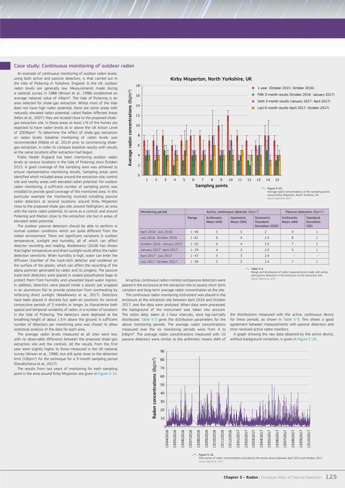
Chapter 5 - Radon | European Atlas of Natural Radiation 125
0
2
4
6
8
10
12
14
16
18
1 2 3 4 5 6 7 8 9 10 11 12 13 14 15
Aver
age
rado
n co
ncen
trat
ions
(Bq/
m3 )
Sampling points
Kirby Misperton, North Yorkshire, UK
1-year (October 2015 - October 2016)
Fi�h 3-month results (October 2016 - January 2017)
Sixth 3-month results (January 2017 - April 2017)
Last 6-month results (April 2017 - October 2017)
0
10
20
30
40
50
60
70
80
90
13/0
4/20
16
13/0
5/20
16
13/0
6/20
16
13/0
7/20
16
13/0
8/20
16
13/0
9/20
16
13/1
0/20
16
13/1
1/20
16
13/1
2/20
16
13/0
1/20
17
13/0
2/20
17
13/0
3/20
17
13/0
4/20
17
13/0
5/20
17
13/0
6/20
17
13/0
7/20
17
13/0
8/20
17
13/0
9/20
17
13/1
0/20
17
Rado
n co
ncen
trat
ions
(Bq/
m3 )
Case study: Continuous monitoring of outdoor radon An example of continuous monitoring of outdoor radon levels,
using both active and passive detectors, is that carried out in the Vale of Pickering in Yorkshire, England. In the UK, outdoor radon levels are generally low. Measurements made during a national survey in 1988 (Wrixon et al., 1998) established an average national value of 4 Bq/m3. The Vale of Pickering is an area selected for shale-gas extraction. Whilst most of the Vale does not have high radon potential, there are some areas with naturally elevated radon potential, called Radon Affected Areas (Miles et al., 2007); they are located close to the proposed shale-gas extraction site. In these areas at least 1 % of the homes are expected to have radon levels at or above the UK Action Level of 200 Bq/m3. To determine the effect of shale-gas extraction on radon levels, baseline monitoring of radon levels was recommended (Kibble et al., 2014) prior to commencing shale-gas extraction, in order to compare baseline results with results at the same locations after extraction had begun.
Public Health England has been monitoring outdoor radon levels at various locations in the Vale of Pickering since October 2015. A good coverage of the sampling area was achieved to ensure representative monitoring results. Sampling areas were identified which included areas around the extraction site, control site and nearby areas with elevated radon potential. For outdoor radon monitoring, a sufficient number of sampling points was installed to provide good coverage of the monitored area. In this particular example the monitoring involved installing passive radon detectors at several locations: around Kirby Misperton close to the proposed shale-gas site; around Yedingham, an area with the same radon potential, to serve as a control; and around Pickering and Malton close to the extraction site but in areas of elevated radon potential.
The outdoor passive detectors should be able to perform in normal outdoor conditions which are quite different from the indoor environment. There are significant variations in outdoor temperature, sunlight and humidity, all of which can affect detector recording and reading. Wasikiewicz (2018) has shown that higher temperature and direct sunlight could affect the radon detection sensitivity. When humidity is high, water can enter the diffusion chamber of the track-etch detector and condense on the surface of the plastic, which can affect the recording of the alpha particles generated by radon and its progeny. The passive track-etch detectors were placed in sealed polyethylene bags to protect them from humidity and unwanted liquid water ingress. In addition, detectors were placed inside a plastic pot wrapped in an aluminium foil to provide protection from overheating by reflecting direct sunlight (Wasikiewicz et al., 2017). Detectors have been placed in discrete but open-air positions for several consecutive periods of 3 months or longer, to characterise both spatial and temporal variability of radon, in a number of locations in the Vale of Pickering. The detectors were deployed at the breathing height of about 1.5 m above the ground. A sufficient number of detectors per monitoring area was chosen to allow statistical analysis of the data for each area.
The average radon levels measured at all sites were low, with no observable difference between the proposed shale-gas extraction site and the controls. All the results from the first year were slightly higher to those measured in the UK national survey (Wrixon et al., 1998), but still quite close to the detection limit (5 Bq/m3) for the technique for a 3-month sampling period (Daraktchieva et al., 2017).
The results from two years of monitoring for each sampling point in the area around Kirby Misperton are given in Figure 5-15.
An active, continuous radon monitor and passive detectors were placed in the enclosure at the extraction site to assess short-term variation and long-term average radon concentration at the site.
The continuous radon monitoring instrument was placed in the enclosure at the extraction site between April 2016 and October 2017, and the data were analysed. When data were processed, the background of the instrument was taken into account. The radon data, taken at 1-hour intervals, were log-normally distributed. Table 5-3 gives the distribution parameters for the above monitoring periods. The average radon concentrations measured over the six monitoring periods were from 4 to 6 Bq/m3. The average radon concentrations measured with 10 passive detectors were similar to the arithmetic means (AM) of
the distributions measured with the active, continuous device for these periods, as shown in Table 5-3. This shows a good agreement between measurements with passive detectors and time-resolved active radon monitors.
A graph showing the raw data obtained by the active device, without background correction, is given in Figure 5-16.
Monitoring period Active, continuous detector (Bq/m3) Passive detectors (Bq/m3)
Range Arithmetic Mean (AM)
Geometric Mean (GM)
Geometric Standard Deviation (GSD)
Arithmetic Mean (AM)
Standard Deviation (SD)
April 2016 - July 2016 1 - 46 5 5 2 4 1
July 2016 - October 2016 1 - 81 6 4 2.4 8 1
October 2016 - January 2017 1 - 50 6 4 2.5 7 1
January 2017 - April 2017 1 - 29 4 3 2.3 5 1
April 2017 - July 2017 1 - 47 5 3 2.4 - -
July 2017 - October 2017 1 - 38 5 3 2.4 7 1
Figure 5-15.Average radon concentrations at the sampling points around Kirby Misperton, North Yorkshire, UK.Source: Ward et al. 2017.
Figure 5-16.Time series of radon concentrations recorded by the active device between April 2016 and October 2017.Source: Ward et al., 2017.
Table 5-3.Range and distribution of radon measurements made with active and passive detectors in the enclosure on the extraction site.Source: Ward et al., 2017.

European Atlas of Natural Radiation | Chapter 5 - Radon126
Radon
5.4. Indoor radon
5.4.1 Introduction
Indoor radon is the most important source of radiation exposure to the public and the second-most common cause of lung cancer after smoking (UNSCEAR, 2008; WHO, 2009). Outdoor radon levels are generally low, but indoor radon concentration can increase significantly since radon tends to accumulate in confined spaces such as buildings. The doses from radon gas when inhaled by humans are two orders of magnitude lower than those received from its progeny. Alpha particles emitted from short-lived, solid radon progenies damage the bronchial regions of the lung. Hence the health effect from radon inhalation is the formation of carcinomas primarily in the bronchial airways (ICRP, 2017).
Long-term exposure to radon has been correlated with the probability of lung cancer (Krewski et al., 2005; Darby et al., 2005; WHO, 2009). Epidemiological studies of underground miners provided the first evidence that exposure to high radon concentrations could be associated with an increased risk of lung cancer, both for smokers and non-smokers (UNSCEAR, 2008; WHO, 2009). Furthermore, results from pooled analyses of general population data collected in Europe, North America and China revealed that exposure to indoor radon, even at low concentration, can be associated with lung cancer (Lubin et al., 2004; Darby et al., 2005, 2006; Krewski et al., 2006).
National and regional radon programmes have been initiated in many countries to reduce risk to the population. The key objectives of radon surveys for targeting residential exposure are (ICRU, 2015; WHO, 2009; IAEA, 2013):• To obtain the distribution of the annual average radon
concentration for a country or an area;
• To study seasonal variation and consider seasonal correction factors to determine the annual average radon concentration;
• To identify areas with elevated radon potential, so-called radon priority areas (RPAs). Clear goals, appropriate design and measurement techniques
have been identified as essential components of any radon survey. The main aspects that should be considered when planning radon surveys include the following (Font, 2009):• To define the objective of the survey;
• To identify the targeted population;
• To choose an appropriate sampling design;
• To allocate resources, budget, staff, data-processing facilities;
• To choose appropriate radon detectors;
• To define the time schedule;
• To choose data-collection methods and questionnaire design.National surveys are, in general, designed for statistical
analysis based on the selected sampling methodology (see Section 2.4). Long-term radon measurements are preferable in order to average out short-term variations (Steck, 2005; Hansen et al., 2014).
Various types of spatial partitioning are used to analyse the data and present maps. Boundaries between spatial units can be administrative, geological or arbitrary (but regular) divisions, such as grid square. Nevertheless, as pointed out by Dubois et al. (2010), there are uncertainties in the indoor radon measurements inside the area boundaries mainly due to the true variability of radon concentration within the spatial unit, the number of observations in the unit and the uncertainties related to seasonal variability of indoor radon concentrations.
Indoor radon mappingRadon is present in every soil type at low levels; however,
certain geographic areas are more prone to high indoor radon concentration than others (McColl et al., 2015). The goal of indoor radon mapping is therefore to delineate radon priority areas. A detailed discussion of radon priority areas is given in Section 5.4.5. The characterisation of indoor radon distributions is to estimate the burden of disease attributable to radon exposure (i.e. lung cancer) on the general population, and to inform government policy in order to reduce the exposure to natural radioactivity
(Gray et al., 2009).The European Basic Safety Standards Directive (European Union
2013) requires that: 'Member states shall identify areas where the radon concentration (as an annual average) in a significant number of buildings is expected to exceed the relevant national reference level', and establishes that a national indoor radon reference level should not be higher than 300 Bq/m3 (see Section 1.2).
Protection activities should be prioritised in these areas (i.e. radon priority areas, RPAs); however, since there are no safe indoor radon levels and even low levels may have adverse health effects (Darby et al., 2005), protective measures should continue to be implemented everywhere (Bochicchio et al., 2017) according to the principle of optimisation on which the system of radiation protection is based (European Union, 2013; see Section 2.1)
The main advantage of indoor over geogenic radon maps is that radon is measured at the exposure point (i.e. dwellings, workplaces). However, map accuracy may be hampered by uncertainties in the location of the test sites, and by unsampled areas (Elío et al., 2017c). Furthermore, indoor radon has high spatial and temporal variability, and depends on multiple factors which are not easily quantified (Tollefsen et al., 2014; Gunby et al., 1993; Borgoni et al., 2014). Finally, data interpretation also requires a correct sample design (Burke & Murphy, 2011) and must take into account possible effects caused by preventive and/or remediation activities (e.g. Long et al., 2013; Finne et al., 2018).
Radon maps form the base for any radon strategy aimed to reduce exposure to this carcinogen, and have therefore profound economic and social implications (Gray et al., 2009). For example, radon maps could be helpful to intensify radon concentration measurements in areas where it is more likely to find buildings with high radon levels. Furthermore, they help to define areas where preventive measures should be installed in new buildings (McColl et al., 2015), although some basic preventive measures in all new buildings (instead of buildings in selected areas only) can be more cost-effective (Gray et al., 2009). In addition, they may also be used to build public awareness (Sainz Fernández et al., 2016).
Indoor radon concentration has high variability at small scale, and even two neighbouring houses may have indoor radon concentrations that differ by some orders of magnitude (e.g. McColl et al., 2015; US-EPA, 2001). The only way to know if a dwelling has a problem with radon is therefore to test it, and indoor radon maps should not be used for this purpose. In Ireland, for example, it was estimated that approximately 43 % of the population that may live in a house with high indoor radon concentration located in areas classified as 'Non-High Radon Area' (Elío et al., 2017); thus, although radon maps are an essential tool for defining national radon action plans, they are not suitable for evaluating the risk of radon in a specific house or workplace.
Indoor radon measurements form the base for creating indoor radon maps (e.g. Fennell et al., 2002; Ferreira et al., 2016). Then geological information and other factors may be used to improve the map accuracy (e.g. Miles & Appleton, 2005; Ferreira et al., 2016; Pásztor et al., 2016; Bossew, 2014, 2015; Elío et al., 2017) since geology is the main factor controlling indoor radon (Watson et al., 2017; Appleton & Miles 2010). Indoor maps may represent the probability of having an indoor radon concentration higher than a national reference level (RL) (e.g. Fennell et al., 2002; Miles et al., 2007), or an average indoor radon concentration over large areas (e.g. Friedmann, 2005; Dubois, 2005). Recent studies, however, have also included the potentially adverse health effects of radon exposure (i.e. by estimating the number of lung cancers attributable to radon in a given area) and population density for defining radon priority areas (Elío et al., 2018).
The criteria selected to delineate RPAs therefore depend on national radiological protection strategies and the data available, and even multiple criteria may be applied in parallel to optimise a radon action plan (Elío et al., 2018). However, different strategies may lead to contradictory information, and it is common that RPAs do not match across borders. In this respect, for example, Ireland defines RPAs as areas where the probability of having an indoor radon concentration higher that the reference level of 200 Bq/m3 is 10 % or higher (Fennell et al., 2002), whereas the threshold in Northern Ireland is 1 % despite having the
same reference level (Daraktchieva et al., 2015). Map resolution may also vary between countries, i.e. grids of 10 km × 10 km in Ireland and 1 km × 1 km in Northern Ireland. Table 5-5 presents a summary of different methods to map radon.
In France, Ielsch et al. (2010) developed a methodology to derive a map of the geogenic radon potential by determining the capacity of geological units to produce radon based on their uranium content. This initial map was then improved by taking into consideration major fault lines and underground mines, which control the preferential pathways of radon through the ground. Kropat et al. (2015) used Kernel regression to map indoor radon concentration in Switzerland. The maps were produced taking into account building styles and geology.
5.4.2 Materials and methods for indoor radon measurements
WHO (2009), IAEA (2013) and Bartzis et al. (2018) provide guidance on requirements for radon measurements in homes. The measurements should permit assessment of mean annual radon concentration; the measurement protocols should be standardised to ensure consistency of results; the detector type should be chosen carefully; and quality assurance and controls should be pursued in order to ensure reliability of the measurements.
It is well known that radon progeny is responsible for most of the radiation dose. Devices that measure radon progeny are excluded from this discussion because they are quite complicated to use and are not practical for estimating radon levels in dwellings. Notably, dose from radon progeny strongly depends on the aerosol size distribution, and, for the typical range of aerosol distributions that can be found in a dwelling, dose can be considered proportional to radon concentration. (e.g. Hopke et al., 1995). Only measurements of radon gas are considered in this section.
Radon measurements in dwellings are discussed in terms of the duration of the tests and the type of instrument used. The duration could range from a few days to several months, while the instrument could be passive or active. When an air sample is taken by pumping air into the measuring volume, the device is called active; whereas when air enters the measuring chamber by diffusion, the instrument is called passive. Section 2.5 describes the different devices in more detail.
Estimating the number of dwellings above the reference level
Different techniques have been developed to estimate the number of dwellings exceeding action or reference levels. A log-normal model of indoor radon concentration can be used to estimate the proportion of the probability distribution above the reference or action level. The procedure explained by Miles (1998) involves subtracting the outdoor radon concentration from the measured indoor values and taking the natural logarithm, i.e. ln(Ri - Ro), where Ri and Ro are indoor and outdoor radon concentrations, respectively. The outdoor radon value to be subtracted can be estimated carrying out an analysis of quantile-quantile plot of the data, e.g. Gunby et al. (1993) and Daraktchieva et al. (2014).
Moreover, Antignani et al. (2019) studied the impact of outdoor radon concentration on estimated percentages above some reference levels.
The arithmetic mean and standard deviation of those values may then be calculated. Under the assumption of a normal distribution of ln(Ri - Ro) with mean µ and standard deviation σ, the proportion of dwellings above the reference level, NRL, can be calculated using the standard cumulative distribution function Φ, as follows:
RP
C = A . e . ß . (1 - p) p-1
C∞
(-log10(k) - 10)=
F ARa D0
0.75
. ρb .
.
λ p exp(-6 Sp - 6S14p)
D0 exp(-6 Sp - 6S14p)
J2
(m + λ222 . Co) . V
S
. ε .
. ε .
T273( )= √
(
[ ]( )
)
FTn ARa-224 ρb λTn
. e-λt . (1 - e-λt )
(C - C0e-λt )
S(1 - e-λt )
+
=
E222=
E0=
NRL=
δA δa12 + δa2
2 + δa32 + .. . + δan
2
2(Measured Mean - Reference Value
Reference Value
=
D
WL = EEC (Bq /m3)/3 700 = F *CRn (Bq /m3)/3 700
PAEE(WLM) = PAEC(WL) *
DC * EEC * t DC * F * t * CRn=
% PME × 100 +=
=
λ 220 . V0
-λ . (V / Q)220 1S
Cm
eE220
E222
=
λ . V
λ . V
1 - Φ 12 σ2x
1 - eln (Ri - R0) - µ
σ
( )Exposure (h)170
[ ]( )2
Standard Deviation
Measured Mean× 100
Ct C0=
√
√
√
-(x-µ)2
2σ2 -(x-µ)2
2σ2-∞
i 0ln (R - R )
∫
(5-1)
(5-2)
(5-4)
(5-5)
(5-7)
(5-8)
(5-9)
(5-6)
(5-10)
(5-11)
(5-12)
(5-13)
(5-14)
(5-3)√
√
NAPL Pi =−J ± −4CH
2H
π
More sophisticated techniques have been developed to reduce the influence of extreme values on the sample mean and sample standard deviation. Miles (1994) applied a sorting technique to calculate the geometric mean (GM) and geometric standard deviation (GSD). Miles and Appleton (2005) showed that Bayesian estimates of the GSD could be used to improve estimates in areas where data are scarce.
A reminder222Rn is called radon (Rn).220Rn is called thoron (Tn).
Chapter 5 - Radon | European Atlas of Natural Radiation 127
Country (region) Reference Level* (Bq/m3) Objectives Methods Resolution Reference
Austria 200 and 400 Divide the country into three classes: i.e. average annual concentration <200, 200 - 400, and >400 Bq/m3
Annual mean radon concentration in a standard situation
Administrative level (i.e. municipality)
Friedmann (2005)
Bayesian statistics, combining indoor radon measurements (standard situation) and geology
Geological classes (scale 1:500 000)
Friedmann & Gröller (2010)
Azerbaijan 200 Display the indoor radon concentration values Arithmetic mean of indoor radon gas concentration values
10 km × 10 km and district Hoffmann et al. (2017)
Belgium (Walloon region) 400 Percentage of dwellings above the RL taking into account geological information
Moving average between geological units
1 km × 1 km Cinelli et al. (2011)
Hungary 200 Percentage of standard houses (i.e. one-storied, no basement houses) above the RL. Also reports the arithmetic mean and the maximum value
Lognormal model Various: Administrative level (i.e. counties), and grids 10 km × 10 km
Minda et al. (2009)
Ireland 200 Percentage of houses above the RL based solely on indoor radon measurements RPA when P[InRn > RL] ≥ 10 %
Lognormal model Grids 10 km × 10 km Fennell et al. (2002)
200 Percentage of houses above the RL based on indoor radon and geological information (i.e. bedrock geology, Quaternary geology, subsoil permeability, and soil permeability). RPA when P[InRn > RL] ≥ 10 %
Logistic regression model Grids 1 km x 1 km Elío et al. (2017)
- Estimation of radon-related lung cancer cases Dose estimation based on average concentrations (i.e. block averages after ordinary kriging)
Administrative level (i.e. electoral division)
Elío et al. (2018)
Italy (Abruzzi region)
100, 200 and 300 Risk that a standard house exceeds the RL. Divide the country into seven categories.
Bayesian spatial quantile regression, and Bayesian model for spatial cluster detection
Administrative level Sarra et al. (2016)
Italy (Lombardy region)
200 and 400 Percentage of houses above the RLs. RPA when the RL (200 or 400 Bq/m3) is below the lower confidence limit at 95 % of the quantile 0.9 (P[InRn > RL] ≥ 10 %).
Geostatistical simulation (i.e. multi-Gaussian sequential simulation).
Administrative level (i.e. electoral division)
Borgoni et al. (2010)
Malta 100 Display the indoor radon concentration values Average of geometric mean annual indoor radon gas concentration values for each sampling point
Grids 5 km × 5 km Baluci et al. (2013)
North Macedonia 100 and 200 Display the probabilities of having an indoor radon concentration higher than 100 and 200 Bq/m3, and the expectation.
Estimations are derived from 226Ra concentration in soil
Grids 5 km × 5 km Bossew et al. (2013)
Norway 200 Percentage of houses above the RL based on indoor radon and geological information (bedrock and Quaternary geology). RPA when P[InRn > RL] ≥ 20 %.
Classify geological polygons according to local (polygon) statistics or national (class) statistics
Geological polygons Watson et al. (2017)
Spain 300 Identify 3 radon classes Model that uses as input data: national indoor radon databases; natural γ-radiation map (MARNA); geological maps
Geological unit García-Talavera et al. (2013)
Switzerland 100 and 300 Percentage of homes having an indoor radon concentration <100, 100 - 300, and >300 Bq/m3
Ordered logistic regression model
Grids 10 km × 10 km Kropat et al. (2017)
United Kingdom 200 Percentage of houses above the RL taking into account geological information. RPA when P[InRn > RL] ≥ 1 %
Lognormal model, corrections to account for year-to-year and random variations (i.e. Bayesian statistics)
Grids 1 km × 1 km Miles et al. (2007); Miles et al. (2011); Daraktchieva et al. (2015)
* Reference Level (RL) reported in the cited papers, not referring to the RL in the Basic Safety Standards Directive (European Union, 2013).
Details on the most commonly used passive devicesTrack-etch detectors are passive instruments that use plastic as
detector material. The plastic can be a polyallyl-diglycol carbonate (PADC), cellulose nitrate (LR-115), or polycarbonate (Makrofol). The alpha particles generated by radon or radon decay products damage the surface of the plastic material and produce latent tracks. These tracks are made visible by chemical or electrochemical etching which enlarges the size of the alpha tracks, making them observable by light microscopy so that they can be counted by an automated counting device. The number of tracks per unit surface area, after subtracting background counts, is directly proportional to the radon exposure in kBq h/m3. A conversion factor obtained by controlled exposure at a calibration facility allows conversion from track density to radon concentration (Nikezic & Yu, 2004). The placement and collection protocols should be followed very carefully to obtain the best results.
There are two types of track-etch detectors: open (the plastic material is exposed to the ambient atmosphere) and closed (the material is enclosed in a container). Open track-etch detectors record alpha particles originating from radon decay products and from all radon isotopes. For these
detectors the equilibrium factor F should be taken into account to estimate the number of alpha particles from radon decay only. Closed track-etch detectors allow only radon to diffuse into the closed diffusion chamber and therefore exclude the entry of ambient radon decay products. Passive track-etch detectors are not sensitive to background beta and gamma radiation.
Activated charcoal detectors are passive detectors that are used for short-term measurements of indoor radon. An airtight container with activated charcoal should be opened and placed in the measured place for 1 to 7 days. The containers could be open-faced or equipped with a diffusion barrier to extend the sampling period up to 7 days. At the end of the sampling period, the container should be sealed so that the radon decay products equilibrate with the radon collected. Detectors should be returned for analysis as soon as possible after the exposure period because of the short half-life of radon of 3.8 days. Since the response of activated charcoal detectors is affected by humidity, detectors should be calibrated to various levels of humidity. Because charcoal allows continuous adsorption and desorption of radon, the method only provides a good estimate of the
average radon concentration during the exposure time if changes in radon concentration are small. The use of a diffusion barrier reduces the effects of draughts and high humidity.
Electrets are passive detectors that use an electrostatically charged disk to measure radon concentrations. The electret is situated within a small ionisation chamber. Radon diffuses through a filter into the chamber, and the charged alpha particles emitted by radon and its decay products ionise the air within the chamber volume. The negative ions are collected by the positive electret located at the bottom of the chamber. Radon concentration is proportional to the voltage drop in the electret. There are short-term and long-term electret detectors. Short-term detectors could be placed for 2 to 7 days sampling, while long-term detectors could be used for up to 12 months. The background gamma radiation during exposure could affect measurements, so results should be corrected for it (RadElec E-Perm, 2008).
Table 5-5.Examples of different methodologies for mapping radon.

European Atlas of Natural Radiation | Chapter 5 - Radon128
Radon
A survey conducted by WHO (2007) revealed that the most popular passive radon measuring devices are track-etch detectors, activated charcoal detectors and electrets. In Europe, track-etch detectors certainly dominate.
Long-term sampling (from several months to a year) of the average radon concentration is generally performed using passive radon detectors. Although short-term sampling, lasting a few days only, could be used, it is not recommended for assessing the mean annual radon concentration. Indoor radon concentration exhibits diurnal, monthly and seasonal variations (Miles & Algar, 1998; Miles, 2001; Wrixon et al., 1998) as well as significant short-term fluctuations. To account for these variations, long-term sampling over several months is required. Radon variability is higher over shorter exposure periods (ICRU Report 88; ICRU, 2015).
In dwellings, radon detectors should be placed according to standard protocols for deployment and collection of detectors (IAEA, 2013; Bartzis, 2018; Daraktchieva et al., 2018). Some countries use trained personnel to place detectors, while others send detectors by post with detailed instructions on how and where to place the detectors. For example, Public Health England provides guidance to houseowners on indoor radon monitoring; see http://www.ukradon.org/information/measuringradon. The measurement protocol schedule should be appropriate for the purpose of estimating the mean annual radon concentration.
The radon concentration measured in a given place of a particular dwelling varies with time. Climate influences the amount of gas emanating from the Earth, both through air pressure and outdoor temperature. Ideally, radon should be measured in all the inhabited rooms of a dwelling in order to estimate the mean annual radon concentration that represents radon exposure of the occupants in the dwelling. This is impractical, however, so measurements are usually made in two rooms with the highest occupancy rates, typically a bedroom and a living room. Some countries measure radon in only one room situated on the ground floor. In such cases, radon concentration is probably overestimated if the dwelling has more than one floor (see Section 5.4.5). It has been shown that temperature, direct sunlight and humidity could affect detector sensitivity (Hardcastle & Miles, 1996; Moreno et al., 2013; Venoso et al., 2016; Wasikiewicz, 2018). Higher temperatures could affect radon detection sensitivity, resulting in over-readings of the integrated radon exposure. Moreover, exposing the diffusion chamber to direct sunlight would also have an adverse effect on radon measurements. In a wet environment, water can enter the diffusion chamber of the track-etch detector and condense on the surface of the PADC element, which results in an underestimation of the exposure. Therefore, detectors should be placed in areas that are far away from heat sources, direct sunlight and high humidity. For example it is recommended that detectors should be placed at least 10 cm from the wall in the normal breathing zone and away from small children and pets. The detectors should be used in normal living and ventilation conditions, and performing sampling in sealed or inhabited rooms should be avoided.
Uncertainties associated with radon exposure assessment
Indoor radon measurements with passive track-etch detectors, which are the most popular choice, are associated with uncertainties that need to be investigated and quantified. Two types of uncertainties are associated with radon exposure assessment: they are called classical and Berkson-type errors (Heid et al., 2004). The classical-type errors are statistically independent of the true variable, while the Berkson-type errors (Berkson, 1950) are statistically independent of the observed variable. The classical errors arise when values, obtained by repeated measurements, vary around the true value. The Berkson errors arise when the group average value is used instead of individual values and the true value varies randomly around the measured value. The classical-type errors can be quantified, analysed and minimised by appropriate measures, while the Berkson-type errors cannot easily be quantified but can be identified and modelled.
The typical laboratory uncertainties belong to the classical errors because they can be measured and quantified. These are (Miles et al., 1997; Ibrahimi et al., 2009):
• Uncertainties in the radon calibration reference valueIn general, radon detectors are calibrated against a standard
radon source or more frequently against a transferred standard. The transferred standard is a reference instrument which is calibrated against a standard radon source. The estimated uncertainty of the reference instruments can vary for different laboratories with a typical value between 6 % and 10 %.
• Variations in track-etch materialsTrack-etch materials are commercially available with quality
of the material varying from supplier to supplier and from manufacturing batch to manufacturing batch. Hanley et al. (2008) calculated that the typical between-sheet variability yielded 2.1 % uncertainty. The processing laboratory should therefore implement rigorous quality-assurance control in order to identify the variation in the material and introduce correction measures.
• Uncertainties due to variation in the etching processVariations in etching conditions can alter track sizes.
Therefore, etching parameters, such as temperature, etching time and chemical composition and concentration of etchant, should be monitored and kept the same (Miles, 1992, 2004). The uncertainties associated with the etching process can be measured using a control sample of detectors.
• Uncertainties of the automatic track counting systemInconsistent focusing and reading of the track-etch detectors
can lead to misinterpretation of the track-etch characteristics. The focus of the counting system may drift, the track recognition may change and the scratches or the surface defects may deteriorate the signal-to-background ratio, thus increasing the measurement uncertainty. The combined uncertainty of the automatic track counting system is estimated to be 5.5% (Hanley et al., 2008).
• Uncertainties in the linearity of responseThe detectors are exposed to a wide range of radon
concentrations, varying from 20 (or even lower) to several thousands of Bq/m3. When exposure is high, more alpha particles damage the material. Therefore, the probability of a new track to lay down on top of a previous track is higher. When the tracks start to overlap, the calibration curve, which is the number of tracks as a function of radon concentrations, becomes non-linear, and a correction factor should be considered. The required degree of linearity correction depends on the size of the etched tracks.
• Uncertainties due to chemical change of the track-etch material: ageing and fadingTrack-etch materials are subject to many changes and
variations with time. Hardcastle and Miles (1996) showed that the polymer sensitivity of CR-39 to alpha radiation damage decreases over time due to ageing (i.e. the increases in cross-linking of the polymer) and fading (the partial repair of damaged trails over time). Reduction in radon sensitivity from both ageing and fading is responsible for underestimation of radon activity concentrations. As detectors are placed for a minimum of three months during a sampling, they are subject to both ageing and fading effects. The estimated uncertainties due to aging and fading given by Hanley et al. (2008) are 4.5 % and 4.4 %, respectively. However, the ageing and fading effect depends on the technique, including the readout system (both hardware and software) and that in some cases ageing and fading do not affect the detector sensitivity (Calamosca & Penzo, 2008).
The laboratory uncertainties can be estimated by identifying and measuring all known errors contributing to the total error δA and calculate the total uncertainty using the square root of the sum of squared errors. The quantities a1, a2, a3, ..., an are assumed to have uncorrelated and random errors δa1, δa2, δa3, ..., δan, respectively. In this case, the uncertainties add in quadrature:
RP
C = A . e . ß . (1 - p) p-1
C∞
(-log10(k) - 10)=
F ARa D0
0.75
. ρb .
.
λ p exp(-6 Sp - 6S14p)
D0 exp(-6 Sp - 6S14p)
J2
(m + λ222 . Co) . V
S
. ε .
. ε .
T273( )= √
(
[ ]( )
)
FTn ARa-224 ρb λTn
. e-λt . (1 - e-λt )
(C - C0e-λt )
S(1 - e-λt )
+
=
E222=
E0=
NRL=
δA δa12 + δa2
2 + δa32 + .. . + δan
2
2(Measured Mean - Reference Value
Reference Value
=
D
WL = EEC (Bq /m3)/3 700 = F *CRn (Bq /m3)/3 700
PAEE(WLM) = PAEC(WL) *
DC * EEC * t DC * F * t * CRn=
% PME × 100 +=
=
λ 220 . V0
-λ . (V / Q)220 1S
Cm
eE220
E222
=
λ . V
λ . V
1 - Φ 12 σ2x
1 - eln (Ri - R0) - µ
σ
( )Exposure (h)170
[ ]( )2
Standard Deviation
Measured Mean× 100
Ct C0=
√
√
√
-(x-µ)2
2σ2 -(x-µ)2
2σ2-∞
i 0ln (R - R )
∫
(5-1)
(5-2)
(5-4)
(5-5)
(5-7)
(5-8)
(5-9)
(5-6)
(5-10)
(5-11)
(5-12)
(5-13)
(5-14)
(5-3)√
√
NAPL Pi =−J ± −4CH
2H
π
Typical Berkson-type errors related to the radon exposure of the inhabitants and not to the radon measurements are:
• Uncertainties in the results due to people’s behaviour in the monitoring premisesRadon monitors are placed in peoples’ homes for several
months. The measuring laboratory provides instructions for placing detectors. The exposure period is calculated from the information provided by the houseowner. The annual radon concentration is calculated according to the typical behaviour of people living in the house during the period of measurement. However, people may alter their behaviour during the monitoring period, for example by increasing or decreasing a ventilation rate of the house, compared to their usual behaviour. Such a change in ventilation rate (or non-occupation of the house during the measurement period) may undermine the results from the detectors, and therefore make them unrepresentative.
Further uncertainties can be attributed to variations of conditions during the exposure period. For example, a building may only be occupied for a part of the day or a part of the week, but detectors record constantly the radon concentration in the building.
• Uncertainties due to spatial variation between radon activity concentrations of rooms in the dwelling. Variation in radon concentration in different rooms of the same
house increases the overall uncertainty of the estimated radon exposure. This is the case especially when only one room has been measured. However the average radon concentration over two rooms is also affected by this source of uncertainty. Radon monitors are usually placed in the two most occupied rooms. The uncertainties arise from the fact that radon concentration in unsampled rooms may differ from that in the monitored rooms, which are used as a substitute for the concentration in the other rooms.
The radon concentration differences are higher between different floors as compared with detectors on the same floor. A coefficient of 30 % has been used as the best estimate of the error in exposure estimates due to variations of radon activity concentration between rooms (Heid et al., 2004). Much lower variation (about 10 % on average) was found in another study (FIsher et al., 1998), especially between rooms located on the same floor.

Chapter 5 - Radon | European Atlas of Natural Radiation 129
5.4.3 The European Indoor Radon MapIn 2005 the JRC published an overview of radon surveys conducted
by that time in some 30 European countries (Dubois, 2005). It showed that no two countries had used the same approach, in terms of survey design, measurement techniques and mapping strategies. With such differences in the choice of mapped quantity and in type of visualisation, the resulting maps were heterogeneous and incompatible across borders, so that collating them on a European scale resulted in no more than a colourful patchwork.
The Euratom Treaty, mainly its Article 39 (European Union, 2016), gives the JRC the mandate to collect, present, evaluate and interpret radiological data from the EU Member States. With this in mind, in 2006 the JRC decided to create a European map of indoor radon concentration. As the above survey (Dubois, 2005) showed, indoor radon measurements were already available from most European countries; however, collecting this information from different authorities and integrating it into a common framework implied a number of conceptual and technical challenges. The decisive discussions on how to develop a European Indoor Radon Map, including determining a technical procedure, took place at the international radon workshop in Prague in 2006. As a result, both EU and non-Member States participate to the mapping effort. This map was chosen as the first step towards creating a European Atlas of Natural Radiation (Dubois et al., 2010; De Cort et al., 2011).
MethodologyThe European Indoor Radon Map (EIRM) intends to show
'means over 10 km × 10 km grid cells of long-term (ideally, annual means of) indoor radon concentration in ground-floor rooms of dwellings.' The participating countries, involving national competent authorities, laboratories, universities etc., aggregate their raw data into 10 km × 10 km cells over a grid covering Europe. Finally the national competent authorities provide this input data (grid values) to the JRC. For historical reasons, this grid uses the GISCO-LAEA coordinate reference system (spherical Earth, zero-point at 9° E/48° N). Exceptions have been made for Ireland and Malta since they had already used their own 10 km × 10 km grids based on their national coordinate reference systems before participating to the European map.
The size of the grid cells has been chosen as a compromise between contradicting targets: On one hand, a small cell size implies many empty cells and poor cell statistics, since also the spatial resolution of observation is naturally limited (also, in cases of sparsely populated regions, high resolution may reveal information on individual dwellings, which conflicts with the requirement of data protection). On the other hand, small cells would have allowed revealing more local structure of the true radon field, which is lost as cell size increases.
Specifically, the national data providers fill the cells with the following statistics calculated from their original data:• Arithmetic mean (AM);
• Standard deviation (SD);
• AM and SD of the ln-transformed data;
• Median (MED);
• Minimum (Min) and maximum (Max);
• Number of original measurements per cell (N).This procedure was agreed upon to ensure data protection,
because the original data and their exact locations are not given away, but remain at the national level, thus guaranteeing data privacy to houseowners. The methods and procedures to collect and process the raw data have been further described by Dubois et al. (2010) and Tollefsen et al. (2011).
The choice of variable to be mapped can be seen as a compromise between an indoor radon map, which would be a proxy of an exposure map, and a geogenic 'radon potential' map. Since most people in fact do not live in ground-floor rooms and are not exposed continuously (i.e. 24 hours a day, 365 days a year), the mapped variable does not reflect the radon environment to which people are actually exposed. Rather, it shows a standardised indoor concentration, namely restricted to the conditions 'ground floor' and 'annual mean'. On the other hand, the variable still includes anthropogenic factors which influence radon levels, namely building styles and living habits; hence it is not a measure of radon potential, which is defined to include only natural (geogenic), but no anthropogenic, radon controls.
Restricting the data to annual mean radon concentration in ground-floor rooms of dwellings means that data providers have to estimate this quantity, ideally from long-term measurements.
Whenever measurements have been made over shorter time periods, some intermediate modelling involving seasonal corrections may be necessary to estimate annual means. As seasonal variations depend on a number of factors including climate, building styles, occupation and ventilation habits etc., no general model exists for Europe, so estimating this quantity has been entrusted to the national data providers.
As a consequence, the statistics over the chosen quantity do not represent the ones of exposure. For that purpose, detailed information about the population distribution at floor level for each country is necessary. Unfortunately, since such data are not available for all European countries, no radon exposure map could be developed for this Atlas.
Since 2010, the JRC has sent a quality-assurance questionnaire to national data providers, asking them inter alia for information about their survey designs, measurement methods, detectors used and data processing techniques applied. In most of the 20 countries that have responded to this questionnaire, the datasets represent a combination of several studies and surveys, often carried out with different purposes and therefore with different survey designs (Gruber et al., 2013). In addition to radon data collected in dwellings, some participating countries have also provided data for other building types (e.g. workplaces, schools, kindergartens) and in some cases with sampling period less than a full year.
Results and discussionAs of September 2018, 35 European countries participate to
the EIRM, including all the current 28 EU Member States but one. More than 28 000 grid cells have been filled with statistical data, which are in turn based on more than 1 100 000 individual measurements in total; see Table 5.6 for descriptive statistics of the dataset which underlies the map.
As can be seen from the map (Plate 6), the number of measurements per cell and proportional coverage of national territory vary widely between participating countries and between regions of individual countries. The number of measurements per cell ranges from a single one up to a maximum of nearly 24 000 (for a cell in the UK). Still, there are many empty cells. The map may thus be considered to reflect the status of national surveys of indoor radon monitoring in Europe, at least up to the data prepared and released by national authorities to the JRC.
Large areas with high sampling density are found in e.g. South Finland, the Czech Republic, Austria, Switzerland, North Italy, Belgium, Luxembourg, the UK and Northern Ireland. The median number of measurements per cell equals 4, with a median absolute deviation of 4.4 (see Table 5.6). This heterogeneity of
sampling density clearly influences the statistical uncertainty of the means as estimates of the expected concentration within a cell, as it does for the standard deviation and other statistics.
The wide ranges in sampling density depend on the design of the survey from which the data originate.
Some countries have mainly aimed for a homogeneous coverage of their territory, while others (e.g. Austria) have aimed for a population-weighted estimate of the radon concentration, which results in a sampling density essentially proportional to the population density. Five countries (namely Germany, the Czech Republic, Switzerland, Spain and Finland) have carried out more detailed surveys in high-radon areas. Finally, some datasets
(from Greece and Poland) are mainly based on surveys in high-radon areas. As biased sampling influences the statistics, the data are not necessarily representative for the whole countries. For further discussion about representativeness and selected topics of quality assurance, see Section 2.4.7 as well as Bossew et al. (2012).
As seen from the maps, many areas of Europe are still not covered. Although a few uninhabited areas will always remain, other reasons include the following: missing data, because radon surveys are still ongoing; older surveys were conducted without recording precise geographical coordinates of the sampled dwellings; or national surveys have concentrated on high-radon areas.
The next map (Plate 7) shows the geographical distribution of arithmetic means over the grid cells. This map reveals a spatial trend in indoor radon concentration across Europe and essentially reflects the underlying geology. Regions of high radon concentrations are found in the granitic zones of the Bohemian Massif, the Fennoscandian Shield, the Iberian granite province, the Massif Central, Corsica, Cornwall, and the Vosges Mountains; in the crystalline rocks of the Central Alps and karst rocks of the Swiss Jura and the Dinarides; in the black shales of North Estonia; in certain volcanic structures in Central Italy; and in the lower Devonian of Ardennes, where the high radon risk may be caused by the concentration of uranium in weathering products, a result of rock history, not directly connected to its global uranium content. Apart from geology, also climatic and anthropogenic factors contribute, but their spatial structure is not evident and remains to be investigated.
The arithmetic mean of all non-empty cells in Europe (for participating countries) is 103 Bq/m3, while the median is 60 Bq/m3 (see Table 5-6). Note, however, that this spatial mean (mean over cells) is different from the mean over individual measurements (AM = 148 Bq/m3, calculated as the cell arithmetic mean weighted by the number of measurements), from the mean over country-means (AM = 97 Bq/m3) and again, in general, from the population-density-weighted mean (no value available so far).
According to the WHO Handbook on Indoor Radon (WHO, 2009), a national reference level of 100 Bq/m3 is recommended to limit the risk of individuals. Wherever this is not possible, the chosen level should not exceed 300 Bq/m3. In the recently modernised and consolidated Basic Safety Standards Directive (European Union, 2013), a reference level for workplaces and dwellings of at most 300 Bq/m3 is required (see Section 1.2).
For all the countries participating to the EIRM, 34 % of the non-empty cells have an arithmetic mean above 100 Bq/m3 and 4 % of them above 300 Bq/m3 (see Table 5-6). Similarly, exceedance
probabilities have been calculated for each participating country (see Tollefsen et al., 2014, and Cinelli et al., 2018, supplementary material). In the Czech Republic, more than 90 % of the AMs of all non-empty cells exceed 100 Bq/m3. At the other end of the scale, none of the cells in the Netherlands have an AM above this level. Again, these figures can be explained by the underlying geology. However, for countries which had reported data (by September 2018) mainly from high-radon areas (e.g. Greece and Poland), such statistics should be interpreted as only regionally indicative, at least until data with national coverage become available. In any case, this variability demonstrates how differently the countries are affected by the radon problem.
MED, median; MAD, median absolute deviation, MAD(zi) := MED {|zi – MED(zi)|}; AM, arithmetic mean; CV, coefficient of variation, where CV := SD/AM; GSD, geometrical standard deviation. (See also Section 2.4 for definitions.)
Descriptive statistics for the European Indoor Radon Map
Number of non-empty cells 28 468
Total number of measurements 1 158 888
Number of measurements per cell MED ± MAD 4 ± 4.4
Minimum and maximum number of measurements per cell Min/Max 1/23 993
Considering the arithmetic mean of each cell AM ± CV % 103 Bq/m3 ± 138 %
Considering the median of each cell MED ± MAD 60.0 ± 45.5 Bq/m3
Percentage of cells with AM > 300 Bq/m3 4.24%
Percentage of cells with AM > 100 Bq/m3 34.1%
Considering the CV (%) of each cell MED ± MAD (65.5 ± 34.9) %
Considering the GSD of each cell MED ± MAD 1.87 ± 0.68
Table 5-6.Descriptive statistics for the dataset on which the EIRM is based, as of September 2018.Source: EANR, EC-JRC, 2019.
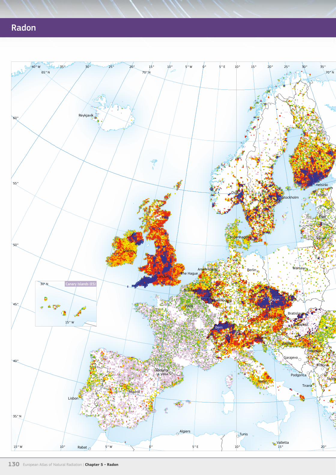
European Atlas of Natural Radiation | Chapter 5 - Radon130
0 ° 5 ° E 10 ° 15 ° 20 ° 25 ° 30 ° 40 ° E5 ° W10 °
0 ° 5 ° E 10 ° 15 °15 ° 20 °20 ° 25 °25 ° 30 °30 ° 35 °35 ° 40 °40 ° W 45 ° 50 ° 55 ° 60 ° 65 ° 70 ° E5 ° W10 °
15 ° W
35 ° N
40 °
45 °
50 °
55 °
60 °
35 ° N
40 °
45 °
50 °
55 °
60 ° N65 ° N 65 ° N70 ° N 70 ° N
15 ° W
30° N
Reykjavík
Andorrala Vella
Brussels
Amsterdam
Dublin
The HagueLondon
Berlin
Copenhagen
OsloStockholm
Tallinn
Helsinki
VilniusMinsk
WarsawKiev
Moscow
Chişinău
Bucharest
Ankara
Nicosia
Cairo
BeirutDamascus
Baghdad
Baku
Yerevan
Tbilisi
‘Ammān
Jerusalem
Tel Aviv-Yafo
Athens
Belgrade
ViennaBratislava
Prague
Bern
Luxembourg
Paris
RomeTirana
Podgorica
Sarajevo
Priština
Skopje
Sofia
Madrid
Zagreb
Ljubljana
Budapest
Valletta
Tripoli
TunisAlgiers
Rabat
Lisbon
Riga
Canary Islands (ES)
Radon
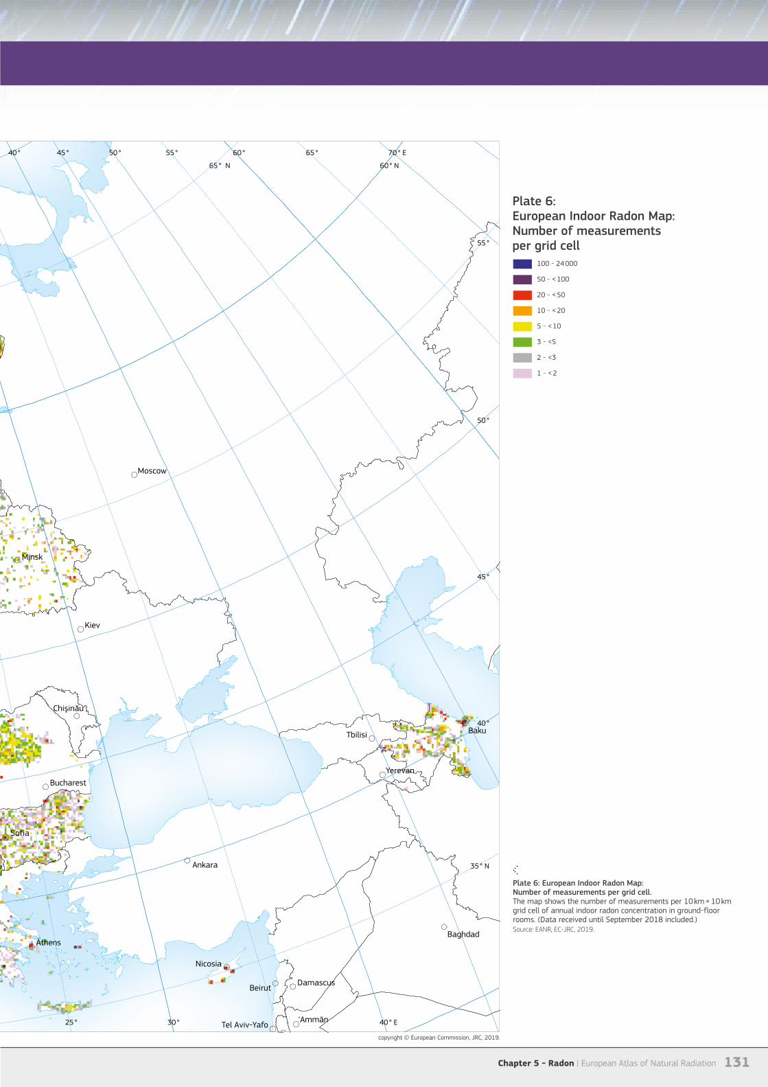
Chapter 5 - Radon | European Atlas of Natural Radiation 131
0 ° 5 ° E 10 ° 15 ° 20 ° 25 ° 30 ° 40 ° E5 ° W10 °
0 ° 5 ° E 10 ° 15 °15 ° 20 °20 ° 25 °25 ° 30 °30 ° 35 °35 ° 40 °40 ° W 45 ° 50 ° 55 ° 60 ° 65 ° 70 ° E5 ° W10 °
15 ° W
35 ° N
40 °
45 °
50 °
55 °
60 °
35 ° N
40 °
45 °
50 °
55 °
60 ° N65 ° N 65 ° N70 ° N 70 ° N
15 ° W
30° N
Reykjavík
Andorrala Vella
Brussels
Amsterdam
Dublin
The HagueLondon
Berlin
Copenhagen
OsloStockholm
Tallinn
Helsinki
VilniusMinsk
WarsawKiev
Moscow
Chişinău
Bucharest
Ankara
Nicosia
Cairo
BeirutDamascus
Baghdad
Baku
Yerevan
Tbilisi
‘Ammān
Jerusalem
Tel Aviv-Yafo
Athens
Belgrade
ViennaBratislava
Prague
Bern
Luxembourg
Paris
RomeTirana
Podgorica
Sarajevo
Priština
Skopje
Sofia
Madrid
Zagreb
Ljubljana
Budapest
Valletta
Tripoli
TunisAlgiers
Rabat
Lisbon
Riga
100 - 24 000
50 - < 100
20 - < 50
10 - < 20
5 - < 10
3 - <5
2 - <3
1 - < 2
Plate 6: European Indoor Radon Map:Number of measurementsper grid cell
Plate 6: European Indoor Radon Map:Number of measurements per grid cell.The map shows the number of measurements per 10 km × 10 km grid cell of annual indoor radon concentration in ground-floor rooms. (Data received until September 2018 included.)Source: EANR, EC-JRC, 2019.
copyright © European Commission, JRC, 2019.

European Atlas of Natural Radiation | Chapter 5 - Radon132
0 ° 5 ° E 10 ° 15 ° 20 ° 25 ° 30 ° 40 ° E5 ° W10 °
0 ° 5 ° E 10 ° 15 °15 ° 20 °20 ° 25 °25 ° 30 °30 ° 35 °35 ° 40 °40 ° W 45 ° 50 ° 55 ° 60 ° 65 ° 70 ° E5 ° W10 °
15 ° W
35 ° N
40 °
45 °
50 °
55 °
60 °
35 ° N
40 °
45 °
50 °
55 °
60 ° N65 ° N 65 ° N70 ° N 70 ° N
15 ° W
30° N
Reykjavík
Andorrala Vella
Brussels
Amsterdam
Dublin
The HagueLondon
Berlin
Copenhagen
OsloStockholm
Tallinn
Helsinki
VilniusMinsk
WarsawKiev
Moscow
Chişinău
Bucharest
Ankara
Nicosia
Cairo
BeirutDamascus
Baghdad
Baku
Yerevan
Tbilisi
‘Ammān
Jerusalem
Tel Aviv-Yafo
Athens
Belgrade
ViennaBratislava
Prague
Bern
Luxembourg
Paris
RomeTirana
Podgorica
Sarajevo
Priština
Skopje
Sofia
Madrid
Zagreb
Ljubljana
Budapest
Valletta
Tripoli
TunisAlgiers
Rabat
Lisbon
Riga
Canary Islands (Spain)
Radon

Chapter 5 - Radon | European Atlas of Natural Radiation 133
0 ° 5 ° E 10 ° 15 ° 20 ° 25 ° 30 ° 40 ° E5 ° W10 °
0 ° 5 ° E 10 ° 15 °15 ° 20 °20 ° 25 °25 ° 30 °30 ° 35 °35 ° 40 °40 ° W 45 ° 50 ° 55 ° 60 ° 65 ° 70 ° E5 ° W10 °
15 ° W
35 ° N
40 °
45 °
50 °
55 °
60 °
35 ° N
40 °
45 °
50 °
55 °
60 ° N65 ° N 65 ° N70 ° N 70 ° N
15 ° W
30° N
Reykjavík
Andorrala Vella
Brussels
Amsterdam
Dublin
The HagueLondon
Berlin
Copenhagen
OsloStockholm
Tallinn
Helsinki
VilniusMinsk
WarsawKiev
Moscow
Chişinău
Bucharest
Ankara
Nicosia
Cairo
BeirutDamascus
Baghdad
Baku
Yerevan
Tbilisi
‘Ammān
Jerusalem
Tel Aviv-Yafo
Athens
Belgrade
ViennaBratislava
Prague
Bern
Luxembourg
Paris
RomeTirana
Podgorica
Sarajevo
Priština
Skopje
Sofia
Madrid
Zagreb
Ljubljana
Budapest
Valletta
Tripoli
TunisAlgiers
Rabat
Lisbon
Riga
2 000 - 10 120
1 000 - 2 000
500 - 1 000
200 - 500
100 - 200
50 - 100
20 - 50
1 - 20
Plate 7: European Indoor Radon Map:Indoor radon concentration.Arithmetic meansper grid cell (Bq/m3)
Plate 7: European Indoor Radon Map: Indoor radon concentration. Arithmetic means per grid cell. The map shows the arithmetic means (AM) over 10 km × 10 km grid cells of annual indoor radon concentration in ground-floor rooms.(Data received until September 2018 included.)Source: EANR, EC-JRC, 2019.
copyright © European Commission, JRC, 2019.
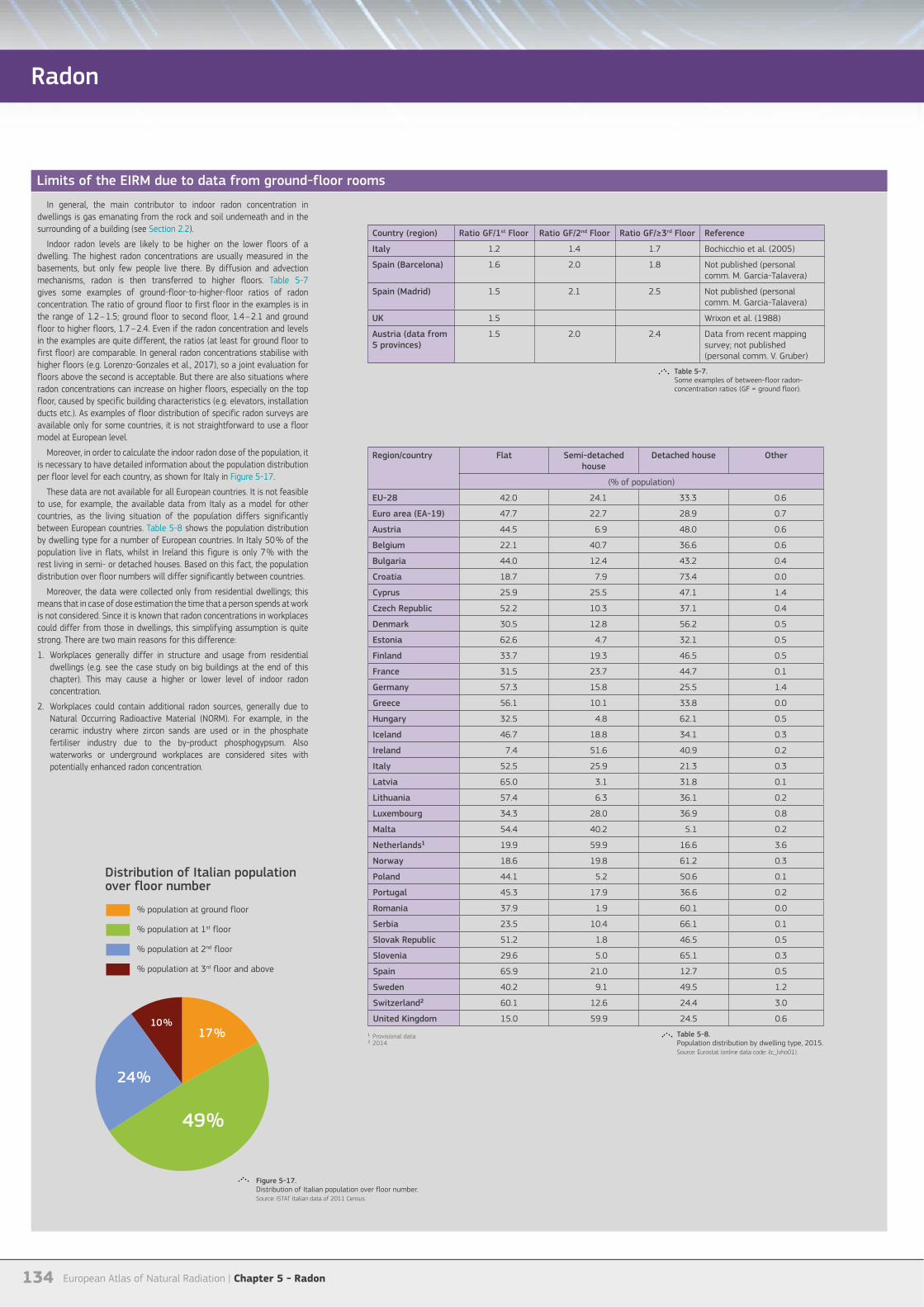
European Atlas of Natural Radiation | Chapter 5 - Radon134
Radon
Limits of the EIRM due to data from ground-floor rooms
In general, the main contributor to indoor radon concentration in dwellings is gas emanating from the rock and soil underneath and in the surrounding of a building (see Section 2.2).
Indoor radon levels are likely to be higher on the lower floors of a dwelling. The highest radon concentrations are usually measured in the basements, but only few people live there. By diffusion and advection mechanisms, radon is then transferred to higher floors. Table 5-7 gives some examples of ground-floor-to-higher-floor ratios of radon concentration. The ratio of ground floor to first floor in the examples is in the range of 1.2 – 1.5; ground floor to second floor, 1.4 – 2.1 and ground floor to higher floors, 1.7 – 2.4. Even if the radon concentration and levels in the examples are quite different, the ratios (at least for ground floor to first floor) are comparable. In general radon concentrations stabilise with higher floors (e.g. Lorenzo-Gonzales et al., 2017), so a joint evaluation for floors above the second is acceptable. But there are also situations where radon concentrations can increase on higher floors, especially on the top floor, caused by specific building characteristics (e.g. elevators, installation ducts etc.). As examples of floor distribution of specific radon surveys are available only for some countries, it is not straightforward to use a floor model at European level.
Moreover, in order to calculate the indoor radon dose of the population, it is necessary to have detailed information about the population distribution per floor level for each country, as shown for Italy in Figure 5-17.
These data are not available for all European countries. It is not feasible to use, for example, the available data from Italy as a model for other countries, as the living situation of the population differs significantly between European countries. Table 5-8 shows the population distribution by dwelling type for a number of European countries. In Italy 50 % of the population live in flats, whilst in Ireland this figure is only 7 % with the rest living in semi- or detached houses. Based on this fact, the population distribution over floor numbers will differ significantly between countries.
Moreover, the data were collected only from residential dwellings; this means that in case of dose estimation the time that a person spends at work is not considered. Since it is known that radon concentrations in workplaces could differ from those in dwellings, this simplifying assumption is quite strong. There are two main reasons for this difference:
1. Workplaces generally differ in structure and usage from residential dwellings (e.g. see the case study on big buildings at the end of this chapter). This may cause a higher or lower level of indoor radon concentration.
2. Workplaces could contain additional radon sources, generally due to Natural Occurring Radioactive Material (NORM). For example, in the ceramic industry where zircon sands are used or in the phosphate fertiliser industry due to the by-product phosphogypsum. Also waterworks or underground workplaces are considered sites with potentially enhanced radon concentration.
% population at ground floor
% population at 1st floor
% population at 2nd floor
% population at 3rd floor and above
Distribution of Italian population over floor number
49 %
17 %10 %
24 %
Region/country Flat Semi-detached house
Detached house Other
(% of population)
EU-28 42.0 24.1 33.3 0.6
Euro area (EA-19) 47.7 22.7 28.9 0.7
Austria 44.5 6.9 48.0 0.6
Belgium 22.1 40.7 36.6 0.6
Bulgaria 44.0 12.4 43.2 0.4
Croatia 18.7 7.9 73.4 0.0
Cyprus 25.9 25.5 47.1 1.4
Czech Republic 52.2 10.3 37.1 0.4
Denmark 30.5 12.8 56.2 0.5
Estonia 62.6 4.7 32.1 0.5
Finland 33.7 19.3 46.5 0.5
France 31.5 23.7 44.7 0.1
Germany 57.3 15.8 25.5 1.4
Greece 56.1 10.1 33.8 0.0
Hungary 32.5 4.8 62.1 0.5
Iceland 46.7 18.8 34.1 0.3
Ireland 7.4 51.6 40.9 0.2
Italy 52.5 25.9 21.3 0.3
Latvia 65.0 3.1 31.8 0.1
Lithuania 57.4 6.3 36.1 0.2
Luxembourg 34.3 28.0 36.9 0.8
Malta 54.4 40.2 5.1 0.2
Netherlands¹ 19.9 59.9 16.6 3.6
Norway 18.6 19.8 61.2 0.3
Poland 44.1 5.2 50.6 0.1
Portugal 45.3 17.9 36.6 0.2
Romania 37.9 1.9 60.1 0.0
Serbia 23.5 10.4 66.1 0.1
Slovak Republic 51.2 1.8 46.5 0.5
Slovenia 29.6 5.0 65.1 0.3
Spain 65.9 21.0 12.7 0.5
Sweden 40.2 9.1 49.5 1.2
Switzerland² 60.1 12.6 24.4 3.0
United Kingdom 15.0 59.9 24.5 0.6
¹ Provisional data² 2014
Country (region) Ratio GF/1st Floor Ratio GF/2nd Floor Ratio GF/≥3rd Floor Reference
Italy 1.2 1.4 1.7 Bochicchio et al. (2005)
Spain (Barcelona) 1.6 2.0 1.8 Not published (personal comm. M. Garcia-Talavera)
Spain (Madrid) 1.5 2.1 2.5 Not published (personal comm. M. Garcia-Talavera)
UK 1.5 Wrixon et al. (1988)
Austria (data from 5 provinces)
1.5 2.0 2.4 Data from recent mapping survey; not published (personal comm. V. Gruber)
Table 5-8.Population distribution by dwelling type, 2015.Source: Eurostat (online data code: ilc_lvho01).
Table 5-7.Some examples of between-floor radon-concentration ratios (GF = ground floor).
Figure 5-17.Distribution of Italian population over floor number.Source: ISTAT Italian data of 2011 Census.

Chapter 5 - Radon | European Atlas of Natural Radiation 135
attachment to aerosol
detachmentby recoil 0.1 – 1 µm
decay
exhalationfrom building
material air exchange
infiltrationfrom ground
cluster,(+) charged and uncharged,~ 1 nm
indoor
radon gas progeny
outdoor
depositionon surfaces(plate-out)can beused forretropectivedosimetry
risk factorssmoking, age, sex
relationdepends
on variousvariablefactors
risk:lung cancerprobability,incidence
dose(mSv)
atmosphere:equilibrium factor,
unattached fraction individual:breathing rate,smoking, age
radiology→doseconversion factor
physiology
epidemiology
exposure toRn progeny
(Bq*h/m3, WLM)
Environmental pollutant:
Rn concentrationin air (Bq/m3)
5.4.4 How can the dose due to radon be estimated?
The main hazard due to radon is caused by its short-lived alpha-emitting progeny (see details in Section 2.2.1). The damage which they inflict on the bronchial tissue depends on the size distribution of the radon progeny bearing clusters and aerosols that are in close contact with the tissue (UNSCEAR, 2008).
The relevant 222Rn progeny are 218Po (with a half-life of 3.05 min and relevant alpha energy of 6.0 MeV) and 214Po (164 µs; 7.7 MeV) for the 238U decay series and 216Po (145 ms; 6.8 MeV) and 212Po (0.3 µs; 8.8 MeV) for the 232Th series (progeny of 220Rn, also called thoron). Radon gas itself does not stick to lung tissue and has mostly been exhaled before it decays. This is somewhat different for 222Rn and 220Rn. Due to its short half-life, the latter has a higher probability of decaying while in the lung, i.e. before being exhaled, than the former. However, radon gas is soluble in tissue and contributes in this way to exposure and dose, but less than its decay products. In comparison, 222Rn and 220Rn have alpha energies of 5.5 and 6.3 MeV, respectively. To compare further, the parent nuclides 238U, 226Ra and 232Th have alpha energies of 4.2, 4.8 and 4.0 MeV, the terrestrial natural nuclides 147Sm and 144Nd have 2.2 and 1.8 MeV, and the artificial radionuclides 239Pu and 241Am have 5.2 and 5.5 MeV (all data from the Lund catalogue; Chu et al., 1999). The high alpha energies of some of the 222Rn and 220Rn progeny, together with their capability to irradiate the lung tissue attached to small aggregates, explain their high radiological efficiency.
Radon progeny produced by radon entry indoors reacts very fast with trace gases and air vapours of the indoor air and becomes small aerosol particles with diameters of 0.5 - 5 nm, called clusters or 'unattached' radionuclides. Besides forming clusters, radon progenies attach to the existing aerosol particles with diameters of 10 - 1 000 nm, called 'attached' radionuclides (see Section 2.2.2 for more details and references, Figure 5-18). The aerosol particles, which now carry the radon progeny, diffuse in the indoor atmosphere and deposit on any available room surface. The most hazardous aggregation mode is the ultrafine one, consisting of clusters of progeny atoms. The ratio of progeny activity concentration contained in this part, to total progeny concentration, called unattached fraction, f, as well as the equilibrium factor, F, are therefore relevant parameters in radon dosimetry (see Section 2.2.1 and above).
There are different ways to quantify the health hazard: • the organ dose to the lung generated by a given exposure to Rn
or Tn progeny (dosimetric approach);
• the effective dose;
• the effective dose corresponding to exposure to a certain activity concentration of 222Rn or 220Rn;
• the health detriment caused by exposure (epidemiological approach).
Dose calculationThe following formula can be used to estimate the effective
dose due to radon exposure:
RP
C = A . e . ß . (1 - p) p-1
C∞
(-log10(k) - 10)=
F ARa D0
0.75
. ρb .
.
λ p exp(-6 Sp - 6S14p)
D0 exp(-6 Sp - 6S14p)
J2
(m + λ222 . Co) . V
S
. ε .
. ε .
T273( )= √
(
[ ]( )
)
FTn ARa-224 ρb λTn
. e-λt . (1 - e-λt )
(C - C0e-λt )
S(1 - e-λt )
+
=
E222=
E0=
NRL=
δA δa12 + δa2
2 + δa32 + .. . + δan
2
2(Measured Mean - Reference Value
Reference Value
=
D
WL = EEC (Bq /m3)/3 700 = F *CRn (Bq /m3)/3 700
PAEE(WLM) = PAEC(WL) *
DC * EEC * t DC * F * t * CRn=
% PME × 100 +=
=
λ 220 . V0
-λ . (V / Q)220 1S
Cm
eE220
E222
=
λ . V
λ . V
1 - Φ 12 σ2x
1 - eln (Ri - R0) - µ
σ
( )Exposure (h)170
[ ]( )2
Standard Deviation
Measured Mean× 100
Ct C0=
√
√
√
-(x-µ)2
2σ2 -(x-µ)2
2σ2-∞
i 0ln (R - R )
∫
(5-1)
(5-2)
(5-4)
(5-5)
(5-7)
(5-8)
(5-9)
(5-6)
(5-10)
(5-11)
(5-12)
(5-13)
(5-14)
(5-3)√
√
NAPL Pi =−J ± −4CH
2H
π
where:DC is the dose coefficient (in general Sv or Gy per BqEEC hm-3);EEC=CRn * F is the Equivalent Equilibrium Concentration (EEC) of radon daughters;t is the exposure time;CRn is the radon concentration in Bq/m3;F is the equilibrium factor.
The parameters used in Equation 5-12 could be chosen according to some hypotheses that will be described in detail below.
Dose coefficient One of the key parameters in Equation 5-12 is the Dose
Coefficient (DC). This is a tool for converting an exposure quantity into a dose quantity. Radon exposure can be expressed in working level months (WLM), as a cumulative alpha energy concentration in mJ·h·m-3, or as a cumulative 222Rn activity concentration in MBq·h·m-3.
Historically, there have been many attempts to define the most appropriate DCs. Two different approaches have been explored: the epidemiological approach and the dosimetric approach (see Figure 5-19). In the epidemiological approach, essentially, the
measured radon concentration is compared with observed lung cancer incidence or mortality. In the dosimetric approach, the causal physical chain from concentration over exposure to dose and finally to risk is modelled, based on data on atmospheric processes, properties of persons, physiology of the lung, and knowledge about biological radiation effects. Only recently could a good correspondence between the results of the two approaches be achieved (ICRP Publication 137; ICRP, 2017). Both approaches are complicated in their details and involve many sources of uncertainty.
The epidemiological approach is based on epidemiology studies that consist of investigating connections between lung cancer cases and radon exposures. These studies consider large numbers of case-control data, and thus they produce a factor that converts radon concentration into doses. Three main epidemiological studies have been performed respectively in Europe (Darby et al., 2005, 2006), in the US (Kremski et al., 2006) and in China (Lubin et al., 2004). In 2016, Seungsoo et al. (2016) published a review of case-control studies in the world and concluded that the risk factors attributed to lung cancer were almost the same as the classical pooling studies.
The dosimetry approach considers mathematical models to evaluate the dose to the lungs due to inhalation of radon gas and its daughters. An analysis of information on aerosol size distribution, unattached fraction, breathing rate, fractional deposition in the airways, mucous clearance rate, and location of the target cells in the airways should be considered. Such estimates are model-dependent and necessarily subject to all
of the uncertainties associated with the input data as well as the assumptions built into the particular calculation model. The dosimetric evaluation of the absorbed dose to basal cells of the bronchial epithelium per unit exposure gives values in the range of 5-25 nGy (Bq EEC h m-3)-1 (UNSCEAR, 2000). The central value has been estimated by UNSCEAR to be 9 nGy (Bq EEC h m-3)-1 for average indoor conditions, a breathing rate of 0.6 m3 /h, an aerosol median diameter of 100 - 150 nm and an unattached fraction of 0.05.
EIRM and exposureAgain it should be emphasised that the cell mean (AM or median over
cell means) is an estimate of the spatial mean of the quantity 'long-term mean radon concentration in ground-floor rooms of dwellings', but neither (a) the mean over radon in ground-floor dwellings, nor (b) the mean over all dwellings, i.e. an estimate of exposure. For (a) one would have to calculate a weighted mean with population density at ground floor by cells as weights; and for (b) the distribution of dwellings over floors would have to be included as weight, together with a model which accounts for floor level. Demographically-weighted mean radon concentrations and mean exposure are generally lower than the spatial mean of the quantity discussed here, since:
• population centres are preferentially located in valleys and flatlands, in many cases over quaternary geology which usually has lower radon potential; and
• radon concentration decreases with floor level, on the average (see Section 5.4.3, coloured box).
Figure 5-18.Simplification of the radon progenies behaviour in indoor air and attachment to aerosol particle (details in Figure 2.11, Section 2.2.1).Source: Graph created by Peter Bossew.
Figure 5-19.Epidemiological and dosimetric approaches to assess radon risk.Source: Graph created by Peter Bossew.

European Atlas of Natural Radiation | Chapter 5 - Radon136
Approach Workers(mSv/WLM)
Members of Public
(mSv/WLM)
ICRP Publication 65 (1993)
Epidemiological 5 4
ICRP Publication 137 (2017)
Dosimetric 10 10
ICRP Publication 137 (2017)
Dosimetric 20*
Marsh & Birchall (2000) HRTM
Dosimetric 15
UNSCEAR (2006) Average value 5.7
Radon
Several ICRP publications by ICRP over the last years have proposed different DCs. ICRP Publication 65 (ICRP, 1993) suggested using a factor of 5 mSv per WLM for workplaces and 4 mSv per WLM for homes. Published in 1993, this document was widely accepted in the community. Updated versions were published in 2007 and 2010 (ICRP Publications 103 and 115, respectively). The last one in this series is ICRP Publication 137 (ICRP, 2017). This is an interesting document since it shows a good agreement between the latest dosimetric studies and the epidemiological approach.
Exposure timeExposure time (t) can be estimated by considering an
occupancy fraction of 0.8 (UNSCEAR, 2008). The occupancy fraction is the proportion of time that a person spends indoors.
For dose calculations, the exposure time per year is generally set to 7 000 h per year (~365 d/a × 24 h/d × 0.8).
However, differences could appear between European countries due to climate and living habits. Future versions of this Atlas may include further research on this topic.
Equilibrium factor The equilibrium factor F is defined as the ratio of the EEC (the
radon concentration in equilibrium with its decay products that equals the potential alpha-energy concentration of the original mixture) to the radon concentration.
Based on the currently limited available F measurements, UNSCEAR (2000-2008) provides a typical value of 0.4 for indoor radon in dwellings. F increases with increasing BqEEC/m3 aerosol particle concentration. It is thus affected by factors such as presence of tobacco smoke (Jasaitis & Grigzdy, 2013) and ventilation. For German dwellings Wicke and Postendörfer (1981) reported a range of F values from 0.3 to 0.6, for normal ventilation rates (0.1 – 1 h-1). More details are provided in Section 2.2.2.
Regional variations have been observed. For Sweden a mean value of 0.44 has been obtained (Swedjemark, 1983). In Canada, long-term measurements of F gave results ranging from 0.6 to almost 1 (Harley, 2018). Measurements carried out from different studies over the years in Chinese dwellings gave an average of 0.47, whereas in India a typical value of 0.36 has been proposed (Chen & Harley, 2018). In general, warm, humid areas seem to present lower F values.
* For the specific situations of indoor work involving substantial physical activity, and exposures in tourist caves (ICRP Publication 137, 2017)
Terminology
Working Level (WL)
Exercise on dose coefficients' influence
When speaking about 'radon', sometimes one means 222Rn and 220Rn indiscriminately. However, more often it denotes 222Rn only. 220Rn is often called thoron (Tn).
To make it more confusing, if speaking about 'radon exposure' or 'exposure to radon', one means exposure to radon progeny, in most cases. Again, distinction between 222Rn and 220Rn (=Tn) progeny is often not made.
We recommend using exact terminology to avoid any misunderstanding. Only when addressing the hazard caused by the Rn isotopes and their progeny in a generic way may one speak about 'radon'.
Another important unit when working with radon is the Working Level (WL). This unit was originally used for uranium mines, but it can be used on environmental exposures as well. A WL is any combination of short-lived radon daughters in one litre of air that will result in the emission of 1.3 × 10⁵ MeV of potential alpha energy (20.8 μJ/m3).
The equivalences for expressing potential alpha-energy concentration (PAEC) in relation to equilibrium equivalent concentration (EEC) are:
• PAEC of 1 J/m3 corresponds to 1.8 × 10⁸ BqEEC/m3
• PAEC of 1 WL corresponds to 3.75 × 10³ BqEEC/m3 and correspondingly
the potential alpha energy exposure (PAEE)
• PAEE of 1 J h m-3 corresponds to 1.8 × 10⁸ BqEEC h/m3 and
• PAEE of 1 WLM corresponds to 6.37 × 10⁵ BqEEC h/m3.
In this way, one WL is roughly 3 700 Bq/m3 equilibrium equivalent concentration of radon (EEC):
RP
C = A . e . ß . (1 - p) p-1
C∞
(-log10(k) - 10)=
F ARa D0
0.75
. ρb .
.
λ p exp(-6 Sp - 6S14p)
D0 exp(-6 Sp - 6S14p)
J2
(m + λ222 . Co) . V
S
. ε .
. ε .
T273( )= √
(
[ ]( )
)
FTn ARa-224 ρb λTn
. e-λt . (1 - e-λt )
(C - C0e-λt )
S(1 - e-λt )
+
=
E222=
E0=
NRL=
δA δa12 + δa2
2 + δa32 + .. . + δan
2
2(Measured Mean - Reference Value
Reference Value
=
D
WL = EEC (Bq /m3)/3 700 = F *CRn (Bq /m3)/3 700
PAEE(WLM) = PAEC(WL) *
DC * EEC * t DC * F * t * CRn=
% PME × 100 +=
=
λ 220 . V0
-λ . (V / Q)220 1S
Cm
eE220
E222
=
λ . V
λ . V
1 - Φ 12 σ2x
1 - eln (Ri - R0) - µ
σ
( )Exposure (h)170
[ ]( )2
Standard Deviation
Measured Mean× 100
Ct C0=
√
√
√
-(x-µ)2
2σ2 -(x-µ)2
2σ2-∞
i 0ln (R - R )
∫
(5-1)
(5-2)
(5-4)
(5-5)
(5-7)
(5-8)
(5-9)
(5-6)
(5-10)
(5-11)
(5-12)
(5-13)
(5-14)
(5-3)√
√
NAPL Pi =−J ± −4CH
2H
π
Traditionally, the exposure of uranium miners and other mine workers has been expressed in units of Working Level Month (WLM). This is the exposure rate of 1 WL for a working month of 170 hours. Thus, while a miner exposed to 1 WL during a working year accumulates 12 WLM, a member of the population with continuous exposure to 1 WL accumulates about 50 WLM. In that way,
RP
C = A . e . ß . (1 - p) p-1
C∞
(-log10(k) - 10)=
F ARa D0
0.75
. ρb .
.
λ p exp(-6 Sp - 6S14p)
D0 exp(-6 Sp - 6S14p)
J2
(m + λ222 . Co) . V
S
. ε .
. ε .
T273( )= √
(
[ ]( )
)
FTn ARa-224 ρb λTn
. e-λt . (1 - e-λt )
(C - C0e-λt )
S(1 - e-λt )
+
=
E222=
E0=
NRL=
δA δa12 + δa2
2 + δa32 + .. . + δan
2
2(Measured Mean - Reference Value
Reference Value
=
D
WL = EEC (Bq /m3)/3 700 = F *CRn (Bq /m3)/3 700
PAEE(WLM) = PAEC(WL) *
DC * EEC * t DC * F * t * CRn=
% PME × 100 +=
=
λ 220 . V0
-λ . (V / Q)220 1S
Cm
eE220
E222
=
λ . V
λ . V
1 - Φ 12 σ2x
1 - eln (Ri - R0) - µ
σ
( )Exposure (h)170
[ ]( )2
Standard Deviation
Measured Mean× 100
Ct C0=
√
√
√
-(x-µ)2
2σ2 -(x-µ)2
2σ2-∞
i 0ln (R - R )
∫
(5-1)
(5-2)
(5-4)
(5-5)
(5-7)
(5-8)
(5-9)
(5-6)
(5-10)
(5-11)
(5-12)
(5-13)
(5-14)
(5-3)√
√
NAPL Pi =−J ± −4CH
2H
π
Figure 5-20 shows how the annual effective dose due to radon exposure depends on the values chosen for the dose coefficient. The following parameter values have been assumed to estimate the dose:
• 100 Bq/m3 Rn concentration at home;
• 0.8 as occupational factor;
• 0.4 as equilibrium factor.
ICRP 65 (1993)0
1
2
3
4
5
6
7
mSv
8
Marsch& Birchall (2000)
Annual effective dose
UNSCEAR (2006) ICRP 137 (2017)
Table 5-9.Dose coefficients based on different models in mSv/WLM.Source: Table created by Marta García-Talavera and José-Luis Gutiérrez Villanueva.
Figure 5-20.Comparison of the annual effective doses due to radon exposure estimated using different dose coefficients.Source: EANR, EC-JRC, 2019.
Small, former uranium mines, Urgeiriça, Central-Eastern Portugal, close to the Spanish border.Source: Peter Bossew.

Chapter 5 - Radon | European Atlas of Natural Radiation 137
0 100 200 300 400 500 600 700
Floor Building D1
Radon concentration (Bq/m3)
0
1
2
3
4
5
6
7
8
9
10
11
12
13
14
15
100 200 300 400
Lognormal distribution
500 600 700 800
Empirical distribution
Rn [Bq/m3]
Freq
uenc
y
20
15
10
5
0
Case study: Radon measurements in large buildingsThe European Basic Safety Standards Directive (European
Union, 2013) includes regulations of radon in common workplaces and public buildings for the first time in radioprotection regulation. The EU Member States must transpose this Directive into national law, and even some non-Member States, although not obliged, chose to adopt regulations which closely follow it. A number of questions arose concerning the practical application of these new standards, such as how to perform representative, reproducible and legally compliant measurements of radon concentration in large buildings. As a basis for deciding further action, as laid down in the Radon Action Plans (also an obligatory part of the Basic Safety Standards Directive (European Union, 2013) transposition), measured values have to be compared with a defined reference level (RL). The BSS stipulates that EU Member States must set an RL of maximum 300 Bq/m3. The RL is valid not only for residential indoor radon, but also for workplaces and for public buildings.
In the past years, the mechanism of radon infiltration and accumulation in private dwellings has been investigated, understood and resolved in many cases. Only a few investigations have been performed in 'large' buildings such as administration edifices, schools, factories, supermarkets or business centres (Jeong et al., 2013). As one can imagine, these constructions are in general much more complex and their 'users' behave quite differently and with greater diversity (for example concerning air exchange, which is the key anthropogenic parameter that controls indoor radon concentration, together with the geogenic radon potential) than in residential buildings.
The international Radon in Big Buildings (Ribibui) Consortium (http://www.ribibui.org), established in February 2016 at the University of Applied Sciences and Arts (SUPSI) in Lugano, Switzerland, is investigating strategies to define a standard protocol for radon measurements in these objects. To this end, radon measurement data from 'large' buildings in various countries have been collected and analysed so far. As one can anticipate, the radon characteristics differ between types of 'large' buildings, and, consequently, a tentative classification of building types has been proposed by the consortium (see Table 5-10). Understanding the differences between building classes is a prerequisite for modelling the radon distribution and its migration pathways.
For logistic and economic reasons, only in a few cases is it possible to place radon detectors everywhere in a large building with a large number of rooms. Therefore, an important result of the project will be to propose an estimate of how many detectors are necessary within a large building, and where they have to be located, in order to be able to decide with given confidence whether further action (e.g. remediation) according to the Radon Action Plan is necessary or not. In most cases, this is a decision about compliance with the RL. Developing a method for such decision, and assessing its reliability (or the factors which determine it), is one of the objectives of this project.
To date, the majority of large buildings for radon concentration are schools, kindergartens and office buildings. In most cases, basement, ground- and first-floor rooms have been measured, but rarely rooms on higher floors because most of these measurements were performed outside the project environment. Based on experiences in dwellings, it has been assumed that also in workplace-type buildings a decrease of radon concentration with increasing floor level is the rule. Reflecting the state of knowledge around 2010, when it was developed, also the Basic Safety Standards Directive requires measurements in workplaces (when it is required at all, namely in radon priority areas) only in basement and ground floor rooms. However, the first results of the Big Buildings project have shown that in certain types of buildings one cannot rely on that rule. In fact, some measurement data show higher radon concentration on upper floors (see Figure 5-21 as an example), which might be caused by lower pressure differences between indoor/outdoor atmosphere and consequently of less natural air exchange. It is known that artificial ventilation or air conditioning systems influence the radon distribution (Kozak et al., 2014; Polednik et al., 2016). These kinds of effects have to be considered in a standard protocol. An example of the distribution of radon concentration in a building is shown in Figure 5-22, for a building without significant dependence of radon on floor level. If there is a dependence, in particular the one mostly observed in lower residential buildings, the overall frequency distribution should be assumed multimodal, reflecting distinct modes of radon entry in different compartments (floors) of the building.
Quantities for characterising the radon situation of a building could be, among others, the mean radon concentration over all rooms or the probability that any room has radon concentration levels above the RL. Finding the values of these quantities, as a basis for deciding about compliance with regulation, requires performing radon measurements, perhaps together with additional assumptions about radon distribution. A more profound understanding and analysis is required and will be performed in the near future.
Type number Building description
1 Mall or manufacturing type (large halls, large commercial centres) [nfloors < 3]
2 Flat hall type (schools, kindergartens) [nfloors <= 3]
3 Standard office type [3 < nfloors < 10]
4 Skyscraper type [nfloors > 9]
5 Sport stadium type
6 Historical buildings
7 Underground workplaces
8 Other
Figure 5-21.Measured radon concentration in a building with 15 floors (floor 14 not measured). Each box ranges between the 25th and 75th percentiles, the crosses represent the mean, the black horizontal lines the median, the lines extending vertically from the boxes (whiskers) indicate variability outside the upper and lower quartiles and the points represent the outliers.Source: Graph created by Marcus Hoffmann.
Figure 5-22.Radon concentration distribution in a building with 15 floors, fitted with a Lognormal distribution (AM = 251, GM=228, GSD=1.55) and the empirical distribution.Source: Graph created by Marcus Hoffmann.
Table 5-10.Building type classification by the Radon in Big Buildings project.Source: Marcus Hoffmann.


![Indoor Air Quality (IAQ) - Radon · Radon, please call your State Radon Contact or the National Radon Information Line at: 1-800-SOS-RADON [1 (800) 767-7236], or (if you have tested](https://static.fdocuments.in/doc/165x107/5fb2e8f6d1a5cc5c8d33d275/indoor-air-quality-iaq-radon-radon-please-call-your-state-radon-contact-or.jpg)