RADIOSCIENCE LABORATORY .QI

r= STANFORD ELECTRONICS LABORATORIESDEPARTMENT OF ELECTRICAL ENGINEERING

"STANFORD UNIVERSITY • STANFORD, CA 94305

m ULF/ELF ELECTROMAGNETIC FIELDS

I ' PRODUCED IN SEA WATER BY LINEARr CURRENT SOURCES

by

A.S. Inan•.C. Fraser-SmithO.G. Villard, Jr.

Technical Report E721-1

S�~uFebruary 1982

•"SEP 1. 1982

Sponsored byThe Office of Naval ResearchthroughContract No. N00014-79-C-0848

' t,¥

Reproductir.1j in whole or in part is permitted for any

purpose of the U. S. Government.

The views and conclusions contained in this document

are those of the authors and should not be inter-

preted as necessarily representing the official

policies, either expressed or implied, of the Office

of Naval Research or the U. S. Government.

PAGESARE

MISSING

INORIGINAL

DOCUMENT

UNCLASSIFIED- SECURITY CL.ASSIFICATION OF THIS PAGE [Wheln Oats Entitred)

REPORT DOCUMENTATION PAGE BFREA COMPLECTINFON M

1 REPORT NUMBER 2, GOVrT ACCESSION NO. 3. RECIPIENT*S CATALOG NUMBER

Technical Report No. E721-1l po-A 3L

ULF/ELF Electromagnetic Fields Produced in SeaTehia

Water by Linear Current So-irces 15 August 1979-31 January 1982

6. PERFORMING ORG. REPORT NUMWE--R

7A. s. man E721-1 O UBRI

A. S. Inan 8 CONTRACT ORGRANT NME11

A. C. Fraser-Smith N00014-79-C-08480. G. Villard, Jr.

9 PERFORMING ORGANIZATION NAME AND ADDRESS 10. PROGRAM ELEMENT, PROJECT, TASK

Radioscience Laboratory AREA & WORK UNIT NUMBERS

Stanford Electronics Lab., Stanford University Task Area NR 089-151Stanford, California 94305 12. REPORT DATE 1-i3. NO.0 OF PAGES

11 CONTROLLING OFFICE NAME AND ADDRESS 118ar 98Office of Naval Research, Code 414 15. SECURITY CLASS. (of this report)800 North Quincy StreetArlington, VA 22217 UNCLASSI FIED

14 MeoNiTC7RING AC.ENCY NAME & ADI)RESS (if dtf. fromn Conltrolling Officis)

115s. DECLASSIFICATION 'DOWNGRADINGSCHEDULE

¶ ~18. DISTRIBUJTION STATEMENT (0f this report)

Approved for public release; distribution unlimited.

17 DISTRIBUTION STATEMEriT (of th. abstract entered in Block 20, it diffoilrsot from report)

18 SUPPLEME.YTARY NOTES

19 KEY WORDS ICont,rit,, on re~sor* side if necesotsry *nd Identify by block numcier)UJNDERSEA COMMUNICATIONSUBMERGED CABLESULF/ELF"LEADE GEAR"POIjNT .LECTRODES

70 A~ AT I~nnr...on reverie side A necessary ise identify Ut' block numnber)__rThis r'eport is concerned with the possibility of using undersea cables tocommunicate with undersea receivers at frequencies in the L'lt-.d low and extremelylow ranges. Because of the low data transmission rate at these frequencies, comn-munication is here understood to mL~.;, the transfer of short messages of highInformation content.

We start by deriving theoretical expressions for the electric and magneticfields generated in conducting medium of infinite extent by linear current

FORMUCLSIFlE1D JAN 731 7 UNCLASSIFIED _______________

EDITION OF I NOV 65 IS OBSOLETE SECURITY CLASSIFICATION OF THIS FAGE fWhen Date Entered)

ji- I' r

UNCLASSI FIEDSECURITY CLASSIFICATION OF THIS PAGE (When Data CnteriadtSIL 19 KEN WORDS (Continued)

V1 APSTRACT ,Con,nnuea)

sources (i.e., straight insulated current-carrying cables) of finite andsemi-infinite length and of finite length with gaps of either finite or infini-ftesimal size., Next, using numerical integration techniques and, in some cases,a parametriiE. :"presentation to make our results frequency independent, we com-pute representative numerical values of the field amplitudes for the abovediscontinuous sources. For comparison with these data, we compute an extensiverange of field amplitudes for the more frequently encountered continuous linearsource of infinite length (i.e., a very-long straight insulated current-carryingcable); we also introduce a parametric representation for the fields produced bythis reference source and we show that for any fixed perpendicular distance fromthe source there is an optimum frequency for electric field generation.

We show that the discontinuous sources generally produce greatly enhancedelectric fields in the vicinity of their open ends, as compared with the con-tinuous source. However, at large distances none of the discontinuous sourceswe have considered produce larger fields than the continuous source, and inmost cases the discontinuous sources produce smaller fields. These resultssuggest that the optimum use of the discontinuous sources (short lengths ofcurrent-cari-ying cab.e; point electrodes) is for short-range undersea comrmunica-SI tion, whereas long continuous current-carrying cables appear to have the mostpromise for long-range communication via their electric and magnetic fields.

Finally, because even long cables have limited communication ranges at allbut the lowest ultra low frequencies, we consider the use of arrays of parallellong cables to produce measurable electric and magnetic fields throughoutspecific regions of the sea. Our data indicate, for example, that a seriesconnected array of 10 long cables (each of length L) laid on the floor of a sea1 km deep and carrying a 1000 A, 1 Hz current could produce meas rable magneticfields throughout the sea over a horizontal area of about 75L km'. Such arrayscould find use in crucial areas where reliable undersea communication is of highpriori ty.

FOR JN314 (BArK _________ _____DD1 JAN 7314JrO UNCLASSIFIEDEDITION OF 1 NOV 65 IS OBSOLETE SECURITY CLASSIFICATION OF THIS PAGE iWhen Oata EnveeO)

ULF/ELF ELECTROMAGNETIC FIELDS PRODUCED IN

SEA WATER BY LINEAR CURRENT SOURCES

by

A. S. Inan

A. C. Fraser-Smith

0. G. Villard, Jr.

A c c e • .-.I o n F o r _• _ _

Technical Report E721-1 D 'J - ,Ell

................................ .... .. ...

"-D lftri'u'iu""'-li/

February 1982 1•.v , l- •I' v (Ins

Dist $pc ta1

Sponsored by

The Office of Naval Research / ,

through

Contract No. N00014-79-C-0848

AL .! ! ,7

ABSTRACT

This report is concerned with the possibility of using undersea

cables to communicate with undersea receivers at frequencies in the

ultra low and extremely low ranges. Because of the low data trans-

mission rate at these frequencies, communication is here understood to

mean the transfer of short messages of high information content.

We start by deriving theoretical expressions for the electric and

magnetic fields generated in a conducting medium of infinite extent by

linear current sources (i.t., straight insulated current-carrying

cables) of finite and semi-infinite length and of infinite length with

gaps of either finite or infinitesimal size. Next, using numerical

integration techniques and, in some cases, a parametric representation

to make our results frequency independent, we compute representative

numerical values of the field amplitudes for the above discontin'ous

sources. For comparison with these data, we compute an extensive range

of field amplitudes for the more frequently encountered continuous

linear source cf infinite length (i.e., a very-long straight insulated

current-carrying cable); we also introduce a parametric representation

for the fields produced by this reference source and we show that for

any fixed perpendicular distance from the source there is an optimum

frequency for electric field generation.

We show that the discontinuous sources generally produce greatly

enhanced electric fields in the vicinity of their open ends, as com-

pared with the continuous source. However, at large distances none of

the discontinuous sources we have considered produce larger fields

iii

t/

than the continuous sou;--e, and in most cases the discontinuous sources

produce smaller fields. These results suggest that the optimum use of

the discontinuous sources (short lengths of current-carrying cable;

point electrodes) is for short-range undersea commurnication, whereas

long continuous current-carrying cables appear to have the most promise

for long-range communication via their electric and magnetic fields.

Finally, because even long cables have limited communication

ranges at all but the lowest ultra low frequencies, we consider the use

of arrays of parallel long cables to produce measurable electric and

magnetic fields throughout specific regions of the sea. Our data

indicate, for- example, that a series connected array of 10 long cables

(each of length L) laid on the floor of a sea 1 km deep and carrying a

1000 A, 1 Hz current could produce measurable magnetic fields throughout.

2the sea over a horizontal area of about 75L km . Such arrays could find

use in crucial areas where reliable undersea communication is of high

priority.

iv

ACKNOWLEDGEMENT

Support for this work was provided by the Office of Naval

Research through Contract No. N00014-79-C-08 4 8 .

v

Note: In this report we use the abbreviation ULF (ultra-low-

frequencies) for frequencies less than 5 Hz, and we use

ELF (extremely-low-frequencies) to designate frequencies

in the range 5 Hz to 3 kHz.

i

vi

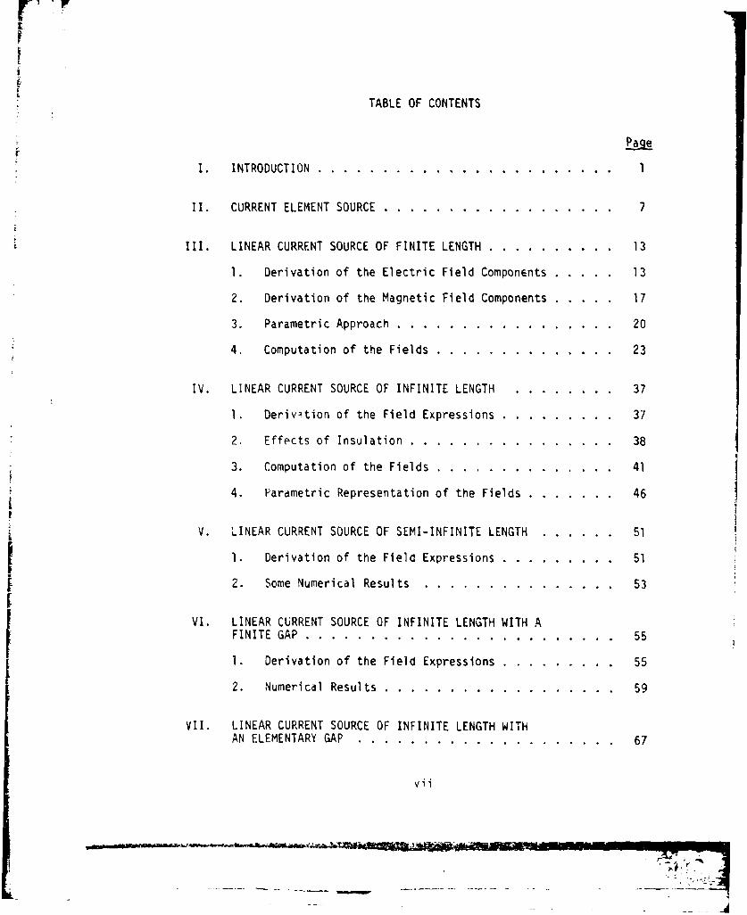
TABLE OF CONTENTS

I. INTRODUCTION ......... ....................... .....

II. CURRENT ELEMENT SOURCE ........... .................. 7

III. LINEAR CURRENT SOURCE OF FINITE LENGTH ...... .......... 13

1. Derivation of the Electric Field Components ........ 13

2. Derivation of the Magnetic Field Components ........ 17

3. Parametric Approach ...... ................. ... 20

4. Computation of the Fields ..... .............. ... 23

IV. LINEAR CURRENT SOURCE OF INFINITE LENGTH ..... ........ 37

1. Derivation of the Field Expressions ... ......... ... 37

2. Effects of Insulation ...... ................ ... 38

3. Computation of the Fields ..... .............. ... 41

4. Parametric Representation of the Fields ......... ... 46

V. LINEAR CURRENT SOURCE OF SEMI-INFINITE LENGTH .... ...... 51

1. Derivation of the Field Expressions ..... ......... 512. Some Numerical Results ..... ..... ............... 53

VI. LINEAR CURRENT SOURCE OF INFINITE LENGTH WITH AFINITE GAP ........... ... ........................ 55

1. Derivation of the Field Expressions ... ......... ... 55

2. Numerical Results ....... .................. ... 59

VII. LINEAR CURRENT SOURCE OF INFINITE LENGTH WITHAN ELEMENTARY GAP ..... ......... .................... 67

vii

-- IN

J-I

Page

VIII. SUMMARY AND CONCLUSIONS ....... ................. ... 69

1. Summary .......... ..... ....................... 69

2. Discussion ....... ..................... .... 71

3. Suggestions for Further Work ....... ............. 76

IX. REFERENCES ......... ..... ........................ 79

APPENDIX A. THE INFINITELY-THIN LINEAR CURRENT SOURCEAPPROXIMATION ....... ................... ... 83

APPENDIX B. INTRODUCTION TO THE KELVIN FUNCTIONS ......... ... 87

APPENDIX C. FIELDS PRODUCED BY A DC CURRENT ...... .......... 91

APPENDIX D. FIELDS PRODUCED BY ARRAYS OF LONG CABLES SUBMERGEDIN A CONDUCTIVE MEDIUM OF INFINITE EXTENT ........ 97

viii

I, INTRODUCTION

Shortly after the end of the First World War a pair of articles

appeared in the scientific literature describing experiments and theo-

retical work on the electromagnetic fields produced in, on, and above

the sea by submerged cables carrying alternating current [Drysdale,

1924; Butterworth, 1924]. As described in the article by Drysdale

[19241, and in greater detail in a later article b) Wright [1953], this

work was undertaken as part of a British Navy project called "Leader

Gear", which was concerned with the usE of the cable-generated electro-

magnetic fields for navigation. No further articles appeared on the

fields produced by submerged cables until after the end of the Second

World War, when Von Aulock prepared two lengthy unpublished reports on

the subject [Von Aulock, 1948, 1953]. With the exception of a useful

summary of Von Aulock's results by Kraichman [1976] and several particu-

larly pertinent articles by Wait [1952, 1959, 1960], little research

has since been carried out on the electromagnetic fields produced by

submerged cables. This is unfortunate, because it is our belief that

the fields could have important applications in undersea communication.

The primary objective of this report is to take the work just described

through a further stage uf development and thus provide an improved

theoretical basis for studies of the feasibility of the use of the

fields from submerged cables for undersea communication.

To achieve this objective, we start with the comparatively well-

known expressions for th(: electromagnetic fields produced in a conduct-

ing medium of infinite extent by a current element and then, always

S. .. .

,,,,

considering a conducting medium of infinite extent, to systematically

derive the other known expressions for (1) the electric field produced

by a linear current sou,ce of finite extent (i.e., by a short current-

carrying insulated wire or cable) and (2) the electric and magnetic

fields produced by a linear current source of infinite length (i.e., by

a long current-carrying insulated wire or cable). In passing we derive

(3) an expression for the magnetic field produced by the linear current

source of finite extent, which is a new result, and we solve this ex-

pression numerically to provide illustrative magnetic field data. We

then expand from this beginning by deriving (4) expressions for the

electric and magnetic fields produced by a linear current source of

semi-infinite extent, with particular emphasis on the fields produced

around the end of the source where the current enters the conducting

medium. These latter results are then used to give (5) expressions for

the electric and magnetic fields produced by two aligned, separated

semi-infinite linear current sources, i.e., the fields produced in the

vicinity of two point electrodes immersed in the conducting medium.

Finally, we allow the spacing between the ends of linear sources in (5)

to become infinitesimal and thus obtairn (6) expressions for the electric

and magnetic fields produced by a linear current source of infinite ex-

tent containing an infinitesimal gap. As we will show, these latter

expressir:,s can alsc be derived by subtracting the electric and magne-

tic field expressions for a current element from the equivalent expres-

sions fur a linear current source oF infinite length.

In cases (4) to \6) above we present representative numerical

2

values for the electric and magnetic fields that are produced. lie be-

lieve both these numerical values and the theoretical expressions for

the electromagnetic fields are new. We end with a brief discussion of

the possible application of the electric and magnetic fields to under-

sea communication.

There is one technical feature of our theoretical approach that

has general implications and which is best discussed at this introduc-

tory stage. It will be noted that we always assume an infinitely thin

cross-section for the various (cylindrical) linear currtnt sources con-

sidered in this work, whereas it is obvious that these sources will

have a finite cross-section in practice. Techni-ally, this assumption

takes the form of a replacement of a volume integral in the Hertz vec-

tor expression by an approximate line integral. The derivation of the

approximate line integral is given in Appendix A and it is shown that

the approximation is valid provided the shortest distance from the

observation point to the surface of the current source is much greater

than the radius of the source. Provided this condition is met, our

expressions should give accurate values for the electric and magnetic

fields produced by the linear current sources of finite cross-section.

The most important quantity to keep in mind in this work is the

skin depth 6 defined by

6 = (21w)v ½ (I.1)

for a magnetic (I , uo) conducting medium, where we use w for the angu-

00lar frequency, V1 for the permeability of the medium (V 0 is the permea-

bility of free space), and o for its conductivity. At the frequencies

3

eiaar ~ n..s. ~ a n a -~- ____________ -______-_

• 7#

considered in this report, electromagnetic fields propagate in a con-

ducting medium with a wavelength given by X 2 2 6, and evidence of this

wavelength will be seen in most of the figures showing numerical data.

In all cases these numerical data are computed for sea water, where we

assume a = 4.0 S/m and p = po = 4-, x 107 H/rn. Table 1.1 lists numeri-

cal values of skin depth for these assumed sea water parameters and for

frequencies in the range 0.001 - 1000 Hz.

The theory developed in this report assumes that the contribution

from the displacement current term in Maxwell's equations can be neg-

lected in comparison with the contribution from the conduction current

term. This is only possible for frequencies satisfying the condition

a/owc>>l , where c is the permittivity of the medium. In the case of

sea water, which is the conducting medium of primary inteest in this

work, the above condition implies that the frequencies must be very

much less than 890 MHz for our field expressiors to be valid. This

means that the frequencies must be below tte microwave range (the low-

est microwave frequency is usually taken to be 300 MHz) or, perhaps

more strictly, they must be less than 100 MHz. ,

For frequencies satisfying the condition /w l>>I (i.e., for fre-

quencies less than 100 MHz in sea water) it is easily shown th;,t elec-

tric fields propagating in a conductin, medium are attenuated at the

rate of 55 db/wavelength. This is a very substantial rate of attenua-

tion and it is obvious as a result that large ranges for communication

through sea water by means of electromagnetic signals can only be

achieved by using low frequencies. It is for this reason that we have

4

Table I.1 Representative Skin Depths for Sea Water

(as 4.0 S/m)

Frequency Skin Depth Frequency Skin Depth(Hz) (M) (Hz) (M)

1000 8.0 1 251.6

800 8.9 0.8 281.3

600 10.3 0.6 324.9

600 12.6 0.4 397.9

200 17.8 0.2 562.7

100 25.2 0.1 79E.8

80 28.1 0.08 889.7

60 32.5 0.06 1027.3

40 39.8 0.04 1258.2

20 56.3 0.02 1779.4

10 79.6 0.01 2516.5

8 89.0 0.008 2813.5

6 102.7 0.006 3248.7

4 125.8 0.004 3978.9

2 177.9 0.002 5627.0

1 251.6 0.001 7957.7

5

..-. .S_ . ._ . 8

Irestricted our computations of numerical data to frequencies in the-

extremely-low (ELF; frequencies in the range 5 Hz - 3 kHz) and ultra-

low (ULF; frequencies less than 5 Hz) frequency bands. At these low

frequencies the wavelength in sea water becomes usefully large (1.58 km

at 1 Hz) and reasonably large communication ranges become possible.

However, even at these low frequencies the same basic attenuation rate

of 55 ib/wavelength still applies and evidence for it will be found in

all cf our numerical data.

6

___7--W

II. CURRENT ELEMENT SOURCE

Suppose we have a homogeneous isotropic conducting medium of con-

Sductivity a, dielectric constant c, and permeability p. Assuming that

all the fields vary with time t as exp(iwt), MaxwelI's equations can

be written in the form

div E - 0 (11.1)

div H = 0 (11.2)

curl E =-iwPH (11.3)

curl H = (a + i W E)E + J (11.4)

where J is the impressed current density and where E and H are the elec-

tric and magnetic field intensities, respectively. We wish to obtain E

and H for a current element Idi immersed in this conducting medium,

which we will assume is of infinite extent.

In our derivation, and throughout this report, we will make exten-

sive use of the Hertz vector H [Panofsky and Phillips, 1962; Kraichman,

1976), from which the E and H fields can be obtained by using the follow-

ing equations in conjunction with Maxwell's equations II. - 11.4:

E = -y 2fl + grad div 11, (11.5)

2H = -Y-- curl H. (11.6)

Here, y, the propagation constant, is defined by

y = (itP ( + i C (11.7)

7

Substitution of Equations (11.5) and (11.6) into either (11.3) or

(II.4) yields the differential equation

2 _curl curl f - grad div U + y' = o+i (.

which can also be written as

2-j (_ 1.9)( Y723y2) WE: oIA)

This equation is called the inhomogeneous wave equation and for our un-

bounded conducting medium it has a solution of thE form (e.g., Wait,

1959)

A/ (e+iwc) I r J dv. (II.10)

V

For a current element source oriented in the z-direction in a

cylindrical coordinate system, as shown in Figure II.1, one can easily

verify that the Hertz vector at the point P has only a z-component given

by

R (P,Z) IdZ e I l

z 4Tr(aj+iWET rI.

where

8

-V.

r

9

Idt -- •,

ii

0

0, *4,,"" (p. @.o)

I

(0:O)

Figure 11.1. Coordinate system and geometry used in the derivation ofthe electric and magnetic fields produced in a conducting medium ofinfinite extent by a current element Idt.

9

r (2 + (zi)2)

Using this component of n, the electric and magnetic fields can be

obtained by performing the operations

a21

~ nz•= 0 , (11.12)

and

H 0P

-_ 2 z (11.13)

H =0

It follows from these equations that

E jjjnecosb ~2 2 eyrE0 'ineF3 (Y r +3-yr+3) e'4r(a+iwE• r

E =o , (1.14)

10

EZ• IdP 3 Cos [c52 e (Y2r 2 +3yr+3). (y 2 rZ yr+l e- r,4 t(+i we )r 3

and

P

H =0,Hý IdQ~sine -rl - (11.15)

4 TTr

Z 0

where sinO = J/r and cose = (z-z)/r.

These latter expressions completely describe the electromagnetic

fields produced in the medium by a current element scurce.

- -

S1 11

III. LINEAR CURRENT SOURCE OF FINITE LENGTH

Suppose now that we have an insulated thin straight wire extending

from ZI to Z2 on the z-axis of our coordinate system (Figure Il.1) and

carrying a cLrrent I exp(iwt), which we assume is constant throughout

the length of the wire. The surrounding conducting medium is again

assumed to be infinite and homogeneous with electric and magntLic pro-

perties ,3, E, and ui, as described in the previous section. We know that

for a highly conducting medium such as sea water (a = 4 S/m) it is rea-

sonable to neglect the displacement currents for all frequencies up to

the microwave frequency range. We can therefore replace (a+iiwc) by 0

in Equations (11.7) and (11.11), obtaining

,z(I,z) ldL e"-r

where, once again,

r (,2+(2,-_ ) 2 ½

II1.1 Derivation of the Electric Field Components

In this subsection we follow the approach used by Wait [1952] to

derive the components of the electric field produced by the finite

linear current source. We start with the expression for the Hertz vec-

tor produced by a current element IdZ (Equation 111.2). Integrating

13

from Z to k2, we obtain the Hertz vector for a finite linear current

source

5z (,z) _ l r2 I(Z)e -r dk (111.3)z 47T7 J r

Since we assumed that the current is constant throughout the wire,

the Hertz vector can be rewritten as

I e-Yr dz (III.4)11Z(p ,Z) = T' I

Substituting this in Equation (11.12), it follows that the p and z com-

ponents of the electric field are given by

(11J.5)

Ez - I P(r)dZ -I MO .r

Here the function P(r) and Q(r) are defined [Sunde, 1949; Wait, 1952]

as follows:

P(r) = i e-yr

e -yrQ r) (111.6)

14

-w --

". 1 "

2

PLi./.z

/ I

/

r r

-=

•

IP

Figure 1I1.1. Coordinate systeiw and geometry used in the oerivation ofthe electric ano wagnetic fields produced in a conducting medium ofinfinite extent by a linear current source of finite extent.

15

mi-m-

.. ,- ..

Making the following substitutions

S= l/ ( /2) , y (l+i),

x = 4ý zZ- , a . ,

u= (a 2 + x2 ) ½

the integral in Equation (111.5) can also be rewritten as

2 x2 (l+i)u

J P ( r ) d ; . - iu-..4 'J e d x ( 1 1 1. 7 )

where x1 = S(z--I) and x2= '(Z- 2 ) "i

This integral can be broken into three separate integrals:

x2) x2 x2 x1-2 2

-(l+i)u 1-e'Ucos u ex sin u

f dx f e cx s u - i dx.x1 x1 1 1

Here the second and third integrals are the ygnuralized cosine and sine

integrals, Ec [a,x] and E [a,x], which are defined as follows:

x

E[Cax] = .1 l-eUcos u dx ,

(111.8)X

e sin u dxEs[a'x] : o u

16

i ....

;'

Numerical values for these integrals are tabulated by Staff [1949].

The integral in Equation (111.5) can now be written

- 1WIJ I x 2 E[~] 119f2P(r)dt 41T -snh EcLa,x] - iEs a • (lll.9)1 X

Combining Equations (111.5, 111.6 and 111.9), the following final ex-

pressions for the electric field components are obtained

= [ yr 2 -yr 1 1Ei er2 (yr 2 +1) - (Yrl+l) (111.10)

r 2 rI

and

Ez = b4• sinh- -x sinh-l xa- Ec[ax 2 ] + Ec[a'xl]'

2 1(yr 2 +l) (z-e 2 ) - - (yr,)+1 z-2 , (111.11)

-r2 r 1

where ri(i-l,2) is given by rI : + (z-Z 1)

111.2 Derivation of the Magnetic Field Component

To derive the magnetic field components produced by a linear

current source of finite length, we substitute the expression for the

Hertz vector derived in the previous section (Equation III.4) into

17

Equation (11.13). It follows that the magnetic field has only a single

component H given by

_i ' rro2 d (111.12)

which can also be written as

•2 rfHa (ey) dz 11.3

Taking the derivative in the integral, we obtain

, •2

H: ef d . (111.14)Z= r

Making the same substitutions as in the previous section, i.e., by

writing

(,.in/2)½, : (l+i)0

x B(z-Z), a =p

11 (a2 4 x2)½

Equation (111.14) can be written as

"H - f + 3 dx (111.15)

18

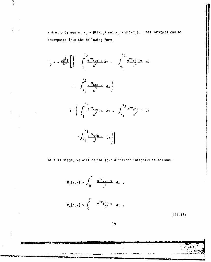
where, once again, x, - S(z-k1 ) and x 2 a(z-z 2 ). This integral can be

decomposed into the following form:

x

x2 x2

e cos u dd

xd

1 o_ 1

+ cos u dx2

f -U -2f U

cos U essin u dx

x I u 3I

At this stage, we will define four different integrals as follows:

x

M [ax] = e-UCos. u dx ,C0 u

x

M [a,x] = e Usin u dx

(111.16)

19

II• I ~ lI I~l I~ i • ''I• -• - - =II' . .. _ ... _J LIL . .. . ... ... . .. i l, - -- I I "r._ __ .. .... ... .... .. .. ... t :( •o L,-

x

N e-Uosn u dx

N5 [a,x]dx

N a]=f e-Usin Y dx

Using these integrals, the magnetic field expression can be written as

4o--- J[Mc[a, x2] Mca, X] + Ms[a, x2 ] Ms[a, x1]

+ Nc[a, x2] - Nc[a, xil}

+ I Mc[a, x2] _ Mc[a, xlJ . Ms[a, x2] + Ms[a, X] i-Ns[a, x2 ] + Ns a, xil] (I1l.17)

with the corresponding component of magnetic induction B being given

by the usual expression

B'ý Z 10 H I l . 8,

111.3 Parametric Approach

As shown by Fraser-Smith and Bubenik [1979], we can make use of a

parametric approach by normalizing all the distances in our expressions

by the skin depth of the surrounding conducting medium, 6, where

20

6 =(2/w.ijo)½

Using this technique, Equations (III.10), (1l1.11) and (111.17) can be

written in the following forms:

2 [(1+i)r 26 -(1 +i)r 162 e•, e

a 6 E = ((l+i)r 2 6+1 - e (o+i)r 6 +lI, (1Il.19)r 26 r16

i 6IE zinh 626 - sinh -I 6"16c 2z *= sin •8p 6

c E ['P69 (z,-' 26)] + c~ [p6' (z6-ý169J1

- E S 1%0 ' (z 6-Z26) 1- E 5 f%' (z&.2'lz{1 j

e -[(1+i)r 2 5 (e+~r61 (z6 ~i26 1

26 16

((1+i)r16 +1) (z6- 'l6) (111.20)

21

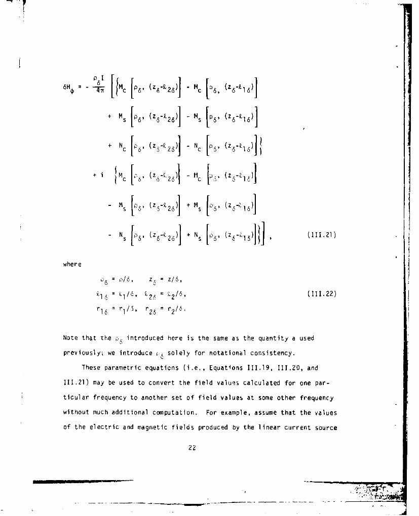
* 47 [I( C [i 6 5Z '26 ) ' C [56, &z6 'l66H4•

i-Mc [po6 , (zs-&.2s) - N z~i)

+ Ms [P6, (z5-k 2 6 )] -M s [P6, (z6-,16)l

where *Z6

+ l 2N = N [2/6" (II1.22)

rl6 = rI/S, r 26 = r 2/6.

Note that the p• introduced here is the same as the quantity a usedpreviously; we introduce ¢6 solely for notational consistency.

These parametric equaticns (i.e., Equations 1ll.19, I1I.20, and

111.21) may be used to convert the field values calculated for one par-

ticular frequency to another set of field values at some other frequency

without much additional computation. For example, assume that the valuesof the electric and magnetic fields produced by the linear current source

22

prvosy weitoueo oeyfr oainlcnitny

These~~~~~~~ ~ ~ ~ ~ ~ ~ paaerceutos ieEutos11.9°1.0 n

I- -

at the observation point P(p, ¢, z) in Figure III. are known for a

certain frequency f 1 " Let these field values be Ep M Epl, Ez Z Ezl

and B, = Bl respectively. If we now change the frequency by a factor

I/A 2 to f 2 fl/A2 the new skin depth will be 62 = A6S. If we multiply

all the distance coordinates in Figure III.' by A, i.e., change I' k2'

c, and z to Az,, At2, AP, and Az, then all the normalized distances in

the parametric equations stay the same and the electric and magnetic

field components at the new observation point P (Ap, c, Az) produced by

the linear current source extending from Z = AZI to Z AZ2 and operating

at the new frequency f2 2 = E = /A2 , Ez2 = Ezl/A2 and

B =2 - B4)1/A. These new field values for frequency f 2 can obviously be

calculated more easily from the field values for frequency fl than they

can from the original integral expressions.

111.4 Computations of the Fields

The expressions derived in Sections 111.1 and 111.2 for the field

components Ez and B contain integrals which in general can only be

evaluated numerically. As mentioned in Section Ill.1, there are a limit-

ed number of tabulated values available [Staff, 1949] for the two inte-

grals E ca,x] and E sa,x] in the expression for Ez, but there are no

tabulated values for the four integrals Mc[a,x], Ms[a,x], N c[a,x], and

N s[a,x] in the expression for B We therefore prepared two computer

programs for evaluating (1) the two components of the electric field,

E and Ez, and (2) the component of the magnetic field, B . In these

programs the six constitutive integrals in the field expressions were

23

evaluated numerically by means of Weddle's rule (Scarborough, 1966, p.

138). Both programs were interactive in the sense that the value of a

field component could be evaluated by entering the location and the

length of the linear current source, the amplitude and the frequency of

the current flowing in the source, and the coordinates of the observa-

tion point in the surrounding conducting medium.

The values for the numerical integrals were checked in several dif-

ferent ways. One obvious way was by comparing our computed results for

E c[a,x] and E s[a,x] with the available tabulated values (Staff, 1949].

Another way was to see if the values of the integrals converged to the

values tabulated for Kelvin functions and their derivatives [Young and

Kirk, 1964; Lowell, 1959; see Appendix B] for large values of the upper

limit of these integrals. We also used Simpson's rule [Scarborough,

1966, p. 137] and compared the values obtained by two different methods

of numerical integration; namely, Weddle's rule and Simpson's rule. In

all cases our computed values agreed well with the comparison values.

Shown in Figures 111.2 to 111.7 are computed values of the electric

and magnetic fields produced at frequencies of 100 Hz (Figures 111.2,

111.4 - 111.7) and 1 Hz (Figures 111.3, 111.8) by a linear current

source of 100 m length carrying an alternating current of 1000 A ampli-

tude. The fields are shown in two dimensions; in all cases the fields

are cylindrically symmetric about the axis defined by the source. Fig-

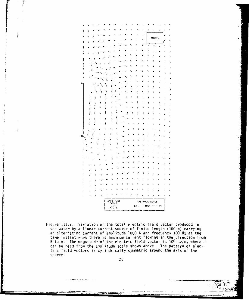
ures 111.2 and '11.3 show the spatial variations of the total electric

field vector at the instant when there is maximum current (O00A) in

the source flowing from B to A. The shorter wavelength at 100 Hz can

24

be clearly seen when comparison is made of the two figures. Figure

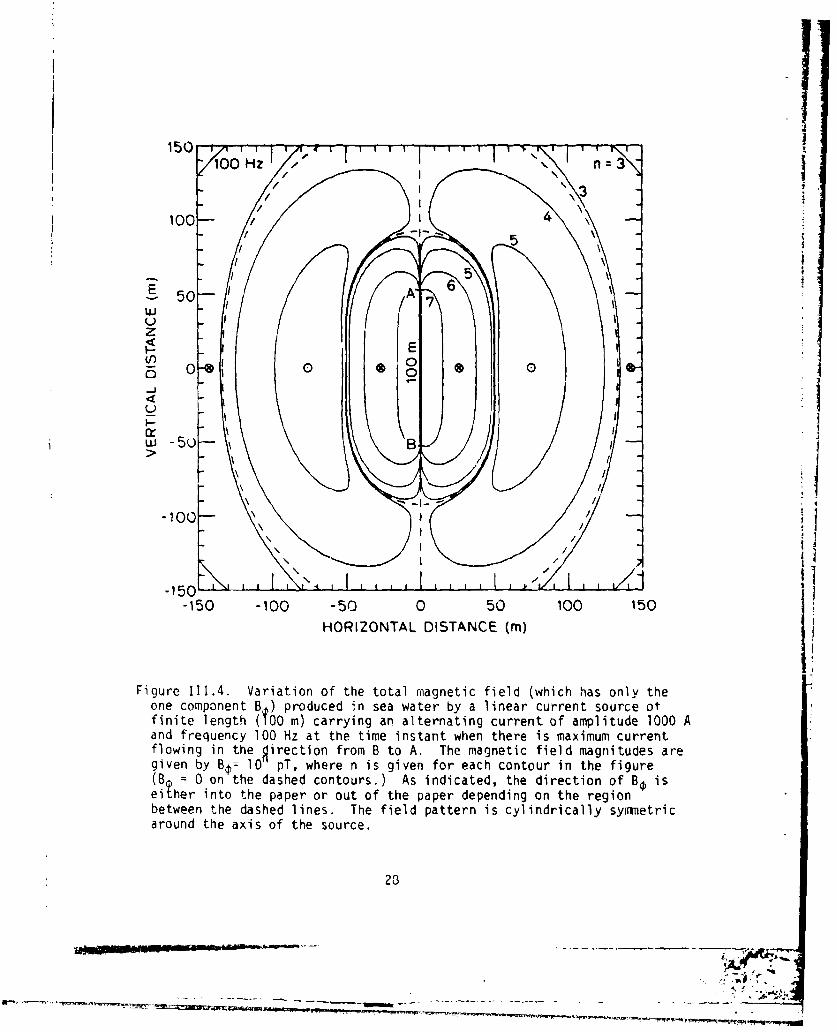
111.4 shows equal amplitude contours of the magnetic field component B,

for a frequency of 100 Hz at the time instant of maximum current flow

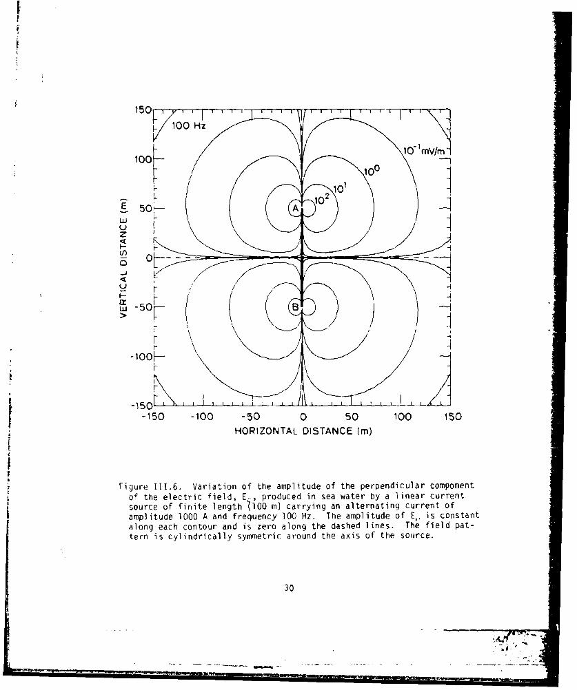
from B to A. Figures 111.5 and 111.6 show contours of the maximum

values reached by the t~o components of the electric field E and E

during one cycle of the source current. The dashed contours indicated

zero amplitude; thus in Figure 111.6 the E component is zero along thep

axis of the source and along the perpendicular line through the center

of the source. Comparing the two electric field figures, it is easy

to see how the two separate components Ez and E contribute to the total

electric field.

In Figure 111.7 we have drawn contours indicating the maximum values

reached by the 100 Hz total magnetic field variation at each point during

one cycle. Thus at points inside the contour labelled 104 pT, our data

show that the total magnetic field (or, equivalently, the magnetic field

component B ) will reach a values of 104 pT or more during one cycle of

the source current.

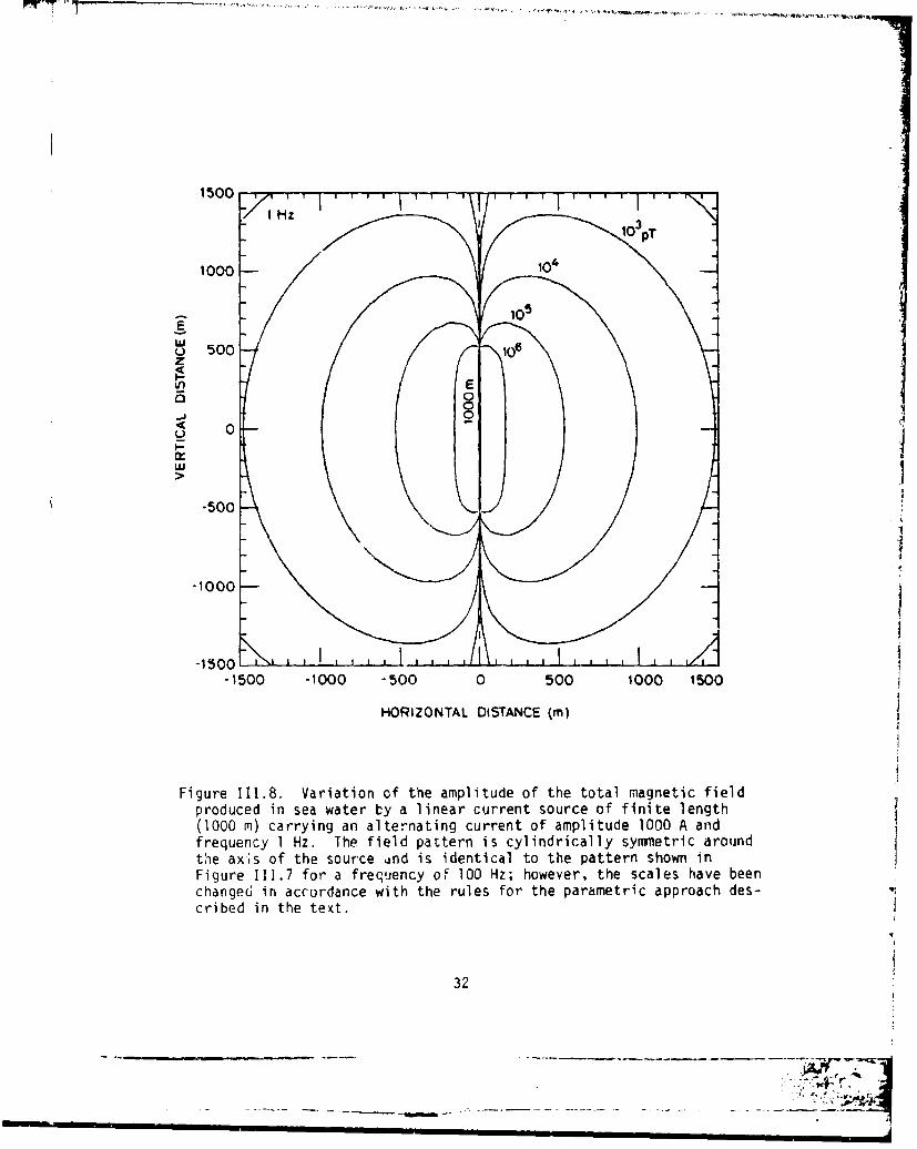
In Figure 111.8 we have relabelled tne data in Figure 111.7 accord-

ing to the parametric approach described in Section 111.3; the frequency

has been decreased by a factor of 100, the distances have been increased

by a factor of 10, and the values of B@ on the contours have been

decreased by a factor of 10. These changes leave the basic figure un-

altered, but the various contours now show maximum total magnetic field

values produced by a source of 1000 m length carrying a 1000 A alterna-

ting current with a frequency of 1 Hz.

25

AP IT D A L E :4 I -a j 4

--: / \ . ,- 4.. X I

Fiur 11.2 Vaito of th toa elcti fil veto prdue in

4 -

se ae y a liea curn sorc of fiit legt (10 m)cryn

B- to A . 4.e maniud of th elcti fil vetri 01iv hr

can ~ ~ ~ N be4

rea fro the amltd scl hw*bv.Tepteno lc

+ , ,+ * 4 ,i 4 4

4 4

Sf v a, t a s o

- - ., a .4 a

4 . ' . - - a A a $ 4

J I t•u, DISTANrCE SCAtI.

4.-.-- 50o .-~--.4 I

Figure 111.2. Variation of the total electric field vector produced in=

sea water by a linear current source of finite length (100 m) carryingan alternating current of amplitude 1000 A and frequency 100 Hz at thetime instant when there is maximum current flowing in the direction fromB to A. The magnitude of the electric field vector is I0 n uiv/m, where ncan be read from the amplitude scale shown above. The pattern of elec-tric field vectors is cylindrically symmnetric around the axis of thesource.

26

%s+'+ •

iA

, - .. _____ - - • .• 0 I . .

9 ,9 ." / 9 /"4 / ," '" -. - . s .

4 4 4 ,9 I - V . - A'

I ! ,# / / / . . . .

if ///, A .'" I -

/, / /..-.. - -

/I / i/ / o" " -'

I / / A - I. 1- / -'_, - -1 -/ .- .

A - .. --.-.. ,..-.- . ' .. N. . / N N " ,' /

"N '.. ' * . " ," \ ' I \ 1

\, \ 'N , N Nl 'N\ ".x N \i \. \

AMPLITUDE DITANCE SCA LE

Figure 111.3. Variation of the total electric field vector produced insea water by a linear current source of finite length (100 m) carryingan alternating current of amplitude 1000 A and frequency 1 Hz at thetime instant when there is maximum current flowing in the directionfrom B to A. The magnitude of the electric field vector is Ion Wv/m,

• where n can be read from tne amplitude scale shown above. The patternof electric field vectors is cylindrically symmetric around the axis

of the source .•2

''A

150 'z

100- 4

S50

w

z

w -5

0 I O

ULJB

I-10

-150 -100 -50 0 50 100 150HORIZONTAL DISTANCE (m)

Figure 111.4. Variation of the total magnetic field (which has only theone component B ) produced in sea water by a linear current source otfinite length (OO m) carrying an alternating current of amplitude 1000 Aand frequency 100 Hz at the time instant when there is maximum currentflowing in the girection from B to A. The magnetic field magnitudes aregiven by Ba,- 10 pT, where n is given for each contour in the figure(B - 0 on the dashed contours.) As indicated, the direction of B0 iseither into the paper or out of the paper depending on the regionbetween the dashed lines. The field pattern is cylindrically symmetricaround the axis of the source.

23

• __• : - _; . . . . . . .. . . .. .. • -. . .. .. -..-.j,,." r. ,

150

100 Hz it mVEzi

~~10

LU

z

0-00-

-150 d I

-150 -100 -50 0 50 100 150HORIZONTAL DISTANCE (in)

Figure 111.5. Variation of the amplitude of the parallel component ofthe electric field, Ez, produced in sea water by a linear currentsource of finite length (100 m) carrying an alternating- current ofamplitude 1000 A and frequency 100 Hz. The amplitude of E4isconstant along each contour. The field pattern is cylindrically sym-metric around the axis of the source.

29

•--- .. ..... .... , ---_7 1: ..

I,

SHz

100,-

F0

10 2-50-

r

-150 -100 -50 0 50 100 150

HORIZONTAL DISTANCE (m)

Figure 111.6. Variation of the amplitude of the perpendicular componentof the electric field, E-, produced in sea water by a linear currentsource of finite length (100 m) carrying an alternating current ofamplitude 1000 A and frequency 100 Hz. The amplitude of Ei, is constantalong each contour and is zero along the dashed lines. The field pat-tern is cylindrically symmetric around the axis of the source.

30

* .

150

1`ý00 Hz

iop

10*pT _

100

501

LU

z

U 50I-,-

1 - 0 1 I I1-.

-JB

-150 -100 -50 0 50 100 150

HORIZONTAL DISTANCE (M)

Figure 111.7. Variation of the amplitude of the total magnetic field(which has only the one component BO) produced in sea water by alinear current source of finite length (100 m) carrying an alternat-ing current of amplitude 1000 A and frequency 100 Hz. The fieldpattern is cylindrically symmetric around the axis of the source.

31

1500

1000- 0

S~105

u 500z

o_ 0

LU

*500

-1000

-1500 -1000 -500 0 500 1000 1500

HORIZONTAL DISTANCE (M)

Figure 111.8. Variation of the amplitude of the total magnetic fieldproduced in sea water by a linear current source of finite length(1000 m) carrying an alternating current of amplitude 1000 A andfrequency 1 Hz. The field pattern is cylindrically symmetric aroundthe ax;s of the source und is identical to the pattern shown inFigure 111.7 for a frequency oil 100 Hz; however, the scales have beenchanged in accordance with the rules for the parametric approach des-cribed in the text.

32

SI* .. -I l

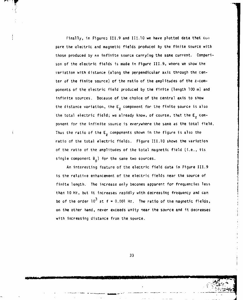
Finally, in Figures 111.9 and I11.10 we have plotted data that cur;

pare the electric and magnetic fields produced by the finite source with

those produced by an infinite source carrying the same current. Compari-

son of the electric fields is made in Figure 111.9, where we show the

variation with distance (along the perpendicular axis through the cen-

ter of the finite source) of the ratio of the amplitudes of the z-com-

ponents of the electric field produced by the finite (length 100 m) and

infinite sources. Because of the choice of the central axis to show

the distance variation, the Ez component for the finite source is also

the total electric field; we already know, of course, that the Ez com-

ponent for the infinite source is everywhere the same as the total field.

Thus the ratio of the Ez components shown in the figure is also the

ratio of the total electric fields. Figure III.10 shows the variation

of the ratio of the amplitudes of the total magnetic field (i.e., its

single component B ) for the same two sources.

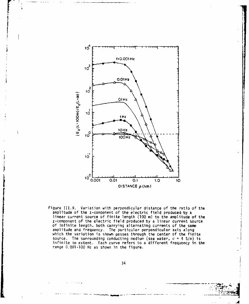
An interesting feature of the electric field data in Figure 111.9

is the relative enhancement of the electric fields near the source of

finite length. The increase only becomes apparent for frequencies less

than 10 Hz, but it increases rapidly with decreasing frequency and can

be of the order l10 at f = 0.001 Hz. The ratio of the magnetic fields,

on the other hand, never exceeds unity near the source and it decreases

with increasing distance from the source.

33

4' .

410

fQO.001 Hz

310

0.01HZ

2

0.1Hz

wS 1

E 10

0 ,, O~1HZ

0

,-5

N

S1OHz

w 0- 10

-1

10

II

0.001 0.01 0.1 1.0 10DISTANCE p (km)

Figure 111.9. Variation with perpendicular distance of the ratio of theamplitude of the z-component of the electric field produced by alinear current source of finite length (100 m) to the amplitude of thez-component of the electric field produced by a linear current sourceof infinite length, both carrying alternating currents of the sameamplitude and frequency. The particular perpendicular axis alongwhich the variation is shown passes through the center of the finitesource. The surrounding conducting medium (sea water, a = 4 S/m) isinfinite in extent. Each curve refers to a different frequency in therange 0.001-100 Hz as shown in the figure.

34

. '. . I, .

1011

10

-- < f 100 Hz

E0o 10 Hz~100

--Hz

"111,1, , ,,, , , , ,, ,, , , ,, ,, , 0I," , ,,

00

tO0.001 0.01 0. 1 1.0 10

DISTANCE p (kW)

Figure 111.10. Variation with perpendicular distance of the ratio ofthe amplitude of the magnetic field produced by a linear currentsource of finite length (100 m) to the amplitude of the magnetic fieldproduced by a linear current source of infinite length, both carryingalternating currents of the same amplitude and frequency. The parti-cular perpendicular axis along which the variation is shown passesthrough the center of the finite source. The surrounding conductingmedium (sea water, a = 4 S/m) is infinite in extent. Each curverefers to a different frequency in the range 0 - 100 Hz as shown inthe figure.

35

S. . .. '1 . . -_ . . .. .. . . . . . . . i-• - . . . .... -'~ 'Gy. 1 , -

IV. LINEAR CURRENT SOURCE OF INFINITE LENGTH

IV.l Derivation of the Field Expressions

In the preceding section we derived expressions for the electric

and magnetic fields produced in a conducting medium of infinite extent

by a linear current source of finite length. In the coordinate system

of Figure III. the wire extended from z to 12 in the z direction.

Suppose now that we let 9,, go to -- and '2 go to +-. The electric field

components given by Equations 111.5 then become

E =0,

Ez = -1f P(r)d.

Thus the electric field of a linear current source of infinite length

aligned in the z direction has only a z-component. Making the same

substitution as in Section 11, the expression for Ez can also be

written as

E LO = I#L'f -0 I udx,Ez -u d

where u = (a2 + 2 x2 ). Knowing that the integral in this equation is an

even function of x, we can also write

-(1+i)u= i7 Jo e dx (IV.2)

As described in Appendix B, the integral can be replaced by the modified

37

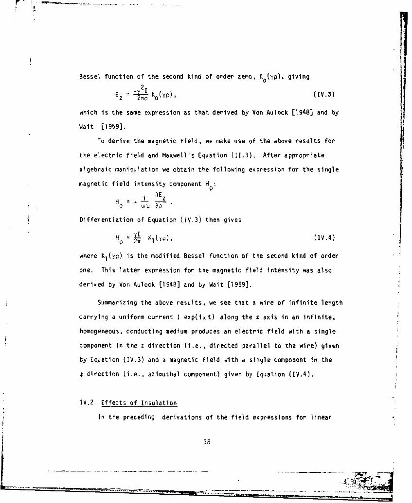
Bessel function of the second kind of order zero, K (yp), giving

Ez = -Y Ko(yw), (IV.3)

which is the same expression as that derived by Von Aulock £1948) and by

Wait [1959).To derive the magnetic field, we make use of the above results for

the electric field and Maxwell's Equation (11.3). After appropriate

algebraic manipulation we obtain the following expression for the single

magnetic field intensity component H :

- i ýE zH -

Differentiation of Equation (iV.3) then gives

Hý = Y K , (IV.4)

where KI(yo) is the modified Bessel function of the second kind of order

one. This latter expression for the magnetic field intensity was also

derived by Von Aulock [1948] and by Wait [1959].

Summarizing the above results, we see that a wire of infinite length

carrying a uniform current I exp(iwt) along the z axis in an infinite,

homogeneous, conducting medium produces an electric field with a single

component in the z direction (i.e., directed parallel to the wire) given

by Equation (IV.3) and a magnetic field with a single compooent in the

@ direction (i.e., azimuthal component) given by Equation (IV.4).

IV.2 Effects of Insulation

In the preceding derivations of the field expressions for linear

38

current sources of finite and infinite length we assume that tiie current

is uniform throughout the length of the conducting wire comprising the

actual source and that it flows into the conducting medium only from the

ends of the wire. For this condition of uniform current to apply, it is

of course necessary to have insulation on the wire. Without insulation

the current in the wire would flow into the surrounding conducting me-

dium from all points of the wire's surface, and uniform current flow

along the length of the wire could not be achieved.

Extending results obtained by Sunde [1949], Wait [1952] states that

the propagation constant for low frequency currents in an insulated wire

in a conducting medium is determined largely by the electrical character-

istics of the insulation, and he gives the following approximate expres-

sion for the current I(x) at a point in the wire located a distance x away

from the generator terminals:

l(x) z 1Io exp (-rx),

where I is the current assumed to be entering the wire. The propagation0

constant r in this expression is given approximately by

r z i(cu 2l)

where c and Wi are the permittivity and permeability of the insulation

material. It follows from these expressions that the current along an

insulated wire of length L will be essentially uniform provided IrLj << .

Suppose we take polyethylene to be a typical insulating material. For

this material we can write ci - rco' with er = 2.25 (the dielectric con-

stant of polyethylene), and p - Wo" Substituting the known values of

39

E and lio we obtain

irl - (3.14 x 108 f) mnl

Fir f -1 Hz, Irl ' 3 x 1O8 m- and the length of wire can be as

large as 1000 km and yet the condition IrLI << 1 is still satisfied.

Thus for low frequencies and typical insulating materials, it is reason-

able to assume that an alternating current is uniform throughout the

length of a wire for wire lengths varying from several hundreds to

several thousands of kilometers.

It also follows that the displacement currents flowing to the

surrounding medium through the insulation are negligible and the current

mostly flows to the medium from the ends of the wire.

It is also shown analytically by Wait [1952] and stated by Kraich-

man [1976] that the electric and magnetic field expressions for linear

current sources of both finite and infinite length (with the wire

assumed to be of negligible thickness in both cases) are unaffected by

the properties of the insulating material on the wire as long as the

ratio of the radius of the insulation to the wavelength of the surround-

ing conducting medium is much less than one. This condition can be

written in the form

<< 1,

where b is the radius of insulation and 1, and a are the permeability and

the conductivity of the surrounding medium. For sea water (a = 4 S/m,

= o= 41r x 107 H/m) this condition becomes

40

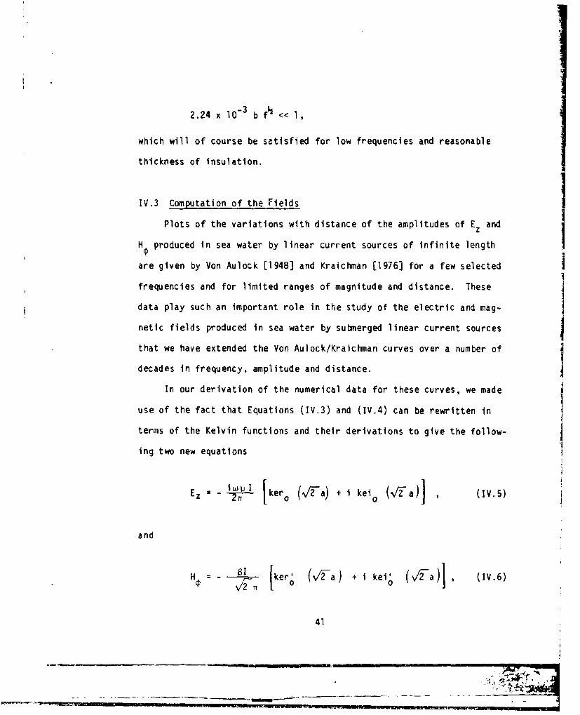
2.24 x 10-3 b f0 << I,

which will of course be satisfied for low frequencies and reasonable

thickness of insulation.

IV.3 Computation of the Fields

Plots of the variations with distance of the amplitudes of Ez and

H produced in sea water by linear current sources of infinite length

are given by Von Aulock [1948] and Kraichman [1976] for a few selected

frequencies and for limited ranges of magnitude and distance. These 4

data play such an important role in the study of the electric and mag-

netic fields produced in sea water by submerged linear current sources j

that we have extended the Von Aulock/Kraichman curves over a number of

decades in frequency, amplitude and distance.

In our derivation of the numerical data for these curves, we made

use of the fact that Equations (IV.3) and (IV.4) can be rewritten in

terms of the Kelvin functions and their derivations to give the follow-

ing two new equations

i W V I I 'a) ke--- kero (/-a) + i ke ° (, -a) , (IV.5)

and

H - [ ker0 (v/2-a + i kei, a (IV.6)

41

- . -------*-

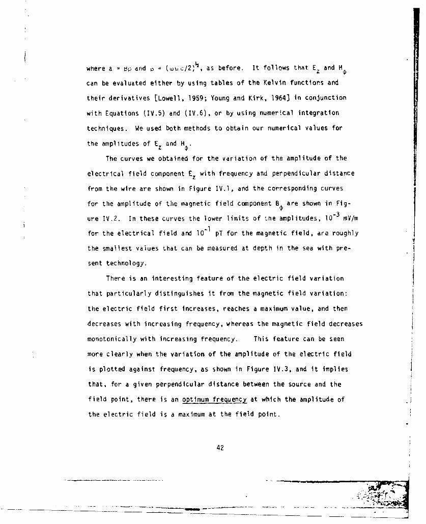
where a = tp and p = (wuc/2)'½, as before. It follows that Ez and H

can be evaluated either by using tables of the Kelvin functions and

their derivatives [Lowell, 1959; Young and Kirk, 1964] in conjunction

with Equations (IV.5) and (IV.6), or by using numerical integration

techniques. We used both methods to obtain our numerical values for

the amplitudes of Ez and H.

The curves we obtained for the variation of the amplitude of the

electrical field component Ez with frequency and perpendicular distance

from the wire are shown in Figure IV.l, and the corresponding curves

for the amplitude of the magnetic field component B are shown in Fig-

ure IV.2. In these curves the lower limits of the amplitudes, 10" mV/m

for the electrical field and 10-1 pT for the magnetic field, are roughly

the smallest values that can be measured at depth in the sea with pre-

sent technology.

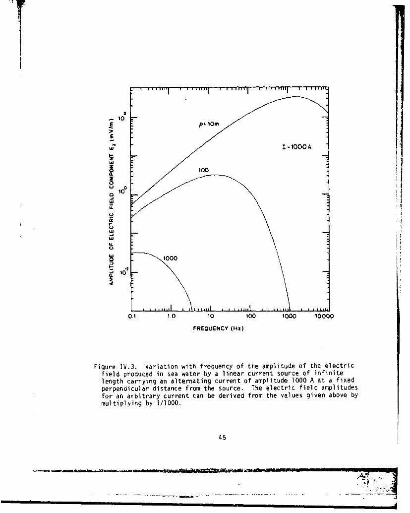
There is an interesting feature of the electric field variation

that particularly distinguishes it from the magnetic field variation:

the electric field first increases, reaches a maximum value, and then

decreases with increasing frequency, whereas the magnetic field decreases

monotonically with increasing frequency. This feature can be seen

more clearly when the variation of the amplitude of the electric field

is plotted against frequency, as shown in Figure IV.3, and it implies

that, for a given perpendicular distance between the source and the

field point, there is an optimum frequency at which the amplitude of

the electric field is a maximum at the field point.

42

@104

I I It100 Hz

EI

E f•"O z I :=1000AE

S10100W

~i 2 Hoz 10=---•owz0

0

WC-J)

o 10

U

- \1 - 0

L)w"--w

0wo' -2• --.-- Ll•:

UU

0.001 0.01 0.1 1 10DISTANCE (kin)

Figure IV.l. Variation with perpendicular distance of the amplitude ofthe electric field produced in sea water by a linear current sourceof infinite length carrying an alternating current of amplitude l000A.The electric field amplitudes for an arbitrary current I can bederived from the values given above by multiplying by 1/1000.

43

I- .44A

I I I Till I ~r7-r-nlTlT--T -r-M T1

1: 1000 AI-

10

zwz0

0

IL

f- f=1000Hz 100 10\. 0.1 00\ .001

z E

\ \ \\ \

IL

I 111 I * I IIII .1 1 11111 11111 1 1.

0.001 0.01 0.1 1.0 10 100DISTANCE (kin)

Figure IV.2. Variation with perpendicular distance of the amplitude ofthe magnetic field produced in sea water by a linear current sourceof infinite length carrying an alternating current of amplitude 1000 A.The magnetic field amplitudes for an arbitrary current I can bederived from the values given above by multiplying by I/1000.

44

Iq

- 10E ps IOM

E

"I'IO00A

2-)

100

1000

-2LA

U- I i l al

o

- -2

tO

0.1 1.0 10 100 1000 10 00FREQUENCY (Hz)

Figure IV.3. Variation with frequency of the amplitude of the electricfield produced in sea water by a linear current source of infinitelength carrying an alternating current of amplitude 1000 A at a fixedperpendicular distance from the source. The electric field amplitudesfor an arbitrary current can be derived from the values given above bymultiplying by I/1000.

45

AA

-;w~

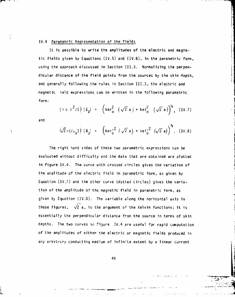
IV.4 Parametric Representation of the Fields

It is possible to write the amplitudes of the electric and magne-

tic fields given by Equations (IV.5) and (IV.6), in the parametric form,

using the approach discussed in Section I1l.3. Normalizing the perpen-

dicular distance of the field points from the sources by the skin depth,

and generally following the rules in Section III.3, the electric and

magnetic ield expressions can be written in the following parametric

form:

(T.o $2/i/) Ezi (kero (112-a) + keio (2-a))½, (IV.7)

and

(v/2-,/6 J) BI (kero2 (V2-a) + keio2 (V1a)) (IV.8)

The right hand sides of these two parametric expressions can be

evaluated without difficulty and the data that are obtained are plotted

in Figure IV.4. The curve with crossed circles gives the variation of

the amplitude of the electric field in parametric form, as given by

Equation (IV.7) and the other curve (dotted circles) gives the varia-

tion of the amplitude of thE magnetic field in parametric form, as

given b) Equation (IV.8). The variable along the horizontal axis in

these figures, V/2a, is the argument of the Kelvin functions; it is

essentially the perpendicular distance from the source in terms of skin

depths. The two curves i,- Figure IV.4 are useful for rapid computation

of the amplitudes of either the electric or magnetic fields produced in

any arbitrary conducting medium of infinite extent by a linear current

46

;71,P

S.. . . . .° -7

-~~1 3- -------

- ..~

00 2

101

lop

10

-I0

"C4

b103

105

.6o0 0" 107 10 10 10 t02

Figure IV.4. Variation with parametric distanceF2a (where a P6

p/6) of the parametric expressions for the amplitude of the electric

field (crossed circles) and the magnetic field (dotted circles) pro-

duced in a conducting medium of infinite extent by a linear current

source of infinite length carrying an alternating current of amplitude

I.

47

___

source of infinite length over a very wide range of source currents

and frequencies. For example, if the observation point is 100 m away

(perpendicular distance) from the source and the source frequency is

1 Hz, we have i2a = 0.56 and using Figure IV.4 we obtain approximately

1.0 and 1.6 for the parametric electric and magnetic field quantities

given on the vertical axis of the figure. Knowing that 6 = 251.6 m for

f = 1 Hz, o = 4 S/m, and =o 4ff x 107 H/m, and using I 103 A, we

obtain IEzI = 1.26 mV/m and IB I = 1.80 x 106 pT. These particular

values can be checked against the values of IEzI and IB I plotted in

Figures IV.l and IV.2.

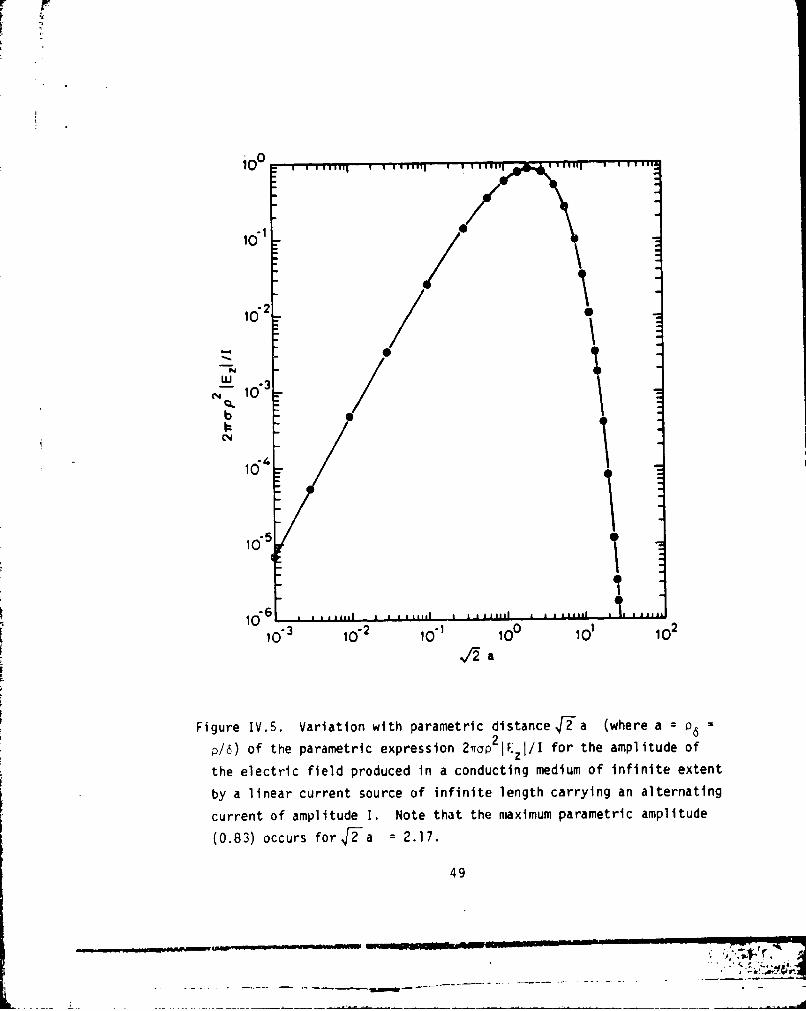
We have also plotted in Figure IV.5 the amplitude of the electric

field in the alternate parametric form

2 ½

(2.Too2/I) JEz : ( v-a) ( ker2 (/-Ta) + ke12o(V/-2a)) .(IV.9)

This is basically the same equation as Equation (IV.7), except that in

Equation (IV.7) the left hand side is not a function of the perpendicu-

lar distance p and the left hand side of the above equation is not a

function of frequency. In other words, the single curve shown in Fig-

ure IV.5 is a parametric form of the curves seen in Figure IV.3; it

contains all their information on the variation of the amplitude of the

electric field with perpendicular distance and source frequency, as

well as much additional information of the field amplitudes at other

distances. (If required, the field amplitudes can also be computed in

other media than sea water.) The maximum value of the parametric electric

field expression occurs for V,/Ta = 2.17. This is a useful result to

48

-C31

10"

CL./1075

w'/2- a

b

10- I0-2 ,p+100 010

Figure IV.5. Variation with parametric distance F2-a (where a = 06

p/6) of the parametric expression 21rap 2 1F.zI/ for the amplitude of

the electric field produced in a conducting medium of infinite extent

by a linear current source of infinite length carrying an alternating

current of amplitude I. Note that the maximum parametric amplitude

(0.83) occurs for F2-a = 2.17.

49

remember, because it enables the optimum frequency of operation mentioned

in the previous section and the corresponding maximum electric field

to be computed. The procedure to obtain this information is as follows.

First, knowing the location of the observation point (i.e., the perpen-

dicular distance p), It is simple to obtain the frequency maximizing the

amplitude of the electric field at that specific point from jr2"a =

,[- p/6 = 2.17. This is the frequency we will refer to as the opti-

mum frequency. Next, the data in Figure IV.5 show that the maximum

value of the parametric electric field expression 2-apI2 EEzI/I is approx-.

imately 0.83, from which the actual value of the electric field ampli-

tude can be computed.

51

Ii

50

-S.

V. LINEAR CURRENT SOURCE OF SEMI-INFINITE LENGTH

V.1 Derivation of the Electric and Magnetic Field Components

In the previous section we obtained expressions for the electric

and magnetic fields produced by a linear current source of infinite

length by letting Z 1 and 1.2 tend to minus infinity and infinity, respec-

tively, in the expressions for the fields produced by a linear current

source of finite length. In this section we concentrate our attention

on the electric and magnetic fields surrounding the end of a linear

current source immersed in a conducting medium of infinite extent, i.e.,

around an electrode of negligible size in the medium. We do this by

letting just one end of the finite linear current source tend to infi-

nity, thus producing a linear current source of semi-infinite length.

Starting with the finite source electric and magnetic fields ex-

pressions (Equations 111.5 and 111.12), letting Z, go to --, and gen-

erally following a similar approach to the one used in Sections III and

IV, we obtain the following three expressions for the non-zero fields

in the conducting medium:

E = e-Yr 2

r2 (yr 2 + ), (V.1)

E [Isinh'1 x- Ec La, x2 ] - kero (J2-a)}

-i IE5 L a, x2) +; kei0 (/aJ

o i ~

I e'yr2

+ e---y (yr 2 + 1) (z - £2), (V.2)r2

and

Hr [ McEa, x2) + Ms[a, x2, + Nj[a, x2 31

+1 iM [a. x2 -M[a, x2) - N5Ea, x2)1

[ ker. 0 Ya + ikei,, (J2 a] (V. 3)

where all the terms here are defined as in Section III.

When the observation point is on the axis ot the semi-infinite

wire (i.e., p o and z >Z2), the above expressions simplify greatly to

give

E =0,

E+ ip In + lnx2 + -n Ejo0. x2 -i ~E C0, X)

.a ll e l+)x2 + I (VA4)+4-•o x2 2 ')x+

H =0.

52

In these last equations ye is Euler's constant, which, to four signifi-

cant figures, is given by ye 0.5772. This constant is usually denoted

by the symbol y, but we have added the subscript e to distinguish it

from the y used here for the propagation constant. There is, of course,

no relation between Euler's constant ye and the propagation constant y.

V.2 Some Numerical Values

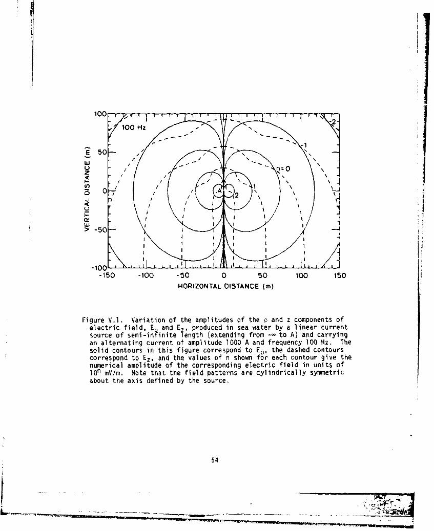
Figure V.1 shows contours of the maximum values reached by the two

components of the electric field, E (solid line) and Ez (dashed line)

around the end A of the semi-infinite source during one cycle of the

current in the source (the amplitude of the current is assumed to be

1000 A). As can be seen, there are some regions in the figure where

the p-component is larger than the z-component of the electric field,

but for large distances the z-component becomes by far the largest com-

ponent. This difference at large distances is caused by the overall

inverse cube decline of the p-component with distance (see Equation V.1),

in contrast to the z-component, which has only a partial inverse cube

dependence on distance (Equation V.2). Note that as the point of obser-

vation begins to move towards the other end of the source, i.e.,the end at

infinity, the z-component contours become parallel to the source and the

electric field values tend toward those produced by a linear current

source of infinite length.

53

100

t o- ,- N•l '•: -, -250 N

S/ /N/- • -•-o \"U nzz

sr o tWN

-100

-150 -100 -50 0 50 100 150HORIZONTAL DISTANCE (m)

Figure V.I. Variation of the amplitudes of the p and z components ofelectric field E• and E , produced in sea water by a linear currentsource of semi-in inite fength (extending from -- to A) and carryingan alternating current of amplitude 1000 A and frequency 100 Hz. Thesolid contours in this figure correspond to EP, the dashed contourscorrespond to Ez, and the values of n shown for each contour give thenumerical amplitude of the corresponding electric field in units ofIon mV/m. Note that the field patterns are cylindrically symmetricabout the axis defined by the source.

54

VI. LINEAR CURRENT SOURCE OF INFINITE LENGTH WITH A FINITE GAP

VI.l Derivation of the Fields

In Section IV we investigated the electromagnetic field produced

by an alternating current flowing in an insulated continuous linear

current source of infinite length immersed in a homogeneous conducting

medium of infinite extent. This system is distinguished by the fact

that all the impressed current is effectively confined to the source.

In other systems, for example linear current sources of finite or semi-

infinite length, the impressed current also flows into the surrounding

conducting medium from the ends of the wire. Suppose we now introduce

a gap into our linear current source of infinite length so that the

current in the scirfe is forced to flow through the conducting medium iover some finite distance. This system is equivalent to two semi-

infinite linear current sources carrying the same current and aligned

along the same axis but with a finite gap between them ds shown in

Figure VI.l(a).

We have already derived the electric and magnetic field expressions

for a semi-infinite linear current source, so, using superposition, we

can easily show that the fields produced by the system in Figure VI.l(a)

are given by the following equations:

e-r -yr1= E (yr2 + 1) - (yrI + 1) , (V1.1)r ( rI

Ez - [ker 0 (v/'2 a)+ i kei 0 (v'- a)I

55

+ +0

-CO -0

(a) (b)

Finure VI.l. Sketches of the two linear current sources of infinitelength with gaps that are considered in this work. In each case thegap extends from t = t1 to i = Z2 and the amplitude of L.,c current isthe same in both the upper and lower semi-infinite segments. However,the directions of the current flow are different in the two systems.In case (a) the currents flowing in each segment are in the samedirection, whereas in case (b) the currents are oppositely directed.

56

-IK ik

asinhl a sinh' a " Ec(a. x2) + Ec[a, xll

-i IEs[a, x2 ]- Es[a, Xl3

S e-yr', _____ +1( L ey y1(zZ(V.2-T -3-1 2[r ( \r 2 +l)(zL 2 ) r- e'Yrl J~~J

and

H = ~ ker' (.F2a) + i kei' (F/2 al

+ JM[a, x2 - Mc[a, xl] + M s[a, x2] -Msa, xl]

+ N [a, x2 ] -Nc[a, x1J,

+I IM c[a, x21 - Mc[a, x1] - Ms[a, x2 ] + Ms[a, x

- Ns[a, 2 + N xJ] (VI.3)s~a x2] N5Lap 11

It is interesting to note that, once again as a result of the prin-

ciple of superposition, these expressions can be derived by subtracting

the field expressions for a finite source of the same length as the gap

from the field expressions for the continuous source of infinite length.

Furthermore, if we are on the axis of the source and within the gap,

57

"H -1' • • -- m ,dl "I |~~~~ • - - - - --| ! mm - - -"

(i.e., p o and I1<z<2), the field expressions become

E = 0,

Ez = [2Ye + 1n2 + ln(-xlx2 )

+ E cO, x 2 ] - EC[O, xl]

+i I E s[0, x 23 - E5[0. x1i + T11 (VIA4)J

+ a 21 e-(l1~i (+i)x 1+I) e- -(l+i)x 2Xl x2

Hý 0.

A different version of this gap system can be obtained simply by

reversing the direction of the current in one of the semi-infinite seg-

ments, so that the currents are oppositely directed in the two segments

(Figure VI.l(b)). For this case, we can again make use of the semi-

infinite wire expressions to aerive the following electric and magnetic

field expressions:

~ e-Yr 2 +e-Yrl 1 vI5E = I er2 (yr 2 +l) + 7 (Yr 1 +l) (VI.5)

r r2 rlI

58

~ ;J

E 4i sinh' I + sinh1 a Ea' K2 ) - Ec a, x13

and

Hý 4-, lMe[a, x 2] + Me[a, xI] + Ms1a, x2] + Ms~a, X~l

+ N cE[a, x2] + Nc[a, Xl]1

- i imr[a, xyI + M2 [a, Xl] s[a, xe (r M [a, x( ]

S I r

"4 N J a, x2 - N Cja, X,]j L (VX.L )

As we will see in the following section, the fields produced by the two

gap systems have interesting differences in their properties.

VI.2 Numerical Results

As can be seen from the form of the field expressions VI.1 - VI.3

and VI.5 - VI.7, the spatial variations of the fields produced in and

around the two finite gaps considered in this work are not simple. To

illustrate these spatial variations, and to provide some representative

numerical data, we make the comparatively simple fields produced by a

59

continuous infinite linear current source our reference and we compare

the gap fields with these reference fields by computing ratios of the

corresponding field quantities.

The first of these comparisons is made in Figure VI.2. where we

have plotted the variation with perpendicular distance of the ratio of

the ampl'tudes of the total electric field produced by (a) the infinite

linear current source with a gap illustrated in Figu.e VI.l(a) (current

flow ng in the same direction in the two semi-infinite segments) and by

(b) the continuous infinite linear current source. The current is every-

where assumed to be the same in the sources, the gap width is taken to

be 100 m, and the variation with distance is taken along the perpendicu-

lar axis passing through the center of the gap. Because uf L•• choice

of this particular axis to show the distance variation, the j-component

of the electric 'ield produced by the gap system is zero at all the field

points that are considered and the total electric field and E are equi-

valent for both sources.

The most interesting feature of the data in Figure VI.2 is the

large ratio at small distances (i.e., p< 1000 m) for f < 1 Hz. At these

frequncies the amplitudL of the electric field in the vicinity of the

gap can be substantially larger than the amplitude of the field that

would be produced at the same locations by a continuous source carryino

the same current. The incrcase begins to decline rapidly once a minimum

perpendicular distanre is excceded. In Figure VI.2 this distance is

aporoximately 50 m, which also happens to be the distance from the cen-

ter of the gap to the r.ear ends of the two semi-infinite segments.

60

boom.-&~ -

10'

f 0.001 H z

"0.01Hz

ii 2

W ~0.1 Hz

o 100 1.0 Hz

0 90LV

* 0 10 -------------W 10.0 Hz

100.0 Hz

001 Q1 0.1 1.0 10

Figue V.2.Variation with perpendicular distance of the ratio of theamplitudes of the z-components of the electric field produced (a) bya linear current source of infinite length with a finite gap (100 in),carrying current flowing in the same direction in each semi-infinitesegment. and (b) by a continuous linear current source of infinitelength. Both sources carry alternating currents of the same amplitudeinci frequency and the perpendicular axis along which the distancevariation is shown passes through the center of the gap. The surround-ing conducting medium (sea water, o 4 S/rn) is assumed to be infinitein extent.

61

-I U A

WAN&NC-*.km

Beyond this minimum distance the ratio of the total field amplitudes

rapidly approaches unity, no matter what frequency is involved, and at

large distances the fields of the gap system approximate those produced

by the continuous linear current source of infinite length.

A second comparison of the gap fields with the reference fields pro-

duced ty a continuous source is made in Figure VI.3. In this figure the

gap is the same size (100 m) as in the previous example, but the currents

in the two semi-infinite segments are now taken in opposite directions.

The figure therefore shows the variation with perpendicular distance of

the ratio of the amplitudes of the total electric field produced by (a)

the infinite linear current source with a gap illustrated in Figure IV.

l(b) (current flowing in opposite directions in the two semi-infinite

segments) and by (b) the continuous infinite linear current source. As

ji before, the amplitude of the current is everywhere considered to be the

same in the sources and the variation with distance is taken along the

perpendicular axis passing through the center of the gap. Again because

of the choice of this particular axis to show the distance variation,

the electric fields produced by the gap system have a distinguishing

characteristic: the z-component of the electric field is zero at all

the field points that are considered and the total electric field and

E are equivalent. For the continuous source, the total electric fieldp

and Ez continue to be equivalent.

As was observed in the previous example, there is a region near the

gap where the ratio is much larger than one for the lower frequencies

(f < I Hz). This region extends out somewhat further from the gap than

62

0.001 Hz /

102Ui ,/ /,>>YZ,,,

0.0

"E 10

E 10 -- - - - - -0 /

10._l

O.310 2

0

100.0Hzz

3.310 1.

0.001 0.01 0.1 1 10

DISTANCE p (kin)

Fig. VI.3. Variation with perpendicular distance of the ratio of theamplitudes of (a) the p-component of the electric field produced by alinear length with a finite gap (100 m), with current flowing in oppo-site direction in each semi-infinite segment, and (b) the z-componentof the electric field produced by a continuous linear current sourceof infinite length. Both sources carry alternating current of thesame amplitude and frequency and the perpendicular axis along whichthe distance variation isshown passes through the center of the gap.The surrounding conducting medium (sea water, o = 4 S/m) is assumedto be infinite in extent.

63

Rwas observed before, which may be considered a positive characteristic of

this particular gap system's electric field. On the other hand, at large

distances the gap system's electric field decays more rapidly with dis-

tance than the electric field of the reference source and the ratio

plotted in the figure becomes less than one.

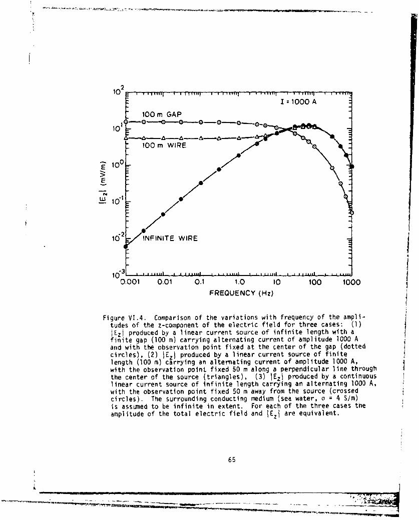
Our third and final comparison of the electric fields produced by a

gap system with the fields produced by other systems is made in Figure

VI.4. In this case we have plotted the variations with frequency of the

total electric fields produced at three different observation points, as

follows: (1) an observation point at the center of the gap system (gap

width - 100 m) illustrated in Figure VI.l(a); (2) an observation point

50 m away from the center of a linear current source (length - 100 m)

and located on a perpendicular lIne through the center of the source;

and (3) an observation point located 50 m away from a continuous linear

current source of infinite lengt:i (our reference source). In all cases

the amplitude of the current in the sources is lO0 A.

These final data show once again how the electric field of the

reference source can be exceeded substantially by the fields produced

either by gap systems or sources of finite length carrying the same total

current when the frequencies and distances are small. However, as the

field point distances increase and become large in terms of skin depths

the fields produced by the continuous linear current source of infinite

extent are at least as large as any of the other fields, and they may be

substantially larger in some cases.

64

kS. -• -4-yt • tr - • r~ _______ - - -w•-

10 2 1 , i , '- ! V ' 1 1w- ' ,1 , l ,m I ' 'I ,•1 I I ¢ ' I wlm l - I I ' I II,

! l mGA1 1000 A• 100 m GAPi

100 m WIRE

100

10 INFINITE WIRE

FI

0.001 0.01 0.1 1.0 10 100 1000FREQUENCY (Hz)

Figure VI.4. Comparison of the variations with frequency of the ampli-tudes of the z-component of the electric field for three cases: (1)jEzj produced by a linear current source of infinite length with afinite gap (100 m) carrying alternating current of amplitude 1000 Aand with the observation point fixed at the center of the gap (dottedcircles), (2) IEzj produced by a linear current source of finitelength (100 m) carrying an alternating current of amplitude 1000 A,with the observation point fixed 50 m along a perpendicular line throughthe center of the source (triangles), (3) )EzI produced by a continuouslinear current source of infinite length carrying an alternating 1000 A,with the observation point fixed 50 m away from the source (crossedcircles). The surrounding conducting medium (sea water, a = 4 S/m)is assumed to be infinite in extent. For each of the three cases theamplitude of the total electric field and lEzi are equivalent.

65

--- -I- I1_- --I--6- -- - - - - - - -

The electric and magnetic fields along the straight line joining

the two ends of the gap, i.e., along the axis of the gap, have a simple

vector form: the electric field has only a single component directed

along the axis and the magnetic field is zero. Unfortunately, this

simplicity does not carry over to the spatial variation of the electric

field along the axis. Further, just off the axis the magnetic field

has a non-zero azimuthal component, and this component also has a com-

plicated spatial variation as the observation point moves along a line

parallel to the axis. In general, both the axial electric field compo-

nent and the off-axis magnetic field component are large near the two

ends of the gap and they decrease as the observation point moves toward

the center of the gap. The magnitude of the decrease depends in parti-

cular on the width of the gap and on the frequency: if the gap width is

less than a skin depth, the decrease can be quite small; but if the

width exceeds a skin depth, the decrease can be very large near the

center of the gap. This behavior is well illustrated by the curve in

Figure VI.4 showing the variation with frequency of the amplitude of

the total electric field (i.e., the axial or z-component) at the center

of a 100 m gap in sea water. It can be seen that as the frequency in-

creases from 0.001 Hz there is little variation in the amplitude until

the frequency reaches about 4 Hz (skin depth = 125.8 m), but by the time

the frequency has reached 10 Hz (skin depth = 79.6 m) the amplitude has

noticeably begun to decline.

66

VII. LINEAR CURRENT SOURCE OF INFINITE LENGTH WITH AN ELEMENTARY GAP

In the previous section we derived the fields produced by two semi-

infinite linear current sources aligned along the same axis with a gap

between them. If we now reduce the size of the gap until it becomes in-

finitesimal, we will obtain a linear current source of infinite length

with an elementary gap in the middle.

Suppose the gap has an elementary length T and that it is centered

on the orgin. Starting from the Hertz vector expression for a current

element source (Equation Il1.2) and integrating it with the right limits,

we obtain the total Hertz vector due to the infinite length wire with an

elementary gap:

f-/2 -+ -yr

4- r 10---F-00 -/2- r

which can also be written in the form

+. +T/2O e"yr -yr (VII.?)

F. The two terms on the right of this last expression are easily recog-

nized: the First term is the Hertz vector due to a continuous infinite

linear current source and the second term is the Hertz vector due to a

current element of elementary length T.

Using Equations (II.5) and (11.6), the electric and magnetic fields

tor this system cart be derived with little difficulty; they are given by

the following expressions:

67

I ý

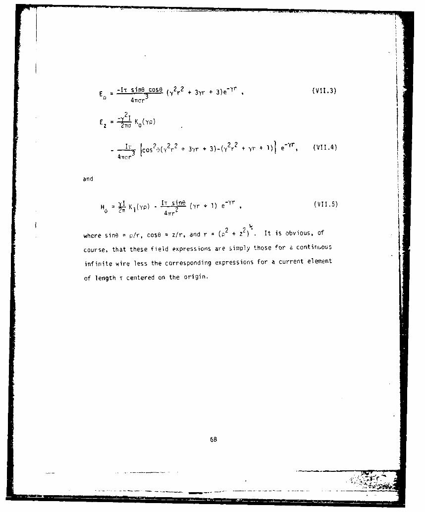
--IT sinO coSO 2 2 -yr-I4T-c -3 i r + 3yr + 3)er (VII.3)

4•c

2IEz= Ko(-y)

- l cos 23(Y 2r 2 + 3yr + 3)-(y 2 r 2 + yr + 1) eYr (VII)

and

I ) IT sine (V+I -yrHýr 2 (yr + 1) e"Ir

2 2where sine p/r, cosO = z/r, and r = (P + z ) It is obvious, of

course, that these field expressions are ýimply those for a continuous

infinite wire less the corresponding expressions for a current element

of length T centered on the origin.

68

S....... '--- 'ii " u'l . ....]ii ' i '-"i i i-'

VIII. SUMIMARY AND CONCLUSIONS

VIII.l Summary

Starting with the theoretical work of Von Aulock [1948, 1953], Wait

[1952, 1959, 1960], and Kraichman [1976], we have derived a number of

new theoretical arid numerical results for the ULF/ELF electromagnetic

fields produced in a conducting medium of infinite extent by a variety

of linear current sources. Many of the numerical results apply specifi-

cally to a sea water medium, since our work is oriented toward an under-

sea communication application, but the basic theory and some of the

numerical data for the parametric expressions are given in a form that

is independent of the specific conducting medium. The following is a

list of the new results we have derived; in all cases the sources and

observation points are taken to be in a conducting medium of infinite

extent:

(1) We have greatly expanded the available numerical data on the

electrical and magnetic field amplitudes produced by linear current

sources of infinite length for frequencies in the range O.OG - 1000 Hz.

We have also introduced a parametric representation for these fields and,

for any particular observation point, we have specified a technique for

deriving the optimum frequency, i.e., the frequency for which the ampli-

tude of the electric field is a maximum.

(2) We have extended the work of Wait (1952] on the electric fields

produced by a linear current source of finite length by deriving an ex-

pression for the single magnetic field component (the azimuthal component)

produced by such a source. We have also used a numerical integration

69

- - . . . - i " . . . . I_ IIZ 7

S.. . . II - "I I I • | I • I • | |

technique to obtain numerical values for the amplitudes of the electric

and magnetic fields produced in sea water by representative finite

sources.

(3) By extending one end of the finite source in (2) to infinity,

we have derived new expressions for the electric and magnetic fields

produced by a linear current source of semi-infinite length. Once again

using numerical integration, representative numerical values for the two

components of electric field have been c .ained around the end (a "point

electrode") of this semi-infinite source in sea water.

(4) By combining two of the semi-infinite sources described in (3),

we have derived expressions for the electric and magnetic fields produced

by a linear current source of infinite length containing a gap of finite

size. Two versions of this source are considered: (a)currents of equal

amplitudes flowing in the same directions in both semi-infinite segments,

and (b) currents of equal amplitudes flowing in opposite directions in

the two semi-infinite segments. Once again, representative numerical

values have been computed for the amplitudes of the electric fields and

the fields have been compared with those produced by an equivalent

continuous source of infinite length.

(5) Finally, we have reduced the size of the finite gap in (4)

until it is infinitesimally small and shown that the fields produced in

the vicinity of the elementary gap are equivalent to the fields produced

by a continuous linear current source of infinite length less the fields

produced by an elementary current source at the location of the gap.

In general, we have made as few assumptions as possible in deriving

70

the above expressions and numerical data. The assumptions that are made

can be summarized as follows. First, the displacement current is neg-

lected. This is a very good assumption at all frequencies up to about

100 MHz if the surrounding medium is sea water. Second, we assume that

the amplitude of the alternating current is the same throughout the

various sources. At the ULF/ELF frequencies that are considered, this

is equivalent to assuming that the current sources are insulated every-

where except at their ends. Third, we assume that the shortest distance

between any observation point and the surface of the sources (which are

tatken to be circular in cross-section) is always much greater than the

source radius. This assumption is discussed in greater detail in Appen-

dix A. Finally, as we have pointed out many times, the conducting medium

is always assumed to be infinite in extent.

VIII.2 Discussion

Our first objective in deriving the field expressions in Chapters

III, V, and VI for sources of finite and semi-infinite length, and of

infinite length with a gap of finite size, was to investigate the possi-

ble desirable characteristics of the fields near their open ends (i.e.,

point electrodes) for undersea communication at ULF/ELF frequencies.

Assuming that this first part cf our study gave positive results, our

second objective was to derive enough theory and numerical data to pro-

vide the basis for the preliminary design of undersea communication

arrays that would have the capability of producing measurable ULF/ELF

signals throughout limited regions of the ocean without the cables pro-

71

ducing the signals necessarily being located in the regions. To a large

extent our objectives have been achieved: comparatively large electric

and, to a lesser extent, magnetic fields can be produced at ULF/ELF fre-

quencies in the vicinity of the open ends of the sources considered in

this work, and measurable ULF/ELF fields can be produced in and surround-

ing the region of a moderately large gap in an otherwise continuous

current-carrying cable. However, it is important for us to point out

that the same frequency versus range constraint applies in the case of

the electromagnetic fields produced by urdersea cabies, and without

gaps, as is encountered in other methods of undersea communication in-

volving electromagnetic signal propagation in sea water: large ranges

can be achieved by using low frequencies, particularly low ULF frequen-

cies, but because the rate of data transfer is directly proportional to

the signal frequency, the rate of data transfer over the large ranges may

be too small to be useful. As we will now show, this frequency versus

range constraint effectively limits the use of discontinuous cable

arrays to short range comtnunication.

Comparing the ULF/ELF fields produced in sea water by cables of

finite and senmi-infinite length, and of infinite length with a gap, with

the fields produced by a long continuous current-carrying cable (our

linear current source of infinite length), our data show that at short

distances from their open ends i.e., distance; less than about 1 km, the

discontinuous sources can produce greatly enhanced electric fields. We

have not carried out a complete computation of all the field amplitudes

that can be produced under all possible circumstances, but the available

72

gr .•

IIi3

data indicate that the increase is confined largely to frequencies in

the ULF range and, within this range, it becomes larger as the frequency

is decreased. At 0.001 Hz, for example, the increase of nearly 2000

times that is observed at a perpendicular distance of 10 m from the cen-

ter of a 100 m gap in an otherwise continuous long current-carrying ca-

ble (Figure VI.2) is nearly 10 times larger than the increase at 0.01 Hz.

In all the cases we have examined the increase begins to decline rapialy

with distance once some limitino distance has been exceeded. For the

-wo gap systems discussed in Chapter VI the limiting distance is of the

same order as the width of the gap (100 m), a result that may be indica-

tive of a general relation at the low ULF frequencies under considera-

tion. It will be observed that the increase under discussion appears to

be confined to the electric field, as may be seen by comparinq the numeri-

cal data plotted in Figures 111.9 and I11.10 for the electric and magne-

tic fields produced by a cable of finite length. It is obvious from

these and the other results we have derived that discontinuous sources

have at best no advantage over the continuous linear source for field

generation at distances much above 1 km and, at worst, they may produce

much smaller fields than the continuous source for some geometries and

frequencies. We conclude therefore that arrays of finite and/or semi-

infinite cables, and continuous cable with gaps, can be used most advan-

tageously for undersea communication only over short distances.

The possible situatiors where such communication could be uwed are

not necessarily trivial. For example, the ULF/ELF electric fields around

the gap between two point electrodes, or near a single point electrode,

73

could provide a low-data-rate, non-acoustic means of communication with

an undersea or sea-floor receiver located beneath the hull of an elec-

trode or cable/electrode equipped ship. At the short distances under

consideration (distances < I km) there is likely to be no difficulty

providing communication with divers at frequen' *",• in the lower part of

the voice frequency range (50 - 3000 Hz); indeeu, a commercial unit has

been designed for an application of this kind [MacLeod, 1977]. As a

final note on the possi, e communication applications of the discontin-

,rcus sources, we observe that long range is not always a desirable fea-

ture cf a communication system, and under some circumstances the limited

ranges for signal propagation that we have discussed here could be a

decided advantage.

Turning now to the electromagnetic fields produced at large dis-

tances from the sources (distances of the order of 10 km, or greater),

our data show, as we have commented a !:. ,, that no discontinuous source

vi-o-iuces larger fiel:!s tnan the long ontinuous current-carrying cable,

and most of the sources produce smaller fields. Thus long continuous

currcnt-carrying cables appear to be the best choice if long distance

undersea communication using the electromagnetic fi-Ids from cablie sources

is the goal. From the results given in Chapter IV, it can Le seen that

the maximum range that can ne achieved with an alternating current of

1000 A with ircsent electric and mdgnetic +i.Id sensor, is of the order

of 0.1 - 4 kmn for freqyur-e,, in the rare 1000 - I Hz and of the order

o+ 4 - 100 km for trec,,,,cie- in the r-ige 1 - 9 , Wf: assume that

the Lables are in a sea of -Ile e tent iI Its; in

74

1.*-r

I'•

practice they will have to be located on the sea floor and sea-floor and

sea-surface effects will influence the maximum ranges that ran be achiev-

ed. but we would not expect the ranges to be extraordinarily different

from those we have quoted unless the sea is electrically shallow and a

significant up-over-and-down propagation mode exists [Fraser-Smith and

Bubenik, 1979]. The maximum range that can be achieved at any frequency

can be made larger either by increasing the amplitude of the current or

by increasing the sensitivity of the sensors used to measure the electro-

magnetic fields. However, (1) our assumed 1000 A current is already sub-

stantial and a significant increase would entail large increases in power,

and (2) the near-vertical slopes of most of the curves in Figures IV.M

and IV.2 as they approach the lower horizontal axes implies that even

major increases in sensor sensitivity would only have a small effect on

maximum range (even when no allowance is made for the presence of a back-

ground of natural noise). The range can always be increased by reducing

the fiequency, bit the lowest frequencies considered in Figures IV.I and

IV.2 are alreadý extraordinarily low by present undersea communication

standards, which severely restricts the rate of data transfer, and there

is the further disadvantage that the background noise increases -apidly

with decreasing frequency throughout the ULF range. We conclude that

maximum rangc& .f 1 - 10 km are likely to be the limit for a single long

continuous cable and that undersea communication by means of the electro-

magnetic fields from ULF/ELF currents in undersea cables is necessarily

reOtricttcd to special applications cf limited range using either single

long cahles (!ransverse range I - 10 km) or arrays of long cables (tracs-

'5

verse ranges of a few tens to a few hundreds of kilometers, depending on

the number of cables).

In Appendix D we consider two basic arrays of long cables: a series

array, and a parallel array. Assuming once again that our infinite-sea

ranges are comparable to those that would be computed for a real sea with

both a sea surface and a sea floor, the results derived in the appendix

indicate that a series array of 10 cables spaced 7.5 km apart and driven

by a 1000 A current at 1 Hz could produce a measurable magnetic field at

a distance of 1 km above the array (observation point in the sea) over a

transverse distance of about 75 km and a longitudinal distance limited

essentially to the length of the cables. The natural application of such

arrays is to provide essential communication with undersea receivers

throughout limited but important regions of the sea.

VIII.l Suggestions for Further Work

An obvious extension of our work would be to include a sea floor

and then, in addition, a sea surface in our theoretical formulation.

Such an extension would involve a major new theoretical effort. A less

obvious extension would be to consider the use of pulsed currents in the

submerged cables, instead of the continuous alternating currents assumed

in this work.

The above extensions are important, but perhaps the most important

extensions that could be undertaken is a feasibility study to determine

the practical utility Of the proposed methods of undersea communication.

We have indicated several different possible methods of using undersea

73

14

cables for communication, but we have necessarily omitted full considera-

tion of their feasibility. Instead we have concentrated on making avail-

able the theoretical expressions and some of the numerical data that

would be required in a feasibility study. We conclude by reiterating

that most of the theoretical expressions and numerical data we have de-

rived are new and as such they could well have unexpected implications

for undersea communication. It would certainly be a departure from pre-

sent practice to communicate up to a submerged receiver, instead of down

to the receiver, and to have a signal-to-noise ratio that increases with

depth in the sea. It is for these latter reasons, considered in relation

to the growing importance of reliable undersea communication to the U.S.

Navy, that the suggested feasibility study appears particularly appro-

priate at this time.

77

_46ftio'. SOO .

IX. REFERENCES

Butterworth, S., "The distribution of the magnetic field and return

current round a submarine cable carrying alternating current.

Part 2," Phil. Trans. Roy. Soc. London, Ser. A, 224, 141, 1924.

Drysdale,C.V., "The distribution of the magnetic field and return current

round a submarine cable carrying alternating current. - Part I,"

Phil. Trans. Roy. Soc. London, Ser. A, 224, 95, 1924.

Dwight, H.B., Tahles of Integrals and Other Mathematical Data, Fourth

Edition, 336 pp., MacMillan, 1961.

Fraser-Smith, A.C., and D.M. Bubenik, "ULF/ELF electromagnetic fields

generated above a sea of finite depth by a submerged vertically-

directed harmonic magnetic dipole," Radio Science, 14, 59, 1979.

Kraichman, M.B., "Handbook of Electromagnetic Propagation in Conducting

Media," Second Printing, U.S. Government Printing Office, Washing-

ton, D.C., 1976.

Lebedev, N.N., Special Functions and Their Applications, 308 pp., Dover,

N.Y., 1972.

Lowell, H.H., Tables of the Bessel-Kelvin functions ber, bei, ker, kei,

and their derivatives for the argument range 0(0.01)107.50, Tech.

Rept. R-32, NASA, Lewis Res. Center. Cleveland, Ohio, 1959.

MacLeod, N., "Electric diver communication; Non-acoustic system can

operate in noisy environment,," Sea Technology, 18, 21, May 1977.

79

~ ~ mmi~e -. ,' -

Panofsky, W.K.H., and M. Phillips, Classical Electricity and Magnetism,

494 pp., Addison-Wesley, Mass., 1962.

Scarborough, J.B., Numerical Mathematical Analysis, Sixth Edition,

pp. 600, Johns Hopkins Press, Baltimore, 1966.

Staff, Computation Lab. of iarvard Univ., Tables of the Generalized

Exponential-Integral Functions, 416 pp., Harvard Univ. Press,

Cambridge, Mass., 1949.

Sunde, E.D., Earth Conduction Effects in Transmission Systems,

373 pp., Van Nostrand, N.Y., 1949.

Von Aulock, W., "Propagation of electromagnetic fields in sea water,"

Tech. Memo. No. 140, Dept. of the Navy, Bureau of Ships,

Washington, D.C., May 1948.

Von Aulock, W., "The electromagnetic field of an infinite cable in sea

water," Tech. Rept. No. 106, Dept. of the Navy, Bureau of Ships,

Washington, D.C., I Sept. 1953.

Wait, J.R., "Electromagnetic fields of current-carrying wires in a

conducting medium," Canadian J. Phys., 30, 512, 1952.

Wait, J.R., "Radiation from current distributions," pp. 167-200 in

Electromagnetic Radiation from Cylindrical Structures, Pergamon,

N.Y., 1959.

Wait, J.R., "Propagation of electromagnetic pulses in a homogeneous con-

ducting earth," A plied Sci. Res., Sect. B, 8, 213, 1960.

80

Wright, C., "Leader Gear," pp. 177-184 in Proc. Symposium on Underwater

Electromagnetic Phenomena, Ed. G.W. Wood, 216 pp., December 1953.

Young, A., and A. Kirk, Bessel Functions, Part IV; Kelvin Functions,

Royal Soc. Math. Tables, Vol. 10, pp. 97, Cambridge Univ. Press,

1964.

81

!

j 1:4*

a'I

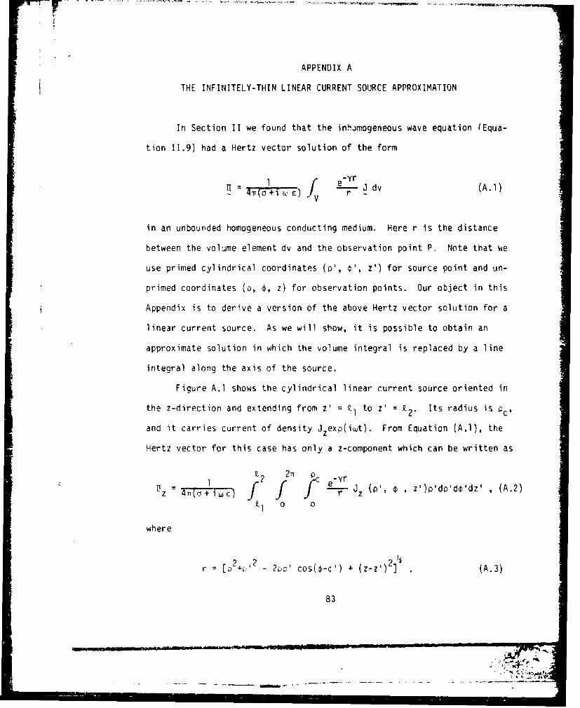
APPENDIX A

THE INFINITELY-THIN LINEAR CURRENT SOURCE APPROXIMATION

In Section II we found that the inhimogeneous wave equation (Equa-

tion 11.9) had a Hertz vector solution of the form

1 e Lyr J dv (A.l)

in an unbounded homogeneous conducting medium. Here r is the distance

between the volume element dv and the observation point P. Note that we

use primed cylindrical coordinates (P', "', z') for source point and un-

primed coordinates (o, €, z) for observation points. Our object in this

Appendix is to derive a version of the above Hertz vector solution for a

linear current source. As we will show, it is possible to obtain an

approximate solution in which the volume integral is replaced by a line

integral along the axis of the source.

Figure A.l shows the cylindrical linear current source oriented in

the z-direction and extending from z' = Zl to z' = 12" Its radius is Qc-

and it carries current of density Jzexp(iwt). From Equation (A.l), the

Hertz vector for this case has only a z-component which can be written as

F I Z 2 /T+ p 1 e-yr Jz (p, z')p'dQ'ddz' , (A.2)z ~ ~ • 4n (o+ow f

where

2 22r [o +f,' 2-p? cos(€-¢') + (z-z') (A.3)

83

-.6

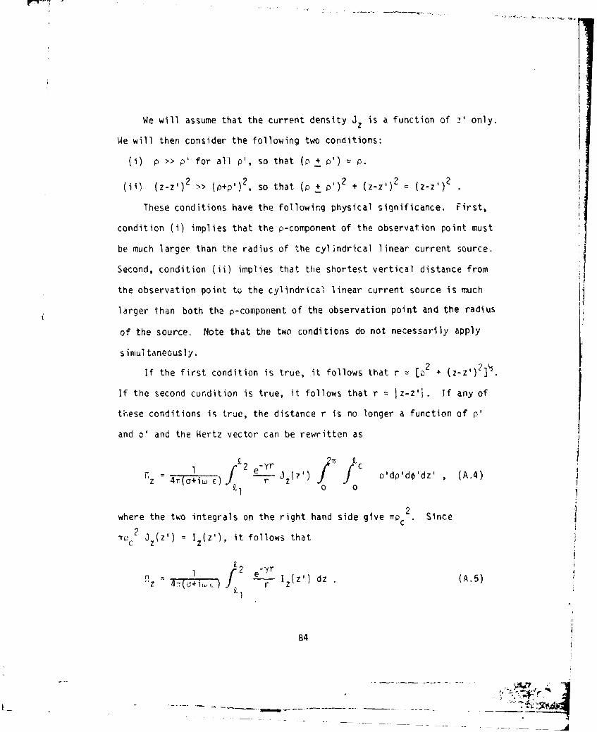
We will assume that the current density JQ is a function of z' only.

We will then consider the following two conditions:

(i) p > p' for all p, so that (p + p') v p.

(ii) (z-z,)2 > ' ,2 so that (p + p,)2 + (z-z')2 = (z-z') 2

These conditions have the following physical significance. First,

condition (i) implies that the p-component of the observation point must

be much larger than the radius of the cylindrical linear current source.

Second, condition (ii) implies that the shortest vertical distance from

the observation point tQ the cylindrical linear current source is much

larger than both the p-component of the observation point and the radius

of the source. Note that the two conditions do not necessarily apply

s imull taneous I y.If the first condition is true, it follows that r = [ 2 + (z-z,) 2 P½.

If the second cundition is true, it follows that r = jz-z'l. If any of

these conditions is true, the distance r is no longer a function of p'

and 0' and the Hertz vector can be rewritten as

•2 e- '' /yr ic

z = ______ eE f(r jZ f o'dp'd,'dz' , (A.4)ZI0 0

2where the two integrals on the right hand side give np c Since

'n2 j (Z') = I (z'), it follows that•C ' z

/2 rE • l _2 'r I z z ) dz (A.5)

84

~J7A

Ir

z

r ft~z ~ dvj

+ - B

III

Figure A.I. Cylindrical antenna of finite length (9,2 - ZI) and finitecross-section (radius ,)c) carrying a current with a uniform densityJz. A small volume element dv of the antenna is also shown in thefigure.

85

In our derivations, we have always used Equation (A.5) for the Hertz

vector. This means that all our field expressions are valid as long as

one of the above conditions (i) and (ii) are satisfied, i.e., as long as

the shortest distance from the observation point to the cylindrical

linear current source is much larger than the radius of the cylindrical

linear current source itself. In other words, we assume that the linear

current source is infinitely thin.

t86

86j

*B a= T . . .. . . .. i , , li i I I i •I I i i i! i

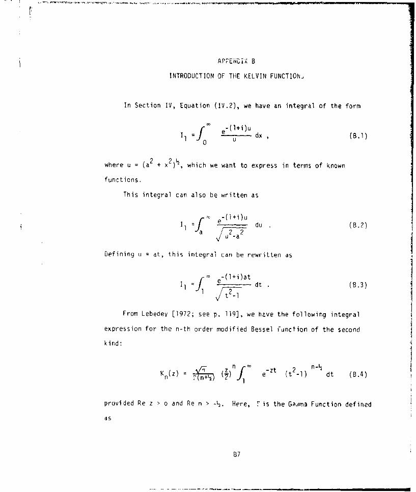
APPENDI1X B

INTRODUCTION OF THE KELVIN FUNCTION,

In Section IV, Equation (IV.2), we have an integral of the form

Ifo e -(l+i)uf e dx (B.1)

0 U

2 2½where u = (a + x2) , which we want to express in terms of known

functions.

This integral can also be written as

•a e-(l+i)u d B?Il = e du (B.2)

u -a

Defining u at, this integral can be rewritten as

e -(l+i)atI1 Jl 2e dt (8.3)

t 1

From Lebedev [1972; see p. 119], we have the following integral

expression for the n-th order modified Bessel function of the second

kind:

_n zn-t n-½Kn (Z) : () et (t ) dt (B.4)

1

provided Re z > o and Re n > -½. Here, r is the Gampma Function defined

as

87

r (n) = yn'le-Ydy. (B.5)

0

Choosing n 0 and knowing that P (½) V- , Equation (B.4) becomes

r -ztK0(z) e - dt. (B.6)

"1l t2l

Substituting z = a(l+i) in Equation (B.6) and comparing it with Equation

(B.3), we obtain

Ko (a(lI+i)) = .1B7

in other words, the integral I1 is a zero-th order modified Bessel func-

tion of the secoid kind of complex argument. Knowing this fact, we

can now proceed to write I1 in terms of known functions.

Since y = (l+i)ý and a = ., we have

K ( a(l+i) ) = Ko(yo) (B.8)

and from these relations it follows that

K1 h ('•Ž) : e dx. (B.9)0 f u

0

We also know from Dwight (1961] that

83

VB

n Kn - kern a + i kein X , (B.10)

where kern a and kein a are Kelvin functions of the second k..d of order

n [Young and Kirk, 1964]. The left hand side of Equation (B.10) can

also be written as

K n 31 ý i -)= K n ( O.(,!+i>/F/2- (B.11)

Letting n = 0 and following equations (B.8) - (B.11), we have

,-= K06,0) kero0 (2a) + i kei, (Ta) a (.12)

We have now expressed the integral II in terms of known Kelvin

functions. If we decompose II in equation (8.9) into its real and

imaginary parts, we obtain

I Ko(yl) *,f eUcos U dx -i e-Usin u dx , (B.13)0 0

then, comparing equations (B.12) and (B.13), it follows that

ker 0 ( F2a) f e Uýos u dxU

0

(B.14)

keio (J2 a) esnudx

0

89

- - i

If we let the upper limits of the integrals given by Equation (111.8)

go to infinity and compare the results with the integrals in Equation

(B.14), we can write

kero ( a) j dx - E [a ,

0(B.15)

kei 0 (•2-a) = - Es [a, c]

Similarly, if we also let the upper limits of the integrals given

by Equation (111.16) go to infinity and compare the results with the

derivatives of the Kelvin functions given by Equation (B.14), we obtain

ker' (F2-a) - ( Mc~a' •] + m1s[a, o0] + Nc[a, •] )(B.16)

kei' ( F2a) = _ Mc[a, M- La, -)

Since we also know that

ker, (j'a) = 1 ker ( F2 a) - keio (4 2 a))

(B.17)

kei1 Q2a) = (ker0 (F2-a) + kei0 (.2-a))

we can substitute Equations (B.16) into Equations (8.17) and obtain

ker1 (F2a) =-. ( 2M, [a, 4o) * Nc [a, +] + Ns [a,

(B.18)keiI (•-a) -- akei1 (F2a) = 2Mc [a, c] + Nc [a, c] - Ns [a,

90

APPENDIX C

FIELDS PRODUCED BY A DC CURRENT

In this appendix we summarize the electric and magnetic field

expressions for dc currents flowing in linear current sources of

infinitesimal, finite, semi-infinite, and infinite length.

1. Current Element Source

The fields produced by linear current element of length di and

carrying a dc current I are given by

31d. sine cose

Ez dZ9r3 (3 cos 2e -6 ) , (C.l)

H .Id" sine247T r

and

Eý =H = Hz = 0.

2. Linear Current Source of Finite Len th

The fields due to a linear current source of finite length carrying

a dc current I and extending from ZI to z2 are

9i

L,•••-I I II '

=ý 4Tra] ý-

Ez I z-Z2 z Zi• r

- o - 3 (C.2)42, r^3

andH b I z-91 z-•22

4-a p r 1 r 2

with E Hi Hz 0S P

Now consider a perpendicular line passing through the center of the

source. Along this line, E = 0 and we haveP

Ez_-IL

4-or

and

- IL

41Tor

where L = -2 kl is the length of the source.

If we normalize all the distances to the length L of the source,

we obtain

LE = -Iz 4 T r c rL 3

and (C.3)

LH 4 7 1r

where PL p/L and rL = r/L.

92

q -Arm-

In Figure C.1, we have plotted the variation of the magnitude of

the normalized Ez field (i.e., E zL 2 ) with normalized distance p

3. Linear Current Source of Infinite Length

Given a linear current source of infinite length carrying a dc

current I, all the field components are zero except for the magnetic

field component H., where

H 2--- (C.4)ýP 2 T-.

4. Linear Current Source of Semi-Infinite Length

In the case of a semi-infinite linear current source extending from

_o to 9,2 and carrying a dc current I, we have

E 01

Z (z-Z 2 ) (C.5)

2 -2

and

E HO Hz = 0

5. Linear Current Source of Infinite Length with a Finite Gap

Assuming the direction of current flc,"' ir the same in the two

segments of the source (Figure VI.l(d)), we have

93

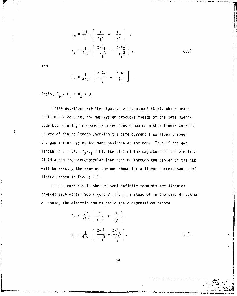
E0 PIEz 4- rl 3 (C.6)

and

H• • 2 r1

Again, E, H = H = 0.

These equations are the negative of Equations (C.2), which means

that in the dc case, the gap system produces fields of the same magni-

tude but pointing in opposite directions compared with a linear current

source of finite length carrying the same current I as flows through

the gap and occupying the same position as the gap. Thus if the gap

length is L (i.e., - L), the plot of the magnitude of the electric

field along the perpendicular line passing through the center of the gap

will be exactly the same as the one shown for a linear current source of

finite length in Figure C.l.

If the currents in the two semi-infinite segments are directed

towards each other (See Figure VI.l(b)), instead of in the same direction

as above, the electric and magnetic field expressions become

•._I 1_÷_ _ _

4E T 7 4 r r3 r 3 '

Ez I + (C.7)'9 2

94

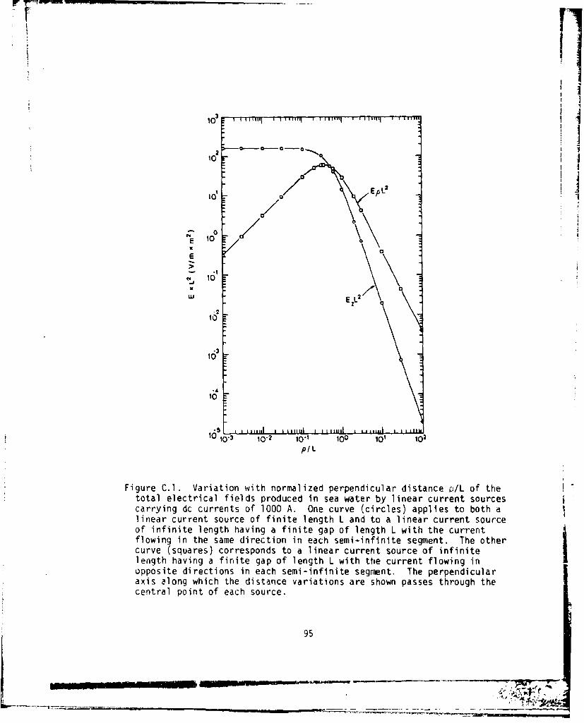
10 iii 1111" 1 I-• ,. I 11 1111 ii' I IIl] • 1 i ii

0 0-0

2pL2

10

0E 10

E L2w E~z,

-210

1.3

10

16 510-5U v v ivid a a q il a a ,im l 1,,,,.1 1 1v I [10-2 10-1 100 101 102

pIL

Figure C.l. Variation with normalized perpendicular distance Q/L of thetotal electrical fields produced in sea water by linear current sourcescarrying dc currents of 1000 A. One curve (circles) applies to both alinear current source of finite length L and to a linear current sourceof infinite length having a finite gap of length L with the currentflowing in the same direction in each semi-infinite segment. The othercurve (squares) corresponds to a linear current source of infinitelength having a finite gap of length L with the current flowing inopposite directions in each semi-infinite segment. The perpendicularaxis along which the distance variations are shown passes through thecentral point of each source.

95

miss*.

and

_i [ Z-Zl z-Z 2

If we now restrict ourselves to the fields produced along the

perpendicular line passing through the center of the gap of finite

length L and normalize all the distances with L, we obtain

IL2E= - _L_

L 22E rjL

E = , (C.8)

H= 0

The variation of the magnitude of the normalized E, field (i.e., E L2 )

with normalized distance OL for this case is plotted in Figure C.1.

If we now compare the electric field variations shown in

Figure C.I. we find that the electric field produced by the gap system

with opposite current flow shown in Figure VI.l(b) declines less rapidly

with distance (once • exceeds L/2) than the electric field produced

eitner by the gap system with currents flowing in the same direction in

each semi-infinite segment, as shown in Figure VI.l(a), or by the linear

current source of length L. The respective slopes of the two curves are

-20 dB/decade and -30 dB/decade at large distance.

96

I - r

APPENDIX D

FIELDS PRODUCED BY ARRAYS OF LONG CABLES SUBMERGED

IN A CONDUCTING MEDIUM OF INFINITE EXTENT

As discussed in Chapter VIII, the data displayed in the figures in

Chapter IV suggest that a single submerged cable cannot produce electric

or magnetic yields with the right frequency/amplitude characteristics

for successful undersea communication once the range exceeds some value

that will typically lie in the range 1 - 10 km (the actual value will

depend on a number of practical details; some of the most important of

these details are the frequency, the amplitude of the current in the

cable, the amplitude of the signal, the range, the background noise

level, and the sensitivity of the receivers). However, there appears to

he no reason why the range cannot be extended more or less indefinitely,

in principle, by the use of arrays of long cables. The problem of range

is then converted to a problem of cost and of power availability. in

this appendix we briefly consider some of the requirements for these

arrays and the ranges that might be achieved.

As a first example of an array of long cables, consider the config-

uration of cables (length L) shown in the top panel of Figure D.l. We

will refer to this confiquration as a series array, and we will assume

that L is so large that we can treat each cable in the array as a linear

current source of infinite extent and thus compute the electric and mag-

netic fields they produce from the expressions and data given in Chapter

IV. We also assume that the spacing s, although small compared with L,

is large enough for each cable to be treated as being independent of its

97

1z-1

neighbors. A second example of an array of long cables, a parallel

array, is shown in the bottom panel of Figure D.1; we will make the same

assumptions for this array as those we have just detailed for the series

array. We will suppose that the origin of a 3-dimensional cartesian

coordinate system (x,yz) is located at the center of each array and

that the planes of the two arrays correspond to the x,y planes of the

coordinate systems, with the y axis taken parallel to the cables as

shown in the figure.

Cross-sections of the two arrays, taken along the x-axis in Figure

D.1, are shown in Figure D.2. Here the cables are designated Cn, Cn+12

... C1l, C~l .. Cn according to their position relative to the origin

of the coordinate system. Considering the series array first, it is

easily seen that the total electric field at an obbervation point loca-

ted at a height h above the origin, i.e., at the point (0,O,h) is always

zero. However, the magnetic fields produced by each cable add up vec-

torially and give a total magnetic field that is directed along the 7-

axis. The first two vector contributions to this field, the magnetic

fields B+l and B-1 produced by the two nearest cables, are shown in the

figure. The electric and magnetic fields produced by the parallel array

differ substantially from those produced by the series array. Consider-

ing the fields produced at the point (0,0,h) once again, we find that the

parallel array does produce an electric field, unlike the series array,

and the field is directed along the y axis. Further, instead of being

directed along the z-axis, i.e., in a direction perpendicular to the

plane of the array, the magnetic field produced by the parallel array is

98

YI' I

L (a)

, ,I I

I I

2n1

I

2n1

Figure 1).. Two different arrays of parallel long cables (length L,spacing = s; s<-L) lying in the same plane and all carrying the samecurrent I. In the top panel (a) we show a series array, where thecurrent in a particular cable flows in the opposite direction to thecurrent in the adjacent cables. In the bottom panel (b) we show aparallel array, where the current in all the cables flows in thesame direction. Note that the total current flowing through theseries array is I, whe,-eas the total current flowing througn theparallel array is 2n0, where 2n (n = 1,2,3...) is the number of cablesin each array.

99

r

directed along the x-axis, i.e., in a direction parallel to the plane of

the array. These various properties of the fields do not apply general-

ly, but they illustrate the large differences that can occur in the

fields produced by the two arrays.

In considering arrays, our primary interest is to produce measurable

electric and/or magnetic fields throughout as large a volume of the sea

as possible, with the least number of cables. Cr, since the sea is com-

paratively limited in dep.n compared with horizontal extent, we wish to

produce measurable fields throughout the sea over as large an area as

possible. Clearly the cables in the arrays (which we now assume are lo-

cated on the sea floor, aiLnouah 'is is not a necessary condition for

the use of the a-rays we have been considering) must be spaced far apart,

with the actual spacing being determined by the fields produced at points

midway between the cables, where the attenuation of the fields is rela-

tively the strongest and where the field amplitudes are in most cases a

ninimum for a given height h above the plane of the arrays. To illus-

trate the amplitudes of the fields that can be produced, we have taken

the series array shown in Figure D.l(a) and D.?(a) and computed the vari-

ation of the amplitude of the total magnetic field with height h along

two axes perpendicular to the plane of the array: the z-axis, which

passes through a point (the origin) located midway between two cables,

and an axis passing throuýgh one of the cables. Because our interest is

in tl fields produced by an array of widely spaced cables, we assume

that the distance s between the cables is 30 skin depths, which means

that we can reasonably neglect the fields produced along our two chosen

100

7Lpr

"-" v "-2

C .2 c., C., C .2

(a)

8,

C.2 C.aC C.2

s- s 4---,2; -- s

(b)

Figure D.2. Cross-sectional views of the two arrays of long cablesshown in Figire D.l. At top is the series array, where the directionof the current in any cable is opposite to the direction of the currentin adjacent cables; at bottom is the parallel array, where the direc-tion of the current is the same in all cables. The magnetic fieldsB-1 and B+l produced at the observation point (o.o,h) by the two cablesC-1 and C+l are shown for each array.

101

.. =

axes by all the cables in the array except for the one or two cables

nearest to the axes. Equation (IV.6) is used to obtain the magnetic fields

produced by these cables.

Figure D.3 shows the results of the computations. The data are

presented in parametric form, so that they apply at any ULF/ELF frequency,

and it is immediately apparent by comparing the two curves in the figure

that the total magnetic field produced along the axis passing through

one of the cables is very much greater than the field produced on the

axis passing through a point midway between two of the cables. Using

the results for the latter axis and assuming that the minimum value of

the magnetic field that can be measured is 10 1 pT, we find that for a

100 Hz, 1000 A current in the cables the magnetic field can be measured

up to h = 200 m away from the array, and for 1 Hz, 1000 A current in the

cables the magnetic field can be measured up to h I km away from the

array.

The above field strength considerations are perhaps the most impor-

tant in evaluating the possible undersea communication performance of

cable array. However, there are a few other considerations that are

also important, which we list before concluding this appendix. First,

because communication is to take place from the bottom upwards in the

sea, it may not be necessary for measurable electric or magnetic fields

to be produced at the surface. Second, because most and perhaps all

natural ULF/ELF noise in the sea comes from sources above the surface,

the signal-to-noise ratio for communications via undersea cable arrays

should increase with depth. Further, because the electric and magnetic

102

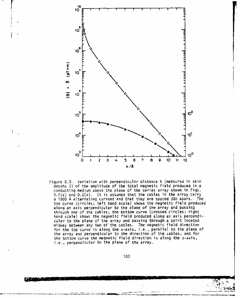
1010

10

10 0

0

21010

-. \

10 1 2- \o\

10 4 101

0 1 2 3 4 5 6 7 8 9 10 11 12

h/B

Figure 0.3. Variation with perpendicular distance h (measured in skindepths 6) of the amplitude of the total magnetic field produced in aconducting medium above the plane of the series array shown in Figs. ID.l(a) and D.2(a). It is assumed that the cables in the array carrya 1000 A alternating current and that they are spaced 306 apart. Thetop curve (circles; left hand scale) shows the magnetic field producedalong an axis perpendicular to the plane of the array and passingthrough one of the cables; the bottom curve (crossed circles; righthand scale) shows the magnetic field produced along an axis perpendi-cular to the plane of the array and passing through a point locatedmidway between any two of the cables. The magnetic field directionfor the top curve is along the x-axis, i.e., parallel to the plane ofthe array and perpendicular to the direction of the cables, and forthe bottom curve the magnetic field direction is along the z-axis,i.e., perpendicular to the plane of the array.

103

' - .' • .:

fields from these natural sources are predominantly horizontally directed

in the sea, it may be possible to discriminate against the natural noise

by generating and measuring vertically-directed fields in the sea.

104

• -, . f•: .•.

I

DISTRIBUTION LIST

No. of No. ofOrganization Copies Organization Copies

Director Naval Research LaboratoryDefense Advanced Research Information Technology Division

Projects Agency ATTN: J. R. Davis 1ATTN: Program Management 2 4555 Overlook Avenue, SW

TTO, R. A. Gustafson 1 Washington, D.C. 20375TTO, P. A. Selwyn 1

1400 Wilson Boulevard Naval Ocean Systems CenterArlington, VA 22209 ATTN: Library 1

W. Moler 1Defense Technical C. F. Ramstedt 1

Information Center 12 Y. Richter 1Cameron Station K. L. Grauer 1Alexandria, VA 22314 271 Catalina 5oulevard

San Diego, CA 95152Office of Naval ResearchATTN: Code 414 1 Naval Electronic Systems

Code 222 1 CommandCode 425 1 ATTN: PME-l10-112

800 North Quincy Street PME-110-XI 1Arlington, VA 22217 Department of the Navy

Washington, D.C. 20360Office of Naval ResearchResident Representative 1 Naval Underwater Systems CenterUniversity of California, New London Laboratory

San Diego ATTN: P. BannisterLa Jolla, CA 92093 A. Bruno

J. Orr 1Office of Naval Research E. Soderberg 1Resident Representative 1 New London, CT 06320Stanford UniversityRoom 165 - Durand Building Naval Surface Weapons CenterStanford, CA 94305 White Oak Laboratory

ATTN: J. J. Holmes 1Deputy Assistant Secretary M. B. Kraichman 1

of Defense P. WesselDefense Research anS Silver Spring, MD 20910

Engineering for CATTN: T. P. Quinn 1 David W. Taylor Naval ShipPentagon Research and DevelopmentWashington, D.C. 20301 Center

ATTN: W. Andahazy 1Office of Assistant Secretary F. E. Baker 1

of the Navy (R, E&S) P. Field 1ATTN: J. Hull 1 Annapolis, MD 21402Pentagon, Room 5E 779Washington, D.C. 20350

, . ,

DISTRIBUTION LIST (Continued)

No. of No. ofOrganization Copies Organization Copies

Naval Ocean R&D Activity Science Application, Inc.ATTN: D. L. Durham 1 ATTN: J. Czika, Jr.

D. W. Handschumacher 1 1710 Goodridge DriveK. Smits 1 McLean, VA 22102

NSTL StationBay St. Louis, MS 39522 Director

Defense Nuclear AgencyNaval Oceanographic Office ATGTN: RAAE 2ATTN: 0. E. Avery 1 DDST I

T. Davis 1 RAEV 2G. R. Lorentzen 1 Washington, D. C. 20305

NSTL StationBay St. Louis, MS 39522 R&D Associates

ATTN: C. GreifingerNaval Air Systems Command P. 0. Box 9695ATTN: B. L. Dillon 1 Marind del Rey, CA 90291Washington, D.C. 20361

Pacific-Sierra Research Corp.Naval Intelligence ATTN: E. C. Field

Support Center 1456 Cloverfield BoulevardATTN: G. D. Batts 1 Santa Monica, CA 904044301 Suitland RoadWashington, D.C. 20390 Johns Hopkins University

Applied Physics LaboratoryNaval Postgraduate School ATTN: L. W. Hart 1Department of Physics and H. Ko I

Chemistry Johns Hopkins RoadATTN: 0. Heinz 1 Laurel, MD 20810

P. Moose IMonterey, CA 93940 University of California

Scripps Institute ofNaval Coastal Systems Center OceanographyATTN: R. H. Clark 1 ATTN: C. S. Cox, Code A-030

M. J. Wynn 1 La Jolla, CA 92093Panama City, FL 32407

Lockheed Palo Alto ResearchSRI International LaboratoryATTN: D. M. Bubenik 1 ATTN: W. Imhof I

J. B. Chown 1 R. G. JohnsonR. C. Honey 1 J. B. Reagan

333 Ravenswood Avenue M. Walt 1Menlo Park, CA 94025 3521 Hanover Street

Palo Alto, CA

DISTRIBUTION LIST (Continued)

No. of No. ofOrganization Copies Organization Copies

La Jolla Institute ChiefATTN: K. Watson 1 Air Force TechnicalLa Jolla, CA 92407 Applications Center 1

HQUSAFUniversity of Texas, Austin Patrick AFB, FL 32925Geomagnetics and Electrical

Geoscience Laboratory CommanderATTN: F. X. Bostick, Jr. 1 Air Force Systems Command 2Austin, TX 78-12 Andrews AFB, MD 20331

EG & G CommanderATTN: L. E. Pitts 1 Air Force Geophysics LabP. 0. Box 398 ATTN: Technical Library 1Riverdale, MD 20840 Hanscom AFB, MA 01731

3

a.' -- -

• •'• • '-•" • •-T•"- •~ .9'-" . . ' •'m l 7