Radio Planning and Management of Energy-Efficient Wireless ... · RADIO PLANNING AND MANAGEMENT OF...

POLITECNICO DI MILANO

RADIO PLANNING AND MANAGEMENT OF ENERGY-EFFICIENT WIRELESS

ACCESS NETWORKS

SILVIA BOIARDI

DIPARTIMENTO DI ELETTRONICA, INFORMAZIONE E BIOINGEGNERIA


Thesis director: Prof. Antonio Capone

Thesis co-director: Prof. Brunilde Sanso

Tutor: Prof. Michele D’Amico

PhD coordinator: Prof. Carlo Ettore Fiorini

THESIS PRESENTED TO OBTAIN THE DIPLOMA OF

PHILOSOPHIÆ DOCTOR

(INFORMATION TECHNOLOGY, CYCLE XXVI)

JULY 2014

c© Silvia Boiardi, 2014.


This thesis titled:

RADIO PLANNING AND MANAGEMENT OF ENERGY-EFFICIENT WIRELESS

ACCESS NETWORKS

presented by: BOIARDI Silvia

to obtain the diploma of: Philosophiæ Doctor

has been accepted by the examination board consisting of:

Mr GIRARD Andre, Ph.D., president

Mrs SANSO Brunilde, Ph.D., member and research director

Mr CAPONE Antonio, Ph.D., member and research co-director

Mrs CARELLO Giuliana, Ph.D., member

Mrs MEO Michela, Ph.D., member

iii

DEDICATION

To my family,

faraway. . . so close

iv

ACKNOWLEDGEMENTS

The completion of my doctorate dissertation has been a wonderful and often overwhelming

journey. I could not say whether it has been grappling with the topic itself which has been the

real learning experience, or grappling with how to write papers, give presentations and deal

with deadlines... In any case, it is a pleasure to express my thanks to those who contributed

in many ways to the success of this study and made it an unforgettable experience.

I would like to give the first, heartfelt thanks to my supervisor at Ecole Polytechnique

de Montreal Prof. Brunilde Sanso, woman of admirable strength and determination. This

work would not have been possible without her guidance and support. She has oriented me,

giving me valuable advices on research-related as well as more personal matters. She has

kept me on track during the hardest moments of my doctorate, pushing me to give my best

in every circumstance. She has been demanding, tough on me when she needed to be; at

the same time, she has been patient, encouraging and caring, always available to listen and

discuss new ideas or compelling issues. Her ability to approach problems, her intuition and

her way of thinking set an example for me. Working with her has been a real pleasure, and

I am honored to become her first female Ph.D. graduate.

I am also deeply grateful to my supervisor at Politecnico di Milano Prof. Antonio Capone.

In spite of his being the busiest man I know, and regardless of the distance that separated

us for most of the doctorate duration, he has always found the time to closely follow the

development of my research. His wide expertise has been invaluable to the completion of

my dissertation. He has always had an answer to my many questions, or a kind word when

I needed to be reassured. When I got too serious, his humor and friendliness have helped

me laugh and lightened my perspective. Most of all, he believed in me and offered me the

opportunity to grow and become what I am now.

I am very thankful to the remaining members of my dissertation committee Prof. Andre

Girard, Prof. Michela Meo and Prof. Giuliana Carello, as well as to my tutor at Politecnico

di Milano Prof. Michele D’Amico, for their suggestions and remarks on my doctoral thesis as

well as for their academic support. In particular, I would like to thank Prof. Andre Girard

for his insightful comments and precious help on some challenging parts of my research work.

I will never forget the big help that came from the personnel of Ecole Polytechnique de

Montreal and Politecnico di Milano. My sincere gratitude goes to Nathalie Levesque, Nadia

Prada and Samara Moretti, who drove me through the bureaucratic and academic require-

ments of both institutions. Many thanks to the personnel of GERAD, and in particular to

Marie Perrault, Francine Benoıt, Carol Dufour and Marilyne Lavoie. These ladies’ heart-

v

warming smile, not to mention their willingness and commitment to their job, is what really

runs the research group. Thanks also to Pierre Girard and Christophe Tribes, who patiently

answered my questions and solved my problems regarding computers and programming.

On the road to my Ph.D., I was very lucky to have crossed paths with some brilliant minds

and great people who became friends over the last years. I owe a great deal of gratitude to

Ilario, who has been a valuable advisor and a fun traveling companion. No matter how

much work he had to do, he has always carved out some time to discuss with me about

research issues or ideas. Thanks to Luca, who lived this “double doctorate adventure” with

me, for his enthusiasm and pragmatism. His passion for the research have motivated me to

always work to the best of my abilities. Also, I could not have completed all the required

paperwork and delivered it to the correct place without his reminders. Thanks to Filippo

and Eleonora for their support and for the good times together, and to Carmelo, Federico,

Arash, Marni and Hadami, for sharing their knowledge with me and providing a pleasant and

productive working atmosphere. Thanks to my coffee break buddies Marco Paolo, Alessandro,

Laura, Lorenzo and Marco, for making my days at Politecnico di Milano way more fun and

stimulating.

A special thanks goes to my life-long friend Rossella, for her unconditional moral support

and encouragement, and to Marco and Chris, for their jokes and sense of humor that have

always kept me smiling. I would also like to thank my dear friends Francesca and Stefania,

who have never stopped asking me about the progress of my research work.

Of course, no acknowledgments would be complete without giving thanks to my parents.

They have taught me about hard work and self-respect, about persistence and about how

to be independent. They have hidden their sadness when their only child flew the nest to

live this life changing experience, but they have always shown how proud they are of me and

what I have become. I am proud of them too, and grateful for them and for the“smart genes”

they passed on to me.

Finally, “thank you” is not quite enough to express how grateful I am to Trevor, who has

held my hand throughout the happiest and the toughest moments of this doctorate. Together

we cheered and cried, laughed and argued, had fun and worked hard, discussed about the

present and planned our future. It is only through his love and unwavering belief in me that i

could complete my dissertation, because a journey is easier when you travel together. Trevor

taught me the most important lesson that I have learnt during these years: to achieve what

you have waited so long for, you have to stay strong, keep your head up and be patient.

There is always a reward in all hard-work and sacrifice.

vi

SOMMARIO

Nel ultimi anni, grazie alla continua offerta di prodotti e servizi innovativi divenuti par-

te integrante della nostra quotidianita, il settore delle tecnologie dell’informazione e delle

comunicazioni (information and communication technology, ICT) ha assunto un ruolo fon-

damentale nello sviluppo economico. La continua crescita e diffusione delle ICT non ha solo

trasformato il nostro stile di vita, ma anche attirato l’attenzione sull’impatto delle tecnolo-

gie dell’informazione e comunicazione sul problema del surriscaldamento globale. In questo

contesto di accresciuta consapevolezza e nato il concetto di Green ICT, che ha come scopo la

ricerca di tecnologie e soluzioni eco-sostenibili ed energeticamente efficienti. Come parte fon-

damentale delle ICT, anche le reti di telecomunicazioni sperimentano una costante crescita ed

espansione. I vincoli di capacita e qualita del servizio offerto sono tra i maggiori responsabili

dell’aumento del consumo di energia delle reti. Per quanto riguarda le reti senza fili in parti-

colare, gran parte delle spese sostenute dagli operatori e dovuta alle alte esigenze energetiche

delle stazioni di base, considerate tra le componenti di rete con il piu alto assorbimento di

potenza.

Fino ad oggi, l’industria delle comunicazioni senza fili si e concentrata essenzialmente

sulla produzione di terminali mobili a basso consumo energetico al fine di attirare un maggior

numero di clienti e, di conseguenza, aumentare i profitti degli operatori di rete. D’altra parte,

negli ambienti di ricerca, la questione dell’efficienza energetica e affrontata da un punto di

vista piu ampio. Oltre allo sviluppo di dispositivi e protocolli ad alta efficienza energetica,

studi piu recenti riguardano la pianificazione e l’operazione energy-aware di reti wireless. I

problemi di design e gestione di reti green sono stati trattati sotto molteplici aspetti, ma

mai in maniera congiunta, trascurando il fatto che l’efficacia di un’operazione di rete a basso

consumo energetico dipende strettamente dalle decisioni prese in fase di pianificazione.

Il lavoro di ricerca presentato in questa tesi di dottorato mira a colmare questa lacuna

tramite lo sviluppo di un sistema di ottimizzazione che considera unitamente il design e

l’operazione delle reti senza fili. Il problema congiunto di pianificazione e gestione energetica

(joint planning and energy management problem, JPEM) proposto punta a dimostrare che,

quando il meccanismo di cell sleeping e utilizzato come tecnica di gestione di rete, il livello

di flessibilita offerto dalla topologia installata aumenta fortemente la capacita della rete

di adattarsi alle variazioni del traffico offerto. Minimizzando il trade-off tra gli investimenti

iniziali (capital expenditures, CapEx) dovuti all’installazione delle stazioni di base, e le spese di

operazione e gestione (operational and management expenditures, OpEx), calcolate sulla vita

della rete, il modello stima la topologia a piu alta efficienza energetica ottenibile rispettando

vii

eventuali vincoli imposti dall’operatore di rete sulle spese di capitale.

In questo studio sono prese in analisi due tecnologie di rete d’accesso. Come intuibile dal

nome, il problema congiunto di pianificazione e gestione energetica per reti cellulari (joint

planning and energy management problem for cellular networks, JPEM-CN) e stato svilup-

pato per il design e la gestione dell’operazione di reti cellulari. Tre tipi di celle (macro, micro

e pico) possono essere utilizzate per la copertura di un’area dove non vi e alcuna stazione

d’accesso preesistente. La zona in esame e caratterizzata da un profilo di traffico giornaliero

realistico; di conseguenza, il traffico offerto dai punti di concentrazione (test points, TPs)

distribuiti in maniera aleatoria nell’area viaria a seconda del periodo di tempo considerato.

I risultati numerici ottenuti testando sei scenari differenti mostrano che, al costo di un leg-

gero aumento in CapEx, una rete pianificata per essere energicamente efficiente permette di

risparmiare circa il 50%–60% rispetto all’energia necessaria all’operazione della topologia di

costo minimo. Dai risultati appare inoltre che, mentre le reti a costo minimo sono composte

prevalentemente da celle di grandi e medie dimensioni, le topologie ad alta efficienza ener-

getica comprendono alcune macro celle a supporto di numerose micro e pico celle, le quali

possono essere spente facilmente durante i periodi di minor traffico senza violare i vincoli di

copertura totale.

Un altro sistema di ottimizzazione e stato modellizzato per risolvere il problema congiunto

di pianificazione e gestione energetica per reti a maglie senza fili (joint planning and energy

management problem for wireless mesh networks, JPEM-WMN ). In questo caso, due tipi

di stazioni d’accesso possono essere installate nella zona considerata: routers, in grado di

connettersi ad altri dispositivi di rete, e gateways, che offrono anche un accesso diretto ad

Internet. La domanda degli utenti situati nell’area varia a seconda di un profilo di traffico

definito; inoltre, due gradi di congestione sono presi in esame, standard ed elevato. Il modello

proposto e stato testato su sei scenari. Nonostante gli stessi vantaggi osservati per JPEM-CN

si possano riscontrare nel caso delle reti a maglia, il risparmio energetico risulta minore a causa

della scarsa flessibilita delle reti magliate in confronto a quella di reti cellulari eterogenee.

Con piccoli incrementi delle spese di capitale, il modello JPEM-WMN permette comunque

una riduzione del consumo di energia del 25–30% nella maggior parte dei casi.

In questa tesi son esaminate alcune varianti dei due modelli di JPEM. Uno degli obiettivi

del lavoro di ricerca e quello di valutare l’impatto di un sistema di modellizzazione congiunto

rispetto ad un approccio piu tradizionale in cui l’ottimizzazione delle spese di capitale e

affrontata in un prima fase, seguita dalla gestione dell’operazione della rete installata. E

stato quindi sviluppato un approccio in due fasi (two-step), in cui la rete di costo minimo e

prima installata e successivamente gestita. I risparmi energetici misurati sono stati utilizzati

per valutare la riduzione del consumo d’energia ottenuto tramite i modelli JPEM per reti

viii

cellulari e a maglia.

Un’altra importante variazione, formulata per entrambe le tecnologie di accesso, consiste

nel rilassare i vincoli di copertura globale al fine di garantire il servizio di rete soltanto per

gli utenti attivi. In questo modo, le stazioni di base che coprono solo utenti inattivi possono

essere spente, con l’effetto di diminuire ulteriormente la consumazione energetica della rete. I

test condotti sugli scenari di rete cellulare dimostrano che, quando si considera una copertura

di rete dei soli clienti attivi, e possibile ottenere un risparmio energetico supplementare del

25%–35%, mentre la percentuale e di circa 12% nel caso di reti magliate.

Per quanto concerne unicamente le reti cellulari, questa tesi comprende una variante del

problema JPEM-CN in cui il sistema non e libero di scegliere la topologia migliore (e quindi,

gli investimenti di capitale) a seconda dell’importanza dei costi energetici nella pianificazione

di rete. Al contrario, un parametro di budget e introdotto allo scopo di limitare i CapEx ad

un dato valore. Il modello Budget JPEM-CN ottiene risultati simili alla versione originale;

tuttavia, i nuovi vincoli sui costi di installazione della rete sembrano aumentare la complessita

della formulazione.

Riguardo le reti magliate, il modello On/Off JPEM-WMN presentato in questa tesi vin-

cola i dispositivi d’accesso a cambiare il loro stato (da attivo a inattivo e vice versa) una

sola volta nel corso della giornata. Questa formulazione ha come effetto la diminuzione dello

spreco energetico durante la transizione di stato delle stazioni di base; tuttavia, il risparmio

di energia derivato dallo spegnimento delle celle superflue alla copertura di rete e inevitabil-

mente ridotto. Altre variazioni minori sono state testate sul problema JPEM-WMN, come

l’uso di una capacita variabile anziche fissa per i link della rete dorsale, o la simulazione del

comportamento di una rete cellulare tramite l’installazione di soli gateways per eliminare la

connettivita multi-hop tipica delle reti a maglia.

Al fine di ottenere piu rapidamente una soluzione al problema congiunto per reti cellulari

e permettere lo studio di scenari di test di piu grandi dimensioni, nel corso della ricerca di

dottorato e stato messo a punto un metodo euristico ad-hoc in cui i problemi di pianificazione

e gestione di rete sono affrontati separatamente, cosı come i diversi intervalli temporali in cui

e divisa la giornata. Partendo da una topologia completa, l’euristica trova il piu efficiente

pattern di attivazione delle stazioni di base in grado di soddisfare le esigenze di copertura

sia durante il periodo di massimo traffico, quando e necessario servire un alto volume di

traffico offerto, sia durante il periodo di minor traffico, quando un maggior numero di stazioni

d’accesso puo potenzialmente essere spento. Il pattern di attivazione risultante e considerato

come una topologia parziale e fornito in ingresso al modello JPEM-CN originale. La topologia

iniziale e quindi integrata per ottenere la miglior soluzione possibile valida per tutti i periodi

temporali. Testato sugli stessi scenari di rete cellulare, il metodo euristico ha prodotto

ix

risultati che si discostano di circa il 10% dal limite inferiore dei risultati di JPEM-CN; inoltre,

nuovi scenari di dimensioni realistiche sono stati risolti con successo in meno di 15 minuti

nella maggior parte dei casi.

Nel complesso, le diverse formulazioni di JPEM dimostrano che, quando la topologia di

rete e concepita per essere eco-sostenibile, e possibile raggiungere risparmi energetici molto

elevati al costo di un moderato aumento rispetto al minimo investimento di capitale. A questo

scopo, e necessario tenere in considerazione gli effetti della gestione di rete durante la fase

di pianificazione. I risultati illustrati e gli esempi numerici mostrano che la coesistenza nella

stessa topologia di dispositivi d’accesso di diverse dimensioni e fondamentale per assicurare

la flessibilita della rete e permettere l’adattamento della rete stessa alle variazioni di traffico

nello spazio e nel tempo.

x

ABSTRACT

In the last years, the information and communication technology (ICT) sector has trans-

formed the way we live. Consistently delivering innovative products and services, the ICT

assumed a primary role on economic development and productivity, becoming an integral part

of everyday life. However, due to their wide and constantly increasing diffusion, the effect

of information and communication technologies on global warming can no longer be ignored.

The concept of Green ICT has originated with the aim of building awareness of this, thus

boosting the research toward environmentally sustainable, energy-efficient technologies and

solutions. As an important part of the ICT, telecommunication networks are experiencing

a booming growth. Capacity issues and quality of service constraints are some of the main

concerns that contribute to raise the power consumption. In particular, a large portion of

the electricity bill results from the high power requirements of wireless base stations, which

have been proved to be the most energy-hungry network components.

Up to now, the mobile communication industry has focused mostly on the development

of power-efficient mobile terminals, so as to attract a higher number of customers and con-

sequently increase the operators’ profits; on the other hand, the research world has been

investigating energy efficiency from a wider point of view. Besides studies on power-efficient

devices and protocols, more recent works addressed the problem of energy-aware design and

operation in wired and wireless network infrastructures. Many aspects and challenges of

green network planning and management have been explored; nevertheless, the two problems

have never been linked and tackled at the same time, neglecting the fact that an effective

power-efficient network operation largely depends on the decisions taken in the design phase.

The research presented in this doctoral thesis aims at filling this gap by developing an

optimization framework that jointly considers the design and operation of wireless networks.

The proposed joint planning and energy management problem (JPEM) strives to prove that,

when cell sleeping is adopted as network management technique, the level of flexibility offered

by the installed topology strongly improves the system capability to adapt to the varying

traffic load. By minimizing the trade-off between capital expenditures (CapEx) related to

the network deployment and operational and management expenditures (OpEx) calculated

over the network lifetime, the model finds the most energy-efficient network topology while

meeting the capital investment limitations imposed by the mobile operator.

Two types of access network are analyzed in this work. As the name suggests, the joint

planning and energy management problem for cellular networks (JPEM-CN) was developed

to plan and manage the operation of cellular networks. Three cell sizes (macro, micro and

xi

pico) are allowed to be deployed in an area where no previous access devices are installed. A

realistic daily traffic profile is assumed to characterize the area; therefore, the traffic offered by

the test points randomly distributed in the area varies in each time period. Numerical results

obtained by testing six different scenarios demonstrate that, with modest CapEx increases, a

network planned to be energy efficient can reach power savings around 50%–60% compared to

the energy saved by managing the operation of the minimum cost deployment. Moreover, the

results give an interesting insight on the different topology compositions. While the minimum

CapEx network is mostly composed of big and medium size cells, energy-aware topologies

include a few larger cells in support of many small cells, which can be put to sleep during

low traffic periods without leaving parts of the area uncovered.

Besides JPEM-CN, another optimization framework has been modeled to solve the joint

design and operation problem on wireless mesh networks (JPEM-WMN). In this case, only

two types of access station can be placed in the area: routers, that can only connect to

other routers, and gateways, having direct access to the Internet. Once again, a realistic

traffic profile is considered, according to which the mesh clients vary their traffic requests;

also, two degrees of traffic congestion are examined, standard and busy. The joint framework

were tested on six scenarios. Even though the same benefits of the JPEM-CN apply to

mesh networks, smaller energy savings are registered due to the lower flexibility of WMNs

in comparison to heterogeneous cellular networks. However, the JPEM-WMN model yields

savings of 25% to 30% in most cases with low extra installation costs.

Additional model variants for both JPEM models are also presented in this research. Since

one of the objective of the work is to evaluate the impact of using a joint modeling framework

compared to a more traditional CapEx optimization and successive network management, a

two-step approach is developed where the minimum cost network is first installed and then

operated. The energy savings served to fairly evaluate the reduction of power consumption

achieved by the cellular and mesh versions of JPEM.

Another important variation, formulated for both types of access technology, consists in

relaxing the total area coverage constraints to guarantee network service only to the active

test points or mesh clients. This way, access devices having only idle users in their coverage

radius can be put to sleep, further decreasing the energy consumption: results showed that

supplemental power savings of 25%–35% can be reached in cellular test scenarios, while the

percentage is around 12% in case of mesh instances.

Referring now only to cellular networks, this thesis includes a JPEM-CN variant where

the framework is not free to select the best topology (and thus, capital investments) according

to the relative importance of the energy saving component in the network planning. Instead,

a budget parameter is imposed in order to limit the CapEx to a certain value. The Bud-

xii

get JPEM-CN achieves similar results to the original version; however, the new constraints

capping the capital costs seem to add complexity to the model formulation.

For what concerns mesh networks, an interesting On/Off JPEM-WMN framework is pre-

sented where the access devices can switch their state, from idle to active and vice versa, only

once per day, reducing the power wasted during state transitions but inevitably decreasing

the energy savings from sleeping cells. Further minor changes have been also tested on the

JPEM-WMN during the course of the doctoral research, as the introduction of variable back-

bone link capacity, compared to the fixed capacity in the original model, and the elimination

of the multi-hop connectivity characteristics in order to simulate the behavior of a cellular

network, by allowing only the installation of mesh gateways.

In order to simplify the solution of the JPEM-CN and enable the evaluation of test

scenarios closer to real-size, an ad-hoc heuristic method was developed where the planning

and operation problems, as well as the daily time intervals, are tackled separately. Starting

from a complete topology, the heuristic finds the most efficient activation pattern that satisfies

the coverage requirements for both the peak traffic periods, where high traffic volumes have

to be served, and the off-peak, where the opportunity to save energy by turning off some

access stations is the highest. The resulting activation pattern is considered as a new partial

topology, which is provided as input to the original JPEM-CN; the initial topology is then

enriched to obtain the best feasible solution for all time periods. For the same cellular

test scenarios, the heuristic showed results only about 2% to 13% far from the respective

JPEM-CN objective functions; on the other hand, new larger scenarios have been tested and

successfully solved in less than 15 minutes in most of the cases.

On the whole, the various JPEM formulations proved that higher energy savings can be

obtained when the network topology is designed to be power efficient at the cost of moderate

increases in capital costs. To do so, the effects of the network management have to be

taken into consideration during the network design stages. Moreover, numerical results and

examples showed how the coexistence of multiple sizes of access device in the same topology is

fundamental to provide the network with enough flexibility to adapt to the traffic variations

in time and space.

xiii

TABLE OF CONTENTS

DEDICATION . . . . . . . . . . . . . . . . . . . . . . . . . . . . . . . . . . . . . . . . iii

ACKNOWLEDGEMENTS . . . . . . . . . . . . . . . . . . . . . . . . . . . . . . . . . iv

SOMMARIO . . . . . . . . . . . . . . . . . . . . . . . . . . . . . . . . . . . . . . . . . vi

ABSTRACT . . . . . . . . . . . . . . . . . . . . . . . . . . . . . . . . . . . . . . . . . x

TABLE OF CONTENTS . . . . . . . . . . . . . . . . . . . . . . . . . . . . . . . . . . xiii

LIST OF TABLES . . . . . . . . . . . . . . . . . . . . . . . . . . . . . . . . . . . . . . xvi

LIST OF FIGURES . . . . . . . . . . . . . . . . . . . . . . . . . . . . . . . . . . . . .xviii

LIST OF ACRONYMS AND ABBREVIATIONS . . . . . . . . . . . . . . . . . . . . . xix

CHAPTER 1 INTRODUCTION . . . . . . . . . . . . . . . . . . . . . . . . . . . . . 1

1.1 Research Context . . . . . . . . . . . . . . . . . . . . . . . . . . . . . . . . . . 1

1.2 General Objectives and Original Contribution . . . . . . . . . . . . . . . . . . 3

1.3 Document Structure . . . . . . . . . . . . . . . . . . . . . . . . . . . . . . . . 5

CHAPTER 2 LITERATURE REVIEW . . . . . . . . . . . . . . . . . . . . . . . . . 8

2.1 Green Networking . . . . . . . . . . . . . . . . . . . . . . . . . . . . . . . . . . 8

2.2 Green Techniques for Cellular Networks . . . . . . . . . . . . . . . . . . . . . . 10

2.3 Green Techniques for Wireless Mesh Networks . . . . . . . . . . . . . . . . . . 13

CHAPTER 3 DEVELOPMENT OF THE DOCTORAL RESEARCH . . . . . . . . . 15

3.1 Motivation . . . . . . . . . . . . . . . . . . . . . . . . . . . . . . . . . . . . . . 15

3.2 Content and Relevance of the Presented Articles . . . . . . . . . . . . . . . . . 16

3.3 Additional Research Work . . . . . . . . . . . . . . . . . . . . . . . . . . . . . 18

CHAPTER 4 ARTICLE 1: PLANNING FOR ENERGY-AWARE WIRELESS NET-

WORKS . . . . . . . . . . . . . . . . . . . . . . . . . . . . . . . . . . . . . . . . . . 21

4.1 Abstract . . . . . . . . . . . . . . . . . . . . . . . . . . . . . . . . . . . . . . . 21

4.2 Introduction . . . . . . . . . . . . . . . . . . . . . . . . . . . . . . . . . . . . . 21

4.3 Energy efficiency in wireless networks . . . . . . . . . . . . . . . . . . . . . . . 22

xiv

4.4 The JPEM Framework . . . . . . . . . . . . . . . . . . . . . . . . . . . . . . . 24

4.5 Examples . . . . . . . . . . . . . . . . . . . . . . . . . . . . . . . . . . . . . . 27

4.5.1 Cellular Networks . . . . . . . . . . . . . . . . . . . . . . . . . . . . . . 27

4.5.2 Wireless Mesh Networks . . . . . . . . . . . . . . . . . . . . . . . . . . 28

4.5.3 JPEM Implementation . . . . . . . . . . . . . . . . . . . . . . . . . . . 28

4.6 Main results . . . . . . . . . . . . . . . . . . . . . . . . . . . . . . . . . . . . . 30

4.7 Conclusion . . . . . . . . . . . . . . . . . . . . . . . . . . . . . . . . . . . . . . 33

CHAPTER 5 ARTICLE 2: RADIO PLANNING OF ENERGY-AWARE CELLULAR

NETWORKS . . . . . . . . . . . . . . . . . . . . . . . . . . . . . . . . . . . . . . . 34

5.1 Abstract . . . . . . . . . . . . . . . . . . . . . . . . . . . . . . . . . . . . . . . 34

5.2 Introduction . . . . . . . . . . . . . . . . . . . . . . . . . . . . . . . . . . . . . 34

5.3 Proposed modeling framework . . . . . . . . . . . . . . . . . . . . . . . . . . . 35

5.4 Related Work . . . . . . . . . . . . . . . . . . . . . . . . . . . . . . . . . . . . 36

5.5 Preliminaries . . . . . . . . . . . . . . . . . . . . . . . . . . . . . . . . . . . . 38

5.5.1 Base Station Categories . . . . . . . . . . . . . . . . . . . . . . . . . . 38

5.5.2 Traffic Variation Behavior . . . . . . . . . . . . . . . . . . . . . . . . . 38

5.5.3 The Propagation Model . . . . . . . . . . . . . . . . . . . . . . . . . . 39

5.6 The Joint Design and Management Framework . . . . . . . . . . . . . . . . . . 39

5.7 Resolution Approach and Numerical Examples . . . . . . . . . . . . . . . . . . 43

5.7.1 Instance Generation . . . . . . . . . . . . . . . . . . . . . . . . . . . . 43

5.7.2 Additional Tests . . . . . . . . . . . . . . . . . . . . . . . . . . . . . . 43

5.7.3 Numerical Results . . . . . . . . . . . . . . . . . . . . . . . . . . . . . 45

5.8 Conclusion . . . . . . . . . . . . . . . . . . . . . . . . . . . . . . . . . . . . . . 55

CHAPTER 6 ARTICLE 3: JOINT DESIGN AND MANAGEMENT OF ENERGY-

AWARE MESH NETWORKS . . . . . . . . . . . . . . . . . . . . . . . . . . . . . . 60

6.1 Abstract . . . . . . . . . . . . . . . . . . . . . . . . . . . . . . . . . . . . . . . 60

6.2 Introduction . . . . . . . . . . . . . . . . . . . . . . . . . . . . . . . . . . . . . 60

6.3 Related work . . . . . . . . . . . . . . . . . . . . . . . . . . . . . . . . . . . . 62

6.4 System description and preliminary mathematical models . . . . . . . . . . . . 63

6.4.1 System description . . . . . . . . . . . . . . . . . . . . . . . . . . . . . 64

6.4.2 Traffic variations pattern . . . . . . . . . . . . . . . . . . . . . . . . . . 65

6.4.3 Basic approaches to network planning and energy management . . . . . 65

6.5 Joint network design and management for Wireless Mesh Networks . . . . . . 68

6.5.1 Notational framework . . . . . . . . . . . . . . . . . . . . . . . . . . . 68

6.5.2 The reference model . . . . . . . . . . . . . . . . . . . . . . . . . . . . 70

xv

6.5.3 The partial covering-relaxed problem . . . . . . . . . . . . . . . . . . . 72

6.6 Resolution approach . . . . . . . . . . . . . . . . . . . . . . . . . . . . . . . . 73

6.6.1 Instance Generator and input assumptions . . . . . . . . . . . . . . . . 73

6.6.2 Test scenarios . . . . . . . . . . . . . . . . . . . . . . . . . . . . . . . . 74

6.6.3 Additional tests and variations . . . . . . . . . . . . . . . . . . . . . . 74

6.7 Numerical results . . . . . . . . . . . . . . . . . . . . . . . . . . . . . . . . . . 76

6.7.1 Savings obtained using the reference model . . . . . . . . . . . . . . . . 76

6.7.2 Savings obtained using the partial covering-relaxed model . . . . . . . . 82

6.8 Conclusion . . . . . . . . . . . . . . . . . . . . . . . . . . . . . . . . . . . . . . 84

CHAPTER 7 ADDITIONAL MODEL VARIATIONS . . . . . . . . . . . . . . . . . . 88

7.1 Introduction . . . . . . . . . . . . . . . . . . . . . . . . . . . . . . . . . . . . . 88

7.2 JPEM-CN with CapEx budget constraints . . . . . . . . . . . . . . . . . . . . 88

7.2.1 Model variations and numerical results . . . . . . . . . . . . . . . . . . 91

7.3 JPEM-WMN with on/off switching constraints . . . . . . . . . . . . . . . . . . 97

7.3.1 Model variations and numerical results . . . . . . . . . . . . . . . . . . 100

CHAPTER 8 HEURISTIC RESOLUTION . . . . . . . . . . . . . . . . . . . . . . . . 105

8.1 Introduction . . . . . . . . . . . . . . . . . . . . . . . . . . . . . . . . . . . . . 105

8.2 Heuristic Method for JPEM-CN . . . . . . . . . . . . . . . . . . . . . . . . . . 105

8.3 Resolution approach and numerical examples . . . . . . . . . . . . . . . . . . . 110

8.4 Performance evaluation on real-size test scenarios . . . . . . . . . . . . . . . . 116

CHAPTER 9 GENERAL DISCUSSION . . . . . . . . . . . . . . . . . . . . . . . . . 122

CHAPTER 10 CONCLUSION . . . . . . . . . . . . . . . . . . . . . . . . . . . . . . . 125

10.1 Achievements of the doctoral research . . . . . . . . . . . . . . . . . . . . . . . 125

10.1.1 Joint Planning and Energy Management of Cellular Networks . . . . . 126

10.1.2 Joint Planning and Energy Management of Wireless Mesh Networks . . 126

10.1.3 Joint Planning and Energy Management with Partial Area Coverage . 126

10.1.4 Variations of the Joint Planning and Energy Management Frameworks 127

10.1.5 Heuristic Resoution . . . . . . . . . . . . . . . . . . . . . . . . . . . . . 127

10.2 Future developments . . . . . . . . . . . . . . . . . . . . . . . . . . . . . . . . 128

BIBLIOGRAPHY . . . . . . . . . . . . . . . . . . . . . . . . . . . . . . . . . . . . . . 129

xvi

LIST OF TABLES

Table 4.1 Results from CN Scenario with different values of β. . . . . . . . . . . . 31

Table 4.2 Results from WMN Scenario with different values of δ. . . . . . . . . . 31

Table 5.1 Transmission and consumption features of each BS configuration. . . . 39

Table 5.2 Parameters used to generate the test scenarios. . . . . . . . . . . . . . 44

Table 5.3 Results obtained by applying the joint model with total coverage to

Scenario 1. . . . . . . . . . . . . . . . . . . . . . . . . . . . . . . . . . . 52

Table 5.4 Results obtained by applying the joint model with total coverage to

Scenario 2. . . . . . . . . . . . . . . . . . . . . . . . . . . . . . . . . . . 53

Table 5.5 Results obtained by applying the joint model with partial coverage to

Scenario 1. . . . . . . . . . . . . . . . . . . . . . . . . . . . . . . . . . . 53

Table 5.6 Results obtained by applying the joint model with partial coverage to

Scenario 2. . . . . . . . . . . . . . . . . . . . . . . . . . . . . . . . . . . 54

Table 5.7 Significative results obtained applying joint model with total and par-

tial coverage (β = 1) to Scenario 3 and its variations. . . . . . . . . . . 54

Table 6.1 Time periods and demand variations during a day. . . . . . . . . . . . 66

Table 6.2 Characteristics of the WMN test scenarios. . . . . . . . . . . . . . . . . 74

Table 6.3 Comparison of energy saving percentages obtained from (P0) in all test

scenarios (percentages are referred to the cases of β = 1). . . . . . . . . 76

Table 6.4 Size “large”, Traffic“standard”. Summary of the results from (P0) with

different values of β and comparison with two-step approach. . . . . . . 78

Table 6.5 Size “large”, Traffic “standard”, MAPs only approach. Summary of the

results with different values of β. . . . . . . . . . . . . . . . . . . . . . 82

Table 6.6 Size “small”, Traffic“standard”. Summary of the results from (P1) with

different values of β and comparison with relaxed two-step approach. . 83

Table 6.7 Size “small”, Traffic “busy”. Summary of the results from (P1) with

different values of β and comparison with relaxed two-step approach. . 83

Table 7.1 Summary of the results obtained from the Budget JPEM-CN with total

coverage, Scenario 1. . . . . . . . . . . . . . . . . . . . . . . . . . . . . 93

Table 7.2 Summary of the results obtained from the Budget JPEM-CN with total

coverage, Scenario 2. . . . . . . . . . . . . . . . . . . . . . . . . . . . . 93

Table 7.3 Summary of the results obtained from the Budget JPEM-CN with par-

tial coverage, Scenario 1. . . . . . . . . . . . . . . . . . . . . . . . . . . 95

xvii

Table 7.4 Summary of the results obtained from the Budget JPEM-CN with par-

tial coverage, Scenario 2. . . . . . . . . . . . . . . . . . . . . . . . . . . 95

Table 7.5 Important results obtained from the Budget JPEM-CN with total and

partial coverage (B = B+10%), Scenario 3 and its variations. . . . . . 96

Table 7.6 Energy saving percentages obtained from the JPEM-WMN with or

without the on/off switching constraints in all test scenarios (percent-

ages are referred to the cases of β = 1). . . . . . . . . . . . . . . . . . . 101

Table 7.7 Summary of the results obtained from the JPEM-WMN with or with-

out the on/off switching constraints, “Small” scenario. . . . . . . . . . . 102

Table 7.8 Summary of the results obtained from the cellular variation of the

JPEM-WMN with or without the on/off switching constraints, “Large”

scenario. . . . . . . . . . . . . . . . . . . . . . . . . . . . . . . . . . . . 103

Table 7.9 Energy saving percentages obtained from the On/Off JPEM-WMN and

from its partial covering-relaxed variations in all test scenarios (percent-

ages are referred to the cases of β = 1). . . . . . . . . . . . . . . . . . . 103

Table 8.1 Results obtained by applying JPEM-CN and the heuristic resolution

to Scenario 1. . . . . . . . . . . . . . . . . . . . . . . . . . . . . . . . . 111

Table 8.2 Results obtained by applying JPEM-CN and the heuristic resolution

to Scenario 2. . . . . . . . . . . . . . . . . . . . . . . . . . . . . . . . . 112

Table 8.3 Important results obtained applying JPEM-CN (β = 1) and the heuris-

tic resolution to Scenario 3 and its variations. . . . . . . . . . . . . . . 115

Table 8.4 Parameters used to generate the heuristic test scenarios. . . . . . . . . 116

Table 8.5 Important results obtained applying the heuristic resolution to new test

scenarios. . . . . . . . . . . . . . . . . . . . . . . . . . . . . . . . . . . 117

xviii

LIST OF FIGURES

Figure 3.1 Roadmap of the research work. . . . . . . . . . . . . . . . . . . . . . . 20

Figure 4.1 Effect of flexibility on network operation management. . . . . . . . . . 25

Figure 4.2 Operating principle of the JPEM framework. . . . . . . . . . . . . . . . 26

Figure 4.3 JPEM implementation for Cellular and Wireless Mesh Networks. . . . 29

Figure 5.1 Approximated traffic profiles for LTE systems. . . . . . . . . . . . . . . 40

Figure 5.2 Scenario 2, β = 0 (two-step, total coverage), t8: 22 BSs on out of 23. . 46

Figure 5.3 Scenario 2, β = 0 (two-step, total coverage), t3: 15 BSs on out of 23. . 47

Figure 5.4 Scenario 2, β = 1 (joint, total coverage), t8: 30 BSs on out of 30. . . . . 48

Figure 5.5 Scenario 2, β = 1 (joint, total coverage), t3: 23 BSs on out of 30. . . . . 49

Figure 5.6 Scenario 2, β = 1 (joint, partial coverage), t3: 6 BSs on out of 36. . . . 50

Figure 5.7 Scenario 3, β = 10 (joint, total coverage), t3. . . . . . . . . . . . . . . . 56

Figure 5.8 Scenario 3b, β = 10 (joint, total coverage), t3. . . . . . . . . . . . . . . 57

Figure 5.9 Scenario 3, β = 10 (joint, partial coverage), t8. . . . . . . . . . . . . . . 58

Figure 5.10 Scenario 3b, β = 10 (joint, partial coverage), t8. . . . . . . . . . . . . . 59

Figure 6.1 (P0): “Small” scenario, “Standard” traffic. Network design and behav-

ior for different values of β. . . . . . . . . . . . . . . . . . . . . . . . . 79

Figure 6.2 (P0): “Small” scenario, “Standard” traffic, variable backbone links ca-

pacity. Network design and behavior for different values of β. . . . . . . 80

Figure 6.3 (P1),“Small”scenario,“Standard”traffic. Network design and behavior

for different values of β. . . . . . . . . . . . . . . . . . . . . . . . . . . 85

Figure 6.4 Capital and energy expenses variations for different values of β. . . . . 86

Figure 8.1 Schematics of the heuristic method for JPEM-CN. . . . . . . . . . . . . 106

Figure 8.2 Heuristic method performance: percentage deviation from the lower

bound and from the joint framework solutions. . . . . . . . . . . . . . . 113

Figure 8.3 Computational time, instances ordered by number of CS. . . . . . . . . 119

Figure 8.4 Computational time, instances ordered by number of Traffic TPs. . . . 120

Figure 8.5 Computational time, instances ordered by number of CS per Traffic TP.121

xix

LIST OF ACRONYMS AND ABBREVIATIONS

ALR adaptive link rate

AMPL a mathematical programming panguage

BCG2 beyond cellular green generation

BS base station

CapEx capital expenditures

CN cellular network

CS candidate site

CTP coverage test point

EM-CN energy management problem for cellular networks

Globecom global communications conference

GSM global system for mobile communications

HSDPA high speed downlink packet access

ICCCN International Conference on Computer Communications and Networks

ICT information and communication technology

IEEE Institute of Electrical and Electronics Engineers

IG instance generator

JPEM joint planning and energy management problem

JPEM-CN joint planning and energy management problem for cellular networks

JPEM-WMN joint planning and energy management problem for wireless access net-

works

LAN local area network

LTE long term evolution

MAC media access control

MAP mesh access point

MC mesh client

MR mesh router

OpEx operational and management expenditures

QoS quality of service

RAT radio access technology

RoD resource on demand

TP test point

TTP traffic test point

UMTS universal mobile telecommunications system

xx

VoIP voice over IP

WAN wireless access network

WDS wireless distribution system

WLAN wireless local area network

WMN wireless mesh network

1

CHAPTER 1

INTRODUCTION

1.1 Research Context

The constant development and the growing importance on everyday life of the information

and communication technology (ICT) industry have stoked the awareness toward ICT power

consumption, which inevitably concurs to aggravate the energy crisis and the global warming

problem. As reported by thorough studies (The Climate Group, 2008), the telecommunication

sector is accountable for between 2% and 8% of the world electricity consumption, almost

50% of which is due to the operation of telecommunication networks (WLANs, LANs, mobile

and fixed line networks).

In this context, green networking has emerged as a new way of building and managing

communication networks to improve their energy efficiency. In Bianzino et al. (2012), the

authors identify the main motivations as well as the most promising ideas toward a greener

evolution of ICT technologies. From the environmental point of view, straightforward solu-

tions imply the use of renewable energy and the design of new components, able to guarantee

the same level of performance with a low power consumption. Moreover, energy savings

can originate from the rethinking of the network architecture itself: as an example, the

displacement of network elements in strategic locations leads to a reduction of the energy

transportation losses as well as a higher efficiency in the cooling systems. On the other hand,

from an economic point of view, virtual computation units can take advantage of the vari-

ability of energy market and customer demand in order to reduce the waste related to power

supply. Also, time dimensions (seasons, day/night) can be considered to choose where to

execute computationally intensive operations.

The energy consumption scheme presents different characteristics in fixed and mobile net-

works. In the first case, more than 70% of the overall power is spent in the user segment, while

for mobile networks only 10% of the power corresponds to user equipments, while as much as

90% is related to operators’ expenses (Koutitas and Demestichas, 2010). Regarding current

mobile networks in particular, three major technical drawbacks have been identified (Wang

et al., 2012b). Generally, wireless communication techniques are developed to maximize per-

formance indicators such as QoS, reliability or throughput, without taking into account the

power consumption of network equipment. Also, mobile networks are overprovisioned, being

designed to satisfy the service and quality requirements for peak demand. For instance, it

2

has been measured that, even during high demand hours, 90% of the data traffic is carried

by 40% of the cells covering the area (Holma and Toskala, 2009). Network devices are under-

utilized for most of the time and, consequently, the energy supplied largely overtakes the real

energy needs. Finally, the efforts toward the energy awareness come often at the price of a

worsening of the QoS, making the analysis of the trade-off between performance and energy

efficiency a primary issue.

Although the responsibility toward the environment represents the principal incentive to

investigate on efficient technology solutions, network operators are also interested in reducing

the energy waste for budgetary motivations. In fact, they have to cope not only with capital

investments related to radio equipment, license fees, site buildouts and installation, commonly

identified as capital expenditures (CapEx), but also with running costs such as transmission,

site rental, marketing and maintenance (operational and management expenditures, OpEx)

(Johansson et al., 2004). The impact of power supply on the overall network OpEx varies

widely on the type of device as well as on the site characteristics. As an example, the

average proportion of OpEx spent on energy is around 18% in the European market, while

the percentage grows up to more than 30% when less mature markets are considered (Lister,

2009). Moreover, the diffusion of mobile telephony and mobile broadband in developed

countries, where electricity is often unavailable, entails the deployment of a growing number

of off-grid, diesel-powered access stations. Despite the lower capital costs of diesel generators,

the high fuel price, together with the high maintenance costs due to the low accessibility of

the installation sites, can boost the energy provision expenses up to 50% of the operational

expenditures (Correia et al., 2010; The GSMA Association, 2009).

According to Wang et al. (2012b); Zeadally et al. (2012), the research on green mobile

networking mainly focuses on the following aspects.

Data centers in backhaul require an increasing amount of energy to satisfy the growing

online storage demand and computational needs. In particular, efforts to reduce the power

consumption address the on/off resource allocation, consisting in switching off software and

hardware components depending on the traffic load, and the virtualization techniques. In this

case, hardware limitations are removed by virtualizing a physical machine on different virtual

ones at the same time, with the objective of improving computational efficiency and storage

flexibility. Also, research on effective cooling systems and high-efficiency load balancing is

important to reduce power waste and optimize the utilization of server resources.

Network devices (routers/switches) are commonly used to connect different types of high-

speed networks. Their wide usage implies a constant increase in capacity and performance,

together with growing complexity and energy requirements. Power saving approaches are

3

mostly concentrated on exploiting the idle state for unused device components and finding a

reasonable trade-off between power usage and performance during active periods.

End-host devices are rapidly evolving from common phones to smartphones and tablets.

One of the most important research topic is the so-called“energy profiling”, to give a complete

overview of the information regarding power consumption, traffic schemes and local resources

of the mobile user system. Other green technologies try to optimize the power efficiency in

the utilization of multiple radio interfaces, commonly exploited by modern smartphones or

during handoff procedures, or to reduce the energy consumption in transmission mode while

maintaining the same level of QoS.

Network protocols efficiency is influenced by two main characteristics: the overhead and

the time required to transmit a certain amount of data. Most of the work on wireless network

protocols focused on energy-aware routing and MAC techniques.

Applications and services are destined to produce a constantly growing amount of traffic.

In order to improve the energy efficiency, some work concentrate on power-saving designs

tailored on particular service categories, for example, VoIP or video transmission, while other

research studies the historical pattern of specific applications to predict future activity.

Access networks, and in particular macrocells, are among the most energy consuming

components in mobile networks. In order to mitigate the overprovisioning problem, many

recent studies analyze the possibility of turning on and off the base stations (BSs) according

to the traffic profile while taking into account quality requirements and system characteristics.

Also, cell zooming can vary the cell size to guarantee an effective area coverage and, at the

same time, limit the waste of energy and money. Researchers are also investigating how to

increase the efficiency of power amplifiers, which are responsible for over half of the energy

consumption in the radio segment (Wang et al., 2012b). Also, femtocells represent a relatively

new solution to minimize power and deployment costs while improving capacity and quality

of the connection. Green techniques, in this case, concern power control systems to optimize

coverage and energy consumption. Interference avoidance algorithms are important to reduce

interference issues between macrocells and femtocells.

1.2 General Objectives and Original Contribution

The exceptional energy consumption of wireless access networks (WANs), which absorb over

80% of the power used in the mobile radio segment (The Climate Group, 2008), is certainly

responsible for the great interest devoted by the research world in cells energy efficiency. One

need only to consider that the total summed energy consumption of mobile equipment and

core network servers has been measured to be 4 or 5 times smaller than the access network

4

(Blume et al., 2010). Starting from these considerations, the doctorate project proposes and

analyzes a new green approach for wireless network design that jointly tackles the following

issues.

The first objective is the definition of location and characteristics of the access devices

in a wireless network. The deployment of network devices over a service area has a great

influence in the network operation. Radio planning decisions are usually driven by economic,

reliability and performance reasons. Radio access has to be guaranteed everywhere and at

all time to mobile users, but the energy consumption factor is rarely taken into consideration

during the network design stage.

The second objective concerns the energy-efficient management of the installed network

topology. Due to the variability of the traffic demand in time and space, and to the fact

that service requirements have to be guaranteed for all loads, the network topology results

underutilized for most of the time. Putting cells to sleep during low traffic periods can be a

powerful instrument to reduce the energy consumption of the deployed cells.

Combining the two problems mentioned above, we introduce a new way to design networks

where the power management effectiveness is improved and the expenses related to energy

supply are minimized.

In accordance with the research objectives, the following original contributions have been

produced along the doctoral program.

Joint Planning and EnergyManagement Problem for Cellular Networks JPEM-CN

A 0-1 integer linear programming model to jointly plan and manage cellular networks has

been developed. To write the joint formulation, the existing studies on network design and

management optimization have been examined. Combining the key issues of both problems,

the model defines a new set of variables and constraints as well as a new objective function,

which constitutes a trade-off between the objectives of the planning and management models.

With a weight parameter, it is possible to assign more or less importance to the OpEx with

respect to the CapEx, thus obtaining different solutions and associated operation patterns.

Three original model variations have been produced:

- Two-step JPEM-CN, simulating the more traditional approach where first, the mini-

mum cost network topology is installed, and then, its operational costs are minimized;

- Partial covering JPEM-CN, where, differently from any other previous work, the net-

work service is guaranteed only to active customers;

- Budget JPEM-CN, where a budget limit is imposed to the CapEx and the network

operation costs are individually minimized.

5

Joint Planning and Energy Management Problem for Wireless Mesh Networks

JPEM-WMN

The same concept is extended to wireless mesh networks (WMNs). By exploiting the dynamic

features of WMNs, the system is not only cost-effective but also follows the traffic demand

in an energy-efficient way during normal operation. The mesh network model includes both

binary and integer variables representing the traffic flow between access stations. Again,

several original model variants have been developed and tested:

- Two-step JPEM-WMN, simulating the more traditional approach where first, the min-

imum cost network topology is installed, and then, its operational costs are minimized;

- Partial covering JPEM-WMN, where the network service is guaranteed only to active

customers;

- On/off JPEM-WMN, where, to preserve the device functioning and reduce the energy

wasted in state transitions, the access station are allowed to change state (from active

to sleep or vice versa) only a certain amount of times;

- Cellular JPEM-WMN, simulating a cellular network with no multi-hop connectivity;

- Variable backbone link capacity, where the wireless link capacity between access stations

varies according to the mutual distance.

Ad-hoc heuristic method for JPEM-CN

Due to its complexity, the joint framework for cellular networks requires large computation

time to solve the tested instances. In addition, when networks of realistic sizes are considered,

the model cannot reach a solution. Therefore, the development of an heuristic method is

fundamental to reduce the problem complexity and obtain valuable results also in case of

real-size scenarios, with hundreds of possible base station locations and test points.

1.3 Document Structure

Chapter 2 provides first an overview of the main challenges in green wireless networking

(Section 2.1); then, a thorough review of the most relevant existing work on energy efficient

approaches for cellular and mesh networks is carried out (Sections 2.2 and 2.3, respectively).

A brief introduction of the doctoral thesis motivations and contents is provided in Chapter

3. The current wireless network issues which inspired this work, as well as the original ideas

underlying the proposed optimization framework, are stated in Section 3.1. The roadmap

of the research is illustrated in Section 3.2. The topics treated in the following chapters

correspond to three journal papers published in the course of this doctorate project. Their

6

coherence is highlighted in the context of a thesis by article. Section 3.3 concludes the chapter

by providing a short description of the additional work presented in this thesis.

Chapter 4 includes the first journal paper Planning for Energy-Aware Wireless Networks

(Boiardi et al., 2014), which contains the deepest and, at the same time, most straightforward

overview of the whole JPEM framework. After a brief introduction on wireless network design

and on the key ideas advanced in the paper (section 4.2), the aspects of the energy efficiency

problem in wireless networks are reviewed (section 4.3). Section 4.4 formally presents the

JPEM problem and illustrates its basic concepts with the help of simple examples. Section

4.5 describes the characteristics of the cellular and wireless mesh systems that have been used

to test the model. Then, we focus on the JPEM implementation and functioning principles.

Selected results from both cellular and mesh test scenarios are reported in Section 4.6 to

demonstrate the validity and effectiveness of the joint approach. Finally, the chapter ends

with Section 4.7, which summarizes the main achievements and proposes possible future

work.

The second paper Radio Planning of Energy-Aware Cellular Networks (Boiardi et al.,

2013) constitutes Chapter 5. Here, the focus is on the JPEM-CN model, developed to design

and manage energy-aware cellular networks, its variants and the numerical results obtained

from specifically designed test cases. The first part of the chapter is devoted to a general

introduction of the power-efficiency in wireless networks (Section 5.2), a condensed presenta-

tion of the features of the suggested framework (Section 5.3) and a review of the literature on

energy-efficient cellular network management and planning (Section 5.4). Section 5.5 gathers

some preliminary considerations regarding the system characteristics, the traffic variability

and the propagation model used in the testing phase. The JPEM-CN mathematical formu-

lation is presented and fully described in Section 5.6, while Section 5.7 reports the solution

approach, the produced cellular scenarios, the tested problem variations and a large set of

pictures and tables displaying results that confirm the effectiveness of the joint optimization

method. A summary of the JPEM-CN benefits and characteristics is finally provided in

Section 5.8.

The third and last journal paper Joint Design and Management of Energy-Aware Mesh

Netwokrs (Boiardi et al., 2012b) constitutes the body of Chapter 6. This chapter analyzes

the JPEM-WMN, a version of the joint model designed to comply with the mesh network

characteristics. Again, several framework variants are presented, as well as a large number

of numerical results obtained by trying the model on the produced mesh test scenarios. As

for the previous chapters, the article starts off by presenting the energy-efficiency problem

and introducing the novelty of the proposed framework (Section 6.2). After a glimpse on the

existing work on power awareness in wireless networks (Section 6.3), Section 6.4 describes the

7

mesh system characteristics and the traffic variation. Moreover, two mathematical models,

representing the basic approaches to the separate problems of WMN design and operation

management, are reported to clarify the origins of the joint formulation. Section 6.5 is

dedicated to the exposition of the JPEM-WMN framework, while Section 6.6 illustrates

the model variations, the test scenarios and the results achieved by experimenting with

all the JPEM-WMN formulations. Section 6.8 terminates the chapter by summarizing the

JPEM-WMN qualities and performance.

Additional JPEM forms and results produced during the doctoral project but never pub-

lished in journal articles are included in Chapter 7. In particular, after a short introduction

(Section 7.1), an interesting variation of the JPEM-CN model is presented where the ob-

jective function of the joint formulation is broken up and partly replaced by a new set of

capital budget constraints (Section 7.2). A slightly different formulation of the JPEM-WMN

problem is shown in Section 7.3 where, to preserve the functionality of the access devices and

reduce the energy consumed in the on/off transitions, a limit is imposed on the number of

daily state changes.

An ad hoc heuristic method for the resolution of the JPEM-CN problem on real-size

instances is presented in Chapter 8. The motivations that justify the development of the

heuristic are introduced in Section 8.1. The phases of the proposed approach are described

in detail in Section 8.2. Section 8.3 shows the results obtained by testing the heuristic on

the same scenarios used on the JPEM-CN model, while in Section 8.4 the performance of the

proposed technique is evaluated through the resolution of real-size test instances.

This thesis is concluded by Section 10, which gives an outline of the JPEM frameworks and

functionality, providing examples of the most striking results for every model variant (Section

10.1). Future work that will support and deepen the research project is also proposed (Section

10.2).

8

CHAPTER 2

LITERATURE REVIEW

2.1 Green Networking

In the last years, the literature on general green networking has been quickly expanding

driven by the groundbreaking work by Gupta and Singh (2003). Here, the authors analyze the

main reasons to conserve energy in the Internet and then propose a few possible approaches

to reach that objective; in particular, their study focuses on switches/routers and on the

possibility of putting to low-power sleep state some of their subcomponents (like line cards,

crossbar or main processor). To support their research, they investigated the benefits and

feasibility of the different sleeping modes, also mentioning the drawbacks that can appear

for selected protocols and possible approaches to fix them. Analogous and enhanced studies

on power reduction schemes in network switches have been reported in Gupta et al. (2004);

Ananthanarayanan and Katz (2008).

From then on, most of the work has focused on power efficiency in wireline networks:

some authors have been involved in the development of energy-aware Ethernet (Gunaratne

et al., 2006; Gupta and Singh, 2007; Gunaratne et al., 2008; Christensen et al., 2010), others

in evaluating the Internet consumption under multiple aspects and in proposals to reduce it

(Allman et al., 2007; Mellah and Sanso, 2009; Baldi and Ofek, 2009). For example, Mellah

and Sanso (2009) suggests the utilization of virtualization and power management techniques

towards a greener Internet. The first combines different applications to execute them on a

smaller number of servers, in order to reduce the hardware and so the energy requirements.

On the other hand, energy management techniques are suitable to reduce power waste in

legacy networks that are traditionally designed without accounting for energy consumption;

in this context, different methods are pointed out as the energy saving mode for network

devices or the adaptive variation of the link rate (adaptive link rate, ALR). Redesigning

the system in a power-aware fashion or considering the trade-off between reliability and

consumption in redundant networks are also considered options. Authors in Baldi and Ofek

(2009) tackle the issue from a different point of view, considering global timing of network

devices and the packet pipeline forwarding technique as enabling methods to reduce the

electricity bill. Moreover, since at the present time the Internet is based on asynchronous

packet switching, they propose the implementation of a parallel network coexisting with the

9

current IP one, where a large amount of traffic can be routed fast and with deterministic

performance.

A recent and thorough report on the main ideas in green networking research can be

found in Bianzino et al. (2012) which, besides providing an overview of the energy awareness

problem, gives a complete insight into the possible solutions for wired networks, focusing on

protocol and performance issues. The impact of green technologies on wireline networks is

also evaluated in Bolla et al. (2011b). Here the authors identify and analyze two main con-

cepts that underlie most energy saving and power management mechanisms: dynamic power

scaling, allowing links (ALR technique) and processors to reduce the working rate and meet

real service requirements, and standby approaches, which permit to network devices to enter

a low energy state when traffic load is low. Similarly, Bolla et al. (2011a) delves into dynamic

adaptation and sleeping techniques, considering also re-engineering approaches to introduce

and organize new energy-efficient network elements. The three techniques are shown to be ap-

plicable to various networks including wired access, wireless/cellular infrastructures, routers

and switches, network and topology control, Ethernet, end users and applications. Authors

in Zeadally et al. (2012) give a complete description of the advances that have been made

in the last years to enhance the energy efficiency of the so-called commodity-based networks

(including Ethernet, WLANs and cellular networks). Without getting down on details on

specialized network technologies, the paper presents a detailed literature review on energy

management techniques for network equipment (i.e., network adapters), power efficient con-

necting devices (i.e., routers and switches), data centers and communication protocols. Also,

energy issues in last mile access, fixed and cellular networks are discussed, with focus on

handoff procedures and BS energy consumption.

Despite the great attention devoted to the infrastructure consumption in wired networks,

wireless systems are known to be highly responsible for the power expenditures increase in

the ICT sector. Examples of exhaustive reviews of green mobile challenges can be found in

Karl et al. (2003); Koutitas and Demestichas (2010); Wang et al. (2012b). In Koutitas and

Demestichas (2010), energy efficient solutions for both fixed and wireless networks are dis-

cussed. For cellular networks, the authors use key aspects such as wise network planning and

power management, physical layer issues, renewable energy opportunities, and BS operation.

Three case studies to improve BS power efficiency are also reported in Han et al. (2011):

their examples use resource allocation techniques to efficiently exploit RF amplifiers in low

traffic conditions, interference management through distributed antenna systems and receiver

interference cancellation, use of relays as routing and multi-hop expedients. Other detailed

investigations on power efficiency in cellular networks are described in Hasan et al. (2011);

Correia et al. (2010). Besides reviewing the main possibilities to increase BS efficiency, the

10

first paper focuses on network planning based on new communication technologies such as

cognitive radio and cooperative relays, which enable a more efficient use of the radio spectrum

and allow improvements in the throughput and coverage issues. On the other hand, Correia

et al. (2010) analyzes the problem on all levels of the communication system, hence dealing

with network level (as architecture and management), link level (as signal processing and dis-

continuous transmission) and component level aspects (as device efficiency and component

deactivation).

In the next sections, the focus will be on cellular and wireless local area networks. In

particular, the survey will revolve around network design techniques and power management

approaches aiming at limiting the energy consumption of the radio sector.

2.2 Green Techniques for Cellular Networks

Due to the portability of cellular networks, wireless system engineers have always been con-

cerned with energy issues with the aim of improving coverage and battery life. Therefore,

there is a very large body of literature focused on energy-efficient devices or energy-aware

protocols. The literature on green network planning and operation is more recent, dealing

mainly with management as opposed to design issues and always tackling the two problems

as separate.

In the last years, some studies on energy-aware cellular network design have been pre-

sented; in particular, the efficiency of a radio coverage obtained with the deployment of both

macro and micro BS has been at the core of the research debate. On one side, macro cells

provide a wide area coverage, but they are not able to guarantee high data rates due to

their large coverage radius; on the other hand, given the constantly growing demand of data

traffic, the introduction of small, low power and low cost cells appears as an effective com-

promise. Starting from these observations, Badic et al. (2009) measures the power efficiency

of a large vs. small cell deployment on a service area by using two performance metrics:

the energy consumption ratio, defined as the energy per delivered information bit, and the

energy consumption gain, which quantifies the possible savings obtained employing small

cells instead of big ones. The paper of Claussen et al. (2008) evaluates the effectiveness of

the joint deployment of macro and residential femtocells showing that, for high user data

rates, a mixed deployment can reduce up to 60% the annual network energy consumption.

Otherwise, when the user demand is mainly voice and a larger number of users can be served

by macro BSs, the macro cell coverage appears to be more energy-efficient. Similarly, Richter

et al. (2009) considers an area where uniformly spread users are served by a macro BS system

and estimates the impact of introducing a certain number of micro BSs in each cell. More

11

specifically, the authors measure the area power consumption variation in relation to the

inter-site distance and the average number of micro sites per cell. The results show that the

power savings are moderate in case of peak traffic scenarios and depend on the offset power

of the BSs. A non uniform user distribution is used in Gonzalez-Brevis et al. (2011), where

the problem is to find the number and the location (out of a set of predefined sites) of micro

stations in order to minimize the long term energy consumption. The results are compared

to the case of a single macro BS serving the total number of users, and great power savings

are measured for the tested scenario. However, only the power consumption to communicate

with the backhaul network and to transmit to the covered users is minimized in the objective

function. Authors in Weng et al. (2011) consider the problem of insufficient cell zooming,

used by active macrocells to extend their coverage area when other BSs are in sleep mode,

investigating the possibility of installing an additional layer of smaller BSs. The deployment

of an adaptive cell network, where BSs can adjust their coverage radius in relation to the

traffic spatial variation, is studied in Qi et al. (2010). Here, the service area is divided in

dense and sparse zone: the traffic request is intensive in the first one, while in the second one

the traffic load is relatively low. This way, the authors strive to reduce the overprovisioning

issue in those areas where the coverage and QoS can be satisfied with a lower number of cells.

Similarly, Chang et al. (2012) analyzes the problem of “coverage holes” that can appear when

part of the BSs are turned off to save energy. In particular, considering that neighbor cells

may be required to increase their power to compensate for the switched-off BSs, the authors

derive the optimal cell size and number of active access stations that minimize the power

consumption without violating the complete coverage constraint. A near-optimal algorithm

is also proposed for the activation of the minimum number of BSs, which are supposed to be

identical and whose position is known.

The energy consumption of an access station has a large floor level, mainly due to pro-

cessing circuits and air conditioning system, which largely depends to the on/off state of the

BS. For this reason, by merely controlling the wireless resources (as transmission power), the

power savings are limited. Thus, concerning the energy management aspect of the network

operation optimization, a large body of literature addresses the problem of switching off some

cells when the traffic is lower. In Chiaraviglio et al. (2008b), given the network topology and

a fixed traffic demand, the possibility of turning off some nodes to minimize the total power

consumption while respecting QoS is evaluated. However, no traffic deviation in space or

time are considered. Deterministic and uniformly distributed traffic variations over time are

taken into account in Marsan et al. (2009), where the energy saved by reducing the number

of active BSs when they are not necessary is characterized for different cell topologies. In

Marsan et al. (2013), a framework to choose the optimal BSs’ sleep times as a function of the

12

traffic variation pattern is developed. Considering first homogeneous networks of identical

cells, carrying the same traffic and covering the same area, the paper shows how a single

sleep scheme per day (from a high-power to a low-power configuration) is enough to guar-

antee most of the achievable energy savings. The results, divided according to demographic

characteristics (business or residential) and time of the week (weekday or weekend), reveal

potential savings of as much as 90% in the best cases, while generally reaching values between

30% and 40%. For heterogeneous networks, where a macro cell offers umbrella coverage to

a set of micro cells, the authors calculate the optimal order in which the small access de-

vices should enter idle mode. In particular, if the objective is that of minimizing the power

waste and the number of BS transients (i.e., from active to sleep state and vice versa), they

demonstrate that micro cells should be put to sleep according to growing values of traffic

load. The same authors, analyzing three urban area scenarios with different characteristics,

show in Chiaraviglio et al. (2008a) that it is possible to switch off some UMTS Node-Bs

during low-traffic periods, while guaranteeing blocking probability constraints and electro-

magnetic exposure limits. The HSDPA technology is considered in Litjens and Jorguseski

(2010), where a three-step approach to quantify the energy consumption gain when some

sites are switched off is proposed. The paper of Zhou et al. (2009) considers a random traffic

distribution and suggests two algorithms (centralized greedy and decentralized) to dynam-

ically minimize the number of active BSs to meet the traffic variations in both space and

time dimensions. Cell size, sleep mode operation and the vertical sectorization technique,

which allows the deployment of an additional layer of antenna sectors to improve the cell edge

performance, are studied in Guo and O’Farrell (2011), while Wang et al. (2012a) realistically

evaluates the advantages and drawbacks of cell sleeping by taking into account the need to

increase neighbor cell transmission power.

Metropolitan areas are normally served by several competing operators, which all pro-

vide full coverage of the whole area and dimension networks according to their number of

subscribers. However, when traffic is low, the resources of each operator become redundant,

while just one of the existing networks would be able to serve all the traffic in the area. In this

context, a viable approach is explored in Marsan and Meo (2010): if the operators cooperate,

they can switch off their network in turn at the cost of accepting the competitor subscribers

as roaming customers while their home network is turned off. Despite some technical com-

plexity and limited additional costs, the potential energy savings can reach 20%. Sama et al.

(2012) suggests two different signaling frameworks that enable BS pooling between cellular

operators without any infrastructure changes, depending on the traffic load experienced by

each access station. By means of real test instances, the authors demonstrate that power

savings of as much as 66% can be achieved in low load conditions when three network opera-

13

tors are collaborating to reduce the energy consumption. On the other hand, both Lee et al.

(2005) and Ismail and Zhuang (2011) propose an integration between overlapping mobile

cellular networks and WLANs.

Up to now, only a few works approached the problem of optimizing the network deploy-

ment and the energy-aware operation at the same time. In particular, the trade-off between

deployment efficiency and energy efficiency is pointed out as one of the fundamental frame-

works in green radio research in Chen et al. (2011), while Chen et al. (2010) treats it in more

details, defining an analytical relation between the two terms. An approach similar to the one

that is at the center of this doctoral research is presented in Son et al. (2011). Here, in order

to upgrade the network capacity in a cost-effective way, the deployment and management

of a micro cell layer overlapping a pre-existing network are discussed. The authors split the

problem and propose a two-stage greedy procedure: the first step installs additional micro

BSs over a previously installed macro BSs layer for peak demand, while the next one tries

to manage the network operation to reduce power waste during off-peak traffic periods. Dif-

ferently from this work, no pre-existing infrastructure is assumed in the JPEM model, which

rather finds what that infrastructure should be by jointly optimizing the planning (BSs loca-

tion and type) and the energy-efficient operation. Moreover, not only the peak demand but

all the varying traffic scenarios are included in the optimization framework.

2.3 Green Techniques for Wireless Mesh Networks

For WMNs, the literature on green techniques is recent and scant. Generally speaking,

previous work on WMNs concentrates mainly on MAC and routing protocols, mobility man-

agement and security topics. Most of the time, the positions of routers (mesh routers, MRs)

and gateways (mesh access points, MAPs) is pre-established and the objective is to optimize

the routing or the channel assignment.

Few authors have tackled the problem of planning wireless mesh networks. In Wang et al.

(2007), only one pre-installed MAP is considered and the location of the minimum number

of MRs has to be optimized according to coverage, connectivity and capacity constraints.

On the other hand, the modeling approaches proposed in Qiu et al. (2004); He et al. (2007);

Robinson et al. (2008) aim at finding the position for the access points given the MR locations.

A mathematical model for the complete WMN design is presented in Amaldi et al. (2008),

where the number and position of MRs and MAPs are selected taking into account typical

network issues such as traffic routing and channel assignment. Similarly, Ramachandran et al.

(2005) studies the MR and MAP planning problem, also approaching key issues such as load

balancing, auto-configuration of mesh nodes, single and multipath routing.

14

In the context of green networking, the only work regarding network operation opti-

mization seems to be Capone et al. (2012b). Here, the authors describe an energy-aware

management method for WMNs where, starting from a previously deployed topology, the

objective is that of minimizing the network power consumption in a time varying context by

dynamically switching on and off MRs and MAPs. Differently from this work, the WMN

optimization approach presented in this thesis does not consider any pre-existent network

infrastructure. Instead, the proposed method aims at finding the network design that guar-

antees the highest energy savings in the network operation phase while respecting possible

budget limitations in the capital investments.

15

CHAPTER 3

DEVELOPMENT OF THE DOCTORAL RESEARCH

3.1 Motivation

In recent literature, energy-aware mechanisms such as cell sleeping are applied to pre-existing

topologies with the aim of obtaining some power savings under low load. As a matter of fact

mobile service providers, which incur not only operational costs (OpEx) but also important

one-time installation expenses (CapEx), are hardly willing to invest capital in new and po-

tentially more energy-efficient technologies. Moreover, the extended lifetime of mobile access

stations tends to discourage the premature replacement of well-functioning devices. On the

other hand, with the worldwide massive diffusion of mobile communications, the opposite

problem of managing the continuously increasing traffic demand came to light. A widely

accepted solution to this issue (proposed for instance in Richter et al., 2009; Gonzalez-Brevis

et al., 2011), consists in deploying an additional layer of small cells over the existing legacy

topology, generally composed by bigger cells, in those areas where the traffic demand is higher.

Although often highly overprovisioned, legacy networks are mainly constituted by large, high

power access stations with low capacity per unit of covered area. The low installation cost

and power usage, as well as the high throughput per unit of covered area by pico cells, make

them the perfect candidates to upgrade the network capacity without high expenses by the

mobile operator side. When the traffic request decreases, as during nighttime, the small cells

can be easily put to sleep without violating the complete area coverage, since they provide

extra coverage only in peak time. Conversely the underlying macro cells, the real source of

the high energy bill, are unlikely to be turned off due to their large radius which, despite

the overlap with neighboring stations, makes them responsible for the coverage of even the

smallest portion of service area.

From this scenario, a fundamental problem emerges. In legacy networks, access devices are

deployed regardless of energy efficiency considerations: topologies are designed to minimize

the capital investments while maintaining the maximum performance in peak load. However,

if a power management mechanism is used, the overprovisioned but yet inflexible topology

structure prevents the achievement of significant energy savings.

The work presented in this doctoral thesis arises from the belief that a key issue has been

so far overlooked by the research on green mobile networking: network design and network

operation management are closely related and interdependent. A good network design can

16

be the key for an effective power saving operation, provided that this is taken into account

during the planning stages. In particular, the study revolves around the following idea:

Is it possible to improve the network energy efficiency by defining

a smarter network design?

To answer this question, an original optimization model was developed which jointly consid-

ers:

- The network planning, based on a trade-off between CapEx and OpEx;

- The network management, which switch off network cells according to the traffic vari-

ations in space and time.

By setting the trade-off value, that is, by assigning higher or lower importance to savings

in capital investments or power consumption, different network topologies can be produced.

The minimum installation cost deployment can be easily obtained by ignoring the future

power expenses; on the other hand, the joint framework is able to compute the best network

topology based on its power saving capabilities when slightly higher initial investments are

accepted. In summary, the proposed optimization tool allows mobile operators to design

the network configuration that best fits their requirements and, at the same time, have an

example of the possible benefits derivable from a cell sleeping mechanism applied to the

chosen topology.

3.2 Content and Relevance of the Presented Articles

With the exception of the most recent work on the heuristic approach, the research work

carried on during this doctorate program has been documented and introduced to the ICT

community through two papers presented in the proceedings of international conferences (see

Boiardi et al., 2012c,a) and three journal articles (see Boiardi et al., 2012b, 2013, 2014).

These make up the body of this thesis, whose schematic is represented in Figure 3.1, while

the original contents of the conference papers have been added to the thesis in an additional

chapter.

As shown in Fig. 3.1 and expressed in Section 3.1, the concept at the core of the research

project is the combination of network deployment and operation management in a single

modeling framework, which has been renamed joint planning and energy management prob-

lem (JPEM). The general characteristics and benefits of the joint formulation are illustrated

in Chapter 4, which reports paper Planning for Energy-Aware Wireless Networks, recently

published on IEEE Communication Magazine (Boiardi et al., 2014). The chapter starts off

with a brief overview of the state of the art on energy efficiency techniques applied to wireless

17

networks, providing the reader with key information on green networking and related bibli-

ographic references. The focus is then shifted to wireless network design and, in particular,

on the idea that flexibility is the primary characteristic of an effective energy-aware network

topology. This notion is clearly explained by means of a simple toy topology drawing. Next,

the two version of the JPEM developed for cellular and mesh networks are introduced. First,

the main assumptions at the basis of each formulation are illustrated; next, a deeper insight

in the JPEM functioning principles is provided. Since the article is targeted at a broader

audience than normal scientific papers, no mathematical models are presented; instead, a

schematic for both access network implementations is introduced to guide the reader through

the description of objective function and constraints. To prove the effectiveness of the joint

model, examples of numerical results achieved from a cellular and a mesh network scenario

are reported and commented.

Chapter 4 represents a complete, high-level introduction to the JPEM and its foundations,

while Chapter 5 constitutes a specific analysis of the joint planning and energy management

problem for cellular networks (JPEM-CN) and its results. The paper included in this chap-

ter, titled Radio Planning of Energy-Aware Cellular Networks and published in the journal

Computer Netowkrs (Boiardi et al., 2013), begins by motivating the proposed framework and

continues reviewing the most important related work found in the literature. The preliminary

assumptions at the basis of the JPEM-CN are then described, regarding: i) the base stations

categories, that is, the types of access devices that can be considered in the network design;

ii) the traffic variation pattern, representing the traffic changes in time and space during the

day and iii) the propagation model used to calculate the area covered by the access stations.

At this point, the complete JPEM-CN formulation is examined. First, the sets of parame-

ters and variables are listed and explained; then, the mathematical model is reported and

commented. After the introduction of the main features of the test scenarios, generated with

the help of a specifically designed instance generator (IG), two important variations of the

JPEM-CN are presented. The two-step model formulation is intended to compare the joint

framework with a more traditional approach where first, the minimum CapEx topology is

installed, and then, the operation of the deployed access devices is managed to minimize the

energy waste. On the other hand, the partial covering variant aims at showing the further

energy savings that could be reached if only the active customers required network service,

compared to a full and constant area coverage in the original JPEM-CN problem. The last

part of the chapter is dedicated to the exhaustive examination of a large set of obtained

results, grouped in tables or displayed in multiple figures.

The third article composing this doctoral thesis, titled Joint Design and Management

of Energy-Aware Mesh Networks and published on the magazine Ad Hoc Networks (Boiardi

18

et al., 2012b), is reported in Chapter 6. This chapter focuses on the second variant of the

framework, the joint planning and energy management problem for wireless mesh networks

(JPEM-WMN). A few paragraphs are dedicated to the description of the mesh system,

characterized by multi-hop connectivity, and of the considered traffic variation behavior.

Two mathematical models for WMN planning and energy management are then reported in

order to provide an example of how the mesh network design and the operation management

problems have been separately tackled in previous work. Therefore, the JPEM-WMN is

displayed and sets, parameters, variables as well as the objective function and the model

constraints are fully described. Multiple model variations were tested for mesh networks

and reported in this chapter: i) the two-step approach, where the cell sleeping mechanism is

applied to a minimum cost, pre-installed network; ii) the partial covering variation that, at

each time, guarantees network coverage only to those customers that are requesting traffic; iii)

the two-step, partial covering model, a combination of i and ii where the energy management

of the pre-existent network is carried on considering only active clients; iv) the variable link

capacity, testing the effects of introducing variability in the backbone link capacity according

to the distance between two access devices and v) the cellular comparison, which simulates

a cellular network by eliminating the network’s multi-hop capability. Another version of the

IG has been developed to generate mesh network instances; after the description of its basic

functioning, the test scenario and the values assigned to the system parameters are presented.

Finally, a large portion of the chapter is devoted to the analysis and comparison of the results

obtained from every model variation.

3.3 Additional Research Work

The papers mentioned in Section 3.2 include a large part of the research carried out during

the doctoral program; however, additional tests have been performed to evaluate possible

variants and improvements of the original JPEM models. Although this work has not been

published in journal articles, the results help to understand the benefits or the flaws of the

different models. So, while Chapters 4, 5 and 6 report, respectively, a general discussion

on the JPEM framework, a detailed description of the JPEM-CN and a full explanation

of the JPEM-WMN and its alternative forms, Chapter 7 focuses on the illustration of two

further variations for the JPEM adapted to both cellular and mesh networks. Concerning

the JPEM-CN, the model modification proposed in Section 7.2 considers a simpler objective

function where only the operational costs are minimized; a limit on the capital investments is

now guaranteed by a new set of constraints which cap the CapEx to a predetermined budget

value. Numerical results are produced and compared to the ones obtained from the original

19

formulation applied on the same test scenarios. The so-called Budget JPEM-CN has not

yet been published; on the other hand, the variant of the JPEM-WMN described in Section

7.3 is the primary subject of paper Boiardi et al. (2012a). In order to reduce the energy

consumed by the network devices during the transition from idle to active state, the mesh

network formulation is modified to limit the number of times the access stations can change

their state during the day. Once again, the results obtained from the On/off JPEM-WMN

are illustrated and the main differences with the original JPEM-WMN framework are pointed

out.

The complexity of the JPEM formulation for cellular networks represents an obstacle

to the possible use of the joint framework on large-scale network planning. In order to

allow the solution of real-size instances, an ad-hoc heuristic was developed during the last

period of the doctoral research. The heuristic method, presented in Chapter 8 and whose

publication is part of the future plans, is based on the separation of the design and operation

management problems. First, starting from a complete topology, the most energy-efficient

activation pattern is found for the peak and off-peak traffic periods. Then, the activated BSs

are considered as a partial topology and provided in input to the original JPEM-CN, which

integrates the initial set of access devices to satisfy the capacity and coverage requirements

during the whole day. To prove its effectiveness, the heuristic was tested on the same cellular

networks solved with the original formulation; moreover, new, large size scenarios have been

produced and solved to evaluate the performance of the proposed method and show its

possible benefits.

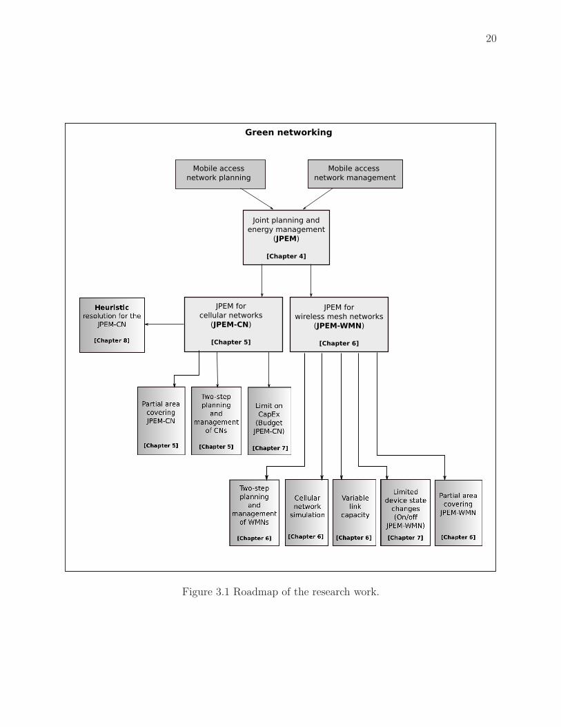
20

Mobile access

network planning

Mobile access

network management

Joint planning and

energy management

(JPEM)

[Chapter 4]

JPEM for

cellular networks

(JPEM-CN)

[Chapter 5]

JPEM for

wireless mesh networks

(JPEM-WMN)

[Chapter 6]

Green networking

Figure 3.1 Roadmap of the research work.

21

CHAPTER 4

ARTICLE 1: PLANNING FOR ENERGY-AWARE WIRELESS NETWORKS

Silvia Boiardi, Antonio Capone and Brunilde Sanso

Published on IEEE Communications Magazine, February 2014

4.1 Abstract

The paper proposes a fundamental modeling and optimization framework for the planning of

energy-aware wireless networks. The key idea is that, in order to produce an energy-efficient

network operation, energy awareness should be introduced at the planning stages. Cellular

as well as mesh wireless examples are considered.

4.2 Introduction

The rapid spread of mobile telecommunications has pushed not only for the design of new

advanced systems, but also for the development of mathematical models and optimization

algorithms to support planning and management decisions. Formal optimization methods

improve the way the limited resources (e.g., radio spectrum, base stations, antennas, back-

hauling) are used, and enhance the service quality (e.g., throughput, delay, service accessi-

bility). An important optimization problem is the general coverage planning, which consists

in determining where to locate the radio access devices and selecting their configuration so

that every client in a given area is served. This is usually the main problem addressed by

the optimization modules included within mobile operators’ software tools for radio propa-

gation estimation and network planning. The typical goal is to minimize the total antenna

installation cost while guaranteeing service coverage and quality. A nice view that helps un-

derstand the importance of network design optimization for system performance is presented

in Eisenblatter and Geerd (2006), where some modeling approaches for wireless network

planning problem are analyzed. Hurley (2002) presents an optimization framework for access

station location and configuration selection in real size cellular networks, while Eisenblatter

et al. (2010) tackles the network deployment from the wireless local area network (WLAN)

perspective. We refer the reader to the references of the cited papers for more examples.

This paper approaches the wireless network planning from a very different and novel per-

spective that accounts for energy efficiency. In recent years, the rising demand for pervasive

information access has in fact underlined the growing ICT power consumption and global

22

warming impact. Almost 50% of the power consumed by the telecommunication industry

is due to the network operation (including WLANs, LANs, mobile and fixed line systems).

Also, wireless access networks (WANs) are pointed out as the most energy hungry component

of the mobile radio segment, being responsible for over 80% of its power absorption (Boiardi

et al., 2013). As a consequence, green networking has emerged as a new way to design and

manage communication networks to reduce power consumption.

Focusing on current mobile access networks, major technical drawbacks have been identi-

fied. First, WANs are over-provisioned since they are developed to satisfy service and quality

requirements in peak traffic conditions. Second, the efforts toward energy awareness come

often at the price of a worsening of the QoS, making the analysis of the trade-off between per-

formance and energy efficiency a primary issue. There have been some attempts to consider

the energy-aware management of wireless networks by first planning a traditional network

and then optimizing its power management performance (see Section 4.3). In this article,

we convey the new and fundamental idea that energy awareness must be incorporated at the

network planning stages. Our aim is to demonstrate that the resulting network topology and

its operation are different than if planning was carried out in a traditional fashion, leaving

the energy management optimization at a later stage. The proposed approach is based on

the fact that, when power management is considered, the level of flexibility provided by the

network topology is essential to adapt the system capacity to the varying traffic load by

turning on and off unused access stations.

The framework was applied to both Cellular Networks (CNs) and Wireless Mesh Net-

works (WMNs). In what follows, after a brief review of the green network design and man-

agement techniques proposed in the literature, we introduce the philosophy underlying the

so-called JPEM problem. Then, the considered mobile systems are described, underlining the

characteristics which make them good candidates to illustrate our JPEM approach. Also,

some details regarding the optimization model formulation and its possible variations are

presented, as well as the adopted resolution approach and some example results. Our final

remarks conclude the paper.

4.3 Energy efficiency in wireless networks

In recent years, there has been a lot of work on power efficiency in wireless networks. Three

macro areas can be identified as the main focus of the research community:

• Energy-aware network design, involving issues as the deployment of heterogeneous net-

works, the use of relays and cooperative communications;

• Energy-aware network management, including, for instance, efficient routing techniques

23

able to perform traffic aggregation on a subset of links and devices, cell switch-off,

transmission rate switch and multi-RAT (radio access technology) coordination;

• Energy-aware radio technologies and hardware, consisting of methods to, among others,

improve power amplifiers efficiency (responsible alone for more than half of the access

device power consumption), deactivate device components and decrease the energy

consumption of spatial diversity techniques.

Excellent surveys which extensively treat those and other energy efficiency topics can be

found in Feng et al. (2013) and Bianzino et al. (2012).

As this paper is centered on network planning and management and not energy-efficient

radio technologies and components, we address the interested reader to the cited papers and

their references for more information. Regarding the network design research area, different

studies on energy-aware cellular networks tackle the efficiency of a radio coverage obtained

with the deployment of macro and micro cells. In Badic et al. (2009), for example, the authors

compare the power efficiency of large vs. small cell deployments on a service area using two

performance indicators: the energy consumption ratio, defined as the energy per delivered

information bit, and the energy consumption gain, quantifying the possible savings that can

be obtained by using small cells instead of big ones. Claussen et al. (2008) evaluates the

benefits of a joint deployment of macro cells and residential femtocells showing that, for high

user data rates, a mixed deployment can save up to 60% of the annual energy consumption

of the network. A similar analysis in Richter et al. (2009) considers an area where uniformly

spread users are served by a macro cell system and estimate the impact of introducing a

certain number of micro access stations in each cell. Their results show that, in case of peak

traffic scenarios, the power savings are moderate and depend on the offset power of the access

devices. A non uniform user distribution is used in Gonzalez-Brevis et al. (2011), where the

problem studied is that of finding the number and the location of micro stations in order

to minimize the long term energy consumption. The results are compared to the case of a

single macro cell serving the total number of users, and great power savings are shown for

the tested scenarios.

In the research area of energy-efficient network management, the field studying new de-

vice switch-off procedures constitutes one of the most beaten track. The minimum power

consumption of a base station (BS) can be significant, due to processing circuits and air

conditioning systems. Thus, an effective cell energy management must try to turn off as

many devices as possible. Another method is cell zooming, that allows cell size variations to

guarantee an effective area coverage while limiting the energy waste.

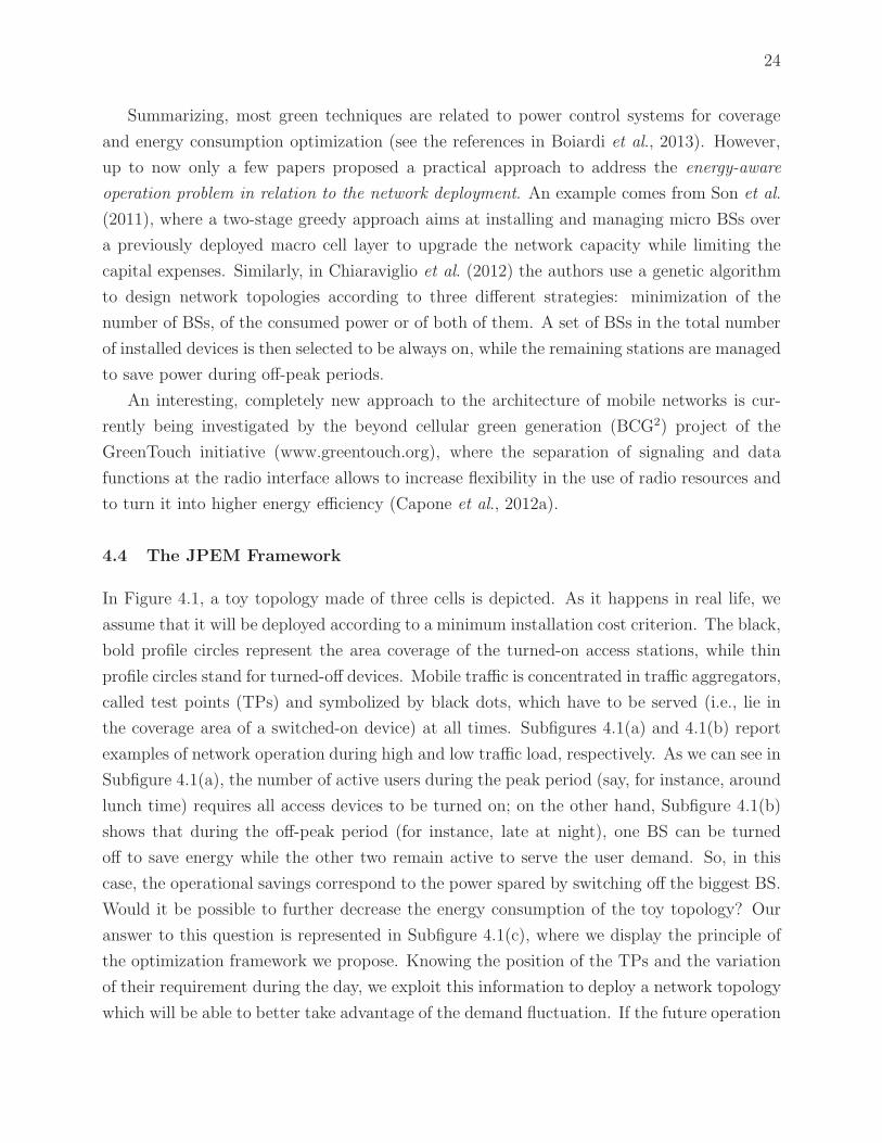
24

Summarizing, most green techniques are related to power control systems for coverage

and energy consumption optimization (see the references in Boiardi et al., 2013). However,

up to now only a few papers proposed a practical approach to address the energy-aware

operation problem in relation to the network deployment. An example comes from Son et al.

(2011), where a two-stage greedy approach aims at installing and managing micro BSs over

a previously deployed macro cell layer to upgrade the network capacity while limiting the

capital expenses. Similarly, in Chiaraviglio et al. (2012) the authors use a genetic algorithm

to design network topologies according to three different strategies: minimization of the

number of BSs, of the consumed power or of both of them. A set of BSs in the total number

of installed devices is then selected to be always on, while the remaining stations are managed

to save power during off-peak periods.

An interesting, completely new approach to the architecture of mobile networks is cur-

rently being investigated by the beyond cellular green generation (BCG2) project of the

GreenTouch initiative (www.greentouch.org), where the separation of signaling and data

functions at the radio interface allows to increase flexibility in the use of radio resources and

to turn it into higher energy efficiency (Capone et al., 2012a).

4.4 The JPEM Framework

In Figure 4.1, a toy topology made of three cells is depicted. As it happens in real life, we

assume that it will be deployed according to a minimum installation cost criterion. The black,

bold profile circles represent the area coverage of the turned-on access stations, while thin

profile circles stand for turned-off devices. Mobile traffic is concentrated in traffic aggregators,

called test points (TPs) and symbolized by black dots, which have to be served (i.e., lie in

the coverage area of a switched-on device) at all times. Subfigures 4.1(a) and 4.1(b) report

examples of network operation during high and low traffic load, respectively. As we can see in

Subfigure 4.1(a), the number of active users during the peak period (say, for instance, around

lunch time) requires all access devices to be turned on; on the other hand, Subfigure 4.1(b)

shows that during the off-peak period (for instance, late at night), one BS can be turned

off to save energy while the other two remain active to serve the user demand. So, in this

case, the operational savings correspond to the power spared by switching off the biggest BS.

Would it be possible to further decrease the energy consumption of the toy topology? Our

answer to this question is represented in Subfigure 4.1(c), where we display the principle of

the optimization framework we propose. Knowing the position of the TPs and the variation

of their requirement during the day, we exploit this information to deploy a network topology

which will be able to better take advantage of the demand fluctuation. If the future operation

25

(b) Low traffic load(a) High traffic load (c) Flexible - Low traffic load

Figure 4.1 Effect of flexibility on network operation management.

management is considered during the planning stage as in 4.1(c), an additional BS should be

installed at the cost of a slight increase in installation expenses, so as to be able to switch

off a higher number of network devices in off-peak periods (in the picture, three turned-

off BSs instead of just one). Our framework philosophy is that, by applying an energy-

aware management mechanism on a topology specifically designed to be power efficient, the

power savings can be highly increased. Therefore, differently from previous work on energy-

awareness in wireless networks, we do not assume a pre-existing infrastructure; conversely,

to improve the power management effectiveness, we argue that networks should be designed

considering the next energy efficiency requirements in the operation phase. The topologies

resulting from the application of our method demonstrate our assertions, showing that a real

energy-efficient operation strongly depends on the network coverage structure and on the

radio planning decisions taken during the design phase.

The JPEM modeling framework is based on exploiting the variety in the types of cellular

network access stations and the dynamic features of wireless mesh networks to design a

system that is not only cost-effective, but also follows the demand in an energy-efficient

way during normal operation. To the best of our knowledge, no previous modeling exist in

which energy management is incorporated into wireless network planning optimization. The

operating principle of our framework is represented in Figure 4.2, where the proposed problem

is depicted as a box having some network information as entry parameters. Such elements

constitute the basic information required as input by the JPEM framework: TP and potential

BS locations are fixed and known a priori, as well as the estimation of daily traffic patterns

and the traffic requirements in the considered time periods. Also, the types and features

(power consumption, coverage, transmitted power, installation cost) of the available network

devices are specified. Different factors are decisive in the network topology creation. The

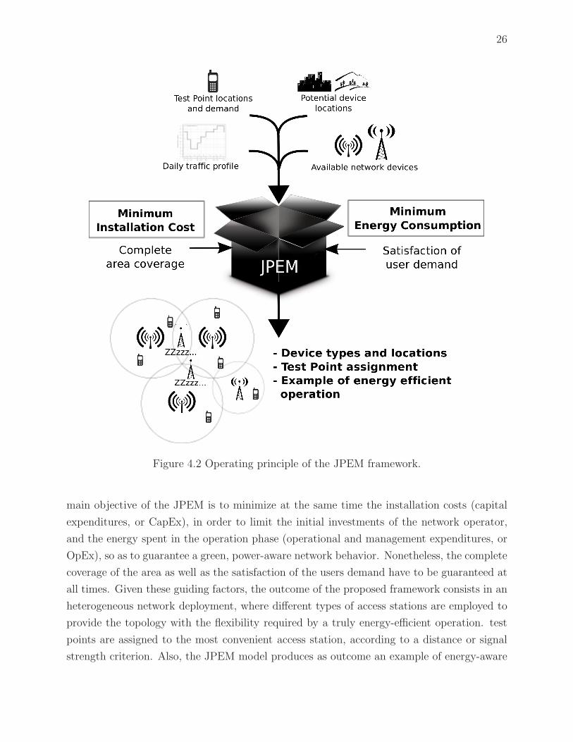
26

Figure 4.2 Operating principle of the JPEM framework.

main objective of the JPEM is to minimize at the same time the installation costs (capital

expenditures, or CapEx), in order to limit the initial investments of the network operator,

and the energy spent in the operation phase (operational and management expenditures, or

OpEx), so as to guarantee a green, power-aware network behavior. Nonetheless, the complete

coverage of the area as well as the satisfaction of the users demand have to be guaranteed at

all times. Given these guiding factors, the outcome of the proposed framework consists in an

heterogeneous network deployment, where different types of access stations are employed to

provide the topology with the flexibility required by a truly energy-efficient operation. test

points are assigned to the most convenient access station, according to a distance or signal

strength criterion. Also, the JPEM model produces as outcome an example of energy-aware

27

operation of the chosen topology where, in line with the daily traffic pattern, unused BSs are

switched off to reduce the power consumption.

4.5 Examples

Two examples illustrate how the JPEM framework can be used to design energy-aware wire-

less networks and to analyze the trade-off between installation cost and power efficiency.

They are based on cellular networks, which are the most important and popular wireless

access technologies, and wireless mesh networks, that add the issue of multi-hop coverage.

4.5.1 Cellular Networks

The reference system for the Cellular Network model can be described as follows. Given an

area to be served, a set of Traffic test points (TTPs) representing traffic centroids is picked

out. Besides, a new set of Coverage test points (CTPs) is introduced. Differently from the

former, they do not produce any traffic; rather, they are disposed on a regular grid overlaying

the area to ensure the total coverage in the dimensioning phase even in the off-traffic regions.

Together with the TPs, a set of available candidate sites (CSs) where the BSs are allowed

to be positioned is identified. Since the signal propagation between any pair of TP and CS

can be measured or evaluated, the subset of TPs reached by a sufficiently strong signal is

assumed to be known for a BS installed in any CS. In particular, we calculated the median

path loss by mean of the COST-231 Hata model. Shadowing and fast fading effects are

neglected, which is a common assumption in network design modeling. The framework is

however general enough to accept other types of propagation models.

To account for traffic load fluctuation typical of real networks, a daily pattern reflecting

mobile user habits and representing the active user percentage at each time is considered.

The day is then split in periods where the TTP’s traffic demand, given by a random value

uniformly chosen between a minimum and maximum values, is considered unchanged. Al-

ternatively, TTPs can be in idle state if no traffic is requested. Note that long term demand

variations are not taken into account. However, the method is applicable independently of

the characteristics of the traffic changes.

Finally, according to the key idea that flexibility is a fundamental characteristic for a

power-efficient network, we decided to exploit the diversity offered by the market in terms

of cell dimension. Therefore, several BS configurations are made available, having different

installation cost, capacity, consumed power, transmitted power and coverage.

28

4.5.2 Wireless Mesh Networks

wireless mesh networks (WMNs) are a type of dynamically self-organized and self-configured

communication infrastructures that offer wireless connectivity through the use of cheap and

low transmission power devices. Each node in WMNs works as a host as well as a router,

forwarding packets on behalf of other nodes that may not be in the transmission range of their

destinations. Thus, the nodes automatically establish mesh connectivity among themselves,

creating in effect an ad-hoc network.

In the JPEM framework, the mesh reference system is made up of mesh routers (MRs)

and mesh access points (MAPs), which communicate through dedicated wireless channels

with other access devices residing in their coverage radius. Routers and gateways (generally

referred to as BSs) can be installed only in pre-determined CSs. Both kinds of BSs provide

network access to mesh users; in addition, MAPs, representing only a restricted set of routers,

behave as gateways toward the wired backbone, enabling the integration of WMNs with other

networks (typically the Internet). Concerning mesh clients (MCs), they can be assigned to

only one BS, being the closest active one, and are connected to the Internet through multi-hop

communications.

The day is also divided in time periods during which mesh clients require a fixed amount

of traffic. Again, the traffic profile is defined as the percentage of active users typical of every

time interval, but in this case two different congestion levels are considered. In addition to

the standard profile, a busy profile has been tested, characterized by a higher value of the

minimum user demand.

4.5.3 JPEM Implementation

Let us analyze first the case of cellular networks. From the perspective of power consumption

per unit of covered area, a network topology based on small and low-power cells is generally

considered more convenient than one deploying only high-power cells. However, since per-

site fixed installation expenses tend to prevail, a small cell topology involves high deployment

costs. Now, considering that active users must be provided with network service at all time,

a cellular system only based on small cells may not be the most energy efficient option; in

this case, all cells would be necessary to provide full area coverage and none of them could be

switched off during low-traffic periods. Conversely, the availability of different network con-

figurations, employing a set of BSs with different capacity and energy consumption, is what

we point out as the key issue to enable effective power management strategies. Such a topol-

ogy can be obtained only if network planning and operation management are incorporated

in the same optimization framework.

29

min

Figure 4.3 JPEM implementation for Cellular and Wireless Mesh Networks.

The JPEM for Cellular Networks (JPEM-CN) is a binary linear programming model to

jointly plan and manage cellular networks. The schematic of JPEM-CN is reported in Fig-

ure 4.3(a), while we refer the reader to Boiardi et al. (2013) for the mathematical formulation

and further details. Through three sets of binary decision variables, identifying i) the BS

configurations installed in the selected CSs, ii) the state (on/off) of every installed BS and

iii) the assignment of TTPs to one of the turned-on BSs, the model attempts to minimize an

objective function without violating a set of constraints on the variable values. The objective

function can be broken down in two main terms. The first one, namely CapEx term, accounts

for the installation cost of the chosen devices; the OpEx term, on the other hand, considers

the energy consumption in the operational setting, summing up the power required by each

BS during the time periods in which it is turned on. In the cellular context, a third term

distance TP/CS, to promote the assignment of TPs to the most convenient access device (in

terms of distance or signal strength) was introduced in the objective function. Interestingly,

that term was active only with GSM technology, whereas it did not have any impact for

LTE networks. In order to fairly compare the OpEx term, consisting in a measure of power

consumption, with the CapEx one, consisting in a high, one-time cost, the energy related

expenses are calculated over the network lifetime (assumed to be 14 years). The trade-off

between CapEx and OpEx is adjusted by a weight parameter β, which varies from 0 to any

big integer value (typically between 1 and 10). When CapEx are the only costs to be min-

imized, the value of β is set to 0 to exclude the OpEx term from the objective function:

this way, the resulting network installs the minimum cost topology. On the other hand, by

choosing higher values for β and introducing the OpEx in the objective function, the model is

pushed by the energy management mechanism to reduce at the same time capital and opera-

tional expenses. The JPEM-CN framework seeks to minimize the objective function provided

30

that some fundamental constraints are respected. Commonly used in network dimensioning

problems, coverage constraints provide a basic and constant coverage of the service area,

guaranteeing that all the TPs, being Coverage or Traffic ones, lay in the coverage area of at

least one switched-on BS (coverage constraints can be relaxed when architecture based on

signaling and data separation are considered, as suggested in Capone et al., 2012a). Assign-

ment constraints ensure that every TTP is served by one BS in each time period. Traffic

TPs in idle state (i.e., that are not requesting traffic in a certain time interval) are as well

assigned to a BS, but they do not contribute to fill its capacity. Also note that for Coverage

TPs, which never provide traffic, the explicit assignment to an access station is not required.

Each access station can route the traffic of a limited number of Traffic TPs, depending on its

capacity and therefore on the chosen configuration. So, capacity constraints guarantee that

active BSs are able to satisfy the traffic demand of the assigned TTPs at any time. Other

sets of constraints are introduced in the model formulation, relating the values of different

decision variables and fixing their binary domain.

The joint framework for wireless mesh networks (JPEM-WMN) (see Figure 4.3(b) for a

schematic and Boiardi et al., 2012b, for the complete formulation) utilizes the same set of

decision variables as JPEM-CN: device installation, activation and user assignment. Fur-

thermore, new variables are introduced to keep track of the wireless link existence and usage

between MRs, MAPs and the Internet. Once again, the objective function represents the

trade-off between the CapEx, corresponding to the installation costs of MRs and MAPs, and

the OpEx, calculated as the power expenses of the active devices in any time interval. In this

case, the parameter δ weights the relative importance of the two terms by assuming values

in the [0,1] interval. Starting from δ = 1, when just capital expenses are minimized, we grad-

ually reached the opposite case of δ = 0 (minimization of power costs only) after evaluating

intermediate values. Due to the difference between cellular and mesh system structures, in

addition to the well-known sets of coverage, assignment and capacity constraints, different

sets of link and traffic flow constraints are added to the WMN formulation.

4.6 Main results

In order to illustrate the advantages in energy savings achievable by the new planning frame-

work, we show two examples of CN and WMN application. The results are obtained by

solving the described linear binary models with CPLEX branch and bound solver, which

produced optimality gaps below 5%. Resolution time varied from a few seconds to about half

an hour.

Tables 4.1 and 4.2 report the total CapEx required by the network deployment and the

31

Table 4.1 Results from CN Scenario with different values of β.

β = 0 β = 0 β = 1 β = 10(two-step) (joint) (joint)

CapEx (k¤) 56 56 62 (+11%) 66 (+18%)OpEx (k¤, 14 years, 0.2¤/KWh) 42 39 19 17

OpEx vs. no management - -7% -55% -60%OpEx vs. two-step - - -51% -56%

Installed BSs 18 18 17 21BS Type Macro - 1 Macro - 1 Macro - 0 Macro - 0

Micro - 1 Micro - 1 Micro - 5 Micro - 5Pico - 16 Pico - 16 Pico - 12 Pico - 16

Table 4.2 Results from WMN Scenario with different values of δ.

δ = 1 δ = 1 δ = 0.5 δ = 0.1(two-step) (joint) (joint)

CapEx (k¤) 9.6 9.6 10 (+4%) 12.4 (+29%)OpEx (k¤, 14 years, 0.2¤/KWh) 17.2 15.6 13.5 13.1

OpEx vs. no management - -9% -21% -23%OpEx vs. two-step - - -14% -16%

Installed MRs 44 44 46 50Installed MAPs 2 2 2 6

expected OpEx, calculated over a fourteen-year network lifetime by considering an energy-

aware network operation management. Both values are expressed in thousands of Euro, while

we assume an energy cost for business users of 0.2 ¤/kWh. The percentages in parenthesis

show the CapEx increase with respect to the minimum installation cost topology. Two other

sets of percentages are displayed. The first group (third row) indicates the OpEx reduction

compared to first column results, while the second group (fourth row) shows the operational

cost decrease with respect to the second column ones. The next tables entries represent the

number and type of installed BSs, being macro, micro or pico cells in the cellular network

case or MRs and MAPs in the wireless mesh network one.

Let us now discuss Table 4.1, where the most important results for a long term evolution

(LTE) cellular system scenario are displayed. The service area is a 4 km2 square, over which

40 CSs, 121 Coverage TPs and 30 Traffic TPs are located. Each traffic demand is a random

value uniformly chosen between 20 and 40Mb/s. The first column, β = 0, describes the case

of a cellular network deployment based on the minimum CapEx network planning where no

energy management is performed. A two-step procedure is represented in the second column;

here, optimization is first performed without considering the running costs and then, network

operation is independently optimized by applying an energy-aware management mechanism

32

to the obtained topology. β = 1 and β = 10 correspond to the case of joint design and

management optimization, where the value of the weight parameter symbolizes the relative

importance of the OpEx term with respect to the CapEx one in the model objective function.

The most important information included in the table regards the variations in the deployed

network when the two-step or joint framework are adopted. By increasing the value of β,

and so introducing energy-awareness in network planning, different types and numbers of BSs

are installed. In particular, a higher number of medium or small BSs tend to be preferred

to macro cells, which have high installation cost and power requirements. Also, from an

energy point of view, macro BSs can hardly be turned off to save power during off-peak

periods due to their large coverage radius. It appears straightforward that, when we allow

the joint framework to account for the network energy consumption at the planning stage,

great energy savings are enabled at the cost of a modest increase in CapEx. For instance,

with easy calculations we find that when the trade-off parameter is set to 1, the extra capital

investment, corresponding to 6000 ¤, can be recovered in slightly more than four years from

the savings in network operation, amounting to 1450 ¤ per year.

The same observations made for cellular networks apply to the wireless mesh network

instance reported in Table 4.2. Here, when the trade-off parameter δ decreases, the proposed

optimization model is pushed to optimize the network topology and operation in a joint way.

On the other hand, if δ equals 1, the less expensive topology from the CapEx perspective is

installed and an energy-aware management mechanism can be carried out in a second stage.

TheWMN scenario displayed in the table includes 240 MCs, requesting a traffic between 1 and

10 Mb/s, and 64 CSs placed over a square area with side 2.5 km. As for Cellular Networks,

we notice that a growing number of routers (MRs) is deployed when the operational savings

assume more importance than the minimization of the CapEx. Also, when δ = 0.1, four

additional MAPs are selected: the power savings are further increased by adding Internet

access points, this way limiting the number of hops (i.e., active MRs) necessary for the MC’s

traffic to reach its destination. Yet again, the OpEx saving percentages confirm the soundness

of our framework. However, in this case, we note less striking results due to the fact that

WMNs present a limited choice in the device selection, allowing just one configuration of

router and one of access point to be deployed. This aspect validates further our initial claim

that the network flexibility represents the most important element to enable an effective

energy-efficient network behavior.

Results from different test scenarios and interesting framework variations (the relaxation

of the total area coverage constraints, among others) can be found in our previous work

Boiardi et al. (2013) and Boiardi et al. (2012b).

33

4.7 Conclusion

Recent studies on green networking show that a network operation management that follows

the traffic variations is one of the most useful instruments to reduce power consumption.

In this paper we have shown that, by minimizing at the same time installation costs and

operation power expenses, networks are designed for a more efficient energy-aware operation.

With the help of some results from Cellular and wireless mesh networks, we showed that an

optimal topology from the installation cost point of view does not produce a network that

is optimal for an energy-aware perspective. Conversely, the most power-efficient networks

include different types of devices, providing the management mechanism with the required

flexibility to adapt the network capacity to the user demand in different time periods.

Even though our proposal has specifically focused on energy-awareness on-off operation,

it would still be valid for other type of operational issues, such as on-line antenna tilting, for

instance (Tipper et al. (2010)). In the end, our proposed framework can be summarized in

adding and optimizing flexibility at the planning stages for a more efficient and cost-effective

operation.

34

CHAPTER 5

ARTICLE 2: RADIO PLANNING OF ENERGY-AWARE CELLULAR

NETWORKS


Published on Computer Networks, September 2013

5.1 Abstract

This paper introduces a joint planning and management optimization approach for cellular

networks to limit energy consumption while guaranteeing QoS and minimizing operators’

CapEx and OpEx. The modeling framework shows that an effective energy-efficient operation

depends on the planning decisions. Conversely, it also shows that planning with energy

management operation in view yields more versatile topologies than more traditional models

based only on CapEx. Results for LTE networks are provided and show that savings up to

65% in energy expenses are possible with slight increases in capital investments.

5.2 Introduction

It has been reported (The Climate Group, 2008) that the ICT sector is responsible for the

world energy expenditures for a percentage that ranges from 2% to 10%. Of particular concern

is the consumption of the cellular wireless system, both for its increasing pervasiveness that

pushes for more wireless infrastructure and for the well known fact that base stations (BSs)

are particularly energy-hungry, representing over 80% of the power used in the radio segment.

While responsibility for climate change is the main push for green networking research,

network operators are equally interested in energy consumption reduction for economic rea-

sons. Two types of cost are incurred: CapEx, related to the purchase and installation of

radio equipment, and OpEx, consisting on energy, site rentals, marketing and maintenance

costs (Johansson et al., 2004). The challenge in terms of energy-aware modeling is to convey

both types of cost and power issues into a single modeling framework, which is precisely the

objective of this paper. The only example of energy-aware joint design and management

method is presented in our recent work Boiardi et al. (2012b), where we introduced a sim-

ilar approach for mesh networks and provided multiple examples and model variations for

supporting our thesis. However, to the best of our knowledge, the problem has never been

tackled from the cellular network point of view.

35

The article is divided as follows. In Section 5.3 the modeling framework philosophy is

introduced, while Section 5.4 reports general as well as wireless green networking literature.

The propagation model, the traffic variations in time and the different types of BSs con-

sidered in the model are exposed and discussed in Section 5.5. The model itself, based on

mathematical programming, is presented in Section 5.6. The resolution approach, including

the instance generation process and some additional tests, is discussed in Section 5.7 together

with numerical results, whereas Section 5.8 concludes the paper.

5.3 Proposed modeling framework

From an energy savings standpoint, a radio coverage obtained using small cells served by BSs

with low power is considered more convenient in terms of energy per covered area than one

with macro cells of high power BSs (this may not be true for all power profiles of devices, but

the trend in device technology is going in that direction, Greentouch, 2010). In fact, when

the cell radius is reduced, the energy consumption usually decreases faster than the increase

of the number of BSs required to cover the area. The opposite is achieved with deployment

costs, due to the fact that per-site fixed installation costs tend to prevail. Now, considering

that the full coverage of the service area must be ensured at all times, a cellular system based

only on small cells may not be the most energy efficient option since all cells are necessary to

provide full coverage and none of them can be turned off when traffic is low. On the contrary,

the availability of a potentially large number of network configurations, consisting in a set of

active BSs having different capacity and energy consumption levels, is the key issue to enable

efficient energy management strategies.

Therefore, claiming the key role of network flexibility and stating that energy management

must be considered when planning the radio coverage of the cellular network, here we propose

an approach that jointly optimizes the network design, based on CapEx and OpEx costs, as

well as the power management according to different traffic levels.

The traditional models for wireless access network planning - including 2G (Mathar and

Niessen, 2000), 3G (Amaldi et al., 2003) and Wireless LANs (Bosio et al., 2007) examples -

have to do with finding locations and configuration settings for network devices in order to

serve the traffic demand while matching service requirements. The optimal radio planning

problem, which consists in determining the best BSs locations out of a set of candidate sites

(CSs) while insuring an appropriate signal level, results in the classical minimum cost set

covering problem. Taking this basic radio planning model as starting point, we introduce the

following innovative features to produce the joint design and management framework: i) The

objective function not only includes BSs installation costs (CapEx) but also operational ones

36

(OpEx), assuming that their variable part is largely due to the expenses related to the energy

consumption; ii) Variables and constraints are redefined to include the energy management

mechanism in the model and a set of traffic demands related to different time periods of the

day is introduced; iii) A trade-off parameter defines the relative importance of CapEx and

OpEx in the optimization process and can be used to compare our results with traditional

CapEx-only network planning or two-step planning and management approaches (see Section

5.7.3).

5.4 Related Work

Since the seminal work of Gupta and Singh (2003), there has been an expansion in green

networking research. Regarding wireless networks, examples of exhaustive reviews of green

mobile opportunities can be found in Koutitas and Demestichas (2010); Wang et al. (2012b).

Three case studies for reducing BS power consumption are reported in Han et al. (2011),

while other detailed investigations on energy awareness in cellular networks are described in

Hasan et al. (2011); Correia et al. (2010).

Although a large body of literature is focused on energy-efficient devices or protocols, more

recent efforts are on planning or operation, but always tackling the design andmanagement as

separate problems. Considering network operation optimization, a great amount of work has

appeared in the last few years. In Chiaraviglio et al. (2008b), given the network topology and

a fixed traffic demand, the possibility of switching off some nodes to minimize the total power

consumption while respecting QoS is evaluated. However, no traffic variations in space or time

are considered. Deterministic traffic variations over time are taken into account in Lorincz

et al. (2010) as well as in Marsan et al. (2009), where the energy saved by reducing the

number of active access devices when they are not fully utilized is characterized for different

cell topologies. In Chiaraviglio et al. (2008a) the authors show that it is possible to switch

off some UMTS Nodes in urban areas during low-traffic periods, still guaranteeing quality

of service constraints in terms of blocking probability and electromagnetic exposure limits,

while authors in Zhou et al. (2009) consider a random traffic distribution and dynamically

minimize the number of active BSs to meet the traffic variations in both space and time

dimensions. Moreover, Weng et al. (2011) examines the cell zooming problem (i.e., the

extension of a cell coverage area to guarantee service when other BSs are turned off) and

assesses the possibility of modifying the cell deployment to allow higher power savings by

turning off a greater number of BSs.

For what concerns network planning, Badic et al. (2009) measures the power efficiency of a

large vs. small cell deployment on a service area by the help of two performance metrics: the

37

energy consumption ratio, defined as the energy per delivered information bit, and the energy

consumption gain, which quantifies the possible savings obtaining using small cells instead

of big ones. In Qi et al. (2010) the authors divide the service area into dense and sparse

zones and propose an adaptive deploying strategy where the size of the cells can be adjusted

according to the varying user requests. Paper Claussen et al. (2008) evaluates the effectiveness

of the joint deployment of macro cells and residential femtocells, while Richter et al. (2009)

investigates the cells layout impact on power consumption by varying the numbers of micro

BSs per cell in addition to conventional macro sites. The results they provide show that the

power savings are moderate in case of peak traffic scenarios and depend on the offset power of

the BSs. Unlike such work, we do not limit our analysis to regular layouts and we propose an

optimization approach that can be used with arbitrary topologies and propagation scenarios.

Up to now, only a few articles approached the problem of optimizing the network deploy-

ment and the energy-aware operation at the same time. In particular, the trade-off between

deployment efficiency and energy efficiency is pointed out as one of the fundamental frame-

works in green radio research in Chen et al. (2011), while Chen et al. (2010) treats it in more

details, defining an analytical relation between the two terms. Another approach in the use of

micro cells overlapping a pre-existing network is discussed in Son et al. (2011), where a two-

stage greedy approach is used to upgrade the network capacity while limiting the required

expenses. In the first stage, additional micro BSs are installed over a previously deployed

macro cells layer to meet peak traffic demand; then, the network operation is managed with

the aim of reducing power waste during off-peak periods. Differently from that article, we do

not assume a pre-existing infrastructure but rather find what that infrastructure should be

by jointly optimizing the planning (BS location and type) and the energy efficient operation.

Moreover, not only the peak demand but all the varying demand scenarios are included in

the optimization framework. A similar two-stage planning and management technique is also

adopted in Chiaraviglio et al. (2012). Here, the authors exploit a genetic algorithm to design

network topologies according to three different strategies: minimization of the BSs number,

of the consumed power or of both of them. A set of BSs in the total number of installed

devices is then selected to be always on, even during off-peak traffic periods; the next step

consists in managing the remaining access stations in order to save power when traffic is low.

BSs are turned off according to two criteria: least loaded (lower number of served users) and

most overlapped (highest portion of coverage area shared with neighbor BSs). In our work,

contrarily, we adopt a one-step approach to point out the benefits and the topology changes

that can be obtained when the network design and management are optimized in a joint

fashion.

38

5.5 Preliminaries

5.5.1 Base Station Categories

In order to verify our claims and evaluate the proposed approach, we considered LTE technol-

ogy test scenarios. Since we stated that network flexibility is a key factor to obtain an effective

energy-efficient network management, three different BS types (called here configurations)

are taken into account, each one allowing to be switched off in case of low traffic profile.

Realistic power consumption and capacity values for BSs have been extracted from Imran

(2011) and collected in Table 5.1, where the heading “Consumed Power” represents the mean

equipment power consumption (including power amplifier, signal generator, air conditioning

and microwave link). Note that we provide specific BS categories to create interesting nu-

merical examples, but the proposed design approach is general and can be used with any mix

of BS types and technologies.

5.5.2 Traffic Variation Behavior

Intuitively it can be said that traffic intensity varies as a natural effect of users daily habits.

For example, it has been measured that mobile traffic presents its peak between noon and 4

pm and that there is a significant decrease in the late evening. Moreover, in a typical business

area, the traffic pattern is almost the same from Monday to Friday but it decreases during

the weekend (see Heegaard, 2007). To account for the main fluctuations, but neglecting the

differences that occur between working and weekend days, we consider an approximated daily

pattern based on the downlink traffic measurements presented in Imran (2011). According to

this profile the whole day is split in time periods, each one gathering smaller intervals (hours)

in which the users behavior can be assumed unchanged. We define T as the ordered set of

time periods, with δt representing the length of period t ∈ T . The end of each time period is

equal to the beginning of the new one, so that there is no time gap between adjacent periods

and the summed duration of all periods is equal to the number of hours in a day. In this

paper, we assume a total of eight time periods for our LTE examples. Observing Figure 5.1,

the progress of the approximated traffic profile defines active user percentages in every time

interval.

In more detail, our traffic distribution is modeled as follows. Let us define a test point (TP)

as an aggregated traffic centroid. From now on, we will refer to typical TPs with the name

of Traffic test points. For each Traffic TP we calculated a random value uniformly chosen

between 20 and 40 Mb/s, together with a random number in the [0, 1] interval. The first

value is fixed, denoting the traffic amount that each Traffic TP provides to the network only if

the second number is less or equal the normalized traffic value. Furthermore, in our modeling

39

Table 5.1 Transmission and consumption features of each BS configuration.

Installation Transmitted Consumed Traffic CoverageConfiguration Cost Power Power Capacity Distance

(¤) (dBm/W ) (dB/W ) (Mb/s) (m)

C1 30000 43 / 19.9 31.3 / 1350 210 1230C2 10000 38 / 6.3 21.6 / 144.6 70 850C3 1000 21 / 0.1 11.7 / 14.7 70 241

framework we introduce a new kind of Coverage test points, disposed on a regular square

grid overlaying the whole area. Coverage TPs do not produce any traffic but, since they have

to lie in at least one active cell, they are essential to ensure the total area coverage in the

dimensioning phase even in the off-traffic regions.

5.5.3 The Propagation Model

Although, in real scenarios, the transmitted signal quality is affected by path loss, shadowing

and fast fading, a common assumption in network modeling consists in omitting shadow-

ing, while we neglect fast fading because of the characteristics of our problem (small-scale

variations are fairly rapid in space).

Being f (2600 MHz) the operating frequency, hb (12m, 10m or 8m according to the

BS configuration) and hr (1.5m) the correction factors for BS and user antenna height, the

median path loss at a generic distance d is calculated by using the COST-231 Hata model

(Hata, 1980):

PL(d)[dB] = 46.3 + 33.9Log(f)− 13.82Log(hb)− a(hr)+

+ (44.9− 6.55Log(hb))Log(d) + cm.(5.1)

The parameter cm is equal to zero for suburban areas, while the function a(hr) is defined as:

a(hr) = (1.1Log(f)− 0.7)hr − (1.56Log(f)− 0.8). (5.2)

Finally, cable losses are 2 dB while antenna gains are assumed to be 15 dB for configurations

C1, C2 and 12 dB for C3.

5.6 The Joint Design and Management Framework

Let us define the model parameters:

40

Time

Nor

mal

ized

Tra

ffic

Pat

tern

0h 2h 4h 8h 10h 13h 18h 20h 24h

00.

10.

20.

30.

40.

50.

60.

70.

80.

91

t1 t2 t3 t4 t5 t6 t7 t8

Approximated Traffic Pattern

Figure 5.1 Approximated traffic profiles for LTE systems.

Ic : Set of Coverage TPs, which do not generate any traffic but help provide a basic, fixed

network coverage even in case of very low traffic profile.

It : Set of Traffic TPs, which allow the network to “follow” traffic changes in the different

time periods by generating variable traffic.

S : Set of available CSs for the BSs.

Kj : Set of possible configurations for a BS located in site j ∈ S.

T : Set of time intervals.

δt : Duration of time period t ∈ T .

pit : Traffic provided by the Traffic TP i ∈ It in period t ∈ T .

cjk : Capacity of the BS located in site j ∈ S with configuration k ∈ Kj.

γjk : Installation cost for a BS located in site j ∈ S with configuration k ∈ Kj . This is

41

composed of the cost due to the characteristics of the chosen site (for example, open

spaces or buildings) and the cost specific for the selected configuration.

ǫjk : Power consumption for a BS located in site j ∈ S with configuration k ∈ Kj.

rij : Distance between the Traffic TP i ∈ It and the BS located in site j ∈ S.

ϕ : Cost of the energy consumption over the entire network life. This parameter is defined

as E · 365 · n · 0.001, where E represents the energy cost (¤) per kWh, n stays for the

years over which the OpEx costs are computed (365 days in a year), and the factor

0.001 is used to convert from Wh to kWh. In this paper, we will consider E = 0.35

¤/kWh and n = 8, which lead to ϕ = 1.

β, ϑ : Weight parameters that will be used for trading-off the objective function.

To conclude the model parameters, we need to introduce a binary one that summarizes

the coverage information for each combination of TP and CS:

aijk =

1 if TP i ∈ Ic ∪ It is in the coverage area of a BS

installed in j ∈ S with configuration k ∈ Kj ,

0 otherwise.

(5.3)

Let us now define the z, y and x decision variables that represent, respectively, the choice

of BS location and configuration type, the BS status (active or idle) and the TP assignments:

zjk =

1 if a BS is installed in site j ∈ S with configuration

k ∈ Kj ,

0 otherwise.

(5.4)

yjkt =

1 if a BS installed in site j ∈ S with configuration

k ∈ Kj is active in period t ∈ T ,

0 otherwise.

(5.5)

xijt =

1 if TP i ∈ It is assigned to a BS in site j ∈ S in

period t ∈ T ,

0 otherwise.

(5.6)

42

Then, the JPEM-CN can be defined as follows:

min∑

j∈S

∑

k∈Kj

zjkγjk+β ϕ∑

j∈S

∑

k∈Kj

∑

t∈T

ǫjkδtyjkt+ϑ∑

i∈It

∑

j∈S

∑

t∈T

xijtδtrij (5.7)

subject to:∑

j∈S

∑

k∈Kj

aijkyjkt ≥ 1 ∀i ∈ Ic ∪ It, t ∈ T (5.8)

xijt ≤∑

k∈Kj

aijkyjkt ∀i ∈ It, j ∈ S, t ∈ T (5.9)

∑

i∈It

xijtpit ≤∑

k∈Kj

cjkyjkt ∀j ∈ S, t ∈ T (5.10)

∑

j∈S

xijt = 1 ∀i ∈ It, t ∈ T (5.11)

yjkt ≤ zjk ∀j ∈ S, k ∈ Kj , t ∈ T (5.12)∑

k∈Kj

zjk ≤ 1 ∀j ∈ S (5.13)

zjk ∈ {0, 1} ∀j ∈ S, k ∈ Kj (5.14)

xijt ∈ {0, 1} ∀i ∈ It, j ∈ S, t ∈ T (5.15)

yjkt ∈ {0, 1} ∀j ∈ S, k ∈ Kj , t ∈ T (5.16)

The objective function (5.7) is composed of three parts: the CapEx term, which accounts

for the equipment installation costs, the OpEx one, that considers the energy expenses over

the entire network lifetime, and a final term to guarantee a better connection quality between

users and antennas. In the case of the results presented in this paper, however, we verified

that the third component, introduced to push the assignment of each TP to the nearest

available BS, does not have any influence on the choice of the serving BS. For this reason, we

set the trade-off parameter ϑ to 0. On the other hand, by playing with the trade-off parameter

β, the relative weight of the CapEx and OpEx components can be modified. Setting β to 0,

OpEx costs are excluded from the objective function and only the installation investments

are minimized: the resulting network will deploy a minimum cost topology. When β is equal

to 1, the energy management mechanism is enabled and forces the model to reduce not only

capital but also operational costs by introducing the OpEx term in the objective function.

Finally, higher values of β show the network topology changes and the greater energy savings

that can be obtained when growing importance is given to the OpEx component. Concerning

constraints, we introduce two sets of coverage constraints. (5.8) provide a minimal, constant

coverage by ensuring that all the TPs are within the service area of at least one active BS,

while (5.9) assign Traffic TPs only to a BS they are covered by. Capacity constraints (5.10)

guarantee that each active BS can satisfy the traffic demand of the assigned Traffic TPs

43

and assignment constraints (5.11) impose that every Traffic TP is assigned to only one BS.

(5.12) are linking constraints between variables y and z, while configuration constraints (5.13)

impose that at most one BS configuration is installed in a CS. Finally, (5.14), (5.15) and

(5.16) impose the binary values for the decision variables.

JPEM-CN, which is a linear binary problem, is NP-hard.

5.7 Resolution Approach and Numerical Examples

5.7.1 Instance Generation

The proposed mathematical model was implemented on AMPL and solved with CPLEX

branch and bound solver (CPLEX, I.B.M., 2010), which produced optimality gaps below 5%

for the experimented instances. The resolution time ranged from a few seconds to approx-

imately half an hour, depending on the value of β and on the scenario dimension. To test

the effectiveness of the proposed model, we designed and implemented in C++ an Instance

Generator which creates realistic cellular network scenarios where the number of CSs and

TPs is similar to the one that can be found in real networks. The features of our test sce-

narios are described in Table 5.2: the first entry represents the area size (expressed in square

kilometers), the second one is the number of CSs randomly located in the considered region

and next are the number of Coverage TPs (CTPs), placed on a regular grid which covers the

service area. The last entry displays the number of Traffic TPs (TTPs), evenly randomly po-

sitioned in the whole area (Scenario 1 and 2) or placed with a higher probability in a smaller

region that can represent, for example, a built-up area in the countryside or the center of a

big city (Scenario 3-3a-3b-3c). For every scenario, different values of the weight parameter β

were tested: by doing so, we strove to highlight the benefits achieved by jointly minimizing

costs and power expenditures in the design and management phases, instead of limiting the

optimization at the network planning stage.

5.7.2 Additional Tests

In order to evaluate the value of the proposed approach, we compared our results with

those obtained by separately optimizing, first, the network design, and then, the network

management. The common two-step approach has been reproduced by adapting our model

in the following steps:

1. Run the JPEM-CN with β = 0 to choose the minimum cost topology without consid-

ering the energy management;

44

Table 5.2 Parameters used to generate the test scenarios.

Area (km2) CSs CTPs TTPs Allowed Configurations

Scenario 1 2×2 40 121 30 AllScenario 2 5×5 60 676 60 AllScenario 3 4×4 120 441 40 All

Scenario 3a 4×4 120 441 40 C1, C2Scenario 3b 4×4 120 441 40 C1, C3Scenario 3c 4×4 120 441 40 C2, C3

2. Fix variables zjk according to the results of the previous step: this way, locations and

characteristics of installed BSs will be defined;

3. Run the joint model where zjk are no longer variables but parameters set according to

step 2 (network topology is already defined) and the CapEx term is excluded by the

objective function.

Moreover, since data traffic in cellular networks is typically bursty (that is to say, users

are likely to provide traffic only in certain time intervals, while they are silent for the rest of

the time), we observed that greater energy savings could be reached if the network service

was limited only to active Traffic TPs. So, as JPEM-CN, this problem variation aims at

providing a full-coverage network deployment, but now the objective is that of guaranteeing

service only to the users that are requiring traffic in any time period, allowing to turn off

those BSs which have only inactive users in their coverage region. To model the partial

coverage approach, we need to introduce a new set of binary parameters mit that are equal

to 1 if Traffic TP i is active in time period t. Then, constraints (5.8) in the original model

are replaced by:∑

j∈S

∑

k∈Kj

aijkzjk ≥ 1 ∀i ∈ Ic ∪ It, (5.17)

meaning that every Coverage or Traffic TP has to be covered by an installed BS, regardless

of its on or off state, while constraints (5.11) become:

∑

j∈S

xijt = mit ∀i ∈ It, t ∈ T, (5.18)

since network service is provided only to active clients. The partial coverage problem can be

written as:

min (5.7)

subject to (5.9), (5.10), (5.12)− (5.18).

45

Note that the partial coverage case cannot be implemented in current mobile network tech-

nologies where continuous and full coverage must be ensured. However, new access archi-

tectures have been recently proposed and are currently being considered by standardization

bodies where the control and data plane are separated at the the radio interface (Capone

et al., 2012a). Such a separation allows data BSs to be turned off when no active user is un-

der their coverage area, since a continuous access availability is guaranteed by the always-on

signaling BSs.

5.7.3 Numerical Results

In order to appreciate the results of the joint approach and the differences with the two

proposed variations, in what follows we concentrate mainly on pictures representing some

important results from Scenario 2. Traffic TPs are symbolized by black dots, while Coverage

TPs are arranged on a regular grid every 200m. Only selected CSs are depicted: switched-on

BSs are represented as black triangles, while switched-off BSs as white ones.

Let us focus on Figure 5.2, which displays the network obtained for Scenario 2 when the

CapEx and OpEx are optimized in two separate steps. Since in the first step only capital

costs are minimized, the network planning recalls the capacitated facility location problem

and the installed BSs represent the minimum cost network topology. We note that as much as

5 type C1 BSs are deployed and, together with 11 additional type C2 BSs, they can cover the

whole area. However, due to the fact that the traffic required by Traffic TPs is high compared

to BS capacity, 7 type C3 antennas are also required to serve the users demand. Despite the

apparently effective operation of the energy aware mechanism (see Figure 5.3, displaying the

turned-on BS during off-peak traffic period), the OpEx expenses are just slightly lowered, if

compared to the non-managed network operation; in fact, only the smallest and least power

consuming BS can be turned off, while the biggest BS have to guarantee the area coverage at

all times. Figures 5.4 and 5.5 show how the joint design and management model modifies the

network topology and operation chosen for Scenario 2 by the separate approach. The first

picture represents the network behavior in the peak-traffic time period t8 when β is set to 1.

Differently from the two-step case described above, 30 BSs instead of 23 have been installed

at the cost of a 4% CapEx increase, corresponding to 10000 ¤. Due to a lower installation

cost per covered square kilometer (4405 ¤, compared to 6315 ¤ for C1 and 5494 ¤ for C3),

most of them are type C2 (21), while 2 type C1 and 7 type C3 cells are still necessary to

guarantee the total area coverage and support intermediate BSs serving TPs traffic.

The network management mechanism achieves more striking energy and cost savings if we

allow a BS to be turned off when it has no active Traffic TPs in its coverage area. In this case,

no network service is supplied to silent users; however, due to the full coverage nature of the

46

Area length (km)

Are

a w

idth

(km

)

0 0.5 1 1.5 2 2.5 3 3.5 4 4.5 5

00.

51

1.5

22.

53

3.5

44.

55

C

C

C

C

C

C

C

C

C

C

C

C

C

C

C

C

C

C

C

C

C

C

C

3

3

2

2

3

1

2

2

1

2

1

3

2

2

2

3

2

2

2

1

3

1

3

Traffic TPsOn BSsOff BSs

Figure 5.2 Scenario 2, β = 0 (two-step, total coverage), t8: 22 BSs on out of 23.

47

Area length (km)

Are

a w

idth

(km

)

0 0.5 1 1.5 2 2.5 3 3.5 4 4.5 5

00.

51

1.5

22.

53

3.5

44.

55

C

C

C

C

C C

C

C

C

C

C

C

C

C

C

C

C

C

C

C

C

C

C

3

3

2

2

3 1

3

2

2

1

2

1

2

2

3

2

2

3

2

2

1

1

3


Figure 5.3 Scenario 2, β = 0 (two-step, total coverage), t3: 15 BSs on out of 23.

48

Area length (km)

Are

a w

idth

(km

)

0 0.5 1 1.5 2 2.5 3 3.5 4 4.5 5

00.

51

1.5

22.

53

3.5

44.

55

C

C

C

C

C

C

C

C

C

C

C

C

C

C

CC

C

C

C

C

C

C

C

C

C

C

C

C

C

C

2

2

2

3

2

2

3

2

3

3

2

2

2

3

13

2

2

3

2

2

1

2

2

2

2

2

2

2

2


Figure 5.4 Scenario 2, β = 1 (joint, total coverage), t8: 30 BSs on out of 30.

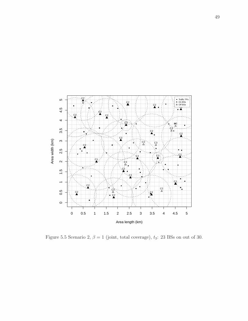
49

Area length (km)

Are

a w

idth

(km

)

0 0.5 1 1.5 2 2.5 3 3.5 4 4.5 5

00.

51

1.5

22.

53

3.5

44.

55

C

C

C

C

C

C

C

C

C

C

C

C

C

C

C

C

C

C

C

C

C

C

C

C

C

C

C

C

C

C

2

2

2

2

2

3

2

3

3

2

2

3

2

3

1

2

2

3

2

3

2

1

2

2

2

2

2

2

2

2


Figure 5.5 Scenario 2, β = 1 (joint, total coverage), t3: 23 BSs on out of 30.

50

Area length (km)

Are

a w

idth

(km

)

0 0.5 1 1.5 2 2.5 3 3.5 4 4.5 5

00.

51

1.5

22.

53

3.5

44.

55

C

C

C C

CC

C

CC

CC

C

CC

C

CC

C

C

C

C

C

C

C

C

C

C

C

C

C

C

C

C

C

C

C

2

2

3 2

21

2

32

23

2

22

2

32

2

2

2

3

3

3

3

3

3

2

3

1

3

2

3

2

3

2

2


Figure 5.6 Scenario 2, β = 1 (joint, partial coverage), t3: 6 BSs on out of 36.

51

deployed network, as soon as a TP switches from the idle to the active state, an additional

BS can be turned on to route the new provided traffic. The outcome of the partial coverage

approach, as called in Section 5.7.2, is displayed in Figure 5.6 for β = 1. Time period t3

has been represented to point out the great difference with the previous examples: here we

observe that only 6 BSs can serve the traffic requested by active users, but as much as 36 BSs

are installed to ensure the area full coverage. Note that, to further increase the operational

savings, the deployed network counts 6 more BSs than the topology obtained by using the

joint approach with the same value of β = 1 (Figures 5.4 and 5.5). With reference to the

joint optimization cases described above, where each TP had to lie in the coverage region of

an active BS, 31% of energy savings (β = 1) are expected if the partial coverage approach is

adopted, corresponding to almost 5250 ¤ spared every year; moreover, the percentage raises

to 61% when compared to the two-step total coverage approach depicted in Figure 5.2, which

is equivalent to 13250 ¤ yearly savings.

Tables 5.4 and 5.6 summarize the results obtained solving Scenario 2 with, respectively,

the total and partial coverage models, using different values of the trade-off parameter β.

Also, Tables 5.3 and 5.5 display the results for Scenario 1 in the same cases. The following

entries are reported:

1. The resolution time required by CPLEX to optimize the test instances;

2. CapEx, expressed in Euro and corresponding to the value of the first component of the

objective function;

3. OpEx for the whole network, calculated over a 8 year period by considering the Italian

energy cost for business users of 0.35 ¤ per kWh;

4. Number and type of BSs installed in the area;

5. Number of BSs powered on during every time period.

Percentages in parenthesis express the CapEx and energy consumption increase/decrease with

respect to the case when β = 0 and only capital costs are minimized. Moreover, Tables 5.5

and 5.6 include percentage variations in CapEx and OpEx with respect to the corresponding

examples in Table 5.3 and Table 5.4.

As already pointed out, increasing the value of β means increasing the installation costs as

well as the number of BSs, while decreasing the total energy consumed. The same behavior

can be observed for all test scenarios: taking as an example the results in Table 5.3, obtained

for Scenario 1 by applying the original joint model, the CapEx growth turns out to be 11%

with β = 1, 14% with β = 5 and 18% with β = 10 with respect to the two-step approach.

Power demand, on the other hand, decreases 55% when β = 1, 57% when β = 5 and 60% when

β = 10. With easy calculations, we found that when the trade-off parameter is set to 5, the

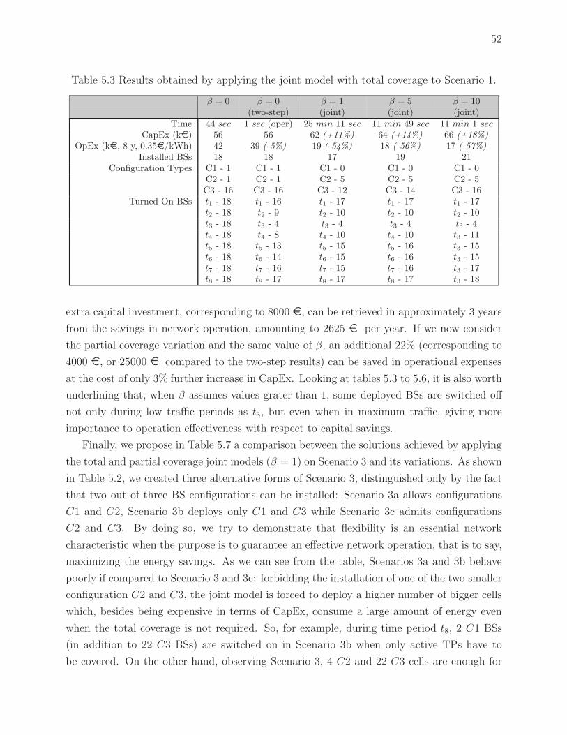
52

Table 5.3 Results obtained by applying the joint model with total coverage to Scenario 1.

β = 0 β = 0 β = 1 β = 5 β = 10(two-step) (joint) (joint) (joint)

Time 44 sec 1 sec (oper) 25 min 11 sec 11 min 49 sec 11 min 1 secCapEx (k¤) 56 56 62 (+11%) 64 (+14%) 66 (+18%)

OpEx (k¤, 8 y, 0.35¤/kWh) 42 39 (-5%) 19 (-54%) 18 (-56%) 17 (-57%)Installed BSs 18 18 17 19 21

Configuration Types C1 - 1 C1 - 1 C1 - 0 C1 - 0 C1 - 0C2 - 1 C2 - 1 C2 - 5 C2 - 5 C2 - 5C3 - 16 C3 - 16 C3 - 12 C3 - 14 C3 - 16

Turned On BSs t1 - 18 t1 - 16 t1 - 17 t1 - 17 t1 - 17t2 - 18 t2 - 9 t2 - 10 t2 - 10 t2 - 10t3 - 18 t3 - 4 t3 - 4 t3 - 4 t3 - 4t4 - 18 t4 - 8 t4 - 10 t4 - 10 t3 - 11t5 - 18 t5 - 13 t5 - 15 t5 - 16 t3 - 15t6 - 18 t6 - 14 t6 - 15 t6 - 16 t3 - 15t7 - 18 t7 - 16 t7 - 15 t7 - 16 t3 - 17t8 - 18 t8 - 17 t8 - 17 t8 - 17 t3 - 18

extra capital investment, corresponding to 8000 ¤, can be retrieved in approximately 3 years

from the savings in network operation, amounting to 2625 ¤ per year. If we now consider

the partial coverage variation and the same value of β, an additional 22% (corresponding to

4000 ¤, or 25000 ¤ compared to the two-step results) can be saved in operational expenses

at the cost of only 3% further increase in CapEx. Looking at tables 5.3 to 5.6, it is also worth

underlining that, when β assumes values grater than 1, some deployed BSs are switched off

not only during low traffic periods as t3, but even when in maximum traffic, giving more

importance to operation effectiveness with respect to capital savings.

Finally, we propose in Table 5.7 a comparison between the solutions achieved by applying

the total and partial coverage joint models (β = 1) on Scenario 3 and its variations. As shown

in Table 5.2, we created three alternative forms of Scenario 3, distinguished only by the fact

that two out of three BS configurations can be installed: Scenario 3a allows configurations

C1 and C2, Scenario 3b deploys only C1 and C3 while Scenario 3c admits configurations

C2 and C3. By doing so, we try to demonstrate that flexibility is an essential network

characteristic when the purpose is to guarantee an effective network operation, that is to say,

maximizing the energy savings. As we can see from the table, Scenarios 3a and 3b behave

poorly if compared to Scenario 3 and 3c: forbidding the installation of one of the two smaller

configuration C2 and C3, the joint model is forced to deploy a higher number of bigger cells

which, besides being expensive in terms of CapEx, consume a large amount of energy even

when the total coverage is not required. So, for example, during time period t8, 2 C1 BSs

(in addition to 22 C3 BSs) are switched on in Scenario 3b when only active TPs have to

be covered. On the other hand, observing Scenario 3, 4 C2 and 22 C3 cells are enough for

53

Table 5.4 Results obtained by applying the joint model with total coverage to Scenario 2.


Time 25 sec 1 sec (oper) 1 min 51 sec 1 min 7 sec 19 secCapEx (k¤) 267 267 277 (+4%) 298 (+12%) 299 (+12%)

OpEx (k¤, 8 y, 0,35¤/kWh) 203 198 (-3%) 134 (-34%) 115 (-43%) 115 (-43%)Installed BSs 23 23 30 33 34



Table 5.5 Results obtained by applying the joint model with partial coverage to Scenario 1.



Vs. Total Coverage +0% +0% +0% +3% +0%OpEx (k¤, 8 y, 0.35¤/kWh) 42 33 (-21%) 16 (-62%) 14 (-67%) 13 (-69%)

Vs. Total Coverage -0% -15% -16% -22% -24%Installed BSs 18 18 17 21 21



54

Table 5.6 Results obtained by applying the joint model with partial coverage to Scenario 2.



Vs. Total Coverage +0% +0% +1% +14% +21%OpEx (k¤, 8 y, 0.35¤/kWh) 203 175 (-13%) 92 (-54%) 75 (-63%) 73 (-64%)

Vs. Total Coverage -0% -12% -31% -35% -37%Installed BSs 23 23 36 37 39



Table 5.7 Significative results obtained applying joint model with total and partial coverage(β = 1) to Scenario 3 and its variations.

Scenario 3 Scenario 3a Scenario 3b Scenario 3cTotal Coverage:

CapEx (k¤) 136 240 (+76%) 190 (+40%) 137 (+0.7%)OpEx (k¤, 8 y, 0.35¤/kWh) 46 71 (+54%) 197 (+328%) 46 (+0%)

Installed BSs C1 - 0 C1 - 0 C1 - 6 C1 - n.a.C2 - 12 C2 - 24 C2 - n.a. C2 - 12C3 - 16 C3 - n.a. C3 - 10 C3 - 17

Turned On BSs in t3 C1 - 0 C1 - 0 C1 - 6 C1 - n.a.C2 - 12 C2 - 14 C2 - n.a. C2 - 12C3 - 5 C3 - n.a. C3 - 2 C3 - 5


Partial Coverage:CapEx (k¤) 144 240 (+67%) 208 (+44%) 141 (-2%)

OpEx (k¤, 8 y, 0.35¤/kWh) 16 50 (+213%) 56 (+250%) 15 (-6%)Installed BSs C1 - 0 C1 - 0 C1 - 6 C1 - n.a.

C2 - 12 C2 - 24 C2 - n.a. C2 - 12C3 - 24 C3 - n.a. C3 - 28 C3 - 21



55

serving the traffic provided by TPs in the busiest period, decreasing power consumption at

almost one-fourth compared to the previous case. Similar results (but setting β = 10) are

represented in Figures 5.9 and 5.10, while Figures 5.7 and 5.8 report the network topology

obtained when the total area coverage is needed at all time.

5.8 Conclusion

Managing the network operation to follow traffic variations is certainly one of the most power-

ful instruments in mobile operator hands to reduce energy consumption, and so, operational

costs. By proposing an optimization framework that selects the BSs to be installed and

jointly switches them on and off according to the changing traffic load, in this paper we

strove to demonstrate that for the power management to be truly effective networks have to

be designed taking into account operational management.

The goal of our approach is not only to minimize both installation and operational costs,

but also to find the best trade-off between keeping low initial investments and reducing energy

consumption. Varying the trade-off parameter β between CapEx and OpEx, we got network

topologies with different characteristics. Networks with a low installation cost are not very

efficient from an energy consumption standpoint since those tend to use mostly big cells. On

the other hand, the most energy efficient networks include not only small cells with low energy

consumption, but also some bigger cells to provide the energy management mechanism with

enough flexibility to adapt the network capacity in different time periods.

Future work will consider heuristic methods for very large scale network instances and

the development of real-time on-line operation models incorporating user mobility.

56

Area length (km)

Are

a w

idth

(km

)

0 0.5 1 1.5 2 2.5 3 3.5 4

00.

51

1.5

22.

53

3.5

4

C

CC

C

C

C

C

C

C

C

C

C

C

C

C

C

C

CC

C

C

C

C

C

C

C

C

C

C

3

22

2

3

2

3

2

2

3

3

2

3

3

3

3

2

33

2

3

3

2

3

2

3

3

2

3


Figure 5.7 Scenario 3, β = 10 (joint, total coverage), t3.

57

Area length (km)

Are

a w

idth

(km

)

0 0.5 1 1.5 2 2.5 3 3.5 4

00.

51

1.5

22.

53

3.5

4

C

C

C

C

CC

C

CC

C

C

CC

C

C

C

3

3

3

3

13

1

11

3

1

33

3

1

3


Figure 5.8 Scenario 3b, β = 10 (joint, total coverage), t3.

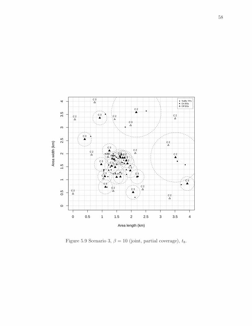
58

Area length (km)

Are

a w

idth

(km

)

0 0.5 1 1.5 2 2.5 3 3.5 4

00.

51

1.5

22.

53

3.5

4 C

C

C

C

C

C

C

C

C

C

C

C

C

C

C

C

C

C

C

C

C

C

C

C

C

C

C

C

C

C

C

C

C

C

C

C

C

C

3

2

2

3

2

3

3

2

2

3

3

3

2

3

3

2

3

3

3

3

3

3

3

3

3

3

3

2

3

2

3

3

3

2

3

2

2

3


Figure 5.9 Scenario 3, β = 10 (joint, partial coverage), t8.

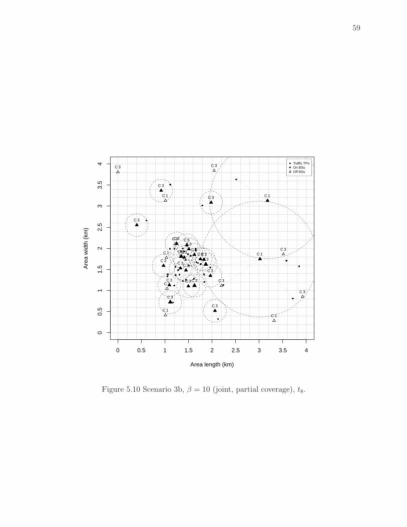
59

Area length (km)

Are

a w

idth

(km

)

0 0.5 1 1.5 2 2.5 3 3.5 4

00.

51

1.5

22.

53

3.5

4

C

C

C

CC

C

C

C

C

CCC

C

C

C

C

C

C

C

C

C

C

C

C

C

C

C

C

CC

C

CC

C

3

3

3

33

3

3

3

3

133

1

3

1

3

3

3

3

3

1

3

3

3

3

3

3

1

33

3

33

1


Figure 5.10 Scenario 3b, β = 10 (joint, partial coverage), t8.

60

CHAPTER 6

ARTICLE 3: JOINT DESIGN AND MANAGEMENT OF ENERGY-AWARE

MESH NETWORKS


Published on Ad Hoc Networks, April 2012

6.1 Abstract

This paper deals with the joint planning and energy management operation of wireless mesh

networks. We claim that energy management should be incorporated at the planning stages

to produce an effective energy-management operation. For this, we propose a mathematical

framework that takes into account the trade-off of capital expenditures versus energy-related

operational ones when designing the network. We also present results that put into relevance

the impact of different coverage policies on energy efficiency.

6.2 Introduction

The debate on global warming and energy efficiency in ICT is becoming increasingly im-

portant. There is now evidence (The Climate Group, 2008), that the ICT industry has a

significant part of responsibility for the global carbon emissions, with telecommunications

networks (including mobile, WLANs, LANs and wired networks) representing almost 50% of

ICT power expenditures (Koutitas and Demestichas, 2010).

The answer of the research community has been green networking, consisting on a new

way of building and managing telecommunications networks to reduce their energy needs.

As a matter of fact, it is clear that working towards the so-called green networks is not only

profitable in terms of the cost savings related to power expenses (OpEx, operational and man-

agement expenditures), but also allows the deployment of networks having low environmental

impact.

Among the network segments, the access is the one with the major influence on en-

ergy consumption, being liable for 80% of the overall power expenditures (Gruber et al.,

2009; Koutitas and Demestichas, 2010). This is mostly because WANs (WANs) are usually

dimensioned to satisfy the quality constraints under peak traffic conditions, resulting in over-

provisioning in low-demand periods thus wasting a significant amount of power. From this

61

point of view, trying to minimize the energy consumption of deployed access elements (that

is to say, base stationss) is an important goal.

There has been interesting models and approaches to deal with the problem of power

savings in both wireless and wired networks (Mellah and Sanso, 2009). Nevertheless, a

fundamental issue that has been overlooked is that an effective energy-aware operation is

closely dependent on the planning decisions taken during the network design phase. In other

words, we claim that when the network is designed with the classical cost-performance trade-

off, the energy management operation would be less efficient than if energy management is

directly incorporated at the planning stages. To the best of our knowledge, the only example

of this kind of analysis can be found in our previous work Boiardi et al. (2010), where the

significant advantages of jointly optimizing network design and operation in cellular networks

are evaluated.

Differently from Boiardi et al. (2010), we focus here on wireless mesh networks (WMNs), a

newly emerged type of access network offering wireless connectivity with the use of cheap and

low transmission power devices. WMNs are dynamically self-organized and self-configured

communication infrastructures, with a high degree of cooperation between many individual

wireless stations. Each node works not only as a host but also as a router, forwarding

packets on behalf of other nodes that may not be within direct transmission range of their

destinations. Thus, the nodes automatically establish mesh connectivity among themselves,

creating in effect an ad hoc network (Akyildiz et al., 2005). However, as usually happens in the

other types of access networks, WMNs infrastructure devices are always active. Thus, during

lower traffic periods the energy consumption is the same as in busy hours, while it would

be possible to save a large amount of power by turning off unnecessary nodes. Concerning

this issue, an energy-aware approach for such kind of networks was tackled in Capone et al.

(2012b), where the power expenses of a deployed network were minimized by dynamically

selecting a subset of base stationss to be switched on. However, that article did not consider

energy management jointly with network planning but as a purely operational feature.

The question that we want to answer in this paper is, given the highly adaptive features

of mesh networks, to what extend the philosophy of jointly planning and energy optimization

yields important energy efficient results. For this, we will proceed to present a mathematical

framework and extensive results to seize the advantage of this type of approach for Wireless

Mesh green networking.

The reminder of the paper is structured as follows. In Section 6.3 we present an overview

on related work. Section 6.4 provides a description of the Wireless Mesh system and gives an

overview of planning and operational models that are important preliminaries to understand

the joint optimization framework that is presented in Section 6.5. The resolution approach

62

is presented in Section 6.6, where we also explain the model variations used for testing

the effectiveness of our optimization method. Numerical results are fully commented in

Section 6.7, while Section 6.8 concludes the paper.

6.3 Related work

Several studies on green networking have appeared in the last few years, starting from the

seminal work of Gupta and Singh (2003). A complete overview of the main research ideas on

this topic can be found in Minami and Morikawa (2008) and Mellah and Sanso (2009), where

the authors survey different proposals for reducing the power consumption in both wired and

wireless networks.

Despite the fact that wireless systems have high responsibility in the increase of power

expenditures, most of the work on infrastructure consumption have focused on wired net-

works. However, wireless research has always been involved in energy-related problems given

the mobile nature of the network devices that is pushing for improvements in batteries life

and coverage techniques. Therefore, the literature includes many studies on energy-efficient

devices (Zhang et al., 2006; Louhi, 2007) and protocols (Jones et al., 2001) for WLANs and

cellular networks (for an excellent review, see Karl et al. (2003)). On the other hand, the

interest in infrastructure wireless green networking design and operation has only started in

recent years and deals more with management than with planning issues.

For instance, concerning WLANs, in Jardosh et al. (2007) and Jardosh et al. (2009) the

resource on demand (RoD) approach is proposed, aiming at powering off some access points

during off-peak traffic periods following real-time traffic variations or fixed pre-determined

schedules. The system behavior under two different RoD strategies is evaluated in Marsan

et al. (2010). Considering cellular networks, several works assess the possibility of switching

off some nodes when they are underutilized, based on average measurements of traffic ex-

change between nodes (Chiaraviglio et al., 2008b) or deterministic traffic variations during

the day (Marsan et al., 2009). In our previous work Boiardi et al. (2010), for the first time the

energy expenses problem is tackled from a dual standpoint: given that an effective energy-

aware network operation closely depends on the locations chosen for the network devices, we

develop a joint design and management model that aims at limiting both energy consumption

and operational expenditures.

Concerning WMNs in general, previous work concentrates mainly on MAC and routing

protocols, mobility management and security topics. Most of the time, the network topology

(that is to say, the positions of routers and gateways) was pre-established and the goal was to

optimize the routing or the channel assignment. Few authors have investigated the problem

63

of planning wireless mesh access networks. In Wang et al. (2007), a single pre-installed access

point is considered and only the positions of routers are optimized, while in Qiu et al. (2004)

and He et al. (2007) the authors formulate a modeling approach for locating gateways given

the locations of the other nodes. A mathematical model for the complete WMN design

is proposed in Amaldi et al. (2008), where the number and positions of mesh routers and

access points are to be selected, always taking into account typical network issues such as

traffic routing and channel assignment. In the context of green networking, an energy-aware

management for WMNs is obtained in Capone et al. (2012b) where starting from a previously

deployed network, the authors try to minimize the power consumption in a time varying

context by dynamically turning on and off some base stations (routers or access points) (see

Section 6.4.3 for more details on the models presented in Amaldi et al., 2008; Capone et al.,

2012b).

A very interesting framework is presented in Chen et al. (2011) where four fundamental

trade-offs for an effective green network are stated and an excellent overview of the current

and future studies in green networking research area is presented. Moreover, the exhaustive

analysis of the Deployment Efficiency - Energy Efficiency (DE-EE) trade-off reported in Chen

and Tsai (2010) is a good starting point to better understand the importance and complexity

of the issue we tackle in this paper.

Differently from the aforementioned papers, we present the following original contribu-

tions:

• We propose the joint optimization of the planning and energy-aware operation for

wireless mesh networks and create, for the first time, a rigorous optimization model.

• We compare the savings obtained with the joint planning and operation framework phi-

losophy with the one obtained when planning and energy aware operation are performed

in separate stages.

• We compare the energy savings obtained for Mesh and cellular networks obtained with

the same type of modeling philosophy.

• We study the effect of different planning and operating coverage strategies on overall

network consumption.

6.4 System description and preliminary mathematical models

The philosophy of the modeling framework that will be presented in Section 6.5 is based

on exploiting the dynamic features of WMNs to design a system that is not only cost-

effective, but also follows the demand in an energy-efficient way during normal operation.

64

In order to follow the demand, we must first characterize it by time periods and the energy

management framework will consist in deciding which device should be put down during the

daily operation to minimize energy consumption. As the model is jointly a planning and an

operational one, the framework idea is to choose, at the same time, the network configuration

and the operational features.

In the rest of this Section, we first provide an overview of the WMN system description.

Next, we discuss how traffic variations are characterized. The last subsection is devoted to

revisiting the planning and operational models that have been previously presented and that

are necessary to understand our joint planning and operation proposal of Section 6.5.

6.4.1 System description

wireless mesh networks are made up of two types of fixed elements, mesh routers (MRs) and

mesh access points (MAPs), forming the mesh backbone for mobile users, named mesh clients

(MCs). From now on, when generally referring to MRs and MAPs the term base stations

(BSs) will be used. Both kinds of BSs have the task of setting up a wireless distribution

system (WDS) by connecting to other mesh routers and access points through point to point

wireless links while providing network access for the MCs. In addition, MAPs, representing

only a restricted set of routers, behave as gateways toward the wired backbone, enabling the

integration of WMNs with other networks (typically the Internet).

In developing our WDS, we follow the assumptions made in Capone et al. (2012b). MRs

and MAPs that reside in the respective covering ray can communicate through dedicated

wireless channels, each one having bidirectional capacity unvarying with the distance. We

admit that the traffic in a link does not affect closer links since all devices are equipped with

multiple network interfaces. Concerning MCs, they can be assigned to a BS only if they are

included in a circular cell centered in the BS and having a ray of 250m. Moreover, mesh users

are served by the nearest active router and are connected to the Internet through multi-hop

communications.

In terms of numerical values, we use the Wi-Fi 802.11n standard for communication

between routing devices, with a nominal link capacity of 450Mbps and a coverage ray of

450m. Note that the coverage ray between two BSs is almost doubled with respect to the

one between BSs and MCs since directive antennas are used for connecting MRs and MAPs

in order to limit unwanted interference. Finally, the access technology Wi-Fi 802.11g with

54Mbps is chosen, shared among all users assigned to a BS.

65

6.4.2 Traffic variations pattern

Different studies have dealt with traffic variations measurement in wireless access networks (Pries

et al., 2009; Heegaard, 2007). Considering an approximated traffic profile based on these stud-

ies, in Lorincz et al. (2010); Boiardi et al. (2010); Capone et al. (2012b) the authors split

the whole day into time periods in order to take into account the demand fluctuations in

WLANs, cellular or mesh networks, respectively. By dividing the day into smaller intervals

in which users behavior is assumed unchanged, the on-off operation of the access network will

allow following the traffic variations and reducing power consumption of unneeded devices.

Let T be the ordered set of time periods displayed in Table 6.1. Note that no time gap

is admitted between adjacent intervals, and the summed duration of all intervals is equal to

the number of hours in a day. A value ρt is assigned to each time period, representing the

probability that an MC provides traffic to the network. In other words, ρt is the percentage

of active users typical of every time interval.

As presented in Capone et al. (2012b), two different degrees of congestion have been

tested:

- Standard profile, in which active MCs provide a traffic amount randomly generated

between 1 and 10Mbps;

- Busy profile, in which the demand of active users varies from 8 to 10Mbps.

6.4.3 Basic approaches to network planning and energy management

Before introducing our joint network design and management model (in Section 6.5) we

briefly present the two mathematical programming models representing the basic approaches

to the separate problems of WMN planning (Amaldi et al., 2008) and WMN energy manage-

ment (Capone et al., 2012b). Note that the original notation was changed for commonality

in model description.

WMN planning

The general idea of the formulation presented in Amaldi et al. (2008) is deciding where and

what kind of access devices should be installed in order to satisfy the users demand and

minimize CapEx costs. Let S be the set of candidate sites (CSs) available to host a MR or

a MAP and let I be the set of MCs, each one providing a constant traffic value defined by

di, i ∈ I. Let N be a special node representing the Internet. Moreover, the set J(i)h is required

to recognize the most convenient BSs for every MCs: it represents the subset of BSs covering

user i, ordered by decreasing received power.

66

Table 6.1 Time periods and demand variations during a day.

Index 1 2 3 4 5 6 7 8

Start 00:00 3:00 6:00 9:00 12:00 15:00 18:00 21:00End 3:00 6:00 9:00 12:00 15:00 18:00 21:00 24:00

Duration 3 h 3 h 3 h 3 h 3 h 3 h 3 h 3 hρt 0.35 0.1 0.45 1 0.7 0.85 0.6 0.5

Two are the required binary parameters: aij is equal to 1 if MC i is covered by the BS

located in site j, while bjl is equal to 1 if a wireless link can be installed between the BSs in

sites j and l.

The binary decision variables xij are used to assign MC i to the BS located in j, the

installation variables zj indicate wether CS j is chosen in the solution, variables wj show if a

MAP is installed in site j and variables kjl define if the BSs located in j and l are connected

through a wireless link. Additional integer variables fjl represent the traffic on wireless link

(j, l), while fjN is the flow from the MAP in site j to the Internet.

The mathematical model of the WMN design problem is the following:

min∑

j∈S

(zjγj + pjwj) (6.1)

subject to:∑

j∈S

xij = 1 ∀i ∈ I (6.2)

xij ≤ aijzj ∀i ∈ I, j ∈ S (6.3)∑

l∈S

(flj − fjl) +∑

i∈I

dixij = fjN ∀j ∈ S (6.4)

flj + fjl ≤ ujlkjl ∀j, l ∈ S (6.5)

fjN ≤ mwj ∀j ∈ S (6.6)∑

i∈I

xijdi ≤ cj ∀j ∈ S (6.7)

kjl ≤ zj , kjl ≤ zl ∀j, l ∈ S (6.8)

kjl ≤ bjl ∀j, l ∈ S (6.9)

zJ(i)l

+

li∑

h=l+1

xiJ

(i)l

≤ 1 ∀i ∈ I, l : 1...Bi − 1 (6.10)

xij , zj , kjl, wj ∈ {0, 1} ∀i ∈ I, j, l ∈ S (6.11)

Objective function (6.1) minimizes the network deployment costs, given by a basic installation

cost γj common to all BSs located and additional costs pj due to the connection of MAPs

67

to the Internet. Constraints (6.2) and (6.3) insure that each MC is assigned to a BS that

covers it. (6.4) are flow balance equations, while (6.5), (6.6) and (6.7) are capacity constraints

for links, MRs and MAPs respectively. Constraints (6.8) and (6.9) guarantee that a link is

installed only if the two involved nodes are both active and neighbors, while (6.10) force the

assignment of every MC to the nearest installed BS. Finally, constraints (6.11) impose binary

values for some decision variables.

Notably, this formulation does not take into account any network operation or energetic

aspect and no demand variations over time are considered. These will be taken into account

in the next subsection.

WMN energy management

The model revisited here was formulated in Capone et al. (2012b). Given an existing network,

the problem is that of deciding which BSs should be switched off according to the variations

of the users traffic profiles. In addition to the two sets previously defined, let T be the set of

time intervals described in Table 6.1 and let G ⊆ S the subset of BSs that are MAPs.

Since the traffic offered by users is different depending on the time intervals, an extended

traffic matrix dit is defined. The assignment of MCs can now change in time, so that decision

variables x, f and fN are now identified by one more index t. Another group of variables,

yjt, is introduced to indicate if the BS located in j is active at time t.

The WMNs energy management formulation is the following:

min∑

j∈S

∑

t∈T

ǫjzjt∆(t) (6.12)

subject to:∑

j∈S

xijt = 1 ∀i ∈ I, t ∈ T (6.13)

xijt ≤ aijzjt ∀i ∈ I, j ∈ S, t ∈ T (6.14)∑

l∈S

(fljt − fjlt) +∑

i∈I

ditxijt = fjNt ∀j ∈ S, t ∈ T (6.15)

fljt + fjlt ≤ ujlbjlzjt ∀j, l ∈ S, t ∈ T (6.16)

fjNt ≤ m ∀j ∈ S, t ∈ T (6.17)∑

i∈I

xijdi ≤ cj ∀j ∈ S, t ∈ T (6.18)

zJ(i)l

+

li∑

h=l+1

xiJ

(i)l

≤ 1 ∀i ∈ I, l : 1...Bi − 1 (6.19)

xij , zj ∈ {0, 1} ∀i ∈ I, j, l ∈ S (6.20)

68

Here the objective function (6.12) aims at minimizing the sum of BSs energy consumption ǫj

over all time periods. As for the previously described model, (6.13) and (6.14) are assignment

constraints, (6.15) are flow balance constraints and (6.16), (6.17) and (6.18) are capacity

constraints for links, MAPs Internet access and BSs. Finally, constraints (6.19) guarantee

the best possible assignment for every user. Constraints (6.20) impose binary values to the

decision variables.

6.5 Joint network design and management for Wireless Mesh Networks

In the previous Section, we revisited, respectively, a planning and energy management model

for WMNs. In this Section, we present a joint planning and management optimization

approach based on the modeling philosophy proposed in Boiardi et al. (2010) for cellular

networks that combines the minimization of installation costs and the maximization of energy

savings. This way we strive to underline the tight relationship existing between an effective

energy-aware network operation and wise decisions made during planning phases. We now

present the notational framework, a reference model as well as some key relaxations that will

be used for comparison purposes in the results section.

6.5.1 Notational framework

To be able to set the mathematical model, we need an additional notation. For the sake of

completeness, some of the notation that was first presented in Section 6.4.3 is also included

here.

Sets

I : Set of MCs generating variable traffic;

S : Set of the available CSs for the BSs;

T : Set of time intervals;

J(i)h : Subset of BSs covering MC i, ordered by descending received power.

Parameters

dit : Traffic provided by MC i in period t;

cj : Access capacity of the BS located in site j;

ujl : Capacity of the wireless link between BSs located in sites j and l;

m : Capacity of the MAPs Internet access;

γj : Installation cost for a MR located in site j;

69

pj : Installation cost for a MAP located in site j (it includes the cost for connecting the

MAP with the wired backbone);

ǫj : Power consumption for a MR located in site j;

ψj : Power consumption for a MAP located in site j;

Bi : Number of BSs covering MC i;

∆(t) : Duration of time period t;

β : Weight parameter used for trading-off the objective function.

aij : Equal to 1 if MC i is covered by a BS installed in j, 0 otherwise;

bjl : Equal to 1 if a wireless link between BSs located in sites j and l is possible, 0 otherwise.

Variables

zj =

1 if a MR is installed in site j,

0 otherwise;(6.21)

wj =

1 if a MAP is installed in site j,

0 otherwise;(6.22)

yjt =

1 if the MR installed in site j is active in period t,

0 otherwise;(6.23)

rjt =

1 if the MAP installed in site j is active in period t,

0 otherwise;(6.24)

xijt =

1 if MC i is assigned to a BS installed in site j

in period t,

0 otherwise;

(6.25)

kjl =

1 if there is a wireless link between the BSs in

sites j and l,

0 otherwise;

(6.26)

fjlt : Flow between BSs located in sites j and l in time t;

fjNt : Flow between MAP located in site j and Internet (N) in time t.

70

6.5.2 The reference model

The first joint network design and management problem for WMNs will be called (P0) and

it is defined as follows:

The objective function

min β∑

j∈S

(zjγj + pjwj) + (1− β)∑

j∈S

∑

t∈T

(ǫjyjt + ψjrjt)∆(t) (6.27)

The objective function is composed of two terms. The first one represents the installation

costs of MRs and MAPs in selected CSs (CapEx), while the second one accounts for the

power consumption of the active devices in any time interval (OpEx). The parameter β,

which varies in the [0, 1] interval, represents the trade-off between the two components, as it

changes the importance given to the OpEx with respect to the CapEx. Starting from β = 1,

when just capital expenses are minimized, we will gradually reach the opposite case of β = 0

(minimization of power costs only) after evaluating individual values. Then, comparing the

intermediate results with the two extreme cases, we will be able to underline the benefits of

our approach and show how both network planning and management can be wisely improved

by considering them in a joint fashion.

Assignment constraints

∑

j∈S

xijt = 1 ∀i ∈ I, t ∈ T (6.28)

xijt ≤ aij(yjt + rjt) ∀i ∈ I, j ∈ S, t ∈ T (6.29)

Two different assignment constraints are needed. Equations (6.28) impose that every MC is

assigned to one and only one BS. Constraints (6.29) assign every MC only to a BS that is

active and that covers it.

Installation constraints

zj + wj ≤ 1 ∀j ∈ S (6.30)

Installation constraints (6.30) guarantee that at most one device (MR or MAP) is installed

in every CS.

71

Activation constraints

yjt ≤ zj ∀j ∈ S, t ∈ T (6.31)

rjt ≤ wj ∀j ∈ S, t ∈ T (6.32)

These constraints allow the activation of a MR (6.31) or a MAP (6.32) in any time period

only if the device has been installed.

Flow conservation constraints

∑

l∈S


i∈I

ditxijt = fjNt ∀j ∈ S, t ∈ T (6.33)

Constraints (6.33) define the flow balance in site j. The term∑

l∈S fljt is the total traffic

received by j from neighboring sites,∑

l∈S fjlt is the total traffic transmitted by j to neigh-

boring sites,∑

l∈i ditxijt is the traffic related to the users assigned to j and fjNt is the traffic

transmitted to the wired backbone.

Capacity constraints

∑

i∈I

xijtdit ≤ cj(yjt + rjt) ∀j ∈ S, t ∈ T (6.34)

fljt + fjlt ≤ ujlkjl ∀j, l ∈ S, t ∈ T (6.35)

There are two different groups of capacity constraints. (6.34) insures that the total traffic

demand of the MCs assigned to a BS does not exceed the BS capacity, while constraints

(6.35) refer to the maximum capacity available for existing links.

Link use constraints

fljt + fjlt ≤ ujl(yjt + rjt) ∀j, l ∈ S, t ∈ T (6.36)

fljt + fjlt ≤ ujl(ylt + rlt) ∀j, l ∈ S, t ∈ T (6.37)

fjNt ≤ mrjt ∀j ∈ S, t ∈ T (6.38)

Constraints (6.36) and (6.37) allow the use of the link (l, j) only in the case BSs in j and l

are turned on. Equations (6.38) state that the capacity of the MAPs Internet access must

72

not exceed m, while forcing the flow toward the backbone to zero if the device in j is not a

gateway.

Link existence constraints

kjl ≤ zj + wj ∀j, l ∈ S (6.39)

kjl ≤ zl + wl ∀j, l ∈ S (6.40)

kjl ≤ bjl ∀j, l ∈ S (6.41)

The three constraints above allow the existence of a wireless link between two BSs only if

they are both active ((6.39) and (6.40)) and neighbors (6.41).

Best power constraints

yJ(i)l

t+ r

J(i)l

t+

li∑

h=l+1

xiJ

(i)l

t≤ 1 ∀i ∈ I, t ∈ T, l : 1...Bi − 1 (6.42)

Constraints (6.42) force the assignment of every MC to the most convenient BS, according

to a proper parameter such as the received signal strength.

Binary constraints

xijt ∈ {0, 1} ∀i ∈ I, j ∈ S, t ∈ T (6.43)

yjt, rjt ∈ {0, 1} ∀j ∈ S, t ∈ T (6.44)

zj , wj ∈ {0, 1} ∀j ∈ S (6.45)

kjl ∈ {0, 1} ∀j, l ∈ S (6.46)

Finally, binary constraints impose binary values to some of the decision variables.

6.5.3 The partial covering-relaxed problem

In order to underline the importance of our study and compare the results in different sit-

uations, we have also developed a relaxed variation of the reference model. Just like (P0),

the Partial Covering-Relaxed Problem (P1) aims at providing a full-coverage network deploy-

ment, but in this case our objective is that of guaranteeing network services only to those

73

clients that are active in any time period: in this way, those BSs that have only inactive users

in their covering ray can be turned off.

For this purpose, we need to introduce a new set of binary parameters hit that is equal to

1 if the MC i is providing traffic in time period t. Then, in order to limit the network service

only to active users, constraints (6.28) of (P0) should be replaced by:

hitxijt ≤ aij(yjt + rjt) ∀i ∈ I, j ∈ S, t ∈ T (6.47)

(P1) can then be written as:

min (6.27)

subject to: (6.28), (6.47), (6.30)− (6.46).

6.6 Resolution approach

The proposed mathematical model has been developed using the AMPL programming lan-

guage and optimized with the CPLEX solver.

Realistic mesh network instances have been generated modifying the IG proposed in Capone

et al. (2012b). The main features of the IG are given below.

6.6.1 Instance Generator and input assumptions

Since our model generates a network topology and manages network operation, the main

task of the IG is to randomly place CSs and users location in the analyzed area. Also, for

each client, the instance generator computes two random traffic values in each time interval,

according to the different congestion levels presented in Section 6.4.2. Then, for every pair

of MC and CS, it computes the mutual distance and sets the corresponding value of aij to 1

if user i is in the coverage ray of the BS that could be installed in j. The same operation is

done for each couple of CSs, in order to verify if a wireless link is possible between them and

set the corresponding parameters bjl to the correct values.

In order to produce factual mesh network instances, some IG input parameters referring

to BSs features and derived from real field tests were set to the following values:

- Covering ray for communications between BSs: 450m;

- Covering ray for communications between a BS and a MC: 250m;

- Capacity ujl of the wireless link connecting two BSs located in j and l, ∀j, l ∈ S:

300Mb/s;

- Capacity m of MAPs Internet access: 10Gb/s;

74

- Access capacity cj for a BS located in j, ∀j ∈ S: 40Mb/s;

- Installation cost γj for a MR located in j, ∀j ∈ S: 200 ¤;

- Installation cost pj for a MAP located in j, ∀j ∈ S: 400 ¤;

- Power consumption ǫj for a MR located in j, ∀j ∈ S: 15W ;

- Power consumption ψj for a MAP located in j, ∀j ∈ S: 18W .

Moreover, specific control parameters are added to the random generation to guarantee the

network feasibility. Also note that in our tests,we assume that the power consumed by MRs

and MAPs do not vary with link utilization, which, depending on the type of equipment,

may be a reasonable assumption.

6.6.2 Test scenarios

With the help of the IG three different WMN test scenarios were generated. Their features

are described in Table 6.2. The first column reports the name that will be used to identify

the instance. The second entry represents the area size (expressed in squared meters) and

the next is the number of CSs available in the area. The last column presents the number of

users placed in the area.

As introduced in Section 6.4.2, we considered two different traffic profiles for every test

scenario. In both situations, during time period t only a percentage ρt of users provides traffic

to the network. When the standard profile is considered, the traffic value related to each MC

is randomly chosen by the IG between 1 and 10Mb/s, while the same value ranges from 8

to 10Mb/s in the case of busy profile.

6.6.3 Additional tests and variations

To underline the effectiveness of our results, we introduce three other possible variations of

the problem.

Variable capacity for backbone wireless links

As reported in subsection 6.6.1, in our tests we use a fixed capacity uij of 300 Mb/s for

wireless links connecting two BSs, provided that they are no more than 450 m away. In order

Table 6.2 Characteristics of the WMN test scenarios.

WMN Size Area Size (m2) CSs Number MCs Number

Small 1000×1000 16 60Medium 1500×1500 40 130

Large 2500×2500 64 240

75

to verify the soundness of our assumption, we have also created a set of experience that sets

different values of link capacity depending on the BSs mutual distance:

- Distance up to 60 m from BS i to BS j: uij = 300Mb/s;

- Distance 60 m—120 m from BS i to BS j: uij = 240Mb/s;



- Distance 300 m—450 m from BS i to BS j: uij = 60Mb/s.

Thus, our purpose is to demonstrate that no substantial variation in CapEx and OpEx

values, as well as in the network design and management, appears when the fixed capacity

assumption is adopted.

The cellular comparison

Here we assume that no router can be installed so that each CS can host only a gateway

(MAP). This case represents a cellular network where every base station behaves as a gate-

way, being directly connected to the backbone and routing the traffic towards the Internet

without the help of other nodes. This MAPs only scenario aims at sizing the energy savings

that can be obtained if a multi-hop mesh network is deployed instead of a cellular one.

The two-step approach

In the third test, the energy management model proposed in Capone et al. (2012b) and

reported in Section 6.4.3 is applied to a pre-computed network design. Differently from the

network planning considered in Capone et al. (2012b), this is directly obtained from the

model we propose by setting the weight parameter β to 1, so it is optimized to get the

minimum capital expenses. This kind of approach can be identified as a two-step approach,

since the network design is computed first and only then an energy management model can

be applied to the network. Thus, by comparing our joint model results with the ones given

by the two-step optimization, we strive to show the effects of a combined approach on the

network deployment and the benefits on energy savings.

The relaxed two-step approach

Finally, we test a different version of the two-step procedure described above where the energy

management is executed by considering only the active MCs. In this last case, the model

presented in Section 6.4.3 is modified by excluding constraints (6.14) and setting the value of

the summation in constraints (6.13) equal to hit. We refer to Capone et al. (2012b) for more

76

details on the adopted relaxing technique. This relaxed two-step approach will be compared

with the results obtained by our problem (P1).

6.7 Numerical results

In this Section, we present selected results from a large set of instances for Problems (P0),

(P1) and its variations.

6.7.1 Savings obtained using the reference model

This subsection is devoted to the presentation of summary results as well as more detailed

results concerning the application of the basic planning and operation problem (P0).

Summary results

For every scenario, we tested different values of β to see the effect of giving more weight to

the operational and energetic aspect of the network.

Table 6.3 provides an overview of the percentage of energy savings that can be obtained

by exploiting the joint design and management model (P0). Each entry refers to a particular

value of β applied to the previously described test scenarios . The percentages are calculated

with respect to the energy requirement of the same test scenarios when β is set to 1. In

fact, when β = 1 no energy saving operational considerations are taken into account and the

model provides a simple network design optimization. As a result, all the installed BSs are

constantly turned on and no energy management mechanism is enabled.

One can observe from the values in the table that by just setting β to 0.8, which enables

the energy management term of the objective function, the energy consumption during the

day decreases by more than 30% in the best situations. These reductions are due to the fact

that, when the weight parameter is smaller than 1, our joint approach is pushed to optimize

not only the topology but also the operation of the considered network. Therefore, only those

BSs that are required for routing the MCs’ traffic or guaranteeing the total area coverage are

Table 6.3 Comparison of energy saving percentages obtained from (P0) in all test scenarios(percentages are referred to the cases of β = 1).

Small Small Medium Medium Large LargeStandard Busy Standard Busy Standard Busy

β = 0.8 20.49% 29.32% 12.39% 32.11% 17.94% 25.51%β = 0.5 27.66% 29.32% 14.98% 32.11% 20.80% 28.01%β = 0.1 27.66% 30.09% 20.87% 32.67% 23.11% 28.84%

77

turned on, while the others can be powered off. Further decreases of β lead to low decreases

of the energy consumption in the busy version of all the test scenarios, while better results

come from the cases with standard traffic. This difference in the network behavior is clearly

caused by a higher amount of traffic that has to be managed in the busy profile cases.

Detailed results

Some detailed results on energy efficiency, costs and energy management can be found in

Table 6.4, that shows more clearly how (P0) behaves when applied to the largest test sce-

nario. The rows of the table display, respectively, the values of capital expenditures (CapEx,

expressed in Euro), the energy requirements during the day (expressed in Wh), the daily

energy expenses (expressed in Euro and based on the Italian energy cost for business users

of 0.2 ¤/kWhour) and the number of installed routers (MRs) and gateways (MAPs). The

percentages in parenthesis show the savings with respect to the case with β = 1. Every

column, except for the second one (that will be explained in the next subsection), gathers

the results obtained with different values of β. One can see how the energy savings increase

as β decreases, how the planning is different (different number of installed MRs and MAPs)

and how the operation changes.

The same trend can be observed in Figure 6.1 where the scenario was chosen since it

was the easiest to appreciate from the visual point of view. Every subfigure represents the

network configuration obtained with a certain value of β and shows its behavior in a given

time period. In particular, the lowest- and the highest-traffic time intervals (t2 and t4) are

analyzed. Black triangles and squares symbolize active MRs and MAPs respectively, while

MRs and MAPs that are installed but inactive are represented by the same white symbols.

All the MCs are depicted as black dots, but only the MCs providing traffic are connected by

dotted lines to the BS they are assigned to. However, since (P0) guarantees the total network

coverage, every MC resides at least in one BS coverage area, represented in the pictures by

a dotted circumference centered in each active BS location. Finally, the network structure

is revealed by black lines linking MRs and MAPs for routing the traffic received from the

clients towards the Internet.

If β = 1, only CapEx costs are minimized (Figures 6.1a and 6.1b), no energy management

is enabled and all the installed BSs are active during the whole day. Even when only 6 MCs

are active (t2), so much as 11 MRs are turned on: they are useful for providing the network

coverage but, on the other hand, the great overlap between the coverage areas would allow

to turn off some of them. This is what happens when β < 1. As an example, in Figures

6.1c and 6.1d the solution obtained for β = 0.5 is displayed. Now, only those MRs that

are really required for serving active MCs or providing network coverage are turned on (7

78

Table 6.4 Size “large”, Traffic “standard”. Summary of the results from (P0) with differentvalues of β and comparison with two-step approach.

β = 1 two-step β = 0.5 β = 0.1CapEx (¤) 9600 9600 10000 12400

Energy (Wh/day) 16704 15264 (-8.62%) 13230 (-20.80%) 12843 (-23.11%)OpEx (¤/day, 0.2 ¤/kWh) 3.34 3.05 2.65 2.57


Turned On MRs - MAPs t1 - 44 - 2 t1 - 40 - 2 t1 - 31 - 2 t1 - 28 - 4t2 - 44 - 2 t2 - 39 - 2 t2 - 31 - 2 t2 - 29 - 3t3 - 44 - 2 t3 - 40 - 2 t3 - 33 - 2 t3 - 30 - 5t4 - 44 - 2 t4 - 43 - 2 t4 - 44 - 1 t4 - 39 - 4t5 - 44 - 2 t5 - 39 - 2 t5 - 34 - 2 t5 - 30 - 4t6 - 44 - 2 t6 - 41 - 2 t6 - 39 - 2 t6 - 35 - 4t7 - 44 - 2 t7 - 39 - 2 t7 - 32 - 2 t7 - 28 - 4t8 - 44 - 2 t8 - 39 - 2 t8 - 32 - 2 t8 - 28 - 4

in time period 2, 10 in time period 4). Therefore, thanks to the role played by the power

management mechanism, energy savings of 21.5% with respect to the previous case can be

reached for the analyzed scenario. Also note that when the value of β decreases, the network

design changes in order to find the best trade-off between CapEx and OpEx savings.

Comparison with the case of variable backbone links capacity

Figure 6.2 presents some network configurations obtained by letting the backbone links ca-

pacity vary with the distance between the BSs. Given that the displayed test scenario, the

values of β and the selected time periods are the same of Figure 6.1, one can easily compare

the pictures in order to focus on the differences caused by the capacity variation..

Looking at the cases of β = 1 we note that, in both Figure 6.1 (fixed link capacty) and

Figure 6.2 (variable link capacity), 11 MRs and 1 MAP are constantly turned on, which

indicates that CapEx and OpEx costs are the same. Now, even though OpEx expenditures

do not vary in Figure 6.2b (representing the highest-traffic time period) more backbone links

are activated due to their reduced capacity.

Another difference is shown in Figures 6.2c and 6.2d, representing the network config-

urations when β = 0.5. We observe that in the variable capacity case one more MAP is

deployed and switched on in place of a MR, allowing the traffic to be routed through two

different access points. This way, a lower number of links and particularly routers has to be

installed: 10 MRs and 2 MAPs compared to 12 MRs and 1 MAP installed in the original

example. Accordingly, we observe a slight increase (+3.68%) in OpEx due to the MAPs

higher operational cost, while no additional CapEx expenses are required.

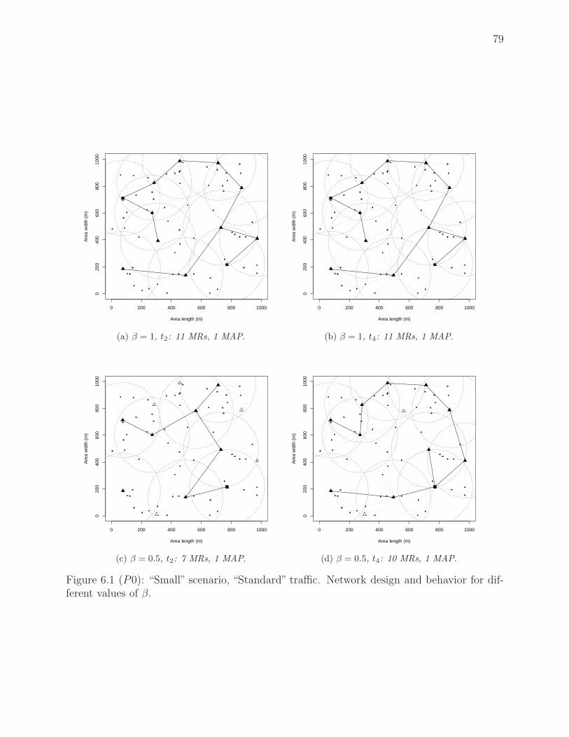
79

Area length (m)

Are

a w

idth

(m

)

0 200 400 600 800 1000

020

040

060

080

010

00

(a) β = 1, t2: 11 MRs, 1 MAP.

Area length (m)

Are

a w

idth

(m

)

0 200 400 600 800 10000

200

400

600

800

1000

(b) β = 1, t4: 11 MRs, 1 MAP.

Area length (m)

Are

a w

idth

(m

)

0 200 400 600 800 1000

020

040

060

080

010

00

(c) β = 0.5, t2: 7 MRs, 1 MAP.

Area length (m)

Are

a w

idth

(m

)

0 200 400 600 800 1000

020

040

060

080

010

00

(d) β = 0.5, t4: 10 MRs, 1 MAP.

Figure 6.1 (P0): “Small” scenario, “Standard” traffic. Network design and behavior for dif-ferent values of β.

80

Area length (m)

Are

a w

idth

(m

)

0 200 400 600 800 1000

020

040

060

080

010

00

(a) β = 1, t2: 11 MRs, 1 MAP.

Area length (m)

Are

a w

idth

(m

)

0 200 400 600 800 10000

200

400

600

800

1000

(b) β = 1, t4: 11 MRs, 1 MAP.

Area length (m)

Are

a w

idth

(m

)

0 200 400 600 800 1000

020

040

060

080

010

00

(c) β = 0.5, t2: 6 MRs, 2 MAP.

Area length (m)

Are

a w

idth

(m

)

0 200 400 600 800 1000

020

040

060

080

010

00

(d) β = 0.5, t4: 9 MRs, 2 MAP.

Figure 6.2 (P0): “Small” scenario, “Standard” traffic, variable backbone links capacity. Net-work design and behavior for different values of β.

81

Comparison with the two-step procedure

An important point that we wanted to evaluate is what is the level of savings provided by

the joint optimization when compared with the optimal energy operation of a well designed

network. To be fair, we optimized first the planning by using (P0) with β = 1, and next

we introduced the resulting network into an optimal operation model, such as the one given

in Capone et al. (2012b). The results are provided in the tables in the column titled “two-

step”. Note that in this case, since the two optimization problems are independent, it is

not possible to adjust the importance of the energy issue with respect to the installation cost

according to particular network needs. Such a regulation can be done exclusively by applying

the joint design and management approach, where the network planning and management

are handled at the same time and tuned by a proper weight parameter.

Observing first the numbers obtained for β = 1 and then the ones corresponding to lower

values of β, it is clear that by enabling the power management mechanism good energy saving

can be achieved. In particular, our joint approach produces savings that are not limited to

the minimum cost topology, but it trades off between the two terms of the objective function

to reach the best compromise of energy saving and installation cost reduction. For example,

if β = 0.5 we more than double the energy savings given by the two-step approach at the

cost of a modest increase (+4.17%) in CapEx expenses. Similarly, by investing the 29.17%

more in the installation phase, energy savings of almost 24% are possible for β = 0.1.

It must be noticed that, despite the fact that CapEx increases could seem higher than

energy savings, the latter spread during the whole period of operation, while network opera-

tors meet capital investments only once. Taking the case of β = 0.5 as an example, one can

estimate that the additional initial investments, corresponding to 400 ¤, can be recovered

from the energy saving in less than two years of network operation (259.15 ¤/year spared),

which is a short period compared to the average network life.

Cellular comparison

In Table 6.5 the same“large” scenario is considered, but in this case the MAPs only approach

is applied. Such an approach “mimics” the case of a purely cellular network. Thus, the idea

of this comparison is to determine the levels of energy savings provided by the flexibility of

mesh networks. Back to Table 6.5, we present in bold the percentage increases in CapEx

and energy expenditures with respect to the values in Table 6.4. Clearly, since only the

most expensive and energy hungry devices can be deployed and that there is no flexibility

related to mesh networking, both capital investments and power expenditures face a sensible

82

Table 6.5 Size “large”, Traffic “standard”, MAPs only approach. Summary of the results withdifferent values of β.

β = 1 β = 0.5 β = 0.1

CapEx (¤) 18000 18800 21600Capex Diff. - vs (P0) +87.50% +88.00% +74.19%

Energy (Wh/day) 19440 15876 (-18.33%) 15120 (-22.22%)Energy Diff - vs (P0) +16.38% +20.00% +17.73%

OpEx (¤/day, 0.2 ¤/kWh) 3.89 3.18 3.02Installed MAPs 45 47 54

Turned On MAPs t1 - 45 t1 - 34 t1 - 33t2 - 45 t2 - 33 t2 - 31t3 - 45 t3 - 36 t3 - 35t4 - 45 t4 - 44 t4 - 44t5 - 45 t5 - 37 t5 - 34t6 - 45 t6 - 41 t6 - 39t7 - 45 t7 - 34 t7 - 32t8 - 45 t8 - 35 t8 - 32

increase. Despite that, our joint approach applied to the cellular case still insures energy

savings of 18% for β = 0.5 with 4.44% extra CapEx and more than 22% for β = 0.1.

6.7.2 Savings obtained using the partial covering-relaxed model

Tables 6.6 and 6.7 show the results computed for the smallest scenario with respectively

standard and busy traffic profile for the partial covering-relaxed problem (P1). The Tables

show capital expenditures, the amount of energy and its cost in a day and the number of

installed gateways and routers. Moreover, energy decrease percentages obtained by compar-

ing the results with the ones of (P0) for the same scenario are reported. The column “relax

two-step” refers to the last model variation described in Section 6.6.3 which, starting from a

given complete coverage topology, manages the network so as to provide services only to the

active users. In this case, the energy decrease percentage is related to the value of energy

found by the two-step approach rather than the one of (P0). Also, in order to illustrate

the behavior of the energy management mechanism we also report the number of MRs and

MAPs switched on in every time interval.

As already noticed, by jointly optimizing installation and operation costs we can obtain

high energy savings. Significant is the case of β = 0.5: if one more MR is installed at the

modest extra cost of 200 ¤, power consumption will be reduced by almost 22%. Formulation

(P1) shows the same behavior of (P0) but, compared to the latter, (P1) can reduce the

energy expenditures of a percentage in the 9% to 15% range. This appears straightforward,

since the network service must be guaranteed only for the users providing traffic, while BSs

83

Table 6.6 Size “small”, Traffic “standard”. Summary of the results from (P1) with differentvalues of β and comparison with relaxed two-step approach.

β = 1 relax two-step β = 0.5 β = 0.1CapEx (¤) 2600 2600 2800 3400

Energy (Wh/day) 3762 3267 (-15.18%) 2952 (-21.53%) 2727 (-27.51%)OpEx (¤/day, 0.2 ¤/kWh) 0.75 0.65 0.59 0.55

Energy Diff. - vs (P0) -14.34% -6.44% (vs 2-step) -7.08% -12.93%Installed MRs - MAPs 11 - 1 11 - 1 12 - 1 11 - 3


Table 6.7 Size “small”, Traffic “busy”. Summary of the results from (P1) with different valuesof β and comparison with relaxed two-step approach.

β = 1 relax two-step β = 0.5 β = 0.1CapEx (¤) 3400 3400 3400 3600

Energy (Wh/day) 4572 3717 (-18.70%) 3672 (-19.69%) 3654 (-20.087%)OpEx (¤/day, 0.2 ¤/KWh) 0.91 0.74 0.73 0.73

Energy Diff. - vs (P0) -21.60% -9.83% (vs 2-step) -10.92% -10.38%Installed MRs - MAPs 15 - 1 15 - 1 15 - 1 14 - 2


84

covering only idle users can be powered off. Looking now at the last part of the table,

one can notice how the network devices are managed in order to minimize the total power

consumption. During lower-traffic periods (intervals 1 and 2), 9 or 5 MRs over 11 are turned

on when β = 1: the management mechanism is not able to power off other BSs due to the

small covering ray of wireless mesh devices. On the other hand, the highest number or routers

is used when the traffic presents its peak. Decreasing the value of β and focusing in particular

on β = 0.1, we observe a smaller number of active BSs in all time intervals (even 0 routers

in period 2), while a higher number of MAPs is installed and turned on in order to better

manage the traffic of the MCs. The results described above are represented in Figure 6.3.

On the left side, the solutions obtained for β = 1, 0.5 and 0.1 in time period 2 are displayed,

while solutions for time period 4 are on the right side.

For the sake of completeness, we report in Table 6.7 the results we found for the “small”

scenario where active users provide an amount of traffic between 8 and 10Mbps, what we

call the “busy” scenario. Compared to the ones in Table 6.6, the power savings are lower

as was expected given that we get less flexibility when there is more demand. Nevertheless

the approach still manages to get percentage of savings around 20% for both β = 0.5 and

β = 0.1.

Finally, in Figure 6.4 we summarize the percentage variations of capital and energy ex-

penses obtained by applying (P0) (Figure 6.4a) and (P1) (Figure 6.4b) to the three“standard”

traffic test scenarios. Each point in the graphs corresponds to the percentage increment of

CapEx and decrement of energy costs, with respect to the case of β = 1, obtained by playing

with the weight parameter.

6.8 Conclusion

In this paper we have tackled the problem of designing energy-aware wireless mesh networks.

Starting from the key idea that a wise network management is probably the best way to save

power and reduce operational expenses, we have developed an optimization framework that

selects the devices to be installed and jointly considers their dynamic energy-aware operation.

Therefore, the objective of this optimization approach is that of minimizing at the same time

capital and operational expenses, which are mostly due to energy consumption.

By mean of three test scenarios and several additional model variations, we have shown

that an optimal network topology from the installation cost point of view does not produce

a network that is optimal for an energy-aware operation and that it is necessary to plan

ahead with the use of the joint planning and operational tool. In particular, varying the

trade-off parameter β between CapEx and OpEx, we have found that important energy

85

Area length (m)

Are

a w

idth

(m

)

0 200 400 600 800 1000

020

040

060

080

010

00

(a) β = 1, t2: 5 MRs, 1 MAP.

Area length (m)

Are

a w

idth

(m

)

0 200 400 600 800 1000

020

040

060

080

010

00

(b) β = 1, t4: 11 MRs, 1 MAP.

Area length (m)

Are

a w

idth

(m

)

0 200 400 600 800 1000

020

040

060

080

010

00

(c) β = 0.5, t2: 4 MRs, 1 MAP.

Area length (m)

Are

a w

idth

(m

)

0 200 400 600 800 1000

020

040

060

080

010

00

(d) β = 0.5, t4: 10 MRs, 1 MAP.

Area length (m)

Are

a w

idth

(m

)

0 200 400 600 800 1000

020

040

060

080

010

00

(e) β = 0.1, t2: 0 MRs, 3 MAPs.

Area length (m)

Are

a w

idth

(m

)

0 200 400 600 800 1000

020

040

060

080

010

00

(f) β = 0.1, t4: 8 MRs, 3 MAPs.

Figure 6.3 (P1), “Small” scenario, “Standard” traffic. Network design and behavior for dif-ferent values of β.

86

Capex variation (%)

Ene

rgy

cost

var

iatio

n (%

)

0 10 20 30 40 50 60 70 80 90

−35

−30

−25

−20

−15

−10

−5

0 Scenario ’small’Scenario ’medium’Scenario ’large’

(a) (P0), “standard” traffic.

Capex variation (%)

Ene

rgy

cost

var

iatio

n (%

)

0 10 20 30 40 50 60 70 80 90

−35

−30

−25

−20

−15

−10

−5

0 Scenario ’small’Scenario ’medium’Scenario ’large’

(b) (P1), “standard” traffic.

Figure 6.4 Capital and energy expenses variations for different values of β.

87

savings can be reached at the cost of little increases in installation investments. Moreover,

the effectiveness of our framework has been confirmed by comparing our results with the ones

obtained from a more “traditional” two-step approach, where network planning and energy-

aware operation are optimized separately. The joint framework was also applied to a cellular

architecture, showing that it still produces good energy savings results but that they are less

important than those obtained with mesh networking. Finally, we evaluated the effect of

partial covering in the procedure and found that more than ten percent energy savings can

still be achieved when some coverage constraints are relaxed, regardless of the case, which

shows the importance of a more flexible wireless network coverage control for energy savings.

88

CHAPTER 7

ADDITIONAL MODEL VARIATIONS

7.1 Introduction

In addition to the journal papers constituting Chapters 4, 5 and 6, other articles have been

produced and presented in international conferences throughout the doctoral research. Paper

Boiardi et al. (2012c), accepted at the 21st International Conference on Computer Commu-

nications and Networks (ICCCN), summarizes the same concepts that have been extensively

explained in Chapter 5, providing preliminary results for the joint planning and energy man-

agement problem for cellular networks (JPEM-CN) LTE technology. Illustrating the early

stages of the JPEM framework applied to cellular networks, the paper does not include

supplementary original contents. However, an unpublished variation of the framework for

cellular networks have been developed, which simplify the JPEM-CN objective function by

introducing a new set of constraints to limit the CapEx. Similarly, a modified version of the

joint planning and energy management problem for wireless mesh networks (JPEM-WMN)

described in Chapter 6 is shown in Boiardi et al. (2012a), included in the proceeding of the

10th IEEE global communications conference (Globecom). Here, in order to control the en-

ergy consumed in the wake-up process, a set of constraints is introduced to limit the number

of time an access device (MR or MAP) can change its state from active to idle and vice versa.

In what follows, the JPEM-CN with CapEx budget is presented (Section 7.2); then, the

JPEM-WMN with on/off switching constraints as reported in Boiardi et al. (2012a) is illus-

trated (Section 7.3).

7.2 JPEM-CN with CapEx budget constraints

As already pointed out, the joint planning and energy management model for cellular net-

works introduced in Section 5.6 is computationally very complex. As a matter of fact, the

numerical tests presented in Chapter 5 were obtained by setting the optimality gap at 5%

for most of the instances, so as to bound the resolution time to 30 minutes or less. However,

the massive increase in complexity when larger instances are considered makes it impossible

to examine any real size scenario.

A variation of the JPEM-CN problem has been developed to reduce the complexity of the

mathematical model and to improve the consistency of the original formulation, a variation of

the JPEM-CN problem has been developed where the CapEx term is removed from objective

89

function (5.7), leaving

ϕ∑

j∈S

∑

k∈Kj

∑

t∈T

ǫjkδtyjkt+ϑ∑

i∈It

∑

j∈S

∑

t∈T

xijtδtrij (7.1)

As reported in Section 5.6, parameters ǫjk represent the power consumed by a BS located

in site j with configuration k, parameters δt measure the duration of time period t while

parameters rij correspond to the distance between TP i and a BS in j. Decision variables

yjkt and xijt equal 1 if, respectively, a BS in site j with configuration k is active in time t

and if Traffic TP i is assigned to a BS located in j during time t. Parameter ϕ, defined as in

Section 5.6, symbolizes the cost of the energy consumption over the network lifetime. Since

only the OpEx component is minimized in the new objective function (7.1), β is no longer

needed to trade-off between the capital and energy costs; on the other hand, parameter ϑ is

used to weigh the importance of the third part of the objective function, which guarantees

the quality of the connection between test points and base stations.

The new formulation requires the introduction of an additional parameter B, defining the

available capital budget for the installation of the access devices. In order to impose a limit

on the maximum CapEx allowed in the network deployment phase, a budget constraint is

also added to the model:

∑

j∈S

∑

k∈Kj

zjkγjk ≤ B (7.2)

Parameters γjk represent the cost of installing a BS with configuration k in site j, while

variables zjk are set to 1 if a BS is installed in site j with configuration k. Thus, the

JPEM-CN with budget constraints, which will be called Budget JPEM-CN, is defined as

follows:

90

min (7.1) OpEx

ϕ∑

j∈S

∑

k∈Kj

∑

t∈T

ǫjkδtyjkt+ϑ∑

i∈It

∑

j∈S

∑

t∈T

xijtδtrij

subject to: (7.2) CapEx budget constraints∑

j∈S

∑

k∈Kj

zjkγjk ≤ B

(5.8) Coverage constraints∑

j∈S

∑

k∈Kj

aijkyjkt ≥ 1 ∀i ∈ Ic ∪ It, t ∈ T

(5.9) Traffic TP coverage constraints

xijt ≤∑

k∈Kj

aijkyjkt ∀i ∈ It, j ∈ S, t ∈ T

(5.10) BS capacity constraints∑

i∈It

xijtpit ≤∑

k∈Kj

cjkyjkt ∀j ∈ S, t ∈ T

(5.11) Traffic TP assignment constraints∑

j∈S

xijt = 1 ∀i ∈ It, t ∈ T

(5.12) Variable y and z linking constraints

yjkt ≤ zjk ∀j ∈ S, k ∈ Kj, t ∈ T

(5.13) Single configuration constraints∑

k∈Kj

zjk ≤ 1 ∀j ∈ S

(5.14)− (5.16) Domain of decision variables

zjk, xijt, yjkt ∈ {0, 1} ∀j ∈ S, k ∈ Kj,∈ It, t ∈ T

Additional parameters used in this formulation and introduced in Section 5.6 include aijk,

equal to 1 if TP i is in the coverage area of a BS placed in site j with configuration k, pit,

measuring the traffic provided by Traffic TP i in time period t, and cjk, which represent the

capacity of a BS installed in j with configuration k.

91

7.2.1 Model variations and numerical results

The Budget JPEM-CN has been tested by considering the same scenarios used on the original

framework and displayed in Table 5.2:

- “Scenario 1”, with 40 candidate sites (CSs), 121 coverage test points (CTPs) and 30

traffic test points (TTPs) on a square area of 2000 m × 2000 m;

- “Scenario 2”, with 60 CSs, 676 Coverage TPs and 60 Traffic TPs on a square area of

5000 m × 5000 m;

- “Scenario 3”, with 120 CSs, 441 Coverage TPs and 40 Traffic TPs on a square area of

4000 m × 4000 m;

- “Scenario 3a-b-c”, a set of test instances having the same characteristics of Scenario 3,

but allowing only two BS configurations to be installed in the area (Scenario 3a: C1

and C2, Scenario 3b: C1 and C3, Scenario 3c: C2 and C3).

The value of the CapEx budget B varies according to the dimensions of the studied scenario.

Define B as the CapEx of the minimum cost topology, that is, the CapEx resulting from the

original JPEM-CN applied to the same scenario with β = 0. Considering B as the initial

amount for each test instance, values of budget have been tested being 10%, 20% and 30%

higher. To obtain the numerical examples reported below, the trade-off parameter ϑ was

set to 0.01. Even though the same parameter equals zero in the examples shown in Section

5.7.3, a fair comparison can be carried on between the JPEM-CN framework and its Budget

variation; in fact, in case of LTE test instances the objective function component insuring a

better connection quality between users and access devices does not have any impact on the

problem resolution (see Section 5.6). Finally, once again the optimality gap was set at 5%

so as to evaluate the benefits (if any) of the Budget formulation with respect to the original

joint framework.

For the sake of completeness, a partial coverage version of the Budget JPEM-CN was

also developed. As explained in Section 5.7.2 for the original formulation, here the network

service is provided only to those TTPs that are requiring traffic during a certain time period,

so that BSs covering only inactive users can be switched off. Parameter mit is introduced

to realize the limited coverage of the area, which is equal to 1 if Traffic TP i is active in

time interval t. Similarly to the case of the original JPEM-CN, coverage constraints (5.8)

and Traffic TP assignment constraints (5.11) are replaced by constraints (5.17) and (5.18),

which guarantee that every TP is in the covering radius of at least one installed BS but only

active ones are provided with network service by tuned-on access devices. Thus, the partial

coverage Budget JPEM-CN can be written as:

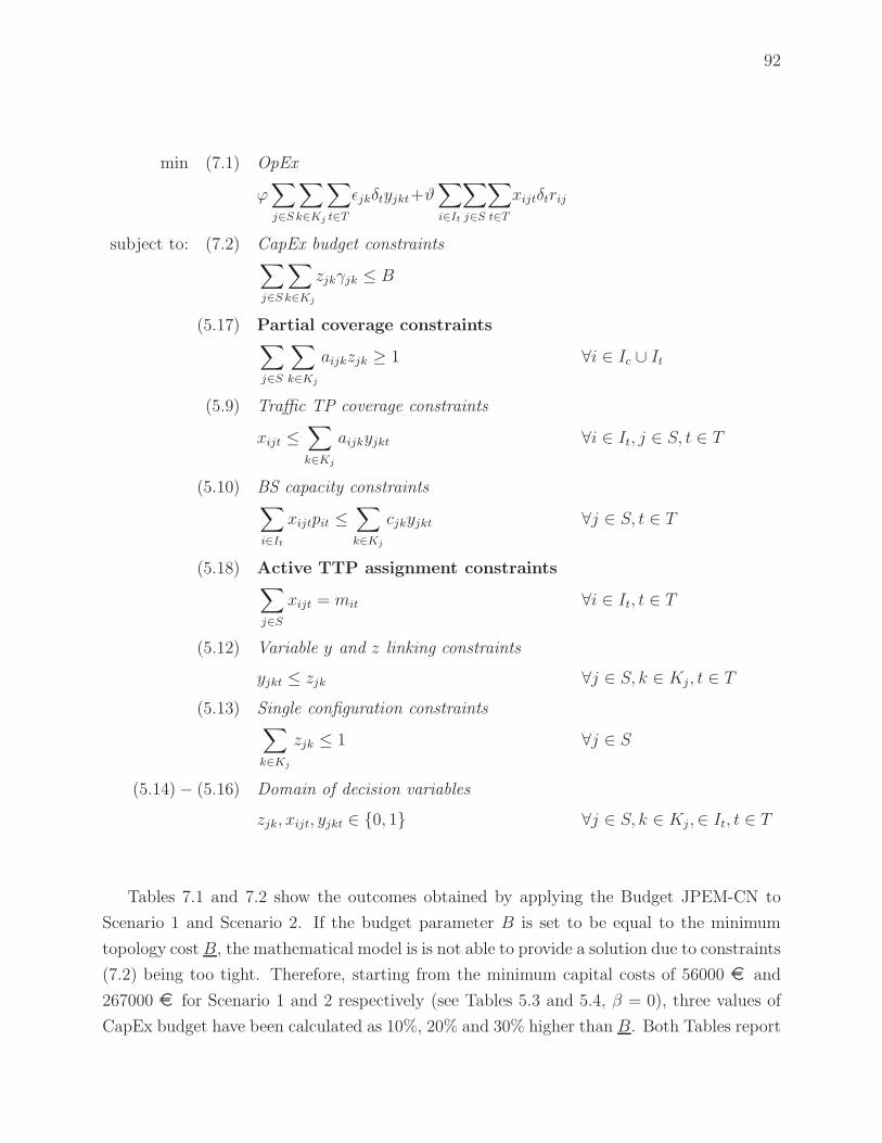
92

min (7.1) OpEx

ϕ∑

j∈S

∑

k∈Kj

∑

t∈T

ǫjkδtyjkt+ϑ∑

i∈It

∑

j∈S

∑

t∈T

xijtδtrij

subject to: (7.2) CapEx budget constraints∑

j∈S

∑

k∈Kj

zjkγjk ≤ B

(5.17) Partial coverage constraints∑

j∈S

∑

k∈Kj

aijkzjk ≥ 1 ∀i ∈ Ic ∪ It

(5.9) Traffic TP coverage constraints

xijt ≤∑

k∈Kj

aijkyjkt ∀i ∈ It, j ∈ S, t ∈ T

(5.10) BS capacity constraints∑

i∈It

xijtpit ≤∑

k∈Kj

cjkyjkt ∀j ∈ S, t ∈ T

(5.18) Active TTP assignment constraints∑

j∈S

xijt = mit ∀i ∈ It, t ∈ T

(5.12) Variable y and z linking constraints

yjkt ≤ zjk ∀j ∈ S, k ∈ Kj, t ∈ T

(5.13) Single configuration constraints∑

k∈Kj

zjk ≤ 1 ∀j ∈ S

(5.14)− (5.16) Domain of decision variables

zjk, xijt, yjkt ∈ {0, 1} ∀j ∈ S, k ∈ Kj,∈ It, t ∈ T

Tables 7.1 and 7.2 show the outcomes obtained by applying the Budget JPEM-CN to

Scenario 1 and Scenario 2. If the budget parameter B is set to be equal to the minimum

topology cost B, the mathematical model is is not able to provide a solution due to constraints

(7.2) being too tight. Therefore, starting from the minimum capital costs of 56000 ¤ and

267000 ¤ for Scenario 1 and 2 respectively (see Tables 5.3 and 5.4, β = 0), three values of

CapEx budget have been calculated as 10%, 20% and 30% higher than B. Both Tables report

93

Table 7.1 Summary of the results obtained from the Budget JPEM-CN with total coverage,Scenario 1.

B = 61.6 k B = 67.2 k B = 72.8 kB + 10% B + 20% B + 30%

Time 1 h 15 min 55 sec 1 min 16 sec 6 min 5 secCapEx (k¤) 58 56 (-3%) 68 (+17%)

Vs. JPEM-CN, β = 0 +4% +0% +21%OpEx (k¤, 8 y, 0.35¤/kWh) 40 18 (-55%) 18 (-55%)

Vs. JPEM-CN, β = 0 -5% -57% -57%Installed BSs 20 22 23

Configuration Types C1 - 1 C1 - 0 C1 - 0C2 - 1 C2 - 5 C2 - 5C3 - 18 C3 - 17 C3 - 18

Turned On BSs t1 - 16 t1 - 17 t1 - 18t2 - 9 t2 - 10 t2 - 10t3 - 7 t3 - 4 t3 - 4t4 - 9 t4 - 10 t4 - 10t5 - 14 t5 - 15 t5 - 16t6 - 14 t6 - 15 t6 - 15t7 - 15 t7 - 18 t7 - 17t8 - 17 t8 - 18 t8 - 18

Table 7.2 Summary of the results obtained from the Budget JPEM-CN with total coverage,Scenario 2.

B = 293.7 k B = 320.4 k B = 347.1 kB + 10% B + 20% B + 30%

Time 2 min 15 sec 1 min 12 sec 1 min 54 secCapEx (k¤) 292 318 (+9%) 341 (+17%)

Vs. JPEM-CN, β = 0 +9% +19% +28%OpEx (k¤, 8 y, 0.35¤/kWh) 115 117 (+2%) 114 (-0.8%)

Vs. JPEM-CN, β = 0 -43% -42% -44%Installed BSs 36 35 38



94

the problem solving time, the capital investments related to the deployed network topology,

the operational costs during an eight-year period, the number and type of installed BS as

well as the amount of access stations switched on. Percentages in parenthesis refer to the

results in column B+10%, while percentages in bold report the CapEx and OpEx difference

with respect to the results of the original JPEM-CN tested on the same scenario with β = 0,

i.e., minimum cost, unmanaged topology.

The first observation concerns the computational time required by the tested examples.

Differently from what expected, the Budget model shows an inconsistent behavior: while for

the majority of the instances a solution is reached in a few minutes, in one case the problem

is solved in more than one hour (Table 7.1, B=B+10%). The reason could be the proximity

of B to the minimum CapEx value B. Consider now Tables 7.3 and 7.4, where results for

the Budget JPEM-CN with partial area coverage are displayed. Observing in particular the

results for Scenario 1 in Table 7.3, it can be noticed that not only the B+10%, but also the

B+30% instance is highly time consuming. Therefore, budget constraints (7.2) and the value

of B seem not to be directly responsible for the Budget framework complexity.

Focusing on the percentages of energy savings achievable with growing values of B, Tables

7.1 and 7.2 clearly underline how, over a certain threshold, the model does not provide

any further improvements in power consumption reduction. Take for instance Table 7.1,

where the results related to Scenario 1 are reported in case of complete network coverage.

The big “leap” in energy savings happens for B=B+20%, when as much as 57% OpEx

cutback is reached with respect to the unmanaged minimum cost topology (see Table 5.3)

without any extra capital investment. On the other hand, B=B+10% only brings a total 5%

power reduction while B=B+30% entails a 21% higher CapEx but guarantees no additional

decreases in energy expenses. In this case, it is also interesting to compare the devices

deployed in the minimum cost topology without network management (1 C1, 1 C2 and

16 C3 BSs) to the access stations installed in correspondence of the decisive power savings

increase for B=B+10% (0 C1, 5 C2 and 17 C3 BSs). As observed for the original JPEM-CN,

even maintaining the same value of capital costs, a higher number of small cells replacing

bigger ones provides more network flexibility and thus, more opportunities for energy savings.

Similar considerations apply to Scenario 2 in Table 7.2, where a great decrease in energy

consumption is register for B=B+10%, while a less pronounced but similar behavior can be

identified in Tables 7.3 and 7.4.

Finally, Table 7.5 shows the results from Scenario 3 and its variations by applying the

total (first section) and the partial area coverage (second section) Budget JPEM-CN with

B =B+10% is reported. These results can be compared with the ones displayed in Table

5.7, where the same scenarios are solved by means of the complete and partial coverage

95

Table 7.3 Summary of the results obtained from the Budget JPEM-CN with partial coverage,Scenario 1.

B = 61.6 k B = 67.2 k B = 72.8 kB+10% B+20% B+30%

Time 2 h 17 min 15 min 1 sec 1 h 25 min 53 minCapEx (k¤) 58 67 (+16%) 68 (+17%)

Vs. JPEM-CN Partial Coverage, β = 0 +4% +20% +21%OpEx (k¤, 8 y, 0.35¤/kWh) 32 14 (-56%) 14 (-56%)

Vs. JPEM-CN Partial Coverage, β = 0 -24% -67% -67%Installed BSs 20 22 22



Table 7.4 Summary of the results obtained from the Budget JPEM-CN with partial coverage,Scenario 2.

B = 293.7 k B = 320.4 k B = 347.1 kB + 10% B + 20% B + 30%

Time 1 min 48 sec 8 min 48 sec 6 min 31 secCapEx (k¤) 293 320 (+9%) 342 (+17%)

Vs. JPEM-CN Partial Coverage, β = 0 +10% +20% +28%OpEx (k¤, 8 y, 0.35¤/kWh) 87 80 (-8%) 74 (-15%)

Vs. JPEM-CN Partial Coverage, β = 0 -57% -61% -64%Installed BSs 35 35 39



96

Table 7.5 Important results obtained from the Budget JPEM-CN with total and partialcoverage (B = B+10%), Scenario 3 and its variations.


Budget (k¤) 150.7 231 210.1 150.7CapEx (k¤) 150 - 202 (+35%) 141 (-6%)

OpEx (k¤, 8 y, 0.35¤/kWh) 47 - 198 (+321%) 46 (-2%)Installed BSs C1 - 0 C1 - - C1 - 6 C1 - n.a.

C2 - 13 C2 - - C2 - n.a. C2 - 12C3 - 34 C3 - n.a. C3 - 22 C3 - 21

Turned On BSs in t3 C1 - 0 C1 - - C1 - 6 C1 - n.a.C2 - 13 C2 - - C2 - n.a. C2 - 12C3 - 5 C3 - n.a. C3 - 5 C3 - 7


Partial Coverage:Budget (k¤) 150.7 231 210.1 150.7CapEx (k¤) 150 - 210 (+40%) 150 (-0%)

OpEx (k¤, 8 y, 0.35¤/kWh) 11 - 53 (+381%) 11 (-0%)Installed BSs C1 - 0 C1 - - C1 - 6 C1 - n.a.

C2 - 12 C2 - - C2 - n.a. C2 - 12C3 - 30 C3 - n.a. C3 - 30 C3 - 30



97

versions of the original JPEM-CN. In all cases, the original and Budget frameworks reach

very close outcomes; however, predictably, when only large cells are allowed to be installed in

the considered area (Scenario 3a), the Budget variation fails in providing a feasible solution

that satisfies at the same time the traffic coverage and the budget constraints.

From the presented results it is possible to conclude that, when a budget constraint is im-

posed by the network operator on the capital investments, the framework proposed in Section

7.2.1 represents an effective and reliable formulation for the deployment and management of

cellular networks.

7.3 JPEM-WMN with on/off switching constraints

The JPEM-WMN framework as originally formulated (see Section 6.5.2) allows the access

devices, namely mesh routers (MRs) and mesh access points (MAPs), to be turned on and

put to sleep as many times as necessary to reach the best trade-off between CapEx and

OpEx. Although the costs of a device activation from the idle state have not been considered

in the problem formulation, continuous changes in the state of MRs and MAPs can influence

negatively the energy bill as well as compromise the correct device functioning.

To cope with this issue, an interesting variation of the JPEM-WMN model was developed

and presented in Boiardi et al. (2012a), where a maximum limitation is introduced on the

number of times each installed BS can change its state from on to off and vice versa. Two

sets of auxiliary variables were added to the original formulation:

vjt =

1 if a MR installed in site j ∈ S change its state

from time t− 1 to time t ∈ T ,

0 otherwise.

(7.3)

gjt =

1 if a MAP installed in site j ∈ S change its state

from time t− 1 to time t ∈ T ,

0 otherwise.

(7.4)

The new auxiliary constraints (7.5) to (7.8), replacing respectively the non linear expressions

vjt ≥ |yjt − yjt−1| and gjt ≥ |rjt − rjt−1|, help counting the number of state changes for each

98

access device:

vjt ≥ yjt − yjt−1 ∀j ∈ S, t ∈ T/{t1} (7.5)

vjt ≥ yjt−1 − yjt ∀j ∈ S, t ∈ T/{t1} (7.6)

gjt ≥ rjt − rjt−1 ∀j ∈ S, t ∈ T/{t1} (7.7)

gjt ≥ rjt−1 − rjt ∀j ∈ S, t ∈ T/{t1} (7.8)

State change constraints (7.9) and (7.10) limit the number of state switches to a chosen value

η1 for routers and η2 for access points.

∑

t∈T/{t1}

vjt ≤ η1 ∀j ∈ S (7.9)

∑

t∈T/{t1}

gjt ≤ η2 ∀j ∈ S (7.10)

Finally, domain constraints have to be added for the auxiliary variables:

vjt ∈ {0, 1} ∀j ∈ S, t ∈ T/{t1} (7.11)

gjt ∈ {0, 1} ∀j ∈ S, t ∈ T/{t1} (7.12)

The JPEM-WMN with on/off switching constraints, from now on denominated On/Off

JPEM-WMN, is defined as:

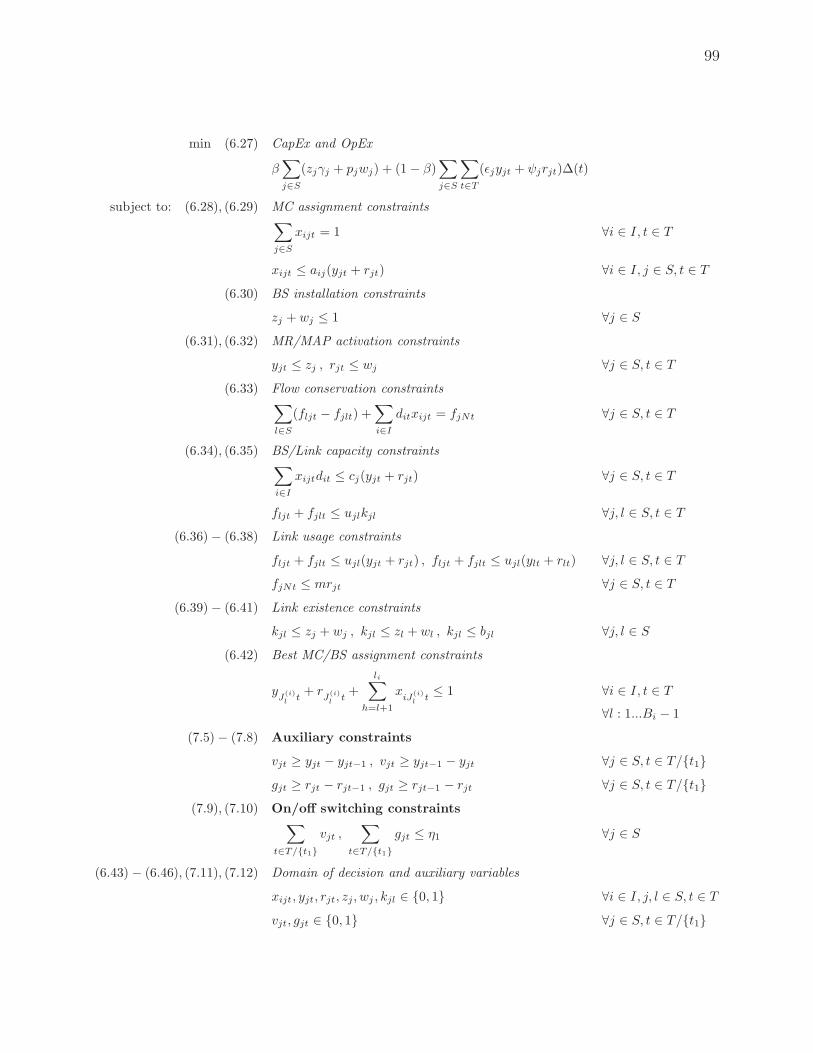
99

min (6.27) CapEx and OpEx

β∑

j∈S

(zjγj + pjwj) + (1− β)∑

j∈S

∑

t∈T

(ǫjyjt + ψjrjt)∆(t)

subject to: (6.28), (6.29) MC assignment constraints∑

j∈S

xijt = 1 ∀i ∈ I, t ∈ T

xijt ≤ aij(yjt + rjt) ∀i ∈ I, j ∈ S, t ∈ T

(6.30) BS installation constraints

zj + wj ≤ 1 ∀j ∈ S

(6.31), (6.32) MR/MAP activation constraints

yjt ≤ zj , rjt ≤ wj ∀j ∈ S, t ∈ T

(6.33) Flow conservation constraints∑

l∈S


i∈I

ditxijt = fjNt ∀j ∈ S, t ∈ T

(6.34), (6.35) BS/Link capacity constraints∑

i∈I

xijtdit ≤ cj(yjt + rjt) ∀j ∈ S, t ∈ T

fljt + fjlt ≤ ujlkjl ∀j, l ∈ S, t ∈ T

(6.36)− (6.38) Link usage constraints

fljt + fjlt ≤ ujl(yjt + rjt) , fljt + fjlt ≤ ujl(ylt + rlt) ∀j, l ∈ S, t ∈ T

fjNt ≤ mrjt ∀j ∈ S, t ∈ T

(6.39)− (6.41) Link existence constraints

kjl ≤ zj + wj , kjl ≤ zl + wl , kjl ≤ bjl ∀j, l ∈ S

(6.42) Best MC/BS assignment constraints

yJ

(i)l

t+ r

J(i)l

t+

li∑

h=l+1

xiJ

(i)l

t≤ 1 ∀i ∈ I, t ∈ T

∀l : 1...Bi − 1

(7.5)− (7.8) Auxiliary constraints

vjt ≥ yjt − yjt−1 , vjt ≥ yjt−1 − yjt ∀j ∈ S, t ∈ T/{t1}

gjt ≥ rjt − rjt−1 , gjt ≥ rjt−1 − rjt ∀j ∈ S, t ∈ T/{t1}

(7.9), (7.10) On/off switching constraints∑

t∈T/{t1}

vjt ,∑

t∈T/{t1}

gjt ≤ η1 ∀j ∈ S

(6.43)− (6.46), (7.11), (7.12) Domain of decision and auxiliary variables

xijt, yjt, rjt, zj, wj , kjl ∈ {0, 1} ∀i ∈ I, j, l ∈ S, t ∈ T

vjt, gjt ∈ {0, 1} ∀j ∈ S, t ∈ T/{t1}

100

The model parameters are defined as in Section 6.5. Parameters γj and pj represent respec-

tively the installation costs of a MR or MAP installed in site j, while their power consumption

is measured by ǫj and ψj . ∆(t) is the duration of time period t. Parameters cj, m and ujl

quantify the access capacity of a BS located in site j, the MAP’s Internet access capacity

and the capacity of the link between BSs installed in sites j and l. Parameters aij and bjl

are equal to 1 if, respectively, MC i is in the coverage area of BS j and if a link between

BSs installed in sites j and l is possible. The traffic provided by MC i in time period t is

represented by dit, while Bi counts the number of BSs covering MC i. As for the model

variables, zj and wj are equal to 1 if a MR or MAP is installed in site j, while yjt and rjt are

equal to 1 if an installed MR or MAP is active in time period t. Variables xijt express if MC

i is assigned to a BS installed in site j in time t and variables kjl equal 1 if a link between

BSs installed in j and l exists. Finally, variables fjlt and fjNt represent the flow between BSs

located in j and l and the flow between a MAP installed in j and the Internet (N) during

time t.

7.3.1 Model variations and numerical results

Numerical results were produced to compare the modified formulation described above with

the original JPEM-WMN framework. The same test scenarios reported in Table 6.2 have

been considered:

- “Small”, counting 13 candidate sites (CSs) and 60 mesh clients (MCs) on a square area

of 1000 m × 1000 m;

- “Medium”, counting 40 CSs and 130 MCs on a square area of 1500 m × 1500 m;

- “Large”, counting 64 CSs and 240 MCs on a square area of 2500 m × 2500 m.

In this case, only the standard traffic profile is taken into account, that is, each MC is

randomly assigned by the instance generator with a traffic value ranging between 1 and 10

Mb/s. Also, the limit on the number of state changes has been set to 1 for both MRs and

MAPs (η1 and η2, respectively).

As done for the original formulation described in Section 6.5.2, different problem variations

were tested:

• The two-step approach, which divides the On/Off JPEM-WMN in two separate

phases. First, the minimum cost network topology is obtained by running the model

proposed above by setting β to 1, that is, by dropping the OpEx term from the objective

function; then, the management of the deployed devices is optimized by means of the

framework proposed in Capone et al. (2012b).

101

• The on/off switching constraints relaxation, representing the original JPEM-WMN

problem, where no limit is imposed on the number of state changes of the access devices;

• The cellular comparison, where only mesh access points (MAPs) can be installed in

the area. Here, the multi-hop behavior typical of WMNs is replaced by a topology where

every access device is directly connected to the backbone and thus, to the Internet.

• The partial covering-relaxed problem, where the network service is provided only

to active customers in every time instance. Installed access points that cover only idle

customers can be turned off. In this case, as reported in Section 6.5.3 for the original

framework, an additional binary parameters hit have to be introduced, which is equal to

1 is MC i is providing traffic in time period t. Once again, MC assignment constraints

(6.29) have to be replaced by constraints (6.47), responsible for limiting the network

coverage only to active MCs.

Table 7.6 compares the energy saving percentages obtained from the On/Off JPEM-WMN

and the ones resulting from the original version of the framework. Each percentage entry,

identifying the savings achieved in correspondence of a certain value of the trade-off param-

eter β, refers to the energy requirements of the same test scenario when β = 1. In that case,

the operational expenses are ignored and the model simply provides a network design opti-

mization according to the minimum installation costs criterion. The percentages reported in

parenthesis show the additional savings that can be reached if the state switching constraints

are relaxed, i.e., if the access stations are free to change their activity state. Important en-

ergy savings can be obtained when installation and management are jointly optimized. As

expected, the relaxation of the on/off switching constraints allows even lower power expen-

ditures; the deployed network is more flexible, and only the access devices that are necessary

to route the traffic or cover the MCs are maintained on.

A better insight on the effect of the on/off constraints relaxation on the network topology is

provided in Table 7.7, where the results obtained by exploiting the two-step approach are also

Table 7.6 Energy saving percentages obtained from the JPEM-WMN with or without theon/off switching constraints in all test scenarios (percentages are referred to the cases ofβ = 1).

Small Medium Large

β = 0.8 15.37% 7.75% 12.12%On/off JPEM-WMN β = 0.5 20.50% 10.33% 12.40%

β = 0.1 23.77% 14.67% 15.46%

β = 0.8 20.49% (+6.05% ) 12.39% (+5.04% ) 27.66% (+6.62% )JPEM-WMN β = 0.5 27.66% (+9.17% ) 14.98% (+5.18% ) 20.87% (+9.59% )

β = 0.1 27.66% (+5.10% ) 20.80% (+7.26% ) 23.11% (+9.05% )

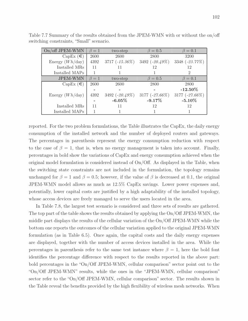
102

Table 7.7 Summary of the results obtained from the JPEM-WMN with or without the on/offswitching constraints, “Small” scenario.

On/off JPEM-WMN β = 1 two-step β = 0.5 β = 0.1

CapEx (¤) 2600 2600 2800 3200Energy (Wh/day) 4392 3717 (-15.36% ) 3492 (-20.49% ) 3348 (-23.77% )


JPEM-WMN β = 1 two-step β = 0.5 β = 0.1

CapEx (¤) 2600 2600 2800 2800- - - -12.50%

Energy (Wh/day) 4392 3492 (-20.49% ) 3177 (-27.66% ) 3177 (-27.66% )- -6.05% -9.17% -5.10%


reported. For the two problem formulations, the Table illustrates the CapEx, the daily energy

consumption of the installed network and the number of deployed routers and gateways.

The percentages in parenthesis represent the energy consumption reduction with respect

to the case of β = 1, that is, when no energy management is taken into account. Finally,

percentages in bold show the variations of CapEx and energy consumption achieved when the

original model formulation is considered instead of On/Off. As displayed in the Table, when

the switching state constraints are not included in the formulation, the topology remains

unchanged for β = 1 and β = 0.5; however, if the value of β is decreased at 0.1, the original

JPEM-WMN model allows as much as 12.5% CapEx savings. Lower power expenses and,

potentially, lower capital costs are justified by a high adaptability of the installed topology,

whose access devices are freely managed to serve the users located in the area.

In Table 7.8, the largest test scenario is considered and three sets of results are gathered.

The top part of the table shows the results obtained by applying the On/Off JPEM-WMN, the

middle part displays the results of the cellular variation of the On/Off JPEM-WMN while the

bottom one reports the outcomes of the cellular variation applied to the original JPEM-WMN

formulation (as in Table 6.5). Once again, the capital costs and the daily energy expenses

are displayed, together with the number of access devices installed in the area. While the

percentages in parenthesis refer to the same test instance where β = 1, here the bold font

identifies the percentage difference with respect to the results reported in the above part:

bold percentages in the “On/Off JPEM-WMN, cellular comparison” sector point out to the

“On/Off JPEM-WMN” results, while the ones in the “JPEM-WMN, cellular comparison”

sector refer to the “On/Off JPEM-WMN, cellular comparison” sector. The results shown in

the Table reveal the benefits provided by the high flexibility of wireless mesh networks. When

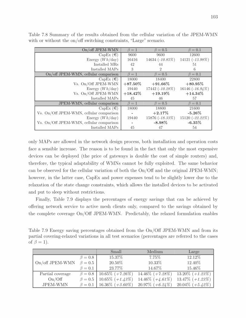
103

Table 7.8 Summary of the results obtained from the cellular variation of the JPEM-WMNwith or without the on/off switching constraints, “Large” scenario.

On/off JPEM-WMN β = 1 β = 0.5 β = 0.1CapEx (¤) 9600 9600 12600

Energy (Wh/day) 16416 14634 (-10.85% ) 14121 (-13.98% )Installed MRs 42 44 51

Installed MAPs 3 2 6On/off JPEM-WMN, cellular comparison β = 1 β = 0.5 β = 0.1

CapEx (¤) 18000 18400 22800Vs. On/Off JPEM-WMN +87.50% +91.66% +80.95%

Energy (Wh/day) 19440 17442 (-10.28% ) 16146 (-16.94% )Vs. On/Off JPEM-WMN +18.42% +19.19% +14.34%

Installed MAPs 45 46 57JPEM-WMN, cellular comparison β = 1 β = 0.5 β = 0.1

CapEx (¤) 18000 18800 21600Vs. On/Off JPEM-WMN, cellular comparison - +2.17% -5.26%

Energy (Wh/day) 19440 15876 (-18.33% ) 15120 (-22.22% )Vs. On/Off JPEM-WMN, cellular comparison - -8.98% -6.35%

Installed MAPs 45 47 54

only MAPs are allowed in the network design process, both installation and operation costs

face a sensible increase. The reason is to be found in the fact that only the most expensive

devices can be deployed (the price of gateways is double the cost of simple routers) and,

therefore, the typical adaptability of WMNs cannot be fully exploited. The same behavior

can be observed for the cellular variation of both the On/Off and the original JPEM-WMN;

however, in the latter case, CapEx and power expenses tend to be slightly lower due to the

relaxation of the state change constraints, which allows the installed devices to be activated

and put to sleep without restrictions.

Finally, Table 7.9 displays the percentages of energy savings that can be achieved by

offering network service to active mesh clients only, compared to the savings obtained by

the complete coverage On/Off JPEM-WMN. Predictably, the relaxed formulation enables

Table 7.9 Energy saving percentages obtained from the On/Off JPEM-WMN and from itspartial covering-relaxed variations in all test scenarios (percentages are referred to the casesof β = 1).

Small Medium Large

β = 0.8 15.37% 7.75% 12.12%On/off JPEM-WMN β = 0.5 20.50% 10.33% 12.40%

β = 0.1 23.77% 14.67% 15.46%

Partial coverage β = 0.8 10.65% (+7.26% ) 14.46% (+7.28% ) 13.20% (+1.23% )On/Off β = 0.5 10.65% (+1.43% ) 14.46% (+4.61% ) 13.47% (+1.23% )

JPEM-WMN β = 0.1 16.36% (+3.60% ) 20.97% (+6.24% ) 20.04% (+5.42% )

104

slightly higher power savings with respect to the reference framework due to the lower number

of customers requiring coverage; however, more striking saving values are prevented by the

effect of constraints (7.9) and (7.10), which limit to one the number of state changes allowed

to each access device. As foreseeable, removing the on/off switching constraints results in a

more efficient network management, as shown in Table 6.7 and displayed in Figure 6.3.

105

CHAPTER 8

HEURISTIC RESOLUTION

8.1 Introduction

As already pointed out, the joint planning and energy management problem for cellular

networks (JPEM-CN) is computationally very expensive. This complexity has limited the

analysis only to the small test instances presented in Section 5.7, where a maximum of 120

candidate sites and 60 traffic test points are considered in a single scenario. Moreover, the

solutions are never optimal but always obtained by stopping the optimization at 5% gap to

the lower bound (or below, in some cases).

In order to simplify the application of the joint framework and allow the investigation of

larger test examples, an heuristic method has been developed. By separating the design and

the operation management problems and addressing only specific time periods, the proposed

heuristic computes a partial topology that serves as initial solution for the original JPEM-CN.

This way, the solving time for the toy scenarios displayed in Table 5.2 is reduced while the

resolution of real-size instances is at last possible.

In this chapter, the technique is explained and illustrated (Section 8.2). It is evaluated

in Section 8.3, where the results from the toy scenarios are compared to the results obtained

from the JPEM-CN. Finally, Section 8.4 introduces new, bigger test instances and shows the

performance of the heuristic in terms of solving time.

8.2 Heuristic Method for JPEM-CN

The joint planning and energy management problem for cellular networks as described in

Section 5 is a powerful planning tool, able to find the best network deployment based on its

installation costs and its energy saving capabilities. The framework has proven its effective-

ness and benefits compared to a more traditional approach where the operation management

is performed on a pre-installed network; however, the computational complexity of the model

formulation limits its application only to small-size test instances.

The heuristic developed during the doctoral research aims at decreasing the solving time

for toy examples and allowing the resolution of test scenarios whose size is comparable with

real-life situations. The idea lying behind the proposed method is that a solution can be

reached faster if the JPEM-CN framework is provided in input with a partial topology from

which the optimization can start off. The heuristic approach develops according to the

106

Figure 8.1 Schematics of the heuristic method for JPEM-CN.

107

diagram reported in Figure 8.1. In what follows, its phases are separately presented and

described in more detail.

Preliminary - Selection of the considered time periods

The division of the day in multiple time periods, each one characterized by a different traffic

profile value, and the necessity of topological continuity between them constitute one of

the most challenging aspects of the JPEM-CN. Naturally, in order to reduce the problem

complexity and formulate a heuristic, one of the first decisions to be taken is how to deal

with the time dimension. In particular, it is fundamental to determine which time periods

should be examined and in which way they should be connected to one another.

Between the eight time intervals considered for the cellular network examples and dis-

played in Figure 5.1, two of them can be identified as particularly significant:

- The peak traffic time t8, during which the highest traffic volume has to be served by an

elevated number of access stations;

- The off-peak time t3, when the highest number of access devices can potentially be

turned off to reduce the energy expenses.

Thus, in the heuristic’s phase I, only the intervals t8 and t3 and the corresponding traffic values

are taken into account, while the remaining periods of the day are temporary neglected and

reconsidered in phase II. As it happens in the original problem formulation, a connection is

maintained between these time periods; more details on the issue are provided in the next

phases.

Phase I.I - Energy Management problem for time tr

Once the time periods of interest have been chosen, their traffic information are exploited in

succession to perform the operation management of a fictitious complete topology, where all

the base station configurations are installed in every candidate site. Such an initial topology

has been chosen to guarantee that the selected activation pattern is effectively the most

energy efficient one for the first time. In this regard, it is important to note that the order in

which the time instances are considered influences the outcome of the heuristic; therefore, the

heuristic has been tested by analyzing first the peak time t8 and then the off-peak time t3 and

vice versa. Here, to avoid any confusion, the first and second time periods to be evaluated

are identified respectively as tr and ts.

Consider now tr and the corresponding registered traffic data. Given a complete topol-

ogy, the energy management problem for cellular networks (EM-CN) is used to find the BS

activation pattern with lowest energy consumption during tr. The EM-CN can be modeled

108

by borrowing parameters, variables and constraints from the original and Budget versions of

the JPEM-CN; however, modifications are necessary to drop the time indexes and to account

for the pre-installed access devices.

min ϕ∑

j∈S

∑

k∈Kj

ǫjkδtry′jk (8.1)

subject to:∑

j∈S

∑

k∈Kj

aijky′jk ≥ 1 ∀i ∈ Ic ∪ It (8.2)

x′ij ≤∑

k∈Kj

aijky′jk ∀i ∈ It, j ∈ S (8.3)

∑

i∈It

x′ijpitr ≤∑

k∈Kj

cjky′jk ∀j ∈ S (8.4)

∑

j∈S

x′ij = 1 ∀i ∈ It (8.5)

∑

k∈Kj

y′jk ≤ 1 ∀j ∈ S (8.6)

x′ij , y′jk ∈ {0, 1} ∀j ∈ S, k ∈ Kj , i ∈ It (8.7)

As in the previous formulations, parameters ǫjk and cjk represent the energy consumption

and the capacity of a BS located in j with configuration k, δtr is the duration in hours of

time tr and pitr measures the traffic offered by Traffic TP i during time tr. Parameter ϕ

symbolizes the cost of the power consumption over the network lifetime. Since the network

topology is known, installation variables are excluded from the formulations; on the other

hand, the time index has been dropped for the activation variables y′jk, which are equal to

1 if the access station located in j with configuration k is part of the activation pattern,

and variables x′ij , equal to 1 if the traffic of TP i is served by a BS located in j. As the

connection quality is intrinsically guaranteed for LTE scenarios (see Section 5.6), objective

function (8.1) only minimizes the energy expenses of the complete topology operated in tx.

Coverage constraints (8.2) ensure a complete area coverage by imposing that all the TPs

are within the service area of at least one active BS, while (8.3) assign each Traffic TPs to

an active access station. Capacity constraints (8.4) limit the traffic assigned to each BS to

its maximum capacity, and assignment constraints (8.5) impose that each Traffic TP is only

assigned to one BS. Activation constraints (8.6) replace configuration constraints (5.13) in

the original formulation to assure that only one BS configuration can be active in the same

CS, and binary constraints (8.7) set the domain for the decision variables. Finally, note that

the described EM-CN problem is solved to optimality.

109

Phase I.II - Consistency of the activation pattern

At this point, through the EM-CN model, the best access station activation pattern has been

found for a complete topology in time period tr. In order to keep track of the chosen BSs

in the next step of the heuristic, and so guarantee a connection between the considered time

intervals, the corresponding activation variables y′jk are fixed to their current value: if y′jk = 1

then fix y′jk. In other words, the access stations active in tr are forced to be switched on also

during ts.

Phase I.III - Energy Management problem for time instance ts

Consider now time instance ts (t8 or t3, according to which one has been previously examined).

The operation management performed in phase I.I is repeated on the same complete topology

to accommodate the traffic provided by the TTPs in ts. However, this time the EM-CN model

is not free to select all the access stations to be switched on. Instead, since the turned-on BSs

during tr have been fixed in phase I.II, the network management framework will integrate

the previous active pattern with additional devices to provide the extra capacity required in

the second analyzed time period.

Thus, the result of the double energy management process (phase I.I to phase I.III )

represents the best solution for time tr (remember that the supplementary BSs switched on

in phase I.III can be turned off when not needed) but only a feasible solution for time ts.

This observation is fundamental to understand which time period and associated activation

pattern have the strongest influence on the final network energy consumption.

Phase II-I - Partial Topology as JPEM-CN input

As a matter of fact, the activation pattern resulting from phases I.I to I.III can be considered

as the set of installed access devices necessary to satisfy the traffic requirements during time

periods tr and ts. No information is known on the performance of the chosen pattern during

the remaining intervals; however, it is known that the selected BSs represent a good solution

for two significant time instances and the most energy-efficient topology at least during tr.

Therefore, it is worth to assume that the chosen activation pattern constitutes a good

initial topology to provide in input to the joint framework as described in Section 5.6. To

do so, the JPEM-CN installation variables zjk are set to 1 to match the active BSs in the

pattern: if y′jk = 1 then fix zjk = 1.

110

Phase II-II - JPEM-CN resolution

When the remaining time instances are taken into account, the activation pattern during tr

and ts may likely result unfeasible due to changes in space of the offered traffic. Therefore,

the last step of the developed heuristic considers the set of access devices only as a partial

initial topology. As showed in phase II.I, the BSs that are part of the pattern are imposed

to the JPEM-CN model as pre-installed access stations; then, according to the CapEx and

OpEx trade-off typical of the joint formulation, additional devices are deployed and the whole

topology is managed to follow the network traffic variations. In all tested scenarios, the trade-

off parameter β were set to 1; furthermore, since the quality of the connection is automatically

guaranteed for LTE instances, parameter ϑ were set to 0. Note that, differently from the

original JPEM-CN (for which the optimality gap was set to 5%), the joint framework is here

solved to optimality.

This procedure can be repeated considering in turn {tr = t3, ts = t8} and {tr = t8, ts = t3}.

Depending on the order in which the time periods are examined, the heuristic produces as

output two different topologies. When tr is equal to the peak traffic time t8, the resulting

solution is denominated hi/lo topology (high traffic instance first, then low traffic one); on

the other hand, when tr is equal to the off-peak period t3, the the output is referred to as

lo/hi topology (the low traffic instance is analyzed before the high traffic one). The solutions

deriving from the hi/lo and lo/hi branches of the heuristic show different characteristics and

solving time. In the next Sections, the performance of both branches is evaluated in relation

to the numerical results obtained from the JPEM-CN framework; then, additional tests are

presented and discussed to assess the heuristic capabilities.

8.3 Resolution approach and numerical examples

As in the case of the joint formulation, the heuristic method presented in Section 8.2 was

implemented in AMPL and solved using CPLEX. In particular, unlike the original joint

problem, which were solved accepting an optimality gap of 5%, both the EM-CN and the

JPEM-CN problems included in the heuristic were solved to the optimum (unless indicated

otherwise).

In order to prove its validity, the proposed approach was tested on the cellular network

scenarios created for the JPEM-CN framework and reported in Table 5.2:

- “Scenario 1”, counting 40 candidate sites (CSs), 121 coverage test points (CTPs) and

30 traffic test points (TTPs) on a square area of 2000 m × 2000 m;

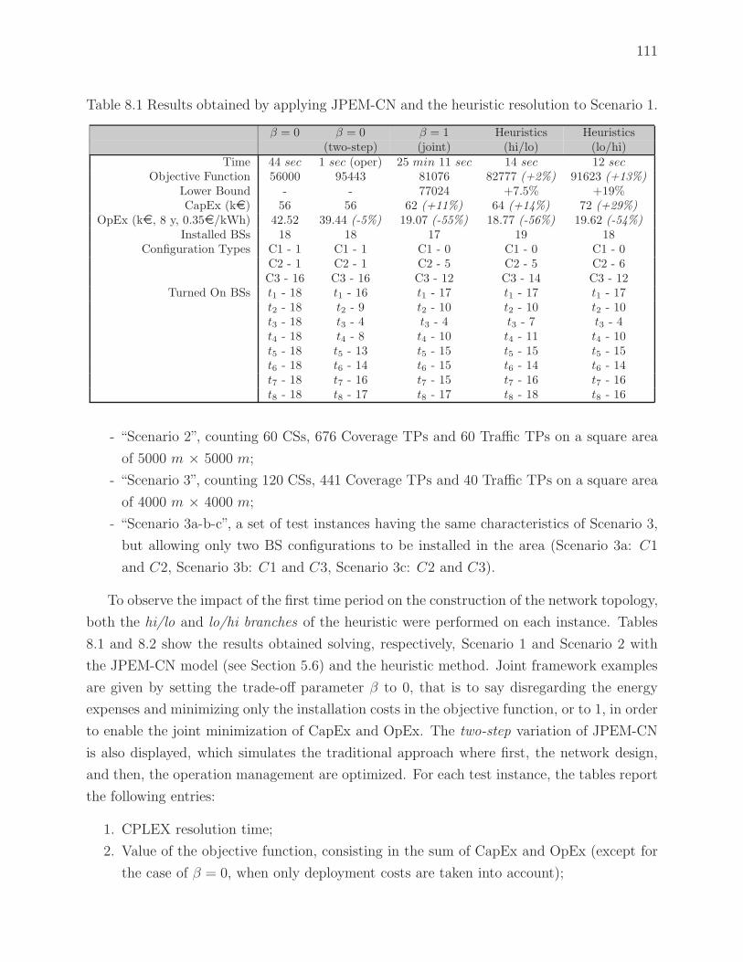
111

Table 8.1 Results obtained by applying JPEM-CN and the heuristic resolution to Scenario 1.

β = 0 β = 0 β = 1 Heuristics Heuristics(two-step) (joint) (hi/lo) (lo/hi)

Time 44 sec 1 sec (oper) 25 min 11 sec 14 sec 12 secObjective Function 56000 95443 81076 82777 (+2%) 91623 (+13%)

Lower Bound - - 77024 +7.5% +19%CapEx (k¤) 56 56 62 (+11%) 64 (+14%) 72 (+29%)

OpEx (k¤, 8 y, 0.35¤/kWh) 42.52 39.44 (-5%) 19.07 (-55%) 18.77 (-56%) 19.62 (-54%)Installed BSs 18 18 17 19 18



- “Scenario 2”, counting 60 CSs, 676 Coverage TPs and 60 Traffic TPs on a square area

of 5000 m × 5000 m;

- “Scenario 3”, counting 120 CSs, 441 Coverage TPs and 40 Traffic TPs on a square area

of 4000 m × 4000 m;

- “Scenario 3a-b-c”, a set of test instances having the same characteristics of Scenario 3,

but allowing only two BS configurations to be installed in the area (Scenario 3a: C1

and C2, Scenario 3b: C1 and C3, Scenario 3c: C2 and C3).

To observe the impact of the first time period on the construction of the network topology,

both the hi/lo and lo/hi branches of the heuristic were performed on each instance. Tables

8.1 and 8.2 show the results obtained solving, respectively, Scenario 1 and Scenario 2 with

the JPEM-CN model (see Section 5.6) and the heuristic method. Joint framework examples

are given by setting the trade-off parameter β to 0, that is to say disregarding the energy

expenses and minimizing only the installation costs in the objective function, or to 1, in order

to enable the joint minimization of CapEx and OpEx. The two-step variation of JPEM-CN

is also displayed, which simulates the traditional approach where first, the network design,

and then, the operation management are optimized. For each test instance, the tables report

the following entries:

1. CPLEX resolution time;

2. Value of the objective function, consisting in the sum of CapEx and OpEx (except for

the case of β = 0, when only deployment costs are taken into account);

112

Table 8.2 Results obtained by applying JPEM-CN and the heuristic resolution to Scenario 2.

β = 0 β = 0 β = 1 Heuristics Heuristics(two-step) (joint) (hi/lo) (lo/hi)

Time 25 sec 1 sec (oper) 1 min 51 sec 7 sec 9 secObjective Function 267000 464801 411013 432570 (+5%) 461838 (+12%)

Lower Bound - - 391952 +10% +18%CapEx (k¤) 267 267 277 (+4%) 300 (+12%) 336 (+26%)

OpEx (k¤, 8 y, 0.35¤/kWh) 202.64 197.80 (-3%) 134.01 (-34%) 132.57 (-35%) 125.84 (-38%)Installed BSs 23 23 30 35 33



3. Percentage difference between the objective function resulting from phase II.II of the

heuristic and the lower bound of the same test instance solved with JPEM-CN by

setting β = 1. Due to the altered nature of the problem when β = 0, in which case

no importance is given to the reduction of the operation energy consumption during

the network design phase, the corresponding lower bounds and respective percentage

differences are not considered;

4. CapEx, expressed in thousands of Euro and corresponding to the value of the first term

of the objective function;

5. OpEx of the network, constituting the second term of the objective function and

calculated over a 8 year period by considering the energy cost for business users of

0.35 ¤/kWh;

6. Number and type of access stations installed in the area;

7. Number of access stations switched on during every time period.

Moreover, percentages in parenthesis refer to the objective function value, installation and op-

erational expenses obtained for the unmanaged minimum cost topology (JPEM-CN,β = 0).

First of all, observe the values of the objective function obtained for Scenario 1 and

Scenario 2 using the hi/lo and lo/hi heuristic resolutions. Comparing these results to the

corresponding values acquired from the JPEM-CN by imposing β = 1, it is evident how

the proposed method provides very good approximations of the solutions computed by the

joint framework. The heuristic objective function value exceeds the joint formulation one

only by 2% and 5% in the hi/lo case for Scenario 1 and 2, while the percentages grow to

113

Figure 8.2 Heuristic method performance: percentage deviation from the lower bound andfrom the joint framework solutions.

13% and 12% when the lo/hi resolution is considered. However, taking into account that

the JPEM-CN instances are solved by setting a 5% gap to optimality, it is fundamental for

the correct evaluation of the heuristic performance to examine the hi/lo and lo/hi results

in correlation to the lower bounds of the β = 1 JPEM-CN solution. Figure 8.2 displays

the percentage deviation of the solutions obtained from the joint and heuristic formulations

from the lower bounds for Scenario 1 and 2. The percentage difference between the heuristic

solutions (dashed lines) and the joint formulation ones (dark gray line) are also reported in the

chart. Showing percentage differences of +7.5% and +10% for Scenario 1 and 2 respectively,

the objective function of the hi/lo branch seems to maintain a closer proximity to the lower

bound of the joint formulation than the lo/hi branch, for which the percentages grow at +19%

and +18%. Extending the analysis to the values of CapEx and OpEx, the heuristic seem

to perform similarly to the original model: in both cases, the initial installation investments

undergo modest increases with respect to the minimum cost topology (+12% and +14%

for the hi/lo, +29% and +26% for the lo/hi) to ensure high energy savings in the network

operation management phase. In most of the examples, the computed OpEx is even lower

than the one calculated by the JPEM-CN with β = 1, indicating that the presented technique

is successfully driven toward the installation of an effective energy-aware network topology.

In this sense, the heuristic seems to reproduce the behavior of the JPEM-CN framework

114

when the trade-off parameter is greater than one, that is, when the operational costs are

given higher weight then the CapEx in the model’s objective function (see Tables 5.3 and 5.4

for a comparison). Now, if the number and types of deployed access devices are considered,

the same tendency to install small and medium size BSs typical of the JPEM-CN is found

again in the heuristic resolution. The choice of the time periods to be examined, as well as

the importance given to the sole energy-aware operation in the first phases of the heuristic

procedure, guarantee a high level of flexibility to the resulting network topology. Lastly, note

that the computational time is of the order of seconds in all cases.

Further results from Scenarios 3 and its variations 3a, 3b and 3c are gathered in Table

8.3. For each instance, the β = 1 JPEM-CN solution is directly compared to the outcomes of

the hi/lo and lo/hi heuristic. Once again, the solving time is reported first, then the value of

the objective function. The lower bound of the solution is displayed for the joint framework

instances, while the difference percentage to the lower bound is calculated for the heuristic

results. Capital and operational expenditures are measured in thousands of Euro; finally, the

number and configuration of the installed devices are presented.

As observed for the previous examples, the heuristic performs very well in terms of cost

values and deployed topology. The objective functions never diverge more than +6% from

the lower bounds of the respective joint problem results; likewise, the heuristic’s CapEx and

OpEx are almost identical or even slightly lower than the ones computed by the original

formulation. No significant differences can be identified between the JPEM-CN and the

heuristic resolutions in the amount or type of installed access stations. On the other hand,

the computational time required by CPLEX to solve some of the instances appears much

higher than in the examples reported in Tables 8.1 and 8.2 for Scenario 1 and Scenario 2.

While the hi/lo branch of the heuristic is able to solve Scenario 3a much faster than the joint

framework (less than 2 minutes, compared to 20 minutes 25 seconds in the JPEM-CN case),

Scenario 3 and 3c seem to be more challenging, requiring respectively almost 17 minutes

and 8 minutes 12 seconds to be solved. Interestingly, the lo/hi branch behaves differently,

showing much lower resolution times for most of the examples.

The outstanding results obtained by testing the heuristic on small scenarios paved the

way to the analysis of bigger instances to measure the performance of the proposed heuristic

procedure when real-size problems are taken into account. In the next Section, new scenarios

are introduced and the heuristic outcomes are presented and described.

115

Table 8.3 Important results obtained applying JPEM-CN (β = 1) and the heuristic resolutionto Scenario 3 and its variations.


Time 2 min 22 sec 20 min 25 sec 17 sec 43 secObjective Function 182379 311288 386516 182966

Lower Bound 176960 295056 384391 177301CapEx (k¤) 136 240 190 137

OpEx (k¤, 8 y, 0.35¤/kWh) 45.38 71.29 196.52 45.97Installed BSs C1 - 0 C1 - 0 C1 - 6 C1 - n.a.

C2 - 12 C2 - 24 C2 - n.a. C2 - 12C3 - 16 C3 - n.a. C3 - 10 C3 - 17

Heuristics (hi/lo):Time 16 min 56 sec 1min 49 sec 3 min 25 sec 8 min 12 sec

Objective Function 182569 (+0.1%) 311432 (+0.04%) 385399 (-0.2%) 183393(+0.2%)Vs. Lower Bound +3% +6% +0.2% +3%

CapEx (k¤) 137 240 (+0%) 189 (-0.5%) 138 (+0.7%)OpEx (k¤, 8 y, 0.35¤/kWh) 45.57 71.43 (+0.2%) 196.40 (+0.1%) 45.39 (-1%)


Heuristics (lo/hi):Time 37 sec 50 sec 2 min 42 sec 26 sec

Objective Function 182393 (+0%) 311577 (+0.1%) 386443 (+0.01%) 181261 (-1%)Vs. Lower Bound +3% +6% +0.5% +2%

CapEx (k¤) 137 240 (+0%) 190 (+0%) 136 (-0.7%)OpEx (k¤, 8 y, 0.35¤/kWh) 45.39 71.58 (+0.4%) 196.44 (+0.1%) 45.26 (-1%)


116

Table 8.4 Parameters used to generate the heuristic test scenarios.

Area (km2) CSs CTPs TTPs Allowed Configurations

Scenario A 6×6 130 961 50 AllScenario B 6×6 200 961 70 AllScenario C 7×7 220 1296 80 AllScenario D 8×8 250 1681 60 AllScenario E 8×8 400 1681 90 AllScenario F 8×8 500 1681 150 AllScenario G 10×10 450 2601 90 AllScenario H 10×10 500 2601 110 AllScenario I 10×10 600 2601 150 AllScenario L 10×10 700 2601 180 AllScenario M 15×15 1000 5576 200 All

8.4 Performance evaluation on real-size test scenarios

The numerical examples presented in Section 8.3 highlighted the heuristic’s capability to

reproduce the behavior of the joint design and energy management problem formulation.

Keeping the computational time low, the approach provides as output a flexible network

topology whose CapEx are only moderately higher than the minimum cost topology ones,

and whose OpEx are similar or lower than the ones computed with the JPEM-CN framework.

At this point, larger test instances need to be generated to observe the performance of the

heuristic and further confirm its validity. To do so, the same instance generator (IG) described

in Section 5.7.1 was used. Eleven test scenarios were created; their names and features are

reported in Table 8.4. As displayed in the table, these scenarios present different values of

coverage area as well as different number of Traffic TPs and CSs. The objective is to measure

the heuristic resolution time in each case, especially when many customers or possible sites

for access devices are considered. If the heuristic will prove to be able to solve real-size

scenarios in a reasonable amount of time, it will be used as a basis to extend the research on

the joint network planning and design concept, up to now impeded by the JPEM-CN model

complexity.

Table 8.5 illustrates the results produced by solving Scenario A to Scenario M. In par-

ticular, for both versions of the heuristic, the table displays the CPLEX resolution time,

the objective function and the values of capital and operational expenditures necessary to

the calculated topology. Also, percentages in parenthesis measure the difference between

the lo/hi and the hi/lo solving time and resulting objective function. At a glance, it can

be noticed that the hi/lo and lo/hi branches perform very similarly in terms of computed

CapEx and OpEx. Nevertheless, the hi/lo version overcomes the lo/hi one in almost all

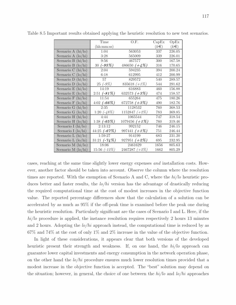
117

Table 8.5 Important results obtained applying the heuristic resolution to new test scenarios.

Time O.F. CapEx OpEx(hh:mm:ss) (k¤) (k¤)

Scenario A (hi/lo) 1:04 563053 337 226.05Scenario A (lo/hi) 3:28 565009 339 226.01Scenario B (hi/lo) 9:56 467577 300 167.58Scenario B (lo/hi) 30 (-95%) 486650 (+4%) 316 170.65Scenario C (hi/lo) 2:04 594235 394 200.24Scenario C (lo/hi) 6:18 612995 412 200.99Scenario D (hi/lo) 57 829572 540 289.57Scenario D (lo/hi) 25 (-9%) 835618 (+1%) 544 291.62Scenario E (hi/lo) 14:19 616883 460 156.88Scenario E (lo/hi) 2:51 (-81%) 632573 (+3%) 474 158.57Scenario F (hi/lo) 11:54 655264 475 180.26Scenario F (lo/hi) 4:02 (-66%) 672758 (+3%) 490 182.76Scenario G (hi/lo) 2:35 1128532 760 368.53Scenario G (lo/hi) 1:20 (-48%) 1152847 (+2%) 783 369.85Scenario H (hi/lo) 4:44 1065544 747 318.54Scenario H (lo/hi) 1:38 (-65%) 1079456 (+1%) 760 319.46Scenario I (hi/lo) 2:13:12 992152 746 246.15Scenario I (lo/hi) 44:25 (-67%) 997441 (+1%) 751 246.44Scenario L (hi/lo) 1:59:27 914199 683 231.20Scenario L (lo/hi) 31:21 (-74%) 927951 (+2%) 695 232.95Scenario M (hi/lo) 18:06 2461629 1656 805.63Scenario M (lo/hi) 15:56 (-12%) 2467287 (+2%) 1662 805.29

cases, reaching at the same time slightly lower energy expenses and installation costs. How-

ever, another factor should be taken into account. Observe the column where the resolution

times are reported. With the exemption of Scenario A and C, where the hi/lo heuristic pro-

duces better and faster results, the lo/hi version has the advantage of drastically reducing

the required computational time at the cost of modest increases in the objective function

value. The reported percentage differences show that the calculation of a solution can be

accelerated by as much as 95% if the off-peak time is examined before the peak one during

the heuristic resolution. Particularly significant are the cases of Scenario I and L. Here, if the

hi/lo procedure is applied, the instance resolution requires respectively 2 hours 13 minutes

and 2 hours. Adopting the lo/hi approach instead, the computational time is reduced by as

67% and 74% at the cost of only 1% and 2% increase in the value of the objective function.

In light of these considerations, it appears clear that both versions of the developed

heuristic present their strength and weakness. If, on one hand, the hi/lo approach can

guarantee lower capital investments and energy consumption in the network operation phase,

on the other hand the lo/hi procedure ensures much lower resolution times provided that a

modest increase in the objective function is accepted. The “best” solution may depend on

the situation; however, in general, the choice of one between the hi/lo and lo/hi approaches

118

should be made by bearing in mind that the main goal of an heuristic method is to obtain a

good solution in a short time.

In order to understand which heuristic procedure should be used based on the charac-

teristics of the scenario of interest, it may be useful to identify the solving time trend in

relation to different parameters. Figure 8.3, Figure 8.4 and Figure 8.5 plot the resolution

times obtained from the hi/lo (circle symbol, subfigures (a)) and the lo/hi (triangle symbol,

subfigures (b)) approaches when Scenarios A to M are ordered by:

- Number of candidate sites in the considered area (Figure 8.3);

- Number of traffic test points in the considered area (Figure 8.4);

- Number of candidate sites per traffic test point (Figure 8.5).

Observe the figures, neglecting for a moment the colored area. The time required by the

heuristic to solve the tested instances seems to be independent by any particular character-

istics. Rather, Scenario I and L, which present similar features in terms of number or CSs

and Traffic TPs, appear to be the outliers, especially if the much lower solution time of the

biggest Scenario M is taken into account. Consider now the light grey area delimited on the

lower side by empty circles or triangles, according to which of the two heuristic resolutions

is examined. To reduce the high computational time of specific scenarios, a gap greater than

zero can be set for the heuristic optimization models. Thus, the empty symbols located in

correspondence of the most time consuming instances report the solving time of the same

scenario when the EM-CN and JPEM-CN incorporated in the heuristic are no longer solved

to optimality, but by setting an optimality gap of 3%. The grey-colored areas underline the

change in the solving time curves when the new time values are considered. Selecting a gap

of 3%, the resolution time of Scenario I is decreased from 2 hours 13 minutes to 1 hour 4

minutes (hi/lo procedure) and from 44 minutes to less than 8 minutes (lo/hi procedure);

the time reduction comes at the modest price of, respectively, +1% and +2% increase in the

objective function value. Similarly, when the optimality gap is set to 3%, Scenario L can be

solved in 45 minutes (vs. almost 2 hours, hi/lo procedure) and 15 minutes (vs. 31 minutes,

lo/hi procedure) with only +2% increase in the objective function in both cases.

On the whole, the developed heuristic approach proved to be effective and rather fast

with most of the tested instances. The availability of two different procedures, the hi/lo

and the lo/hi, allows the user to choose between a more precise outcome or a much lower

computational time. Moreover, to further reduce the solving times, it has been demonstrated

that an optimality gap of 3% can be set to speed up the resolution without significantly

affecting the value of the objective function.

119

CS Number

Com

puta

tiona

l Tim

e (s

)

0 50 100 150 200 250 300 350 400 450 500 600 700 800 900 1000

050

010

0015

0020

0025

0030

0040

0050

0060

0070

0080

00

Results Hi−LoGap 3% for time > 30 min

(a) Hi/Lo resolution.

CS Number

Com

puta

tiona

l Tim

e (s

)

0 50 100 150 200 250 300 350 400 450 500 600 700 800 900 1000

050

010

0015

0020

0025

0030

0040

0050

0060

0070

0080

00

Heuristics Lo−HiGap 3% for time > 30 min

(b) Lo/Hi resolution.

Figure 8.3 Computational time, instances ordered by number of CS.

120

Traffic TP Number

Com

puta

tiona

l Tim

e (s

)

20 40 60 80 100 120 140 160 180 200

050

010

0015

0020

0025

0030

0040

0050

0060

0070

0080

00

Heuristics Hi−LoGap 3% for time > 30 min


Traffic TP Number

Com

puta

tiona

l Tim

e (s

)

20 40 60 80 100 120 140 160 180 200

050

010

0015

0020

0025

0030

0040

0050

0060

0070

0080

00



Figure 8.4 Computational time, instances ordered by number of Traffic TPs.

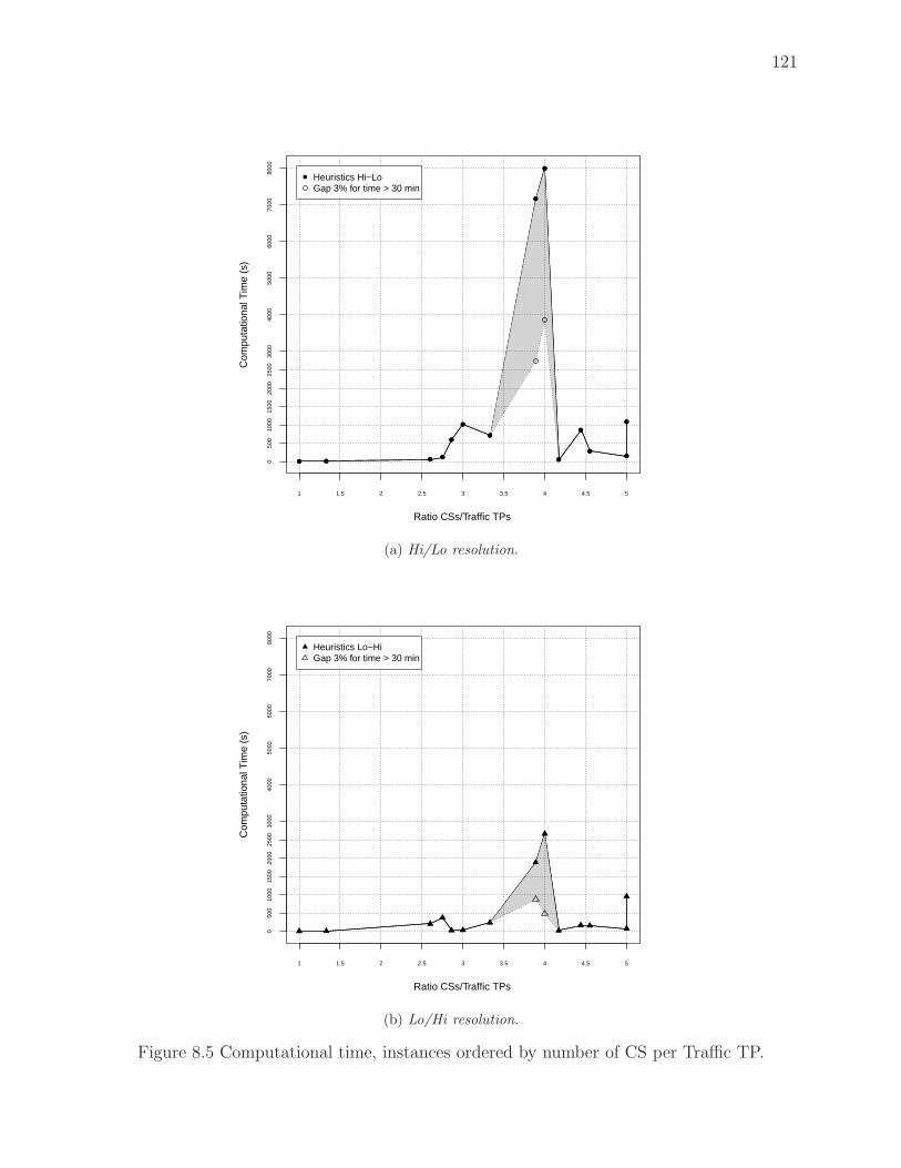
121

Ratio CSs/Traffic TPs

Com

puta

tiona

l Tim

e (s

)

1 1.5 2 2.5 3 3.5 4 4.5 5

050

010

0015

0020

0025

0030

0040

0050

0060

0070

0080

00

Heuristics Hi−LoGap 3% for time > 30 min


Ratio CSs/Traffic TPs

Com

puta

tiona

l Tim

e (s

)

1 1.5 2 2.5 3 3.5 4 4.5 5

050

010

0015

0020

0025

0030

0040

0050

0060

0070

0080

00



Figure 8.5 Computational time, instances ordered by number of CS per Traffic TP.

122

CHAPTER 9

GENERAL DISCUSSION

Legacy wireless access networks (WANs) are typically designed regardless of energy efficiency

issues; the planning objective is to minimize the installation costs while guaranteeing com-

plete area coverage and connection quality in any load condition, especially during peak

traffic periods. In recent years, the rising demand for pervasive mobile communication ac-

cess increased not only the amount of customers to be served, but also the awareness of the

environmental impact. Therefore, if on one hand the capacity of the current networks has

to be upgraded to be able to manage the extra traffic, on the other hand new energy-aware

techniques should to be taken into account and introduced in the regular network functioning.

In this regard, different approaches have been proposed, mainly aiming at powering off un-

necessary access stations during low load periods to reduce the power waste. However, when

cell sleeping procedures are applied to legacy access networks, only minor energy savings can

be obtained: although overprovisioned, such networks are mainly composed by large, high

power access devices that can hardly be turned off due mostly to their wide area coverage.

The research presented in this doctoral thesis originates from these considerations, claim-

ing that an energy-aware network design is the key to obtain an effective energy-aware network

management. In other words, the network can be provided with enough flexibility to follow

the traffic variations only if an energy-aware operation management is considered during

the planning stages. To prove this assertion, the joint planning and energy management

problem (JPEM) was developed and presented in its general characteristics in Chapter 4.

Assuming no pre-existent topology, for the first time in literature the proposed framework

jointly minimizes the capital expenditures (CapEx) related to the network installation and

the operational and management expenditures (OpEx) over the network lifetime in order to

choose the most energy-efficient network deployment in respect of capital investment limita-

tions. Different topologies can be produced by tuning a trade-off parameter, used to regulate

the relative importance of the capital and operational expenses in the objective function.

When the OpEx term is disregarded, the minimum cost topology is obtained; conversely, if

the joint optimization is enabled, the model is forced to reduce not only the capital but also

the operational costs. At the price of modest increases in the CapEx expenses, the resulting

topologies are more flexible, strategically deploying a high number of small and medium size

cells that allow the operation management mechanism to reach significant energy savings.

The proposed formulation has been adapted to two types of wireless access technology.

123

The joint planning and energy management problem for cellular networks (JPEM-CN) is pre-

sented in Chapter 5. Three types of access stations have been made available to be installed.

Numerical results obtained by six test scenarios confirmed that network topologies designed

by taking into account the future power-aware operation reach energy savings of about 60%

with respect to the unmanaged minimum cost topology. To carry out a fair comparison, a

two-step model variation was developed to simulate a more traditional approach where first,

the minimum cost topology is deployed and then, the operation of the installed topology is

managed. As expected, results showed that only limited savings on the order of 5% can be

reached by managing a pre-installed minimum cost topology due to the inflexibility typical of

networks designed ignoring any energy efficiency consideration. A partial covering variation

of the JPEM-CN was proposed to study the model performance when only active customers

in the area have to be provided with network service; this way, access devices covering just

idle users can be put to sleep. Although not applicable in current network architectures, such

a coverage technique would be used in case of a future separation of the signaling and data

network, in which case large, constantly active signaling cells would be responsible for the

total area coverage, while small cells would provide network service only to active customers.

Predictably, the registered energy savings increased, reaching 70% with respect to the mini-

mum cost unmanaged topology and 37% with respect to the total coverage case. Finally, the

last variation examined for the cellular version of the JPEM involves the introduction of a

maximum budget on the capital expenses. The CapEx term in the object function is dropped

while a new set of constraints caps the installation costs to the predetermined limit. The

Budget JPEM-CN, described in Chapter 7, was developed to model possible hard constraints

imposed by the network operator on the network capital investments; results proved that the

variation obtains comparable results to the original formulation in a similar amount of time.

In addition to cellular networks, the joint framework has been adjusted to fit the char-

acteristics of wireless access networks (JPEM-WMN, presented in detail in Chapter 6). The

same joint optimization principles described for cellular networks apply in this case; how-

ever, only two access devices are allowed to be deployed in the area, having same coverage

and capacity capabilities: mesh routers, providing network access for the mesh clients and

connecting to other routers and gateways through point to point links, and mesh access

points, similar to routers but connected directly to the wired backbone. Test results on mesh

scenarios highlighted energy savings around 25% to 30% when the joint framework is used,

compared to the unmanaged minimum cost topology; the lower energy savings observed for

WMNs are due to the limited variety of available access devices and prove once more the

importance of the topology flexibility for an effective power-aware management. Again, a

two-step approach was introduced to fairly evaluate the model performance, showing power

124

reduction of less than 10% in all examples. Moreover, a set of other variations was tested

on the JPEM-WMN. Besides the partial covering problem, which is able to provide energy

savings 9% to 15% higher than the total coverage model, a MAPs only variant was devel-

oped to disable the multi-hop characteristics of mesh networks and replicate the behavior

or a cellular one. An alternative form of JPEM-WMN considers variable capacity for the

backbone wireless links according to the access station mutual distance. Also, in the On/Off

JPEM-WMN formulation presented in Chapter 7, new constraints are added to limit the

number of state changes (from on to off and vice versa) for each access station, the objective

being to preserve the device functionality and reduce the energy waste during the activation

transition.

Finally, an ad hoc heuristic method was developed to obtain faster results and allow the

solution of real size instances. In particular, the heuristic approach was tested on the cellular

network problem, which turned out to be more computationally expensive than the mesh

network counterpart. The idea underlying the proposed technique is that the complexity of

the original JPEM-CN could be highly reduced if an initial topology was provided in input

to the model; therefore, the heuristic computes a partial topology by selecting an energy-

aware BS activation pattern during two specific time periods in the day. Given in input to

the joint framework, the partial topology is integrated and made feasible for the whole day.

When tested on the same toy scenario used for the JPEM-CN, the heuristic showed results

only 2% to 5% higher than the joint framework ones in the best cases, while solving time are

greatly decreased in almost all cases. Eleven additional test instances were generated to assess

the heuristic performance with realistic size examples. The heuristic approach successfully

solved every scenario, whereof the larger one counted 1000 Candidate Sites and 200 Traffic

Test Points. The resolution time overtakes 30 minutes only in two cases, but keeps below 20

minutes for the remaining nine instances. Overall, the developed heuristic proved to be an

effective tool, rather precise and fast in reaching a solution even when large instances were

considered.

125

CHAPTER 10

CONCLUSION

The growing demand for telecommunications services is drawing attention on the current

state of the supporting infrastructure, which needs to be widened and upgraded, as well as

on the ICT sector energy footprint, that can no longer be ignored. On the other hand, from

the mobile operators’ point of view, this uninterrupted spread translates in higher expenses

for the installation and management of new devices. In this context, green networking has

become one of the most actual topics concerning the telecommunications sector. With the aim

of decreasing the energy consumption of current networks, researchers have recently tackled

the energy-aware network design and operation issue for both wired and wireless networks.

However, the relationship between network planning and operation energy efficiency is an

aspect of the problem so far disregarded.

Focusing on wireless systems, the research project tried to fill this gap by demonstrating

the influence of the network topology on the effectiveness of a power-aware network manage-

ment. In particular, the network flexibility, defined as the capacity of the topology to adapt

to the traffic demand variation in time and space, is claimed to be the key requirement to

enable high energy savings in the management phase. In order to prove these assertions, the

joint planning and energy management problem (JPEM) was developed. The mathematical

framework jointly minimizes the network installation expenses and its expected operational

costs. By regulating the relative importance of the CapEx and OpEx terms through a trade-

off parameter, multiple network topologies are obtained. When the power expenditures are

ignored, the minimum installation cost network is deployed; on the other hand, when a

modest increase in the capital investments are tolerated, the JPEM computes the best net-

work topology based on its energy savings potentials in the operation stage. Therefore, the

proposed optimization tool offers the opportunity to design the network configuration that

best complies with the different cost requirements and, at the same time, shows the possible

advantages attainable from a cell sleeping mechanism applied to the selected topology.

10.1 Achievements of the doctoral research

During the doctoral research period, the following objectives were accomplished.

126

10.1.1 Joint Planning and Energy Management of Cellular Networks

The JPEM framework was adapted to the cellular access technology (JPEM-CN). In order

to test the joint formulation, a daily traffic variation pattern was defined; also, believing

that the availability of different size cells is fundamental to follow the traffic fluctuations

and maximize the energy savings, three access station categories (macro, micro and pico

cells) were allowed in cellular instances. Results computed on LTE instances showed that,

when the OpEx are ignored during the planning stage, the installed topologies are in general

composed by the minimum number of cells; the network structure presents a substantial

group of pico and micro access stations, while macro cells are deployed in smaller number.

The coexistence of a mixture of different cells could lead to believe in the effectiveness of an

energy-aware management of the network. However, the opposite effect was verified: when a

power-efficient operation is applied to the minimum cost topology, negligible savings around

5% can be reached compared to the non managed network operation. The situation changes

when CapEx and OpEx are jointly minimized. By increasing the influence of the energy

expenditures, more access stations are deployed. Micro cells, providing the lower power

consumption per unit of covered area, are the ones experiencing the highest increase as the

OpEx acquire more importance in the model objective function. The number of pico cells

slightly grows, while macro cells are reduced or excluded from the topology. As a result, the

network energy consumption is decreased of about 35% to 60%, depending on the considered

scenario and on the trade-off value, at the cost of an increment of CapEx lower than 15%.

10.1.2 Joint Planning and Energy Management of Wireless Mesh Networks

The JPEM was reformulated to adjust to wireless mesh access technology (JPEM-WMN).

As in the cellular case, traffic variations during the day were considered; however, only

two types of same size access devices (router or gateway) can compose a mesh topology.

Numerical results were obtained through a set of Wi-Fi mesh test instances. Here, the effect

of the proposed joint framework is remarkable but weakened by the reduced choice in terms of

access station types; nonetheless, power savings between 20% and 30% are achieved for most

test scenarios, compared to savings below 10% reached when the minimum cost topology is

managed. Once again, when OpEx are given more weight, the number of installed devices

increase without noticeable difference between the routers’ and gateways’ growth rate.

10.1.3 Joint Planning and Energy Management with Partial Area Coverage

A partial coverage variation of the joint framework was developed. This way, network service

is provided to active customers only, while access stations having only idle users in their

127

coverage radius can be put to sleep. The model was tested on both cellular and wireless mesh

access networks. Results highlighted a further decrease in the network power consumption,

which reaches almost -70% (-25% to -35% if compared to the savings achieved with the original

formulation) in the cellular examples. Conversely, moderate improvements are experimented

for the mesh test scenarios, whose power consumption reduction fluctuates between 9% and

15% with respect to the original JPEM results.

10.1.4 Variations of the Joint Planning and Energy Management Frameworks

Other modifications to the JPEM framework were experimented. Considering the JPEM-CN,

a budget limit was introduced to cap the capital costs to a pre-determined amount, while

only OpEx were minimized in the objective function. The Budget JPEM-CN model proved to

be slightly less performant and more computationally complex than the original formulation,

even though high energy saving between 45% and 55% are still reached for all the tested

scenarios. As far as the JPEM-WMN is concerned, a modified version considered the insertion

of a limitation on the number of device on/off state transitions, in order to reduce the energy

consumed in the wake-up process. Predictably, setting the maximum transition number at one

moderately increased the network energy consumption; in comparison, when access devices

are allowed to freely change their state, additional 5% to 9% power saving are achieved.

Other JPEM-WMN modifications involve the simulation of the cellular network behavior, by

forbidding the installation of mesh routers and thus eliminating the typical mesh network

multi-hop capability, and the introduction of variability in the backbone link capacity.

10.1.5 Heuristic Resoution

An heuristic procedure was developed to obtain results in a short amount of time and allow the

resolution of real-size scenarios. Through the analysis of the BS activation pattern during the

daily peak and off-peak time periods, a partial topology is provided as input to the JPEM-CN

and integrated to form a feasible solution. Numerical tests on small cellular scenarios showed

that the heuristic approach is close to the JPEM-CN framework behavior, producing as

output objective function values only 2% to 5% greater than the joint formulation ones.

Real-size instances were successfully solved with two variations of the same heuristic: in one

case, better final solutions were provided while, in the other case, the resolution time was

strongly reduced. Generally, the heuristic proved to be effective and fast in solving most of

the test instances; in particular, if an optimality gap of 3% is set when the biggest scenarios

are considered, the solution time never exceeds the hour.

128

10.2 Future developments

As regards future work, several refinements of the presented results are possible. Even though

the JPEM focuses on a cell sleeping energy saving mechanism, other operational issues could

be considered as, for example, on-line antenna tilting or cell coverage zooming. An extremely

interesting future development would consider access devices powered by renewable energy

(solar or wind, for example) or by a combination of clean energies and a backup battery.

User mobility could also be taken into account by developing a real time on-line operation

management model.

A very innovative continuation of the research project would consists in the further ex-

ploration of the partial coverage opportunity for data networks (as in Capone et al., 2012a).

The main idea is that of allowing independent network configurations for data and signaling

systems. Coverage gaps in inactive areas are permitted for the data network; on the other

hand, the signaling network, which is static and guarantees full coverage to the service area,

is able to detect new active users and provide them with network capacity by dynamically

switching on data devices (if necessary). The interaction of signaling and data systems would

be studied, as well as the effective power consumption and offered connection quality.

129

BIBLIOGRAPHY

AKYILDIZ, I., WANG, X. and WANG, W. (2005). Wireless mesh networks: a survey.

Computer Networks, 47, 445–487.

ALLMAN, M., CHRISTENSEN, K., NORDMAN, B. and PAXSON, V. (2007). Enabling

an energy-efficient future internet through selectively connected end systems. 6th ACM

Workshop on Hot Topics in Networks (HotNets), 2007. 1–6.

AMALDI, E., CAPONE, A., CESANA, M., FILIPPINI, I. and MALUCELLI, F. (2008).

Optimization models and methods for planning wireless mesh networks. Computer Networks,

52, 2159–2171.

AMALDI, E., CAPONE, A. and MALUCELLI, F. (2003). Planning UMTS base station

location: Optimization models with power control and algorithms. IEEE Transaction on

Wireless Communications, 2, 932–952.

ANANTHANARAYANAN, G. and KATZ, R. H. (2008). Greening the switch. Conference

on Power Aware Computing and Systems, 2008. USENIX Association, Berkeley, CA, USA,

HotPower’08, 7–7.

BADIC, B., O’FARRRELL, T., LOSKOT, P. and HE, J. (2009). Energy efficient radio

access architectures for green radio: Large versus small cell size deployment. 70th IEEE

Vehicular Technology Conference (VTC), 2009. 1–5.

BALDI, M. and OFEK, Y. (2009). Time for a “greener” Internet. IEEE International

Conference on Communications (ICC), 2009. 1–6.

BIANZINO, A., CHAUDET, C., ROSSI, D. and ROUGIER, J. (2012). A survey of green

networking research. IEEE Communications Surveys Tutorials, 14, 3–20.

BLUME, O., ZELLER, D. and BARTH, U. (2010). Approaches to energy efficient wireless

access networks. 4th IEEE International Symposium on Communications, Control and

Signal Processing (ISCCSP), 2010. 1–5.

BOIARDI, S., CAPONE, A. and SANSO, B. (2012a). Energy-aware planning and manage-

ment of wireless mesh networks. IEEE Global Communications Conference (GLOBECOM),

2012. 3049–3055.

130

BOIARDI, S., CAPONE, A. and SANSO, B. (2012b). Joint design and management of

energy-aware mesh networks. Ad Hoc Networks, 10, 1482 – 1496.

BOIARDI, S., CAPONE, A. and SANSO, B. (2012c). Radio planning of energy-efficient cel-

lular networks. 21st International Conference on Computer Communications and Networks

(ICCCN), 2012. 1–7.

BOIARDI, S., CAPONE, A. and SANSO, B. (2013). Radio planning of energy-aware cellular

networks. Computer Networks, 57, 2564 – 2577.

BOIARDI, S., CAPONE, A. and SANSO, B. (2014). Planning for energy-aware wireless

networks. IEEE Communications Magazine, 52, 156–162.

BOIARDI, S., CAPONE, C. and SANSO, B. (2010). Radio planning

of energy-aware cellular networks. Optimization Online. Available at

http://www.optimization-online.org/DB_HTML/2010/11/2789.html.

BOLLA, R., BRUSCHI, R., DAVOLI, F. and CUCCHIETTI, F. (2011a). Energy efficiency

in the future internet: a survey of existing approaches and trends in energy-aware fixed

network infrastructures. IEEE Communications Surveys & Tutorials, 13, 223–244.

BOLLA, R., DAVOLI, F., BRUSCHI, R., CHRISTENSEN, K., CUCCHIETTI, F. and

SINGH, S. (2011b). The potential impact of green technologies in next-generation wireline

networks: Is there room for energy saving optimization? IEEE Communications Magazine,

49, 80–86.

BOSIO, S., CAPONE, A. and CESANA, M. (2007). Radio planning of wireless local area

networks. IEEE/ACM Transactions on Networking, 15, 1414–1427.

CAPONE, A., FILIPPINI, I., GLOSS, B. and BARTH, U. (2012a). Rethinking cellular

system architecture for breaking current energy efficiency limits. IEEE Sustainable Internet

and ICT for Sustainability (SustainIT), 2012. IEEE, 1–5.

CAPONE, A., MALANDRA, F. and SANSO, B. (2012b). Energy savings in wireless mesh

networks in a time-variable context. Mobile Networks and Applications, 17, 298–311.

CHANG, C.-Y., LIAO, W. and SHAN SHIU, D. (2012). On the coverage preservation prob-

lem in green cellular networks. IEEE Global Communications Conference (GLOBECOM),

2012. 3496–3501.

CHEN, Y. and TSAI, S. (2010). Optimal provisioning of resource in a cloud service. Inter-

national Journal of Computer Science, 7, 95–96.

http://www.optimization-online.org/DB_HTML/2010/11/2789.html

131

CHEN, Y., ZHANG, S. and XU, S. (2010). Characterizing energy efficiency and deploy-

ment efficiency relations for green architecture design. IEEE International Conference on

Communications Workshops (ICC), 2010. IEEE, 1–5.

CHEN, Y., ZHANG, S., XU, S. and LI, G. Y. (2011). Fundamental trade-offs on green

wireless networks. IEEE Communications Magazine, 49, 30–37.

CHIARAVIGLIO, L., CIULLO, D., KOUTITAS, G., MEO, M. and TASSIULAS, L. (2012).

Energy-efficient planning and management of cellular networks. 9th IEEE Annual Confer-

ence on Wireless On-demand Network Systems and Services (WONS), 2012. 159–166.

CHIARAVIGLIO, L., CIULLO, D., MEO, M., MARSAN, M. A. and TORINO, I. (2008a).

Energy-aware UMTS access networks. IEEE W-GREEN, 2008. 1–8.

CHIARAVIGLIO, L., MELLIA, M. and NERI, F. (2008b). Energy-aware networks: Reduc-

ing power consumption by switching off network elements. FEDERICA-Phosphorus tutorial

and workshop (TNC), 2008.

CHRISTENSEN, K., REVIRIEGO, P., NORDMAN, B., BENNETT, M., MOSTOWFI, M.

and MAESTRO, J. (2010). IEEE 802.3az: the road to energy efficient ethernet. IEEE

Communications Magazine, 48, 50–56.

CLAUSSEN, H., HO, L. T. and PIVIT, F. (2008). Effects of joint macrocell and residential

picocell deployment on the network energy efficiency. 19th IEEE International Symposium

on Personal, Indoor and Mobile Radio Communications (PIMRC), 2008. 1–6.

CORREIA, L. M., ZELLER, D., BLUME, O., FERLING, D., JADING, Y., GODOR, I.,

AUER, G. and VAN DER PERRE, L. (2010). Challenges and enabling technologies for

energy aware mobile radio networks. IEEE Communications Magazine, 48, 66–72.

CPLEX, I.B.M. (2010). IBM ILOG AMPL CPLEX 12.2 user’s guide.

EISENBLATTER, A. and GEERD, H. (2006). Wireless network design: solution-oriented

modeling and mathematical optimization. IEEE Wireless Communications, 13, 8–14.

EISENBLATTER, A., GEERDES, H.-F., GROSS, J., PUNAL, O. and SCHWEIGER, J.

(2010). A two-stage approach to wlan planning: Detailed performance evaluation along the

pareto frontier. 8th International Symposium on Modeling and Optimization in Mobile, Ad

Hoc and Wireless Networks (WiOpt), 2010. 227–236.

132

FENG, D., JIANG, C., LIM, G., CIMINI JR, L. J., FENG, G. and LI, G. Y. (2013).

A survey of energy-efficient wireless communications. IEEE Communications Surveys &

Tutorials, 15, 167–178.

GONZALEZ-BREVIS, P., GONDZIO, J., FAN, Y., POOR, H. V., THOMPSON, J.,

KRIKIDIS, I. and CHUNG, P.-J. (2011). Base station location optimization for mini-

mal energy consumption in wireless networks. 73rd IEEE Vehicular Technology Conference

(VTC), 2011. 1–5.

Greentouch (2010). Greentouch consortium. http://www.greentouch.org/.

GRUBER, M., BLUME, O., FERLING, D., ZELLER, D., IMRAN, M. and STRINATI, E.

(2009). EARTH – energy aware radio and network technologies. 20th IEEE International

Symposium on Personal, Indoor and Mobile Radio Communications (PIMRC), 2009. 1–5.

GUNARATNE, C., CHRISTENSEN, K., NORDMAN, B. and SUEN, S. (2008). Reducing

the energy consumption of ethernet with adaptive link rate (alr). IEEE Transactions on

Computers, 57, 448–461.

GUNARATNE, C., CHRISTENSEN, K. and SUEN, S. W. (2006). Ngl02-2: Ethernet adap-

tive link rate (ALR): Analysis of a buffer threshold policy. IEEE Global Telecommunications

Conference (GLOBECOM), 2006. IEEE, 1–6.

GUO, W. and O’FARRELL, T. (2011). Green cellular network: Deployment solutions,

sensitivity and tradeoffs. 7th IEEE Conference on Wireless Advanced (WiAd), 2011. 42–47.

GUPTA, M., GROVER, S. and SINGH, S. (2004). A feasibility study for power management

in LAN switches. 12th IEEE International Conference on Network Protocols (ICNP), 2004.

361–371.

GUPTA, M. and SINGH, S. (2003). Greening of the internet. ACM Conference on Ap-

plications, Technologies, Architectures, and Protocols for Computer Communications, 2003.

19–26.

GUPTA, M. and SINGH, S. (2007). Using low-power modes for energy conservation in

ethernet LANs. IEEE Conference on Computer Communications (INFOCOM), 2007. vol. 7,

2451–55.

HAN, C., HARROLD, T., ARMOUR, S., KRIKIDIS, I., VIDEV, S., GRANT, P. M., HAAS,

H., THOMPSON, J. S., KU, I., WANG, C.-X. ET AL. (2011). Green radio: radio techniques

to enable energy-efficient wireless networks. IEEE Communications Magazine, 49, 46–54.

http://www.greentouch.org/

133

HASAN, Z., BOOSTANIMEHR, H. and BHARGAVA, V. K. (2011). Green cellular net-

works: A survey, some research issues and challenges. IEEE Communications Surveys &

Tutorials, 13, 524–540.

HATA, M. (1980). Empirical formula for propagation loss in land mobile radio services.

IEEE Transactions on Vehicular Technology, 29, 317–325.

HE, B., XIE, B. and AGRAWAL, D. P. (2007). Optimizing the internet gateway deployment

in a wireless mesh network. IEEE International Conference on Mobile Ad Hoc and Sensor

Systems (MASS), 2007. 1–9.

HEEGAARD, P. (2007). Empirical observations of traffic patterns in mobile and ip tele-

phony. Next Generation Teletraffic and Wired/Wireless Advanced Networking, 26–37.

HOLMA, H. and TOSKALA, A. (2009). LTE for UMTS-OFDMA and SC-FDMA based

radio access. John Wiley & Sons.

HURLEY, S. (2002). Planning effective cellular mobile radio networks. IEEE Transactions

on Vehicular Technology, 51, 243–253.

IMRAN, M. A. (2011). Energy efficiency analysis of the reference systems, areas of improve-

ments and target breakdown. Technical report.

ISMAIL, M. and ZHUANG, W. (2011). Network cooperation for energy saving in green

radio communications. IEEE Wireless Communications, 18, 76–81.

JARDOSH, A. P., IANNACCONE, G., PAPAGIANNAKI, K. and VINNAKOTA, B. (2007).

Towards an energy-star WLAN infrastructure. 8th IEEE Workshop on Mobile Computing

Systems and Applications (HotMobile), 2007. 85–90.

JARDOSH, A. P., PAPAGIANNAKI, K., BELDING, E. M., ALMEROTH, K. C., IAN-

NACCONE, G. and VINNAKOTA, B. (2009). Green WLANs: on-demand WLAN infras-

tructures. Mobile Networks and Applications, 14, 798–814.

JOHANSSON, K., FURUSKAR, A., KARLSSON, P. and ZANDER, J. (2004). Relation

between base station characteristics and cost structure in cellular systems. 15th IEEE In-

ternational Symposium on Personal, Indoor and Mobile Radio Communications (PIMRC),

2004. vol. 4, 2627–2631.

JONES, C. E., SIVALINGAM, K. M., AGRAWAL, P. and CHEN, J. C. (2001). A survey

of energy efficient network protocols for wireless networks. Wireless Networks, 7, 343–358.

134

KARL, H. ET AL. (2003). An overview of energy-efficiency techniques for mobile commu-

nication systems. Technical report.

KOUTITAS, G. and DEMESTICHAS, P. (2010). A review of energy efficiency in telecom-

munication networks. Telfor journal, 2, 2–7.

LEE, S., SEO, S. and GOLMIE, N. (2005). An efficient power-saving mechanism for inte-

gration of wlan and cellular networks. IEEE Communications Letters, 9, 1052–1054.

LISTER, D. (2009). An operator’s view on green radio. GreenComm, Keynote Speech.

LITJENS, R. and JORGUSESKI, L. (2010). Potential of energy-oriented network optimi-

sation: Switching off over-capacity in off-peak hours. 21st IEEE International Symposium

on Personal Indoor and Mobile Radio Communications (PIMRC), 2010. 1660–1664.

LORINCZ, J., CAPONE, A. and BEGUSIC, D. (2010). Optimized network management

for energy savings of wireless access networks. Computer Networks, 55, 514–540.

LOUHI, J. T. (2007). Energy efficiency of modern cellular base stations. 29th International

Telecommunications Energy Conference (INTELEC), 2007. 475–476.

MARSAN, M. A., CHIARAVIGLIO, L., CIULLO, D. and MEO, M. (2009). Optimal energy

savings in cellular access networks. IEEE International Conference on Communications

(ICC) Workshops, 2009. 1–5.

MARSAN, M. A., CHIARAVIGLIO, L., CIULLO, D. and MEO, M. (2010). A simple

analytical model for the energy-efficient activation of access points in dense wlans. 1st ACM

International Conference on Energy-Efficient Computing and Networking, 2010. 159–168.

MARSAN, M. A., CHIARAVIGLIO, L., CIULLO, D. and MEO, M. (2013). On the ef-

fectiveness of single and multiple base station sleep modes in cellular networks. Computer

Networks, 57, 3276–3290.

MARSAN, M. A. and MEO, M. (2010). Energy efficient management of two cellular access

networks. ACM SIGMETRICS Performance Evaluation Review. vol. 37, 69–73.

MATHAR, R. and NIESSEN, T. (2000). Optimum positioning of base stations for cellular

radio networks. Wireless Networks, 6, 421–428.

MELLAH, H. and SANSO, B. (2009). Review of facts, data and proposals for a greener

internet. 6th International Conference on Broadband Communications, Networks, and Sys-

tems (BROADNETS), 2009. 1–5.

135

MINAMI, M. and MORIKAWA, H. (2008). Some open challenges for improving the energy

efficiency of the internet. 3rd International Conference on Future Internet (CFI), 2008.

PRIES, R., WAMSER, F., STAEHLE, D., HECK, K. and TRAN-GIA, P. (2009). On traffic

characteristics of a broadband wireless internet access. 5th Euro-NGI Conference on Next

Generation Internet Networks. IEEE Press, 184–190.

QI, Y., IMRAN, M. and TAFAZOLLI, R. (2010). On the energy aware deployment strategy

in cellular systems. 21st IEEE International Symposium on Personal, Indoor and Mobile

Radio Communications Workshops (PIMRC), 2010. 363–367.

QIU, L., CHANDRA, R., JAIN, K. and MAHDIAN, M. (2004). Optimizing the placement

of integration points in multi-hop wireless networks. International Conference on Network

Protocols (ICNP), 2004. vol. 4.

RAMACHANDRAN, K., BUDDHIKOT, M., CHANDRANMENON, G., MILLER, S.,

BELDING-ROYER, E. and ALMEROTH, K. (2005). On the design and implementation

of infrastructure mesh networks. IEEE Workshop on Wireless Mesh Networks (WiMesh),

2005. 4–15.

RICHTER, F., FEHSKE, A. J. and FETTWEIS, G. P. (2009). Energy efficiency aspects of

base station deployment strategies for cellular networks. 70th IEEE International Confer-

ence on Vehicular Technology (VTC), 2009. 1–5.

ROBINSON, J., UYSAL, M., SWAMINATHAN, R. and KNIGHTLY, E. (2008). Adding

capacity points to a wireless mesh network using local search. 27th IEEE Conference on

Computer Communications (INFOCOM), 2008.

SAMA, M., GUPTA, A., AFIFI, H., GENET, M. and JOUABER, B. (2012). Energy saving

by base station pooling: A signaling framework. Wireless Days (WD), 2012 IFIP. 1–7.

SON, K., OH, E. and KRISHNAMACHARI, B. (2011). Energy-aware hierarchical cell

configuration: from deployment to operation. 21st IEEE Conference on Computer Commu-

nications (INFOCOM), 2011. 289–294.

THE CLIMATE GROUP (2008). SMART 2020: Enabling the low carbon economy in the

information age. 2010 State of Green Business.

THE GSMA ASSOCIATION (2009). Green power for mobile: Top ten findings.

136

TIPPER, D., REZGUI, A., KRISHNAMURTHY, P. and PACHARINTANAKUL, P. (2010).

Dimming cellular networks. IEEE Global Telecommunications Conference (GLOBECOM),

2010. 1–6.

WANG, J., XIE, B., CAI, K. and AGRAWAL, D. P. (2007). Efficient mesh router placement

in wireless mesh networks. IEEE International Conference on Mobile Ad Hoc and Sensor

Systems (MASS), 2007. IEEE, 1–9.

WANG, X., KRISHNAMURTHY, P. and TIPPER, D. (2012a). Cell sleeping for energy

efficiency in cellular networks: Is it viable? IEEE Wireless Communications and Networking

Conference (WCNC), 2012. 2509–2514.

WANG, X., VASILAKOS, A. V., CHEN, M., LIU, Y. and KWON, T. T. (2012b). A survey

of green mobile networks: Opportunities and challenges. Mobile Networks and Applications,

17, 4–20.

WENG, X., CAO, D. and NIU, Z. (2011). Energy-efficient cellular network planning under

insufficient cell zooming. 73rd IEEE Vehicular Technology Conference (VTC), 2011. 1–5.

ZEADALLY, S., KHAN, S. U. and CHILAMKURTI, N. (2012). Energy-efficient networking:

past, present, and future. The Journal of Supercomputing, 62, 1093–1118.

ZHANG, F., TODD, T. D., ZHAO, D. and KEZYS, V. (2006). Power saving access points

for IEEE 802.11 wireless network infrastruc ture. IEEE Transactions on Mobile Computing,

144–156.

ZHOU, S., GONG, J., YANG, Z., NIU, Z. and YANG, P. (2009). Green mobile access

network with dynamic base station energy saving. ACM International Conference on Mobile

Computing and Networking, 2009. vol. 9, 10–12.

Radio Planning and Management of Energy-Efficient Wireless ... · RADIO PLANNING AND MANAGEMENT OF...

Documents

Transcript of Radio Planning and Management of Energy-Efficient Wireless ... · RADIO PLANNING AND MANAGEMENT OF...