1

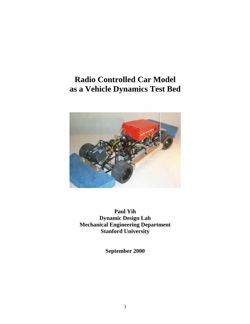
Radio Controlled Car Model as a Vehicle Dynamics Test Bed

Paul Yih Dynamic Design Lab

Mechanical Engineering Department Stanford University

September 2000

2

Table of Contents

I. Overview 3 II. Background 3

III. Mechanical Hardware 4 IV. Electrical Hardware 5 V. Software 6

VI. Applications 9 VII. Work in Progress 12

VIII. Acknowledgments 13 Appendix A: Single board computer setup procedure 14 Appendix B: Code generation with Real-Time Workshop 15 Appendix C: RC car operating procedure 16 Appendix D: Sample data test data 19 Appendix E: Circuit diagram 21 Appendix F: Radio interface circuit board 22 Appendix G: I/O pinouts for radio interface board 23 Appendix H: Sensor interface circuit board 24 Appendix I: I/O pinouts for sensor interface board 25 Appendix J: Measuring pulse width with a PIC 26 Appendix K: Counting pulses with a PIC 27 Appendix L: Simulink m-file 28 Appendix M: Device drivers:

vsbcrad.c vsbcser.c vsbc6ad.c vsbcenc.c

29 31 33 36

Appendix N: PIC code: radio.txt encoder.txt

39 42

Appendix O: List of suppliers 45 Appendix P: Data sheets 47

3

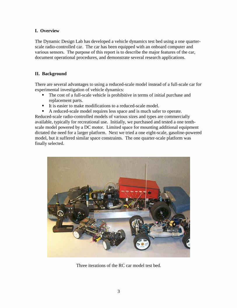
I. Overview The Dynamic Design Lab has developed a vehicle dynamics test bed using a one quarter-scale radio-controlled car. The car has been equipped with an onboard computer and various sensors. The purpose of this report is to describe the major features of the car, document operational procedures, and demonstrate several research applications. II. Background There are several advantages to using a reduced-scale model instead of a full-scale car for experimental investigation of vehicle dynamics: ! The cost of a full-scale vehicle is prohibitive in terms of initial purchase and

replacement parts. ! It is easier to make modifications to a reduced-scale model. ! A reduced-scale model requires less space and is much safer to operate.

Reduced-scale radio-controlled models of various sizes and types are commercially available, typically for recreational use. Initially, we purchased and tested a one tenth-scale model powered by a DC motor. Limited space for mounting additional equipment dictated the need for a larger platform. Next we tried a one eight-scale, gasoline-powered model, but it suffered similar space constraints. The one quarter-scale platform was finally selected.

Three iterations of the RC car model test bed.

4

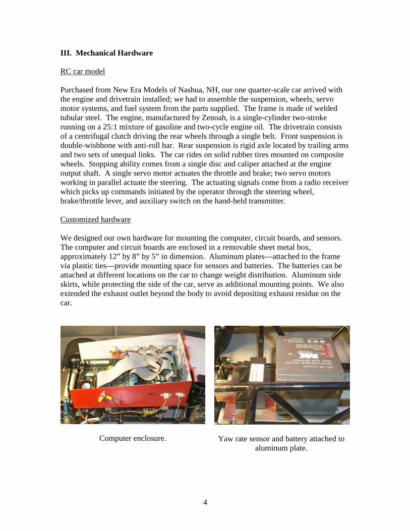
III. Mechanical Hardware RC car model Purchased from New Era Models of Nashua, NH, our one quarter-scale car arrived with the engine and drivetrain installed; we had to assemble the suspension, wheels, servo motor systems, and fuel system from the parts supplied. The frame is made of welded tubular steel. The engine, manufactured by Zenoah, is a single-cylinder two-stroke running on a 25:1 mixture of gasoline and two-cycle engine oil. The drivetrain consists of a centrifugal clutch driving the rear wheels through a single belt. Front suspension is double-wishbone with anti-roll bar. Rear suspension is rigid axle located by trailing arms and two sets of unequal links. The car rides on solid rubber tires mounted on composite wheels. Stopping ability comes from a single disc and caliper attached at the engine output shaft. A single servo motor actuates the throttle and brake; two servo motors working in parallel actuate the steering. The actuating signals come from a radio receiver which picks up commands initiated by the operator through the steering wheel, brake/throttle lever, and auxiliary switch on the hand-held transmitter. Customized hardware We designed our own hardware for mounting the computer, circuit boards, and sensors. The computer and circuit boards are enclosed in a removable sheet metal box, approximately 12” by 8” by 5” in dimension. Aluminum plates—attached to the frame via plastic ties—provide mounting space for sensors and batteries. The batteries can be attached at different locations on the car to change weight distribution. Aluminum side skirts, while protecting the side of the car, serve as additional mounting points. We also extended the exhaust outlet beyond the body to avoid depositing exhaust residue on the car.

Computer enclosure.

Yaw rate sensor and battery attached to aluminum plate.

5

Hall effect sensor mounted to aluminum side skirt.

Custom-made exhaust pipe.

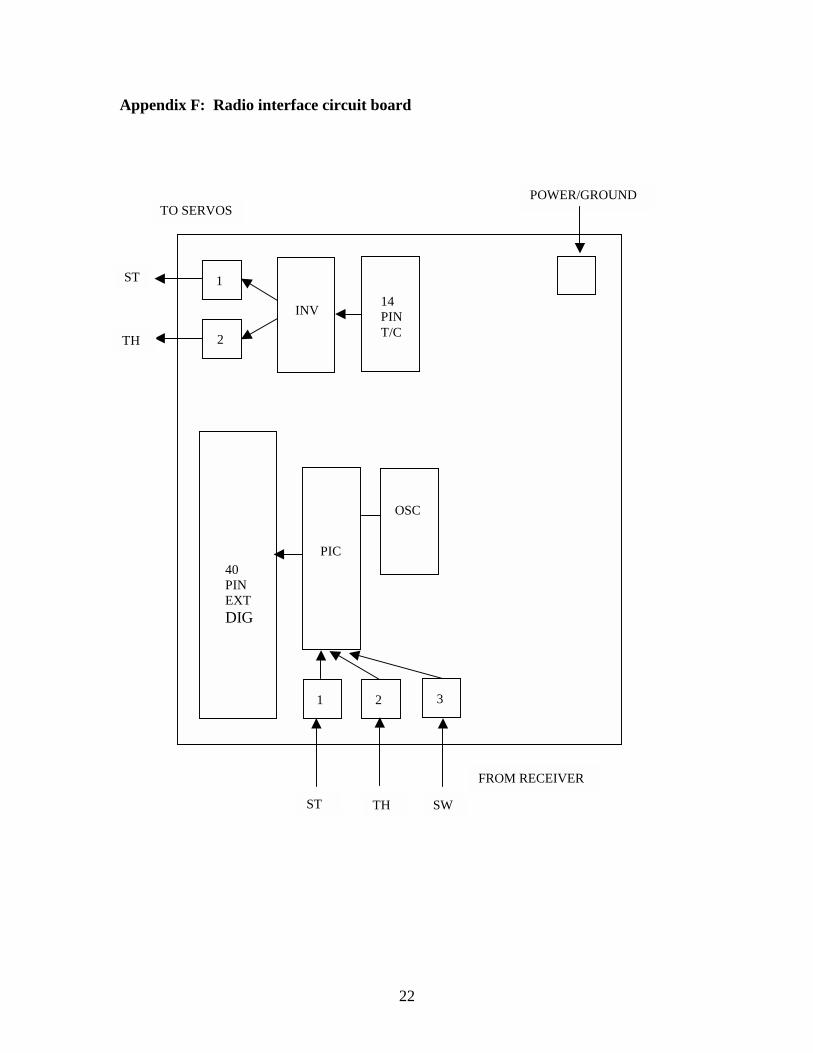
IV. Electrical Hardware Single board computer To make the car useful for dynamics research, we installed an onboard computer system which gives us the ability to monitor vehicle behavior and eventually implement our own control systems. The single board computer from VersaLogic features a 300 MHz AMD K6 processor, bootable Disk On Chip memory device, 16 digital input/output ports, 8 analog input/output ports, and 5 timer/counter ports. We added 16 external analog and digital input/output ports through the PC/104 expansion module. Initial setup procedures for the single board computer are listed in Appendix A. The computer interfaces with the radio receiver, servo motors, and sensors through two separate circuit boards which are explained below. A diagram of the entire circuit is found in Appendix E. Radio interface circuit The radio interface board (Appendix F) contains circuitry to intercept and interpret the radio signals from the receiver and send modified (or unmodified) signals to the servo motors. A PIC programmable microcontroller continuously monitors each of the three receiver channels corresponding to the steering, brake/throttle, and auxiliary switch. The single board computer receives information from the PIC through the external digital I/O ports (Appendix G). After recording and processing the data, the computer sends modified (or unmodified) signals to the steering and brake/throttle servo motors through the timer/counter ports. The connectors are designed so that each of the receiver channels can be connected directly to the servo motors to bypass the computer. In this mode the computer does not record radio signal data.

6

Sensor interface circuit The sensor interface board (Appendix H) provides power to and receives signals from all of the car’s sensors. Thus far we have installed the following sensors: angular rate sensor, two-axis accelerometer, and wheel speed sensor. The output of the angular rate sensor—which measures the yaw rate of the car—is a voltage level proportional to the yaw rate. The accelerometer measures lateral and longitudinal acceleration; its duty cycle output is converted into an analog signal by low-pass filtering and then buffered before feeding into the analog I/O of the computer (Appendix I). Buffering the signal is necessary to prevent the input port’s current draw from altering the signal voltage level. The wheel speed sensor consists of a hall effect gear tooth sensor with pull-up resistor and a ferrous metal gear mounted to the engine output shaft. Each passing of a gear tooth generates a square pulse in the sensor output; the frequency of the pulses corresponds to shaft rotational speed. A PIC microcontroller keeps count of the pulses and sends this information to the computer through the digital I/O ports. Power All of the car’s electronics except for the servo motors and radio receiver run on 5 volts DC. To supply enough current to the computer, which draws over 3 amps, we step the voltage down from a 12 volt rechargeable lead acid battery through a 25 W DC-DC converter. Main power and ground wires go to the computer and each of the two circuit boards. The servo motors run on a 7.2 volt 6-cell rechargeable battery with power routed through the receiver and radio interface board but separate from the 5 volt supply. The grounds of both batteries are connected together at the chassis. V. Software Real-Time Workshop We developed embedded application software for our RC car test bed using MATLAB’s Simulink modeling environment. MATLAB’s Real-Time Workshop generates C code directly from the Simulink model; this code executes in a target environment (such as DOS) on the single board computer and performs the primary functions of data acquisition and servo motor actuation. Appendix G explains the procedures for generating C code from a Simulink model using Real-Time Workshop. Simulink model The Simulink model below is designed to demonstrate the basic functionality of the test bed. The three blocks at the left represent incoming data from the sensors and radio receiver. The data is processed if necessary and output to a data file. In addition, this model outputs signals to the steering and brake/throttle servos, represented by the block at the right of the submodel; these signals are essentially the unmodified receiver signals. As a safety precaution, a braking feature applies the brake several seconds before the end

7

of the simulation to prevent the car from running away. After the simulation ends, the servos no longer receive control signals from the computer and tend to stay in the final commanded position. To facilitate changing parameter values, especially those that are repeated several times in the model, most parameters are left as variables and assigned values in an m-file (Appendix L).

1Out1

speed

scale to m/s

steeringthrottle

Servo Output

vsbcrad

Radio Intercept

vsbcenc

Encoder Input

emu

emu

emuvsbc6ad

Analog Input

Simulink model: cartest.mdl.

vsbcser

Servo Output

2*[ch1off,ch2off]

brake

2throttle

1steering

Servo output sub-model.

S-functions Device drivers handle access to the I/O hardware of the computer. In cartest.mdl, the three input blocks and one output block are actually Simulink s-functions that refer to customized device driver code (listed in Appendix M). The code, which is called each sampling period of the simulation, performs data transfer and storage operations, defines

8

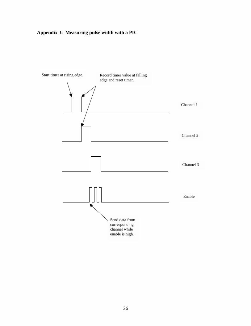
the I/O addresses, and sets the number of inputs or outputs. As described below, the three s-functions (vsbcrad, vsbc6ad, vsbcenc) at the left of the Simulink model each serve a function in data acquisition (from radio receiver or sensors), while the s-function block on the right (vsbcser) handles servo actuation. The purpose of the ‘vsbcrad’ driver, in conjunction with the PIC radio monitor, is to handle data acquisition from the radio receiver. It sets the eight lower bits of the digital I/O address to input and the eight upper bits to output. All eight lower bits serve as data lines from the PIC, while one of the upper bits is the data transfer enable line (the rest are unused). ‘Vsbcser’ uses the computer’s counter feature to create and send PWM signals to the servos. Two counter lines are used: one for the steering servo and the other for the brake/throttle servo. Given a desired pulse width value, the counter automatically outputs the pulse width-modulated (PWM) signal. Due to an unavoidable characteristic of the counter, the PWM signals must be inverted before passing on to the servos. On the sensor side, ‘vsbc6ad’ takes care of analog-to-digital conversion for the yaw rate and two accelerometer measurements through the analog lines. Lastly, the ‘vsbcenc’ driver works with the PIC pulse monitor to obtain wheel speed information. Similar to ‘vsbcrad,’ there are eight data lines and one data transfer enable line. Actual vehicle speed in meters per second is calculated from a formula involving the newest pulse count, the last pulse count (stored from the previous sampling period), number of teeth in the gear, drive ratio, tire diameter, and sampling rate. We chose to place this calculation in the Simulink model to ease future modification of parameter values. PIC microcontroller The wheel speed sensor and radio receiver signals must be monitored continuously to capture rising and falling edges; the only way for the computer to do this without taking up all of the computing time is to use interrupts. An alternative approach is to relegate the continuous tasks to a separate programmable devices and periodically seek updates from the devices. The PIC is an inexpensive, easy-to-use microcontroller especially suited for this type of low level task, and more importantly, it leaves the computer free to deal with the higher level operations. The computer retrieves the critical information—wheel speed pulse counts and radio PWM pulse width—from the PICs only when needed. A transfer is typically requested by sending a pulse over an enable line; the PIC responds with a single set of data over the data lines. In our application, there are multiple sets of data (three radio channels, and up to four wheel speed signals) and insufficient I/O ports to give each set its own data lines. As a solution, multiple pulses are sent through the enable line, with each subsequent pulse initiating data transfer for the next set over the same data lines. Appendix J describes how we use a PIC to measure pulse width of the three PWM receiver channels. The pulses occur every 17 milliseconds with a nominal duty cycle of 9 percent, or a pulse width of 1.5 millisecond. Full range of steering (also full brake to full throttle, auxiliary switch on to switch off) is 6 percent to 12 percent duty cycle (1.0 to 2.0 millisecond pulse width). The three PWM signals are not in phase, but staggered such

9

that when the pulse width of the first channel ends, the second channel’s pulse width begins—and the third channel follows at the end of the second. The PIC measures pulse width by waiting for a rising edge, starting the timer, waiting for the signal to return to low, and recording the timer value at that instant. The timer is then reset for the next pulse width. In order to match the timer frequency to the pulse width and to avoid overflowing the timer before reset, we apply a prescaler of 32 to the 10 MHz PIC operating speed. The timer value has a maximum length of eight bits (0 to 255 in base ten); with the prescaler, neutral position (steering centered, no throttle or brake applied) corresponds with 118 on the base ten scale, and full range goes from approximately 80 to 160. The wheel speed PIC employs a programming strategy similar to the radio receiver PIC except that each rising edge triggers a register to increment by one (see Appendix K). Although the wheel speed PIC was programmed with a four-sensor capacity, only one sensor is being used at the present time. The assembly language code written for the two PICs can be found in Appendix N. Single board access We have been using one of three methods to access the single board computer’s ‘c:’ drive (Disk On Chip) and to run executable files on the car. The first method is to hook up a monitor, keyboard, and mouse to the single board computer running on DOS. File transfer can be done by attaching a floppy disk drive. The other two methods, which are better suited for field testing, allow access via laptop computer. One method involves communication over a cable connecting the COM ports on the laptop and computer; a terminal window on the laptop provides the interface, and file transfer is by the Kermit program. We recently implemented wireless Ethernet communication and at the same time switched to the XPC target environment. VI. Applications Radio signal filter One of the problems we noticed when testing the RC car with the computer system is that when the car moves farther away from the transmitter, the computer begins to record increasingly noisy radio signals. This noise, which appears as wildly fluctuating spikes in the pulse width values, also occurs near strong sources of electromagnetic radiation such as power lines. Frequently the noise is of such magnitude that it cause the servos to twist beyond the normal range of motion. To prevent damage to the servo systems and, more critically, loss of vehicle control, we tried adding a radio signal filter block in the Simulink model. The filter is designed to eliminate those signals that reach beyond the normal servo operating range (approximately 80 to 160 pulse width units). Another annoying, but less dangerous noise problem occurs when the servos are in their neutral position or being commanded to hold a constant position. The discretization of

10

the radio signals by the computer causes the servos to jitter as they flip between two adjacent values closest to the commanded value. To maintain smooth servo action, the filter holds the previous value for the current time step if the new value is less than two units (or bit changes) away from the old value. Testing shows that the filter block, shown below, does not completely eliminate all noise problems, but at least it minimizes the erratic servo behavior that would otherwise occur.

1Out1

speed

scale to m/s

steeringthrottle

Servo Output

vsbcrad

Radio Intercept

f rom receiv er

Filter

vsbcenc

Encoder Input

emu

emu

emuvsbc6ad

Analog Input

Simulink model with filter: cartestf.mdl.

1

z

1

[ch1off,ch2off,ch3off]

|u|1from receiver

Filter sub-model.

Speed control Our first attempt at implementing a controller on the RC car test bed was to add a speed control system based on the wheel speed sensor output. The ability to hold the car at constant speed during handling maneuvers is necessary for analyzing certain aspects of vehicle behavior and drawing meaningful comparisons between sets of test data. Control is accomplished with simple proportional gain feedback. In addition to speed control, the Simulink model shown below contains a feature for performing ramp steer maneuvers using the auxiliary switch. Appendix C explains the speed control/ramp steer program in

11

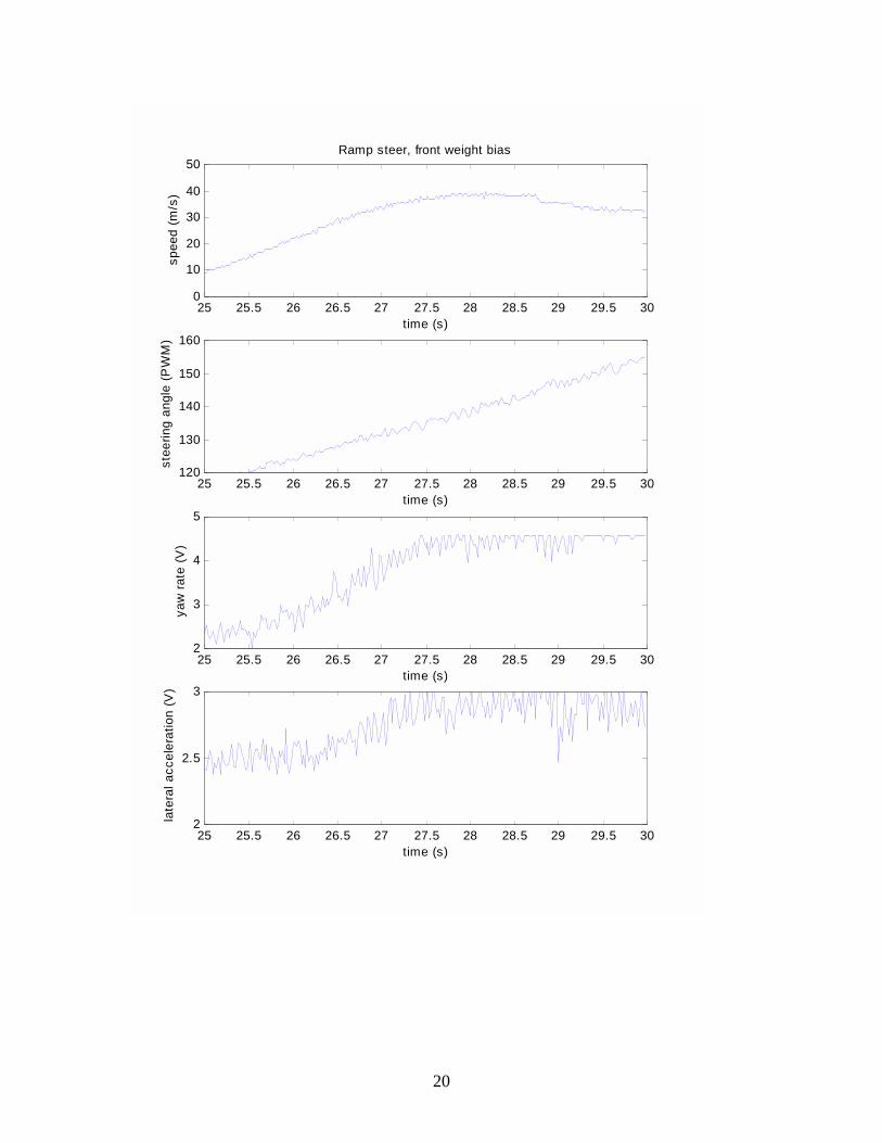
greater detail. A few selected results from a step steer and ramp steer test are shown in Appendix D.

1Out1

to steerinto throttle

to servos

analog input

encoder input

radio intercept

to steering

to throttle

accdes

controller

vsbcrad2

Radio Intercept

vsbcencs

Encoder Input

vsbc6ad

Analog Input

Simulink model: spdc.mdl.

3accdes

2to throttle

1to steering

???

switch sig

signal

y(n)=Cx(n)+Du(n)x(n+1)=Ax(n)+Bu(n)regulatorch2off

pw2spdkf rom receiv er

fi lter

cnts2spd

ffgain

m

0

3radio intercept

2encoder input

1analog input

Controller sub-model.

12

1sig

f(u)

gain selection

z

1

??? stsigk stsig2pwgain|u|

1switch

Ramp steer (switch signal) sub-model.

VII. Work in Progress Future vehicle dynamics and controls work will require knowledge of the various vehicle parameters. So far we have measured mass, yaw moment of inertia, center of gravity location, and steering ratio. This data is available in a separate report. We have recently made a number of improvements to the RC car test bed by switching to the more user-friendly XPC target environment and wireless Ethernet communication between computer and laptop. We have also enhanced operating safety by adding an independent, electronically-controlled engine kill switch that is directly activated via the auxiliary switch on the transmitter. These improvements will be detailed in a later report.

13

VIII. Acknowledgements Special thanks to: Samuel Chang, for developing the speed controller. Samuel Kim, for designing the computer enclosure box. The other members of the Dynamic Design Lab, Michael Prados, Matthew Schwall, Eric Rossetter, Santosh Heinrich, Jihan Ryu, and Robert Sheridan, who contributed their time, effort, and knowledge in building, testing, and debugging the RC car test bed, from the first one tenth-scale model to the current one quarter-scale configuration.

14

Appendix A: Single board computer setup procedure

1. Change jumper V10 to 1-2 position to accommodate Disk On Chip. 2. Install RAM and DOC. 3. Boot without floppy, go to ‘Setup.’ Setup menu can always be reached during

boot up by repeatedly pressing the ‘Delete’ key. 4. Enable DOC by setting ‘32 Pin Socket’ in Advanced Configuration to ‘DOC.’ 5. Select drive C to be in ‘Boot Order’ in Basic Configuration. 6. Boot with PC DOS, do not install. 7. Type ‘sys c:’ at the prompt. 8. Reboot with PC DOS, install. 9. Create ‘kermit’ directory on DOC and copy all Kermit files to the directory. 10. Edit ‘autoexec.bat’ file for Kermit. It should appear as follows:

@ECHO OFF PATH=C:\DOS;C:\KERMIT SET TEMP=C:\DOS C:\DOS\MOUSE.COM C:\DOS\DOSKEY.COM kermit.exe exit ctty com1

11. Create ‘rtwtest’ directory. Copy ‘dos4gw.exe’ to directory.

15

Appendix B: Code generation with Real-Time Workshop

1. Create an s-function block found under 'Simulink, Functions & Tables.’ 2. Double click on the block. 3. Enter the name of the s-function (ex. vsbenc) and its parameters (ex.

numChannels,sampTime). 4. Choose 'Mask s-function' under the 'Edit' menu. 5. Select 'Initialization' tab. 6. Enter parameter 'Prompt' (ex. Number of Channels) and corresponding 'Variable'

name (ex. numChannels). 7. Parameters can be changed later by choosing 'Edit Mask' under 'Edit' menu. 8. Create the rest of the Simulink model. 9. Set up simulation parameters, such as end time and time step, in 'RTW Options...'

under the 'Tools' menu. ‘Solver’ is discrete, fixed-step. Under ‘Real-Time Workshop…Code generation.,’ choose ‘drt.tlc’ (DOS) as the system target file. This choice requires that the Watcom C compiler be installed on the machine.

10. Run the associated MATLAB m-file (ex. carfile.m) to supply numerical values to any variables used in the model.

11. Compile the s-function code at the MATLAB command line (ex. mex vsbenc.c). Code must be re-compiled following any changes.

12. Build the simulation using 'RTW Build' under the 'Tools' menu. This function generates C code directly from the model and creates a DOS executable file (ex. cartest.exe) of the same name. Rebuild simulation to apply changes to s-functions or model.

16

Appendix C: RC Car Operating Procedures 1. Accessing the onboard computer You will be accessing the onboard computer via the laptop. First, connect the serial cable from the laptop to the communication port on the car. Double click on the ‘hypercar’ icon to open up a terminal window. Turn on main power to boot up the onboard computer (switch on the left side skirt of the car). After waiting about 30 seconds, a ‘c:\’ DOS prompt should appear in the terminal window. This is the ‘c:\’ drive of the onboard computer. 2. Transferring an executable file to the computer You only need to do this once or when you change the Simulink model. Run ‘kermit’ in the terminal window. Type ‘receive’ and choose ‘send file’ in the ‘File Transfer’ pull-down menu. Type in the DOS executable file name, ‘spdc.exe.’ Destination is the ‘c:\rtwtest’ directory. The transfer takes less than a minute. 3. Executing the ramp steer program Open the ‘c:\rtwtest’ directory. Type ‘spdc’ and press ‘return.’ The ramp steer program is now running and you are ready to begin performing the test. Make sure there is auxiliary power to the sensor and radio signal circuitry (switch on right side of box). You can now disconnect the serial cable from the car. 4. Turning on the servo motors First, turn on the handheld transmitter. Then, turn on power to the servo motors (black switch attached to the right side of box). You want to avoid turning on the servo motors when the transmitter is off or when the program is not running. Otherwise, irregular servo signals may cause the motors to twist beyond their normal range of motion. 5. Starting the engine Always make sure the brakes are applied before starting the engine. As an extra precaution, you may want to have someone hold the rear wheels off the ground or stand in front of the car to prevent it from running away. If the engine is cold, pump the fuel reservoir two or three times, close the choke, and pull the starter cord. To aid in starting, open the throttle slightly. Let the engine idle for about a minute, then open the choke fully. To start a warm engine, just pull the starter cord. To kill the engine, depress the red button on the engine cover.

17

6. Performing the ramp steer test The ramp steer program does two things: 1) it maintains the car at a steady speed when you hold the throttle controller at a constant position, and 2) it initiates a ramp steering input when you engage the auxiliary switch on the handheld controller. To perform the ramp steer test, accelerate the car to its maximum preset speed (throttle switch fully open). Hit the auxiliary switch to initiate the ramp steer. When the steering has reached full lock, move the auxiliary switch in the opposite direction to return the steering to the straight ahead position. Be prepared to apply the brakes in case anything goes wrong. The test program will run for a preset length of time, and the car will brake automatically when the program ends. 7. Adjusting the transmitter After running the program for the first time, you may wish to change the transmitter settings. To change to maximum throttle opening when the throttle lever is fully engaged, press the ‘mode’ button on the transmitter repeatedly until the display reads ‘th.atv.’ Press ‘+’ to increase or decrease the throttle opening. To switch the response direction of the throttle lever and steering wheel, press the ‘mode’ and ‘select’ buttons at the same time. Press ‘mode’ again to reach the steering (‘st’) display, then ‘+’ to switch direction to ‘reverse’ or ‘normal.’ Press ‘select’ to go to the throttle (‘th’) display. 8. Transferring test data to the laptop The sensor and radio signal data collected during the test is stored on the onboard computer in file ‘spdc.mat.’ To transfer the file to the laptop, reconnect the serial cable to the car. Run ‘kermit’ in the terminal window. Type ‘send spdc.mat’ and press ‘return.’ Choose ‘receive’ in the ‘File Transfer’ pull-down menu and click ‘OK.’ The file takes several minutes to download. Exit Kermit when the transfer is completed. You can now load the file in MATLAB to view the data. 9. Format of ‘spdc.mat’ The output file consists of a time vector ‘rt-tout’ and 12 columns of data, ‘rt_yout’:

1. yaw rate (V) 2. lateral acceleration (V) 3. longitudinal acceleration (V) 4. wheel speed (m/s) 5. wheel speed (m/s)—not connected 6. wheel speed (m/s)—not connected 7. wheel speed (m/s)—not connected 8. signal from steering controller (pulse width) 9. signal from throttle/brake controller (pulse width) 10. signal from auxiliary switch (pulse width)

18

11. signal to steering servo (pulse width) 12. signal to throttle/brake servo (pulse width)

Notes: ! Data column 11 does not indicate saturation of the ramp input (when steering

reaches limit). ! Yaw rate sensor saturates at 64 degrees per second. ! Sensor outputs are voltages and must be scaled to appropriate units.

19

Appendix D: Sample test data

18 18.5 19 19.5 20 20.5 21 21.5 22 22.5 230

10

20

30

40

50Step steer, front weight bias

time (s)

spee

d (m

/s)

18 18.5 19 19.5 20 20.5 21 21.5 22 22.5 23120

130

140

150

160

time (s)

stee

ring

angl

e (P

WM

)

18 18.5 19 19.5 20 20.5 21 21.5 22 22.5 232

3

4

5

time (s)

yaw

rate

(V)

18 18.5 19 19.5 20 20.5 21 21.5 22 22.5 232

2.5

3

time (s)

late

ral a

ccel

erat

ion

(V)

20

25 25.5 26 26.5 27 27.5 28 28.5 29 29.5 300

10

20

30

40

50Ramp steer, front weight bias

time (s)

spee

d (m

/s)

25 25.5 26 26.5 27 27.5 28 28.5 29 29.5 30120

130

140

150

160

time (s)

stee

ring

angl

e (P

WM

)

25 25.5 26 26.5 27 27.5 28 28.5 29 29.5 302

3

4

5

time (s)

yaw

rate

(V)

25 25.5 26 26.5 27 27.5 28 28.5 29 29.5 302

2.5

3

time (s)

late

ral a

ccel

erat

ion

(V)

21

Appendix E: Circuit diagram

22

Appendix F: Radio interface circuit board

40 PIN EXT DIG

POWER/GROUND

PIC

14 PIN T/C

INV

OSC

TO SERVOS

FROM RECEIVER

1 2 3

1

2

ST TH SW

ST

TH

23

Appendix G: I/O pinouts for radio interface board GND

GND GND GND GND

O5 I5O4I4

O3

9 7 5 3 1

10 8 6 4 2

Ribbon Cable

GND GND GND GND GND GND GND GND GND GND GND GND GND GND GND GND GND

D0 D1 D2 D3 D4 D5 D6 D7 D8 D9 D10 D11 D12 D13 D14 D15 +5V

2 4 6 8 10 12 14 16 18 20 22 24 26 28 30 32 34

1 3 5 7 9

11 13 15 17 19 21 23 25 27 29 31 33

Ribbon Cable

Timer/Counter I/O

External Digital I/O

24

HALL EFFECT

40 PIN DIG

GYRO POWER/GROUND

PIC

16 PIN AN

BUFF

OSC/R

RC FILTER

ACCEL

1

2

3

Appendix H: Sensor interface circuit board

25

Appendix I: I/O pinouts for sensor interface board

A0 GND A3 A4 GND A7 NC NC

A1 A2

GND A5 A6

GND GND GND

2 4 6 8 10 12 14 16

1 3 5 7 9

11 13 15

GND GND GND GND GND GND GND GND GND GND GND GND GND GND GND GND GND

Ribbon Cable

D0 D1 D2 D3 D4 D5 D6 D7 D8 D9 D10 D11 D12 D13 D14 D15 +5V

18 20 22 24 26 28 30 32 34 36 38 40 42 44 46 48 50

17 19 21 23 25 27 29 31 33 35 37 39 41 43 45 47 49

Ribbon Cable

Standard Analog I/O

Standard Digital I/O

26

Appendix J: Measuring pulse width with a PIC

Channel 1

Channel 2

Channel 3

Enable

Start timer at rising edge. Record timer value at falling edge and reset timer.

Send data from corresponding channel while enable is high.

27

Appendix K: Counting pulses with a PIC

Increment counter at each rising edge.

Sensor 1

Sensor 2

Sensor 3

Enable

Send data from corresponding channel while enable is high.

Sensor 4

28

Appendix L: Simulink m-file clear all % sampling period (s) Ts = 0.02 % simulation end time (s) Tf = 60 % servo output (pulse width units) brake = 85 % filter (pulse width units) ch1off = 118 ch2off = 118 ch3off = 118 ch1max = 38 ch2max = 38 ch3max = 38 % scale pulse counts to m/s tire_circ = 0.479 gear_teeth = 30 drive_ratio = 4.5 speed = tire_circ / (Ts*gear_teeth*drive_ratio)

29

Appendix M: Device Drivers /* * vsbcrad.c: Device Driver for External Digital I/O * for Radio Signal Interception * py 12/14/99 * py 3/5/00 revised * Based on sfuntmpl.c: C template for a level 2 S-function.

*/ #define S_FUNCTION_LEVEL 2 #define S_FUNCTION_NAME vsbcrad #include <stdlib.h> #include “simstruc.h” /*=========================================================================* * Number of S-function Parameters and macros to access from the SimStruct * *=========================================================================*/ #define NUM_PARAMS (2) #define NUM_CHANNELS_PARAM (ssGetSFcnParam(S,0)) #define SAMPLE_TIME_PARAM (ssGetSFcnParam(S,1)) /*==================================================* * Macros to access the S-function parameter values * *==================================================*/ #define NUM_CHANNELS ((uint_T) mxGetPr(NUM_CHANNELS_PARAM)[0]) #define AD_SAMPLE_TIME ((uint_T) mxGetPr(SAMPLE_TIME_PARAM)[0]) /*=======================================* * Addresses for Timer/Counter Registers * *=======================================*/ #define CONTROL (0x300) #define PARWLO (0x306) #define PARWHI (0x307) #define PARRLO (0x306) #define PARRHI (0x307) /*====================* * S-function methods * *====================*/ /* Function: mdlInitializeSizes =============================================== * Abstract: * The sizes information is used by Simulink to determine the S-function * block’s characteristics (number of inputs, outputs, states, etc.). */ static void mdlInitializeSizes(SimStruct *S) { ssSetNumSFcnParams(S, NUM_PARAMS); /* Number of expected parameters */ if (ssGetNumSFcnParams(S) != ssGetSFcnParamsCount(S)) { /* Return if number of expected != number of actual parameters */ return; } ssSetNumContStates(S, 0); ssSetNumDiscStates(S, 0); ssSetNumInputPorts(S, 0); ssSetNumOutputPorts(S, 1); ssSetOutputPortWidth(S, 0, NUM_CHANNELS); ssSetNumSampleTimes(S, 1); ssSetNumRWork(S, 0); ssSetNumIWork(S, 0); ssSetNumPWork(S, 0); ssSetNumModes(S, 0);

30

ssSetNumNonsampledZCs(S, 0); ssSetOptions(S, 0); } /* Function: mdlInitializeSampleTimes ========================================= * Abstract: * This function is used to specify the sample time(s) for your * S-function. You must register the same number of sample times as * specified in ssSetNumSampleTimes. */ static void mdlInitializeSampleTimes(SimStruct *S) { ssSetSampleTime(S, 0, AD_SAMPLE_TIME); ssSetOffsetTime(S, 0, 0.0); } /* Function: mdlOutputs ======================================================= * Abstract: * In this function, you compute the outputs of your S-function * block. Generally outputs are placed in the output vector, ssGetY(S). */ static void mdlOutputs(SimStruct *S, int_T tid) { real_T *Radio = ssGetOutputPortRealSignal(S,0); uint_T i,j; outp(CONTROL,0x80); for (i = 0; i < NUM_CHANNELS; i++) { outp(PARWHI,0x01); // set enable high and delay for PIC for (j = 0; j < 10000; j++) { } Radio[i] = inp(PARRLO); // get pulse width for channel i outp(PARWHI,0x00); // set enable low and delay for PIC for (j = 0; j < 10000; j++) { } } } /*=============================* * Required S-function trailer * *=============================*/ #ifdef MATLAB_MEX_FILE /* Is this file being compiled as a MEX-file? */ #include “simulink.c” /* MEX-file interface mechanism */ #else #include “cg_sfun.h” /* Code generation registration function */ #endif

31

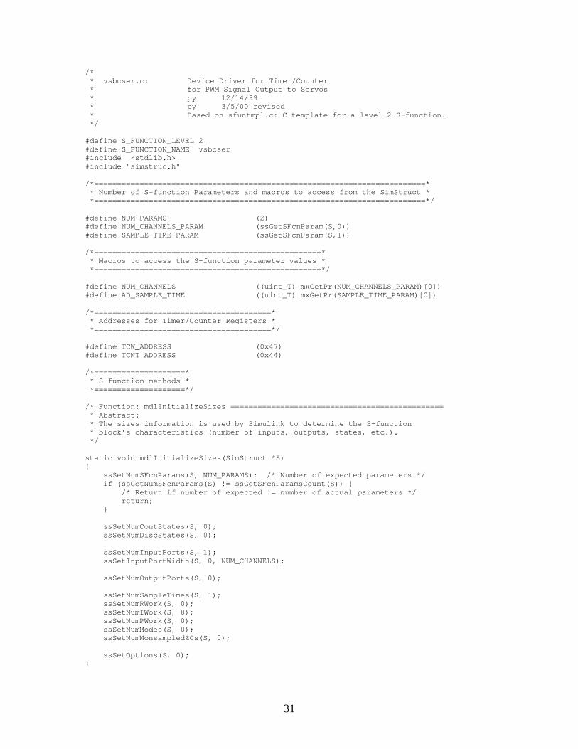
/* * vsbcser.c: Device Driver for Timer/Counter * for PWM Signal Output to Servos * py 12/14/99 * py 3/5/00 revised * Based on sfuntmpl.c: C template for a level 2 S-function. */ #define S_FUNCTION_LEVEL 2 #define S_FUNCTION_NAME vsbcser #include <stdlib.h> #include "simstruc.h" /*=========================================================================* * Number of S-function Parameters and macros to access from the SimStruct * *=========================================================================*/ #define NUM_PARAMS (2) #define NUM_CHANNELS_PARAM (ssGetSFcnParam(S,0)) #define SAMPLE_TIME_PARAM (ssGetSFcnParam(S,1)) /*==================================================* * Macros to access the S-function parameter values * *==================================================*/ #define NUM_CHANNELS ((uint_T) mxGetPr(NUM_CHANNELS_PARAM)[0]) #define AD_SAMPLE_TIME ((uint_T) mxGetPr(SAMPLE_TIME_PARAM)[0]) /*=======================================* * Addresses for Timer/Counter Registers * *=======================================*/ #define TCW_ADDRESS (0x47) #define TCNT_ADDRESS (0x44) /*====================* * S-function methods * *====================*/ /* Function: mdlInitializeSizes =============================================== * Abstract: * The sizes information is used by Simulink to determine the S-function * block’s characteristics (number of inputs, outputs, states, etc.). */ static void mdlInitializeSizes(SimStruct *S) { ssSetNumSFcnParams(S, NUM_PARAMS); /* Number of expected parameters */ if (ssGetNumSFcnParams(S) != ssGetSFcnParamsCount(S)) { /* Return if number of expected != number of actual parameters */ return; } ssSetNumContStates(S, 0); ssSetNumDiscStates(S, 0); ssSetNumInputPorts(S, 1); ssSetInputPortWidth(S, 0, NUM_CHANNELS); ssSetNumOutputPorts(S, 0); ssSetNumSampleTimes(S, 1); ssSetNumRWork(S, 0); ssSetNumIWork(S, 0); ssSetNumPWork(S, 0); ssSetNumModes(S, 0); ssSetNumNonsampledZCs(S, 0); ssSetOptions(S, 0); }

32

/* Function: mdlInitializeSampleTimes ========================================= * Abstract: * This function is used to specify the sample time(s) for your * S-function. You must register the same number of sample times as * specified in ssSetNumSampleTimes. */ static void mdlInitializeSampleTimes(SimStruct *S) { ssSetSampleTime(S, 0, AD_SAMPLE_TIME); ssSetOffsetTime(S, 0, 0.0); } /* Function: mdlOutputs ======================================================= Abstract: In this function, you compute the outputs of your S-function block. Generally outputs are placed in the output vector, ssGetY(S). */ static void mdlOutputs(SimStruct *S, int_T tid) { InputRealPtrsType NewSignal = ssGetInputPortRealSignalPtrs(S,0); uint_T i,j; real_T Servo[2],Time; int_T Counts,LSB,MSB; for (i = 0; i < 2; i++) { Servo[i] = *NewSignal[i]; } for (j = 0; j < 2; j++) {

Time = (Servo[j]*4*32)/10; // calculate duration of pulse (sec*10^6) Counts = 6 * Time; // number of counts while low LSB = Counts % 256; // least significant byte of counts MSB = Counts / 256; // most significant byte of counts outp(TCW_ADDRESS,(0x30+64*j)); // write control word to register outp(TCNT_ADDRESS+j,LSB); // write counts to counter register outp(TCNT_ADDRESS+j,MSB); } } /*=============================* * Required S-function trailer * *=============================*/ #ifdef MATLAB_MEX_FILE /* Is this file being compiled as a MEX-file? */ #include “simulink.c” /* MEX-file interface mechanism */ #else #include “cg_sfun.h” /* Code generation registration function */ #endif

33

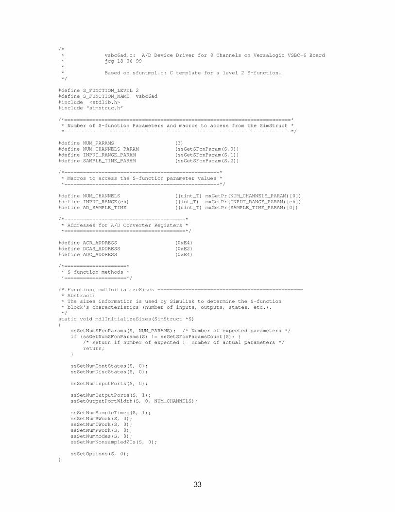
/* * vsbc6ad.c: A/D Device Driver for 8 Channels on VersaLogic VSBC-6 Board * jcg 18-06-99 * * Based on sfuntmpl.c: C template for a level 2 S-function. */ #define S_FUNCTION_LEVEL 2 #define S_FUNCTION_NAME vsbc6ad #include <stdlib.h> #include “simstruc.h” /*=========================================================================* * Number of S-function Parameters and macros to access from the SimStruct * *=========================================================================*/ #define NUM_PARAMS (3) #define NUM_CHANNELS_PARAM (ssGetSFcnParam(S,0)) #define INPUT_RANGE_PARAM (ssGetSFcnParam(S,1)) #define SAMPLE_TIME_PARAM (ssGetSFcnParam(S,2)) /*==================================================* * Macros to access the S-function parameter values * *==================================================*/ #define NUM_CHANNELS ((uint_T) mxGetPr(NUM_CHANNELS_PARAM)[0]) #define INPUT_RANGE(ch) ((int_T) mxGetPr(INPUT_RANGE_PARAM)[ch]) #define AD_SAMPLE_TIME ((uint_T) mxGetPr(SAMPLE_TIME_PARAM)[0]) /*=======================================* * Addresses for A/D Converter Registers * *=======================================*/ #define ACR_ADDRESS (0xE4) #define DCAS_ADDRESS (0xE2) #define ADC_ADDRESS (0xE4) /*====================* * S-function methods * *====================*/ /* Function: mdlInitializeSizes =============================================== * Abstract: * The sizes information is used by Simulink to determine the S-function * block’s characteristics (number of inputs, outputs, states, etc.). */ static void mdlInitializeSizes(SimStruct *S) { ssSetNumSFcnParams(S, NUM_PARAMS); /* Number of expected parameters */ if (ssGetNumSFcnParams(S) != ssGetSFcnParamsCount(S)) { /* Return if number of expected != number of actual parameters */ return; } ssSetNumContStates(S, 0); ssSetNumDiscStates(S, 0); ssSetNumInputPorts(S, 0); ssSetNumOutputPorts(S, 1); ssSetOutputPortWidth(S, 0, NUM_CHANNELS); ssSetNumSampleTimes(S, 1); ssSetNumRWork(S, 0); ssSetNumIWork(S, 0); ssSetNumPWork(S, 0); ssSetNumModes(S, 0); ssSetNumNonsampledZCs(S, 0); ssSetOptions(S, 0); }

34

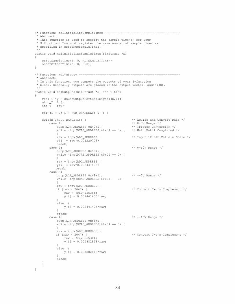
/* Function: mdlInitializeSampleTimes ========================================= * Abstract: * This function is used to specify the sample time(s) for your * S-function. You must register the same number of sample times as * specified in ssSetNumSampleTimes. */ static void mdlInitializeSampleTimes(SimStruct *S) { ssSetSampleTime(S, 0, AD_SAMPLE_TIME); ssSetOffsetTime(S, 0, 0.0); } /* Function: mdlOutputs ======================================================= * Abstract: * In this function, you compute the outputs of your S-function * block. Generally outputs are placed in the output vector, ssGetY(S). */ static void mdlOutputs(SimStruct *S, int_T tid) { real_T *y = ssGetOutputPortRealSignal(S,0); uint_T i,j; int_T raw; for (i = 0; i < NUM_CHANNELS; i++) { switch(INPUT_RANGE(i)) { /* Aquire and Convert Data */ case 1: /* 0-5V Range */ outp(ACR_ADDRESS,0x40+i); /* Trigger Conversion */ while((inp(DCAS_ADDRESS)&0x04)== 0) { /* Wait Until Completed */ } raw = inpw(ADC_ADDRESS); /* Input 12 bit Value & Scale */ y[i] = raw*0.001220703; break; case 2: /* 0-10V Range */ outp(ACR_ADDRESS,0x50+i); while((inp(DCAS_ADDRESS)&0x04)== 0) { } raw = inpw(ADC_ADDRESS); y[i] = raw*0.002441406; break; case 3: outp(ACR_ADDRESS,0x48+i); /* +-5V Range */ while((inp(DCAS_ADDRESS)&0x04)== 0) { } raw = inpw(ADC_ADDRESS); if (raw > 2047) { /* Convert Two’s Complement */ raw = (raw-65536); y[i] = 0.002441406*raw; } else { y[i] = 0.002441406*raw; } break; case 4: /* +-10V Range */ outp(ACR_ADDRESS,0x58+i); while((inp(DCAS_ADDRESS)&0x04)== 0) { } raw = inpw(ADC_ADDRESS); if (raw > 2047) { /* Convert Two’s Complement */ raw = (raw-65536); y[i] = 0.004882813*raw; } else { y[i] = 0.004882813*raw; } break; } } }

35

/*=============================* * Required S-function trailer * *=============================*/ #ifdef MATLAB_MEX_FILE /* Is this file being compiled as a MEX-file? */ #include “simulink.c” /* MEX-file interface mechanism */ #else #include “cg_sfun.h” /* Code generation registration function */ #endif

36

/* * vsbcenc.c: Digital Input/Output Device Driver for 16 Channels on * VersaLogic VSBC-6 Board * py 7-8-99 * sc 3-4-00 revised * Based on sfuntmpl.c: C template for a level 2 S-function. */ #define S_FUNCTION_LEVEL 2 #define S_FUNCTION_NAME vsbcenc #include <stdlib.h> #include “simstruc.h” /*=========================================================================* * Number of S-function Parameters and macros to access from the SimStruct * *=========================================================================*/ #define NUM_PARAMS (2) #define NUM_CHANNELS_PARAM (ssGetSFcnParam(S,0)) #define SAMPLE_TIME_PARAM (ssGetSFcnParam(S,1)) /*==================================================* * Macros to access the S-function parameter values * *==================================================*/ #define NUM_CHANNELS ((uint_T) mxGetPr(NUM_CHANNELS_PARAM)[0]) #define AD_SAMPLE_TIME ((uint_T) mxGetPr(SAMPLE_TIME_PARAM)[0]) /*=======================================* * Addresses for A/D Converter Registers * *=======================================*/ #define DCAS_ADDRESS (0xE2) #define DIOLO_ADDRESS (0xE6) #define DIOHI_ADDRESS (0xE7) /*====================* * S-function methods * *====================*/ /* Function: mdlInitializeSizes =============================================== * Abstract: * The sizes information is used by Simulink to determine the S-function * block’s characteristics (number of inputs, outputs, states, etc.). */ static void mdlInitializeSizes(SimStruct *S) { ssSetNumSFcnParams(S, NUM_PARAMS); /* Number of expected parameters */ if (ssGetNumSFcnParams(S) != ssGetSFcnParamsCount(S)) { /* Return if number of expected != number of actual parameters */ return; } ssSetNumContStates(S, 0); ssSetNumDiscStates(S, 0); ssSetNumInputPorts(S, 0); ssSetNumOutputPorts(S, 1); ssSetOutputPortWidth(S, 0, NUM_CHANNELS); ssSetNumSampleTimes(S, 1); ssSetNumRWork(S, 0); ssSetNumIWork(S, NUM_CHANNELS); ssSetNumPWork(S, 0); ssSetNumModes(S, 0); ssSetNumNonsampledZCs(S, 0); ssSetOptions(S, 0); }

37

/* Function: mdlInitializeSampleTimes ========================================= * Abstract: * This function is used to specify the sample time(s) for your * S-function. You must register the same number of sample times as * specified in ssSetNumSampleTimes. */ static void mdlInitializeSampleTimes(SimStruct *S) { ssSetSampleTime(S, 0, AD_SAMPLE_TIME); ssSetOffsetTime(S, 0, 0.0); } #define MDL_INITIALIZE_CONDITIONS /* Change to #undef to remove function */ #if defined(MDL_INITIALIZE_CONDITIONS) /* Function: mdlInitializeConditions ======================================== * Abstract: * In this function, you should initialize the continuous and discrete * states for your S-function block. The initial states are placed * in the state vector, ssGetContStates(S) or ssGetRealDiscStates(S). * You can also perform any other initialization activities that your * S-function may require. Note, this routine will be called at the * start of simulation and if it is present in an enabled subsystem * configured to reset states, it will be call when the enabled subsystem * restarts execution to reset the states. */ static void mdlInitializeConditions(SimStruct *S) { int_T k; for (k = 0; k < NUM_CHANNELS; k++) { ssSetIWorkValue(S,k,0); } } #endif /* MDL_INITIALIZE_CONDITIONS */ /* Function: mdlOutputs ======================================================= * Abstract: * In this function, you compute the outputs of your S-function * block. Generally outputs are placed in the output vector, ssGetY(S). */ static void mdlOutputs(SimStruct *S, int_T tid) { real_T *Speed = ssGetOutputPortRealSignal(S,0); int_T i; outp(DCAS_ADDRESS,0x02); // initialize D0-D7 as input, D8-D15 as output for (i = 0; i < NUM_CHANNELS; i++) { int_T Counts, NewCount, j; outp(DIOHI_ADDRESS,0x01); // set enable high and delay for PIC for (j = 0; j < 10000; j++) { } NewCount = inp(DIOLO_ADDRESS); // update current count for Encoder I outp(DIOHI_ADDRESS,0x00); // set enable low and delay for PIC for (j = 0; j < 10000; j++) { } if (ssGetIWorkValue(S,i) > NewCount) // if counter has rolled over { Counts = (256 – ssGetIWorkValue(S,i)) + NewCount; } else Counts = NewCount – ssGetIWorkValue(S,i);

38

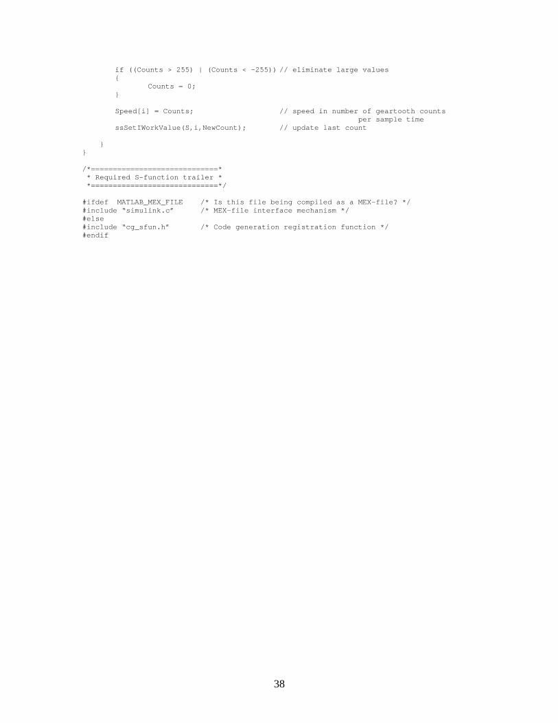
if ((Counts > 255) | (Counts < -255)) // eliminate large values { Counts = 0; } Speed[i] = Counts; // speed in number of geartooth counts per sample time ssSetIWorkValue(S,i,NewCount); // update last count } } /*=============================* * Required S-function trailer * *=============================*/ #ifdef MATLAB_MEX_FILE /* Is this file being compiled as a MEX-file? */ #include “simulink.c” /* MEX-file interface mechanism */ #else #include “cg_sfun.h” /* Code generation registration function */ #endif

39

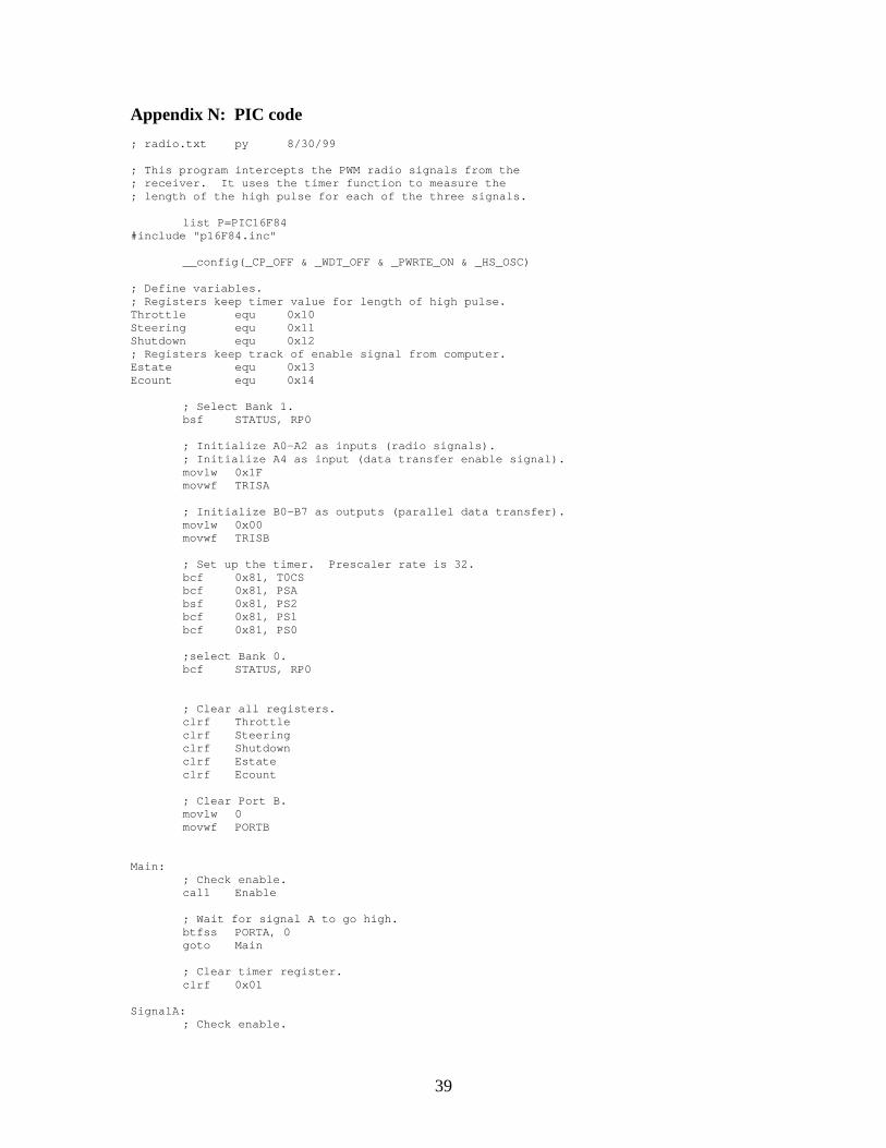
Appendix N: PIC code ; radio.txt py 8/30/99 ; This program intercepts the PWM radio signals from the ; receiver. It uses the timer function to measure the ; length of the high pulse for each of the three signals. list P=PIC16F84 #include "p16F84.inc" __config(_CP_OFF & _WDT_OFF & _PWRTE_ON & _HS_OSC) ; Define variables. ; Registers keep timer value for length of high pulse. Throttle equ 0x10 Steering equ 0x11 Shutdown equ 0x12 ; Registers keep track of enable signal from computer. Estate equ 0x13 Ecount equ 0x14 ; Select Bank 1. bsf STATUS, RP0 ; Initialize A0-A2 as inputs (radio signals). ; Initialize A4 as input (data transfer enable signal). movlw 0x1F movwf TRISA ; Initialize B0-B7 as outputs (parallel data transfer). movlw 0x00 movwf TRISB ; Set up the timer. Prescaler rate is 32. bcf 0x81, T0CS bcf 0x81, PSA bsf 0x81, PS2 bcf 0x81, PS1 bcf 0x81, PS0 ;select Bank 0. bcf STATUS, RP0 ; Clear all registers. clrf Throttle clrf Steering clrf Shutdown clrf Estate clrf Ecount ; Clear Port B. movlw 0 movwf PORTB Main: ; Check enable. call Enable ; Wait for signal A to go high. btfss PORTA, 0 goto Main ; Clear timer register. clrf 0x01 SignalA: ; Check enable.

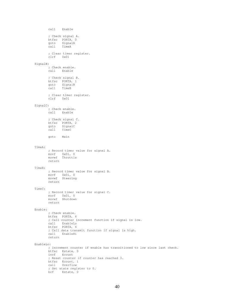
40

call Enable ; Check signal A. btfsc PORTA, 0 goto SignalA call TimeA ; Clear timer register. clrf 0x01 SignalB: ; Check enable. call Enable ; Check signal B. btfsc PORTA, 1 goto SignalB call TimeB ; Clear timer register. clrf 0x01 SignalC: ; Check enable. call Enable ; Check signal C. btfsc PORTA, 2 goto SignalC call TimeC goto Main TimeA: ; Record timer value for signal A. movf 0x01, 0 movwf Throttle return TimeB: ; Record timer value for signal B. movf 0x01, 0 movwf Steering return TimeC: ; Record timer value for signal C. movf 0x01, 0 movwf Shutdown return Enable: ; Check enable. btfss PORTA, 4 ; Call counter increment function if signal is low. call EnableLo btfsc PORTA, 4 ; Call data transmit function if signal is high. call EnableHi return EnableLo: ; Increment counter if enable has transitioned to low since last check. btfsc Estate, 0 incf Ecount ; Reset counter if counter has reached 3. btfsc Ecount, 1 call Overflow ; Set state register to 0. bcf Estate, 0

41

return Overflow: btfsc Ecount, 0 clrf Ecount return EnableHi: ; Check value of enable counter and send data from corresponding register. btfss Ecount, 1 call AorB btfsc Ecount, 1 call SendC ; Set state register to 1. bsf Estate, 0 return AorB: btfss Ecount, 0 call SendA btfsc Ecount, 0 call SendB return SendA: movf Throttle, 0 movwf PORTB return SendB: movf Steering, 0 movwf PORTB return SendC: movf Shutdown, 0 movwf PORTB return end

42

; encoder.txt py 8/30/99 ; This program multiplexes the square wave outputs from up to ; four encoder-type wheel speed sensors. It keeps count of ; the square pulses for each sensor signal. list P=PIC16F84 #include "p16F84.inc" __config (_CP_OFF & _WDT_OFF & _PWRTE_ON & _HS_OSC) ; Define variables. ; Registers keep current count of each encoder signal. CounterA equ 0x10 CounterB equ 0x11 CounterC equ 0x12 CounterD equ 0x13 ; Register keeps track of which encoder data has been sent. CounterE equ 0x14 ; Registers indicate whether the signals are high or low. StateA equ 0x15 StateB equ 0x16 StateC equ 0x17 StateD equ 0x18 StateE equ 0x19 ; Select Bank 1. bsf STATUS, RP0 ; Initialize A0-A3 as inputs (encoder signals). ; Initialize A4 as input (data transfer enable signal). movlw 0x1F movwf TRISA ; Initialize B0-B7 as outputs (parallel data transfer). movlw 0x00 movwf TRISB ; Select Bank 0. bcf STATUS, RP0 Start: ; Clear all registers. clrf CounterA clrf CounterB clrf CounterC clrf CounterD clrf CounterE clrf StateA clrf StateB clrf StateC clrf StateD clrf StateE ; Clear Port B. movlw 0 movwf PORTB ; Wait for enable to go high. btfss PORTA, 4 goto Start Main: ; Check each encoder signal. ; Set state register to 0 if signal is low. ; Call counter increment function if signal is high. ; Check encoder A. btfss PORTA, 0 bcf StateA, 0 btfsc PORTA, 0

43

call EncoderA ; Check encoder B. btfss PORTA, 1 bcf StateB, 0 btfsc PORTA, 1 call EncoderB ; Check encoder C. btfss PORTA, 2 bcf StateC, 0 btfsc PORTA, 2 call EncoderC ; Check encoder D. btfss PORTA, 3 bcf StateD, 0 btfsc PORTA, 3 call EncoderD ; Check enable. btfss PORTA, 4 ; Call counter increment function if signal is low. call EnableLo btfsc PORTA, 4 ; Call data transmit function if signal is high. call EnableHi goto Main EnableLo: ; Increment enable counter if enable signal has transitioned to low since last check. btfsc StateE, 0 incf CounterE ; Reset counter if counter has reached 4. btfsc CounterE, 2 clrf CounterE ; Set state register to 0. bcf StateE, 0 return EnableHi: ; check value of enable counter and send data from corresponding register btfss CounterE, 1 call AorB btfsc CounterE, 1 call CorD ; Set state register to 1. bsf StateE, 0 return AorB: btfss CounterE, 0 call SendA btfsc CounterE, 0 call SendB return CorD: btfss CounterE, 0 call SendC btfsc CounterE, 0 call SendD return SendA: movf CounterA, 0 movwf PORTB return

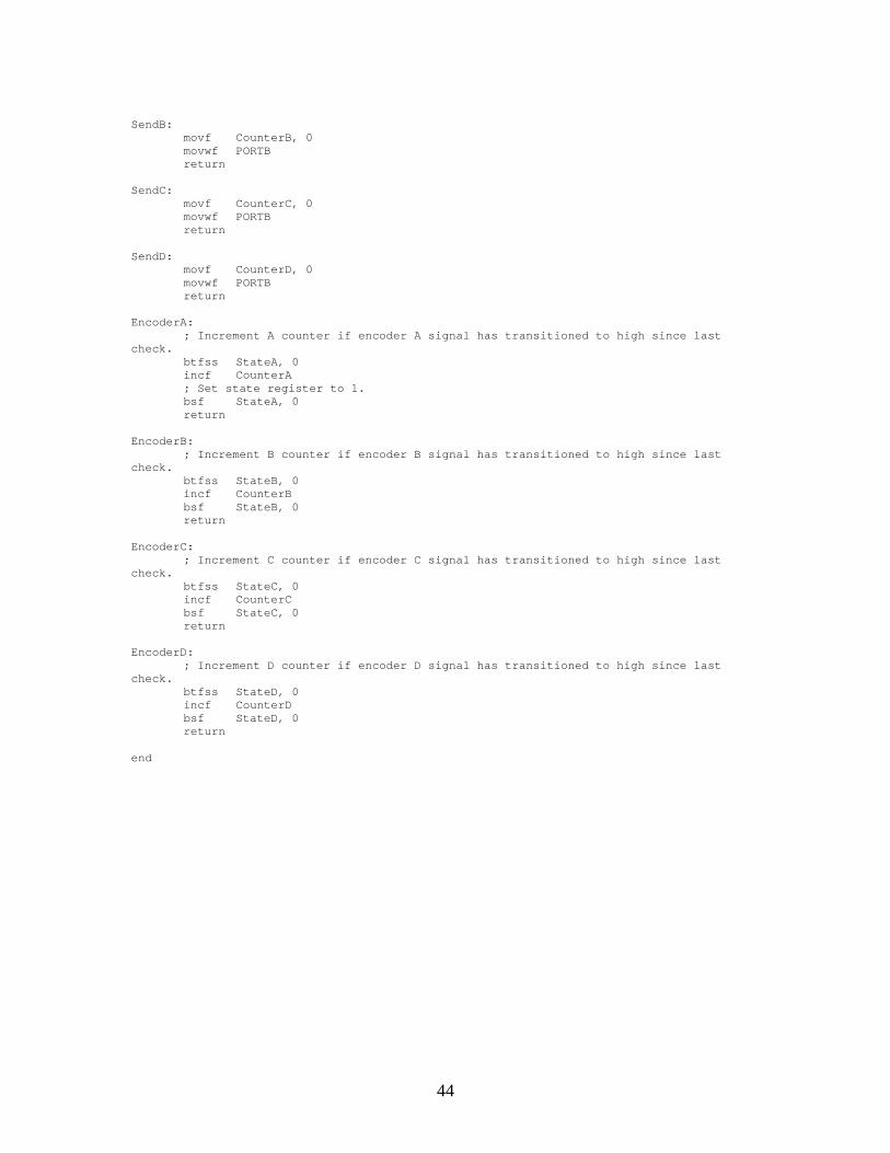
44

SendB: movf CounterB, 0 movwf PORTB return SendC: movf CounterC, 0 movwf PORTB return SendD: movf CounterD, 0 movwf PORTB return EncoderA: ; Increment A counter if encoder A signal has transitioned to high since last check. btfss StateA, 0 incf CounterA ; Set state register to 1. bsf StateA, 0 return EncoderB: ; Increment B counter if encoder B signal has transitioned to high since last check. btfss StateB, 0 incf CounterB bsf StateB, 0 return EncoderC: ; Increment C counter if encoder C signal has transitioned to high since last check. btfss StateC, 0 incf CounterC bsf StateC, 0 return EncoderD: ; Increment D counter if encoder D signal has transitioned to high since last check. btfss StateD, 0 incf CounterD bsf StateD, 0 return end

45

Appendix O: List of suppliers Suppliers of mechanical hardware New Era Models (www.neweramodels.com)

Partially assembled one quarter-scale RC car with necessary hardware including Futaba servo motors and radio controller/receiver system

Zenoah (www.zenoah.com)

One cylinder two stroke gasoline engine

San Antonio Hobby Shop (San Antonio Shopping Center, Mountain View) In-line fuel filter, plastic antenna holder, 7.2V RC car battery

Home Depot

Aluminum side skirts, exhaust pipe Orchard Supply Hardware (2555 Charleston Road, Mountain View)

Chain saw spark plug, miscellaneous hardware Palo Alto Hardware

Miscellaneous hardware Suppliers of electrical hardware Jameco (1355 Shoreway Road, Belmont)

30 W DC-DC converter, 12V rechargeable lead acid battery, .100” IDC DIP flat cable plugs, wire wrap IC sockets

Digikey (www.digikey.com)

.062” white Molex connectors, 0.100” black Molex locking connectors, white Molex “toy car” battery connector, SOIC to DIP adapter (for accelerometer mounting), electronic supplies

Halted Specialties Company (3500 Ryder Street, Santa Clara)

Miscellaneous connectors, PC boards, electronic supplies Radio Shack

SPDT switches, electronic supplies Suppliers of computer hardware and sensors Versalogic Corporation (www.versalogic.com)

VSBC-6 single board computer and accessories

46

Microchip (www.microchip.com) 16F84 PIC microcontrollers, PICSTART Plus PIC programmer Analog Devices (www.analogdevices.com)

ADXL202 dual axis accelerometer Systron Donner (www.systron.com)

AQRS automotive angular rate sensor Newark Electronics (www.newark.com)

Honeywell hall effect gear tooth sensor for wheel speed measurement Motion Industries, Inc. (160 Constitution Drive, Menlo Park)

Steel spur gear (12 diametral pitch, 30 teeth, 14.5 degree pressure angle) for wheel speed sensor