Radiation Shielding and Reactor Criticality

Fall 2013

By Yaohang Li, Ph.D.

Review• Last Class

– Test of Randomness

– Chi-Square Test

– KS Test

• This Class– Monte Carlo Application in Nuclear Physics

• Radiation Shielding

• Reactor Criticality

• Simulation of Collisions

– Self-avoiding random walk

– Assignment #5

• Markov Chain Monte Carlo

Monte Carlo Method in Nuclear Physics

• Flux of uncharged particles through a medium– Uncharged particles

• paths between collisions are straight lines

• do not influence one another– independence

– allow us to take the behavior of a relatively small sample of particles to represent the whole

– Randomness

• derive the Monte Carlo methods directly from the physical processes

Problem Definition• Particle (Photon or Neutron)

– energy E– instantaneously at the point r– traveling in the direction of the unit vector

• Traveling of the Particle– At each point of its straight path it has a chance of colliding with an atom

of the medium• No collision with an atom of the medium

– continue to travel in the same direction with same energy E

• A probability of cs that the particle will collide with an atom of the medium

s: a particle traverses a small length of its straight line– c: cross section

» depends on the nature of surrounding medium» energy E

Cross Section

• Determining c

– The medium remains homogeneous within each of a small number of distinct regions

• over each region, c is a constant

c change abruptly on passing from one region to the next

– Example

• Uranium rods immersed in water c a function of E in the rods

c another function of E in the water

Collision• Collision Probability

– cdf of the distance that the particle travels before collision• Fc(s) = 1 – exp(- c s)

• Three situations of collision– Absorption

• the particle is absorbed into the medium– Scatter

• the particle leaves the point of collision in a new direction with a new energy with probability (Ei)

– fission (only arises when the original particle is a neutron)• several other neutrons, known as secondary neutrons, leaves the point

of collision with various energies and directions

• Probability of the three situations– Governed by the physical law– Known distribution from Monte Carlo point of view

Shielding and Criticality Problems

• The Shielding Problem– When a thick shield of absorbing material is exposed to -

radiation (photons), of specified energy and angle of incidence, what is the intensity and energy-distribution of the radiation that penetrates the shield?

• The Criticality Problem– When a pulse of neutron is injected into a reactor assembly,

will it cause a multiplying chain reaction or will it be absorbed, and in particular, what is the size of the assembly at which the reaction is just able to sustain itself?

Elementary Approach• Elementary Approach

– Exact realization of the physical model

• Not very efficient

– Tracking of simulated particles from collision to collision

• Starting with a particle (E, , r)

• Generate a number s with the exponential distribution– Fc(s) = 1 – exp(- c s)

• If the straight-line path from r to (r+s) does not intersect any boundary (between regions)

– the particle has a collision

• Otherwise– proceed as far as the first boundary

– if this is the outer boundary, the particle escapes from the system

• Repeat the procedure

Improvements of the Elementary Approach

• Problem– There may be too many or too few particles– Consider a reactor containing a very fissile component

• Every neutron entering this region may give rise to a very large number coming out

– Give us more tracks than we have time to follow• Solution

– “Russian Roulette”• Pick out one of the particles

– discard it with probability p– otherwise allow this particle to continue but multiply its weight (initially unity) by

(1-p)-1

• The number of particles is reduced to manageable size– “Splitting”

• To increase the sample sizes– a particle of weight w may be replaced by any number k of identical particles of

weights w1, …, wk» w1+…+wk=w

Special Methods for the Shielding Problem

• Outstanding feature of the shielding problem– The proportion of photons that penetrate the shield is very small, say one in

106.

– To estimate an accuracy of 10% require the number of 108 paths.

• Hit or miss

• Quite inefficient

• Solution– Semi-analytic method

– Allows the same random paths to be used for shields of other thickness

– Simplification

• Only think about three coordinates– Energy E

– Angle between the direction of motion and the normal to the stab

– Distance z from the incident face of the slab

The Semi-Analytic Method (I)•A random history

– for a particle which undergoes a suitably large number n of scatterings in the medium

•The semi-analytic method– Pi()

• The probability that a particle has a history hi and also crosses the plane z= between its ith and (i+1)th scatterings

– Abbreviation (α is the absorption probability)

• ci=cosi; i=c(Ei); i=[1-(Ei)]c(Ei)

– P0()=exp(- i/c0)

• the probability that the particle passes through z= before suffering any scatterings

– Pi+1()

• A particle crosses z= between its (i+1)th and (i+2)th scatterings

n

nn

EEEhh

,...,,

,...,,

10

10

The Semi-Analytic Method (II)

•The semi-analytic method– the (i+1)th scattering occurred on some a plane z= ’ where 0<’< .

– Compound event

• i: immediately prior to the (i+1)th scattering the particle crossed z= ’– P(i)=Pi(’)

• ii: the particle suffered the (i+1)th scattering between the planes z= ’ and z= ’+d’

– P(ii)= i d’/|ci|

• iii: after scattering, the particle now travels with energy E i+1 in direction i+1

– P(iii)= exp(- i+1(- ’) /ci+1)

– Then

– The probability of penetrating the shield is

0

111 ||

'}/)'(exp{)'()(

i

iiiii c

dcPP

))((0

ii tPE

Probability of Penetration

• Replace with• Approximate unbiased estimator of penetration

probability• N = 25, 12, 9, 6 is efficient for shields of water, iron, tin,

and lead

))((0

ii tPE ))((

0

N

ii tPE

Neutron Transport• Transmission of Neutrons

– Bulk matter

• Plate– thickness t

– infinite in the x and y directions

– z axis is normal to the plate

– Neutron at any point in the plate

• Capture with probability pc

– Proportional to capture cross section

• Scatter with probability ps

– Proportional to scattering cross section

Scattering

•Scattering– polar angle – azimuthal angle

• we are not interested in how far the neutron moves in x or y direction, the value of is irrelevant

X

Z

v v'

Solid Angle

• 2D– measured by unit angles

(radians)

– full circle subtends 2

• 3D– measured by unit solid angles

(steradians)

– full sphere subtends 4

Probability of Scattering

•Scattering equally in all directions– probability p(,)dd=d/4

•Definition of the Solid Angle

– then d = sindd– we can get p(,) = sin/4

•Probability density for and

S

dd sin

2

0

sin2

1),()( dpp

0 2

1),()( dpp

Non-uniform Random Sample Generation Revisit

•Probability Density p(x)

•Then

– r is a uniform random number

•Inverse Function Method– use r to represent x

1)( dxxp

x

rdxxpxP ')'()(

Randomizing the Angles

=2r is uniformly distributed between 0 and 2

– Then we can get cos = 1-2r

– cos is uniformly distributed between -1 and +1

0

sin2

1xdxr

Path Length

•Path length– distance traveled between subsequent scattering events

– obtained from the exponential probability density function

– l=-lnr is the mean free path

• or the cross section constant c

/)/1()( lelp

Neutron Transport Algorithm (1)

• Input parameters– thickness of the plate t

– capture probability pc

– scattering probability ps

– mean free path

• Initial value z=0

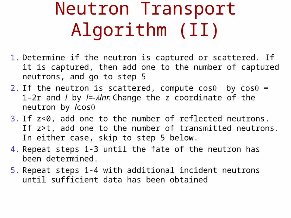
Neutron Transport Algorithm (II)

1. Determine if the neutron is captured or scattered. If it is captured, then add one to the number of captured neutrons, and go to step 5

2. If the neutron is scattered, compute cos by cos = 1-2r and l by l=-lnr. Change the z coordinate of the neutron by lcos

3. If z<0, add one to the number of reflected neutrons. If z>t, add one to the number of transmitted neutrons. In either case, skip to step 5 below.

4. Repeat steps 1-3 until the fate of the neutron has been determined.

5. Repeat steps 1-4 with additional incident neutrons until sufficient data has been obtained

An Improved Method

• Instead of Considering A Neutron– Consider a set of neutrons

– ps portion of neutrons are scattered

• All scattered neutrons will move to a new direction

– pc portion of neutrons are captured

• A better convergence rate

Properties of Polymers

• Hydrophobic– The attraction between monomers is stronger than their

attraction to the molecules of the surrounding solvent, e.g., water

• Hydrophilic– The attraction between monomers is weaker than their

attraction to the molecules of the surrounding solvent, e.g., water

• Non Self-intersect– No two monomers can occupy the same place

• excluded volume

Solvent

• Low Temperature (or in a poor solvent)– The attractive interactions between monomers pull the polymer

into a dense ball-like configuration

– globule

• High Temperature (or in good solvent)– The interactions are mediated by the solvent molecules

– Typical configurations are open coils

• Phase Transition– Coil-Globule transition

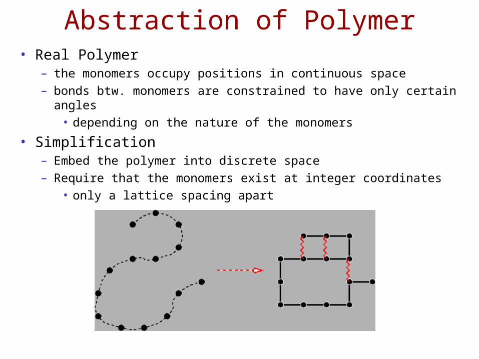
Abstraction of Polymer• Real Polymer

– the monomers occupy positions in continuous space

– bonds btw. monomers are constrained to have only certain angles

• depending on the nature of the monomers

• Simplification– Embed the polymer into discrete space

– Require that the monomers exist at integer coordinates

• only a lattice spacing apart

Radius• Average size of a polymer containing n monomers• Radius of gyration

– average distance of a monomer from the polymer’s center of mass– <Rn

2> ~ Anv

• v is the critical exponent– in the swollen phase: v 0.588– in the collapse phase: v=1/3

• A is unknown– use linear regression

Early Solution

• Goal– Estimate <Rn

2>

• Method– Generate unrestricted random walks

– Accept if no interception

– Not accept if interception

• Problem– Not efficient

Self-avoiding Random Walk

• Self-avoiding Random Walk– Walk on 2D or 3D lattice

– Explore the geometric properties of linear polymers in good solvent

– Constraint random walk (don’t allow to go backward)

– Introduced by Orr

• Analysis of Self-avoiding Random Walks– At first glance, the model is far too simple

– Phenomenon of universality

• Many quantities are not dependent on the specific details of the system

• They are determined only by its universality class

• All systems in the same universality class share the same dominant asymptotic behavior

A Picture is Worth a Thousand Words

3D Walk2D Walk

Self-avoiding Random Walk

Algorithm

#include <iostream.h>#include <stdlib.h>#include <math.h>

void do_walk (int maxstep, int& nstep, double& rsquared ){ const int MAXSTEP=20; int map[ MAXSTEP*2][MAXSTEP*2]={0};

// start point int completed=0; int x = MAXSTEP; int y = MAXSTEP; int npoint = 1; map[x][y] = npoint; do { int xnew=x; int ynew=y;

switch ( (int)(4 *(double)rand()/(RAND_MAX+1.0)) ) { case 0: xnew-= 1; break; case 1: xnew+= 1; break; case 2: ynew-= 1; break; case 3: ynew+= 1; break; }if ( map[xnew][ynew] == 0 ){ npoint++; map[xnew][ynew] = npoint; x = xnew; y = ynew; if ( npoint == maxstep+1 )completed=1; } else if ( map[xnew][ynew] != npoint-1 ) { completed=1; } } while ( !completed );

// Print window centred on map for ( int i=5; i<2*MAXSTEP-5; i++ ){ for ( int j=5; j < 2*MAXSTEP-5; j++ ){ cout.width(3); cout << map[i][j]; } cout << endl; } nstep = npoint-1; rsquared = pow( x-MAXSTEP,2.0) + pow( y-MAXSTEP, 2.0 );}

int main(){ int maxstep=20,nstep; double rsquared; srand(987654321); for (int i=1; i<10; i++ ){ do_walk(maxstep,nstep,rsquared); cout << endl << "Nsteps: " <<nstep << " Rsquared: " <<rsquared<<endl; } return 0;}

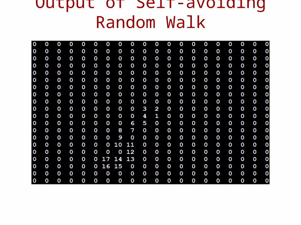
Output of Self-avoiding Random Walk

Biased Random Walk

• Problems of self-avoiding random walk– Have to reject many terminated walks in order to have

unbiased statistics– Unlikely to produce long polymer– Inefficiency

• Biased Random Walk– Basic Idea

• Instead of abandoning a walk when an illegal step is attempted, we go back and pick one of the possible legal steps

• Enable a walk to make a full distance

Biased Random Walk Algorithm

• Weight Factor W(N)– Initially = 1– 3 possibilities

• No further steps are possible, we have reached a dead end

– Abandon this walk

• All steps, other than going directly backwards are possible

– proceed as normal, set W(N) = W(N-1)

• Only m steps are possible– Randomly choose one of the possible steps– set W(N)=m/3*W(N)

Output of Biased Random Walk

Summary• Nuclear Simulation

– Radiation Shielding– Reactor Criticality– Particle Assumption

• Cross Section• Collision

– Elementary Method– Improvements for the Elementary Method

• Russian Roulette• Splitting

– Special methods for the shielding problem• Semi-Analytic Method

– Neutron Transport Problem– Nonuniform Distribution Samples

Summary• Long Polymer Molecule• Self-avoiding Random Walk• Biased Random Walk

What I want you to do?

• Review Slides• Review basic probability/statistics concepts• Work on your Assignment 5