RADIATION FROM CAVITY-BACKED FRACTAL APERTURE ANTENNAS · PDF fileRADIATION FROM CAVITY-BACKED...

Progress In Electromagnetics Research C, Vol. 11, 155–170, 2009

RADIATION FROM CAVITY-BACKED FRACTALAPERTURE ANTENNAS

B. Ghosh, S. N. Sinha, and M. V. Kartikeyan

Department of Electronics and Computer EngineeringIndian Institute of Technology RoorkeeRoorkee 247667, India

Abstract—This paper investigates the properties of probe fed cavity-backed fractal aperture antennas. The problem is formulated usingthe finite element-boundary integral (FE-BI) method in which the fieldinside the cavity is formulated using the finite element method, andthe mesh is truncated at cavity aperture surface using the boundaryintegral method. Several dual-band cavity-backed fractal apertureantennas based on Sierpinski gasket, Sierpinski carpet, plus shapefractal and Minkowski fractal are investigated. The numerical resultsobtained from the FE-BI code have been validated with simulationson HFSS.

1. INTRODUCTION

Slot antennas form an important class of antennas which are preferredin applications where low-profile, flush-mounted, and conformalantennas are required. One shortcoming of slot antennas is theirbi-directional radiation characteristic which is alleviated by using ashallow cavity on one side of the slot. The performance of severalcavity-backed aperture antennas has been investigated in the past [1–4]. With the recent trends in the design of compact communicationsystems, a demand has arisen for antennas which can be operatedin multiple frequency bands. This has led to the use of fractalgeometries whose self-similarity property has been exploited in thedesign of a number of multi-band printed antennas. Recently, somefractal printed slot antennas have also been investigated using Kochfractal [5], circular fractal slot [6], and Sierpinski curves [7]. In thispaper, we investigate the radiation properties of some typical fractalslot antennas backed by a cavity.

Corresponding author: B. Ghosh ([email protected]).

156 Ghosh, Sinha, and Kartikeyan

The finite element-boundary integral (FE-BI) method has beenused to analyze the problem, since it is an efficient and versatilenumerical technique for the analysis of cavity-backed apertureantennas [8]. The technique employs the finite element method tocompute the electromagnetic field inside the cavity and the cavityvolume mesh is terminated at the aperture surface using boundaryintegral method [9]. The method generates a partly sparse and partlyfilled matrix which can be efficiently stored and solved. In the absenceof suitable fabrication facilities, simulation on HFSS has been used tovalidate the results obtained from FE-BI analysis.

The article is organized as follows: A general formulationof radiation from cavity-backed aperture antennas using the finiteelement-boundary integral method is presented in Section 2. InSection 3, numerical results of different cavity-backed fractal apertureantennas are presented. Section 4 summarizes the results.

2. FORMULATION OF THE PROBLEM

A typical coaxial probe-fed cavity-backed aperture antenna is shownin Fig. 1, where the apertures can be of arbitrary shape and number.The antenna is fed by a coaxial probe of inner radius ρ1 and outerradius ρ2 and is located at (xc, yc). The problem is formulated usingthe FE-BI method using tetrahedral elements for cavity discretization.The open region above the cavity top surface is truncated usingboundary integral (BI) method and the aperture surface at the bottomof the cavity is formulated using eigenfunction expansion method. Bycombining these three methods, the entire problem can be transformedinto a linear system.

Infinite

ground plane

Apertures

(Sap)

Rectangular

cavity

Input

Aperture

surface

(Sinp)

x

y

z

Z=z1

Coaxial Line

c c

Figure 1. Geometry of a coaxial probe-fed cavity backed apertureantenna.

Progress In Electromagnetics Research C, Vol. 11, 2009 157

For a linear, isotropic and source free region, the electric fieldsatisfies the vector wave equation given by

∇×(

1µr∇× E

)− k2

0εrE = 0 (1)

where µr and εr are, respectively, the permeability and permittivity ofthe medium inside the cavity.

Multiplying (1) scalarly by a testing function T and integratingover the volume of the cavity, we get

∫∫∫

VT · ∇ ×

(1µr∇× E

)dv − k2

oεr

∫∫∫

VT · Edv = 0 (2)

where V denotes the volume of the cavity.Using vector identities, the above expression can be written as∫∫∫

V

1µr

(∇×T) · (∇×E

)dv−k2

0εr

∫∫∫

VT · Edv=jωµ0©

∫∫

S(T×n) · Hds

(3)where n is the unit outward normal to cavity surface S.

The tangential component of the electric field is zero on theperfectly conducting walls of the cavity, except on the aperturesurfaces. Thus, the surface integral on the right hand side of (3) isnon zero only over the aperture surfaces (Sap) on the infinite groundplane and on the input aperture surface (Sinp) on the cavity bottom.Therefore, (3) can be rewritten as,

∫∫∫

V

1µr

(∇× T ) · (∇× E)dv − k20εr

∫∫∫

VT · E dv

−jωµ0

∫∫

Sap

(T × n) · Hapds = jωµ0

∫∫

Sinp

(T × n) · Hinpds (4)

where, Hap and Hinp denote the magnetic fields on the aperturesurfaces Sap and Sinp, respectively.

Thus, the problem can be divided into three parts. The firstpart involves the computation of volume integrals inside the cavityvolume. The second and third parts involve the evaluation of surfaceintegrals over the apertures on the top surface of the cavity and theinput aperture surface, respectively. The cavity is first discretized intosmall tetrahedral elements and over each tetrahedral element, vectoredge basis functions [10] are defined. The surface integral over theaperture surface on the top surface of the cavity is calculated using theequivalence principle and the magnetic field in the open space region iscalculated by considering an equivalent magnetic surface current 2M ,where M = E× z, radiating in free space. The surface integral over the


input surface at the bottom of cavity is computed by expanding theelectric field as the sum of incident and reflected fields. The procedureis same as that described in [11]. The combination of these threeintegrals can be expressed is matrix form as

A(k)e(k) = b(k) (5)

where b(k) is the excitation vector, e(k) denotes the coefficient vectorand A(k) is a partly sparse and partly dense matrix which is acombination of three matrices and may be written as

A(k) = A1(k) + A2(k) + A3(k) (6)

with

A1(k) =∫∫∫

V

1µr

(∇× T ) · (∇× E)dv − k20εr

∫∫∫

VT · Edv (7)

A2(k) = jk0Z0

∫∫

Sap

Ts · Hap(2M)ds (8)

A3(k) =jk0

√εrc

2π ln(

ρ2

ρ1

)∫∫

Sinp

(T · ρ

ρ

)ds

∫∫

Sinp

(E · ρ

ρ

)ds

(9)

b(k) =2jk0

√εrc√

2π ln(

ρ2

ρ1

)∫∫

Sinp

T ·(

ρ

ρ

)ds (10)

where εrc is the permittivity of material inside coaxial line.Once the matrix equation (5) is solved for the unknown

coefficients, the field over the aperture surface can be calculated. Theinput reflection coefficient at the incident plane (z1 = 0) is then givenby [11]

Γ =1√

2π ln(

ρ2

ρ1

)∫∫

Sinp

E · ρ

ρds− 1 (11)

The magnetic field in the far-field region can be calculated as

H(r, θ, ϕ) = −jk0

η0

e−jk0r

2πr

∫∫

Sap

(θθ + ϕϕ) · Mejk0 sin θ(x cos ϕ+y sin ϕ)dxdy

(12)

3. NUMERICAL RESULTS

Based on the formulation presented here, a MATLAB code has beendeveloped to analyze the performance of cavity-backed fractal aperture


antennas. Several fractal aperture antennas have been investigated andthe results are presented in the following subsections. For the apertureantennas considered here, the dimension of the cavity is taken to be15 cm×15 cm×0.4 cm and the cavity is assumed to be fed by a coaxialprobe of 50 Ω characteristic impedance.

3.1. Sierpinski Carpet Fractal Aperture

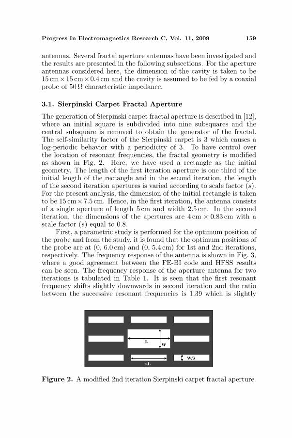
The generation of Sierpinski carpet fractal aperture is described in [12],where an initial square is subdivided into nine subsquares and thecentral subsquare is removed to obtain the generator of the fractal.The self-similarity factor of the Sierpinski carpet is 3 which causes alog-periodic behavior with a periodicity of 3. To have control overthe location of resonant frequencies, the fractal geometry is modifiedas shown in Fig. 2. Here, we have used a rectangle as the initialgeometry. The length of the first iteration aperture is one third of theinitial length of the rectangle and in the second iteration, the lengthof the second iteration apertures is varied according to scale factor (s).For the present analysis, the dimension of the initial rectangle is takento be 15 cm×7.5 cm. Hence, in the first iteration, the antenna consistsof a single aperture of length 5 cm and width 2.5 cm. In the seconditeration, the dimensions of the apertures are 4 cm × 0.83 cm with ascale factor (s) equal to 0.8.

First, a parametric study is performed for the optimum position ofthe probe and from the study, it is found that the optimum positions ofthe probe are at (0, 6.0 cm) and (0, 5.4 cm) for 1st and 2nd iterations,respectively. The frequency response of the antenna is shown in Fig. 3,where a good agreement between the FE-BI code and HFSS resultscan be seen. The frequency response of the aperture antenna for twoiterations is tabulated in Table 1. It is seen that the first resonantfrequency shifts slightly downwards in second iteration and the ratiobetween the successive resonant frequencies is 1.39 which is slightly

LW

s.L

W/3

Figure 2. A modified 2nd iteration Sierpinski carpet fractal aperture.


1.5 1.75 2 2.25 2.5 2.75 3 -20

-15

-10

-5

0

-25

Frequency (GHz)

Ret

urn

Loss

(d

B)

FE-BI

HFSS

(a) 1st Iteration

1.5 1.75 2 2.25 2.5 2.75 3 -30

-25

-20

-15

-10

-5

0

Frequency (GHz)

Ret

urn

Loss

(d

B)

FE-BI

HFSS

(b) 2nd Iteration

Figure 3. Return loss of modified Sierpinski carpet fractal apertureantenna with s = 0.8.

Table 1. Frequency response of modified Sierpinski carpet fractalaperture antenna.

Parameters Iteration 1 Iteration 2fr1 fr1 fr2

ResonantFreq. (GHz) 1.94 1.87 2.60

VSWR 1.25 1.09 1.32Bandwidth (%) 1.55 1.98 2.50

Table 2. Frequency response of modified Sierpinski carpet fractalaperture antenna for different scale factors.

Scale Factor Resonant Frequencies Ratio Bandwidth (%)(s) fr1 fr2 fr2/fr1 BW1 BW2

0.7 1.89 2.74 1.45 1.85 1.830.8 1.87 2.60 1.39 1.98 2.500.9 1.82 2.36 1.30 2.31 2.58

greater than the theoretical ratio of 1.25. The ratio between thesuccessive resonant frequencies can be controlled by changing the scalefactor (s). Two more fractal structures with different scale factors wereanalyzed. The variation of return loss of the antenna for different scalefactors is shown in Fig. 4 and the results are summarized in Table 2.

The optimum probe location for the two antennas with s = 0.7and s = 0.9 are (0, 5.7 cm) and (0, 5.0 cm), respectively. It is evidentthat while the first resonant frequency is relatively insensitive to the


1.5 1.75 2 2.25 2.5 2.75 3 -25

-20

-15

-10

-5

0

Frequency (GHz)

Ret

urn

Loss

(d

B)

s=0.7

s=0.8

s=0.9

Figure 4. Return loss of modified Sierpinski carpet fractal apertureantenna for different scale factors.

-40

-30

-20

-10

0

10

0

30

60

90

120

150

180

210

240

270

300

330

-40

-30

-20

-10

0

10

No

rm

ali

zed

Ra

dia

ted

Po

wer (

dB

)

(a) 1st Resonance

-40

-30

-20

-10

0

10

0

30

60

90

120

150

180

210

240

270

300

330

-40

-30

-20

-10

0

10

No

rm

ali

zed

Ra

dia

ted

Po

wer (

dB

)

(b) 2nd Resonance

=0

=90φφ

o

o =0

=90φ

φo

o

Figure 5. Normalized radiation pattern of modified Sierpinski carpetfractal aperture antenna with s = 0.8.

variation in scale factor and is primarily dependent on the size of initialrectangle; the second resonant frequency can be suitably located byselecting an appropriate scale factor. The frequency ratios are greaterthan the theoretical value which is a characteristic of the pre-fractalgeometries for lower order iterations. Also, the ratios between thesuccessive resonant frequencies depend on the position of slot relativeto the center of the cavity and the location of resonant frequencies canbe fine tuned by varying the spacing between the apertures.

The normalized radiation pattern of a 2nd iteration modifiedSierpinski carpet aperture in the two principal planes is shown in Fig. 5for s = 0.8. At the second resonant frequency (2.6GHz), the cavity isexcited in TM120 mode which has a field pattern such that the seconditeration apertures are excited in opposite phase, causing a null toappear along z -axis.


3.2. Self-affine Sierpinski Gasket Dipole Apertures

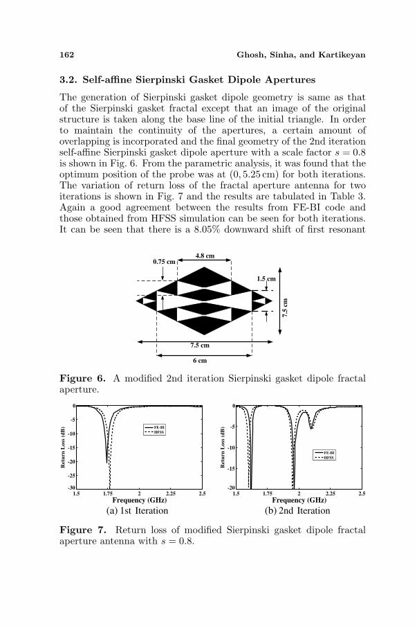
The generation of Sierpinski gasket dipole geometry is same as thatof the Sierpinski gasket fractal except that an image of the originalstructure is taken along the base line of the initial triangle. In orderto maintain the continuity of the apertures, a certain amount ofoverlapping is incorporated and the final geometry of the 2nd iterationself-affine Sierpinski gasket dipole aperture with a scale factor s = 0.8is shown in Fig. 6. From the parametric analysis, it was found that theoptimum position of the probe was at (0, 5.25 cm) for both iterations.The variation of return loss of the fractal aperture antenna for twoiterations is shown in Fig. 7 and the results are tabulated in Table 3.Again a good agreement between the results from FE-BI code andthose obtained from HFSS simulation can be seen for both iterations.It can be seen that there is a 8.05% downward shift of first resonant

7.5 cm

7.5

cm

6 cm

4.8 cm0.75 cm

1.5 cm

Figure 6. A modified 2nd iteration Sierpinski gasket dipole fractalaperture.

1.5 1.75 2 2.25 2.5 -30

-25

-20

-15

-10

-5

0

Frequency (GHz)

Retu

rn

Loss

(d

B) FE-BI

HFSS

(a) 1st Iteration

1.5 1.75 2 2.25 2.5 -20

-15

-10

-5

0

Frequency (GHz)

Retu

rn

Loss

(d

B)

FE-BI

HFSS

(b) 2nd Iteration

Figure 7. Return loss of modified Sierpinski gasket dipole fractalaperture antenna with s = 0.8.


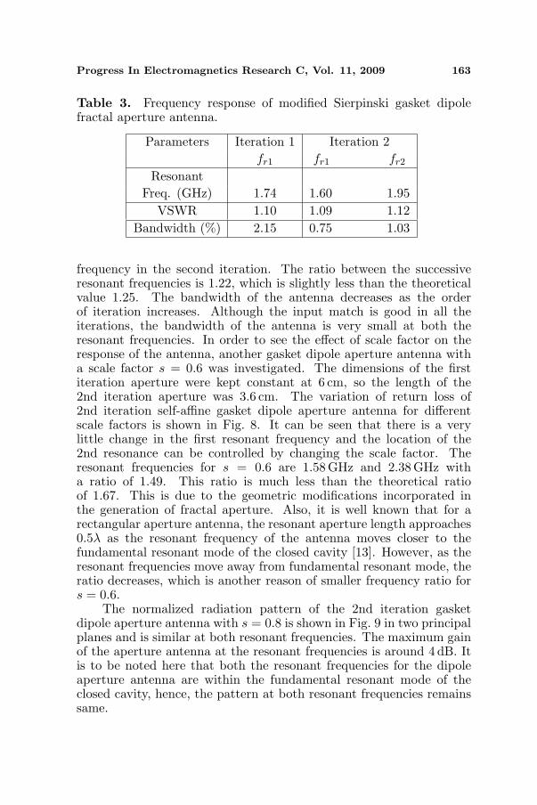
Table 3. Frequency response of modified Sierpinski gasket dipolefractal aperture antenna.

Parameters Iteration 1 Iteration 2fr1 fr1 fr2

ResonantFreq. (GHz) 1.74 1.60 1.95

VSWR 1.10 1.09 1.12Bandwidth (%) 2.15 0.75 1.03

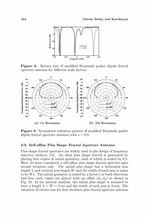
frequency in the second iteration. The ratio between the successiveresonant frequencies is 1.22, which is slightly less than the theoreticalvalue 1.25. The bandwidth of the antenna decreases as the orderof iteration increases. Although the input match is good in all theiterations, the bandwidth of the antenna is very small at both theresonant frequencies. In order to see the effect of scale factor on theresponse of the antenna, another gasket dipole aperture antenna witha scale factor s = 0.6 was investigated. The dimensions of the firstiteration aperture were kept constant at 6 cm, so the length of the2nd iteration aperture was 3.6 cm. The variation of return loss of2nd iteration self-affine gasket dipole aperture antenna for differentscale factors is shown in Fig. 8. It can be seen that there is a verylittle change in the first resonant frequency and the location of the2nd resonance can be controlled by changing the scale factor. Theresonant frequencies for s = 0.6 are 1.58 GHz and 2.38 GHz witha ratio of 1.49. This ratio is much less than the theoretical ratioof 1.67. This is due to the geometric modifications incorporated inthe generation of fractal aperture. Also, it is well known that for arectangular aperture antenna, the resonant aperture length approaches0.5λ as the resonant frequency of the antenna moves closer to thefundamental resonant mode of the closed cavity [13]. However, as theresonant frequencies move away from fundamental resonant mode, theratio decreases, which is another reason of smaller frequency ratio fors = 0.6.

The normalized radiation pattern of the 2nd iteration gasketdipole aperture antenna with s = 0.8 is shown in Fig. 9 in two principalplanes and is similar at both resonant frequencies. The maximum gainof the aperture antenna at the resonant frequencies is around 4 dB. Itis to be noted here that both the resonant frequencies for the dipoleaperture antenna are within the fundamental resonant mode of theclosed cavity, hence, the pattern at both resonant frequencies remainssame.


1.5 1.75 2 2.25 2.5 -20

-15

-10

-5

0

Frequency (GHz)

Ret

urn

Loss

(d

B)

s=0.8

s=0.6

Figure 8. Return loss of modified Sierpinski gasket dipole fractalaperture antenna for different scale factors.

-50

-40

-30

-20

-10

0

10

0

30

60

90

120

150

180

210

240

270

300

330

-50

-40

-30

-20

-10

0

10

No

rm

ali

zed

Ra

dia

ted

Po

wer (

dB

)

(a) 1st Resonance

-50

-40

-30

-20

-10

0

10

0

30

60

90

120

150

180

210

240

270

300

330

-50

-40

-30

-20

-10

0

10

No

rm

ali

zed

Ra

dia

ted

Po

wer (

dB

)

(b) 2nd Resonance

=0

=90φφ

o

o=0

=90φφ

o

o

Figure 9. Normalized radiation pattern of modified Sierpinski gasketdipole fractal aperture antenna with s = 0.8.

3.3. Self-affine Plus Shape Fractal Aperture Antenna

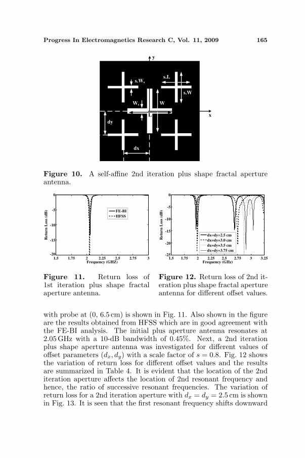
Plus shape fractal apertures are widely used in the design of frequencyselective surfaces [14]. An ideal plus shape fractal is generated byplacing four copies of initial geometry, each of which is scaled by 0.5.Here, we have considered a self-affine plus shape fractal aperture uptosecond iteration only. The initial plus shape has a horizontal armlength L and vertical arm length W and the width of each arm is takento be Ws. The initial geometry is scaled by a factor s in both directionsand four such copies are placed with an offset (dx, dy) as shown inFig. 10. In the present analysis, the initial plus shape is assumed tohave a length L = W = 5 cm and the width of each arm is 2 mm. Thevariation of return loss for first iteration plus fractal aperture antenna


L

WWs

s.L

s.W

s.Ws

x

y

dy

dx

Figure 10. A self-affine 2nd iteration plus shape fractal apertureantenna.

1.5 1.75 2 2.25 2.5 2.75 3 -20

-15

-10

-5

0

Frequency (GHZ)

Ret

urn

Loss

(d

B) FE-BI

HFSS

Figure 11. Return loss of1st iteration plus shape fractalaperture antenna.

1.5 1.75 2 2.25 2.5 2.75 3 3.25 -25

-20

-15

-10

-5

0

Frequency (GHz)

Ret

urn

Loss

(d

B)

dx=dy=2.5 cm

dx=dy=3.0 cm

dx=dy=3.5 cm

dx=dy=3.75 cm

Figure 12. Return loss of 2nd it-eration plus shape fractal apertureantenna for different offset values.

with probe at (0, 6.5 cm) is shown in Fig. 11. Also shown in the figureare the results obtained from HFSS which are in good agreement withthe FE-BI analysis. The initial plus aperture antenna resonates at2.05GHz with a 10-dB bandwidth of 0.45%. Next, a 2nd iterationplus shape aperture antenna was investigated for different values ofoffset parameters (dx, dy) with a scale factor of s = 0.8. Fig. 12 showsthe variation of return loss for different offset values and the resultsare summarized in Table 4. It is evident that the location of the 2nditeration aperture affects the location of 2nd resonant frequency andhence, the ratio of successive resonant frequencies. The variation ofreturn loss for a 2nd iteration aperture with dx = dy = 2.5 cm is shownin Fig. 13. It is seen that the first resonant frequency shifts downward


Table 4. Frequency response of 2nd iteration plus shape fractalaperture antenna for different offset values.

Offset xc yc Resonant Frequencies Ratio(dx = dy) (cm) (cm) f1 (GHz) f2 (GHz) f2/f1

2.50 0 6.6 1.97 2.69 1.373.00 0 6.4 1.99 2.75 1.383.50 0 6.4 2.00 2.87 1.443.75 0 6.25 2.00 2.91 1.46

1.5 1.75 2 2.25 2.5 2.75 3 -20

-15

-10

-5

0

Frequency (GHZ)

Ret

urn

Loss

(d

B)

FE-BI

HFSS

Figure 13. Return loss of2nd iteration plus shape fractalaperture antenna with dx = dy =2.5 cm and s = 0.8.

1.5 1.75 2 2.25 2.5 2.75 3 -20

-15

-10

-5

0

Frequency (GHZ)

Ret

urn

Loss

(d

B)

s=0.7

s=0.8

s=0.9

Figure 14. Return loss of 2nditeration plus shape fractal aper-ture for different scale factors.

and the ratio between the successive resonant frequencies is 1.36 ascompared to the theoretical value 1.25. Two more plus shape fractalapertures with scale factors s = 0.7 and s = 0.9 were investigatedand the results are shown in Fig. 14. The value of offset was keptat 2.5 cm. It is seen that the ratio between the successive resonantfrequencies are 1.425, 1.37 and 1.31 for s = 0.7, s = 0.8 and s = 0.9,respectively. Thus, the antenna resonant frequency can be controlledby changing the scale factor, which can be fine tuned with differentoffset values.

The radiation pattern of the 2nd iteration plus shape fractalaperture antenna is shown in Fig. 15. The pattern shows a similarbehavior as that of carpet antenna which shows a null along z-axis.

3.4. Minkowski Fractal Aperture Antenna

Minkowski fractal geometries are widely used in the miniaturizationof antenna and frequency selective surface design. Here, we haveconsidered a second iteration Minkowski aperture antenna. The


-50

-40

-30

-20

-10

0

10

0

30

60

90

120

150

180

210

240

270

300

330

-50

-40

-30

-20

-10

0

10

No

rm

ali

zed

Ra

dia

ted

Po

wer (

dB

)

(a) 1st Resonance

-50

-40

-30

-20

-10

0

10

0

30

60

90

120

150

180

210

240

270

300

330

-50

-40

-30

-20

-10

0

10

No

rm

ali

zed

Ra

dia

ted

Po

wer (

dB

)

(b) 2nd Resonance

=0

=90φφ

o

o =0

=90φφ

o

o

Figure 15. Normalized radiation pattern of self affine 2nd iterationplus shape fractal aperture antenna with s = 0.8.

dimension of the initial square is taken to be 3 cm × 3 cm and a10 cm× 10 cm× 0.4 cm cavity is used. The geometry of the Minkowskiaperture is shown in Fig. 16. From the parametric analysis, it wasfound that the optimum probe locations are (0, 4.25 cm), (0, 3.80 cm)and (0, 3.60 cm) for three iterations, respectively. The frequencyresponse of the Minkowski fractal aperture for different iterations ofthe fractal geometry is shown in Fig. 17. It is found that the resonantfrequency of the antenna decreases by 12.66% as the order of iterationincreases from 0th to 2nd iteration. The ratio of the square aperturelength to the resonant wavelength is 0.31. Generally, it is foundthat the antenna bandwidth decreases with the miniaturization ofthe antenna structure. However, in this case, the antenna bandwidthincreases as the order of iteration increases and the impedance matchfor all the iterations is very good.

The normalized power patterns of 2nd iteration Minkowskiaperture antenna at the resonant frequency are shown in Fig. 18.Although not shown in the figure, the power patterns at the resonantfrequencies of the aperture antenna for different iterations were studiedand it was found that the pattern remains same at the resonantfrequencies for all iterations, although the gain of the antenna decreaseswith the increase in order of iteration. The maximum gains of theantenna at the resonant frequencies for different iterations are 6.76 dB,5.88 dB and 5.45 dB.


10 cm1

0 c

m

3 c

m

3 cm

Figure 16. A 2nd iterationMinkowski fractal aperture an-tenna.

2.5 2.75 3 3.25 3.5 -20

-15

-10

-5

0

Frequency (GHz)

Ret

urn

Loss

(d

B)

Iteration 0(FE-BI)

Iteration 0(HFSS)

Iteration 1(FE-BI)

Iteration 1(HFSS)

Iteration 2(FE-BI)

Iteration 2(HFSS)

Figure 17. Return loss ofMinkowski fractal aperture an-tenna for different iterations.

-30

-20

-10

0

0

30

60

90

120

150

180

210

240

270

300

330

-30

-20

-10

0

No

rm

ali

zed

Ra

dia

ted

Po

wer (

dB

)

=0

=90φ

φo

o

Figure 18. Normalized radiation pattern of 2nd iteration Minkowskiaperture antenna.

4. CONCLUSIONS

A hybrid FE-BI analysis for the cavity backed aperture antenna witha coaxial feed is presented. Some dual-band cavity-backed antennasbased upon self-affine fractal geometries, such as, Sierpinski gasket,Sierpinski carpet, plus shape fractal and Minkowski fractal have beeninvestigated and discussed. It is observed that the scale factor of thefractal apertures can be used to suitably locate the resonant frequenciesof the antenna. Also, it is found that the location of the aperture


relative to the center of the cavity changes the frequency characteristicsof the antenna. One of the main drawbacks of the cavity backedantenna is that they have a low bandwidth which is due to the cavityresonances. The normalized radiation pattern of the antenna is thesame at both the resonant frequencies for Sierpinski gasket dipoleaperture antenna, but a null appears along z-axis for aperture antennaslike Sierpinski carpet and plus shape fractal antennas. From the resultspresented here, it can be concluded that the radiation pattern of theantenna can be kept same if the apertures are excited by a single cavitymode. A self-similar antenna based on the Minkowski fractal is alsoanalyzed, and it is found that this fractal geometry can be useful tominimize the dimension of aperture antenna.

REFERENCES

1. Shi, S., K. Hirasawa, and Z. N. Chen, “Circularly polarizedrectangularly bent slot antennas backed by a rectangular cavity,”IEEE Trans. Antennas Propagat., Vol. 49, 1517–1524, Nov. 2001.

2. Takahashi, T., T. Kotani, K. Hirasawa, and S. Shi, “A rectangularcavity-backed cross-loop slot antenna,” Proc. IEEE Int. Symp.Antennas Propagat., 448–451, Mar. 2002.

3. Kotani, T., K. Hirasawa, and S. Song, “A rectangular cavity-backed S-type slot antenna,” Proc. IEEE Int. Symp. AntennasPropagat., Vol. 4, 490–493, Jun. 2003.

4. Takahashi, T. and K. Hirasawa, “A broadband rectangular cavitybacked meandering slot antenna,” Proc. IEEE Int. WorkshopAntenna Technol.: Small Antennas and Novel Metamaterials, 21–24, Mar. 2005.

5. Sundaram, A., M. Maddela, and R. Ramadoss, “Koch-fractalfolded-slot antenna characteristics,” IEEE Antennas WirelessPropagat. Lett., Vol. 6, 219–222, 2007.

6. Chang, D., B. Zeng, and J. Liu, “CPW-fed circular fractalslot antenna design for dual-band applications,” IEEE Trans.Antennas Propagat., Vol. 56, 3630–3636, Dec. 2008.

7. Hu, R., J. Li, and S. Fan, “A novel fractal folded-slot antennausing Sierpinski curves,” Proc. IEEE Int. Conf. CommunicationSystems, 371–373, Nov. 2008.

8. Jin, J. M. and J. L. Volakis, “A hybrid finite element method forscattering and radiation by microstrip patch antennas and arraysresiding in a cavity,” IEEE Trans. Antennas Propagat., Vol. 39,1598–1604, Nov. 1991.


9. Jin, J. M., The Finite Element Method in Electromagnetics, JohnWiley and Sons, New York, 2002.

10. Chatterjee, A., J. M. Jin, and J. L. Volakis, “Computation ofcavity resonances using edge-based finite elements,” IEEE Trans.Microw. Theory Tech., Vol. 40, 2106–2108, Nov. 1992.

11. Reddy, C. J., M. D. Deshpande, C. R. Cockrell, and F. B. Beck,“Analysis of three dimensional cavity-backed aperture antennasusing combined finite element method/method of moment/geometrical theory of diffraction technique,” NASA TechnicalPaper 3548, Hampton, Verginia, Nov. 1995.

12. Peitgen, H. O., H. Jurgens, and D. Saupe, Chaos and Fractal:New Frontiers of Science, Springer-Verlag, New York, 1992.

13. Chang, T. N., L. C. Kuo, and M. L. Chuang, “Coaxial-fed cavitybacked slot antenna,” Microw. Opt. Technol. Lett., Vol. 14, 291–294, Apr. 1997.

14. Gianvittorio, J. P., J. Romeu, S. Blanch, and Y. Rahmat-Samii,“Self-similar prefractal frequency selective surfaces for multibandand dual-polarized applications,” IEEE Trans. Antennas Propa-gat., Vol. 51, 3088–3096, Nov. 2003.

RADIATION FROM CAVITY-BACKED FRACTAL APERTURE ANTENNAS · PDF fileRADIATION FROM CAVITY-BACKED...

Documents

Transcript of RADIATION FROM CAVITY-BACKED FRACTAL APERTURE ANTENNAS · PDF fileRADIATION FROM CAVITY-BACKED...