Radial Basis FunctionNetworks

Radial Basis Functions

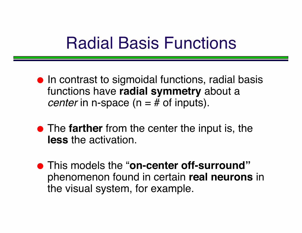
In contrast to sigmoidal functions, radial basisfunctions have radial symmetry about acenter in n-space (n = # of inputs).

The farther from the center the input is, theless the activation.

This models the “on-center off-surround”phenomenon found in certain real neurons inthe visual system, for example.

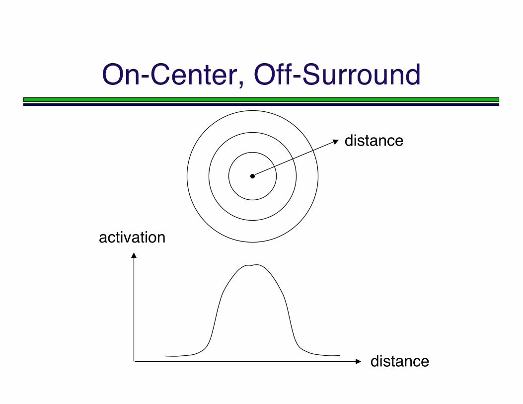
On-Center, Off-Surround

activation

distance

distance

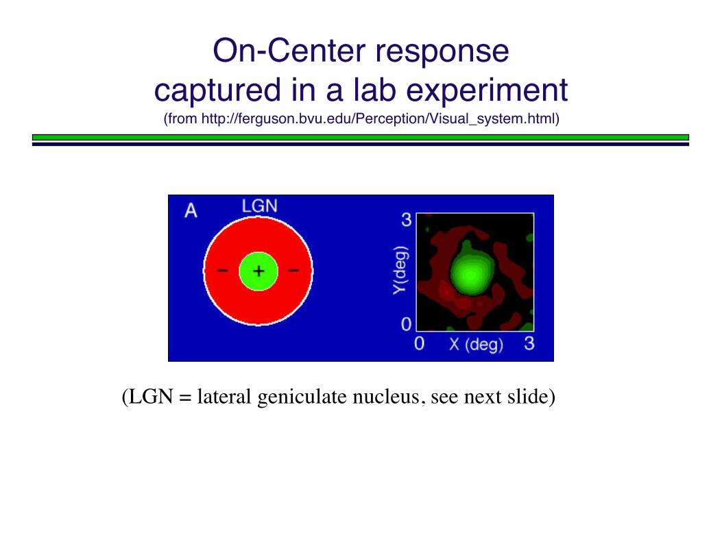
On-Center responsecaptured in a lab experiment

(from http://ferguson.bvu.edu/Perception/Visual_system.html)

(LGN = lateral geniculate nucleus, see next slide)

LGN description,from http://www.science.gmu.edu/~nbanerje/csi801/report_html.htm

LGN is a folded sheet of neurons (1.5 million cells), aboutthe size of a credit card but about three times as thick, foundon each side of the brain.

The ganglion cells of the LGN transform the signals into atemporal series of discrete electrical impulses called actionpotentials or spikes.

The ganglion cell responses are measured by recording thetemporal pattern of action potentials caused by lightstimulation.

(continued)

LGN description,from http://www.science.gmu.edu/~nbanerje/csi801/report_html.htm

The receptive fields of the LGN neurons are circularly symmetric andhave the same center-surround organization.

The algebraic sum of the center and surround mechanisms has a vagueresemblance to a sombrero with a tall peak, so this model of the receptivefield is sometimes called "Mexican-hat model."

When the spatial profiles of center and surround mechanisms can bedescribed by Gaussian functions the model is referred to as the"difference-of-Gaussians" model.

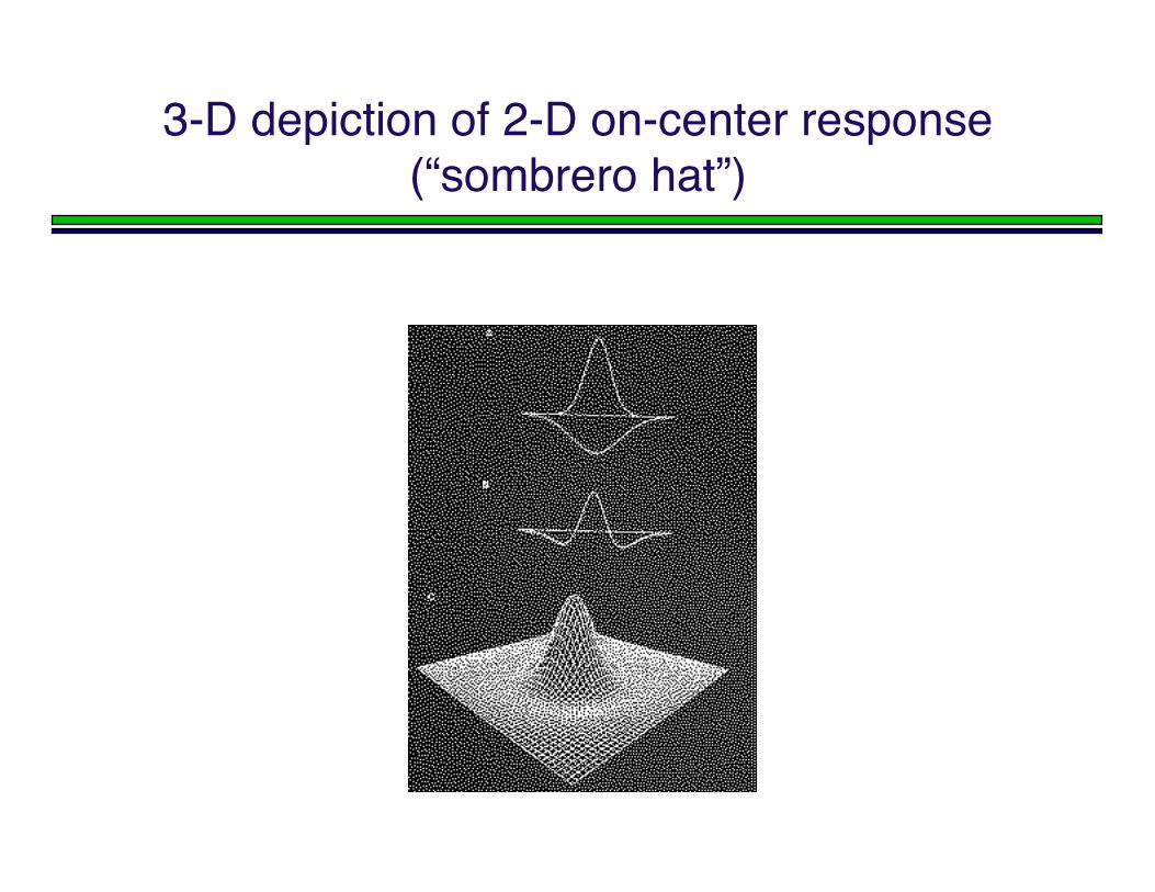
3-D depiction of 2-D on-center response(“sombrero hat”)

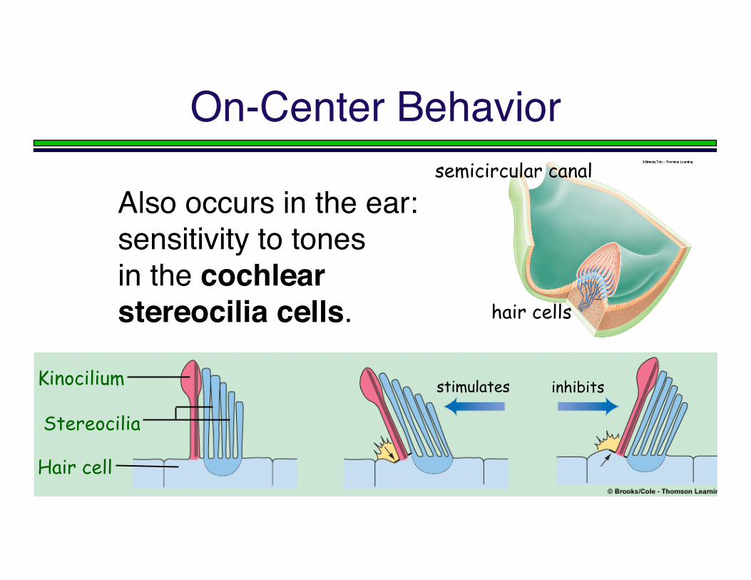
On-Center Behavior

Also occurs in the ear:sensitivity to tonesin the cochlearstereocilia cells.

Kinocilium

Stereocilia

Hair cell

stimulates inhibits

semicircular canal

hair cells

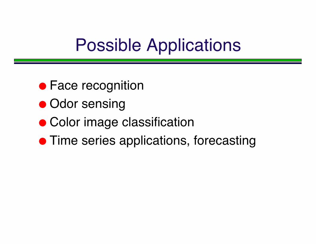
Possible Applications

Face recognition Odor sensing Color image classification Time series applications, forecasting

Modeling

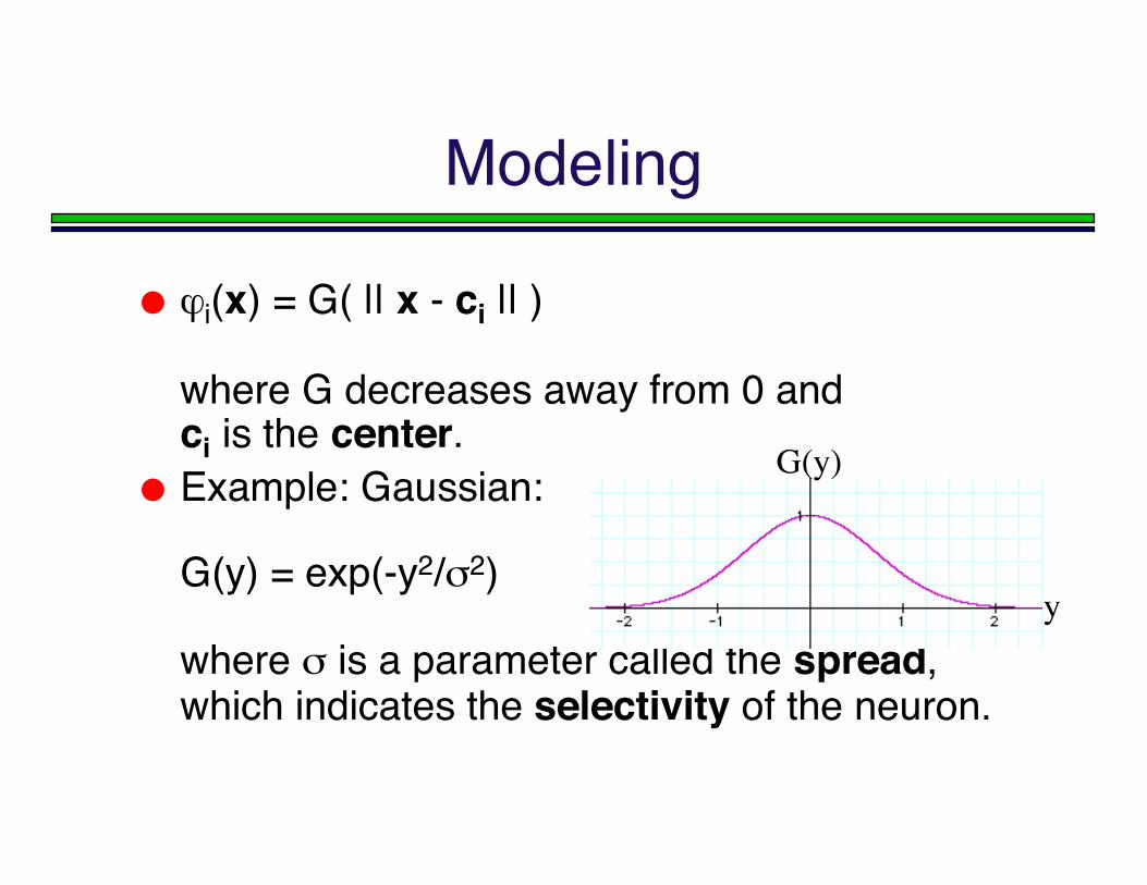
ϕi(x) = G( || x - ci || )

where G decreases away from 0 andci is the center.

Example: Gaussian:

G(y) = exp(-y2/σ2)

where σ is a parameter called the spread,which indicates the selectivity of the neuron.

y

G(y)

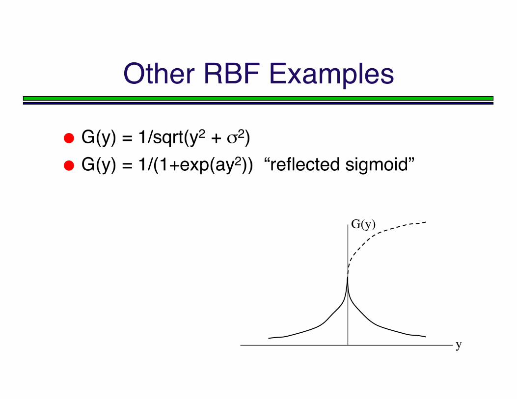
Other RBF Examples

G(y) = 1/sqrt(y2 + σ2) G(y) = 1/(1+exp(ay2)) “reflected sigmoid”

y

G(y)

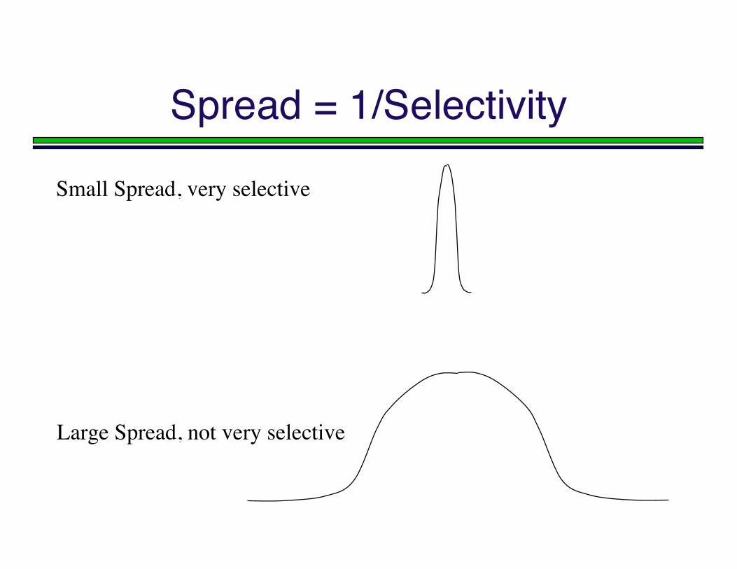
Spread = 1/Selectivity

Small Spread, very selective

Large Spread, not very selective

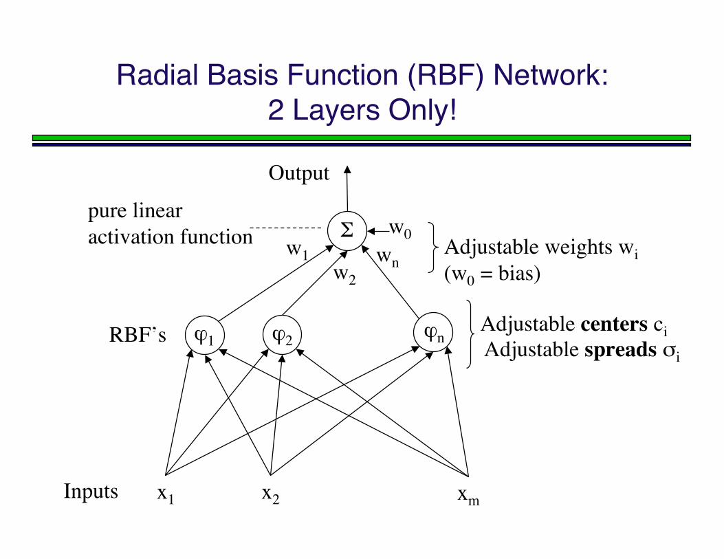
Radial Basis Function (RBF) Network:2 Layers Only!

ϕ1 ϕ2 ϕn

Σ

x1 x2 xm

w1w2

wn

Inputs

Output

Adjustable weights wi (w0 = bias)

pure linearactivation function

RBF’s Adjustable centers ci

Adjustable spreads σi

w0

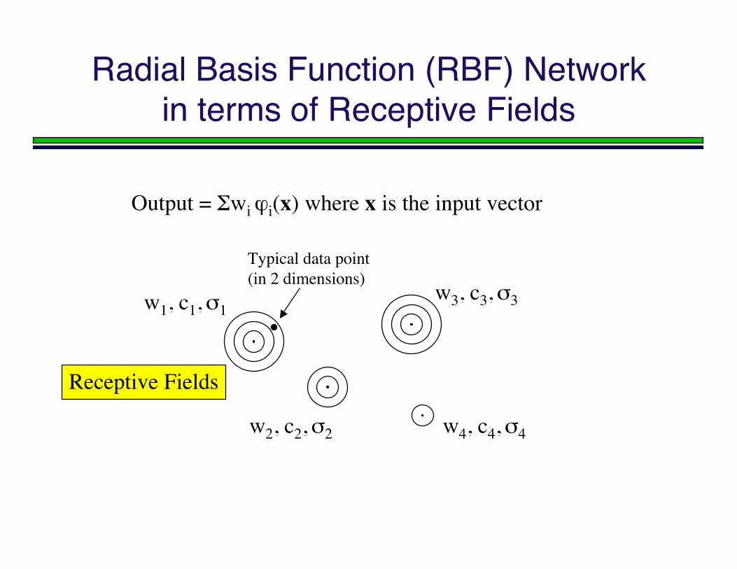
Radial Basis Function (RBF) Networkin terms of Receptive Fields

Output = Σwi ϕi(x) where x is the input vector

w1, c1, σ1

w2, c2, σ2

w3, c3, σ3

w4, c4, σ4

Typical data point (in 2 dimensions)

Receptive Fields

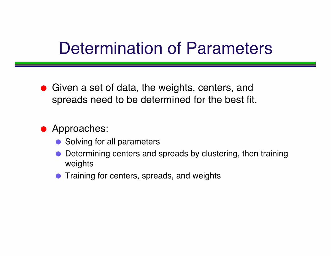
Determination of Parameters

Given a set of data, the weights, centers, andspreads need to be determined for the best fit.

Approaches: Solving for all parameters Determining centers and spreads by clustering, then training

weights Training for centers, spreads, and weights

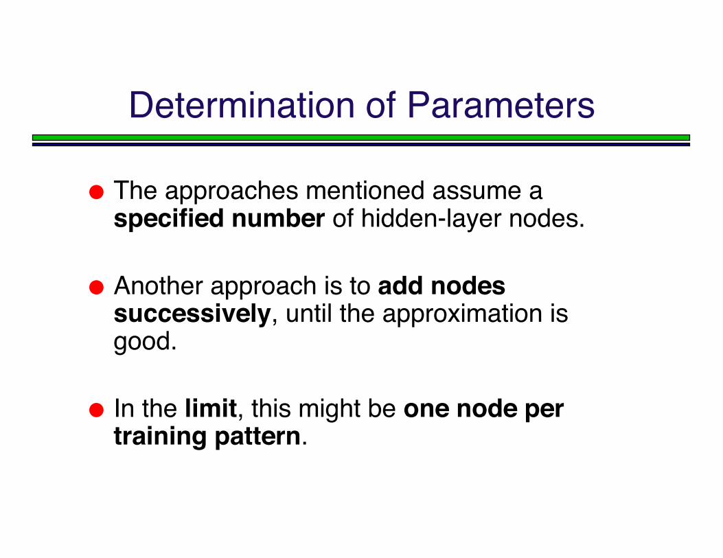
Determination of Parameters

The approaches mentioned assume aspecified number of hidden-layer nodes.

Another approach is to add nodessuccessively, until the approximation isgood.

In the limit, this might be one node pertraining pattern.

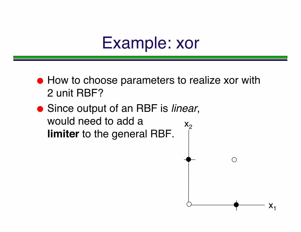
Example: xor

How to choose parameters to realize xor with2 unit RBF?

Since output of an RBF is linear,would need to add alimiter to the general RBF.

x1

x2

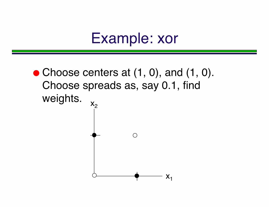
Example: xor

Choose centers at (1, 0), and (1, 0).Choose spreads as, say 0.1, findweights.

x1

x2

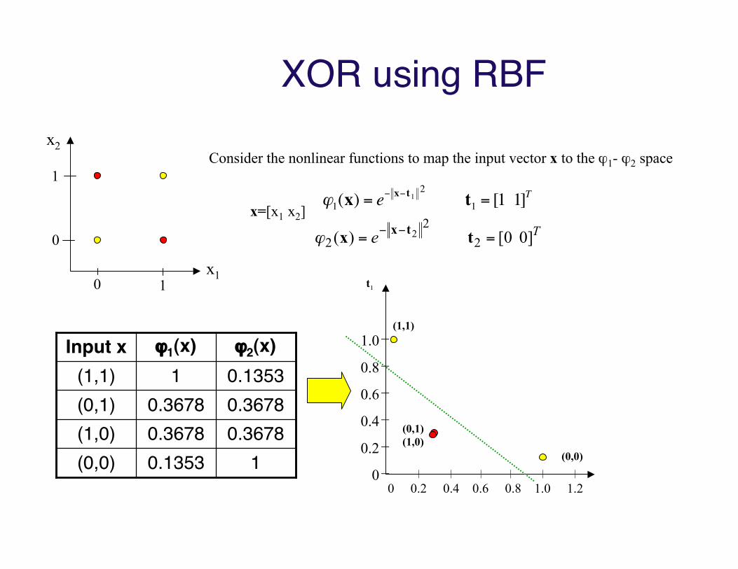
XOR using RBF

0 1

0

1Consider the nonlinear functions to map the input vector x to the ϕ1- ϕ2 space

!

"1(x) = e# x#t12 t1 = [1 1]T

Te ]0 0[ )( 22

22 == !! tx tx"

x1

x2

x=[x1 x2]

10.1353(0,0)0.36780.3678(1,0)0.36780.3678(0,1)0.13531(1,1)ϕ2(x)ϕ1(x)Input x

0 0.2 0.4 0.6 0.8 1.0 1.2 | | | | | |

_

_

_

_

_

_

1.0

0.8

0.6

0.4

0.2

0(0,0)

(1,1)

(0,1)(1,0)

!

t1

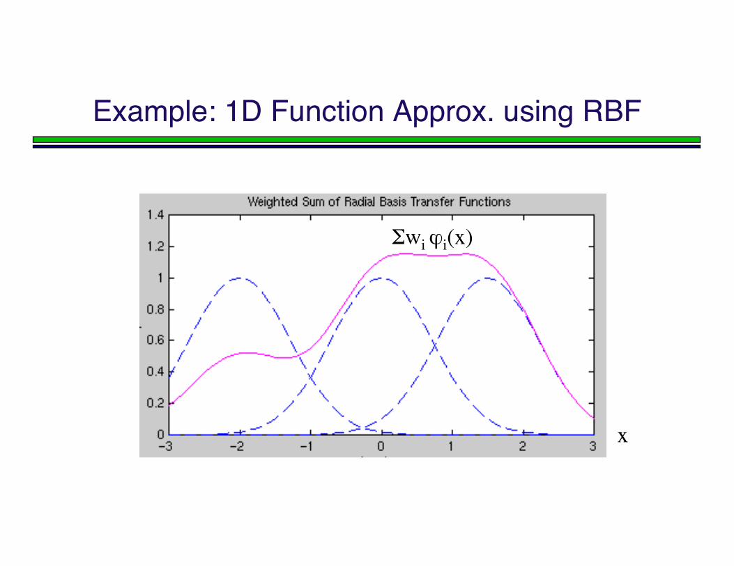
Example: 1D Function Approx. using RBF

Σwi ϕi(x)

x

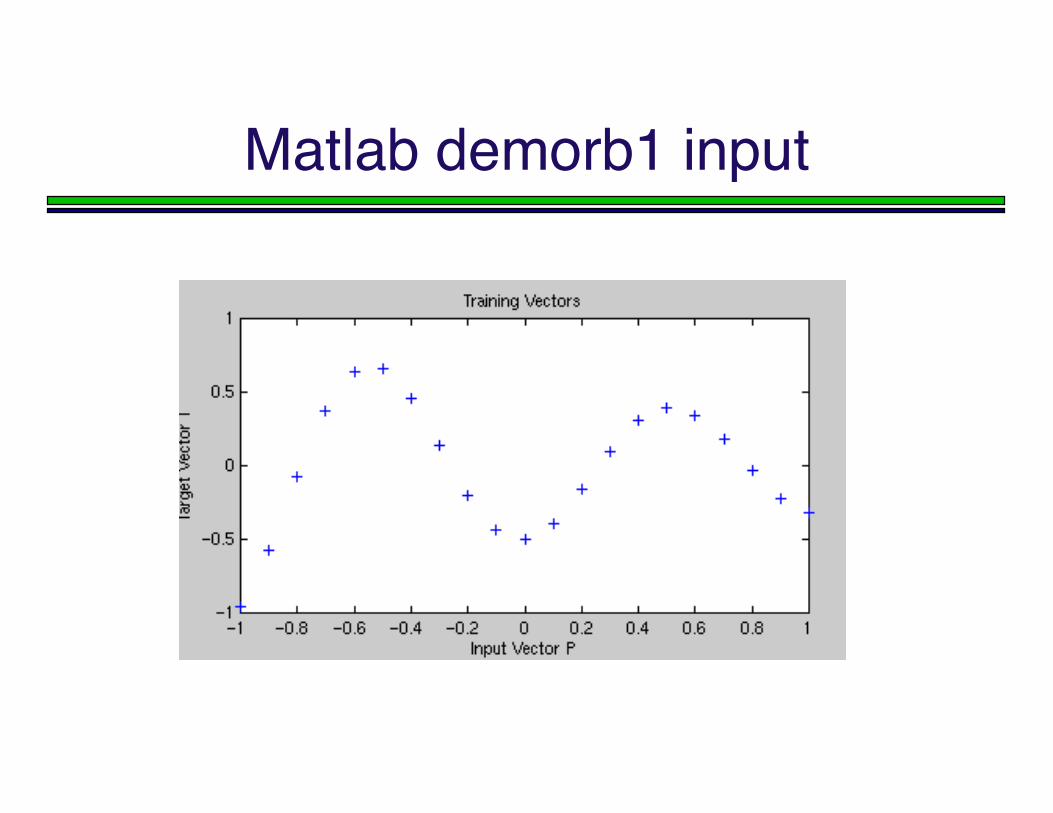
Matlab demorb1 input

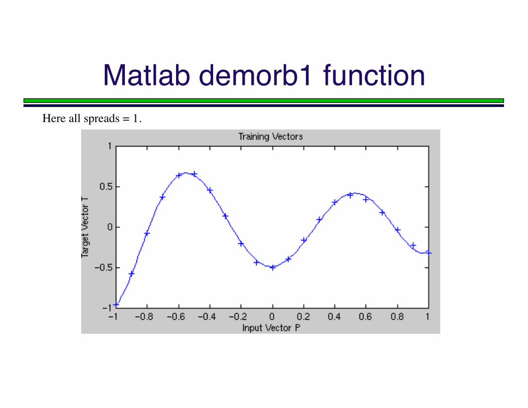
Matlab demorb1 functionHere all spreads = 1.

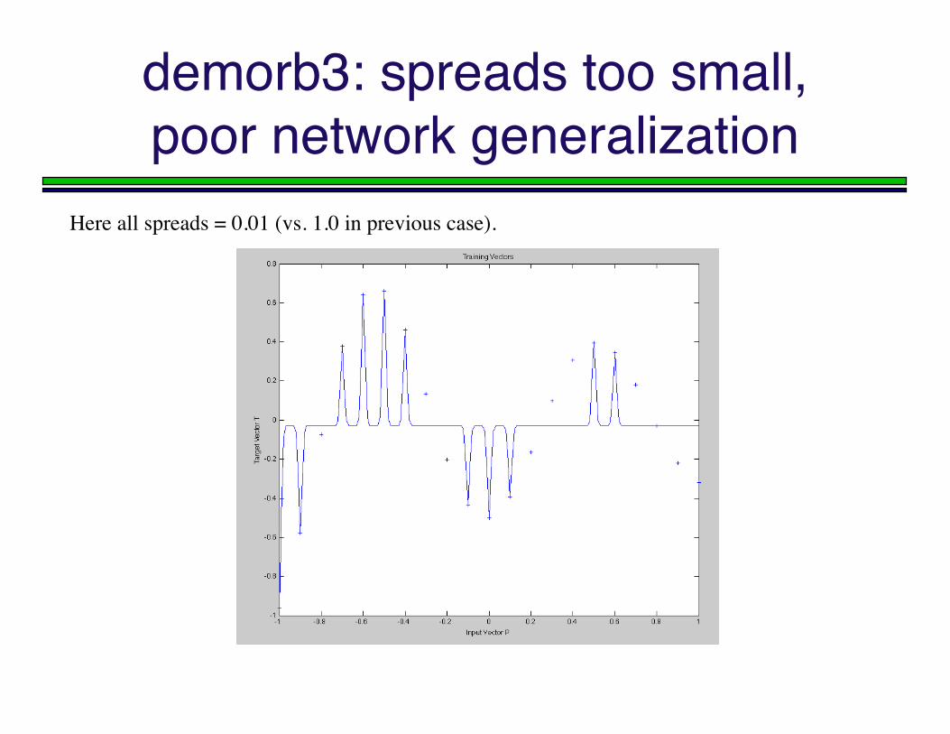
demorb3: spreads too small,poor network generalization

Here all spreads = 0.01 (vs. 1.0 in previous case).

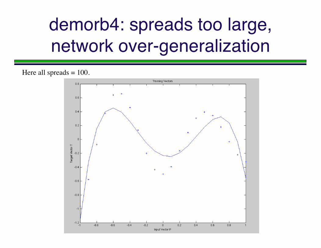
demorb4: spreads too large,network over-generalization

Here all spreads = 100.

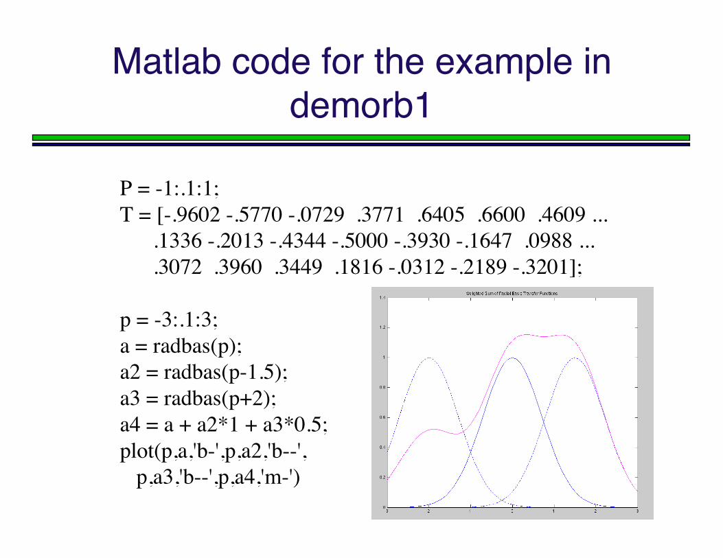
Matlab code for the example indemorb1

P = -1:.1:1;T = [-.9602 -.5770 -.0729 .3771 .6405 .6600 .4609 ... .1336 -.2013 -.4344 -.5000 -.3930 -.1647 .0988 ... .3072 .3960 .3449 .1816 -.0312 -.2189 -.3201];

p = -3:.1:3;a = radbas(p);a2 = radbas(p-1.5);a3 = radbas(p+2);a4 = a + a2*1 + a3*0.5;plot(p,a,'b-',p,a2,'b--', p,a3,'b--',p,a4,'m-')

Bias-Variance Dilemma

“Bias-variance dilemma” applies to thechoice of spreads.

ref. Neural and Adaptive Systems, Jose C.Principe, Neil R. Euliano, Curt Lefebvre

RBF Properties

RBF networks tend to have goodinterpolation properties,

but not as good extrapolation properties asMulti-Level Perceptrons (MLPs).

It seems pretty obvious why.

For extrapolation, using a given number ofneurons, an MLP could be a much better fit.

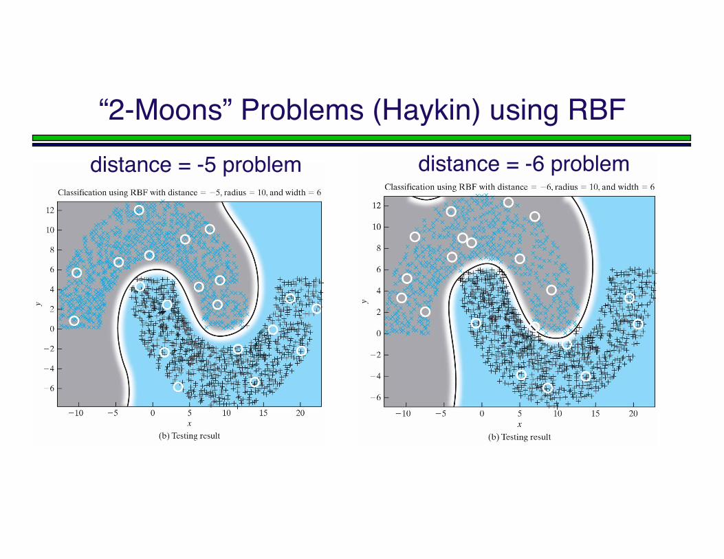
“2-Moons” Problems (Haykin) using RBFdistance = -5 problem distance = -6 problem

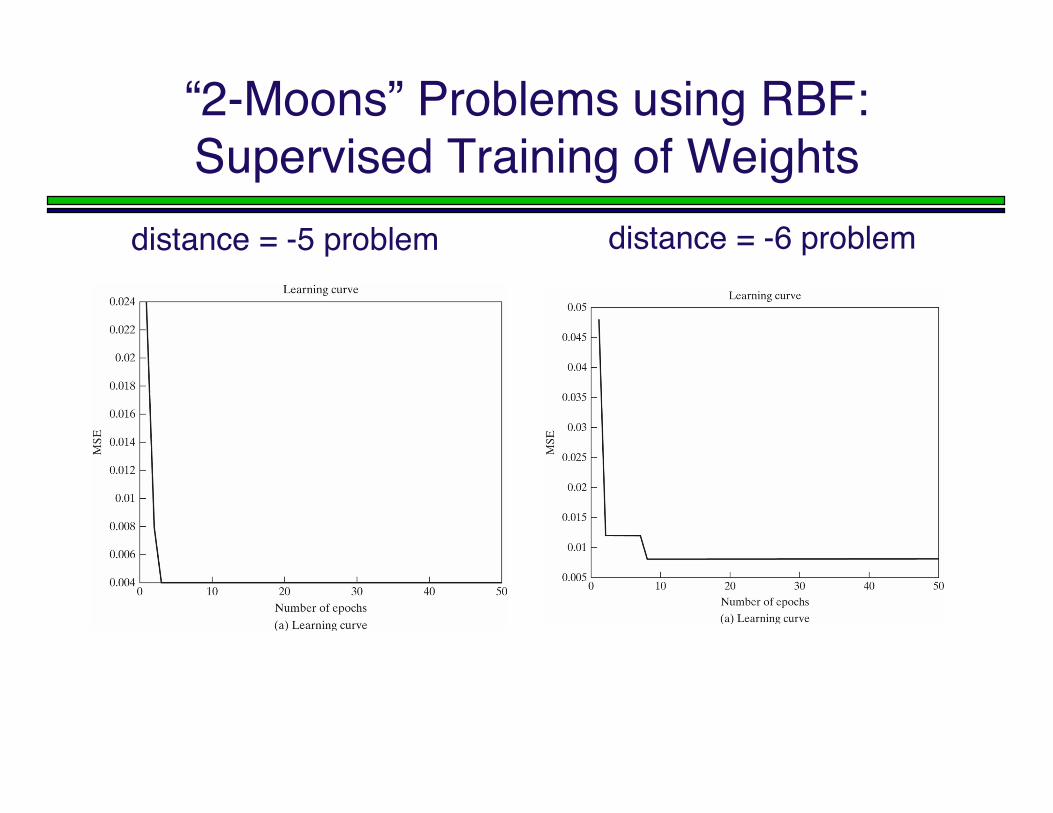
“2-Moons” Problems using RBF:Supervised Training of Weights

distance = -5 problem distance = -6 problem

Training-Performance andUniversality

With proper setup, RBFNs can train in timeorders of magnitude faster thanbackpropagation.

RBFNs enjoy the same universalapproximation properties as MLPs: givensufficient neurons, any reasonable functioncan be approximated (with just 2 layers).

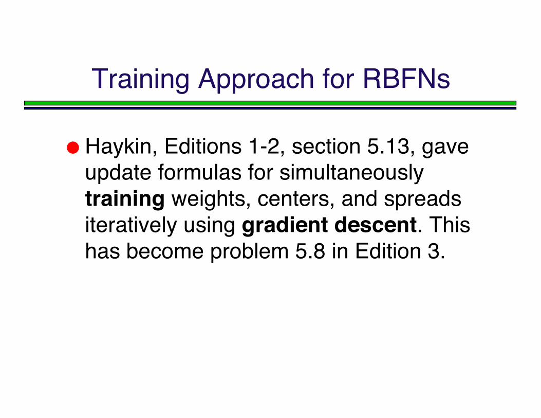
Training Approach for RBFNs

Haykin, Editions 1-2, section 5.13, gaveupdate formulas for simultaneouslytraining weights, centers, and spreadsiteratively using gradient descent. Thishas become problem 5.8 in Edition 3.

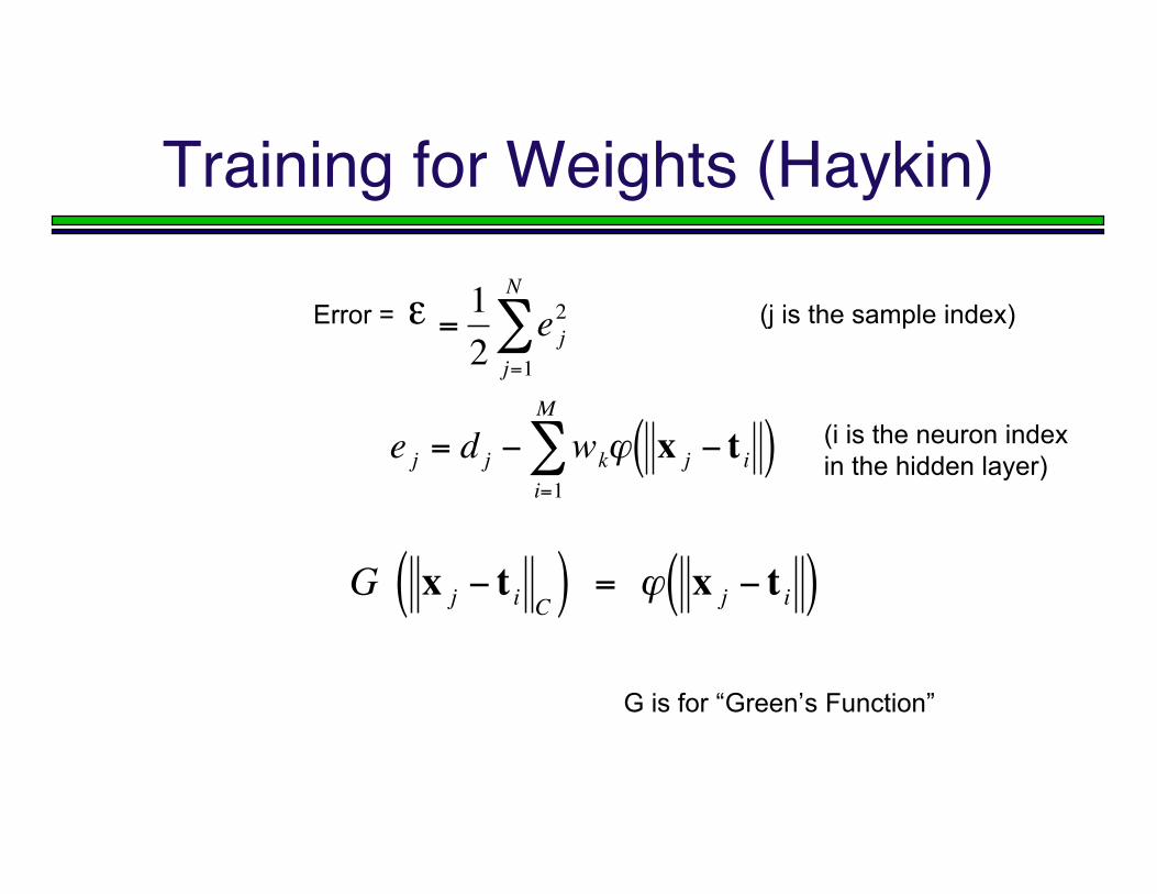
Training for Weights (Haykin)

!

=12

e j2

j=1

N

"

e j = d j # wk$ x j # t i( )i=1

M

"

Error = ε

!

G x j " t i C( ) = # x j " t i( )

(j is the sample index)

(i is the neuron indexin the hidden layer)

G is for “Green’s Function”

(j is the sample index, i is the weight index)

G’ is the derivative of the “Green’s Function”

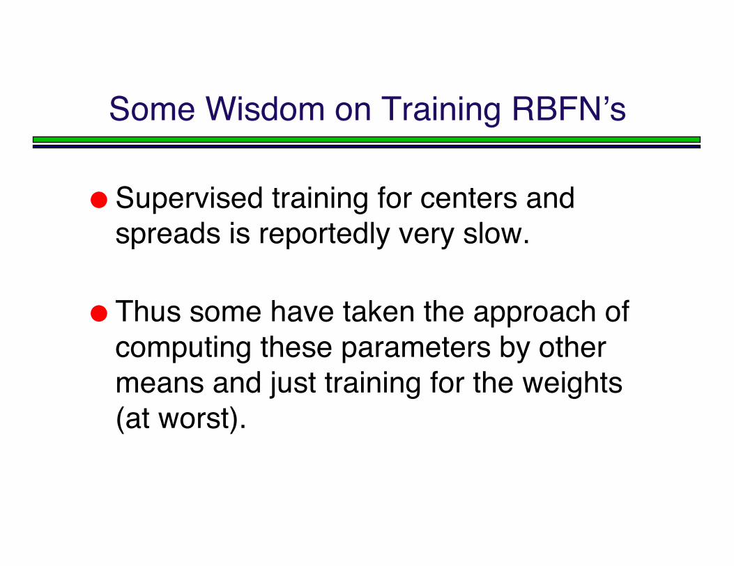
Some Wisdom on Training RBFNʼs

Supervised training for centers andspreads is reportedly very slow.

Thus some have taken the approach ofcomputing these parameters by othermeans and just training for the weights(at worst).

A Solving Approach for RBF

Suppose we are willing to use oneneuron per training sample point.

Choose the N data points themselvesas centers.

Assume the spreads σi are given.

A Solving Approach for RBF

It then only remains to find the weights.

Define ϕji = ϕ(|| xi -xj ||) where ϕ is the radialbasis function, xi, xj are training samples.

The matrix Φ of values ϕji is called theinterpolation matrix.

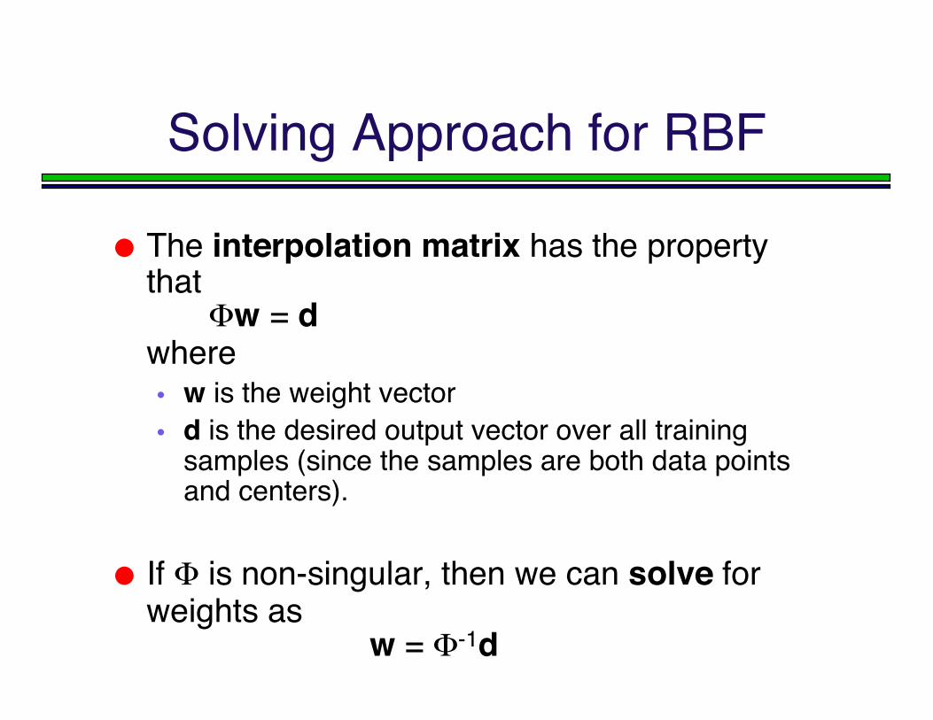
Solving Approach for RBF

The interpolation matrix has the propertythat

Φw = dwhere• w is the weight vector• d is the desired output vector over all training

samples (since the samples are both data pointsand centers).

If Φ is non-singular, then we can solve forweights as

w = Φ-1d

Solving Approach for RBFNs

Micchelliʼs Theorem says that if the points xiare distinct, then the Φ matrix will be non-singular (it is square, by construction).

Ref: Mhaskar and Micchelli, Approximation bysuperposition of sigmoidal and radial basisfunctions, Advances in Applied Mathematics,13, 350-373, 1992.

Non-Square Case

Having one RBF per training point maybe too costly.

It may also cause over-fitting.

Training in the Presence of Noise

Noise in the training set can be good; itcan make the resulting network, whichhas learned to “average” noise in, morerobust.

However, with too many neurons, anetwork can over-train to “learn thenoise”.

Regularization by Weight Decay

Can use the Weight Decay method to prune anRBF: At each update, a small amount is deducted from each

weight.

Weights that are constantly being updated will end up with anon-0 value, while others will go to 0 and can be eliminated.

The resulting network is less trained to the noise.

Weight Decay is a form of “regularization”

Selecting Centers by Clustering

One center per training sample may be over-kill.

There are ways to select centers asrepresentatives among clusters, given afixed number of representatives.

We will give and example, and discuss thesefurther under “unsupervised learning” andcompetitive methods.

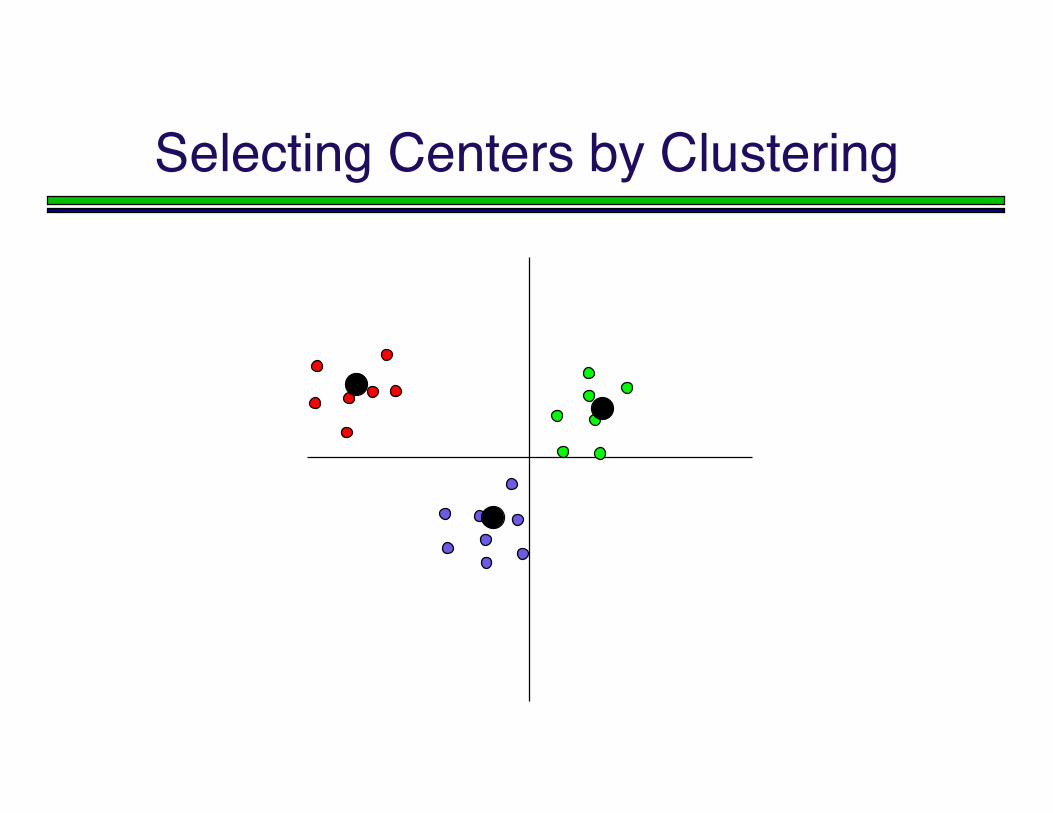
Selecting Centers by Clustering

This determines which points belong to which clusters, as wellas the centers of those clusters.

The desired number k of clusters is specified.

Initialize k centers, e.g. by choosing them to be k distinct datapoints.

Repeat For each data point, determine which center is closest. This

determines each pointʼs cluster for the current iteration. Compute the centroid (mean) of the points in each cluster. Make

this the centers for the next iteration.until centers donʼt differ appreciably from their previous value.

“k-means clustering”(MacQueen 1967)

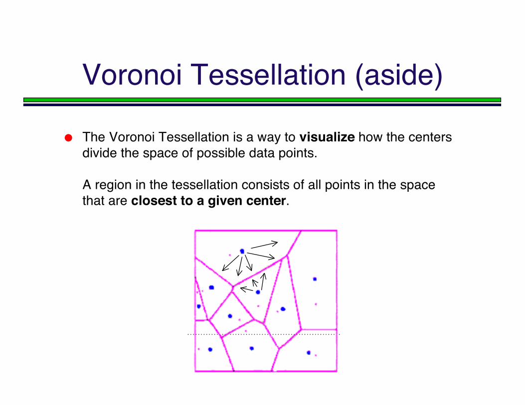
Voronoi Tessellation (aside)

The Voronoi Tessellation is a way to visualize how the centersdivide the space of possible data points.

A region in the tessellation consists of all points in the spacethat are closest to a given center.

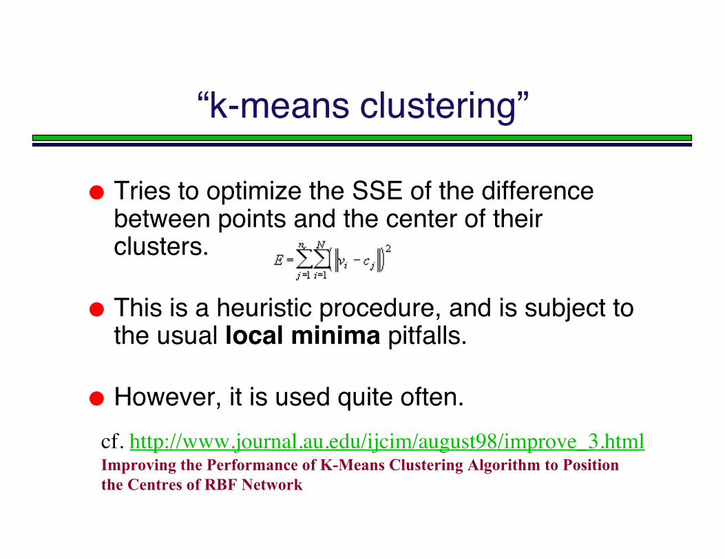
“k-means clustering”

Tries to optimize the SSE of the differencebetween points and the center of theirclusters.

This is a heuristic procedure, and is subject tothe usual local minima pitfalls.

However, it is used quite often.cf. http://www.journal.au.edu/ijcim/august98/improve_3.htmlImproving the Performance of K-Means Clustering Algorithm to Position the Centres of RBF Network

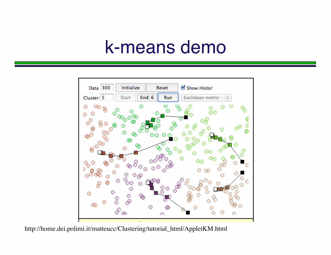
k-means demo

http://home.dei.polimi.it/matteucc/Clustering/tutorial_html/AppletKM.html

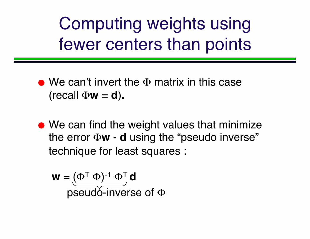
Computing weights usingfewer centers than points

We canʼt invert the Φ matrix in this case(recall Φw = d).

We can find the weight values that minimizethe error Φw - d using the “pseudo inverse”technique for least squares :

w = (ΦT Φ)-1 ΦT d pseudo-inverse of Φ

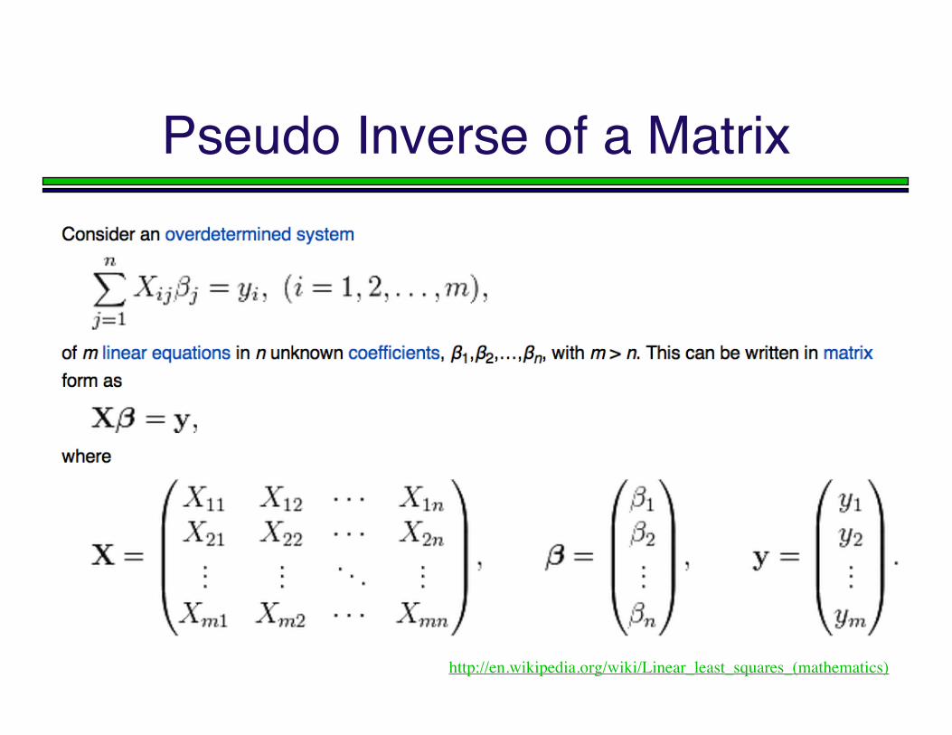
Pseudo Inverse of a Matrix

http://en.wikipedia.org/wiki/Linear_least_squares_(mathematics)

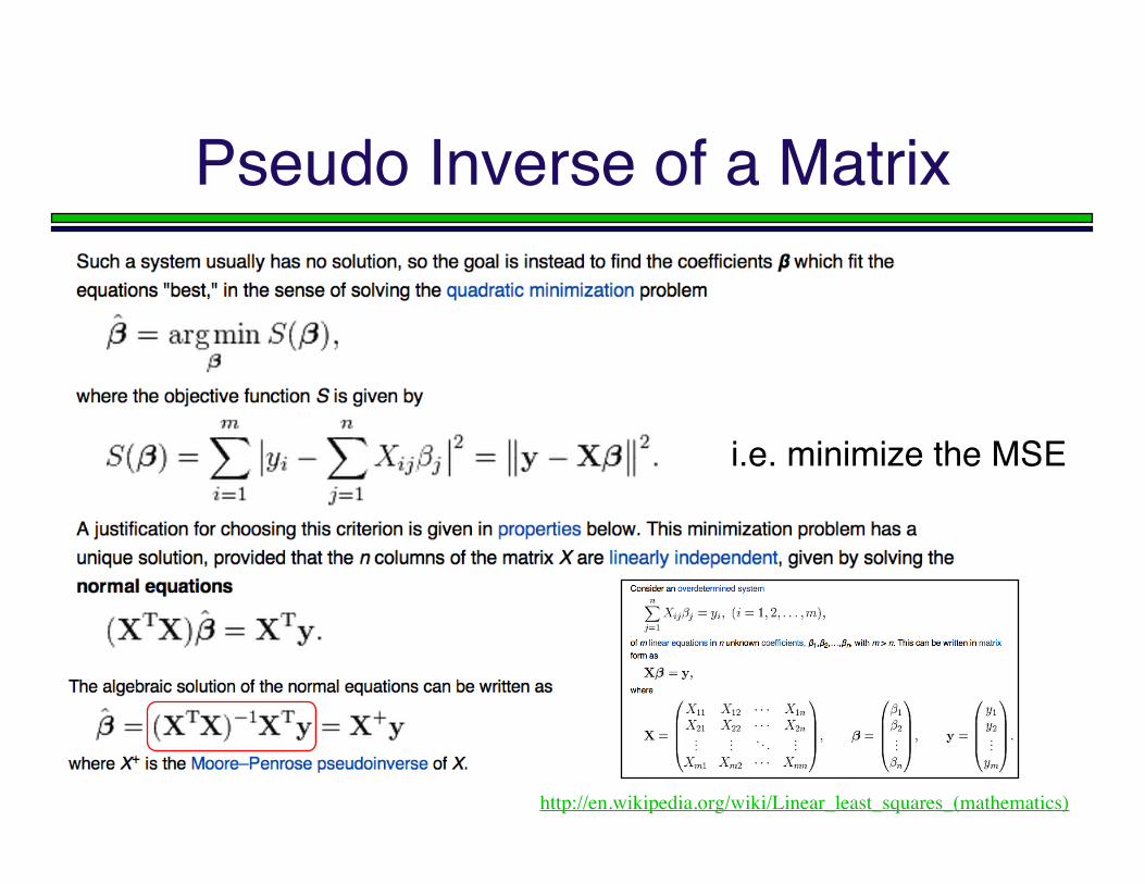
Pseudo Inverse of a Matrix

http://en.wikipedia.org/wiki/Linear_least_squares_(mathematics)

i.e. minimize the MSE

Setting spreads

Once centers are known, spreads canbe set, e.g. by selecting the averagedistance between center and the cclosest points in the cluster (e.g. c = 5).

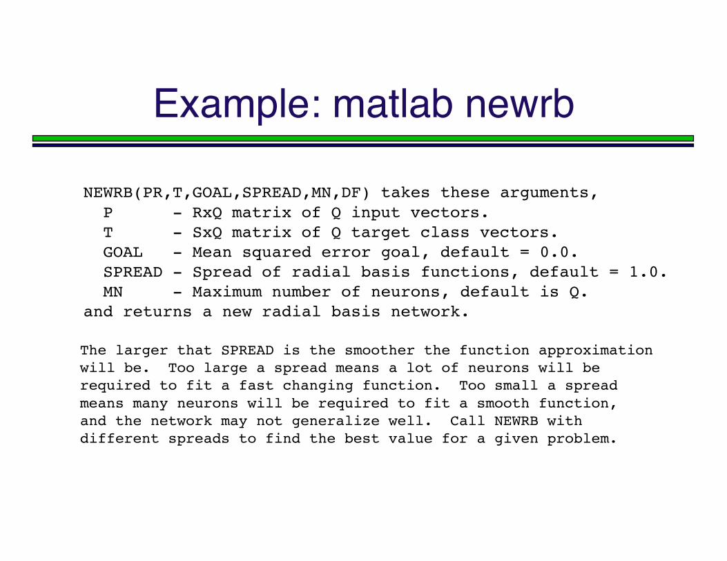
Example: matlab newrb

NEWRB(PR,T,GOAL,SPREAD,MN,DF) takes these arguments, P - RxQ matrix of Q input vectors. T - SxQ matrix of Q target class vectors. GOAL - Mean squared error goal, default = 0.0. SPREAD - Spread of radial basis functions, default = 1.0. MN - Maximum number of neurons, default is Q. and returns a new radial basis network.

The larger that SPREAD is the smoother the function approximation will be. Too large a spread means a lot of neurons will be required to fit a fast changing function. Too small a spread means many neurons will be required to fit a smooth function, and the network may not generalize well. Call NEWRB with different spreads to find the best value for a given problem.

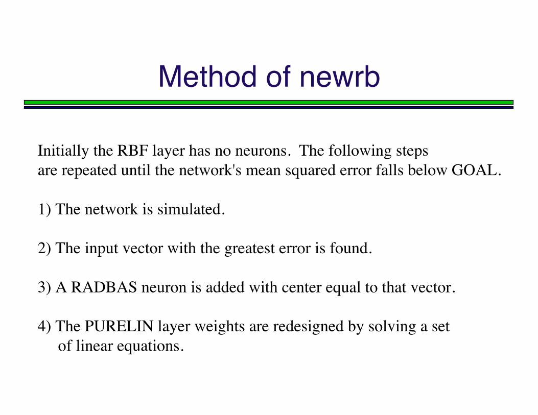
Method of newrb

Initially the RBF layer has no neurons. The following stepsare repeated until the network's mean squared error falls below GOAL.

1) The network is simulated.

2) The input vector with the greatest error is found.

3) A RADBAS neuron is added with center equal to that vector.

4) The PURELIN layer weights are redesigned by solving a set of linear equations.

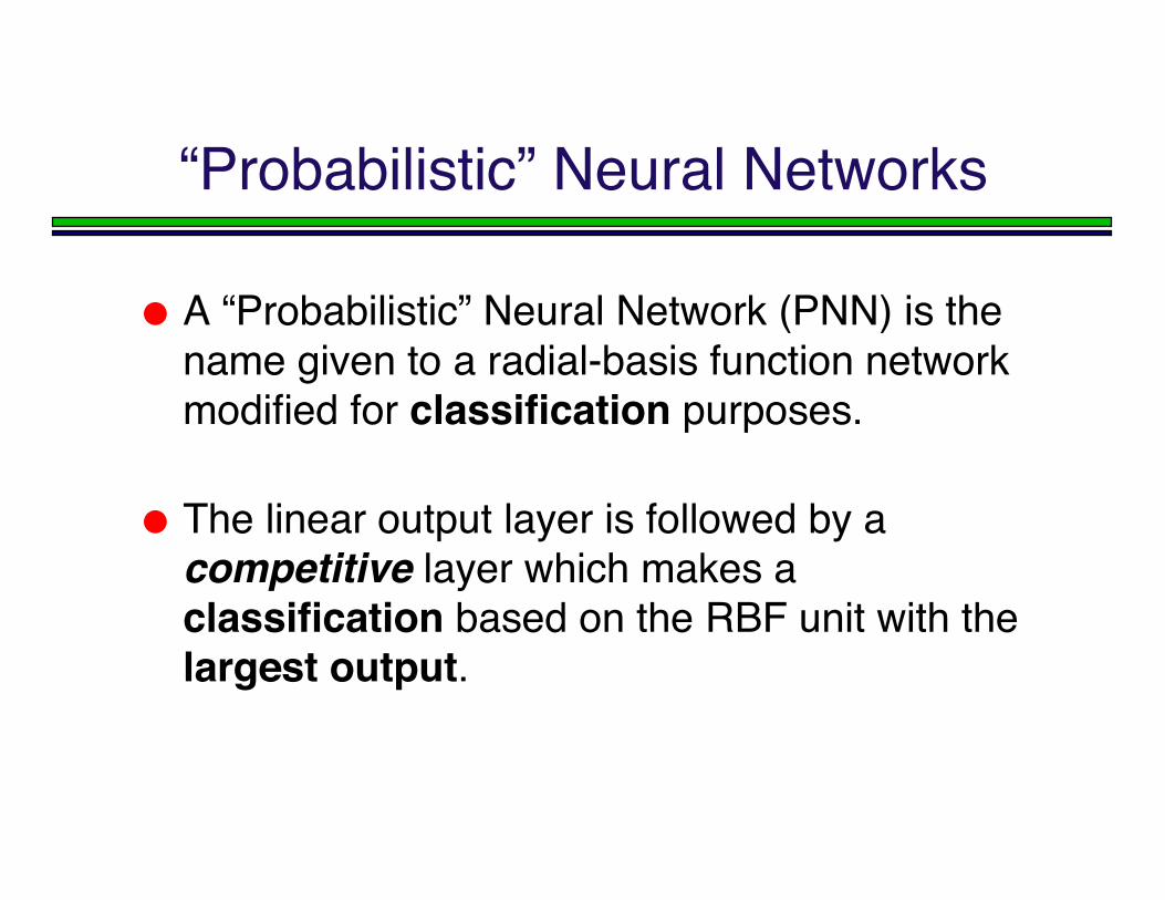
“Probabilistic” Neural Networks

A “Probabilistic” Neural Network (PNN) is thename given to a radial-basis function networkmodified for classification purposes.

The linear output layer is followed by acompetitive layer which makes aclassification based on the RBF unit with thelargest output.

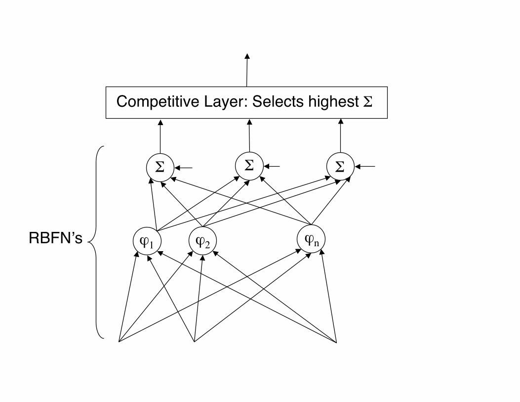
ϕ1 ϕ2 ϕn

ΣΣ Σ

Competitive Layer: Selects highest Σ

RBFNʼs

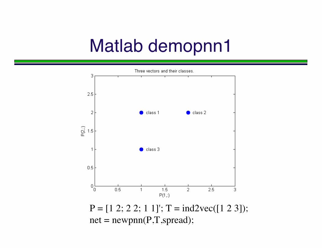
Matlab demopnn1

P = [1 2; 2 2; 1 1]'; T = ind2vec([1 2 3]);net = newpnn(P,T,spread);

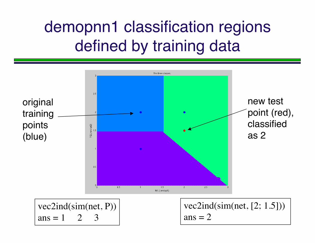
demopnn1 classification regionsdefined by training data

vec2ind(sim(net, P))ans = 1 2 3

vec2ind(sim(net, [2; 1.5])) ans = 2

new testpoint (red),classifiedas 2

originaltrainingpoints(blue)

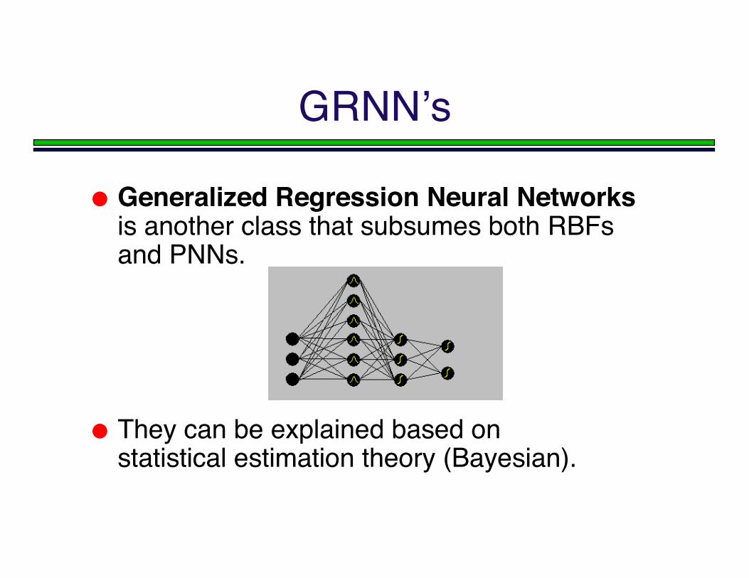
GRNNʼs

Generalized Regression Neural Networksis another class that subsumes both RBFsand PNNs.

They can be explained based onstatistical estimation theory (Bayesian).

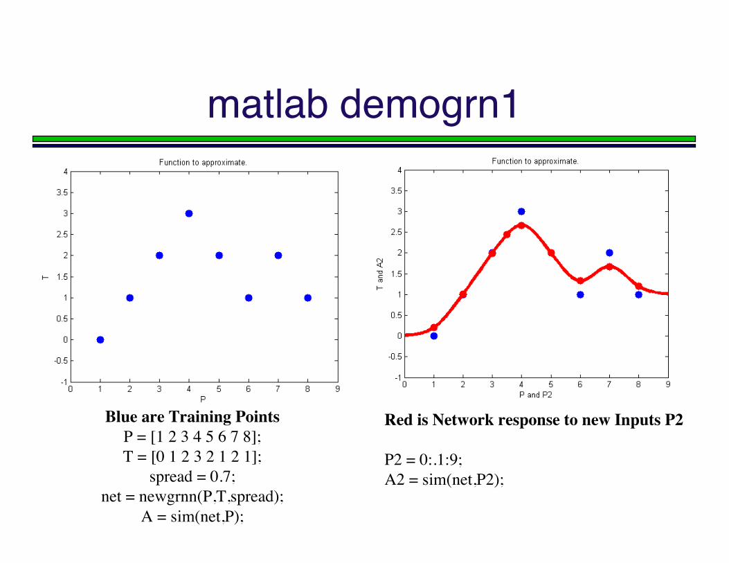
matlab demogrn1

Blue are Training PointsP = [1 2 3 4 5 6 7 8];T = [0 1 2 3 2 1 2 1];

spread = 0.7;net = newgrnn(P,T,spread);

A = sim(net,P);

Red is Network response to new Inputs P2

P2 = 0:.1:9;A2 = sim(net,P2);

Related Topic to GRNN

Support Vector Machines (SVMs)to be discussed

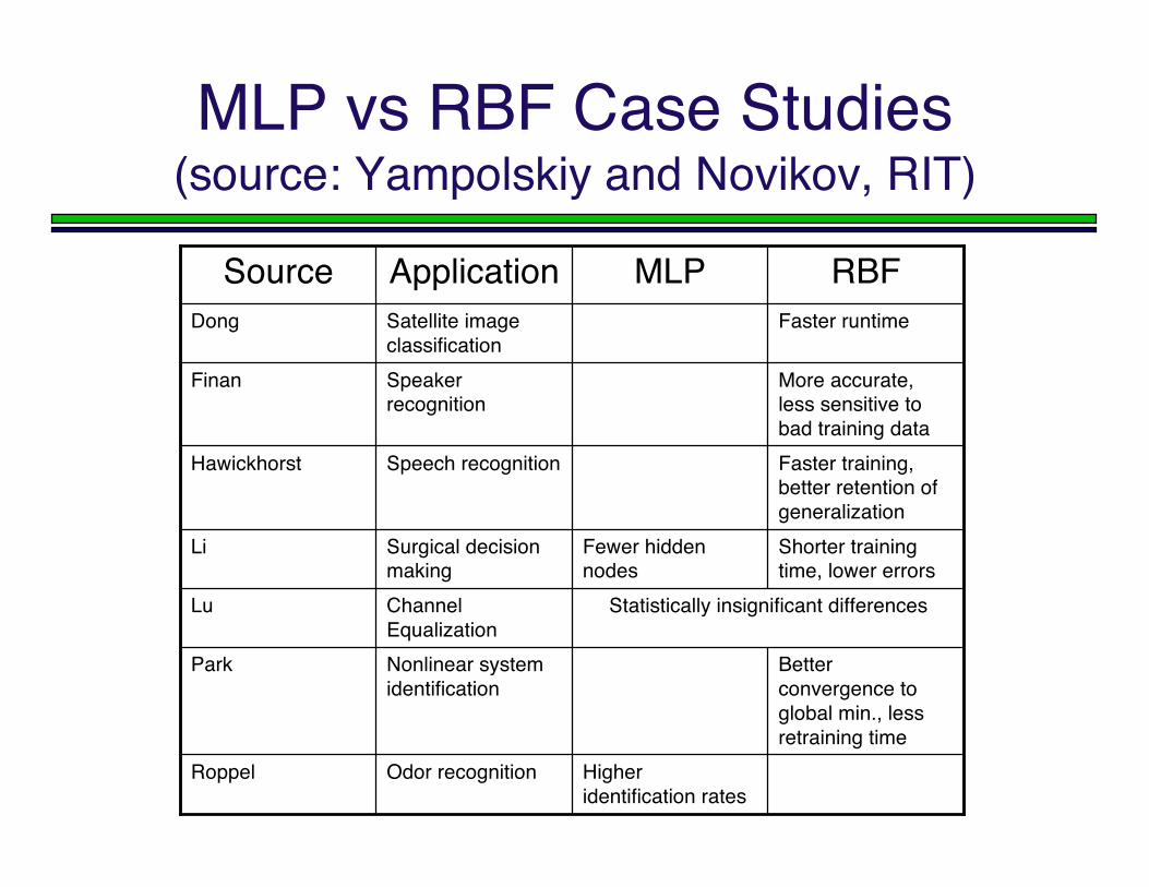
MLP vs RBF Case Studies(source: Yampolskiy and Novikov, RIT)

Higheridentification rates

Odor recognitionRoppel

Betterconvergence toglobal min., lessretraining time

Nonlinear systemidentification

Park

Statistically insignificant differencesChannelEqualization

Lu

Shorter trainingtime, lower errors

Fewer hiddennodes

Surgical decisionmaking

Li

Faster training,better retention ofgeneralization

Speech recognitionHawickhorst

More accurate,less sensitive tobad training data

Speakerrecognition

Finan

Faster runtimeSatellite imageclassification

Dong

RBFMLPApplicationSource

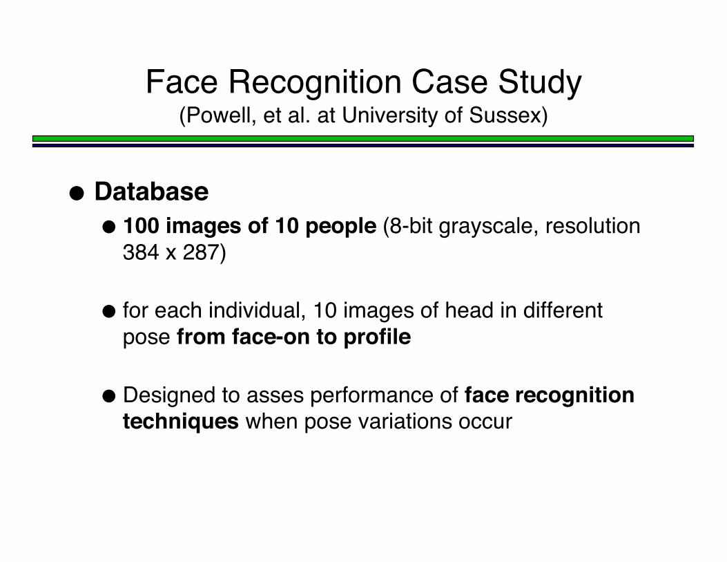
Database 100 images of 10 people (8-bit grayscale, resolution

384 x 287)

for each individual, 10 images of head in differentpose from face-on to profile

Designed to asses performance of face recognitiontechniques when pose variations occur

Face Recognition Case Study(Powell, et al. at University of Sussex)

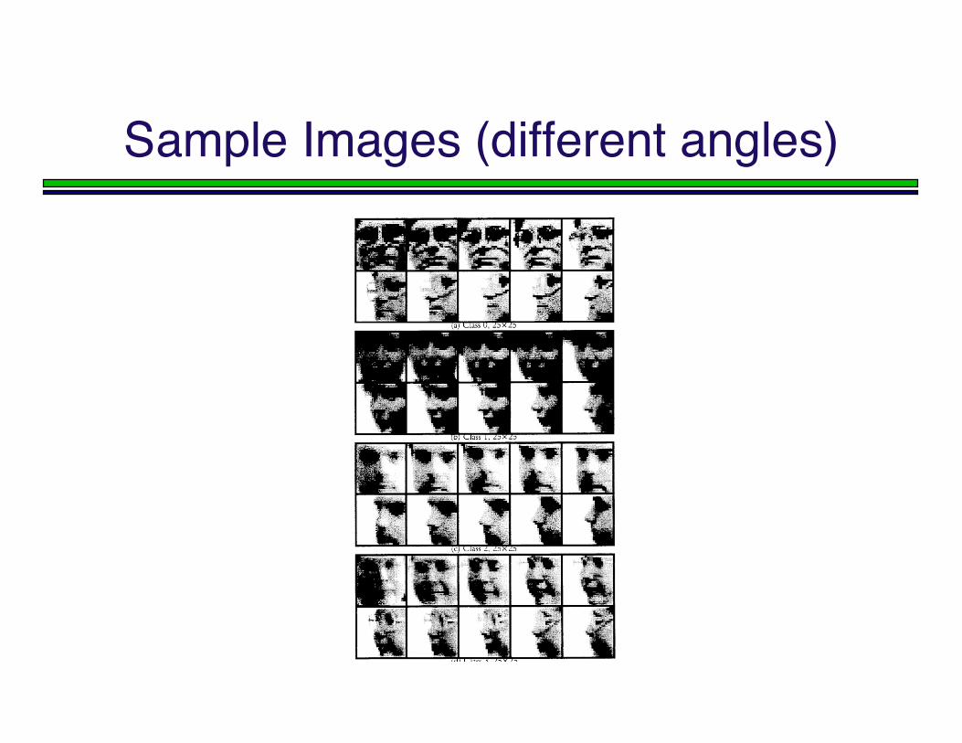
Sample Images (different angles)

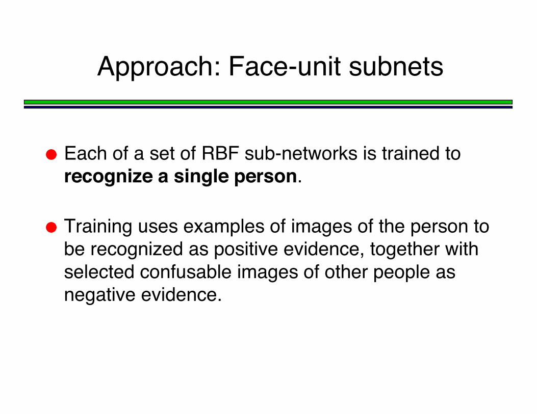
Approach: Face-unit subnets

Each of a set of RBF sub-networks is trained torecognize a single person.

Training uses examples of images of the person tobe recognized as positive evidence, together withselected confusable images of other people asnegative evidence.

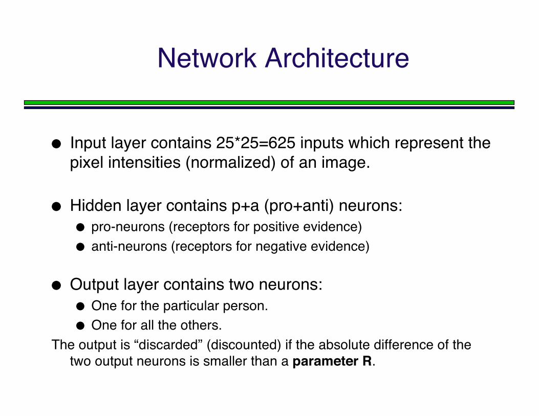
Network Architecture

Input layer contains 25*25=625 inputs which represent thepixel intensities (normalized) of an image.

Hidden layer contains p+a (pro+anti) neurons: pro-neurons (receptors for positive evidence) anti-neurons (receptors for negative evidence)

Output layer contains two neurons: One for the particular person. One for all the others.

The output is “discarded” (discounted) if the absolute difference of thetwo output neurons is smaller than a parameter R.

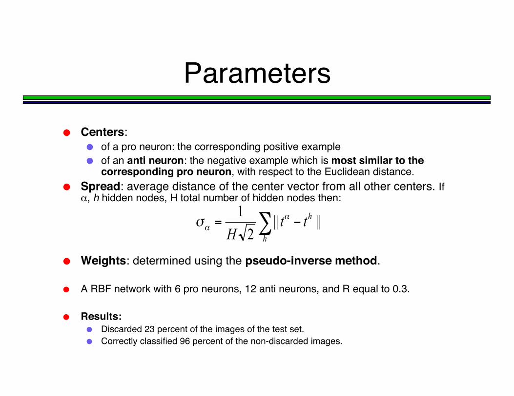
Parameters

Centers: of a pro neuron: the corresponding positive example of an anti neuron: the negative example which is most similar to the

corresponding pro neuron, with respect to the Euclidean distance. Spread: average distance of the center vector from all other centers. If

α, h hidden nodes, H total number of hidden nodes then:

Weights: determined using the pseudo-inverse method.

A RBF network with 6 pro neurons, 12 anti neurons, and R equal to 0.3.

Results: Discarded 23 percent of the images of the test set. Correctly classified 96 percent of the non-discarded images.

! "=h

httH

||||21 #

#$