Radial Basis Function Artificial Neural Networks · Radial Basis Function Artificial Neural...

Radial Basis Funct ion Art ificia l Neural Netw orks

An artificial neural network (ANN) is an information-processing paradigm that is designed to emulate some of the observed properties of the mammalian brain. First proposed in the early 1950's it was not until the technology revolution of the 1980's that a multitude of alternative ANN methods were spawned to solve a wide variety of complex real-world problems. Today, the contemporary literature on ANNs is replete with successful reports of applications to problems that are too complex for conventional algorithmic methods or for which an algorithmic specification is too complex for practical implementation. The robustness of the ANN method under difficult modeling conditions is also well documented. For example, ANNs have proven extremely resilient against distortions introduced by noisy data. In short, the ANN paradigm has a developed a track-record as a good pattern recognition engine, a robust classifier, and an expert functional agent in prediction and system modeling where the physical processes are not easily understood or are highly complex.

At the heart of these impressive results is the learning process. The algorithmic learning process is achieved during an iterative training phase where adjustments are made to the synaptic connection weights that exist between the neurons. These connection weights represent the imputed knowledge that is required to solve specific problems.

WinORS supports two basic neural network algorithms. First, there is a basic implementation of the venerable Backpropagation method. The featured neural network in WinORS is from the radial basis function family. Specifically, WinORS supports four versions of the Kajiji-4 radial basis function (RBF) algorithm (see, Kajiji 2000). The user manual for applying the Kajiji-4 method is discussed below.

Open the Sample File

You may open the data file for the example presented here by using the WinORS web folder (File/Open/Web Data-icon on the outlook bar). The data in this file was imported from WinORS supported sites (see the FX and Economics data sub-menu off of the main Data menu). Column B presents the JPY/USD exchange rate where the log rate of return for this same series is presented in column C. Missing values in the yen-dollar exchange rate were estimated by using the menu tree /ACE. Similarly, following a similar menu tree created the ln rate of return data in column C: /ACR. Columns D and E are obtained from the menu tree: /DE. As with the FX data, the log (ln) rate of returns were created by the menu tree /ACR.

Radial Basis Function Artificial Neural Networks Page: 2

Class Notes 01-JUN-06 Copyright: Gordon H. Dash, Jr and Nina Kajiji, all rights reserved. www.ghdash.net

WinORS Variable Types

Row 2 of the WinORS spreadsheet if often refereed to as the 'variable type' row. This row requires a single character identifier that defines the variable (column) to the chosen application. In the case of the radial basis function ANN, WinORS requires two variable types to be set. The dependent variable (sometimes referred to as a target variable in neural network studies) is identified by a variable type of 'D' in row 2. The predictor variables require the variable type of 'I ' along this row. Below, the other required setting to obtain a solution is discussed -- the range of the data. However, we first introduce the dialog box associated with the radial basis function method.

http://www.ghdash.net



RBF Model Execution

To execute the RBF application on the data set given the model specification (the variable types that are set) as specified, follow this menu tree: /ALR




The RBF Dialog Box

The first action to take on the RBF dialog box is to set the data range (*Range) correctly. In the following case, the data range is incorrect for the problem developed as part of this example. Use the backward facing red arrow to roll-up the screen. When in the rolled-up state, use the mouse (or the keyboard) to highlight all cells that should be considered by the solution method.

Highlighting the Range

Here we see that, at a minimum, columns C through Z are included in the highlighted range. This breadth of range setting includes both the target (dependent) variable in column C, as well as the two independent variables in columns F and G, respectively. NOTE: only variables that are in the range with valid 'variable types' along row two will




be considered in the analysis. Highlight down to the last row desired for inclusion in the analysis.

The RBF Dialog Box - Revisited

Once the highlighting is done and you roll-down the form, the dialog box will show the following results. First, notice that the model will be constructed over the range from cell C6 on tab A to cell Z652, tab A, inclusive.

Expert Mode

In order to set the ranges for the Forecast and Table, the check box for Expert Mode must be in the ‘on’ state (see bottom right corner). Although it was not shown, the form was rolled-up for a second time using the backward facing red arrow associated with the Forecast range. In this example the forecast range was set to start at the next available row (653) and only this row (a one-period ahead forecast). NOTE: the forecast range can be blank. That is, it is acceptable to only model the target data (not model and forecast). Finally, the Table is the range over which to build the output table. While it is possible to direct the output to any specific location, it is strongly suggested to leave this setting at its default value.




Data Set Training and Validation Ranges

Start the neural network analysis by apportioning approximately 1/3 (33%) of the data set to the supervised training phase of the analysis. The remaining 2/3 (67%) of the data is automatically assigned to the validation phase. Use the provided spin control to increase (decrease) the allocation between the training and validation sets. Is the default proportion optimal? Unfortunately, this question is still open to debate. In fact, it is a major research issue in the field of study. The objective is to properly train the neural network. An improper training of the neural network may lead to an over-trained network. An over-trained network models both the true variability as well as the noise (error) in the variability of the data. In the current implementation, WinORS does not




support techniques like cross-validation to automate the process of finding the best demarcation point between the training and validation sets.

Data Scaling by Transformation

Data scaling is another important issue in neural network modeling. Currently, WinORS supports the following data transformation (scaling) methods: Standardized – Method 1; Standardized – Method 2; Normalized – Method 1; Normalized – Method 2; and, Uniform.

It is possible to choose whether to apply the chosen transformation method to the target variable. Use the check-box to indicate Yes/No to this decision. The default is Yes - apply the transformation to the target variable.

Algorithmic Method

Choose the desired solution metho

Kajiji-1

The Kajiji-1 alogorithm is a ANN extension of explicit solution for generalized ridge (EGR) as proposed by Hemmerle [5] for parametric regression models. The Hemmerle method itself is based upon the iterative global ridge regression (IGR) as initially proposed by Orr [81]. The Orr method, like that of Poggio and Giorsi [38, 39], is an adaptation of Tikhonov’s regularization theory to the RBF ANN topology.

Kajiji-2

The Kajiji-2 method is an RBF ANN method constructed upon the unbiased ridge estimation (URE) of Crouse, Jin, and Hanumara [6] for parametric models.

Kajiji-3

Following Swindel [4], the Kajiji-3 method extends existing RBF implementations by




incorporating a prior information matrix as means by which to augment the Tikhonov's regularization method as adapted to the RBF algorithmic design. The Kajiji-3 method is the Kajiji-1 algorithm augmented by the prior information matrix.

Kajiji-4

The Kajiji-4 method is the Kajiji-2 algorithm augmented by the prior information matrix (see Kajiji-3 for an important reference).

RBF Framework Description Kajiji- 1 The Hemmerle method of closed form regularization

parameter estimation applied to a RBF ANN Kajiji- 2 The Crouse et. al. method of closed form regularization

parameter applied to a RBF Neural Network Kajiji- 3 Kajiji-1 with prior information Kajiji- 4 Kajiji-2 with prior information

Radial Functions

The special class of radial functions is what makes the RBF method unique. Radial functions decreases (increases) monotonically with distance from a central point. WinORS provides support for four radial functions: Gaussian, Cauchy, multiquadric, and inverse multiquadric. A Gaussian RBF monotonically decreases with distance from the center. By contrast, a multiquadric transfer function monotonically increases with distance from the center. Multiquadric-type RBFs have a global response (in contrast to the Gaussian which has a local response) and tend to be more plausible in biological research owing to its characteristic of a finite response.

Consider the following generalized statement of the RBF: 1( ) ( ) ( )h x x c x c ,

where is the function used (e.g., Gaussian), c is the center and is the metric. 1( ) ( )x c x c is the distance between the input (x) and the center, c, in the metric

defined by . For the Gaussian, ( ) xz e ; for the multiquadric, 0.5( ) (1 )z z ; for the

inverse multiquadric; 0.5( ) (1 )z z ; and, for the Cauchy, 1( ) (1 )z z .




Radius

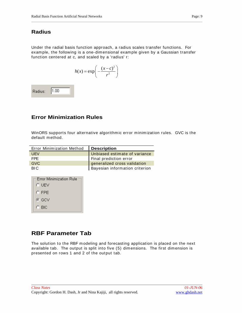
Under the radial basis function approach, a radius scales transfer functions. For example, the following is a one-dimensional example given by a Gaussian transfer function centered at c, and scaled by a 'radius' r:

2

2

( )( ) exp

x ch x

r

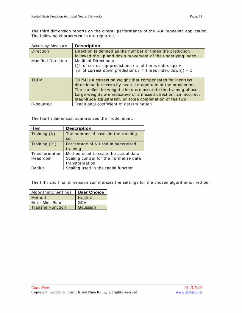
Error Minimization Rules

WinORS supports four alternative algorithmic error minimization rules. GVC is the default method.

Error Minimization Method Description UEV Unbiased estimate of variance FPE Final prediction error GVC generalized cross validation BIC Bayesian information criterion

RBF Parameter Tab

The solution to the RBF modeling and forecasting application is placed on the next available tab. The output is split into five (5) dimensions. The first dimension is presented on rows 1 and 2 of the output tab.




Dimensions

Dimension 1 begins on row 1 indicates the model number. Row 2 restates the name of the target variable.

Descriptor Model Characteristic Blank Model Target Title Entered on the Data

Sheet

The second dimension is displayed from row 4 through row 8. The variables displayed are:

Parameter Description Lambda: The regularization parameter Actual Error: MSE of the training data set prior to

RBF extensions Training Error: MSE of the training data set Validation Error: MSE of the validation set Fitness Error: MSE of the training and validation

sets




The third dimension reports on the overall performance of the RBF modeling application. The following characteristics are reported.

Accuracy Measure Description Direction Direction is defined as the number of times the prediction

followed the up and down movement of the underlying index. Modified Direction Modified Direction =

((# of correct up predictions / # of times index up) + (# of correct down predictions / # times index down)) – 1

TDPM TDPM is a correction weight that compensates for incorrect directional forecasts by overall magnitude of the movement. The smaller the weight, the more accurate the training phase. Large weights are indicative of a missed direction, an incorrect magnitude adjustment, or some combination of the two.

R-squared Traditional coefficient of determination

The fourth dimension summarizes the model input.

Item Description Training (N) The number of cases in the training

set Training (%) Percentage of N used in supervised

training Transformation

Method used to scale the actual data Headroom Scaling control for the normalize data

transformation Radius Scaling used in the radial function

The fifth and final dimension summarizes the settings for the chosen algorithmic method:

Algorithmic Settings User Choice Method Kajiji-4 Error Min. Rule GCV Transfer Function Gaussian




RBF Predicted Tab

The RBF predicted tab presents the actual and predicted data for the current model. This data tab forms the foundation of the RBF diagnostic graphs.




RBF Weights

The final weights determined by the training phase of the solution are presented on this tab.




RBF Diagnostic Graphs

The WinORS Charts menu supports pre-programmed graphs for many of the WinORS applications. These graphs are referred to as diagnostic graphs. Choose the menu tree: /CDR to display the RBF predictive ability graph.




Zoom- In and Zoom-Out

For long time series, it is often useful to zoom-in and inspect a smaller part of the modeled relationship. To zoom the WinoORS graph, follow these steps:

1. Place the mouse in the graph window. For example, place it about 3/4 from the right edge of the displayed graph.

2. Press and hold the left mouse button. 3. Move the mouse to the right. 4. Release the mouse button to see the zoomed image. 5. Repeating this action with a left-oriented movement will zoom-out the graph.




Data Transformations: Standardized

WinORS supports two alternative methods of standardizing the data input values. These are defined below as standardized method 1 and standardized method 2.

Standardized Method 1

Method 1 is the well-known approach to creating a standardized value: ( )X

Z .

Standardized Method 2

This method is invoked by subtracting the mean from all the data observations and multiplying by the square root of the inverse of the covariance matrix ( ). The square root can be found since the covariance matrix is symmetric and can be diagonalized. This method essentially performs a coordinate transformation of a distribution to a different one where the new distribution has zero mean and the covariance matrix is the identity matrix. Let X be any random vector. The whitening transform of X

Y is given

by: 1/ 2 ( )TY X , where is the mean vector.




Data Transformations: Normalized

Using alternative data transformation functions can produce noticeably different RBF solutions. WinORS supports four data normalizing methods. The following notation is common to the four supported techniques.

Term Definition

DL

Lower scaling value

DU

Upper scaling value

Dmin

Minimum data value

Dmax

Maximum data value

SL Lower headroom (%)

SU Upper headroom (%)

Where the values DL and DU are defined by for all supported normalized transformations:

DL = D

min – ((D

max – D

min) x SL) / 100)

DU = D

max + ((D

max – D

min) x SU) / 100),

Normalized Method 1

This approach computes a normalized data input value (DV) from the actual data point (D) by:

DV = (D – D

L) / (D

U – D

L).

The upper and lower headroom percent, SL and SU, are set separately during the model-building exercise. Each is controlled by an associated spin control on the dialog form.

Normalized Method 2

Data is scaled to a range required by the input neurons of the RBF ANN. Contemporary settings for the range are -1 to 1, or, 0 to 1. As with normalized method 1, both DL and

DU are computed as shown above. The data range over which the network models the

transformed data (DV) is based on the settings for SL and SU. Specifically, the transformation is:

DV = S

L + (S

U - S

L)*(D- D

L)/( D

U - D

L).

The values for SL and SU are controlled by the use of an associated spin control on the

dialog form.




Data Transformation: Uniform Data Method

The uniform method is designed to increase data uniformity during the process of scaling the input data into an appropriate range for neural network analytics. The method utilizes a statistical measure of central tendency and variance to remove outliers and spread out the distribution of the data. First, the mean and standard deviation for the input data associated with each input are determined. Next, SL is then set to the mean minus some number of standard deviations. The number of standard deviations is set by a spin control on the dialog box. Similarly, SU is set to the mean plus two standard

deviations. By way of example, assume that the calculated mean and standard deviation are 50 and 3, respectively. Further, assume the user arbitrarily scales with a standard deviation of 2. Under these settings the SL value would be 44, or (50-2*3). The SU value is 56, or (50+2*3). Finally, all data values less than SLare set to SL and all data

values greater than SU are set to SU. The linear scaling described under Method 2 is

applied to the truncated data. By clipping off the ends of the distribution this way, outliers are removed, causing data to be more uniformly distributed.

The RBF Dialog Form and Sample Output

Below is a sample view of the RBF dialog form. The view depicted shows the input for normalized method 2.




The RBF Parameters tab - Normalize Method 1

Subsequent solutions are appended to the next available column on the RBF Parameter tab. This is the case for the other two solution tabs as well (RBF Predicted and RBF Weights). All output descriptions as are previously reviewed.

RBF Diagnostic Graph - Normalize Method 1

For completeness and comparative purposes (against the standardized data transformation), the RBF diagnostic graph of actual and predicted values is displayed below.




Simulation

One of the difficult modeling issues all neural network researchers must confront is to determine how much of the data series should be used to train the network. WinORS provides a simulation option that focuses directly on this issue. The purpose of the simulation option is to locate the settings that produce the smallest network MSE within the simulation range. NOTE: The simulation option is only available when one of the following data transformation methods is invoked: normalized method 1; normalized method 2; and, uniform.

1. Begin by selecting the data transformation method, the RBF Method, Error Minimization Rule, and the desired Transfer Function.

2. Click the checkbox next to the Simulate option. 3. Use the spin control to set the observation from which to start the simulation

procedure. The simulation begins from this value up to the last training observation (in the graphic, simulation will start at observation 100 and continue up to 213).

4. Click Execute to start the simulation and produce an answer.




Simulation Warning

WARNING! Simulation is a time-intensive procedure. For example, in the case of the settings as displayed above, for each data row in the simulation range six RBF solutions are computed -- one for headroom percent beginning at zero percent up to five percent. For the exhibit above where simulation is set for data observations 100 to 213 (114 observation rows), a total of 684 RBF solutions will be computed. While the solution time for each individual execution of the RBF algorithm will depend on a number of factors, assume that one solution requires 5 seconds to compute (including screen updates). Under these assumptions the simulation would require approximately 57 minutes to complete all operations (3,420 seconds). The final solution will report, the observation number and headroom percent combination that produced the smallest model MSE. Fortunately, the simulation option is only needed once (per selected transformation method).

Simulation Results

The simulation results are summarized in two alternative formats; one graphical and one tabular on the spreadsheet tab 'RBF Simulate'.

Simulation: Graphical Results

A graphical result of the simulation effort is presented below. This chart is produced by using the menu tree: CHARTS/DIAGNOSTICS/RADIAL BASIS FUNCTION… Choose the Simulation Results option on the pick list.

A review of the 3-D chart shows that the smallest MSE measures are produced around observation 180 with a low headroom % value. The 'best' solution is found exactly on the 'RBF Simulate' tab.




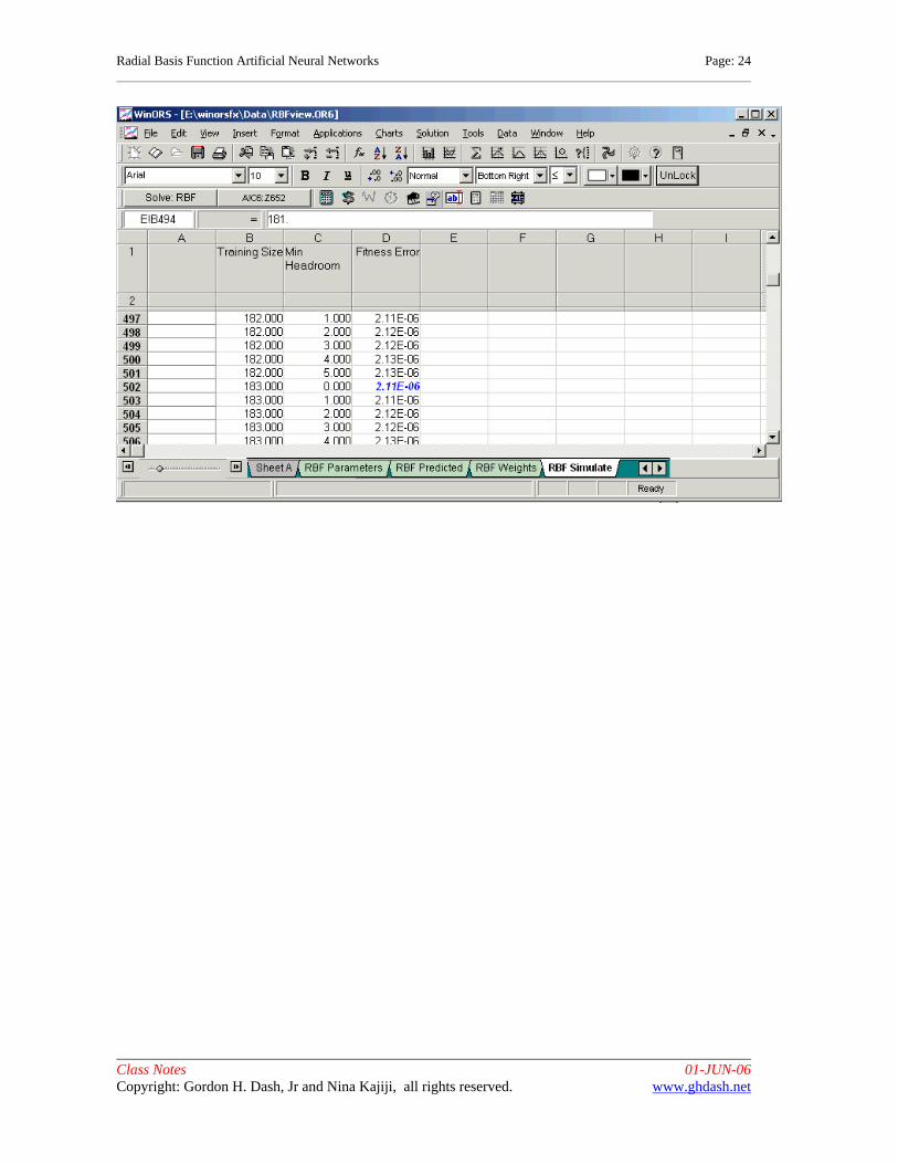
Simulation Results: Tabular

The Simulate Tab presents three columns for your review. First, the number of observations used in the current simulation is presented under the column titles 'Training Size'. In the specific case of the simulation discussed in this document, the next column focuses on the 'Headroom' simulation parameter. Finally, the MSE model fitness error is presented in column D.

The lowest fitness MSE value is highlighted in the color blue. In the case of the scripted analysis presented in this chapter, the lowest fitness MSE occurs with when solving a model with 183 training rows and a minimum headroom of zero percent (0.0%).


Radial Basis Function Artificial Neural Networks · Radial Basis Function Artificial Neural...

Documents

Transcript of Radial Basis Function Artificial Neural Networks · Radial Basis Function Artificial Neural...