RADARGRAMMETRY ON THREE PLANETS

RADARGRAMMETRY ON THREE PLANETS

R.L. Kirk and E. Howington-Kraus

Astrogeology Program, U.S. Geological Survey, 2255 N. Gemini Dr., Flagstaff, Arizona 86001 USA - [email protected]

Commission IV, WG IV/7

KEY WORDS: Spaceborne Remote Sensing, Synthetic Aperture Radar (SAR), Radargrammetry, Visualization, Geology,

Topographic Maps, Adjustment, Sensor Models ABSTRACT: Synthetic Aperture Radar (SAR) can provide useful images in situations where passive optical imaging cannot, either because the microwaves used can penetrate atmospheric clouds, because active imaging can "see in the dark," or both. We have participated in the NASA Magellan mission to Venus in the 1990s and the current NASA-ESA Cassini-Huygens mission to Saturn and Titan, which have used SAR to see through the clouds of Venus and Titan, respectively, and have developed software and techniques for the production of digital topographic models (DTMs) from radar stereopairs. We are currently preparing for similar radargrammetric analysis of data from the Mini-RF instrument to be carried to the Moon on both the ISRO Chandrayaan-1 and NASA Lunar Reconnaissance Orbiter (LRO) missions later in 2008. These instruments are intended to image the permanently shadowed areas at the lunar poles and even see below the surface to detect possible water ice deposits. In this paper, we describe our approach to radargrammetric topographic mapping, based on the use of the USGS ISIS software system to ingest and prepare data, and the commercial stereoanalysis software SOCET SET (® BAE Systems), augmented with custom sensor models we have implemented, for DTM production and editing. We describe the commonalities and differences between the various data sets, and some of the lessons learned, both radargrammetric and geoscientific.

1. INTRODUCTION

Synthetic Aperture Radar (SAR) can provide useful images in situations where passive optical imaging cannot, either because the microwaves used can penetrate atmospheric clouds and even peek beneath the solid surface, because active imaging can "see in the dark," or both. Past planetary applications of SAR have exploited its cloud-penetrating abilities, as part of the Magellan mission to Venus and the Cassini/Huygens investigation of Saturn’s giant satellite Titan. Beginning in 2008, closely related instruments on two lunar orbiters will use polarimetric radar to image the permanently shadowed areas of the lunar poles and search for subsurface ice deposits. We have participated in data analysis for all four of these planetary imaging radars, focusing on the generation of map products. We describe the techniques for radargrammetry (precisely analogous to photogrammetric analysis of passive optical images, but based on the different geometric principles by which radar images are formed) that we have developed and applied to these data sets. This work encompasses both the production of controlled image products by bundle adjustment (solution for improved image orientation parameters and ground coordinates of features, based on measurements of corresponding features in the images) and the production of digital topographic models (DTMs) by automated and/or manual identification of dense sets of image correspondences. Our approach to radargrammetry is to make synergistic use of digital cartography software written in-house at the USGS with a commercial softcopy stereo system.

2. VENUS

2.1 Magellan Mission and Data

Venus is Earth’s sister planet in terms of size and position in the solar system, but hardly an identical twin. The surface is hidden by a dense carbon dioxide atmosphere with cloud decks of sulfuric acid, under which the pressure at the surface is more than 90 atmospheres and the temperature is 735 K. The Magellan spacecraft entered Venus orbit in 1990 with a radar imager/altimeter as its only instrument and high resolution global mapping of the surface as its primary goal. By 1992, Magellan had made three complete cycles of polar orbits, each cycle covering the full range of longitudes. During this time the spacecraft obtained SAR images in S band (12.6 cm λ) covering >96% of the planet at a ground sample distance of 75 m/pixel (Saunders et al., 1992). Images taken with a decreased look angle from vertical, primarily during Cycle 3, provide stereo coverage of 17% of the planet when combined with images with same-side illumination from earlier in the mission (primarily Cycle 1). The stereo geometry of these images is extremely favorable, allowing elevation measurements with an estimated vertical precision (EP) of ~10 m (Leberl et al., 1992). Opposite-side coverage was obtained over a greater area with even stronger stereo geometry, and can be useful in mapping areas of low relief such as the lowland plains. Magellan also obtained radar altimetry data at a horizontal resolution of 10x25 km, but photogrammetric analysis of the stereoimagery can yield topographic maps with a horizontal resolution more than an order of magnitude superior to that of the altimeter. The SAR data from each Magellan orbit were recorded as an F-BIDR (Full-resolution Basic Image Data Record), a ~20x17,000 km strip with 75 m pixel spacing. The BIDR data set was not distributed widely, but was archived on magnetic tape and later on CD-ROMs, with copies at the NASA Planetary Data System

973

The International Archives of the Photogrammetry, Remote Sensing and Spatial Information Sciences. Vol. XXXVII. Part B4. Beijing 2008

(PDS) Geosciences node and at the USGS in Flagstaff, Arizona. For ease of use, mosaics of BIDRs with various scales and formats covering areas ranging from 5°x5° to 120°x120° were made both by the Magellan mission and, later, by the USGS (Batson et al., 1994). The mosaic series (known as MIDRs and FMAPs, respectively) have received wide distribution though the PDS and are available online (http://pds-geosciences.wustl. edu/missions/magellan/index.htm, ftp://pdsimage2.wr.usgs.gov/ cdroms/magellan/) Both the BIDRs and the various mosaics were prepared in Sinusoidal projection for most of Venus, with additional projections used to represent the poles. 2.2 Radargrammetry Implementation

Numerous approaches to radargrammetric processing of the Magellan images have been proposed (e.g., Hensley and Schafer, 1994; Herrick and Sharpton, 2000). Although the USGS briefly considered using an analytic stereoplotter to work with hard copies of Magellan BIDRs (Wu et al., 1987), the large volume (30 GBytes) of same-side stereo data makes a digital or “softcopy” approach desirable if not essential. After working with two such systems, the VEXCEL Magellan Stereo Toolkit (MST; Leberl et al., 1992; Curlander and Maurice, 1993), and the SAIC Digital SAR Workstation-Venus (DSW-V; Wu and Howington-Kraus, 1994) we set out to develop a processing capability that would combine the best features of each, the automated image-matching capability of the MST and the geometrically rigorous sensor model of the DSW-V. To do so, we made use of both the USGS digital cartography system ISIS (Eliason, 1997; Gaddis et al., 1997; Torson and Becker, 1997; see also http://isis.astrogeology .usgs.gov), and the commercial digital photogrammetric software SOCET SET (® BAE Systems) (Miller and Walker, 1993; 1995). We use ISIS to ingest the raw images, prepare them for use (e.g., by decompression, radiometric calibration, geometric distortion correction, as needed for a particular sensor), and export them and their a priori orientation metadata in formats that can be ingested by SOCET SET. SOCET SET then provides tools for bundle adjustment to improve the geodetic control of the images, production of digital terrain models (DTMs) by means of flexible and continuously evolving algorithms for automatic image matching (Zhang and Miller, 1997; Zhang, 2006), display of the images and overlaid DTM data on a stereoscopic monitor for interactive quality control and editing with point, line, and area tools, and production of orthoimages and orthomosaics. We normally export the DTMs and orthoimages back into ISIS for final processing and analysis. This workflow draws on the strengths of both systems (rapid in-house adaptation to new planetary missions for ISIS; rigorous stereogrammetric calculations and 3D display and user input with special hardware in SOCET SET) and forms the basis for our processing of numerous types of optical images from lander cameras (Kirk et al., 1999) to orbit (Kirk et al., 2008a). It is also the basis of our approach to processing SAR data from multiple missions described here. The main difference is that the three “generic” sensor models for different camera types (frame, pushbroom, or panoramic) that are provided with SOCET SET suffice to process the full variety of optical images we have encountered so far. In contrast, each of the radar systems described here has unique characteristics that require the development of a separate sensor model. Although the geometry of SAR image formation is the same in each case, differences in how the data have been projected, combined, and catalogued make it necessary to handle each case individually.

Sensor Model. Mathematically, a sensor model is a function that specifies the transformation between image space (lines, samples) and object or ground coordinates (latitude, longitude, elevation). As implemented in software, a sensor model must also include “bookkeeping” functions to obtain all the information needed to carry out the mathematical transfor-mation and to communicate with the rest of its software environment. The Developers’ Toolkit (DevKit) makes it relatively straightforward to implement new sensor models as “plug ins” to extend the native capabilities of SOCET SET. Our goal in creating a SOCET sensor model for the Magellan SAR (Howington-Kraus et al., 2000) was to make it both physically rigorous and flexible enough to work with all types of Magellan data. The variety of data formats, including multiple types of mosaics as well as single orbit strips, is only one obstacle to working with the Magellan images. This can be handled by defining a Magellan data set for use in SOCET SET as a collection of one or more BIDR strips in Sinusoidal projection, with no restrictions on scale, extent, or center longitude. An additional complication arises because all of the images have been map-projected based on whatever spacecraft trajectory data were available at the time of processing and partially orthorectified based on a low-resolution, pre-Magellan model of Venus’s topography. Our sensor model, based on the one we helped develop for the DSW-V, deals with this processing by using a database containing metadata obtained partly from the mosaic being used and partly from the BIDRs in that mosaic. Specifically, for a given ground point, the sensor model first determines which orbit strip (BIDR) the ground point is contained in, and then which radar burst from that BIDR, by comparing the lat-lon coordinates to strip and burst outlines in the database. Once the radar burst is identified, the burst resampling coefficients and spacecraft position and velocity at the time of observation are obtained from the database. Next, the spacecraft position and velocity are used to calculate the range and Doppler coordinates at which the ground point would be observed. This is the physical process of image formation that we must model, and, unlike the approximate rectification that was done in the original processing, it can incorporate adjustments to the spacecraft trajectory. In this way, we allow for bundle-adjustment of the BIDR strips to improve the positional accuracy of the resulting DTM, even when using images that have been combined in an uncontrolled mosaic. The geometric range just calculated is next corrected for atmospheric refraction. Finally, the resampling coefficients associated with the burst are applied to the range and Doppler coordinates to determine the image coordinates at which this range and Doppler point would have been put into the image. Procedures. Topographic mapping with Magellan data begins with ingestion of the BIDR, MIDR, or FMAP images into ISIS. The full-resolution FMAP mosaics can be used for most DTM production, but in potential problem areas within a mosaic, where pixels are lost at F-BIDR seams, it is necessary to collect DTMs from the unmosaicked F-BIDRs. The BIDRs are also essential if strip-to-strip ties are to be collected for bundle adjustment, and they must be read in the first time a new area is mapped, because they contain the auxiliary data needed to populate the database described above. Only the image data for the latitudes being mapped needs to be retained from the pole-to-pole BIDR strips. Information about the spacecraft position and velocity can be taken either from the BIDR headers or from separate NAIF SPICE kernels (Acton, 1999; data are available from ftp://naif.jpl.nasa.gov/pub/naif/MGN/kernels/), letting us

974


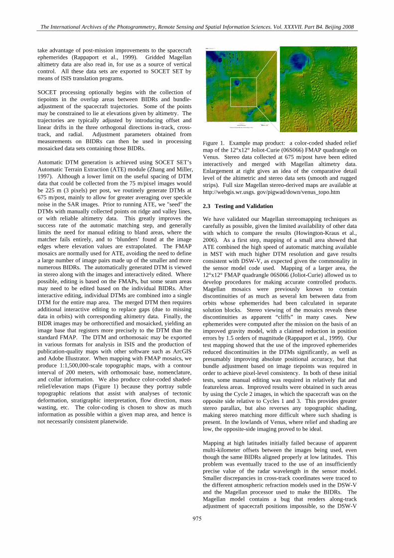
take advantage of post-mission improvements to the spacecraft ephemerides (Rappaport et al., 1999). Gridded Magellan altimetry data are also read in, for use as a source of vertical control. All these data sets are exported to SOCET SET by means of ISIS translation programs. SOCET processing optionally begins with the collection of tiepoints in the overlap areas between BIDRs and bundle-adjustment of the spacecraft trajectories. Some of the points may be constrained to lie at elevations given by altimetry. The trajectories are typically adjusted by introducing offset and linear drifts in the three orthogonal directions in-track, cross-track, and radial. Adjustment parameters obtained from measurements on BIDRs can then be used in processing mosaicked data sets containing those BIDRs. Automatic DTM generation is achieved using SOCET SET’s Automatic Terrain Extraction (ATE) module (Zhang and Miller, 1997). Although a lower limit on the useful spacing of DTM data that could be collected from the 75 m/pixel images would be 225 m (3 pixels) per post, we routinely generate DTMs at 675 m/post, mainly to allow for greater averaging over speckle noise in the SAR images. Prior to running ATE, we "seed" the DTMs with manually collected points on ridge and valley lines, or with reliable altimetry data. This greatly improves the success rate of the automatic matching step, and generally limits the need for manual editing to bland areas, where the matcher fails entirely, and to ‘blunders’ found at the image edges where elevation values are extrapolated. The FMAP mosaics are normally used for ATE, avoiding the need to define a large number of image pairs made up of the smaller and more numerous BIDRs. The automatically generated DTM is viewed in stereo along with the images and interactively edited. Where possible, editing is based on the FMAPs, but some seam areas may need to be edited based on the individual BIDRs. After interactive editing, individual DTMs are combined into a single DTM for the entire map area. The merged DTM then requires additional interactive editing to replace gaps (due to missing data in orbits) with corresponding altimetry data. Finally, the BIDR images may be orthorectified and mosaicked, yielding an image base that registers more precisely to the DTM than the standard FMAP. The DTM and orthomosaic may be exported in various formats for analysis in ISIS and the production of publication-quality maps with other software such as ArcGIS and Adobe Illustrator. When mapping with FMAP mosaics, we produce 1:1,500,000-scale topographic maps, with a contour interval of 200 meters, with orthomosaic base, nomenclature, and collar information. We also produce color-coded shaded-relief/elevation maps (Figure 1) because they portray subtle topographic relations that assist with analyses of tectonic deformation, stratigraphic interpretation, flow direction, mass wasting, etc. The color-coding is chosen to show as much information as possible within a given map area, and hence is not necessarily consistent planetwide.

Figure 1. Example map product: a color-coded shaded relief map of the 12°x12° Joliot-Curie (06S066) FMAP quadrangle on Venus. Stereo data collected at 675 m/post have been edited interactively and merged with Magellan altimetry data. Enlargement at right gives an idea of the comparative detail level of the altimetric and stereo data sets (smooth and rugged strips). Full size Magellan stereo-derived maps are available at http://webgis.wr.usgs. gov/pigwad/down/venus_topo.htm 2.3 Testing and Validation

We have validated our Magellan stereomapping techniques as carefully as possible, given the limited availability of other data with which to compare the results (Howington-Kraus et al., 2006). As a first step, mapping of a small area showed that ATE combined the high speed of automatic matching available in MST with much higher DTM resolution and gave results consistent with DSW-V, as expected given the commonality in the sensor model code used. Mapping of a larger area, the 12°x12° FMAP quadrangle 06S066 (Joliot-Curie) allowed us to develop procedures for making accurate controlled products. Magellan mosaics were previously known to contain discontinuities of as much as several km between data from orbits whose ephemerides had been calculated in separate solution blocks. Stereo viewing of the mosaics reveals these discontinuities as apparent “cliffs” in many cases. New ephemerides were computed after the mission on the basis of an improved gravity model, with a claimed reduction in position errors by 1.5 orders of magnitude (Rappaport et al., 1999). Our test mapping showed that the use of the improved ephemerides reduced discontinuities in the DTMs significantly, as well as presumably improving absolute positional accuracy, but that bundle adjustment based on image tiepoints was required in order to achieve pixel-level consistency. In both of these initial tests, some manual editing was required in relatively flat and featureless areas. Improved results were obtained in such areas by using the Cycle 2 images, in which the spacecraft was on the opposite side relative to Cycles 1 and 3. This provides greater stereo parallax, but also reverses any topographic shading, making stereo matching more difficult where such shading is present. In the lowlands of Venus, where relief and shading are low, the opposite-side imaging proved to be ideal. Mapping at high latitudes initially failed because of apparent multi-kilometer offsets between the images being used, even though the same BIDRs aligned properly at low latitudes. This problem was eventually traced to the use of an insufficiently precise value of the radar wavelength in the sensor model. Smaller discrepancies in cross-track coordinates were traced to the different atmospheric refraction models used in the DSW-V and the Magellan processor used to make the BIDRs. The Magellan model contains a bug that renders along-track adjustment of spacecraft positions impossible, so the DSW-V

975


model was adopted. Mapping to the east of the Joliot-Curie quadrangle revealed that the quality of the Cycle 3 images declined dramatically toward the end of the cycle in terms of both signal-to-noise ratio and data dropouts, increasing the need for interactive editing by a factor of several. A particular concern of the geologists interested in using Magellan stereo DTMs was whether artifacts could occur at high-contrast boundaries, either directly by effects on the SAR images or as a result of the errors that such boundaries were known to induce in the altimetry used for vertical control. We addressed these issues by test mapping of a 10°x3° region in the rugged highlands of Ovda Regio containing sharp boundaries between high and low radar backscatter. These boundaries are caused by a temperature-dependent change in the equilibrium mineral phases on the surface, so they are expected to form at nearly constant elevation. The images clearly show the surface to be smoothly sloping near the boundaries, but the altimetry contains artifactual “pits” as deep as 3 km. We found, as expected, that our smooth (linear with time) adjustment to the spacecraft ephemerides did not allow the stereo DTM surface to deform to follow altimetry artifacts. Vertical control points placed in the “pits” were readily identified as outliers, and the stereo DTM indicated highly consistent elevations along the contrast boundary, with variations of ~200 m locally, compared to ~500 m variation previously estimated by mapping with uncontrolled images in MST (Arvidson et al., 1994). The constancy of the transition elevation provides as good a test of the precision of our stereo mapping as is likely to be obtained until a future mission supplies higher resolution data. 2.4 Lessons Learned

Overall, our Magellan experience showed that digital stereo-grammetric processing techniques, including automatic image matching, could be applied successfully to planetary SAR data, and that a custom sensor model could be used to bundle adjust and work with images that had already been map projected and even mosaicked. Our tests showed the utility of a “seed” DTM for automatic matching and the value of opposite-side radar stereopairs for mapping areas of subtle relief, and suggested what may be a general rule, that accurate mapping requires both the best available reconstructed ephemerides and further bundle adjustment based on image tiepoints. Finally, we learned not to underestimate the additional complications and difficulties that arise in the mapping of each new area of Venus.

3. TITAN

3.1 Cassini Mission and Data

The Cassini-Huygens mission consists of the NASA Cassini spacecraft, which went into orbit around Saturn in 2004, and the ESA Huygens probe carried by Cassini, which landed on the giant satellite Titan in 2005. Investigation of Titan, which is larger than the planet Mercury and wrapped in a smoggy nitrogen atmosphere four times denser than Earth’s, is a major objective of the Cassini instruments as well as the sole goal of Huygens. Prior investigations of the organic chemistry of Titan’s atmosphere raised the strong possibility of reservoirs of liquid methane and ethane on the body’s surface, where they might be expected to form lakes and even participate in an exotic equivalent of Earth’s hydrologic cycle. The RADAR instrument (Elachi et al., 2004) uses Ku band (2.17 cm λ) microwaves to penetrate the atmospheric clouds and haze, and

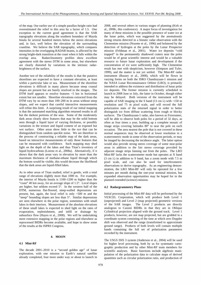
has provided the highest resolution images of Titan's surface apart from very localized coverage from the cameras on Huygens. On selected flybys of Cassini past Titan, the RADAR obtains a SAR image strip 200–500 km wide and as much as 6000 km (130° of arc) in length. So far, approximately 25% of Titan's surface has been imaged, at resolutions from about 0.3 to 1.5 km; a grid spacing of 175 m (1/256°) is used to ensure oversampling of the data. Beginning in late 2006, most new SAR image strips partly overlapped one or more earlier images, and by the end of 2007, more than 20 image overlaps covering more than 1% of Titan in stereo were available (Figure 2). Operating in other modes, the RADAR also provides lower resolution altimetry, scatterometry, and radiometry data. As in the Magellan mission, the image strips are known as BIDRs (Stiles, 2008b) and are made available in map projected form. The pattern of Cassini flybys (Fig. 2) is much less regular than the north-south arrangement of orbit strips on Venus, however, so each BIDR uses an Oblique Cylindrical projection oriented along its individual flyby ground track. Mosaics of multiple BIDRs transformed to a common global map projection are being made, but these are not useful for stereoanalysis because there is no equivalent to the Cycle-1 and Cycle-3 data sets of Magellan. Instead, we use the individual BIDRs and map the overlap areas of pairs of them.

Figure 2. Mosaic of Cassini RADAR image coverage of Titan. Polar Stereographic projections of the northern (left) and southern (right) hemispheres with 10° parallels. Longitude 0° is at the bottom on left, at top on right. Stereo overlaps with same-side illumination and viewing are shown in green, opposite-side in red, and high-angle overlaps in yellow. Total coverage to date is ~25%, total stereo ~1%. 3.2 Methodology

Our approach to radargrammetry with Cassini data closely follows that outlined above for Magellan, in broad outline using ISIS to ingest and prepare the data and SOCET SET with a custom sensor model written by us to perform bundle adjustment, automated matching, and DTM editing. The inputs for mapping are BIDRs in Oblique Cylindrical projection rather than BIDRs, MIDRs, and FMAPs in Sinusoidal projection, but the sensor model follows the same steps of identifying the relevant radar burst for a given ground point, calculating the range-Doppler coordinates of the point for that burst, and then duplicating the transformation of range-Doppler into BIDR pixel coordinates. The Cassini BIDRs must be treated as mosaics, however, because they contain five parallel swaths of data obtained by the five separate beams of the instrument. It is thus necessary to identify first the beam and then the burst whose parameters should be used in sensor model calculations for any given pixel. The small number of BIDRs (tens versus

976


thousands for Magellan) and random rather than north-south orientation made it more convenient to store the beam-and-burst information as a raster map in the same projection as the image, rather than as a tabular database. The needed ancillary data for each burst, including both its footprint boundary and the space-craft position and velocity, are obtained from a binary table known as the SBDR (Stiles, 2008a). A final difference between the Magellan and Cassini processing comes about because there is no pre-Cassini topographic information for Titan. Cassini BIDRs are therefore projected onto a spherical reference surface rather than onto a low-resolution DTM. Because the equations of projection onto a sphere can be expressed analytically, no resampling coefficients are required. Care is needed, however, to use the adjusted spacecraft position and velocity to calculate range-Doppler coordinates from the ground point location, but to use the original position and velocity estimates to calculate map coordinates from range and Doppler, in order to be consistent with the way the BIDRs were generated.

Our approach to processing the Cassini RADAR stereopairs has also been informed by our experience with Magellan. In particular, the practice of “seeding” the automatic matching process with a loose set of surface points selected interactively has once again been shown to reduce the need for final editing. The initial mapping results reported below were obtained without any bundle adjustment, but we expect that as we analyze a larger number of overlap areas, some adjustment will be necessary to achieve consistent results at the sub-kilometer level of precision. 3.3 Results

Evidence about the topography of Titan prior to our beginning radargrammetric mapping with SOCET SET came from a variety of sources, all of which suggested that both local and global relief is low, with elevation variations greater than about 1000 m rare. Radarclinometry (shape-from-shading) initially revealed only a few hundred meters relief in areas where it could be applied (Kirk et al., 2005) though more recent results reach 1500–2000 m for some mountains (Radebaugh et al., 2007). Topographic profiles have been obtained over a limited number of short arcs by operating the RADAR as an altimeter

(Johnson et al., 2007) and over longer arcs by an ingenious method that compares the signal strength from adjacent overlapping beams to determine heights along each SAR image (Stiles et al., 2007). The profiling methods agree well where they have been compared (Gim et al., 2007), and both show relief of a few hundred meters or less. Finally, preliminary estimates of topography from stereo, again indicating relief of hundreds of meters (Kirk et al., 2007) were based on automated image matching by Scott Hensley at JPL and on manual parallax measurements by us, but in either case a simple parallax-height scaling based on the two radar incidence angles was used in lieu of a rigorous sensor model to estimate relative elevation differences. Hensley has since implemented a rigorous Cassini RADAR sensor model for his Magellan-derived matching software (written communication, 2007). Our plans to map the complete set of RADAR overlap areas now that a rigorous sensor model is available for SOCET SET have been delayed somewhat by the discovery of substantial (up to 30 km) positional mismatches between many of the image pairs that would introduce spurious parallax and/or prevent stereo matching altogether. These offsets have been traced to the need for an improved model of Titan’s rotation, and have been reduced to sub-km levels by adjusting the orientation of the spin axis, the rotation rate, and the first derivatives of these parameters (Stiles et al., 2008). The nonsynchronous spin rate, in particular, implies that the ice crust of Titan is decoupled from the deep interior by a subsurface liquid water “ocean” (Lorenz et al., 2008b)—an interesting example of a significant geophysical discovery arising from a routine use of radargrammetry to improve cartographic products. Reprocessing of the complete set of Cassini BIDRs based on the new rotational model will be completed in the late spring or early summer of 2008. Meanwhile, several overlapping images obtained in 2007 February to April were made at the same rotational phase, so that the misregistration caused by using the older rotation model is negligible. Fortunately, the overlap between these images covers one of the most interesting regions of Titan, an area of extensive dark areas interpreted to be lakes and seas (Stofan et al., 2007) near the north pole.

Figure 3. Color-coded topographic map of part of Titan’s north polar “lake country” based on stereoanalysis of RADAR images from flybys T25 and T28. Polar stereographic projection, north approximately at top. Island at right center is Mayda Insula, discussed in text.

Figure 3 shows our topographic model of the overlap between the images from the T25 (2007 February 22) and T28 (2007 April 10) flybys. Both flybys illuminated the area from the south, yielding same-side stereo with vertical precision typically on the order of 100 m for single pixel (175 m) matching error. The procedures for making this DTM were tested by initial mapping of Mayda Insula, a 90x150 km island

centered near 78° N 312° W (Kirk et al., 2008c). Bundle adjustment was not needed for this data set, because cross-stereobase misregistration was less than one pixel, and the unadjusted stereo elevations along the SAR topography profile agreed at the 50–100 m level with the absolute elevations of the latter data set. We note that that this agreement is obtained even where the two incidence angles are similar, at the east end

977


of the map. Our earlier use of a simple parallax-height ratio had overestimated the relief in this area by a factor of 1.5. One exception to the current good agreement is that the SAR topography elevations along the southern boundary of Mayda Insula lie several hundred meters below the stereo elevations and, in fact, well below the elevation of the surrounding coastline. We believe the SAR topography, which compares intensities in the overlapping RADAR beams, is affected by the strong bright-dark transition at the coast when it falls within the overlap area. Radarclinometry profiles show excellent agreement with the stereo DTM in some areas, but elsewhere are clearly distorted by variations in the intrinsic radar-brightness of the surface. Another test of the reliability of the results is that the putative shorelines are expected to have a constant elevation, at least within a particular lake or sea. Measurement of the shoreline elevations is difficult in many places because steep coastal slopes are present but are barely resolved in the images. The DTM itself appears to resolve features ~5 km in horizontal extent but not smaller. Shoreline elevations extracted from the DTM vary by no more than 100–200 m in areas without steep slopes, and we expect that careful interactive measurements will refine this limit. A surprising result of our initial mapping is that the automated matching algorithm returned results in all but the darkest portions of the seas. Some of the moderately dark areas clearly show features that may be the solid bottom seen through a liquid layer of varying thickness, or possibly variations in the texture and liquid content of an exposed but wet surface. Other areas show little to the eye that can be distinguished from random speckle noise. We are therefore in the process of constructing a reliable map of the dark areas, based on interactive measurements of only those features that can be measured with confidence. Such mapping may shed light on the depth of the lakes and thus Titan’s inventory of liquid hydrocarbons (Lorenz et al., 2008a). Alternatively, if it shows that the dark areas vary in elevation by more than the maximum thickness of methane-ethane liquid through which the bottom would be visible, this would decrease the likelihood that the dark areas are liquid-filled lakes. As in other areas of Titan studied, relief is gentle, with a total range of elevations slightly more than 1000 m. For example, the interior of Mayda Insula is 1100–1200 m higher than the “coast” 40 km away, for an average slope of 1.5°. Local slopes are higher, but seldom exceed 5°. In the western half of the DTM, numerous flat-floored, steep-walled depressions are present, but, again, the local relief is only ~500 m and the “steep” bounding slopes are less than 5°. Similar depressions are seen elsewhere in the polar region, sometimes with small lakes in their interiors. Measurement of the absolute elevations of these small lakes is expected to shed light on the rates of evaporation, replenishment, and infill or drainage by subsurface flow (Hayes et al., 2008). We will be undertaking more extensive mapping in the polar regions and elsewhere as reprocessed BIDRs become available, and hope to show some of the results at the ISPRS Congress.

4. MOON

4.1 Mini-RF

The decade 2001–2010 is a “second golden age” of lunar exploration, with one mission to Earth’s natural satellite already completed, four more under way or about to launch in

2008, and several others in various stages of planning (Kirk et al., 2008c, this conference). A major focus of investigation for many of these missions is the possible presence of water ice at the lunar poles, which was suggested by the anomalously strong returns detected in a bistatic radar observation with the Clementine mission (Nozette et al., 1996) and bolstered by the detection of hydrogen at the poles by the Lunar Prospector mission (Feldman et al., 2001). Water ice deposits “cold trapped” in the permanently shadowed craters near the poles would be of great scientific interest and would be a valuable resource to future lunar exploration and development if the concentration of ice were sufficiently high. The Clementine result has met with skepticism, however (Simpson and Tyler, 1999), and the matter is not yet settled. The Mini-RF radar instrument (Bussey et al., 2008), which will be flown in varying forms on both the ISRO Chandrayaan-1 mission and the NASA Lunar Reconnaissance Orbiter (LRO), is primarily intended to address the existence and distribution of lunar polar ice deposits. The former mission is currently scheduled to launch in 2008 June or July, the latter in October, though either may be delayed. Both versions of the instrument will be capable of SAR imaging in the S band (13 cm λ) with ~150 m resolution and 75 m pixel scale, and will record the full polarization state of the returned signal in order to better distinguish ice from diffuse scattering from rough or blocky surfaces. The Chandrayaan-1 radar, also known as Forerunner, will be able to observe both poles for a period of 32 days, as often as four times a year, building up a complete mosaic of image strips covering latitudes 80° to near the pole on each occasion. The area nearest the pole that is not covered in these normal sequences may be observed at lower resolution in a scatterometric mode in some of the observation periods, or may be imaged by decreasing the incidence angle. The latter option would also provide strong stereo coverage of some near-polar areas in addition to the fair stereo coverage provided by adjacent image strips fanning out from the poles. The LRO Mini-RF lacks the scatterometer mode but operates at X band (3 cm λ) in addition to S band, has a zoom mode with 7.5 m pixel scale, and can also be used for interferometric observations to derive topography. As an engineering demon-stration, the LRO Mini-RF will only be operated for a few minutes per month during the one-year nominal mission, but expanded observation opportunities may be hoped for in the planned extended (science) mission. 4.2 Radargrammetry Plans

Initial processing of the Mini-RF data will be performed by the VEXCEL Corporation, which will produce both Level 1 (unprojected) and Level 2 (map projected) geometric versions of the SAR images. The Level 2 products are directly analogous to Cassini BIDRs in that they are in Oblique Cylindrical projection aligned with the ground track. Level 1 products, however, are not map projected, but are gridded in a coordinate system consisting of the time at which zero Doppler shift was observed and the range (transformed to approximate ground range). Products of both levels will contain multiple bands containing the full set of polarization parameters recorded by the instrument. The USGS ISIS 3 system (Anderson et al., 2004) will be used for higher level processing, both by us for systematic carto-graphic production and by other Mini-RF team members for scientific analyses. Basic functions include algebraic mani-pulation of the polarization data to calculate maps of derived quantities such as circular polarization ratio, and production of

978


uncontrolled mosaics from the VEXCEL Level 2 files. We are also developing (with the assistance of colleagues at Arizona State University) an ISIS sensor model that will allow Level 1 products to be orthorectified by projection onto a DTM of choice. With further development based on this sensor model, bundle adjustment of Mini-RF Level 1 images in ISIS and the production of controlled mosaics will be possible. Finally, we are developing the software to import Level 1 images into SOCET SET and a SOCET sensor model that will permit bundle adjustment and DTM extraction. The design of the ISIS and SOCET sensor models for Mini-RF is tremendously simplified by the availability of the Level 1 products. After calculating the range-Doppler coordinates of a ground point by the same calculations used for Magellan and Cassini, it is necessary merely to iterate to find the time at which the Doppler shift is zero, then carry out a simple transformation to Level 1 line and sample coordinates. In particular, there is no need for a database or bit map to determine what radar burst observed the given ground point. We expect confidently to be able to make controlled image mosaics by performing bundle adjustments in ISIS and/or SOCET SET, and to make stereo DTMs with useful post spacing on the order of 200–300 m. Although such products may ultimately be superseded by the very accurate, high density laser altimetry data expected from LRO and several of the other missions, they may provide the best interim topographic information about polar regions hidden from the sun and from Earth-based radar mapping.

REFERENCES

Acton, C.H., 1999. SPICE products available to the planetary science community. Lunar Planet. Sci., XXX, Abstract #1233, Lunar and Planetary Institute, Houston (CD-ROM). Anderson, J.A., Sides, S.C., Soltesz, D.L., Sucharski, T.L., and Becker K.J., 2004. Modernization of the Integrated Software for Imagers and Spectrometers. Lunar Planet. Sci., XXXV, Abstract #2039, Lunar and Planetary Institute, Houston (CD-ROM). Arvidson, R.E., et al., 1994. Microwave signatures and surface properties of Ovda Regio and surroundings, Venus, Icarus, 112, pp. 171-186. Batson, R.M., Kirk, R.L., Edwards, K.F., and Morgan, H.F., 1994. Venus cartography. J. Geophys. Res. 99, pp. 21,173–21,182. Bussey, D.B., Spudis, P.D., Nozette, S., Lichtenberg, C.L., Raney, R.K., Marinelli, W., and Winters, H.L., 2008. Mini-RF: Imaging radars for exploring the lunar poles. Lunar Planet. Sci., XXXIX, Abstract #2389, Lunar and Planetary Institute, Houston (CD-ROM). Curlander, J., and Maurice, K., 1993. Magellan Stereo Toolkit User Manual. VEXCEL Corporation (unpublished). Elachi, C. et al., 2004. RADAR: The Cassini Titan Radar Mapper. Space Sci. Rev., 115, p. 71. Eliason, E., 1997. Production of digital image models using the ISIS system. Lunar Planet. Sci., XXVIII, pp. 331–332. Feldman, W.C., et al., 2001. Evidence for water ice near the lunar poles. J. Geophys. Res., 106(E10), pp. 23,231–23,252.

Gaddis, L.R., Anderson, J., Becker, K., Becker, T., Cook, D., Edwards, K., Eliason, E., Hare, T., Kieffer, H., Lee, E.M., Mathews, J., Soderblom, L, Sucharski, T., and Torson, J., 1997. An overview of the Integrated Software for Imaging Spectrometers (ISIS). Lunar Planet. Sci., XXVIII, pp. 387–388. Gim, Y., et al., 2007. Titan topography: A comparison between Cassini altimeter and SAR imaging from two Titan flybys. Eos Trans. AGU, 88(52), Fall Meet. Suppl., Abstract P23B-1351. Hayes, A., et al., 2008. Hydrocarbon lakes on Titan: Distribution and interaction with a porous regolith. Geophys. Res. Lett., in press. Hensley, S., and Schafer, S., 1994. Automatic DEM generation using Magellan stereo data. IGARSS 94, 3, pp. 1470–1472. Herrick, R., and Sharpton, V.I., 2000. Implications from stereo-derived topography of Venusian impact craters. J. Geophys. Res., 106(E6), pp. 20,245–20,262. Howington-Kraus, E., Kirk, R., Galuszka, D., Hare, T., and Redding, B., 2000. Rigorous sensor model for topographic mapping of Venus using Magellan radar stereoimagery. Lunar Planet. Sci., XXXI, Abstract #2061, Lunar and Planetary Institute, Houston (CD-ROM). Johnson, W.T.K. et al., 2007. Cassini RADAR altimeter observations of Titan. Workshop on Ices, Oceans, and Fire, LPI Contribution 1357, pp. 70–71. Kirk, R. L., et al., 1999. Digital photogrammetric analysis of the IMP camera images: Mapping the Mars Pathfinder landing site in three dimensions. J. Geophys. Res., 104(E4), p. 8868–8888. Kirk, R.L., et al., 2008a. Ultrahigh resolution topographic mapping of Mars with MRO HiRISE stereo images: Meter-scale slopes of candidate Phoenix landing sites. J. Geophys. Res., in press. Kirk, R.L., Archinal, B.A., Gaddis, L.R., and Rosiek, M.R., 2008b. Cartography for lunar exploration: 2008 status and mission plans. Int. Arch. Photogramm. Remote Sens. Spatial Info. Sci., XXXVIII(4), this conference. Kirk, R.L., Callahan, P., Seu, R., Lorenz, R. D., Paganelli, F., Lopes, R., Elachi, C., and the Cassini RADAR Team, 2005. RADAR Reveals Titan Topography. Lunar Planet. Sci., XXXVI, Abstract #2227, Lunar and Planetary Institute, Houston (CD-ROM). Kirk, R.L., Howington-Kraus, E., Mitchell, K.L., Hensley, S., Stiles, B.W., and the Cassini RADAR Team, 2007, First stereoscopic radar images of Titan, Lunar Planet. Sci., XXXVIII, Abstract #1427, Lunar and Planetary Institute, Houston (CD-ROM). Kirk, R.L., Howington-Kraus, E., Stiles, B.W., Hensley, S., and the Cassini RADAR Team, 2008c, Digital topographic models of Titan produced by radar stereogrammetry with a rigorous sensor model, Lunar Planet. Sci., XXXIX, Abstract #2320, Lunar and Planetary Institute, Houston (CD-ROM).

979


Leberl, F.W., Thomas, J.K., and Maurice, K.E., 1992. Initial results from the Magellan Stereo Experiment. J. Geophys. Res., 97(E8), pp. 13,675–13,689. Lorenz, R. D., et al., 2008a. Titan’s Inventory of Organic Surface Materials. Geophys. Res. Lett., 15, CiteID L02206, doi:10.1029/ 2007GL032118. Lorenz, R.D., Stiles, B., Kirk, R.L., Allison, M., Persi del Marmo, P., Lunine, J.I., Ostro, S.J., and the Cassini RADAR Team, 2008b. Titan’s changing length of day : An internal water ocean and seasonal variation of atmospheric angular momentum. Science, 319, pp. 1649–1651, doi:10.1126/science. 1151639. Miller, S.B., and Walker, A.S., 1993. Further developments of Leica digital photogrammetric systems by Helava. ACSM/ASPRS Convention and Exposition Technical Papers, 3, pp. 256–263. Miller, S.B., and Walker, A. S., 1995. Die Entwicklung der digitalen photogrammetrischen Systeme von Leica und Helava. Zeitschrift für Photogrammetrie und Fernerkundung, 63(1), pp. 4–16. Nozette, S., Lichtenberg, C.L., Spudis, P., Bonner, R., Ort, W., Malaret, E., Robinson, M., and Shoemaker, E.M., 1996. The Clementine bistatic radar experiment. Science, 274, pp. 1495–1498. Radebaugh, J., Lorenz, R., Kirk, R., Lunine, J., Stofan, E., Lopes, R., Wall, S., and the Cassini RADAR Team, 2007. Mountains on Titan observed by Cassini RADAR. Icarus, 192, 77-92, doi:10.1016/j.icarus.2007.06.020. Rappaport, N.J., Konopliv, A.S., Kucinskas, A.B., and Ford, P.G., 1999. An improved 360 degree and order model of Venus topography. Icarus, 139, pp. 19–31. Saunders, R.S., et al., 1992. Magellan Mission Summary. J. Geophys. Res., 97(E8), pp. 13,067–13,090. Stiles, B., 2008a. Cassini Radar Burst Ordered Data Products SIS. NASA D-27891, Version 2.0, April 18, 208. Stiles, B., 2008b. Cassini Basic Image Data Records SIS. NASA D-27889, Version 2.0, April 22, 208.

Stiles, B.W., Hensley, S., Gim, Y., Kirk, R.L., Zebker, H., Janssen, M.A., and the Cassini RADAR Team, 2007. Estimating Titan surface topography from Cassini Synthetic Aperture RADAR data. Eos Trans. AGU, 88(52), Fall Meet. Suppl., Abstract P23B-1352. Stiles, B., Kirk, R.L., Lorenz, R., Hensley, S., Lee, E., Ostro, S., Gim, Y., Hamilton, G., Johnson, W.T.K., West, R., and the Cassini RADAR Team, 2008. Estimating Titan's spin state from Cassini SAR data. Astronom. J., 135, pp. 1669–1680, doi:10. 1088/0004-6256/135/5/1669. Stofan, E.R., et al., 2007. The lakes of Titan. Nature, 445, doi: 10.1038/nature05438. Torson, J., and K. Becker, 1997. ISIS: A software architecture for processing planetary images. Lunar Planet. Sci., XXVIII, pp. 1443–1444. Simpson, R., and Tyler, L., 1999. Reanalysis of Clementine bistatic radar from the lunar South Pole. J. Geophys. Res., 104(E2), pp. 3845–3862. Wu, S.S.C., and Howington-Kraus, E.A., 1994. Magellan radar data for Venus topographic mapping. Lunar Planet. Sci. XXV, pp. 1519-1520. Wu, S.S.C., Schafer, F.J., and Howington-Kraus, E.A., 1987.A compilation system for Venus radar mission (Magellan). NASA TM-89810, p. 233–236. Zhang, B., 2006. Towards a higher level of automation in softcopy photogrammetry: NGATE and LIDAR processing in SOCET SET®. GeoCue Corporation 2nd Annual Technical Exchange Conference, Nashville, Tennessee, 26–27 September, 32 pp. Zhang, B., and Miller, S., 1997. Adaptive Automatic Terrain Extraction. Proceedings of SPIE, Volume 3072, Integrating Photogrammetric Techniques with Scene Analysis and Machine Vision (edited by D. M. McKeown, J. C. McGlone and O. Jamet). pp. 27-36.

ACKNOWLEDGEMENTS

The research described here has been supported by the NASA Planetary Geology and Geophysics Cartography program, the NASA Magellan, Cassini, and LRO missions, and the NASA element of Chandrayaan-1.

980

RADARGRAMMETRY ON THREE PLANETS

Documents

Transcript of RADARGRAMMETRY ON THREE PLANETS