RADAN 7 for Archaeology, Cemeteries & Forensics · RADAN is a powerful, full-featured platform for...
76
RADAN ® 7 for Archaeology, Cemeteries & Forensics 40 Simon Street • Nashua, NH 03060-3075 USA • www.geophysical.com Geophysical Survey Systems, Inc. Non-Migrated Migrated Migrated Non-Migrated MN43-203 Rev A
Transcript of RADAN 7 for Archaeology, Cemeteries & Forensics · RADAN is a powerful, full-featured platform for...

RADAN® 7 for Archaeology,Cemeteries & Forensics
40 Simon Street • Nashua, NH 03060-3075 USA • www.geophysical.com
Geophysical Survey Systems, Inc.
Non-Migrated
Migrated
Mig
rate
dN
on-
Mig
rate
d
MN43-203 Rev A

PETER LEACH, STAFF ARCHAEOLOGIST Peter joined GSSI in 2016 as the archaeology and forensics application specialist, as well as a member of the training and technical support team. He is a member of the Register of Professional Archaeologists and specializes in terrestrial geophysical methods applied to archaeology, geographic information systems (GIS) analyses, and submerged prehistoric archaeology.
Peter has conducted GPR surveys on four continents as a specialist for academic research teams, and has carried out over 90+ terrestrial geophysical surveys on archaeological sites, in cemeteries, and for forensic searches in the US and Canada.
Prior to joining GSSI, Peter worked as a professional archaeologist in New England and the Mid Atlantic, where he honed his GPR skills “in the trenches.”
Peter is also a doctoral student at the University of Connecticut, with dissertation research focused on precontact archaeological sites submerged by sea-level rise. When not at GSSI Peter spends most of his time reorganizing the feline residents of his computer desk and using his dog as a less-than-ideal footrest.
RECOMMENDED CITATION FORMAT: Leach, Peter. “RADAN 7 for Archaeology, Forensics, and Cemeteries.” Geophysical Survey Systems, Inc. 2019, pp. 70.
Copyright © 2019 Geophysical Survey Systems, Inc. All rights reserved including the right of reproduction in whole or in part in any form Published by Geophysical Survey Systems, Inc. 40 Simon Street Nashua, New Hampshire 03060-3075 USA Printed in the United States SIR, RADAN, PaveScan RDM and UtilityScan are registered trademarks of Geophysical Survey Systems, Inc.
Geophysical Survey Systems, Inc. RADAN® for Archaeology, Cemeteries & Forensics
RADAN 7 FOR ARCHAEOLOGY, FORENSICS, AND CEMETERIES Table of Contents Introduction ...................................................................................................................................... 1 Section 1: Overview of RADAN Processes .................................................................................. 2
1.1. Time Zero ........................................................................................................................ 2 1.2 Range Gain ....................................................................................................................... 2 1.3 Background Removal ....................................................................................................... 3 1.4 FIR and IIR Filters ........................................................................................................... 3 1.5 Migration .......................................................................................................................... 4 1.6 Distance Normalization .................................................................................................... 5 1.7 Horizontal Scaling ............................................................................................................ 5 1.8 Deconvolution .................................................................................................................. 5 1.9 Math Functions................................................................................................................. 6
Section 2: Processing 2D Datasets ................................................................................................ 7 2.1 Time Zero/ Position Correction........................................................................................ 7 2.2 Background Removal ....................................................................................................... 9 2.3 Range Gain ..................................................................................................................... 11 2.4 FIR and IIR .................................................................................................................... 12 2.5 Migration ........................................................................................................................ 21 2.6 Mathematical Functions (Differentiate and Integrate) ................................................... 23 2.7 Gain Restoration ............................................................................................................. 24 2.8 Surface Normalization ................................................................................................... 24 2.9 Deconvolution ................................................................................................................ 26 2.10 Hilbert Transform ......................................................................................................... 27 2.11 Horizontal Scaling ........................................................................................................ 28 2.12 Edit Block..................................................................................................................... 29 2.13 2D Interactive ............................................................................................................... 30 2.14 Using GPS Data with 2D Profiles ................................................................................ 33 2.15 Exporting 2D Data from RADAN ............................................................................... 35 2.16 Google Earth Interface ................................................................................................. 35
Section 3: Recommendations for 3D Datasets ........................................................................... 36 3.1 The Relationship between 2D and 3D Processing and Visualization ............................ 36 3.2 Recommendations for Gridded Field Datasets ............................................................... 36
Section 4: Creating 3D Datasets ................................................................................................. 39 4.1 Creating a Manual 3D File ............................................................................................. 39 4.2 Dealing with Obstacles in Grids (for Manual 3D only) ................................................. 41 4.3 Creating a 3D Batch of Files .......................................................................................... 42 4.4 Creating a Gridded 3D File ............................................................................................ 44 4.5 Creating a Super3D File ................................................................................................. 46 4.6 Adding GPS Data to a 3D Grid (after Data Collection) ................................................. 46
Section 5: Processing Impacts for 3D Datasets ......................................................................... 48
Geophysical Survey Systems, Inc. RADAN® for Archaeology, Cemeteries & Forensics
5.1 Range Gain and 3D Data ................................................................................................ 48 5.2 Time Zero/Position Correction and Near-Surface 3D Data ........................................... 50 5.3 Background Removal and Near-Surface 3D Data ......................................................... 51 5.4 Migration and 3D Data ................................................................................................... 53 5.5 IIR Filter and 3D Data .................................................................................................... 54 5.6 Mathematical Functions and 3D Data ............................................................................ 57
Section 6: Miscellaneous Display Parameters and Export Options for 3D Datasets ............. 60 6.1 Changing Slice Thickness .............................................................................................. 60 6.2 Using Max vs RMS (3D Volume Options Window) ..................................................... 61 6.3 Reducing “Checkerboarding” in Super3D (Tables Pane) .............................................. 62 6.4 Removing the XY Text from the Lower Left Grid Origin ............................................. 63 6.5 Exporting 3D Data from RADAN ................................................................................. 64 6.6 “Rubbersheeting” 3D Data in RADAN ......................................................................... 65
Concluding Remarks ................................................................................................................... 68 Appendix I: GSSI File Header Information .............................................................................. 69 Appendix II: GSSI Antenna Parameters ................................................................................... 70
Geophysical Survey Systems, Inc. RADAN® for Archaeology, Cemeteries & Forensics
1 MN43-203 Rev A
RADAN 7 FOR ARCHAEOLOGY, FORENSICS, AND CEMETERIES RADAN is a powerful, full-featured platform for post-processing GPR data. It offers many pathways for optimizing data, including frequency filtering, noise band removal, and migration. It also provides a straightforward environment for the display and analysis of 3D ‘time slice’ datasets. This guide is intended for archaeological and forensic GPR users, including cemetery investigators. Other application areas will benefit as well. The goal is to provide a workflow for processing data and to understand why certain processes are applied to different situations, and why some processes are not used. This guide also provides numerous tips and tricks based on extensive experience with RADAN 6 and RADAN 7 in archaeological contexts and teaching the RADAN 7 class at GSSI. The ultimate outcome should be a more well-rounded understanding of RADAN, and a more informed approach to GPR data post-processing.
Processing of GPR data is not, and cannot be, a recipe or “cookie cutter” approach. Every dataset is unique, and presents its own challenges based on local environmental conditions and targets of interest. These can include external high/low frequency noise, soil moisture and conductivity issues, and overall soil clutter. Combined with making informed choices in the field (antenna selection, depth/time window, 3D grids vs 2D data, gridded transect spacing, etc.) post-processing of data is intended to augment and refine field data.
Processing data is usually a destructive undertaking and can lead to the removal of important components. Always familiarize
yourself with your raw data before you start processing and evaluate the processing impacts for every processing step you use. This is where an in-depth understanding of RADAN’s processes will serve you well, and ultimately allow you to make informed decisions regarding the appropriate filter for different situations.
Quite often field data are difficult to interpret due to inherited noise issues, improper gain levels, and other unavoidable problems. RADAN is most effective when post-processing is approached from a cautious standpoint, whereby problems are addressed when recognized instead of preemptively and “just because”.
One last note before we begin. Both 2D and 3D GPR data are important components of a scientific GPR dataset. While 3D datasets generate images more easily recognized by our eyes (i.e. the geometry of targets) the real data are in the 2D profiles. In order to maximize the interpretive potential of a dataset the 2D profiles should be analyzed for features that do not often reveal themselves on 3D time slices and vice versa. For example, it is difficult to assess the stratigraphy of a pit feature in 3D, whereas on 2D profiles you can see the vertical truncation of stratigraphy, relative differences in internal feature fill, and phase/amplitude info that reveals changes in velocity/dielectric constant (or RDP). Targets too close together to resolve in 2D, or that exhibit complex 2D geometry, may be more obvious on 3D slices. 3D data may provide better lateral visualization, but in and of themselves are not a complete interpretive dataset.
PLEASE SEE THE FULL RADAN 7 MANUAL FOR BASIC INFORMATION
RECOMMENDED SECTIONS ARE: • SYSTEM REQUIREMENTS • SECTION 1: GETTING STARTED • SECTION 2: USING RADAN 7 • SECTION 3: NAVIGATING THROUGH RADAN 7
Geophysical Survey Systems, Inc. RADAN® for Archaeology, Cemeteries & Forensics
2 MN43-203 Rev A
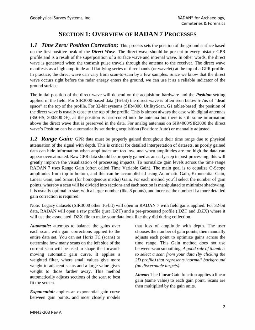
SECTION 1: OVERVIEW OF RADAN 7 PROCESSES 1.1 Time Zero/ Position Correction: This process sets the position of the ground surface based on the first positive peak of the Direct Wave. The direct wave should be present in every bistatic GPR profile and is a result of the superposition of a surface wave and internal wave. In other words, the direct wave is generated when the transmit pulse travels through the antenna to the receiver. The direct wave manifests as a high amplitude and flat-lying series of three bands (or wavelet) at the top of a GPR profile. In practice, the direct wave can vary from scan-to-scan by a few samples. Since we know that the direct wave occurs right before the radar energy enters the ground, we can use it as a reliable indicator of the ground surface.
The initial position of the direct wave will depend on the acquisition hardware and the Position setting applied in the field. For SIR3000-based data (16-bit) the direct wave is often seen below 5-7ns of “dead space” at the top of the profile. For 32-bit systems (SIR4000, UtilityScan, G1 tablet-based) the position of the direct wave is usually close to the top of the profile. This is almost always the case with digital antennas (350HS, 300/800DF), as the position is hard-coded into the antenna but there is still some information above the direct wave that is preserved in the data. For analog antennas on SIR4000/SIR3000 the direct wave’s Position can be automatically set during acquisition (Position: Auto) or manually adjusted.
1.2 Range Gain: GPR data must be properly gained throughout their time range due to physical attenuation of the signal with depth. This is critical for detailed interpretation of datasets, as poorly gained data can hide information when amplitudes are too low, and when amplitudes are too high the data can appear oversaturated. Raw GPR data should be properly gained as an early step in post-processing; this will greatly improve the visualization of processing impacts. To normalize gain levels across the time range RADAN 7 uses Range Gain (often called Time Variable Gain). The main goal is to equalize O-Scope amplitudes from top to bottom, and this can be accomplished using Automatic Gain, Exponential Gain, Linear Gain, and Smart (for homogenous media) Gain. For each method you’ll select the number of gain points, whereby a scan will be divided into sections and each section is manipulated to minimize shadowing. It is usually optimal to start with a larger number (like 8 points), and increase the number if a more detailed gain correction is required. Note: Legacy datasets (SIR3000 other 16-bit) will open in RADAN 7 with field gains applied. For 32-bit data, RADAN will open a raw profile (just .DZT) and a pre-processed profile (.DZT and .DZX) where it will use the associated .DZX file to make your data look like they did during collection.
Automatic: attempts to balance the gains over each scan, with gain corrections applied to the entire data set. You can set Horiz TC (scans) to determine how many scans on the left side of the current scan will be used to shape the forward-moving automatic gain curve. It applies a weighted filter, where small values give more weight to adjacent scans and a large value gives weight to those farther away. This method automatically adjusts sections of the scan to best fit the screen.
Exponential: applies an exponential gain curve between gain points, and most closely models
that loss of amplitude with depth. The user chooses the number of gain points, then manually adjusts each point to optimize gains across the time range. This Gain method does not use between-scan smoothing. A good rule of thumb is to select a scan from your data (by clicking the 2D profile) that represents ‘normal’ background (no discernable targets).
Linear: The Linear Gain function applies a linear gain (same value) to each gain point. Scans are then multiplied by the gain units.

Geophysical Survey Systems, Inc. RADAN® for Archaeology, Cemeteries & Forensics
3 MN43-203 Rev A
Smart: This gain method was designed for homogenous media where dielectric and conductivity are constant across the time range.
Smart gain is optimized for self-contained concrete systems such as the StructureScan Mini and StructureScan MiniXT.
Be conscious of Clipping the O-Scope peaks. While adjusting the gain points the wiggle trace must stay within the view of the O-Scope window. If the peaks extend beyond the limits of the O-Scope window, clipping will occur and data amplitudes outside the window will not be displayed. 1.3 Background Removal (Full Pass): Background Removal attempts to remove horizontal bands from datasets. These bands are usually derived from external noise, though subsurface layers are also a source. You have two options for Background removal: the Background Removal button, and the FIR-based version (see Section 1.4). The Background Removal button is the “safer” version since it applies a full pass background removal. This means it will remove horizontal reflections that extend the entire length of a given profile. In general, this will be less destructive, since real data rarely extend for such long distances while noise bands will usually extend the entire length of a profile. In complex subsurface environments, especially those that are “cluttered” with numerous targets or exhibit localized banding from near-surface features or areas of wet clay, noise bands may be interrupted and not extend the length of the profile. In these and other cases a full pass BR may not remove the bands, thus a more aggressive background removal (FIR-based, see Section 1.4) may be required.
1.4 FIR and IIR Filters: The Finite Impulse Response (FIR) and Infinite Impulse Response (IIR) processes are a combination of horizontal (scan-based) and vertical (sample-based) filters. FIR filters employ a bounding box to limit the effect of distant scans. IIR does not use a bounding box, and thus the filter length can be infinite. For archaeological datasets I rarely employ horizontal filters (except for BR – see below) and this guide will mostly deal with vertical FIR and IIR filters. The difference between FIR and IIR is the ‘aggressiveness” of the filters. FIR is not very literal, and while in the vertical dimension it will try to remove the specified frequencies it still leaves some behind. IIR is much more literal (and aggressive) and is more effective at removing unwanted frequencies.
A typical bandpass filter would use a “quarter and double” rule. For instance, a 400MHz antenna usually records a usable frequency range of 100MHz to 800MHz. In this case you could safely filter the data with a high pass of 100 and a low pass of 800. However, there is often high frequency noise pollution in data, so you could drop the low pass to 700-650 if needed. Just be careful because filtering removes real data too, not just noise. A more informed decision could be made with RADAN’s Spectrum view. To access Spectrum, right-click on a 2D profile, select Transfer, then Spectrum. You’ll notice that the vertical scale has changed to MHz, and wherever you point your mouse you will see a MHz value in your lower status bar (bottom of the RADAN window). Mouse around and figure out where the frequency spectrum is densest and then evaluate where spurious high/low frequencies extend beyond the dominant range. You can also use the Scope (Home Tab) to see a Fourier Transform of the scan.
For FIR and IIR, the vertical High Pass is the lower number – I like to think of it as “I want to keep frequencies higher than XXX”
For FIR and IIR, the vertical Low Pass is the higher number – I like to think of it as “I want to keep frequencies lower than XXX”
Geophysical Survey Systems, Inc. RADAN® for Archaeology, Cemeteries & Forensics
4 MN43-203 Rev A
FIR can be used for a customized Background Removal, and a more cautious high pass and low pass frequency filter. For FIR Background Removal, you are telling RADAN that anything horizontal/flat-lying that extends for XX number of scans is background noise and RADAN should remove it. To use it, open the FIR process and look for Horizontal and BKGR Removal. Here RADAN is asking for the number of scans, not distance. For convenience you can convert this to distance by using your scan density (typically 50 scans/meter or 18 scans/ft). With 50 scans/meter you would be collecting a new scan every 2cm. So, if you enter 100 scans in BKGR Removal, you are telling RADAN to remove all horizontal reflections that are 200cm or longer. Here you will note that this can be very dangerous with a low scan number. Always start with ~200+ scans (and use the Apply button!) to make sure you aren’t removing spatially-restricted soil layers or flat-lying archaeological features.
IIR should only be used for an aggressive vertical high pass and low pass frequency filter – I wouldn’t recommend IIR for a Background Removal. In the IIR vertical (MHz) filter, you can select the Number of Poles. The higher the number, the more aggressive/literal the high/low frequency cutoff. In comparison, a vertical FIR filter does not have poles and thus the user-specified high/low frequency cutoff is “feathered out” at the edges – this leads to a softer cut. I typically use 4 to 8 poles for vertical IIR.
You can evaluate the impact of FIR and IIR using the Spectrum view (right-click on data – transfer – spectrum). With spectrum view open, access the IIR or FIR process and enter a high and low pass (vertical) value. Press apply and observe how the frequency spectrum changes. FIR will make an obvious, but not significant, impact (unless your high/low pass values are close together or outside the central frequency). IIR, with a large number of poles, will make an increasingly aggressive impact to the frequency spectrum. Another option is to use FIR and IIR to frequency filter outside of an antenna’s central frequency. FIR will make an impact, but most of the data will remain visible; IIR (with more poles) will significantly reduce the impact of frequencies outside the specified range.
You can use IIR creatively to filter above or below an antenna’s central frequency to look at only the high frequency (higher resolution) or low frequency (lower resolution) components. You might find that some datasets are best viewed this way, since either side of the spectrum will reveal different characteristics of your dataset or perhaps a dataset is plagued by low or high frequency noise components. This can also improve 3D time slices, since you might want low frequency data for larger targets (less clutter) and high frequency data for small targets (higher resolution).
Both filters can be used in ‘real-time’ with the apply button, so use this to your advantage. Make sure you can identify what the filter is doing before you commit to it. Also, RADAN will only apply the filter to data currently on the screen so in real-time it will not apply the filter to an entire profile if it extends beyond the edge of the screen.
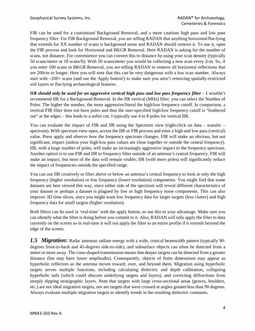
1.5 Migration: Radar antennas radiate energy with a wide, conical beamwidth pattern (typically 90-degrees front-to-back and 45-degrees side-to-side), and subsurface objects can often be detected from a meter or more away. The cone-shaped transmission means that deeper targets can be detected from a greater distance (but may have lower amplitudes). Consequently, objects of finite dimensions may appear as hyperbolic reflectors as the antenna moves toward, over, and beyond them. Migration using hyperbolic targets serves multiple functions, including calculating dielectric and depth calibration, collapsing hyperbolic tails (which could obscure underlying targets and layers), and correcting diffractions from steeply dipping stratigraphic layers. Note that targets with large cross-sectional areas (graves, boulders, etc.) are not ideal migration targets, nor are targets that were crossed at angles greater/less than 90 degrees. Always evaluate multiple migration targets to identify trends in the resulting dielectric constants.

Geophysical Survey Systems, Inc. RADAN® for Archaeology, Cemeteries & Forensics
5 MN43-203 Rev A
RADAN 7 offers two Migration methods: Hyperbolic and Kirchhoff. Hyperbolic Summation sums along a Ghost Hyperbola placed over the data and places the resulting average at the apex of the hyperbola. This process is repeated with the apex on every point in the data.
The Kirchhoff (default) method is more accurate than the Hyperbolic version. An average value is still derived by summing along a hyperbola, but Kirchhoff also applies a correction factor to the averaged value based upon the angle of incidence and distance to the target. It also applies a filter to compensate for the summation process. This filter improves resolution by emphasizing the higher frequencies and applying a phase correction. This process may require a FIR or IIR filter after completion.
Important Migration terms and their definitions:
Velocity: The speed at which the radar pulses travel through a material. The relative velocity is the ratio between the length of a hyperbolic reflector in the distance axis (in number of scans/unit) to its length in the time axis on the screen (number of samples/unit).
Dielectric: The relative dielectric permittivity is a dimensionless measure of the capacity of a material to store and transmit a charge when an electric field is applied. Dielectric varies between materials.
Time (nS): This adjusts as the peak of the Ghost Hyperbola is positioned and represents the two-way travel time to the top of the reflector.
Width: Measured in number of scans and used to sum across the data file. This value should be set to about the same number of scans as the width of hyperbolic tails in the data. Larger values tend to give more accurate results, but if the value is too large, deterioration will occur.
Gain: Increases data amplitudes after migration, usually set to a value between 1.5 and 5.
Bistatic Offset: The distance between the transmitting and receiving antennas (fixed for bistatic antennas).
1.6 Distance Normalization: Used mostly for Time-based data that were acquired without a distance encoder. For distance-based data this function is rarely used, and only then for serious distance issues (such as an improper encoder calibration).
1.7 Horizontal Scaling: Data may be modified by adjusting the Horizontal Scale using the Stacking, Skipping, and Stretching functions. Stacking (horizontal) can remove small, discreet targets (for enhancing continuous layers) or average-out vertical striping in the data caused by poor antenna coupling. Skipping will compress the data, which may be useful for profiles with long horizontal reflectors. Stretching will expand the data and may improve visualization of closely-spaced targets and horizontal reflectors. Horizontal scaling can be useful for processing 2D data, but there is no real impact on 3D time slices unless extremely high skipping or stacking values are used. A more effective Stacking filter is in the FIR and IIR processes.
1.8 Deconvolution: Deconvolution attempts to uncouple system noise and pulse width to remove multiples or “ringing” in datasets. These issues occur when the radar signal reflects back and forth between an object or layer (such as a piece of metal or layer of wet clay) and the antenna. This causes repetitive and equally-spaced reflection patterns, obscuring details at lower depths.

Geophysical Survey Systems, Inc. RADAN® for Archaeology, Cemeteries & Forensics
6 MN43-203 Rev A
RADAN 7 uses Predictive Deconvolution to approximate the shape of the transmitted pulse as the antenna is coupled to the ground. Assuming a source wavelet of a specified length (Operator Length), Deconvolution will predict what the data will look like a certain distance away (Prediction Lag), when the source wavelet is subtracted (or deconvolved) from it. This results in the compression of the reflected wavelet.
Predictable phenomena, such as antenna ringing and multiples, are moved to distances greater than the prediction lag and are effectively removed from the data.
1.9 Math Functions: For archaeological datasets there are two useful Math functions: Differentiate and Integrate. Each applies a vertical (scan-based) moving filter to enhance or downplay signal amplitudes. These are short moving filters that can achieve a vertical smoothing effect.
Differentiate evaluates the amplitude difference between two successive samples/scans (sample one, later; sample two, earlier), then subtracts the difference from sample one. The filter then considers the difference between sample two and sample three, and then subtracts the difference from scan number two. This process continues vertically until the final sample, then moves to each adjacent scan in a profile. The Differentiate filter downplays the effect of similar amplitude changes in successive samples and promotes larger amplitude changes. This means that the filter will greatly reduce the impact of small vertical amplitude changes (no real difference between samples) making larger amplitude changes more obvious in comparison. This can be useful when you want to make targets ‘pop out’ from the background. It can be useful for 2D profiles but is best used for 3D display where targets may otherwise be lost in the background.
Differentiate: y(t) = x(t) - x(t-1) Integrate evaluates the amplitude difference between two successive samples/scans (sample one, above; then sample two, below), remembers the value sample two, and then adds the difference to sample one. The filter then considers the difference between sample two and sample three, remembers the value of sample three, and then adds the difference to scan number two. This process continues vertically until the final sample, then moves to each adjacent scan in a profile. The Integrate filter can accentuate lower amplitude changes and with a lesser effect on higher amplitude changes. This means that the filter will enhance weaker signals without overaccentuating the already higher amplitudes in the data. In some ways the results of an Integrate filter look like a range gain, though Integrate could be considered
a vertical gain smoothing algorithm with a smoothing component. This can be useful when you want to prevent weaker amplitudes from being overshadowed/masked by higher amplitudes. It can be useful for 2D profiles but is best used for 3D display where high amplitudes may cause weaker amplitudes to be under-gained and difficult to see.
Integrate: y(t) = x(t) + x(t+1)
Sample Amp. Value
Retain Value Formula
Resulting Amplitude
a 10 10 b 20 b (20) b-a 10 c 22 c (22) c-b 2 d 26 d (26) d-c 4 e 50 e (50) e-d 24 f 55 f (55) f-e 5 g 34 g (34) g-f -21 h 76 h (76) h-g 42 i 78 I (78) i-h 2 j 67 j (67) j-i -11
… … … … …
Geophysical Survey Systems, Inc. RADAN® for Archaeology, Cemeteries & Forensics
7 MN43-203 Rev A
SECTION 2: PROCESSING 2D DATASETS RADAN excels at optimizing GPR data, but there are a few things you can do to optimize the software and enhance its performance. RADAN works best with a dedicated NVIDIA GPU/video card, though it can operate with an on-board Intel GPU. We recommend a higher-end CPU, like an Intel I5 or I7, and 8GB to 16GB of RAM. The software is easiest to use with a mouse; a laptop touchpad can complicate the interface.
Always set your working directory by using the Home Tab -- Global Settings. You can only set a working directory when there are no open files. This will save a lot of time and will ensure that processed data are saved in the appropriate directory.
There are two methods for saving processed data: Auto Save Yes, and Auto Save No. You’ll find these options at the top of the Global Settings window. With Auto Save on, RADAN will automatically save a new version of a dataset when a process is completed. The new file will be saved in a Proc folder in your working directory and will have a P_xxx (P_1, P_11, P_111, etc.) added to the file name. With Auto Save off, RADAN will ask you to name the output file and specify an output location. You can take advantage of this function by using a descriptive naming convention. For example, you run a Time Zero correction on File_001. When prompted to save the file, name it File_001_TZ. You then run a Background Removal on File_001_TZ, and save it as File_001_TZ_BR. Other modifiers could be Migration (_M), Range Gain (_RG), and IIR filter (_IIR_HPxxLPxx). This cumulative naming scheme will help you locate specific process iterations.
You can apply filters/processes multiple times (like Range Gain, FIR/IIR, and Math). Most filters need only be applied once. However, there are occasions where filters could be applied early in the processing steps and then again toward the end (especially Range Gain). This is because filters will often reduce overall amplitudes, as well as generate high/low frequency noise.
2.1 TIME ZERO/ POSITION CORRECTION This is typically the first process as it is important to accurately define the ground surface. Open the Time Zero process and you’ll see a red O-Scope on the left side of the screen. By default, the Method used is Manual, where the user manually positions the O-Scope. In Manual mode, left click on the O-Scope and hold down the left mouse button. You can then move the O-Scope vertically. Slide the O-Scope up or down until the center of the first positive peak (first peak of the Direct Wave) is split by the zero line. Press apply to see the result, and if it looks correct press OK. Your data will then be corrected to the ground surface. You can also use the Auto Peak method, where RADAN will automatically set the position correction.
NOTE: Time Zero uses the direct wave for positioning, so it can be difficult to set the ground surface once a Background Removal has been applied (BR removes the Direct Wave) or an aggressive IIR filter.
Geophysical Survey Systems, Inc. RADAN® for Archaeology, Cemeteries & Forensics
8 MN43-203 Rev A
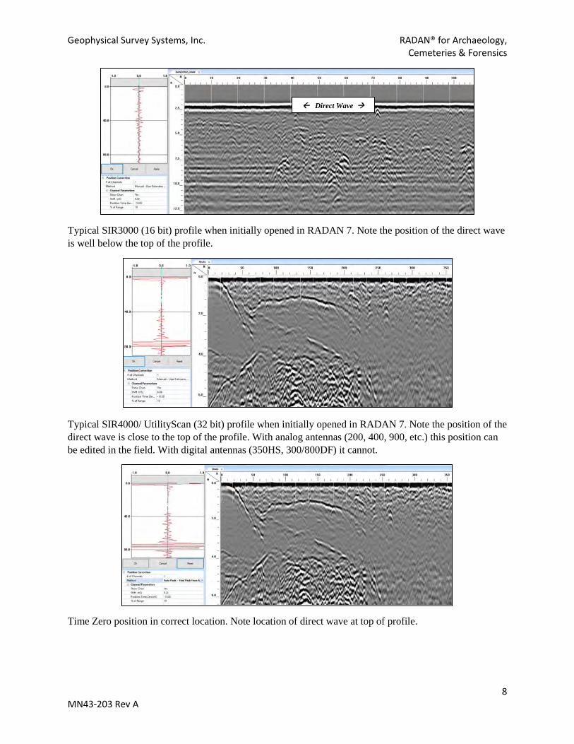
Typical SIR3000 (16 bit) profile when initially opened in RADAN 7. Note the position of the direct wave is well below the top of the profile.
Typical SIR4000/ UtilityScan (32 bit) profile when initially opened in RADAN 7. Note the position of the direct wave is close to the top of the profile. With analog antennas (200, 400, 900, etc.) this position can be edited in the field. With digital antennas (350HS, 300/800DF) it cannot.
Time Zero position in correct location. Note location of direct wave at top of profile.
Direct Wave
Geophysical Survey Systems, Inc. RADAN® for Archaeology, Cemeteries & Forensics
9 MN43-203 Rev A
2.2 BACKGROUND REMOVAL The purpose of Background Removal [BR] is to identify and eliminate flat-lying horizontal reflections. These bands are usually derived from external low frequency noise, ringing/multiples from boundaries with high reflection coefficients, or other variables in less-than-ideal soil conditions. There are multiple BR methods, including Full Pass and manual/scan-based. For Full Pass, RADAN looks for horizontal bands that extend the entire length of a given profile. This is the safest method since it is not as likely to remove real data. Manual/scan-based methods offer more versatility and customization, but with a low number of scans the BR can remove a significant amount of real data. Profiles with short but consistent noise bands can make good use of a creative BR, whereby a relatively small number of scans (50-100) may remove stubborn noise while preserving most of the real data. As with any post-processing step, BR should be used only when needed, and is best used with full knowledge of what the process actually does.
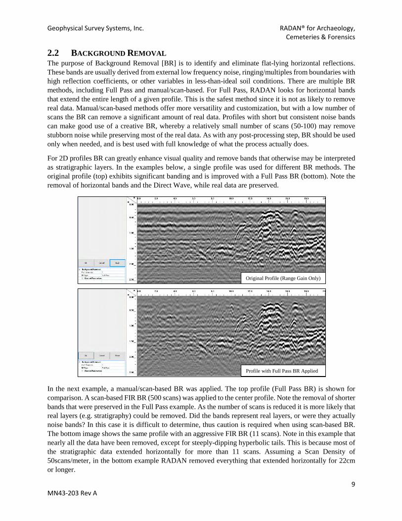
For 2D profiles BR can greatly enhance visual quality and remove bands that otherwise may be interpreted as stratigraphic layers. In the examples below, a single profile was used for different BR methods. The original profile (top) exhibits significant banding and is improved with a Full Pass BR (bottom). Note the removal of horizontal bands and the Direct Wave, while real data are preserved.
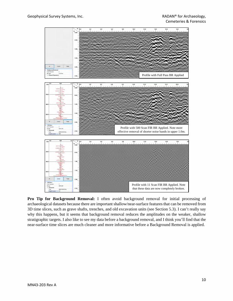
In the next example, a manual/scan-based BR was applied. The top profile (Full Pass BR) is shown for comparison. A scan-based FIR BR (500 scans) was applied to the center profile. Note the removal of shorter bands that were preserved in the Full Pass example. As the number of scans is reduced it is more likely that real layers (e.g. stratigraphy) could be removed. Did the bands represent real layers, or were they actually noise bands? In this case it is difficult to determine, thus caution is required when using scan-based BR. The bottom image shows the same profile with an aggressive FIR BR (11 scans). Note in this example that nearly all the data have been removed, except for steeply-dipping hyperbolic tails. This is because most of the stratigraphic data extended horizontally for more than 11 scans. Assuming a Scan Density of 50scans/meter, in the bottom example RADAN removed everything that extended horizontally for 22cm or longer.
Original Profile (Range Gain Only)
Profile with Full Pass BR Applied
Geophysical Survey Systems, Inc. RADAN® for Archaeology, Cemeteries & Forensics
10 MN43-203 Rev A
Pro Tip for Background Removal: I often avoid background removal for initial processing of archaeological datasets because there are important shallow/near-surface features that can be removed from 3D time slices, such as grave shafts, trenches, and old excavation units (see Section 5.3). I can’t really say why this happens, but it seems that background removal reduces the amplitudes on the weaker, shallow stratigraphic targets. I also like to see my data before a background removal, and I think you’ll find that the near-surface time slices are much cleaner and more informative before a Background Removal is applied.
Profile with 500 Scan FIR BR Applied. Note more effective removal of shorter noise bands in upper 1.0m.
Profile with 11 Scan FIR BR Applied. Note that these data are now completely broken.
Profile with Full Pass BR Applied
Geophysical Survey Systems, Inc. RADAN® for Archaeology, Cemeteries & Forensics
11 MN43-203 Rev A
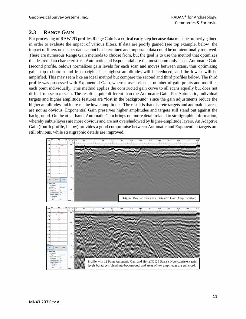
2.3 RANGE GAIN For processing of RAW 2D profiles Range Gain is a critical early step because data must be properly gained in order to evaluate the impact of various filters. If data are poorly gained (see top example, below) the impact of filters on deeper data cannot be determined and important data could be unintentionally removed. There are numerous Range Gain methods to choose from, but the goal is to use the method that optimizes the desired data characteristics. Automatic and Exponential are the most commonly used. Automatic Gain (second profile, below) normalizes gain levels for each scan and moves between scans, thus optimizing gains top-to-bottom and left-to-right. The highest amplitudes will be reduced, and the lowest will be amplified. This may seem like an ideal method but compare the second and third profiles below. The third profile was processed with Exponential Gain, where a user selects a number of gain points and modifies each point individually. This method applies the constructed gain curve to all scans equally but does not differ from scan to scan. The result is quite different than the Automatic Gain. For Automatic, individual targets and higher amplitude features are “lost in the background” since the gain adjustments reduce the higher amplitudes and increase the lower amplitudes. The result is that discrete targets and anomalous areas are not as obvious. Exponential Gain preserves higher amplitudes and targets still stand out against the background. On the other hand, Automatic Gain brings out more detail related to stratigraphic information, whereby subtle layers are more obvious and are not overshadowed by higher-amplitude layers. An Adaptive Gain (fourth profile, below) provides a good compromise between Automatic and Exponential: targets are still obvious, while stratigraphic details are improved.
Original Profile: Raw GPR Data (No Gain Amplification)
Profile with 11 Point Automatic Gain and HorizTC (25 Scans). Note consistent gain levels but targets blend into background, and areas of low amplitudes are enhanced.

Geophysical Survey Systems, Inc. RADAN® for Archaeology, Cemeteries & Forensics
12 MN43-203 Rev A
Keep in mind these Range Gain methods and their relative strengths and weaknesses. We’ll see later that some of the methods are much more appropriate for 3D data, and some reduce 3D interpretability.
SPOILER ALERT: You will likely find that an Exponential Range Gain is the best method for optimizing 3D datasets. [Optimizing both vertical and horizontal gain levels is not always advantageous]
2.4 FIR AND IIR (MAY REQUIRE SECOND RANGE GAIN AFTER FILTERING)
Low- to mid-frequency GPR data (200-900MHz) often exhibit spurious frequency-derived noise from external EM sources. Common sources of interference in the US include the FM Radio band (87.5-108MHz), VHF band (174-216MHz), UHF band (470-806MHz) 700MHz Service (698-806MHz), and the 800MHz Cellular Service (824-849MHz; 869-894MHz). Most of these frequency bands overlap with the frequency spectrum of 200-900MHz antennas, with stronger interference with increasing proximity to the source. For example, a 400MHz antenna transmits and receives a usable spectrum from 100MHz to 800Mhz. Typical IIR filters during 400MHz data acquisition are Low Pass 800MHz and High Pass 100MHz. With these filters applied, there is still interference from VHF, UHF, and the 700MHz Service. Cell phone interference can occur when a device is close to the antenna. Using IIR and FIR filters these frequencies can be removed or their impact can be diminished.
Exponential Range Gain, 10 points. Note difference between Exponential and Automatic (above), especially the “masking” effect of auto gains for discrete targets (in this case human graves). Auto Gain can amplify weaker amplitudes, which can often be diagnostic signatures.
Adaptive Gain (Fast) with 4 Points. Similar to Automatic Gain but Overall Amplitudes are Enhanced. Targets (Graves) can blend into Background.
Geophysical Survey Systems, Inc. RADAN® for Archaeology, Cemeteries & Forensics
13 MN43-203 Rev A
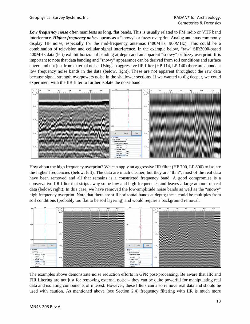
Low frequency noise often manifests as long, flat bands. This is usually related to FM radio or VHF band interference. Higher frequency noise appears as a “snowy” or fuzzy overprint. Analog antennas commonly display HF noise, especially for the mid-frequency antennas (400MHz, 900MHz). This could be a combination of television and cellular signal interference. In the example below, “raw” SIR3000-based 400MHz data (left) exhibit horizontal banding at depth and an apparent “snowy” or fuzzy overprint. It is important to note that data banding and “snowy” appearance can be derived from soil conditions and surface cover, and not just from external noise. Using an aggressive IIR filter (HP 114, LP 140) there are abundant low frequency noise bands in the data (below, right). These are not apparent throughout the raw data because signal strength overpowers noise in the shallower sections. If we wanted to dig deeper, we could experiment with the IIR filter to further isolate the noise band.
How about the high frequency overprint? We can apply an aggressive IIR filter (HP 700, LP 800) to isolate the higher frequencies (below, left). The data are much cleaner, but they are “thin”; most of the real data have been removed and all that remains is a constricted frequency band. A good compromise is a conservative IIR filter that strips away some low and high frequencies and leaves a large amount of real data (below, right). In this case, we have removed the low-amplitude noise bands as well as the “snowy” high frequency overprint. Note that there are still horizontal bands at depth; these could be multiples from soil conditions (probably too flat to be soil layering) and would require a background removal.
The examples above demonstrate noise reduction efforts in GPR post-processing. Be aware that IIR and FIR filtering are not just for removing external noise – they can be quite powerful for manipulating real data and isolating components of interest. However, these filters can also remove real data and should be used with caution. As mentioned above (see Section 2.4) frequency filtering with IIR is much more
Geophysical Survey Systems, Inc. RADAN® for Archaeology, Cemeteries & Forensics
14 MN43-203 Rev A
aggressive and literal than frequency filtering with a FIR filter. In the examples below, a single profile was filtered using various parameters with IIR and FIR filters. Note the use of Spectrum view to evaluate the effect of the filters on the frequency spectrum. This is a more scientific method for choosing the proper frequency filter parameters, rather than guessing or pressing apply/reset.
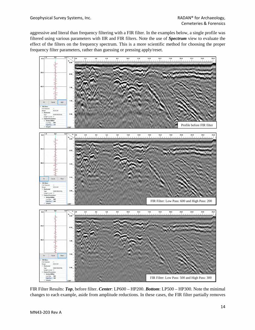
FIR Filter Results: Top, before filter. Center: LP600 – HP200. Bottom: LP500 – HP300. Note the minimal changes to each example, aside from amplitude reductions. In these cases, the FIR filter partially removes
Profile before FIR filter
FIR Filter: Low Pass: 600 and High Pass: 200
FIR Filter: Low Pass: 500 and High Pass: 300

Geophysical Survey Systems, Inc. RADAN® for Archaeology, Cemeteries & Forensics
15 MN43-203 Rev A
the unwanted frequencies, but is not aggressive enough to remove all of them. See images below for related Spectrum view.
FIR Filter (Spectrum): Top, before filter. Center: LP600 – HP200. Bottom: LP500 – HP300. Note the minimal changes to each frequency spectrum. In these cases, the FIR filter partially removes the unwanted frequencies, but is not aggressive enough to remove all of them. This is especially obvious in the unnoticeable changes with an aggressive HP/LP cut (300-500MHz).
Spectrum View: FIR Filter: Low Pass: 600 and High Pass: 200
Spectrum View: FIR Filter: Low Pass: 500 and High Pass: 300
Spectrum View: before FIR Filter

Geophysical Survey Systems, Inc. RADAN® for Archaeology, Cemeteries & Forensics
16 MN43-203 Rev A
IIR Filter Results (1 Pole): Top, before filter. Center: LP600 – HP200. Bottom: LP500 – HP300. A 1-pole IIR produces similar results to a FIR filter.
Profile before IIR filter
IIR Filter: Low Pass: 600 and High Pass: 200
IIR Filter: Low Pass: 500 and High Pass: 300
Geophysical Survey Systems, Inc. RADAN® for Archaeology, Cemeteries & Forensics
17 MN43-203 Rev A
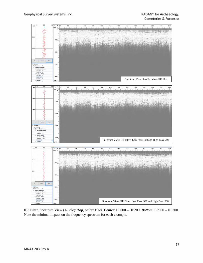
IIR Filter, Spectrum View (1-Pole): Top, before filter. Center: LP600 – HP200. Bottom: LP500 – HP300. Note the minimal impact on the frequency spectrum for each example.
Spectrum View: Profile before IIR filter
Spectrum View: IIR Filter: Low Pass: 600 and High Pass: 200
Spectrum View: IIR Filter: Low Pass: 500 and High Pass: 300
Geophysical Survey Systems, Inc. RADAN® for Archaeology, Cemeteries & Forensics
18 MN43-203 Rev A
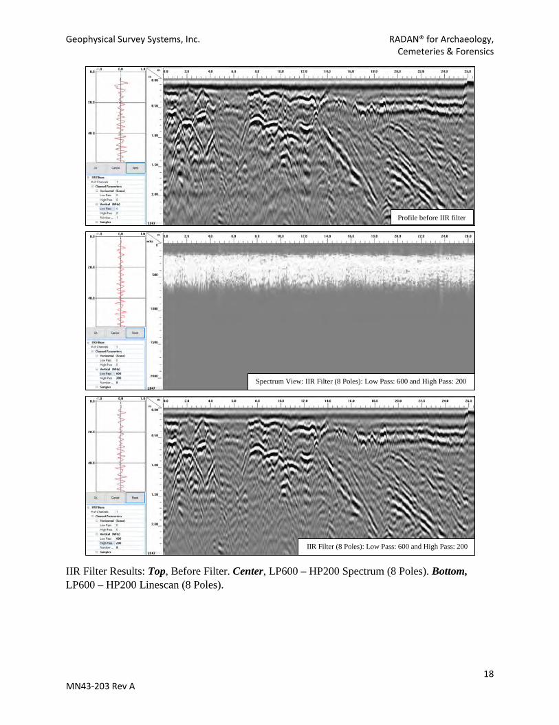
IIR Filter Results: Top, Before Filter. Center, LP600 – HP200 Spectrum (8 Poles). Bottom, LP600 – HP200 Linescan (8 Poles).
Profile before IIR filter
Spectrum View: IIR Filter (8 Poles): Low Pass: 600 and High Pass: 200
IIR Filter (8 Poles): Low Pass: 600 and High Pass: 200

Geophysical Survey Systems, Inc. RADAN® for Archaeology, Cemeteries & Forensics
19 MN43-203 Rev A
IIR Filter Results: Top, Before Filter. Center, LP500 – HP300 Spectrum (8 Poles). Bottom, LP500 – HP300 Linescan (8 Poles). This is an aggressive bandpass that will remove most frequencies outside the specified range.
Profile before IIR filter
Spectrum View: IIR Filter (8 Poles): Low Pass: 500 and High Pass: 300
IIR Filter (8 Poles): Low Pass: 500 and High Pass: 300

Geophysical Survey Systems, Inc. RADAN® for Archaeology, Cemeteries & Forensics
20 MN43-203 Rev A
IIR Filter Results: Top, Before Filter. Center, LP300 – HP87 Spectrum (8 Poles) showing low frequency components. Bottom, LP800 – HP350 Linescan (8 Poles) showing high frequency components. This is a powerful method for viewing only high or low frequency data components.
Profile before IIR filter
IIR Filter (8 Poles): Low Pass: 300 and High Pass: 87
IIR Filter (8 Poles): Low Pass: 800 and High Pass: 350

Geophysical Survey Systems, Inc. RADAN® for Archaeology, Cemeteries & Forensics
21 MN43-203 Rev A
2.5 MIGRATION (CONSIDER CHANGING YOUR COLOR TABLE TO #18 OR #22) When the Migration process is activated, the left pane will display the Migration Process Bar and a Ghost Hyperbola will appear on the left side of the Linescan. Click anywhere on the 2D profile and the Ghost Hyperbola will move to that location. The Ghost Hyperbola is a tool to help identify the correct velocity/dielectric of subsurface materials.
Method: Choose either Kirchhoff (default) or Hyperbolic.
Hyperbola Fitting: adjust the shape of the Ghost Hyperbola to fit over a hyperbola in your data. Notice that as the shape of the hyperbola changes, so does the velocity/dielectric. The shape of the Ghost Hyperbola can be adjusted using the Process Pane (by moving the black square) or on the Linescan data (by using the available drag handles). Once the shape is set, make sure to adjust the width bars to set the width of the hyperbolic target in your data (vertical bars around Ghost Hyperbola).
In complex stratigraphic settings the dielectric could vary considerably from shallower to deeper layers. In these cases, you can use a Variable Velocity Migration if multiple hyperbolas are available at different depths. With this method two or more Ghost Hyperbolas are used at different depths to provide a better overall average of dielectric across the vertical range.
Note that Variable Velocity Migration is useful for ‘cleaning up’ 3D data and evaluating dielectric changes with depth. However, compared with a single hyperbolic migration it is not as accurate for time-to-depth calibration
Select the shallowest hyperbola first and do a regular hyperbola fitting.
Double-click in the Velocity Plot to add a second box. This will create a new Ghost Hyperbola to fit over another hyperbolic target. Perform a hyperbola fitting on the second hyperbola.
Continue to double-click, creating additional boxes and performing hyperbola fitting.
Click Apply to test the Migration and, if necessary, click Reset and re-adjust. The Ghost Hyperbola was a good fit if the dipping sides of the reflector are removed as seen in the image below.
Once satisfied with the Migration, click OK.
Pro Tip: 2D data are best interpreted with hyperbolic tails, and 3D data are much improved when hyperbolic tails are removed. To ‘migrate’ 2D data without losing hyperbolic tails, open the Migration process, fit the hyperbolic target, then write down the resulting dielectric. Press Cancel. Open the File header for your current data, then type in the dielectric. This will correct the depth scale while preserving hyperbolic tails.
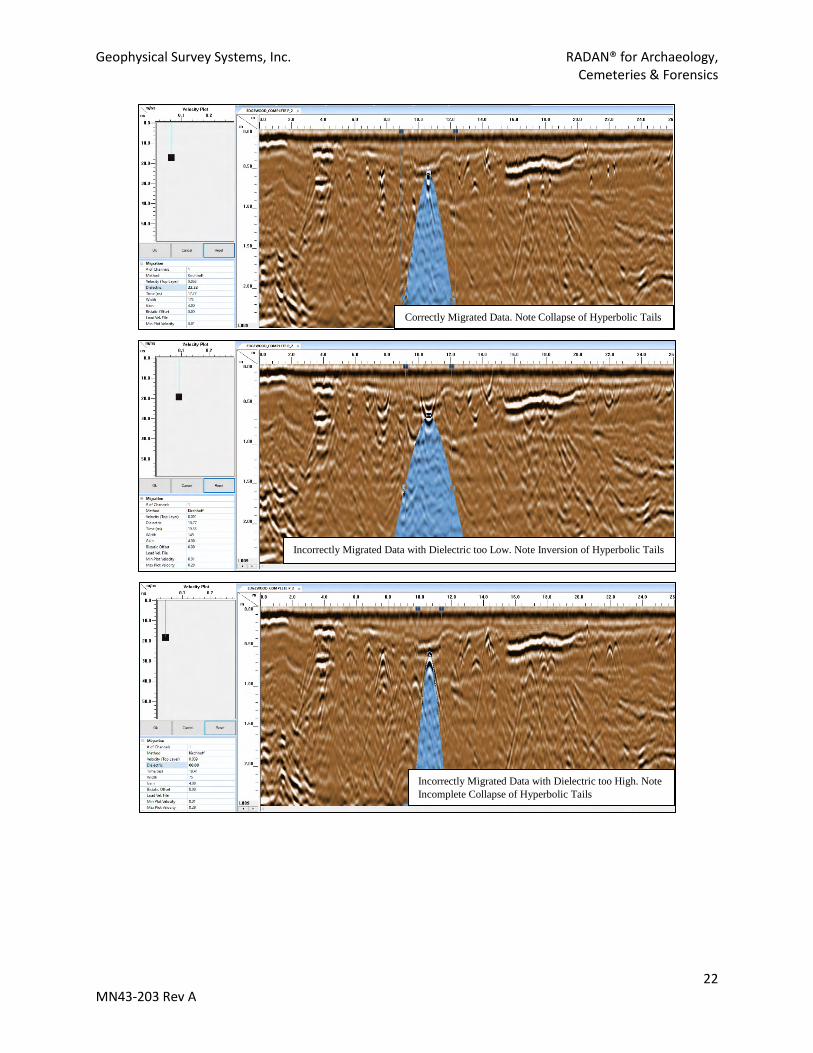
Data before Migration, showing Ghost Hyperbola (Dirt Color Table)
Geophysical Survey Systems, Inc. RADAN® for Archaeology, Cemeteries & Forensics
22 MN43-203 Rev A
Correctly Migrated Data. Note Collapse of Hyperbolic Tails
Incorrectly Migrated Data with Dielectric too Low. Note Inversion of Hyperbolic Tails
Incorrectly Migrated Data with Dielectric too High. Note Incomplete Collapse of Hyperbolic Tails

Geophysical Survey Systems, Inc. RADAN® for Archaeology, Cemeteries & Forensics
23 MN43-203 Rev A
2.6 Mathematical Functions
Differentiate and Integrate (may require additional Range Gain)
Original Profile
Differentiate Function. Note Downplay of Low Amplitudes Relative to Higher Amplitudes.
Integrate Function. Note Accentuation of Low Amplitudes without Over-Gaining Higher Amplitudes
Geophysical Survey Systems, Inc. RADAN® for Archaeology, Cemeteries & Forensics
24 MN43-203 Rev A
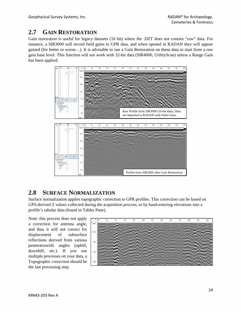
2.7 GAIN RESTORATION Gain restoration is useful for legacy datasets (16 bit) where the .DZT does not contain “raw” data. For instance, a SIR3000 will record field gains to GPR data, and when opened in RADAN they will appear gained (for better or worse…). It is advisable to run a Gain Restoration on these data to start from a raw gain base level. This function will not work with 32-bit data (SIR4000, UtilityScan) unless a Range Gain has been applied.
2.8 SURFACE NORMALIZATION Surface normalization applies topographic correction to GPR profiles. This correction can be based on GPS-derived Z values collected during the acquisition process, or by hand-entering elevations into a profile’s tabular data (found in Tables Pane).
Note: this process does not apply a correction for antenna angle, and thus it will not correct for displacement of subsurface reflections derived from various penetration/tilt angles (uphill, downhill, etc.). If you use multiple processes on your data, a Topographic correction should be the last processing step.
Raw Profile from SIR3000 (16-bit data). Data are Imported to RADAN with Field Gains.
Profile from SIR3000 after Gain Restoration.
Geophysical Survey Systems, Inc. RADAN® for Archaeology, Cemeteries & Forensics
25 MN43-203 Rev A
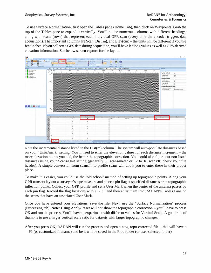
To use Surface Normalization, first open the Tables pane (Home Tab), then click on Waypoints. Grab the top of the Tables pane to expand it vertically. You’ll notice numerous columns with different headings, along with scans (rows) that represent each individual GPR scan (every time the encoder triggers data acquisition). The important columns are Scan, Dist(m), and Elev(cm) – the units will be different if you use feet/inches. If you collected GPS data during acquisition, you’ll have lat/long values as well as GPS-derived elevation information. See below screen capture for the layout:
Note the incremental distance listed in the Dist(m) column. The system will auto-populate distances based on your “Units/mark” setting. You’ll need to enter the elevation values for each distance increment – the more elevation points you add, the better the topographic correction. You could also figure out non-listed distances using your Scans/Unit setting (generally 50 scans/meter or 12 to 18 scans/ft; check your file header). A simple conversion from scans/m to profile scans will allow you to enter these in their proper place.
To make this easier, you could use the ‘old school’ method of setting up topographic points. Along your GPR transect lay out a surveyor’s tape measure and place a pin flag at specified distances or at topographic inflection points. Collect your GPR profile and set a User Mark when the center of the antenna passes by each pin flag. Record the flag locations with a GPS, and then enter them into RADAN’s Tables Pane on the scans that have an associated User Mark.
Once you have entered your elevations, save the file. Next, use the “Surface Normalization” process (Processing tab). Note: Using Apply/Reset will not show the topographic correction – you’ll have to press OK and run the process. You’ll have to experiment with different values for Vertical Scale. A good rule of thumb is to use a larger vertical scale ratio for datasets with larger topographic changes. After you press OK, RADAN will run the process and open a new, topo-corrected file – this will have a __P1 (or customized filename) and be it will be saved in the Proc folder (or user-selected folder).

Geophysical Survey Systems, Inc. RADAN® for Archaeology, Cemeteries & Forensics
26 MN43-203 Rev A
2.9 Deconvolution Select Deconvolution from the Processing Tab. Note that most GPR data will only have one channel. Right click the vertical scale and change it to samples.
Operator Length: The size of the filter, equaling the number of samples making up 1 pulse length (see Appendix II) Longer filters achieve a better approximation of the radar wavelet and generally give better results. The operator length should be about one full cycle of the radar antenna wavelet. A value less than this gives poor results. Using your mouse cursor, measure the peak-to-peak width of a multiple in number of samples. Enter this value into Operator Length. Increase the operator length slightly for more effect. Prediction Lag: the desired length of the output pulses, usually about one-half cycle of the antenna wavelet. Anything smaller than this will produce more noise. Prediction Lag should be equal to or less than the spacing between multiples. A prediction lag between 5 and 1 is used to approximate “spiking” deconvolution, which matches and removes the wavelet. However, this introduces noise into the data.
Prewhitening: Modifies the autocorrelation function by boosting the white noise (zero delay) component. Prewhitening stabilizes the filter, thereby smoothing the output and reducing noise. Values between 1 and 10 percent are common, 8 percent is a good value to start with. Overall Gain: The deconvolution process attenuates/weakens the signal, especially when the prediction lag is short. Gain values of 3 to 5 are common, but use whatever value achieves an amplitude level equal to the original data. Samples: The starting and ending sample should be set to establish the “time gate," specified in terms of sample number, in which the Deconvolution filter is active. For instance, a start sample and end sample of 256 and 512 respectively may be used to remove multiples beneath a reflector located at sample number 256 in a 512 Samples/Scan data set.
Click Apply and Reset and adjust if necessary. Click OK once the desired results are achieved or cancel to close the processing window without applying the filter.

Geophysical Survey Systems, Inc. RADAN® for Archaeology, Cemeteries & Forensics
27 MN43-203 Rev A
Before Deconvolution After Deconvolution
2.10 Hilbert Transform This process is usually reserved for 3D datasets. Of the three options (Magnitude, Phase, Frequency) only Magnitude is recommended – the others are not relevant to archaeological datasets. Reflector amplitude and time are the primary types of GPR information. Using a spatial envelope, a Hilbert Transform provides a different way of defining the data by transforming phase (positive or negative changes in the scan trace) to an absolute magnitude (stripping the positive/negative phase components). This process thereby calculates a truer representation of total reflected energy, which can be more sensitive to important subsurface dielectric changes.

Geophysical Survey Systems, Inc. RADAN® for Archaeology, Cemeteries & Forensics
28 MN43-203 Rev A
2.11 Horizontal Scaling This option can be useful for processing 2D data, as it is one of the only methods for compressing or expanding a profile’s Scan Density (Scans/Unit). For example, field data were collected at 100 scans/meter, but compressing to 50 scans/meter may improve the interpretability of the data. Horizontal Scaling has no real impact on 3D time slices unless extreme Stretching or Skipping values are used, or a large Stacking value is applied. With Stacking, successive scans are merged and this applies a smoothing factor to the data. Large Stacking values will horizontally “smear” the data, which can distort reflector geometry.

Geophysical Survey Systems, Inc. RADAN® for Archaeology, Cemeteries & Forensics
29 MN43-203 Rev A
2.12 Edit Block GPR profiles may require vertical trimming to shorten the time/depth scale, or horizontal clipping to select a certain distance range or subset of a profile. This is particularly important when more than half of a profile’s time range is attenuated and not usable (vertical) or profiles are longer than intended (horizontal). The Edit Block function can trim the vertical and horizontal scales, where sections of the data can be deleted or saved to create a new file. The original data are not modified as part of this process.
I recommend that you change the color palette (Home Tab – Color Tables) prior to performing Edit Block – this will make the overlay easier to manipulate. I also suggest changing the horizontal scale to Scans. Then, look at your Tables Pane (activate on the Home tab) and scroll to the bottom of the Waypoints tab. This will tell you how many scans are contained in the profile. Alternatively, with the horizontal scale set to Scans you can mouse over the profile and identify the scan number at a location of interest.
When the Edit Block icon is selected from the Adjust Scans Group, the left pane will display the Edit Block Process Bar. Click Block Operation and select Save (save the
selected area to a new file) or Delete (delete the selected area from the original data and save a new file without the deleted area).
Select the Area: There are two ways to choose the area that to delete or save. 1) Adjust the picking tool overlay that appears
on the linescan to highlight the part of the data to save or delete. To do this, simply grab the handles of the picking tool overlay, which will first appear on the left side of the linescan and drag the mouse to area of
interest. While maneuvering the picking tool overlay on the linescan the Start Scan, End Scan, and Start and End Samples will update accordingly.
2) Manually adjust the Start Scan, End Scan, and Start and End Samples in the Edit Block Bar.
Click OK to process or Cancel to discard the operation.
Geophysical Survey Systems, Inc. RADAN® for Archaeology, Cemeteries & Forensics
30 MN43-203 Rev A
2.13 2D INTERACTIVE (SAVE EARLY AND OFTEN!) 2D interactive provides a digitizing environment where targets or layers can be traced throughout a dataset. Points can then be exported as a text file of X and Y coordinates (or Lat(Y) and Long(X) if GPS data are available), along with amplitude, depth, two-way travel time (TWTT) velocity/dielectric, and other export options. This is quite useful for archaeological data, as a text file of digitized points can be imported into other programs, such as ESRI’s ArcGIS or Golden Software’s Surfer. The most effective method for archaeological and forensic datasets is the LAYER option, where individual points are digitized. The Target option is not as useful; it attempts to connect points across multiple profiles, thus creating polylines.
For individual targets (graves, features, etc.) consider assigning a new layer for different target/layer classes or individual stratigraphic layers. For instance, graves could be digitized in Layer 1, pit features in Layer 2, etc. You can then export all relevant layers (see below) into one text file. To keep things organized, consider multiple passes where each one focuses on a single target type or stratigraphic unit.
Note: RADAN prefers GPS coordinates in Decimal Degrees (DecDeg) as do other programs that import tabular data. Before exporting 2D Interactive picks (with GPS data) I suggest setting GPS display to DecDeg (in View tab).
When exporting points, you should use filtering (see below) to remove unwanted data. By default, RADAN will export all scans from the dataset and you’d have to filter a large dataset in Excel after export. In this case, the points picked with 2D interactive would be the only ones with values for chosen export fields (like amplitude and depth). You’d have to sort by descending order and select only those rows with data for export fields, then cut/paste into another file. It is much easier to use RADAN to filter before export, especially in large datasets with tens of thousands of picks and scans.
Interactive Status Group Show: Toggles On or Off the targets and layers already added to the data.
Add or Edit: When selected, displays the targets or layers already added. You can edit the existing interpretations or add new ones.
Objects Group Pick Type: There are two types of objects that can be added to the data; Targets or Layers. For archaeological, forensic, and cemetery data the Layer option is the best choice. Only the Layer option will be discussed in this guide.
Focus: This specifies which Layer is being added or modified. Use the dropdown menu to change between layers. This will be useful for digitizing different dataset components. For instance, Layer 1 could contain points digitized on possible graves, while layer 2 could contain points on potential archaeological features, and Layer 3 might be used to digitize the base of the plow zone (ApZ). Don’t forget to write down what each Layer represents and remember to switch to the correct layer when adding new points.
Pick Attributes GroupPick Polarity: When picking targets or layers, the user may specify which portion of the reflection to attach new picks to Positive, Negative, Absolute, or None polarity. For archaeological datasets I usually change Pick Polarity to None.
Search Width: In pixels, enter the search width for the Single Point picking tool. Only useful if specifying Pick Polarity.
Geophysical Survey Systems, Inc. RADAN® for Archaeology, Cemeteries & Forensics
31 MN43-203 Rev A
Pick Tool Group Disabled: Disable Picking Tool.
Single Point: Enter a single point when target picking. A left mouse click adds a point and a right mouse click deletes a point.
Select Block: The Select Block picking tool is designed to operate over a large number of scans. When Select Block is activated a translucent square appears over the data when the user clicks the left mouse button. The select block contains tiny squares on each face and corner for resizing.
Select Range: When Select Range is activated a translucent overlay appears over the data, extending the entire length of the profile. It operates similarly to the Select Block, except that all operations performed using the Select Range picking tool are performed within the time interval (slice width) of the selected area on all the scans in the file. The slice width is adjusted by clicking the left mouse button on one of the handles (located at the top and bottom at the horizontal midpoint of the slice) and dragging the handle to the desired location.Select Block and Select Range The following options are accessed by right-clicking within the block or range selected.
Add Points: Will activate the program to begin a smart search for reflection peaks within the selected region. Circles will overlay the data where reflection peaks are identified by the search algorithm. Picks will be added to whichever Target or Layer is currently active (i.e. in Focus).
Delete Points: Will delete the picks of the current Target or Layer located within the selected region.
Pick Modification Options Change Pick ID: Change the layer or target number assigned to the picks located within the selected region. For example, the user desires to change the layer # of a group of Layer 3 picks to Layer 2. The user must select layer 3 as the Current Layer, position the Select Block (or Select Range) over the group of points and click the right mouse button to access the Pick Modification Options. Select Change Pick ID to switch from Layer 3 to Layer 2.
Change Pick Velocity: Changes the velocity of the currently selected layer picks located in the selected region. It opens a dialog box for entering the desired velocity. The user can choose to either specify the new velocity, use the nearest core, or ground truth, data, or use results from velocity analysis. Choosing Lock Velocity keeps the data from being change with subsequent velocity modifications.
Interpolate Points: Will interpolate layer picks (add new picks between existing ones) using the interpolation method (Linear or Nearest Neighbor) specified in Global Parameters under Interpolation Method.
Ground Truth: Selecting the Ground Truth icon allows the user to individually adjust the depth of picks based upon a true measured depth. As depths are entered, they appear in the Target or Layer Ground Truth tab of the Table Pane. To enter Ground Truth info, select Ground Truth from the Interactive Tab. Click where the core/other data was collected and enter the depth. Click OK or cancel.
To specify all new layer picks to have velocities calculated from Ground Truth or Migration, change the Vel. Method from Default Vel. to Core Data in the Layer tab of the Table.
Geophysical Survey Systems, Inc. RADAN® for Archaeology, Cemeteries & Forensics
32 MN43-203 Rev A
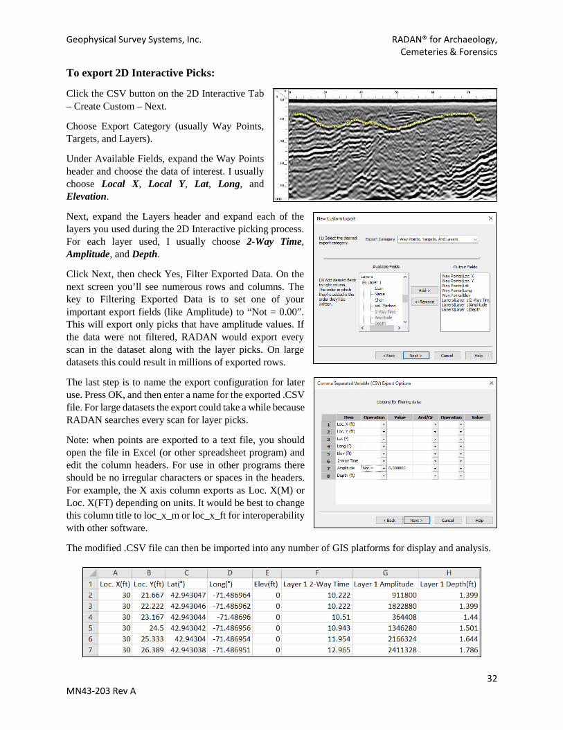
To export 2D Interactive Picks:
Click the CSV button on the 2D Interactive Tab – Create Custom – Next.
Choose Export Category (usually Way Points, Targets, and Layers).
Under Available Fields, expand the Way Points header and choose the data of interest. I usually choose Local X, Local Y, Lat, Long, and Elevation.
Next, expand the Layers header and expand each of the layers you used during the 2D Interactive picking process. For each layer used, I usually choose 2-Way Time, Amplitude, and Depth.
Click Next, then check Yes, Filter Exported Data. On the next screen you’ll see numerous rows and columns. The key to Filtering Exported Data is to set one of your important export fields (like Amplitude) to “Not = 0.00”. This will export only picks that have amplitude values. If the data were not filtered, RADAN would export every scan in the dataset along with the layer picks. On large datasets this could result in millions of exported rows.
The last step is to name the export configuration for later use. Press OK, and then enter a name for the exported .CSV file. For large datasets the export could take a while because RADAN searches every scan for layer picks.
Note: when points are exported to a text file, you should open the file in Excel (or other spreadsheet program) and edit the column headers. For use in other programs there should be no irregular characters or spaces in the headers. For example, the X axis column exports as Loc. X(M) or Loc. X(FT) depending on units. It would be best to change this column title to loc_x_m or loc_x_ft for interoperability with other software.
The modified .CSV file can then be imported into any number of GIS platforms for display and analysis.

Geophysical Survey Systems, Inc. RADAN® for Archaeology, Cemeteries & Forensics
33 MN43-203 Rev A
After exporting 2D Interactive layer picks, you can then import them into another software platform. A good example is shown below. Layer picks were digitized from a cave dataset and imported to Surfer for a 3D reconstruction of the bedrock beneath the cave sediments.
2.14 USING GPS DATA WITH 2D PROFILES The most convenient method for adding GPS data to GPR profiles is to connect a GPS during data acquisition. For SIR3000 control units a Serial Data Recorder should be used, otherwise only the start/end GPS positions will be written to the file header (refer to the SIR3000 manual for details). Other units (32-bit) connect directly to a GPS without a SDR, such as SIR4000 (9-pin serial, external), UtilityScan Tablet (9-pin serial, external), and UtilityScan (Bluetooth external/ internal). The 32-bit systems generate a .DZG file along with the standard .DZT and .DZX files. If all files are in the same directory RADAN will import the GPS data when the .DZT is opened. You can then mouse around on the profile and view latitude/longitude and elevation (look for the status bar at the bottom of the screen). Click the Location button (Home Tab) and view the GPS trackline and individual GPS points. The points can be dragged to new locations, which is useful for obvious GPS errors (near buildings, tree canopy, etc.). Click the 3D View button (Home Tab) to view your profile in 3D (fit to GPS trackline). GPS data can also be used for Surface Normalization (Section 2.8), and to export 2D Interactive picks (Section 2.13) with lat/long coordinates.

Geophysical Survey Systems, Inc. RADAN® for Archaeology, Cemeteries & Forensics
34 MN43-203 Rev A
RADAN will also allow manually-entered GPS data for a single GPR profile, including elevation data. The ideal method is to collect straight profiles and use a GPS to record the start/end locations. For complex lines, or for better precision, you could lay out a surveyor’s tape and place a pin flag at specified distances. Set a User Mark when the center of the antenna passes by each pin flag. Record the flag locations with a GPS or total station, and then enter them into RADAN’s Tables Pane for scans with an associated User Mark.
RADAN’s Google Earth functions (Google Earth Tab) can export tracklines for GPS-encoded 2D Profiles. You can also export Layer and Target picks, User Marks, and Ground Truth locations. In most cases
Profile before GPS-based Surface Normalization
Profile after GPS-based Surface Normalization
Trackline from GPS-encoded data GPR profile fit to GPS trackline

Geophysical Survey Systems, Inc. RADAN® for Archaeology, Cemeteries & Forensics
35 MN43-203 Rev A
exporting the GPS Track (as a .KML) is the most useful, since the tracks can be viewed on modern aerials. You could also use GIS software to convert the .KML to a shapefile or other format.
2.15 EXPORTING 2D DATA FROM RADAN There are numerous methods for exporting 2D data from RADAN. A single profile, or multiple profiles from a gridded dataset, can be exported as images. To export profile images, click the G – Export – Custom Image Export. Choose the image format (.jpg, .bmp, or .png), the Linescan window, and under Image Size choose either Current Window or Entire File. Current window will export the profile currently on the screen (it will not export profile sections that are off the screen). Entire File will export the entire profile, even if it extends off the screen. For gridded datasets, Entire File will export each profile as a separate image. Once the desired options are selected, press OK, name the export file(s), and choose a save directory.
As noted above (Section 2.13) 2D Interactive picks (targets and layers) can be exported from RADAN as a text file of user-selected information. If GPS data are available, these picks can be exported with lat/long coordinates.
If profiles (or grids) have associated GPS data, RADAN can export KML files for use in Google Earth. For individual profiles, GPS tracklines and user marks can be exported to KML.
2.16 GOOGLE EARTH INTERFACE This section is in progress. Check back soon!
Geophysical Survey Systems, Inc. RADAN® for Archaeology, Cemeteries & Forensics
36 MN43-203 Rev A
SECTION 3 – RECOMMENDATIONS FOR 3D DATASETS 3.1 THE RELATIONSHIP BETWEEN 2D AND 3D PROCESSING AND
VISUALIZATION Processes that are useful for 2D profile optimization may reduce the interpretability of 3D time slices. Processes that markedly improve 3D time slices (like migration) often result in reduced 2D interpretability. 2D profiles benefit from range gain processes whereby high amplitudes are reduced and low amplitudes are increased, thus generating an even gain curve vertically and normalizing gains horizontally. However, in 3D slices some targets are more obvious when surrounded by (or themselves comprising) comparatively low or high amplitudes. An even and normalized gain curve in 3D does not take full advantage of relative differences in amplitude and could mask anomalies by blending them into the background. Here, then, is a processing conundrum; what is good for 2D is not always good for 3D, and vice versa. Moreover, numerous processing steps (like migration) are excellent for 3D visualization (due to improvements in geometrical representations) but reduce the interpretability of 2D datasets (hyperbolic targets are useful indicators of point source objects).
3.2 RECOMMENDATIONS FOR GRIDDED FIELD DATASETS Good data start in the field. Constrain all variables possible, especially encoder calibration. Ensure that geophysical grids are properly laid out and measure the ‘independent leg’ to double-check each grid. Where possible, use existing local archaeological grid coordinates – this will reduce the compounding of mapping errors when relocating targets of interest. I also suggest using a high-resolution GPS, or a total station, to record all grid corners/ nodes. If these devices are not available, collect measurements to tie your grid(s) to a few permanent datum points (or trees, telephone poles, etc.) to facilitate ground-truthing efforts.
When collecting data on a grid, the center of the GPR antenna must be positioned on the starting baseline and data collection should stop when the antenna is centered on the ending baseline. This is especially important for zig-zag/bidirectional survey methods. It is not as important for unidirectional collection but stopping on the ending baseline is ideal for any ‘rubber-sheeting’ (see Section 6.6) efforts during post-processing. You should also consider limiting grid length in the direction of travel. Topographic inconsistencies can generate cumulative offsets as profile length increases. This could lead to data striping in 3D, and along-line offsets that create a ‘zippered’ appearance for targets. For gridded data collection I recommend a maximum profile length of 30-meters (100-feet). An ideal length would be 20-meters, but 30-meters is OK if transects are straight, topography is relatively flat, and the center of the antenna starts/stops on grid baselines.
A note on encoder/survey wheel calibration: this is an important variable that must be controlled. When you recall the default setup for a given antenna and cart/external encoder setup you are restoring the default antenna and encoder settings. As cart wheels and external encoder wheels “settle in” or wear over time the default encoder calibration value is less accurate. It is critical to calibrate your encoder wheel before a survey (especially a gridded survey!). These errors become more pronounced with uneven localized topography (slope distance, roots and rocks, etc.) and in zigzag/bidirectional surveys. If you calibrate the encoder before recalling default settings the encoder calibration will revert to its default state.
Transect spacing is a critical parameter in 3D data collection. Tighter spacing generates higher resolution time slices and can capture smaller targets. Coarse line spacing (>1-meter) saves time, but the low-quality time slices reduce interpretive potential and small targets may not appear in the data. For historical

Geophysical Survey Systems, Inc. RADAN® for Archaeology, Cemeteries & Forensics
37 MN43-203 Rev A
archaeological sites I recommend 50cm transect spacing (1.5ft), but 25cm (1.0ft) is ideal if permitted by time and budgetary constraints. For cemetery and forensic surveys (where the location and orientation of a target is generally unknown) I highly recommend 25cm (1.0ft) spacing. For surveys at precontact sites there are a few things to consider. If the site is a precontact village or larger residential area, 50cm spacing should be adequate but 25cm is preferable. For smaller sites (occupation, ephemeral camp site) and spatially-restricted features (hearths, storage pits, etc.) I suggest 25cm spacing. The reason for tight transect spacing on precontact sites is that features are small and not always obvious, and higher resolution slices provide greater detail and more refined geometry.
Transect orientation/collection method is also an important consideration. To save time, most operators employ a zig-zag/bidirectional collection pattern, where a transect is collected from the starting to the ending baseline. The next profile is collected from the ending to the starting baseline, and so on. While this method is certainly faster, local ground surface conditions can lead to data striping and an overall reduction in the 3D geometry of targets. Unidirectional transects always begin on the same baseline, and after a file is collected the system is returned to the baseline to start a new profile. This is the slowest collection method, but 3D geometry is markedly improved. I recommend this method (when possible) because the geometry of targets/anomalies is often a diagnostic characteristic for interpreting 3D datasets. Data offsets and striping can significantly reduce 3D interpretability, especially in cemetery and forensic projects and in precontact surveys.
A further consideration is whether to collect profiles on only the Y-Axis, only the X-Axis, or along both axes. When searching for relatively small-diameter linear targets (pipes/utilities) a X/Y pattern is ideal because the linear features cannot fall between profiles (and be missed). For other target types/shapes, collecting both X-Axis and Y-Axis profiles can be ‘overkill’ and greatly increase survey time. I generally collect profiles with tight transect spacing (25-50cm) along a single grid axis, in a unidirectional collection pattern. This ensures that even small targets (25-30cm in diameter) will be covered by at least one profile, and the resulting 3D slices will be high resolution with minimal geometrical offsets. The only downside to single-axis collection is that it limits cross-sections (profiles) of features and landscape elements to the path of travel. If the trend of features and landscape components is parallel to profile orientation, it can be difficult to assess stratigraphic relationships and to generate geomorphic inferences.
If data are collected across multiple adjacent grids, the acquisition parameters must be identical for each grid. This includes all critical parameters, such as time range, depth range, dielectric, scan density, samples/scan, bits/sample, and number of channels. Do not change these settings during a multi-grid survey – RADAN will not be able to match the data between grids. Additionally, during data acquisition set Position Mode and Gain Mode to Manual (if possible). This is especially important for SIR3000-based data but is also a good rule of thumb for SIR4000-based data. The Position Mode and Gain Mode cannot be changed on the UtilityScan system (Android-based). With Automatic settings, each time the SIR3000 or SIR4000 are initialized (battery swap, system shutdown/ power on, Run/Setup or Init button) the system automatically reconfigures the Position of the Direct Wave/ Time Zero. If this occurs halfway through collection of a grid, or in between collection of multiple grids, there can be slight offsets in the Position resulting in slight offsets between grids. For 16-bit data (SIR3000) re-initializing the system (battery swap, 2x Run/Stop in modes other than TerraSirch) will reconfigure the Auto Gain function and lead to amplitude difference between grids. This is not an issue with the SIR4000 unless the 3D grid is created with .DZX files (see Section 4.3). This will lead to a ‘checkerboarding” effect and is not easy to correct.
• In the field – Notes, Notes, Notes, Notes…. • In the lab -- Notes, Notes, Notes, Notes….

Geophysical Survey Systems, Inc. RADAN® for Archaeology, Cemeteries & Forensics
38 MN43-203 Rev A
Consider collecting gridded datasets with the 2D modules on GSSI control units (TerraSirch, Expert Mode, Digital 2D), instead of using 3D modules (Quick3D, Digital 3D). The 2D modules offer many advantages over 3D modules. Though the ease of grid setup in Quick3D/Digital 3D is handy, there are limitations. On perfectly flat surfaces, the automatic line closing function is a real time saver. However, on topographically complex surfaces this could lead to some issues. For instance, the GPR encoder wheel records slope distance, not straight-line distance. This means that compounded topographic errors could increase the length of your profile, causing the auto stop function to terminate the line before you hit the baseline. I’d rather collect from baseline to baseline and sort out issues in RADAN.
The most important distinction is the ability to collect data beyond your formal grid boundaries. In Quick3D/Digital 3D, your profile is automatically stopped at the specified distance – you cannot collect data beyond the upper baseline. With 2D modules you can do whatever you want, making it much more flexible. Another advantage to 2D modules is that collecting data on either side of an obstacle is more straightforward. This is possible in Quick3D/Digital 3D, but it is easy to mess it up and you end up building the grid in RADAN anyway. Lastly, the data generated from 3D modules inherit field display parameters (gain, filters, etc.). To reduce uncertainty, I prefer to process my data starting from the raw format.
Become familiar with RADAN’s 3D creation options so you can make informed decisions in the field. For example, you should understand the information RADAN requires to insert line segments when dealing with obstacles. Adding segments to a 3D Dataset is critical for maximizing survey coverage but requires detailed notes for the starting and ending X/Y coordinates. Another important consideration is the X/Y coordinate pair for grid origins. This will always be in the lower left corner of a grid (relative to Grid North) regardless of the origin corner for data collection. These coordinates will be essential for combining coincident/adjacent grids into a Super 3D file.

Geophysical Survey Systems, Inc. RADAN® for Archaeology, Cemeteries & Forensics
39 MN43-203 Rev A
SECTION 4: CREATING 3D DATASETS
4.1 CREATING A MANUAL 3D FILE Manual 3D creation generates 3D time slices by combining individual data files (.DZT) collected on a grid. The 3D file information will be stored in a Grid Project file (.M3D). Files can be collected along the X-axis, Y-axis, or both X- and Y-axes, as well as in a unidirectional/forward pattern or bidirectional/zigzag. The 3D File process will combine all imported profiles into a single .DZT file. The combined profiles will be raw and will not have inherited field display parameters or User Marks – these are stored in associated .DZX files. To import .DZX data and User Marks use the process Assemble Data File – 3D Batch of Files.
For all 3D data collection, field settings should not be changed within grids or in adjacent grids intended for Super 3D assembly (see below). These settings include Dielectric, Time Range, Depth Range, Scans per Second, and Samples per Scan. Changes to these parameters will cause problems during 3D file and Super 3D file creation.
To create a Manual 3D grid, Go to G – Assemble Data File – 3D File. Next, enter a filename for the grid and click Save to continue. Make sure that your units are set to meters or feet in Global settings before you create a 3D grid. 3D Grid Options: Enter the following information based on how the data were collected: 3D Filename: Name your new 3D Grid and choose a directory where it will be saved.
Files in X/Y Direction: There are two tabs where you can enter parameters for X Axis and Y Axis profiles. If you only collected along one axis you do not need to enter information in the other tab.
Starting (units): Enter the coordinates for the lower left corner of the grid, regardless of the corner where you started. If you collected multiple adjacent grids (on the same coordinate plane), these coordinates will allow RADAN to combine multiple grids into a Super 3D file (see below).
Note: you can enter GPS-derived UTM or State Plane coordinates in the XY field, but RADAN will not interpret these data as GPS coordinates. GPS data must be entered after the 3D grid is constructed.
X-Length/Y-Length: These are the maximum dimensions of the grid. If the profiles are not all the same length, put in the measurement of the longest one. This is especially important for Unidirectional/Forward collection (see above) where some lines could extend beyond the grid limits.
# Profile Lines: Total number of lines along the X or Y axes. RADAN will use the number of profiles and the X/Y dimensions to determine the Line Spacing.
Line Spacing: This is the distance between each survey transect. The software figures out this number by dividing the grid size by the number of profile lines. Use this distance as error checking. If data were
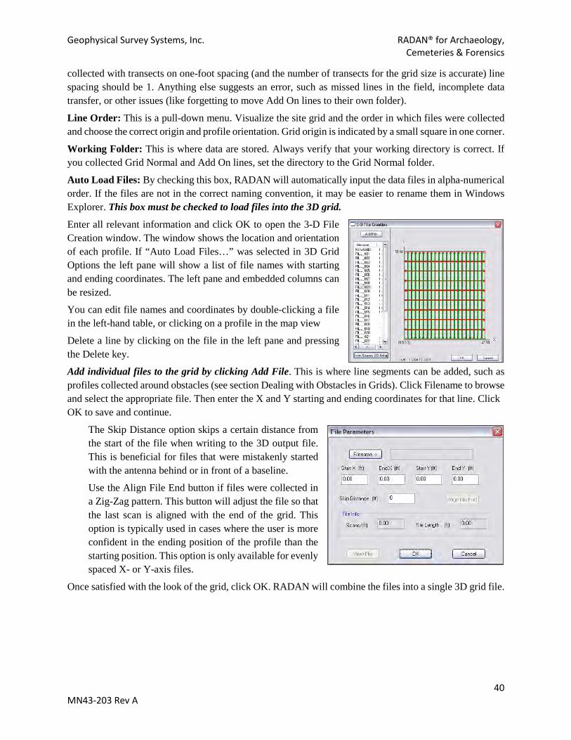
Geophysical Survey Systems, Inc. RADAN® for Archaeology, Cemeteries & Forensics
40 MN43-203 Rev A
collected with transects on one-foot spacing (and the number of transects for the grid size is accurate) line spacing should be 1. Anything else suggests an error, such as missed lines in the field, incomplete data transfer, or other issues (like forgetting to move Add On lines to their own folder).
Line Order: This is a pull-down menu. Visualize the site grid and the order in which files were collected and choose the correct origin and profile orientation. Grid origin is indicated by a small square in one corner.
Working Folder: This is where data are stored. Always verify that your working directory is correct. If you collected Grid Normal and Add On lines, set the directory to the Grid Normal folder.
Auto Load Files: By checking this box, RADAN will automatically input the data files in alpha-numerical order. If the files are not in the correct naming convention, it may be easier to rename them in Windows Explorer. This box must be checked to load files into the 3D grid.
Enter all relevant information and click OK to open the 3-D File Creation window. The window shows the location and orientation of each profile. If “Auto Load Files…” was selected in 3D Grid Options the left pane will show a list of file names with starting and ending coordinates. The left pane and embedded columns can be resized.
You can edit file names and coordinates by double-clicking a file in the left-hand table, or clicking on a profile in the map view
Delete a line by clicking on the file in the left pane and pressing the Delete key.
Add individual files to the grid by clicking Add File. This is where line segments can be added, such as profiles collected around obstacles (see section Dealing with Obstacles in Grids). Click Filename to browse and select the appropriate file. Then enter the X and Y starting and ending coordinates for that line. Click OK to save and continue.
The Skip Distance option skips a certain distance from the start of the file when writing to the 3D output file. This is beneficial for files that were mistakenly started with the antenna behind or in front of a baseline.
Use the Align File End button if files were collected in a Zig-Zag pattern. This button will adjust the file so that the last scan is aligned with the end of the grid. This option is typically used in cases where the user is more confident in the ending position of the profile than the starting position. This option is only available for evenly spaced X- or Y-axis files.
Once satisfied with the look of the grid, click OK. RADAN will combine the files into a single 3D grid file.

Geophysical Survey Systems, Inc. RADAN® for Archaeology, Cemeteries & Forensics
41 MN43-203 Rev A
4.2 DEALING WITH OBSTACLES IN GPR GRIDS (FOR MANUAL 3D ONLY)
Collect lines normally (forward or zig-zag). When you encounter an obstacle, stop your file. Then, move to the opposite baseline, face the obstacle, and collect a new profile from the baseline to the obstacle. Alternatively, you can start on the opposite side of the obstacle and collect a new profile that ends on the up-grid baseline. Good notes are critical for this procedure. The most important step is to know where a segment file starts or ends. This will make it easier to add it to a 3D grid.
When you download your data, make two folders in your working directory. One called “grid normal” lines and one called “add on” lines. Grid Normal lines are profiles that started on a baseline. Add On lines are profiles that were collected as segments to avoid obstacles. Place all Grid Normal lines into the Grid Normal folder. Put all your Add On lines in the Add On folder. When you build your 3D file in RADAN, use the grid normal directory for your working folder.
You will insert Add On lines during the 3D creation process (G – Assemble Data File – 3D File). Add your Grid Normal files, grid parameters, and other information. Press OK and you’ll see a 3D File Creation window with lines representing individual profiles (Red for X Axis, Green for Y Axis). In the upper left you’ll see Add File. Click this button for a File Parameters window, then click the Filename button to browse for an Add On line. Enter the Start X/ End X and Start Y/ End Y coordinates, then press OK.
For X Axis Add On lines the start/end Y field will be the same number. For Y Axis Add On lines the start/end X field will be the same number. You should already know the start or end coordinate for a X or Y axis line if you started or ended the file on one of your baselines. To figure out the other coordinates just subtract (or add) the file length from (or to) the known coordinate.

Geophysical Survey Systems, Inc. RADAN® for Archaeology, Cemeteries & Forensics
42 MN43-203 Rev A
In the 3D File Creation window, you should now see a blue line representing the location of the Add On line. Note the location of the arrowhead for Add On lines, and make sure it is oriented correctly.
4.3 CREATING A 3D BATCH OF FILES (THAT “PRE-PROCESSED”
LOOK) 3D Batch of Files creates a 3D Grid Batch file by combining individual data files (.DZT) that were collected on a grid. Files can be collected in the X direction only, Y direction only, or both X and Y directions.
Note that the batch file created will be a .BZX file and contain only the names of the files (and links to their location) to batch together. It will not be a data file (.DZT) of the files combined (unlike Create 3D File), so all files must remain in the same folder.
This 3D creation method will incorporate User Marks and other “pre-processing” steps used during collection. This will include auto or manual gains, filters (BR, IIR/FIR, Stacking, Etc.).
This method differs from Create 3D File in that 3D Batch of Files incorporates each profile’s .DZX file, thus including field parameters (Gain and Filters) to “pre-process” the data. I recommend using Create 3D File instead, so that files can be processed from raw data (instead of inheriting field gains/filters).
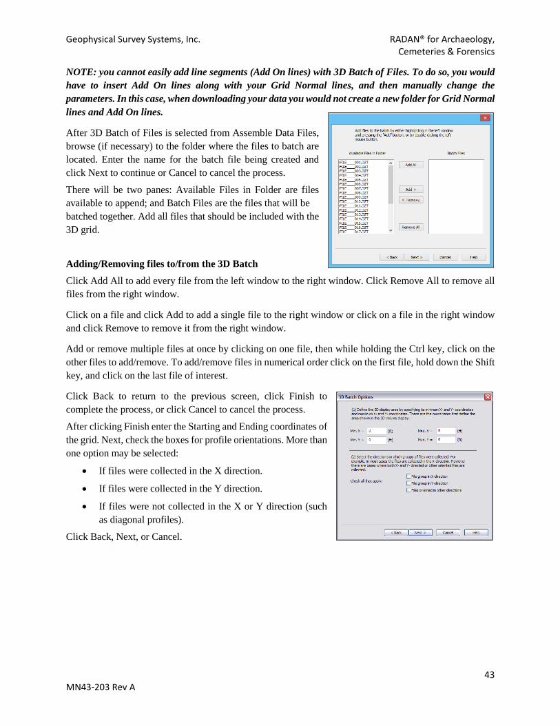
Geophysical Survey Systems, Inc. RADAN® for Archaeology, Cemeteries & Forensics
43 MN43-203 Rev A
NOTE: you cannot easily add line segments (Add On lines) with 3D Batch of Files. To do so, you would have to insert Add On lines along with your Grid Normal lines, and then manually change the parameters. In this case, when downloading your data you would not create a new folder for Grid Normal lines and Add On lines.
After 3D Batch of Files is selected from Assemble Data Files, browse (if necessary) to the folder where the files to batch are located. Enter the name for the batch file being created and click Next to continue or Cancel to cancel the process.
There will be two panes: Available Files in Folder are files available to append; and Batch Files are the files that will be batched together. Add all files that should be included with the 3D grid.
Adding/Removing files to/from the 3D Batch
Click Add All to add every file from the left window to the right window. Click Remove All to remove all files from the right window.
Click on a file and click Add to add a single file to the right window or click on a file in the right window and click Remove to remove it from the right window.
Add or remove multiple files at once by clicking on one file, then while holding the Ctrl key, click on the other files to add/remove. To add/remove files in numerical order click on the first file, hold down the Shift key, and click on the last file of interest.
Click Back to return to the previous screen, click Finish to complete the process, or click Cancel to cancel the process.
After clicking Finish enter the Starting and Ending coordinates of the grid. Next, check the boxes for profile orientations. More than one option may be selected:
• If files were collected in the X direction.
• If files were collected in the Y direction.
• If files were not collected in the X or Y direction (such as diagonal profiles).
Click Back, Next, or Cancel.
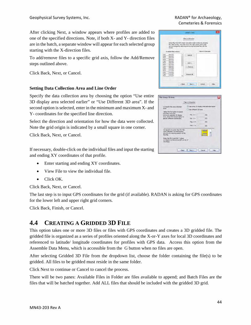
Geophysical Survey Systems, Inc. RADAN® for Archaeology, Cemeteries & Forensics
44 MN43-203 Rev A
After clicking Next, a window appears where profiles are added to one of the specified directions. Note, if both X- and Y- direction files are in the batch, a separate window will appear for each selected group starting with the X-direction files.
To add/remove files to a specific grid axis, follow the Add/Remove steps outlined above.
Click Back, Next, or Cancel.
Setting Data Collection Area and Line Order
Specify the data collection area by choosing the option “Use entire 3D display area selected earlier” or “Use Different 3D area”. If the second option is selected, enter in the minimum and maximum X- and Y- coordinates for the specified line direction.
Select the direction and orientation for how the data were collected. Note the grid origin is indicated by a small square in one corner.
Click Back, Next, or Cancel.
If necessary, double-click on the individual files and input the starting and ending XY coordinates of that profile.
• Enter starting and ending XY coordinates.
• View File to view the individual file.
• Click OK.
Click Back, Next, or Cancel.
The last step is to input GPS coordinates for the grid (if available). RADAN is asking for GPS coordinates for the lower left and upper right grid corners.
Click Back, Finish, or Cancel.
4.4 CREATING A GRIDDED 3D FILE This option takes one or more 3D files or files with GPS coordinates and creates a 3D gridded file. The gridded file is organized as a series of profiles oriented along the X-or-Y axes for local 3D coordinates and referenced to latitude/ longitude coordinates for profiles with GPS data. Access this option from the Assemble Data Menu, which is accessible from the G button when no files are open. After selecting Gridded 3D File from the dropdown list, choose the folder containing the file(s) to be gridded. All files to be gridded must reside in the same folder.
Click Next to continue or Cancel to cancel the process.
There will be two panes: Available Files in Folder are files available to append; and Batch Files are the files that will be batched together. Add ALL files that should be included with the gridded 3D grid.

Geophysical Survey Systems, Inc. RADAN® for Archaeology, Cemeteries & Forensics
45 MN43-203 Rev A
Adding/Removing files to/from the Gridded 3D File
Click Add All to add every file from the left window to the right window. Click Remove All to remove all files from the right window.
Click on a file and click Add to add a single file to the right window or click on a file in the right window and click Remove to remove it from the right window.
Add or remove multiple files at once by clicking on one file, then while holding the Ctrl key, click on the other files to add/remove. To add/remove files in numerical order click on the first file, hold down the Shift key, and click on the last file of interest.
When profiles are added a temporary file is created and the location view (above) shows locations of the GPS tracklines. Click Next to move to the next screen.
In the next window specify the dimensions of the 3D gridded area. By default, the area that appears encompasses all the data. There is an option to change the area to grid a subset of the data in this window. If there are no GPS coordinates the local grid area will be shown (feet or meters).
Click Next, then specify the distance between scans. Note that the gridded file size changes when the interval is changed.
Specify neighbor search information: Four is the default value for nearest neighbor. The neighbor distance should be at least the separation distance between profile lines.
Specify gridding method: Greater Distance Power reduces the interpolation impact of points farther away from a given node. By default, RADAN uses a Distance Power of 1, and 3 is the maximum.
Click Finish to create the Gridded 3D File. A status bar will indicate the progress of the file being created.

Geophysical Survey Systems, Inc. RADAN® for Archaeology, Cemeteries & Forensics
46 MN43-203 Rev A
Once the 3D gridded file is created, a prompt will appear to enter a file name. The file will open automatically after a name is provided. Note that Gridded 3D can create very large file sizes, especially when using a small interpolation value. Some files may be so large that the creation process fails. If this happens, consider changing a few parameters and check the export file size field before export.
Suggestions for collecting “gridded” data with a GPS plugged in. GPS-based data should be collected on the straightest transects possible. Collect individual profiles instead of a long “ribbon” of data across the project area. This will help with the 3D gridding process, and it will be easier to interpret individual profiles as opposed to one long, continuous file. Remember that GPR transect locations are only as good as the GPS resolution; if you want better resolution you’ll need a more accurate GPS. RADAN will not consider GPS elevation when displaying time slices, even if a Surface Normalization is performed. However, exported 2D Interactive points can be exported with these data in a separate column.
4.5 CREATING A SUPER 3D FILE This process combines multiple 3D Grids to create one “Super” 3D Grid. This will create a new file, containing all added grids, with the extension .DZT. Also created is a separate .s3d file, which contains the information used to create the output 3D file.
Individual 3D grids should be assigned local X and Y coordinates in 3D File Creation prior to creating a Super 3D grid.
To create a Super 3D File, click the RADAN G – Assemble Data File – Super 3D File. Next, enter a filename for the Super 3D file (.S3D) and then click Save to continue.
Click Add File to retrieve an already assembled 3D grid. RADAN will generate a warning, stating that all grids must have consistent Samples/Scan, Bits/Sample, Scans/Meter, Time Range, Dielectric, and Number of Channels. These parameters should be the same for all grids being combined. Keep this in mind when collecting field data, especially when returning to a field site for new data collection – the new data should have the same parameters as the original.
Click Filename to browse and retrieve a previously-created 3D grid. If necessary, enter the XY position for this grid. If starting XY coordinates were added during 3D File creation they will be automatically populated.
You can also Rotate, Flip Horizontally, and/or Flip Vertically, if needed. These settings should only be used to correct known errors.
Click OK, and if there are more grids to add repeat the process outlined above. If not, click OK.
4.6 ADDING GPS DATA TO A 3D GRID (AFTER DATA COLLECTION) A few notes for adding GPS coordinates. RADAN prefers latitude and longitude coordinates in decimal degrees. Use as many significant digits, (numbers to the right of the decimal point), as possible.
Open a 3D grid in RADAN. On the Home tab, click the Location button to open a window showing your grid and individual profile lines. Right-click inside the grid and select GPS Coords. Enter the latitude/longitude pairs for the specified grid corners. By default RADAN asks for the lower left corner (coordinate origin) and the upper right. You can only change the local coordinates for the second corner – RADAN requires the other corner to be the coordinate origin (lower left). Once the coordinates are entered
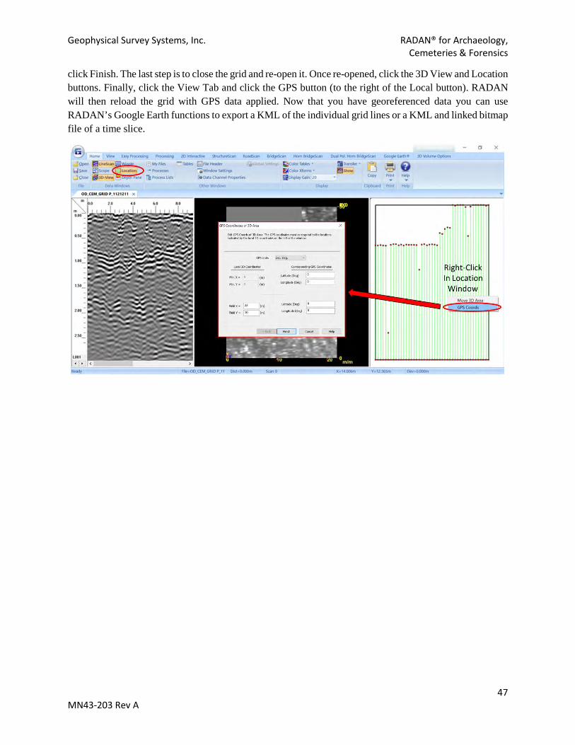
Geophysical Survey Systems, Inc. RADAN® for Archaeology, Cemeteries & Forensics
47 MN43-203 Rev A
click Finish. The last step is to close the grid and re-open it. Once re-opened, click the 3D View and Location buttons. Finally, click the View Tab and click the GPS button (to the right of the Local button). RADAN will then reload the grid with GPS data applied. Now that you have georeferenced data you can use RADAN’s Google Earth functions to export a KML of the individual grid lines or a KML and linked bitmap file of a time slice.

Geophysical Survey Systems, Inc. RADAN® for Archaeology, Cemeteries & Forensics
48 MN43-203 Rev A
SECTION 5: PROCESSING IMPACTS FOR 3D DATASETS
5.1 RANGE GAIN AND 3D DATA Range Gain is an important early processing step for 2D and 3D GPR data. This is especially true for 32-bit data that are assembled into a manually-created 3D grid (raw data, no gain). As noted above (Section 2.3) each Range Gain method can have a different impact on data interpretability. This is an important consideration for 3D datasets because relative amplitude differences provide contrast between targets and background information. If your goal is to make targets more obvious, a Range Gain that equalizes high and low amplitudes will make targets blend into the background. Or, perhaps your dataset contains large amplitude variations and you want to accentuate weaker amplitudes. You could apply a normalizing Range Gain (Auto or Adaptive) to bring down the high amplitudes and increase the weaker amplitudes, resulting in the enhancement of subtle targets that would otherwise be overshadowed by the strong amplitudes.
In the simple examples below, GPR survey at a golf course focused on re-locating historical sand traps (amorphous, high-amplitude, positive phase anomaly in images below). In this case, the targets/anomalies were more important than background soil information. Comparison of three different Range Gain methods (Auto, Adaptive, and Exponential) reveals which is most appropriate for the project requirements. An Auto Gain (left) ‘normalizes’ amplitudes along each profile to bring down the highs and accentuate the lows. The historical sand trap is visible but does not sharply contrast with the background. However, subtle landscape/soil anomalies are accentuated that may otherwise be overlooked. An Adaptive Gain (middle) achieves results like an Auto Gain, though the sand trap is more obvious at the expense of background soil information. Last, an Exponential Gain (right) is the best choice for displaying the sand trap (and utility lines) though the more subtle landscape/soil changes are not as obvious.
Auto Gain (13 Points, Horiz Tc 20) Adaptive Gain (Fast, 5 points) Exponential Gain (8 Points)
A more complicated dataset is shown below. These data were collected within the pauper section at a 19th-20th century cemetery. In the raw data examples, note the presence of numerous clearly-defined graves and the remnants of a historical road (not visible on the surface) running across the survey area. The amplitude differences between the shallow and deep slices are typical of raw datasets, where overall amplitudes drop off exponentially with increasing depth. A Range Gain could 1) improve the overall 3D interpretability by accentuating lower amplitudes, 2) slightly reducing higher amplitudes, and 3) applying a vertical normalization of the profile. This could reveal subtle information without blending important targets into the background. The amplitude variations between targets and background levels are quite variable, thus

Geophysical Survey Systems, Inc. RADAN® for Archaeology, Cemeteries & Forensics
49 MN43-203 Rev A
the chosen Range Gain method must retain subtle low amplitude information (background data) and low-to-mid amplitude data (historical path) without significantly reducing the amplitudes of the strongest targets (graves).
Shallow Raw Data showing former cemetery path Deeper Raw Data showing pauper graves
Data after Auto Gain (9 Pts, HorizTC 20). Left: historical cemetery path. Right: pauper graves.

Geophysical Survey Systems, Inc. RADAN® for Archaeology, Cemeteries & Forensics
50 MN43-203 Rev A
Data after Exponential Gain (9 Points). Left: historical cemetery path. Right: pauper graves.
Data after Adaptive Gain (Fast, 5 Points). Left: historical cemetery path. Right: pauper graves.
Note that Auto and Adaptive Gain downplay targets -- they are “lost in the background”. However, these gain methods can enhance weak patterning in background data (at the expense of targets).
5.2 TIME ZERO/POSITION CORRECTION AND NEAR-SURFACE 3D DATA
The Time Zero process sets the position of the ground surface based on the center of the Direct Wave’s first positive peak. This is a critical step in refining depth calibration (along with Migration – see below). However, important near-surface data exist within the Direct Wave and a Time Zero correction can remove them. I recommend investigating the shallow subsurface (0cm to ~10cm) prior to the Time Zero process (you might have to increase or decrease display gain). If there are useful data, like plow scars, paths/walkways, tire tracks, etc., consider exporting a time slice for later use – they could be removed by
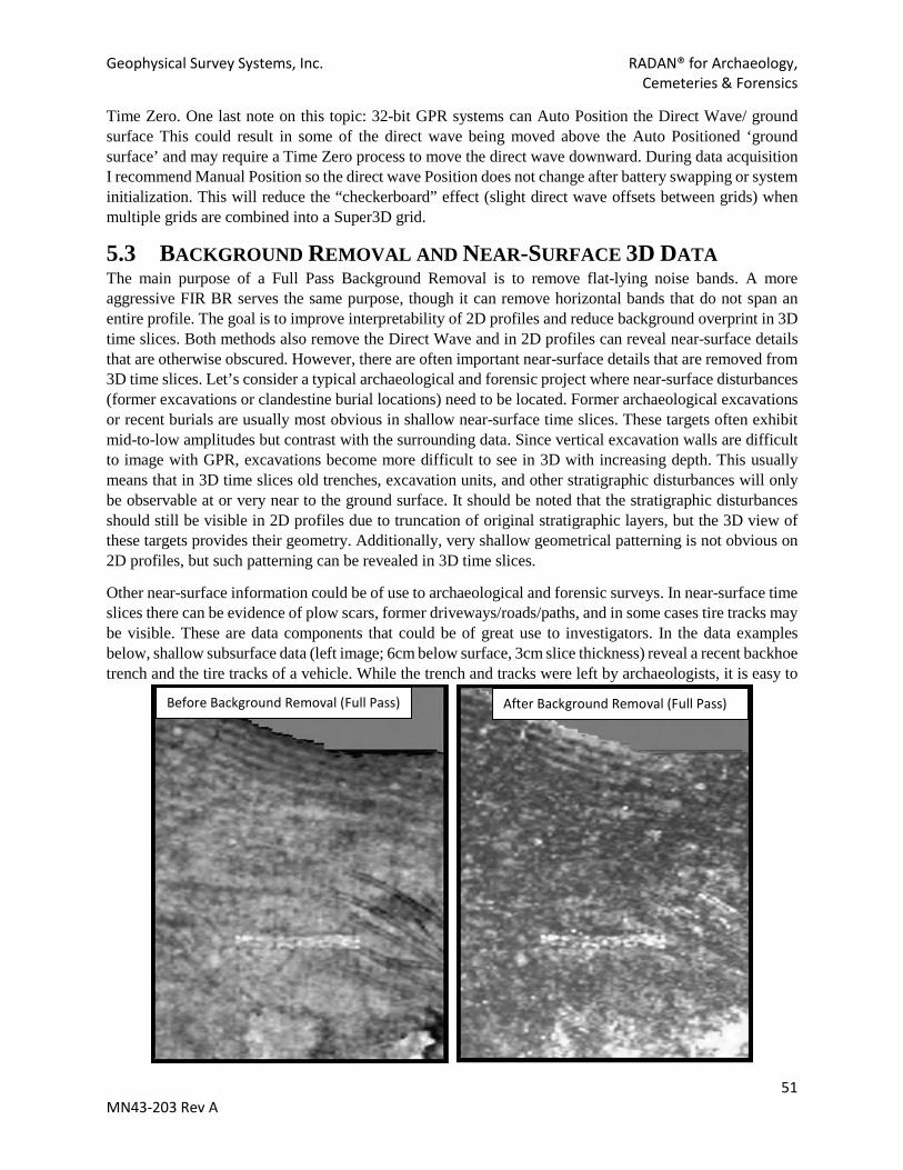
Geophysical Survey Systems, Inc. RADAN® for Archaeology, Cemeteries & Forensics
51 MN43-203 Rev A
Time Zero. One last note on this topic: 32-bit GPR systems can Auto Position the Direct Wave/ ground surface This could result in some of the direct wave being moved above the Auto Positioned ‘ground surface’ and may require a Time Zero process to move the direct wave downward. During data acquisition I recommend Manual Position so the direct wave Position does not change after battery swapping or system initialization. This will reduce the “checkerboard” effect (slight direct wave offsets between grids) when multiple grids are combined into a Super3D grid.
5.3 BACKGROUND REMOVAL AND NEAR-SURFACE 3D DATA The main purpose of a Full Pass Background Removal is to remove flat-lying noise bands. A more aggressive FIR BR serves the same purpose, though it can remove horizontal bands that do not span an entire profile. The goal is to improve interpretability of 2D profiles and reduce background overprint in 3D time slices. Both methods also remove the Direct Wave and in 2D profiles can reveal near-surface details that are otherwise obscured. However, there are often important near-surface details that are removed from 3D time slices. Let’s consider a typical archaeological and forensic project where near-surface disturbances (former excavations or clandestine burial locations) need to be located. Former archaeological excavations or recent burials are usually most obvious in shallow near-surface time slices. These targets often exhibit mid-to-low amplitudes but contrast with the surrounding data. Since vertical excavation walls are difficult to image with GPR, excavations become more difficult to see in 3D with increasing depth. This usually means that in 3D time slices old trenches, excavation units, and other stratigraphic disturbances will only be observable at or very near to the ground surface. It should be noted that the stratigraphic disturbances should still be visible in 2D profiles due to truncation of original stratigraphic layers, but the 3D view of these targets provides their geometry. Additionally, very shallow geometrical patterning is not obvious on 2D profiles, but such patterning can be revealed in 3D time slices.
Other near-surface information could be of use to archaeological and forensic surveys. In near-surface time slices there can be evidence of plow scars, former driveways/roads/paths, and in some cases tire tracks may be visible. These are data components that could be of great use to investigators. In the data examples below, shallow subsurface data (left image; 6cm below surface, 3cm slice thickness) reveal a recent backhoe trench and the tire tracks of a vehicle. While the trench and tracks were left by archaeologists, it is easy to
Before Background Removal (Full Pass) After Background Removal (Full Pass)
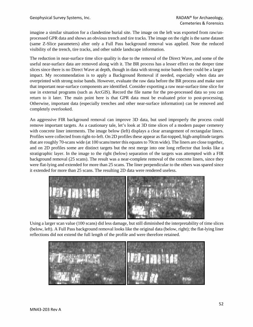
Geophysical Survey Systems, Inc. RADAN® for Archaeology, Cemeteries & Forensics
52 MN43-203 Rev A
imagine a similar situation for a clandestine burial site. The image on the left was exported from raw/un-processed GPR data and shows an obvious trench and tire tracks. The image on the right is the same dataset (same Z-Slice parameters) after only a Full Pass background removal was applied. Note the reduced visibility of the trench, tire tracks, and other subtle landscape information.
The reduction in near-surface time slice quality is due to the removal of the Direct Wave, and some of the useful near-surface data are removed along with it. The BR process has a lesser effect on the deeper time slices since there is no Direct Wave at depth, though in data with strong noise bands there could be a larger impact. My recommendation is to apply a Background Removal if needed, especially when data are overprinted with strong noise bands. However, evaluate the raw data before the BR process and make sure that important near-surface components are identified. Consider exporting a raw near-surface time slice for use in external programs (such as ArcGIS). Record the file name for the pre-processed data so you can return to it later. The main point here is that GPR data must be evaluated prior to post-processing. Otherwise, important data (especially trenches and other near-surface information) can be removed and completely overlooked.
An aggressive FIR background removal can improve 3D data, but used improperly the process could remove important targets. As a cautionary tale, let’s look at 3D time slices of a modern pauper cemetery with concrete liner interments. The image below (left) displays a clear arrangement of rectangular liners. Profiles were collected from right-to-left. On 2D profiles these appear as flat-topped, high-amplitude targets that are roughly 70-scans wide (at 100 scans/meter this equates to 70cm wide). The liners are close together, and on 2D profiles some are distinct targets but the rest merge into one long reflector that looks like a stratigraphic layer. In the image to the right (below) separation of the targets was attempted with a FIR background removal (25 scans). The result was a near-complete removal of the concrete liners, since they were flat-lying and extended for more than 25 scans. The liner perpendicular to the others was spared since it extended for more than 25 scans. The resulting 2D data were rendered useless.
Using a larger scan value (100 scans) did less damage, but still diminished the interpretability of time slices (below, left). A Full Pass background removal looks like the original data (below, right); the flat-lying liner reflections did not extend the full length of the profile and were therefore retained.
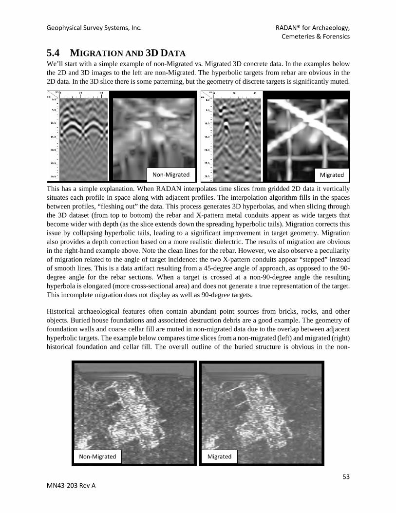
Geophysical Survey Systems, Inc. RADAN® for Archaeology, Cemeteries & Forensics
53 MN43-203 Rev A
5.4 MIGRATION AND 3D DATA We’ll start with a simple example of non-Migrated vs. Migrated 3D concrete data. In the examples below the 2D and 3D images to the left are non-Migrated. The hyperbolic targets from rebar are obvious in the 2D data. In the 3D slice there is some patterning, but the geometry of discrete targets is significantly muted.
This has a simple explanation. When RADAN interpolates time slices from gridded 2D data it vertically situates each profile in space along with adjacent profiles. The interpolation algorithm fills in the spaces between profiles, “fleshing out” the data. This process generates 3D hyperbolas, and when slicing through the 3D dataset (from top to bottom) the rebar and X-pattern metal conduits appear as wide targets that become wider with depth (as the slice extends down the spreading hyperbolic tails). Migration corrects this issue by collapsing hyperbolic tails, leading to a significant improvement in target geometry. Migration also provides a depth correction based on a more realistic dielectric. The results of migration are obvious in the right-hand example above. Note the clean lines for the rebar. However, we also observe a peculiarity of migration related to the angle of target incidence: the two X-pattern conduits appear “stepped” instead of smooth lines. This is a data artifact resulting from a 45-degree angle of approach, as opposed to the 90-degree angle for the rebar sections. When a target is crossed at a non-90-degree angle the resulting hyperbola is elongated (more cross-sectional area) and does not generate a true representation of the target. This incomplete migration does not display as well as 90-degree targets.
Historical archaeological features often contain abundant point sources from bricks, rocks, and other objects. Buried house foundations and associated destruction debris are a good example. The geometry of foundation walls and coarse cellar fill are muted in non-migrated data due to the overlap between adjacent hyperbolic targets. The example below compares time slices from a non-migrated (left) and migrated (right) historical foundation and cellar fill. The overall outline of the buried structure is obvious in the non-
Non-Migrated Migrated
Non-Migrated Migrated

Geophysical Survey Systems, Inc. RADAN® for Archaeology, Cemeteries & Forensics
54 MN43-203 Rev A
migrated data, but migration collapses hyperbolic tails and sharpens the outline of external and internal architectural components.
A more complex migration example is a cemetery dataset with numerous closely-spaced graves (see below). In this case, a 19th century pauper cemetery where space limitations required closely-spaced burials. These graves are obvious in 2D profiles as complex hyperbolic targets at a consistent depth (first). However, when viewed in 3D the individual interments are mostly visible but difficult to separate (second). This is because the hyperbolas and associated tails merge together to form long anomalous areas.
The 3D dataset reveals two anomalous high amplitude, grave-row-like features, but it is difficult to see discrete internal features. When migrated, the hyperbolic tails are collapsed (third) and there is better definition for each interment. In this case, a successful migration revealed two rows of very closely-spaced rectangular coffins (fourth).
One last point of interest. Some processes work well for 2D datasets and not for 3D data (and vice versa). The cemetery data are a perfect example of this conundrum. While Migration greatly improved the 3D geometry of graves, the migrated 2D profiles are now much more difficult to interpret without hyperbolic tails to denote point sources.
5.5 IIR FILTER AND 3D DATA IIR filtering is a powerful method for improving 2D profiles and offers a pathway for creative data manipulation. Additionally, the use of apply/reset for 2D data is handy for real-time evaluation of IIR impacts. In the 3D environment IIR filters provide similar benefits but cannot be evaluated in real-time. Therefore, this section demonstrates the impact of various high and low pass combinations on 3D datasets to facilitate proper use of IIR filters. We’ll start with a straightforward example of IIR (vertical) high and low pass filtering to restrict the frequency spectrum around an antenna’s central frequency. As discussed above (see Section 2.4) RF noise is ubiquitous and can be especially problematic in urban environments or close to the RF source. A simple use of IIR filtering would be removal of low frequency [LF] (radio) and high frequency [HF] (cellular) noise. In the example below, a 400MHz dataset was filtered with a conservative IIR filter (high pass: 200MHz; low pass: 700MHz). This wide frequency range improved the

Geophysical Survey Systems, Inc. RADAN® for Archaeology, Cemeteries & Forensics
55 MN43-203 Rev A
interpretability of 2D profiles (which exhibited LF banding and HF ‘fuzziness’); the impact on 3D time slices was minimal since only minor data components were removed.
A more aggressive IIR would not only remove HF/LF noise; it could remove LF/lower resolution frequencies and reduce clutter from HF/high resolution components. The example below shows the results of an IIR filter with HP300 and LP600 (8 poles). The slice on the right exhibits clearer geometrical features (walls, circular feature near center of structure) with a normalization in overall amplitudes. This is mostly due to removal of lower frequencies that cause ‘ringing’ and a blurring of target edges from LF components.
Now for some aggressive and creative filtering methods to highlight specific data components. The following examples heavily impacted 3D slices and 2D profiles and were used to improve 3D data at the expense of 2D interpretability. The first example (below) applied an IIR filter (8 poles) to discard all frequencies lower than the antenna’s central frequency (350MHz). Note the similarity to an IIR with HP300 and LP600. This suggests that the LF data components below 350-300Mhz are muting the geometry of targets of interest, while the HF frequencies are producing consistent and refined results despite a LP increase to 700MHz.
Before IIR Filter IIR Filter: HP300 LP600 (8 poles)
Before IIR Filter IIR Filter: HP200 LP700 (8 poles)
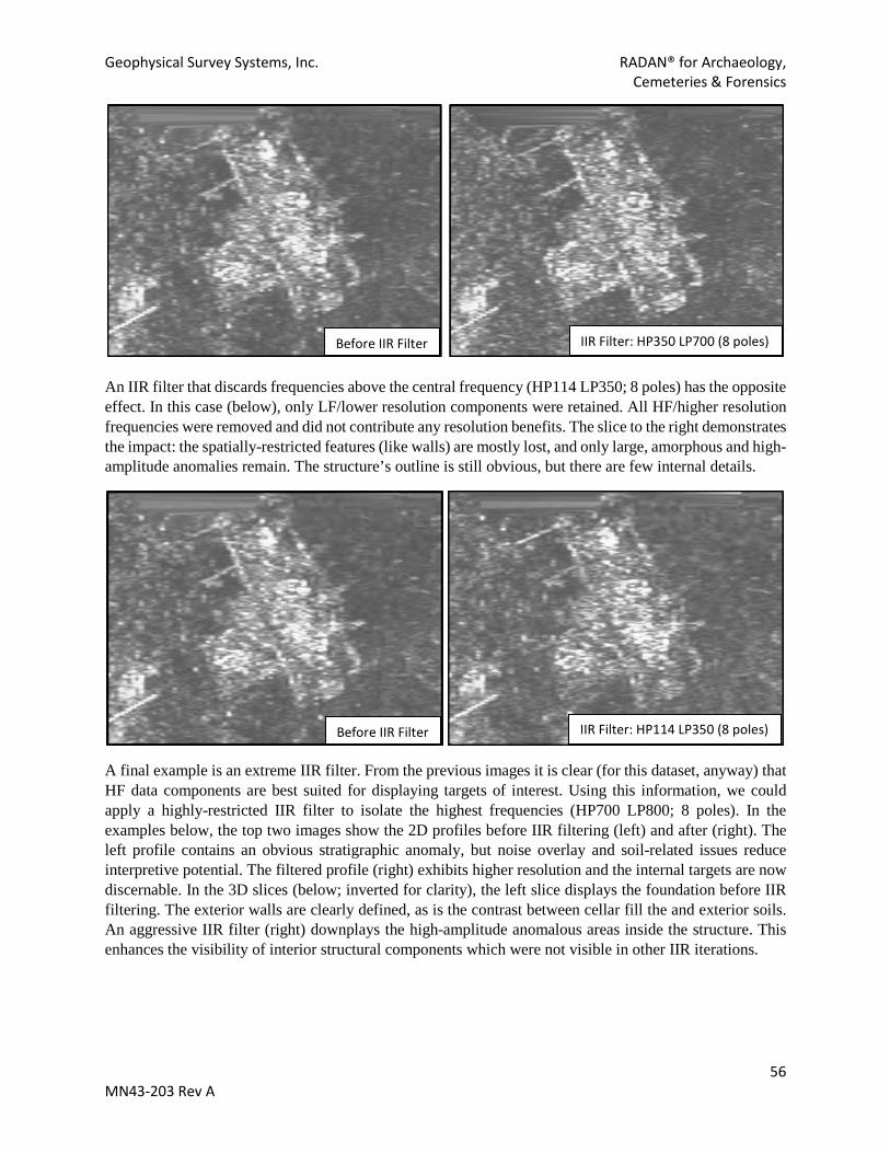
Geophysical Survey Systems, Inc. RADAN® for Archaeology, Cemeteries & Forensics
56 MN43-203 Rev A
An IIR filter that discards frequencies above the central frequency (HP114 LP350; 8 poles) has the opposite effect. In this case (below), only LF/lower resolution components were retained. All HF/higher resolution frequencies were removed and did not contribute any resolution benefits. The slice to the right demonstrates the impact: the spatially-restricted features (like walls) are mostly lost, and only large, amorphous and high-amplitude anomalies remain. The structure’s outline is still obvious, but there are few internal details.
A final example is an extreme IIR filter. From the previous images it is clear (for this dataset, anyway) that HF data components are best suited for displaying targets of interest. Using this information, we could apply a highly-restricted IIR filter to isolate the highest frequencies (HP700 LP800; 8 poles). In the examples below, the top two images show the 2D profiles before IIR filtering (left) and after (right). The left profile contains an obvious stratigraphic anomaly, but noise overlay and soil-related issues reduce interpretive potential. The filtered profile (right) exhibits higher resolution and the internal targets are now discernable. In the 3D slices (below; inverted for clarity), the left slice displays the foundation before IIR filtering. The exterior walls are clearly defined, as is the contrast between cellar fill the and exterior soils. An aggressive IIR filter (right) downplays the high-amplitude anomalous areas inside the structure. This enhances the visibility of interior structural components which were not visible in other IIR iterations.
Before IIR Filter IIR Filter: HP350 LP700 (8 poles)
Before IIR Filter IIR Filter: HP114 LP350 (8 poles)

Geophysical Survey Systems, Inc. RADAN® for Archaeology, Cemeteries & Forensics
57 MN43-203 Rev A
5.6 MATHEMATICAL FUNCTIONS AND 3D DATA Mathematical functions are not commonly applied to 2D or 3D GPR data, but in certain cases they can be useful for accentuating 3D details. As detailed above (see section on math functions and 2D data), of the available Mathematical functions only differentiate and integrate are viable options. Differentiate will preferentially highlight the largest amplitude changes at the expense of minor vertical amplitude differences. This will accentuate large changes and ‘mute’ smaller changes. Integrate has the opposite effect: it is a cumulative function that enhances amplitudes much like a range gain process. The impact of these two math functions is more obvious in 2D profiles, but they could highlight different 3D data components and may prove useful for 3D visualization. You might find that IIR filtering is a better option, though math functions do not clip the frequency spectrum and may work best without applying an IIR filter. Mathematical functions should be used towards the end of post-processing, since they can reduce 2D interpretability. The most significant issue with math functions is time shifts. Differentiate shifts targets and layers up and can cause one or more nanoseconds of vertical displacement. This can be problematic if depth to targets is a critical variable. Integrate does not create time shifts.
2D Profile: Before IIR Filter 2D Profile: IIR Filter: HP700 LP800 (8 poles)
3D Slice: Before IIR Filter 3D Slice: IIR Filter: HP700 LP800 (8 poles)

Geophysical Survey Systems, Inc. RADAN® for Archaeology, Cemeteries & Forensics
58 MN43-203 Rev A
For this discussion we’ll start with data from the IIR and 3D section (Section 5.5) to evaluate the Differentiate function. The final examples from IIR and 3D used aggressive HP/LP filtering to refine the geometry of a buried structure and cellar fill. We’ll see if we can achieve the same results with Differentiate. In the images to the right the top image displays a historical structure with complex internal fill, geometrical outline, and internal walls. Prior to the IIR filter the structure’s internal details were masked by high amplitudes (Section 5.5). These data were processed with an aggressive IIR filter (HP700, LP800) to retain only the highest frequencies (highest resolution data components).
The central image was processed with migration (to clean up the point sources) and a Differentiate filter. The overall data amplitudes were reduced, allowing internal structural details to stand out against fill units. Most of the weaker amplitude targets outside the structure are less obvious than they are in the top image, and the structure’s outline isn’t as well defined.
In this case, a Differentiate filter improved the 3D data, but there are noticeable data losses in areas of mid-to-low amplitudes. This is because the Differentiate filter moves vertically through the data, and small changes are even further reduced. Another important consideration is the time shifts that occur with Differentiate, which makes targets shallower than they were before the filter was applied.
The bottom image was processed with Migration, Differentiate, and then an aggressive IIR filter (HP600 LP700). This dataset is cleaner than just using an aggressive IIR filter. However, the 2D dataset is now very difficult to interpret, and there are time shifts.
To evaluate the Integrate function we’ll use examples from the section on Range Gain and 3D data. Since Integrate generates data that can look like the results of a Range Gain, we’ll see if we can improve 3D data by applying Integrate instead of a Range Gain. It should be noted that Integrate is not a substitute for a Range Gain – it does not vertically equalize amplitudes, but instead adds values cumulatively. It should therefore only be applied after an actual range gain. In the examples below, a dataset is shown before an Integrate function (left) and after (right). These were SIR3000-based data and had inherited field gain. Note that there is very little difference between the pre- and post-Integrate datasets. This is due to the shallow depths of the features. The cumulative effects of an Integrate function are much more pronounced with depth, since there are more stacked amplitude variations as depth increases. Mathematical functions are an interesting addition to 3D data processing, but they can produce unexpected data artifacts and reduce the
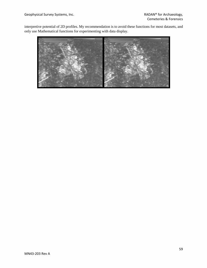
Geophysical Survey Systems, Inc. RADAN® for Archaeology, Cemeteries & Forensics
59 MN43-203 Rev A
interpretive potential of 2D profiles. My recommendation is to avoid these functions for most datasets, and only use Mathematical functions for experimenting with data display.
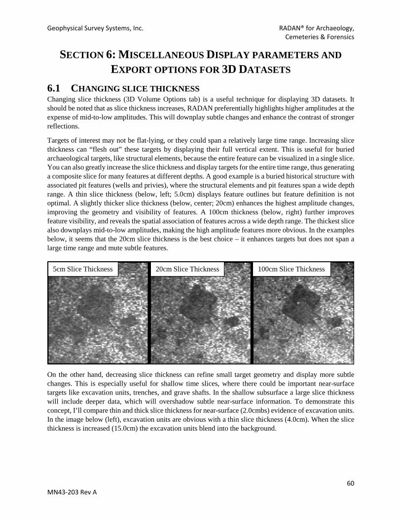
Geophysical Survey Systems, Inc. RADAN® for Archaeology, Cemeteries & Forensics
60 MN43-203 Rev A
SECTION 6: MISCELLANEOUS DISPLAY PARAMETERS AND EXPORT OPTIONS FOR 3D DATASETS
6.1 CHANGING SLICE THICKNESS Changing slice thickness (3D Volume Options tab) is a useful technique for displaying 3D datasets. It should be noted that as slice thickness increases, RADAN preferentially highlights higher amplitudes at the expense of mid-to-low amplitudes. This will downplay subtle changes and enhance the contrast of stronger reflections.
Targets of interest may not be flat-lying, or they could span a relatively large time range. Increasing slice thickness can “flesh out” these targets by displaying their full vertical extent. This is useful for buried archaeological targets, like structural elements, because the entire feature can be visualized in a single slice. You can also greatly increase the slice thickness and display targets for the entire time range, thus generating a composite slice for many features at different depths. A good example is a buried historical structure with associated pit features (wells and privies), where the structural elements and pit features span a wide depth range. A thin slice thickness (below, left; 5.0cm) displays feature outlines but feature definition is not optimal. A slightly thicker slice thickness (below, center; 20cm) enhances the highest amplitude changes, improving the geometry and visibility of features. A 100cm thickness (below, right) further improves feature visibility, and reveals the spatial association of features across a wide depth range. The thickest slice also downplays mid-to-low amplitudes, making the high amplitude features more obvious. In the examples below, it seems that the 20cm slice thickness is the best choice – it enhances targets but does not span a large time range and mute subtle features.
On the other hand, decreasing slice thickness can refine small target geometry and display more subtle changes. This is especially useful for shallow time slices, where there could be important near-surface targets like excavation units, trenches, and grave shafts. In the shallow subsurface a large slice thickness will include deeper data, which will overshadow subtle near-surface information. To demonstrate this concept, I’ll compare thin and thick slice thickness for near-surface (2.0cmbs) evidence of excavation units. In the image below (left), excavation units are obvious with a thin slice thickness (4.0cm). When the slice thickness is increased (15.0cm) the excavation units blend into the background.
5cm Slice Thickness 20cm Slice Thickness 100cm Slice Thickness

Geophysical Survey Systems, Inc. RADAN® for Archaeology, Cemeteries & Forensics
61 MN43-203 Rev A
6.2 USING MAX VS RMS (3D VOLUME OPTIONS WINDOW) As slice thickness increases, RADAN averages a larger depth window and preferentially displays higher amplitudes while downplaying mid-to-low amplitudes (see above: Changing Slice Thickness). This can lead to gain oversaturation in areas of high reflection coefficients. RADAN’s 3D Volume Options window provides two options for viewing amplitudes: Max and RMS. Max will display amplitudes without clipping or normalizing. The RMS (Root Mean Square) option squares all data values, calculates the mean value, and displays data amplitudes based on the square root of the mean value. In general, the RMS option will reduce higher amplitudes relative to lower amplitudes and created more normalized amplitudes across a dataset. The RMS option is most effective when applied to larger slice thicknesses, due to variations in amplitudes with depth and
the tendency for RADAN to highlight higher amplitudes with increasing slice thickness. This can be demonstrated with a few data examples. The two images below are identical (same depth, 15cm
Near-Surface: 4cm Slice Thickness Near-Surface: 15cm Slice Thickness
Max with 15cm Slice Thickness RMS with 15cm Slice Thickness

Geophysical Survey Systems, Inc. RADAN® for Archaeology, Cemeteries & Forensics
62 MN43-203 Rev A
slice thickness), except the left example is displayed with Max values and the right example uses the RMS option. The example to the right required an increase in display gain, but otherwise looks identical to the example on the left.
With increased slice thickness the effect of RMS is more pronounced. The two images below are identical (same depth, 60cm Slice Thickness) but the image to the left is displayed with Max, and the image to the right uses the RMS option. The image on the right exhibits normalized amplitudes and reveals more detail inside the building footprint because mid-to-low amplitudes are not overshadowed by high amplitude areas.
6.3 REDUCING “CHECKERBOARDING” IN SUPER 3D (TABLES PANE) If 3D data were collected across multiple days, or batteries were swapped out in the middle of a grid, you could see a “checkerboard” effect in near-surface slices. This is because the position of Time Zero shifted, most likely due to Auto Position on your control unit (SIR3000, SIR4000, UtilityScan DF/HS), or Auto Gain was enabled (especially SIR3000-based data). For 32-bit 3D data created with .DZX files (3D Batch of Files) this could also be related to Auto Gains during fieldwork. When collecting gridded 3D datasets, I recommend setting Position and Gain to Manual (if available) before data collection. This will prevent slight time shifts and amplitude shifts. However, there can still be amplitude/gain and time zero offsets between adjacent Super3D grids that are related to environmental factors (e.g. a rainstorm).
Time offsets can be repaired by applying a Time Zero correction to a grid before it is added to a Super3D grid. Gain variations between grids can be more difficult to handle. For 16-bit data, you can apply a Gain Restoration (Processing Tab) to reduce gain issues. For 32-bit data, Gain Restoration will only work when the .DZX was applied during 3D grid creation (3D Batch of Files). You can get around these issues by turning on the Tables Pane (Home Tab) and selecting the 3DSubArea Options tab. Look for the Loc. 3D Gain column header, and you’ll see local gain set to 0 for each grid.
Max with 60cm Slice Thickness RMS with 60cm Slice Thickness

Geophysical Survey Systems, Inc. RADAN® for Archaeology, Cemeteries & Forensics
63 MN43-203 Rev A
You can use Loc. 3D Gain to increase or decrease the overall gain for one or more grids. This will help reduce the ‘checkerboarding’ effect from amplitude variations between grids. In the Super3D examples below, the amplitudes for one grid are lower than the other three (below, left). Using Loc. 3D Gain the local gain of the problem grid was increased to 6 (below, right), and the grid now blends in with the other three.
6.4 REMOVING THE XY TEXT FROM THE LOWER LEFT GRID ORIGIN You might have noticed a X/Y text overprint on exported 3D slice images (lower left corner). RADAN offers no option to remove the letters, but there is an easy workaround. The image to the right shows a typical time slice with the X/Y text. To remove the text, first hold down the X key on your keyboard, then press your keyboard’s up arrow 10 times. The 3D slice will stretch in the X direction. Next, repeat the process using the Y key on your keyboard. Use your mouse wheel to zoom out, and you will no longer see the X/Y text. You can repeat the process if the text is still visible. The process will be reversed if you click the Reset view button (3D Volume Options tab).
Geophysical Survey Systems, Inc. RADAN® for Archaeology, Cemeteries & Forensics
64 MN43-203 Rev A
6.5 EXPORTING 3D DATA FROM RADAN 7 RADAN offers multiple options for exporting 3D data. The most common method is to export time slice images for use in other programs. Other choices include exporting time slices as KML files (GPS data required) and exporting a XYZ point cloud for a given slice depth/thickness.
To export time slice images, set desired parameters on the 3D Volume Options tab (depth, thickness, display gain, etc.), then go to G – Export – Custom Image Export. Choose the image format (.jpg, .bmp, .png), select 3D View window, and for Image Size choose Current Window. Name the export file, and choose a save directory. I recommend a standardized naming convention for exported slices – this will help keep track of the export parameters. I name my exported slices as follows: 50cmPM20cm. This tells me that the slice depth was 50cm, and the slice thickness was 20cm. This reads as 50cm Plus or Minus (PM) 20cm. A consistent naming convention will be quite helpful when importing slices to a GIS program. You can also export the Location window using this option – just choose Location instead of 3D View Window.
For certain datasets it is critical that a near-surface time slice is exported prior to Time Zero correction and Background Removal (see section Background Removal and 3D Datasets). It is assumed that data within the direct wave are unusable, but experience has shown that there are important details in the near-surface slices that can be clipped off with a position correction. These details include near-surface components of trenches, grave shafts (from formal graves and clandestine burials), older excavation units, and surface features such as walkways and paths. With this in mind, export a near-surface slice prior to applying a Time Zero and Background Removal (but remember – you’ll probably have to increase display gain).
Time slices can be exported as XYZ text files for display and interpolation in other programs (ArcGIS, Surfer, AutoCAD, etc.). This method exports XYZ points for a given slice depth and slice thickness. To access this option, click the G – Export -- Export 3D Slice as ASCII File. You’ll then see a Save Slice Data window asking you to Save X, Y, or Z Slice as an ASCII CSV File. Click the button for Z to export the time slice data. Name the file (use consistent naming convention as mentioned above) and choose a save directory. The export table will not have column headers. The exported columns are: Field 1: X Coordinate; Field 2: Y Coordinate; Field 3: Depth; Field 4: Amplitude. Note that areas of interpolation (across large gaps in 3D data coverage) will usually have an Amplitude value of 0. If you want to export the full amplitude range for 3D points, open 3D Window Options and turn off Background Removal (under Z-Slice Processing).
3D slices can also be exported as KML files (GPS data required) for use in Google Earth (other programs can convert KML to different GIS formats). Your computer must have a NVIDIA GPU to use this export option, and to open the exported files Google Earth must be installed. To use this method, set desired parameters on the 3D Volume Options tab (depth, thickness, display gain, etc.), the go to G – Export – Z-Slice Google Earth. Name the file and choose a save directory. Using Windows Explorer, navigate to the exported KML file. You’ll see that there is a KML file and a .bmp file with the same name. The KML file contains georeferencing information, and the .BMP contains the exported slice image. Double-click the KML, and the slice will open in Google Earth.

Geophysical Survey Systems, Inc. RADAN® for Archaeology, Cemeteries & Forensics
65 MN43-203 Rev A
6.6 “RUBBERSHEETING” 3D DATA IN RADAN YOU EXPECTED THIS: AND YOU GOT THIS….
Gridded GPR datasets might inherit unavoidable along-line offsets that lead to striping in time slices and offsets in target positioning between adjacent profiles. These offsets are derived from numerous field issues, including localized topographic irregularities and more commonly from distance-encoder errors or improper encoder calibration. These errors may also come from encoder skipping/sliding in wet or snowy conditions, or failure of the encoder to rotate when passing over holes or trenches. In the worst-case scenario, improper layout of geophysical grids may lead to skewed data. These issues are extremely frustrating and can lead to reduced interpretability for GPR time slices.
Some of the above-stated errors are avoidable if a field worker accurately calibrates their distance-encoding wheel and pays attention to ground conditions. Unfortunately, the other sources of error are usually unavoidable. To this end, when post-processing 3D grids in RADAN 7 it may be necessary to “rubbersheet” certain profiles to preserve the geometry of targets in time slices. Rubbersheeting stretches a GPR profile to a certain length to account for compression/stretching of the profile due to encoder/distance issues. For instance, along a 20m-long transect the profile length may read 18.7m although the operator moved the antenna from 0.0m to 20.0m. In this case, the GPR antenna traveled the desired distance but one or more variables caused the recorded distance to be incorrect. While rubbersheeting helps to fix between-line offsets, it is not creating new data. Note: the method outlined below is most effective when gridded profiles started and ended exactly on baselines (another component of detailed 3D collection).
First, create a 3D grid using the G – Assemble Data File – 3D File. [See above sections for more information on manually creating 3D datasets.]
Open the grid in RADAN, and on the Home Tab press the Location button.

Geophysical Survey Systems, Inc. RADAN® for Archaeology, Cemeteries & Forensics
66 MN43-203 Rev A
To the right is a location view from bidirectional (or zigzag) collection. Notice the extreme offset between profiles in opposing directions (~1.1m). In your data, you might see one or more lines that do not reach the upper or lower grid baseline, or perhaps all your lines exhibit offsets. Some degree of rubbersheeting in necessary here, since the GPR time slices will have considerable striping and the geometry of targets will be muted (if not obliterated).
To fix these offsets, start by opening the Tables Pane (Home Tab – Tables button). Then, click Profiles on the bottom of the Tables Pane.
For this example grid, the dimensions are 20m (Y) by 20m (X), with only Y lines collected in bidirectional/ zigzag mode. The first three grid-north trending lines stopped at an obstacle, and a short section was added grid north of the third line. Notice in the tables pane that all the odd-numbered profiles (5,7,9,11, etc.) have X St (m) [X coordinate start] and X End (m) [X coordinate end] separated by 20m. This is because there is only a single x coordinate for each gridded profile (the coordinates only change in Y axis direction). The distance offset is obvious in the Y coordinates. For example, Profile 5 (a grid south oriented profile) starts at Y 5546.100 and ends at Y 5565.00. There is a 1.1m offset, and the coordinates should start at Y 5545.00 (the grid south baseline). To fix this issue, we’ll have to rubbersheet Profile 5 to stretch it the full 20m.
Click the Edit 3D Position button on the right side of the Profiles Pane and you’ll see an Edit Profile Coords window. First, uncheck the Fixed Length box. Next, change the Start Y (m) value to the correct baseline coordinates. In this case, the correct Start Y (m) value would be 5545.0.
As a result, the 3D length of Profile 5 has been stretched from the upper to lower baselines (20m instead of 18.9m).
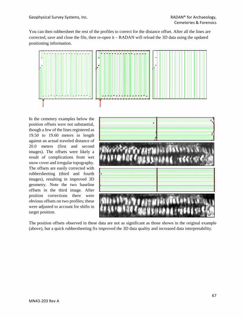
Geophysical Survey Systems, Inc. RADAN® for Archaeology, Cemeteries & Forensics
67 MN43-203 Rev A
You can then rubbersheet the rest of the profiles to correct for the distance offset. After all the lines are corrected, save and close the file, then re-open it – RADAN will reload the 3D data using the updated positioning information.
In the cemetery examples below the position offsets were not substantial, though a few of the lines registered as 19.50 to 19.60 meters in length against an actual traveled distance of 20.0 meters (first and second images). The offsets were likely a result of complications from wet snow cover and irregular topography. The offsets are easily corrected with rubbersheeting (third and fourth images), resulting in improved 3D geometry. Note the two baseline offsets in the third image. After position corrections there were obvious offsets on two profiles; these were adjusted to account for shifts in target position. The position offsets observed in these data are not as significant as those shown in the original example (above), but a quick rubbersheeting fix improved the 3D data quality and increased data interpretability.

Geophysical Survey Systems, Inc. RADAN® for Archaeology, Cemeteries & Forensics
68 MN43-203 Rev A
CONCLUDING REMARKS RADAN 7 is a powerful post-processing solution for GSSI GPR data. As there are many options available, and some have similar and overlapping functionality, a guide to their implementation and best use scenarios is essential. Furthermore, archaeological, forensic, and cemetery investigations are among the more difficult of GPR applications due to the variable nature of targets and survey environments. This guide is by no means an exhaustive treatment of post-processing such datasets, but it is hoped that the descriptions, examples, and recommendations herein have helped you to implement effectively the RADAN 7 processes and to understand when (and when not) to use them.
As a final note, this guide is a work in progress. As GPR technology develops, and RADAN 7 features are modified and enhanced, updates will be necessary. Check our website (www.geophysical.com) for future revisions to this document. Additionally, do not forget to check for Radan 7 updates (through our website or through RADAN) – we are constantly adding features and refining existing functionality.
As always, for RADAN 7 assistance please feel free to call our Technical Support team at 603-893-1109. Or, email the GSSI Training Team at [email protected].
Now, get out there and zap stuff with GPR -- and have fun doing it!
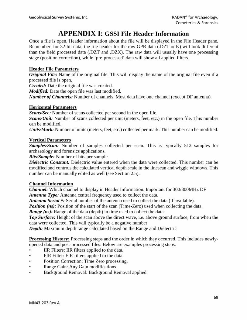
Geophysical Survey Systems, Inc. RADAN® for Archaeology, Cemeteries & Forensics
69 MN43-203 Rev A
APPENDIX I: GSSI File Header Information Once a file is open, Header information about the file will be displayed in the File Header pane. Remember: for 32-bit data, the file header for the raw GPR data (.DZT only) will look different than the field processed data (.DZT and .DZX). The raw data will usually have one processing stage (position correction), while ‘pre-processed’ data will show all applied filters. Header File Parameters Original File: Name of the original file. This will display the name of the original file even if a processed file is open. Created: Date the original file was created. Modified: Date the open file was last modified. Number of Channels: Number of channels. Most data have one channel (except DF antenna).
Horizontal Parameters Scans/Sec: Number of scans collected per second in the open file. Scans/Unit: Number of scans collected per unit (meters, feet, etc.) in the open file. This number can be modified. Units/Mark: Number of units (meters, feet, etc.) collected per mark. This number can be modified.
Vertical Parameters Samples/Scan: Number of samples collected per scan. This is typically 512 samples for archaeology and forensics applications. Bits/Sample: Number of bits per sample. Dielectric Constant: Dielectric value entered when the data were collected. This number can be modified and controls the calculated vertical depth scale in the linescan and wiggle windows. This number can be manually edited as well (see Section 2.5).
Channel Information Channel: Which channel to display in Header Information. Important for 300/800MHz DF Antenna Type: Antenna central frequency used to collect the data. Antenna Serial #: Serial number of the antenna used to collect the data (if available). Position (ns): Position of the start of the scan (Time-Zero) used when collecting the data. Range (ns): Range of the data (depth) in time used to collect the data. Top Surface: Height of the scan above the direct wave, i.e. above ground surface, from when the data were collected. This will typically be a negative number. Depth: Maximum depth range calculated based on the Range and Dielectric
Processing History: Processing steps and the order in which they occurred. This includes newly-opened data and post-processed files. Below are examples processing steps. • IIR Filters: IIR filters applied to the data. • FIR Filter: FIR filters applied to the data. • Position Correction: Time Zero processing. • Range Gain: Any Gain modifications. • Background Removal: Background Removal applied.
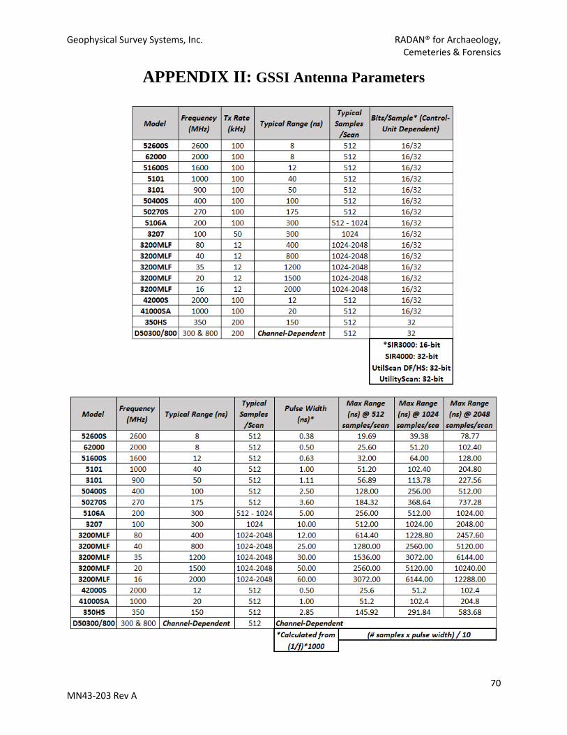
Geophysical Survey Systems, Inc. RADAN® for Archaeology, Cemeteries & Forensics
70 MN43-203 Rev A
APPENDIX II: GSSI Antenna Parameters