rAD~A27 853AD:

PL-TR-91 -3009 DTICELECTE

FinaReport TWENTY FIRST CENTURYfor the period

February 1989 o PROPULSION CONCEPTJuly 1990

May 1991 Author: Veritay Technology, Inc.R.L. Talley 4845 Millersport Highway

East Amherst NY 14051...

F04611-89-C-0023

Approved for Public Release

Distribution Is unlimited. The OL-AC PL Technical Services Office hasreviewed this report and it is relea3eable to the National Technical

Information Service, where It will be available to the general public,including foreign nationals.

Prepared for the: Phillips LaboratoryAir Force Systems CommandPropulsion Directorate

91-04377 Edwards AFB CA 93523-5000

91 7 5OZi

NOTICE

When U. S. Government drawings, specifications, or other data are used for any purpose oth-er than a definitely related Government procurement operation, the fact that theGovernment may have formulated, furnished, or in any way supplied the said drawings, speci-fications, or other data, is not to be regarded by implication or otherwise, or in any waylicensing the holder or any other person or corporation, or conveying any rights or permissionto manufacture, use or sell any patented invention that may be related thereto.

FOREWORD

This final report was submitted by Veritay Technology, Inc., East Amherst NY, on completionof Small Business Inovation Research (SBIR) Contract F04611-89-C-0023 with the OL--ACPhillips Laboratory (AFSC), Edwards AFB CA. PL Project Manager was Dr. Frank Mead.

This report has been reviewed and is approved for release and distribution in accordance withthe distribution statement on the cover and on the DD Form 1473.

FRANKLIN B. MEAD, JR. 41 STEPHEN L. ROD(RRSProject Manager Chief, Emerging Technologies Branch

FOR THE COMMANDER

DAVID W. LEWIS, MAJOR, USAFActing DirectorFundamental Technologies Division

REPORT DOCUMENTATION PAGE For ApprNo.ved.O1

Public reporlhgn bu ef' C' thIt £iItctiofl of iflfoiwtiomis esm t to a, wage hour Petrwie , ? i'.ncluding the fumn. fo reuw.i unt cin ,-atchuing *uurthurg data souri.9tPthleueg in u weu'auug 111. d.1. needed, anid conplet-rig en ~chqI cheic fufm un. Send coriiments revafsiir¶ Flu bveden esilmait or itit ootN. atpsc of this

1. ll~iton l Ofci OPatior'. io.Iducing suqgletuons lot uedw(~n9 this burcier to, Washi~ngtonl Herdd~uarteus Seri'ces, Dueftfdofalt for Inuformation, Opsuat4*r and Re~iorts, ,1 hi ffts oDb.mo Hiugh. V, Sijte I12C4. Arlington. VA 22.a0224302. is'.d to theu ofice of Maiugaqenmn ofie Budget, PaptrveoAt Rediuction Proleci (0704-0 SSI. Washington. DC 05S03.

~.AGkNCY USE ONLY (Leave blak .RPRT DATE 3. 11EPORT TYPE AND DATIES COVEREDj ay1991 I Final report from 7 Feb 89-7 Jul 90

4. TITLE AND SUBTITLE 5. FUNDING NUMBERSTWENTY FIRST CENTURY PROPULSION CONCEPT (U) PE 65502?

PR 3058____ ___ ___ ___ ___ ___ ____ ___ ___ ___ ___ ___ ___TA 0026

S. AUTHOR(S) C F04611-89-C.*0023

1Robert L. Talley WlS354

7. PERFORMING ORGANIZ'ATION NAME(S) AND ADDRESS(ES) 8. PERFORMING ORGANIZATION

Veritay Tec'hnology, Inc. RPR UBb

4845 Millersport Highway IF06-9-1-P.O. Box 305 (7V715)East Amherst NY 14051

9. SPONSORINsG /MONITORING AGENCY NAME(S) AND ADDRESS(ES) 10. SPONSORING IMONITOR'NG

Phillips Laboratory AGENCY iKEPORT NUMBER

Propulsion Directorate PL-TP.-9 1-3009Air Force Systems CommandEdwards Air Force Base CA 93523-5000

11. SUPPLEMENTARY NOTES Project Mainager was Dr Franklin S. Mead, Jr. , OLAC PL/RKFT,Edwards AFB CA 93523-5000. The Propulsion Directorate formerly known as the Astro-nautics Laboratory (AFSC).COSATI CODES: 22/01; 21/03; 09/03 _____________

12a. DISTRIBUTICN / AVAILABILITY STATEMENT 12b. DISTRIBUTION CODE

APPROVED FOR PUBLIC RELEASE; DISTRIBUTION IS UNLIMITED

13. ABSTRACT (Maximum 200 words)This Phase II Sb.!R conktract was concerned with exploring the Biefield-Brown effect

which allegedly converts electrostatic energy directly into a propulsive force In avacuum environment.

Activities under this program emphasized the experimental exploration of thisc1zctrostatic thrust-generation concept to confirm or deny its existence, to verifyits operation under hi~gh vacuum conditions, and to establish an experimental databasevia tests with candidate devices to permit the nature an'd magnitude of its thrust tobe determined.

To meet these goals an improved laboratory test configuration was developed forquantifying the electrostatically induced propulsive forces on sos.ected environmentaldevices. This configuration ut lized a vacuum chamber and diffusion pump arrangementwhich extended conditions to the 1 microtorr range. While attempts were made to in-crease the driving DC voltage to 50 kV ur more, the driving voltages were generallylimited to abcut 19 kV to avoid electrical breakdown problems. boundary effectsarising from the presence of induced surface charges on the walls of the vacuum cham-ber surrounding the test devices were significant, and had to be taken into accountin using the torsion pendulum system to make thrust force measurements.

Direct experimental results of this investigation indicate that no detzectable pro-

14. SUBJECT TERMS I15. NUMBER OF PAGESM BiefielC -Brown Effect; Electrostatic Field Propulsion; Electro-

static Force Generation; Advanced Propulsion Techniques; torsion 16. PRICE CODEPendulum Force Measurements1

117. SECURITY CLASSIFICATION 18. SECURITY CLASSIFICATION 19. SECURITY CLASSIFICATION 20. LIMITATION OF ABSTRACTOF REPoRr Or- THIS PAGE Or ABSTRACT

IUNCLASSIFIED UNCLASSIFIED UNCLASSIFIED UNLIMITEDNSN 7540-0' -Z80-5500 Standatd Formu 298 (Prey 2,89)

P buui.CO ANY ,I d Z)9* 'll2 -2

PL-TR-91-3009

Block 13 (continued)pulsive force was electrostatically Induced by applying a static potential differenceup to 19 kV between the electrodes of test devices under conditions in which electricalbreakdowns did not occur.

Near the conclusion of this program, force generation effects were examined usinga high dielectric constant, ceramic piezoelectric material between electrodes of anasymmetric test device under voltage conditions which caused repetitive electricalbraakdowns to occur. Very limited test results of this type suggest that anomalousforces were produced, and these may warrant further consideration in the future.

Aoaeision ForNTIS C.RA&IDTIC TAB 0Unannounced 0Justification

ByDistrkbu tienJ

Avallabillty Codes

Avail and/orDin~t jSpecialI I!

iU

Table of Contents

Introduction 1

Experimental Configuration 3

Background 3

Test Configuration and Subsystems 6

Main Test Configuration 8

Torsion Fiber Subsystem 11

Optical Readout and Data Acquisition Subsytems 18

Electrical Subsystem 22

Vacuum Subsystem 27

Test Devices 30

Test Results 33

Test Approach 33

Calibration 35

Boundary Effects 45

Device Tests 53

System Errors 73

Evaluation 80

Anomalies 83

Conclusions 91

Recommendations 93

References 94

List of Figures

1 Block Diagram of Overall Test Layout 7

2 Test Configuration Schematic 9

3 Test Device Support Structure 12

4 Fiber Tensioning Device 17

5 Block Diagram of High Voltage Control and 24Current Data Acquisition

6 Functional Diagram of Electrometer-Transceiver 26

7 Electrometer-Transceiver configuration 28

8 Vacuum Subsystem 29

9 Test Device Types 31

10 Tungsten Torsion Fiber Calibration 40

11 Variation of Measured Total Force with Angular Position 58of Torsion Fiber Equilibrium for Test Device No. 2B

12 Variation of Measured Total Force with Angular Phase 61of Torsion Fiber Equilibrium for Test Device No. 2B

13 Variation of Measured Total Force with Angular Phase 62of Torsion Fiber Equilibrium for Test Device No. lB

14 Variation of Measured Total Force with Angular Phase 64of Torsion Fiber Equilibrium for Test Device No. 3

15 Variation of Measured Total Forte with Angular Phase 65of Torsion Fiber Equilibrium for Test Device No. 4

16 Variation of Measured Total Force with Angular Phase 66of Torsion Fiber Equilibrium for Test Device No. 5

17 Variation of Measured Total Force with Angular Phase 67of Torsion Fiber Equilibrium for Test Device No. 6

18 Variation of Average Current Through a Typical Test 72Device (No. 2B) with Applied Potential Difference

19 Orientations of Asymmetric Device Support Structure 77and Fiber Axis Offset

ii

List of Figures (cont)

Figure PaiEitqe,

20 Asymmetry Effect from Device Support Structure and 78Offset Fiber Axis

21 Torsion Pendulum Displacements For Anomalous Test No. 81 84

22 Torsion Pendulum Displacements For Anomalous Test No. 82 87

iii

List of Tables

I Selected Mechanical Properties of Tungsten Fibers 15

2 Characteristico of Devices Used in Propulsion Tests 32

3 Calibration of Dual Torsion Fibers 37

4 Moment of Inertia Determinations 43

5 Boundary Effects Test Summary 46

6 Devices Test Data Summary 55

7 Residual Force Data Summary 69

8 Force Amplitude Data Summary 69

iv

INTRODUCTION

The objective of this study was to experimentally

investigate the Biefield-Brown effect, which allegedly converts

electrostatic energy directly into a propulsive force in a vacuum

environment.

In the 1920s, Dr. Paul Biefield and Townsend T. Brown

discovered that a propulsive force was generated when a large DC

electrical potential difference is applied between shaped

electrodes fixed and separated from one another by a dielectric

member. Under these conditions a net force results which acts on

the entire electrode/dielectric body and typically causes it to

move in the direction of the positive electrode.

This concept may represent a direct field-field, or field-

vacuum interaction scheme with the potential for producing thrust

without the conventional action-reaction type of momentum

transfer brought about by ejective expenditure of an on-board

fuel. The significance of this field propulsion concept to

launching and/or maneuvering payloads in space is potentially

very great.

This concept has received cursory attention over many years

since its discovery, but at the outset of the present effort itwas still inadequately explored and remained without confirmed

operation in a vacuum, without quantitative characterization, and

without an adequate theoretical basis for its operation.

This force generation technique was explored briefly under a

Phase I Small Business Innovative Research (SBIR) program using a

laboratory test configuration consisting of a vacuum chamber and

a torsion fiber type measurement system. This system permitted

the direct assessment of electrostatically induced propulsion

forces on selected experimental devices. Initial tests were

conducted at atmospheric pressure and over the vacuum range down

to 10 millitorr, using an applied DC voltage. Preliminary

results of these tests were interpreted as being supportive of

the Biefield-Brown effect. However, these initial results were

inconclusive because inadequate vacuum conditions were achieved;

correspondingly, the applied voltage was limited to 1.5 kV or

less.

In the follow-on Phase II SBIR effort reported here thegoals were two fold. The first was to improve selected features

of the test hardware, extend the vacuum conditions to 1 microtorr

and increase the driving DC voltage to 50 kV or more. The second

was to establish an experimental data base via tests with

candidate devices to permit the nature and quantitative

characteristics of this electrostatically induced propulsive

force to be determined. It was expected that tests conducted at

the extremes noted should confirm or deny the existence of a real

propulsive force under these conditions.

Activities under this program emphasized improving theexperimental test configuration and conducting tests to develop adata base. The overall experimental effort still centered on

making direct measurements of electrostatically inducedpropulsive forces on candidate test devices, inasmuch as details

of the nature of the Brown effect were too sketchy to provide a

reliable base for interpreting indirect measurements.

This report discusses the various features of-the

investigation, including the experimental configuration and

instrumentation, the efforts to deal with severe electrostatic

boundary effects, test techniques and results, observed

anomalies, and overall conclusions.

The experimental results of this investigation indicate thatno detectable propulsive force was electrostatically induced by

2

applying a static potential difference up to 19 kV between deviceelectrodes, either with or without a spatial divergence of the

electric field and energy density within that field. The minimumdetectable force in these experiments was about 2x10'9 N. Underthese test conditions, no detectable electrical breakdowns

occurred.

Near the very end of this program, a few brief attempts weremade to examine the force generation effects with pulsed fields,at 19 kV which was just under breakdown conditions. Some ofthese resulc•, noted under observed anomalies, may warrantfurther c•onsideration in the future.

EXPERIMENTAL CONFIGURATION

Background

During the Phase I SBIR program, we designed and fabricateda laboratory test configuration for directly quantifyingBiefield-Brown type electrostatically induced propulsive forceson selected experimental devices. The configuration, discussedin detail in References 1 and 2, used a cylindrical vacuumchamber oriented with its axis vertical, together with a singletorsion-fiber-type measurement system for direct assessment ofpropulsive forces. Geometrical and electrical symmetries were

incorporated into the test set-up and in the device designs.

These were to minimize the influence of electrostatically inducedreaction forces which might arise from nearby bodies, including

the walls of the var-uum chamber itself.

This arrangement permitted tests to be conducted either at

atmospheric pressure or over a range of partial vacuumconditions. Investigation of the Brown effect over a range ofsubanmospheric conditions was considered desirable, since

3

electrical wind effects are known to be significant under normal

atmospheric conditions, and can be responsible for some of the

results often attributed to the Brown effect. Force measures

taken over a range of vacuum levels would allow extrapolation of

results to vacuum levels below about 100 microtorr (the expected

lower limit of vacuum for the initial test set-up) where effects

of electric wind should be negligible.

The initial experimental configuration was found to have

several shortcomings that are briefly noted here for information.

These have served as guidance in improving the test set-up for

the Phase II program. These features include the following:

Frictionless electrical contacts (consisting of

platinum points touching liquid mercury) were used to

feed the high voltage electrical power to the test

devices while a force measurement was being made. The

points and test devices were mounted on a figure-eight

type device holder and were suspended by a single

torsion fiber. The depth of penetration of the contactpoints into the mercury was critical to achieve nearly

frictionless performance. While this depth could beadjusted to the nearest 0.001 in from outside the

chamber by raising or lowering the vacuum-sealed rod

holding the torsion fiber, it was difficult to achieve

test-to-test reproducibility of this depth setting. In

turn, the reproducibility of measured forces may have

suffered.

The electrical insulation used on the high voltage

feed-through into the vacuum chamber needed to be of

higher quality to help preclude voltage breakdown

across the insulation surfaces.

4

Improved quality of electrical insulation was also

needed in the device holder for separating the device

electrodes, to permit operation at higher voltages and

to avoid unwanted electrical breakdowns.

Operation at a better vacuum, say below about 100

microtorr, was needed to achieve vacuum breakdownpotentials in excess of a few tens of kilovolts. Suchhigh vacuum was also needed to improve the breakdowncharacteristics experienced with the electrical

insulators noted previously.

Operation in this better vacuum regime was alsodesirable to assure that residual ion or electricalwind effects were not influencing the electrostatically

induced forces under examination.

Within the proposed vacuum regime, the liquid mercury

would no longer be suitable for use as part of thefrictionless electrical contacts. At room temperature,

mercury boils at a pressure of about 500 microtorr.

The Brown and Sharpe No. 34 tinned copper wire, used asa single torsion fiber in the force measuring system,often showed a small drift in the system zero pointsetting. A better fiber choice was a conductingtungsten fiber, but such a fiber was not available for

use in the Phase I program.

In Reference 2, an analysis of the torsion pendulum was

conducted to show that the force measuring approach selected canbe employed either in a static or in a dynamic mode.

In the static mode, the test devices suspended by thetorsion fiber are assumed to be initially at rest. Upon

5

application of a steady propulsive force, the fiber twists untilits restoring torque balances the applied torque. The propulsiveforce can then be found from the observed twist, using the fibertorsional calibration value and the moment arms of the applied

force.

In the dynamic mode, the test devices suspended by a torsionfiber are allowed to swing free and to undergo small angularoscillations about the vertical fiber axis. This system behavesas.a linear torsion pendulum. This oscillatory behavior resultsfrom propulsive, boundary, or random torques acting against therestoring torque of the fiber, and the oscillations are typicallydamped by the frictional forces. If the pendulum is shielded sothe random torques are negligible (such as in a grounded,metallic, vacuum chamber), the pendulum motion can be analyzed interms of the propulsive, boundary, and frictional forces, and canbe used in a general way to characterize the nature of simple

forms of propulsive forces. In particular, a steady propulsiveforce can be applied to the oscillating pendulum and theresulting angular offset of the mid point (or average position)of the pendulum swing from the initial zero position is directlyproportional to the force, as in the static mode above. Mainly,this mode of force application was used in the current program,although the use of force pulses applied over single half cycleswere explored experimentally in Reference 2.

Test Configuration and Subsystems

A block diagram of the overall test layout used in thisPhase II inveztigation is given in Figure 1. This layoutincorporates features to minimize the influence of shortcomj-igsnoted in the previous section. This figure shows schematicallythe key components, their grouping into functional subsystems,and their interconnections within the subsystems.

6

0ow0<0

00

tr I-< Ir 00

0 0 c uj I

lu I-D z a z w-w0

z 0,wIJ o a i- 0 Ia.~< i c

~ I0 I~ W

7

The subsystems include the following:

1. Main test configuration, which encompasses the vacuum

chamber and the components within its interior.

2. Torsion fiber subsystem, which is the central elementfor measuring propulsive forces, is located inside the

chamber.

3. Optical readout and data acquisition subsystem, used

for extracting and recording torsion fiber twist

information, which is directly related to applied

torques and, hence, forces.

4. Electrical subsystem, which includes the high voltage

sources (each with feedback control), the data

acquisition subsystem for current, and an XT computer

for control of power supplies and the electrometer-

transceivers.

5. Vacuum subsystem, which includes a roughing pump,diffusion pump, ionization gauge, valve controller, and

accessories related to achieving and quantifying

partial vacuum conditions in the chamber.

6. Test devices, which are essential to the meaningful

exploration of the Brown effect.

Main Test Configuration

The main test configuration, including the torsion fibersubsystem, is shown schematically in Figure 2. The central

feature of this arrangement was the AISI type 316 stainless steelvacuum chamber. It was approximately 1.04 m (40.8 in) indiameter by 1.52 m (60 in) overall height with a

8

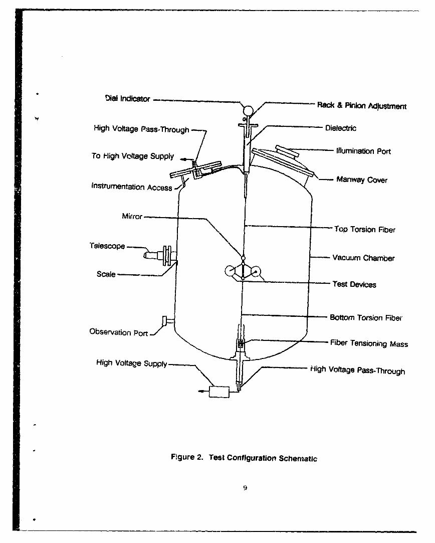
Dial indicator -- Rack & Pinion Adjustment

High Voltage Pass-Through Dielectric

To High Voltage Supply Illumination Port

Instrumentation Access -"a Cover

Mirror

Top Torsion Fiber

Tele,,L vacuum Chamber

Scale

Bottom Torsion Fiber

ObserationPortFiber Tensioning Mass

High Voltage Supply High Voltage Pass-Through

Figure 2. Test Configuration Schematic

9

1.17 m (46 in) straight side and a welded, dished top and bottom.

Access to the chamber was provided through a 0.51 m (20 in) top

manway. Smaller ports were also available and were used as

instrumentation and illumination ports. A 0.20 m (8 in) port

(not shown), offset from the chamber axis, was cut in the bottom

of the chamber. A surface flange was welded in place adjacent to

this port for close-up mounting of the diffusion pump. The

chamber was mounted on legs (not shown) with leveling screws for

adjustment of the vertical axis of the chamber.

Candidate propulsion test devices were mounted in tandem on

an improved, insulated figure-eight type device support. To

overcome the earlier problems encountered with the use of mercury

as frictionless electrical contacts, here a pair of tungsten

torsion fibers was used to feed high voltage electricity to the

test devices. One fiber was suspended from the top of the

chamber down to the test device support. A second fiber passed

from this support to a special mass--electrical contact

arrangement near the bottom of the chamber. The latter tensioned

the lower fiber and effectively produced a constant-tension, taut

torsion fiber system.

The electrical inputs to the test devices were fed from two

high voltage DC power supplies through low-loss, high voltage

pass-through fittings into the chamber. One pass-through was in

an off-center top port of the chamber; the other was in the

center bottom port. Cabling from the upper fitting connected to

the upper tungsten taut fiber through an electrically floating

(battery driven) electrometer. A similar electrical feed

arrangement was used for the lower tungsten fiber.

The conducting fibers, in turn, supplied high voltage to the

test devices via conducting arms of the device support structure.

10

A force measurement consisted of determining the average

angular twist of the taut torsion fiber system caused by action

of the force. This, together with the fiber calibration constant

and moment arms of the test devices, permitted the force on the

devices to be evaluated. The average angular twist of the

torsion fibers was measured using a telescope, mirrors mounted to

the test device support, and scales fastened to the chamber wall.

Torsion Fiber Subsystem

The measurement of forces generated by electrostatically

driven test devices was carried out using a dual, taut torsion

fiber subsystem. The test devices together with their support

structure were suspended by the upper fiber, and this unit

operated as a torsion pendulum in a dynamic mode. Accordingly,

the devices and holder were free to undergo small angular

oscillations about the vertical fiber axis with respect to an

angular equilibrium position. The torque to twist the fibers was

provided by the device or boundary generated force components

directed perpendicular to both the fiber axis and to radial

moment arms. These arms are defined by the fiber axis and the

central lines of force through the test devices.

Two such test devices were directed in tandem and mounted on

the figure-eight support structure shown in Figure 3, at "equal"

radial distances from the fiber axis. This revised device

support structure incorporated features of better electrical

isolation of component parts, better symmetry to minimize

asymmetric forces which are not test device related, and reduced

use of dielectric components to just a single central element.

The single element shown was a fire-polished 5.0 mm glass rod,

coaxial with the fiber used to join the identical top and bottom

aluminum conductor tubes of the support arms. The average moment

arm distances for tests conductec¢ in this program were 0.09778 m.

11

A

Insulating Glass Rod •Ball & Disk Test Device

Conducting Fiber Aluminum Arm

Figure 3. Tst Device Support Structure

12

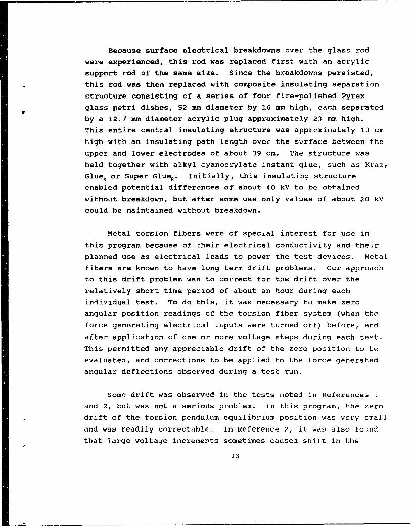
Because surface electrical breakdowns over the glass rod

were experienced, this rod was replaced first with an acrylic

support rod of the same size. Since the breakdowns persisted,

this rod was then replaced with composite insulating separation

structure consisting of a series of four fire-polished Pyrex

glass petri dishes, 52 mm diameter by 16 mm high, each separated

by a 12.7 mm diameter acrylic plug approximately 23 mm high.

This entire central insulating structure was approxi.ately 13 cm

high with an insulating path length over the surface between the

upper and lower electrodes of about 39 cm. The structure was

held together with alkyl cyanocrylate instant glue, such as Krazy

GlueR or Super Glue.. Initially, this insulating structure

enabled potential differences of about 40 kV to be obtained

without breakdown, but after some use only values of about 20 kV

could be maintained without breakdown.

Metal torsion fibers were of special interest for use in

this program because of their electrical conductivity and their

planned use as electrical leads to power the test devices. Metal

fibers are known to have long term drift problems. Our approach

to this drift problem was to correct for the drift over the

relatively short time period of about an hour during each

individual test. To do this, it was necessary to make zero

angular position readings cf the torsion fiber system (when the

force generating electrical inputs were turned off) before, and

after application of one or more voltage steps during each test.

This permitted any appreciable drift of the zero position to be

evaluated, and corrections to be applied to the force generated

angular deflections observed during a test run.

Some drift was observed in the tests noted in References 1

and 2, but was not a serious pioblem. In this program, the zero

drift of the torsion pendulum equilibrium position was vcry small

and was readily correctable. In Reference 2, it was also found

that large voltage increments sometimes caused shift in the

13

equilibrium position of the torsion pendulum, rut small

increments up to about 500 V left the zero position unaffected.

These observations were interpreted as a problem with the rise

rate (or ramp) of the voltage increment, rather than with the

magnitude of the increment itself. A variety of magnitudes of

voltage steps and rates of voltage rise to achieve these steps

were explored experimentally. It was found that voltage ramps up

to about 500 V/sec caused no appreciable drift or shift problems,

and this rate was used subsequently in most tests. The maximum

voltage rise rate for the driving power supplies was set at

12 kV/sec.

The torsion fiber chosen for use in this program was a

99.9C% pure tungsten fiber, 0.1 mm (0.004 in) in diameter.

Selected mechanical properties of tungsten fibers are given in

Table 113114.. Typically, the fiber strength becomes the limiting

mechanical factor for each candidate fiber material and

determines the corresponding minimum fiber diameter. Tungsten is

one of the strongest metal fibers, and the tungsten fiber chosen

is estimated to support a static load of about 0.57 kg. The

upper fiber length was 0.4282 m (16.86 in), and the lower one was

0.4001 m (15.75 in).

In implementing the dual torsion fiber system the upper end

of the top fiber was fastened to a vacuum sealed adjustable rod,

which could be raised, lowered, or rotated manually from outside

the chamber to achieve a suitable device height or angular

equilibrium position for tests.

The height adjustment feature for the fiber support rod

involved mounting the rod on a precision rack and pinion slide

mechanism. In use, this unit was coupled with a dial indicator,

and height settings and resettings to a precision of + 0.0013 cm

(± 0.0005 in) were achievable. An azimuthal angular scale was

fastened to the chamber, concentric with the movable fiber

14

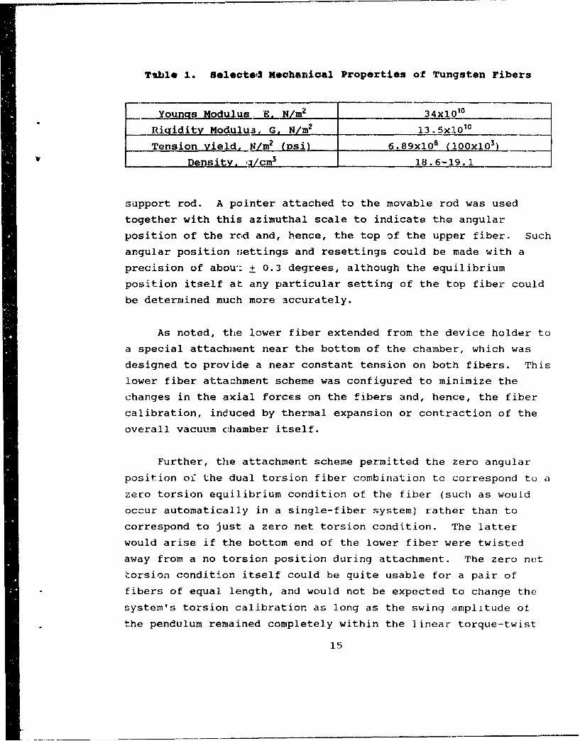
Table 1. Oelecto, Meohanical Properties of Tungsten Fibers

Youngs Modulus,, E. N/rn2 34x1010

"Rigidity Modulus5, G, N/mn2 13.5xLO0I

Tension yield, NLm 2 (Vsi) 6.89xi08 (100x10 3)V Density. .4/cm3 18.6-19.1

support rod. A pointer attached to the movable rod was used

together with this azimuthal scale to indicate the angular

position of the rod and, hence, the top of the upper fiber. Such

angular position settings and resettings could be made with a

precision of abou': + 0.3 degrees, although the equilibrium

position itself at any particular setting of the top fiber could

be determined much more accurately.

As noted, the lower fiber extended from the device holder to

a special attachment near the bottom of the chamber, which was

designed to provide a near constant tension on both fibers. This

lower fiber attachment scheme was configured to minimize the

changes in the axial forces on the fibers and, hence, the fiber

calibration, induced by thermal expansion or contraction of the

overall vacuum c:hamber itself.

Further, the attachment scheme permitted the zero angular

position of the dual torsion fiber combination to correspond to a

zero torsion equilibrium condition of the fiber (such as would

occur automatically in a single-fiber system) rather than to

correspond to just a zero net torsion condition. The latter

would arise if the bottom end of the lower fiber were twisted

away from a no torsion position during attachment. The zero net

torsion condition itself could be quite usable for a pair of

fibers of equal length, and would not be expected to change the

system's torsion calibration as long as the swing amplitude of

the pendulum remained completely within the linear torque-twist

15

region of the fibers. This feature will become clear by noting

that a fiber pair attached with an initial twist, would upon

awinging in one direction cause a further twist to develop in one

fiber of the pair and a relaxation of twist to occur in the

other. For fibers of equal length, the resulting torques would

still sum to the same total. Inasmuch as it was not convenient

to use equal length fibers within our vacuum chamber, and the

bounds Gf the linear torque-twist region were not well

established, we preferred to use the zero torsion equilibrium

conditions of the fiber, rather than the zero net torsion

conditions, in the experimental work under this program.

The special fiber tensioning attachment fastened to the

lower fiber near the bottom of the chamber is shown schematically

in Figure 4. This unit consisted of a inner pis'Con-like

cylindrical mass, which was secured to the lower fiber and was

free to slide axially between upper and lower stops within an

outer cylinder-like mass element. The inner mass was also

restrained by a pin in a vertical slot so this mass was not

generally free to slide angularly within the outer cylinder about

the fiber axis. The pin clearance of + 0.0025 cm (± 0.001 in) in

the slot, at the inner mass radius of 0.625 cm (0.25 in), could

have theoretically allowed the angular position of this mass to

be uncertain by + 0.23 degrees. In practice, the friction

between the two masses was adequate to prevent the inner mass

from moving during oscillations of the pendulum.

To ensure positive electrical contact between the two

conducting mass elements, a very fine, loosely coiled copper wire

was attached between the bottom of the piston-like component and

the lower end of the surrounding cylinder. Electrical connection

of the cylinder element with the conducting platform on which the

cylinder rested when in place for a test, was by direct.

mechanical contact.

16

Torsion Fiber

Movable Mass

Alignment Pin

S. . ..O uter M ass

Figure 4. Fiber Tensioning Device

17

This fiber tensioning unit was used in conjunction with the

height adjustment feature to set, and reset, the azimuth of the

zero equilibrium position of the torsion fiber pendulum with

respect to the chamber. The fiber was raised, without breaking

the vacuum seal, until the lower composite mass was totally free

from its bottom support. The top fiber was then rotated a known

amount by turning the height adjustment rod in relation to the

azimuthal scale of the top of the chamber. The pendulum

oscillations induced by this action were then allowed to totally

subside.* The fiber was then lowered so the composite mass

again rested on the lower support platform. The inner mass was

then raised about 2.5 mm (0.10 in) without lifting the outer

element of the composite mass from the platform, so the inner

mass element was suspended by the lower fiber. Thus, the weight

of the inner mass again caused tensions in the upper and lower

fibers to return to essentially their original values before the

repositioning.

Optical Readout and Data Acquisition Subsystems

A readout subsystem consisting of a simple telescope, two

mirrors and two scales was used to determine the average angular

deflection of the pendulum and, hence, the corresponding twist of

the dual torsion fiber system during tests. An alignment

telescope equipped with a cross hair reticle was directed to

view, via reflection from one of two mirrors oriented near right

angles to each other, one or another of two linear scales mounted

on the inside wall of the chamber. A definite reading could then

Such pendulum oscillations damped very slowly under high

vacuum conditions, sometimes requiring two to three days. Later inthe program it was found that the overall time could be shortenedvery simply by increasing the chamber pressure to about 10 3 torr,letting the Fendulum come to rest, and then pumping the vacuum backto about 10' torr. This cycle time typically required less thanone day. In retrospect, it is recognized that more direct dampingtechniques could have been used.

18

be determined at the intersection of the cross hair with thescale image. Because the optical path used included a reflection

from a mirror, the apparent deflection read through the telescope

directly from either scale on the chamber wall corresponded to

exactly twice the angular rotation of the pendulum,

Each linear scale consisted of three stainless steel,

flexible machinist's scales 0.6096 m (24 in) long withsubdivisions in English units of 1/50 in. These machinist's

scales were carefully welded together at the ends to make eachlinear scale continuous. One such complete scale was mounted

just above the telescope viewing port and was viewed using one

mirror. The second complete scale was mounted below thetelescope viewing port and was seen using the second mirror,

oriented near 90 degrees in azimuth ckbout the fiber axis from the

first mirror. The scales were sufficiently long to permit both

to be seen simultaneously using one of the mirrors. Thispermitted the scales to be compared, and readings taken on one

scale to be consistently converted to that of the other. Thus

only one set of final scale readings were employed.

In this arrangement the radial distance, r, from each mirror

to its corresponding scale was 0.5175 m (20.38 in).

For convenience in testing, the extremes of the apparentangular deflection (expressed as scale readings), rather than

continuous or other periodic values during complete oscillations

of the pendulum, were recorded as data. By averaging the

extremes, the positions of the centers of oscillation weredetermined both when an applied torque was present and when itwas absent. The differences between these averages gave the

deflection of the pendulum associated with the appijed torque.

Each scale was typically read to the nearest 1.27x104 m(0.005 in), and the central position ou each individual

19

oscillation measure was determined to the v.ame degree of

uncertainty. A typical force measurement during a test involved

about ten oscillations, so the calculated uncertainty of the mean

was about 0.40x10"4 m (0.0016 in). However, taking into account

reading uncertainties and system noise, a somewhat larger

deflection of about O.b4Xl0"4 m (0.0025 in) is helieved to be

representative of the threshold of measurements. This results in

a minimum deflection angle of the mirror

Omn =' 6.14x10"5 radian per 0.0025 in

apparent motion of the scale.

This value of Omin corresponds to about 13 seconds of arc, which

is not of great sensitivity, but is about four times better than

was achieved under the Phase I program.

During the initial set-up of the propulsion device tests

some observations were made visually through the telescope. The

preferred technique employed in essentially all routine test runs

involved ising a video camera and monitor, with the camera lens

positioned to see through the telescope eyepiece. Deflection

readings during tests were then made directly from the video

monitor. These were entered manually into a computer, after

first pressing a single key to record the time (supplied by the

computer) to which each reading corresponded.

A General Electric VHS movie Video System SE9-9108 .,ith

video tape recorder was used for most of the test runs. Use of

the recorder permitted a real time record of the actual test run

to be made. This record was helpful since it permitted replaying

the test run to confirm deflection readings or to ascertain

missed readings after-the-facc.

Readout of the per,(Tilum oscillations for torsion fiber

calibration--carried ouc by measuring the swing periods of the

20

fiber as part of a torsion pendulum--required a different

approach from the video camera technique used during force

measurement tests. This is because the swing time periods cannot

be determined visually with sufficient accuracy. In this case, a

pendulum bob of known mass, geometry, and moment of inertia was

used with the fiber to be calibrated, in place of the actual test

devices and their support structure. The same telescope and

mirror system was again used, but an active signal in the form of

a laser beam was passed through a beam splitter, through the

telescope, and onto the mirror. Twice each period as the mirror

oscillated, the laser beam was reflected back through the

telescope, into the beam splitter and deflected into a fiber

optic cable and then onto a photo detector and amplifier. Real

time electrical signals from the detector amplifier were sent to

a digital oscilloscope and recorder, where the signal pulses were

displayed and timed accurately.

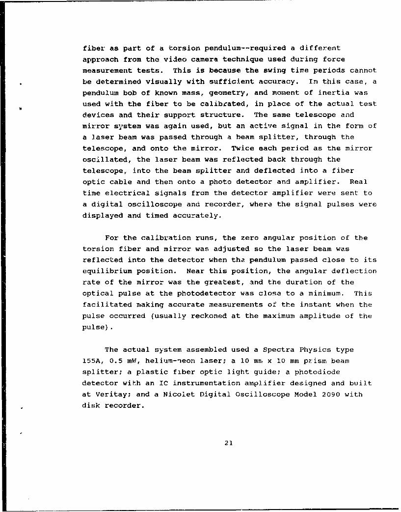
For the calibration runs, the zero angular position of the

torsion fiber and mirror was adjusted so the laser beam was

reflected into the detector when the pendulum passed close to its

equilibrium position. Near this position, the angular deflection

rate of the mirror was the greatest, and the duration of the

optical pulse at the photodetector was close to a minimum. This

facilitated making accurate measurements of the instant when the

pulse occurred (usually reckoned at the maximum amplitude of the

pulse).

The actual system assembled used a Spectra Physics type

155A, 0.5 mW, helium-neon laser; a 10 mm x 10 mm prism beam

splitter; a plastic fiber optic light guide; a photodiode

detector with an IC instrumentation amplifier designed and built

at Veritay; and a Nicolet Digital Oscilloscope Model 2090 with

disk recorder.

21

Typical digital sampling times used were 0.35 sec per point.

At this sampling rate, a total sample of 32x10 3 points (26.7 mini)

could be recorded directly. The total time used for calibration

runs encompassed about eight to fifteen complete oscillation

periods.

Electrical Subsystem

"The high voltage sources to drive the devices under test

consisted of a pair of Spellman regulated, 0-60 kV, DC power

supplies, Model UHR60PN30, each of which hLd a maximum power

output of 30 watts. The voltage polarity of each supply was

reversible internally, but was not directly swi.tchable for safety

reasons. These two separate high voltage power supplies could be

grounded at a common earth ground and operated "back-to-back,"

with one providing a negative voltage and the other a positive

voltage. This enabled one electrode of each test device to be

set at an arbitrary positive potential with respect to ground,

and the other electrode to be set at a selected negative

potential. This also allowed complete flexibility in setting the

potentials of the device electrodes relative to the grounded

chamber.

The high voltage was fed from the supplies to the test

chamber and devices using high voltage cables, each rated with a

DC brerkdown voltage of 100 kV. Lesker VZEFT-10, 50 kV

electrical feed throughs, configured for vacuum operation, were

used to bring the high volt.oge Into the vacuum chamber.

In this program, we chose to operate and control the high

voltage supplies, together with two electrometers used for the

measurement of combined current through the two test devices,

with an IBM XT cormiputer. Several advantages were associated with

this choice, but the main ones were: (1) to permit software

changes rather than hardware modifications in this part of the

22

system as certain test requirements and procedures varied; and

(2) to enable the high voltage power to be applied to the test

devices in a repeatable fashion from test to test without manual

manipulation.

In addition, the computer used for this control also

functioned as a data logger. Data from both the power supplies

and the electrometers, along with information entered from the

keyboard, were automatica]lly stored in a random file during each

test. Hardcopy results in tabular or graphical format from this

file were readily produced subsequent to each test run.

The programmed variables for the high voltage supplies

included voltage output levels, and time rates of voltage change

(rise and fall) for reaching these levels.

To implement this approach both power supplies were first.

modified internally for remote operation. The XT computer was

then outfitted with two peripheral boards to provide the

necessary I/O capabilities for controlling the two systems. One

I/O device was used to handle voltage program levels and

monitoring of both high voltage supplies; a second I/O device,

specifically designed by Veritay, was used to handle 16 bit

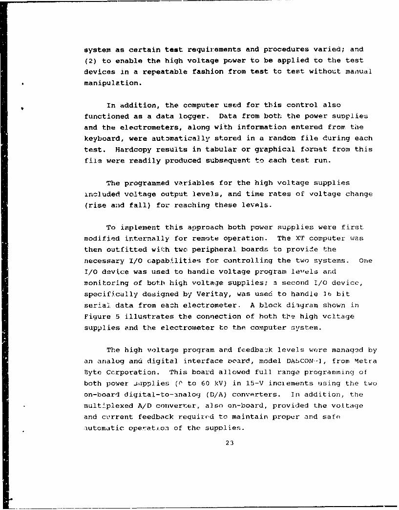
serial data from each electrometer. A block diagram shown in

Figure 5 illustrates the connection of both the high voltage

supplies and the electrometer to the computer system.

The high voltage program and feedbaik levels were managed by

an analog and digital interface ooard, model DASCON1-, from Metra

Byte Ccrporation. This board allowed full range programming of

both power ja~pplies (P to 60 kV) in 15-V inclements using the two

on-board digital-to-3nalog (D/A) converters. In addition, the

multiplexed A/D converter, also on-board, provided the voltage

and cvrrent feedback requir,•d to maintain proper and safe

automatic operati.on of the supplies.

23

rWNC "r MACKI

SFigure 5. Block Diagram of High Voltage Control and Current Data Acquisition

A complete test could be preset into the computer using the

associated control and data logging software. Program flow

evolved around several loops and interlocks to ensure that data

acquisition was continuous for inputs from both the keyboard and

the I!O board, while the power supply settings were changed

automatically or by manual activation. Safeguards and various

visual annunciators incorporated in the program apprised the test

operator of problems, s~uch as high voltage breakdown or lost.

communication with I/O devices. The system also had the

capability of complete shutdown in the case of failure of a key

component.

24

The instrumentation to measure low level electrical currentthrough the test devices was specifically configured toaccommodate the high voltage of interest, to minimize losses, andto operate inside the vacuum chamber as close as possible to thetest devices. A two-current sensor system was used, one to sensethe current in the upper conducting torsion fiber, and the otherin the lower fiber. Each such sensor unit had a set ofcomponents inside the chamber and another set outside. Eachinside sensor set was designed as a miniaturized, self-containedbattery powered unit which could operate electrically isolated atthe level of the high voltage input to the test devices. Theinside set consisted of an electrometer with an A/D converter, anelectrically isolated battery power supply, and an electro-optictransceiver. The outside set consisted of another electro-optictransceiver, an I/O interface board, and the same IBM XT computerused with the high voltage power supplies.

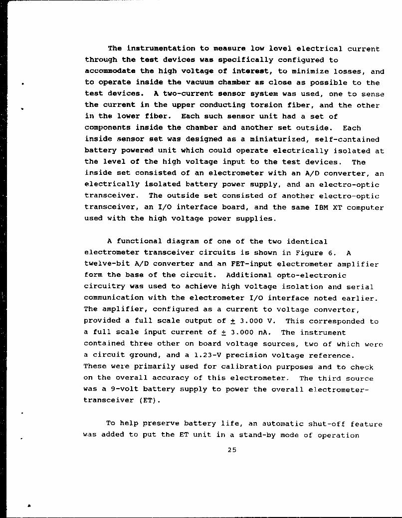
A functional diagram of one of the two identicalelectrometer transceiver circuits is shown in Figure 6. Atwelve-bit A/D converter and an FET-input electrometer amplifierform the base of the circuit. Additional opto-electroniccircuitry was used to achieve high voltage isolation and serialcommunication with the electrometer I/O interface noted earlier.

The amplifier, configured as a current to voltage converter,provided a full scale output of + 3.000 V. This corresponded toa full scale input current of + 3.000 nA. The instrumentcontained three other on board voltage sources, two of which werea circuit ground, and a 1.23-V precision voltage reference.

These were primarily used for calibration purposes and to checkon the overall accuracy of this electrometer. The third sourcewas a 9-volt battery supply to power the overall electrometer-

transceiver (ET).

To help preserve battery life, an automatic shut-off featurewas added to put the ET unit in a stand-by mode of operation

25

!4

Figures6. Functionall Dliagram of Electrometer-Transceiver

while it was not in use (i.e., when it was off line with the

couputer system). This disabled all but the photodiode receiver

circuitry. This was a necessary feature as frequent battery

replacenents were not feasible around the sensitive torsion

fiber--- where the ET unit was located. The ET unit on stand-b'

could be reactivated by a "wake-up" signal generated by the

(outside) I/O interface and sent as an optical signal from theoutside transceiver to the inside one. In the standby mode, the

circuit exhibited minimal draw on the power source--apprzximateiy

1/50 of the maximum quiescent current drain of the entire unit--

and thus extended battery life.

The accuracy of each electromfeter unit was assessed by

observing/calibrating the electrometer input/output

26

pM 1

characteristics prior to installation in the vacuum chamber.

This action was performed using known current level inputs and

comparing the output using a Fluke digital voltmeter. Error

correction factors were determined and compensation was applied,

using computer software, thereby eliminating the need for

additional circuitry. The overall accuracy obtained was

estimated to be within 0.1 percent.

Each electrometer transceiver unit was installed in a

stainless steel enclosure, as shown in Figure 7. One such

enclosure is located at the upper end of the top torsion fiber;

the other near the lower end of the bottom fiber. The

electrometer was fabricated on a flexible printed circuit board,

which was situated with its major electronic components against

the inside wall of the steel shell. This provided additional

shielding as well as a heat sink for the A/D converter and for

the electrometer amplifier---a relevant consideration in a vacuum

environment. A sealed acrylic case housed the 9-volt lithium

battery used as the main power source; this plastic case also

served to contain any cell leakage that might have occurred,

thereby minimizing the risk of vacuum chamber contamination.

Electrical connections between the circuit board and the test

device were made using a double-sided conductive plate. The

plate itself was easily slipped into spring loaded contacts at

the upper and low termination locations of the torsion fibers.

The optical link between inside and outside ET units was made

through plastic optical fibers. This use of optical isolation

helped overcome severe problems of electrical insulation, losses

and chamber wall pass-through that would otherwise have been

associated with direct electrical wiring.

Vacuum Subsystem

The vacuum system used for tests is shown schematically in

Figure 8. It consisted of a CVC Model PAS-66D expanded 6-inch

27

Pd"J TNRKALSSMAED 9 VOLTNATTKRY CASE

Rffwsm

Opr"/

"MR/

Figure 7. Electrometer-Transceiver Configuration

28

CD.

E

00(U d0L 0

8>

0.

-E

uU

> >

E .50

UU

E E9

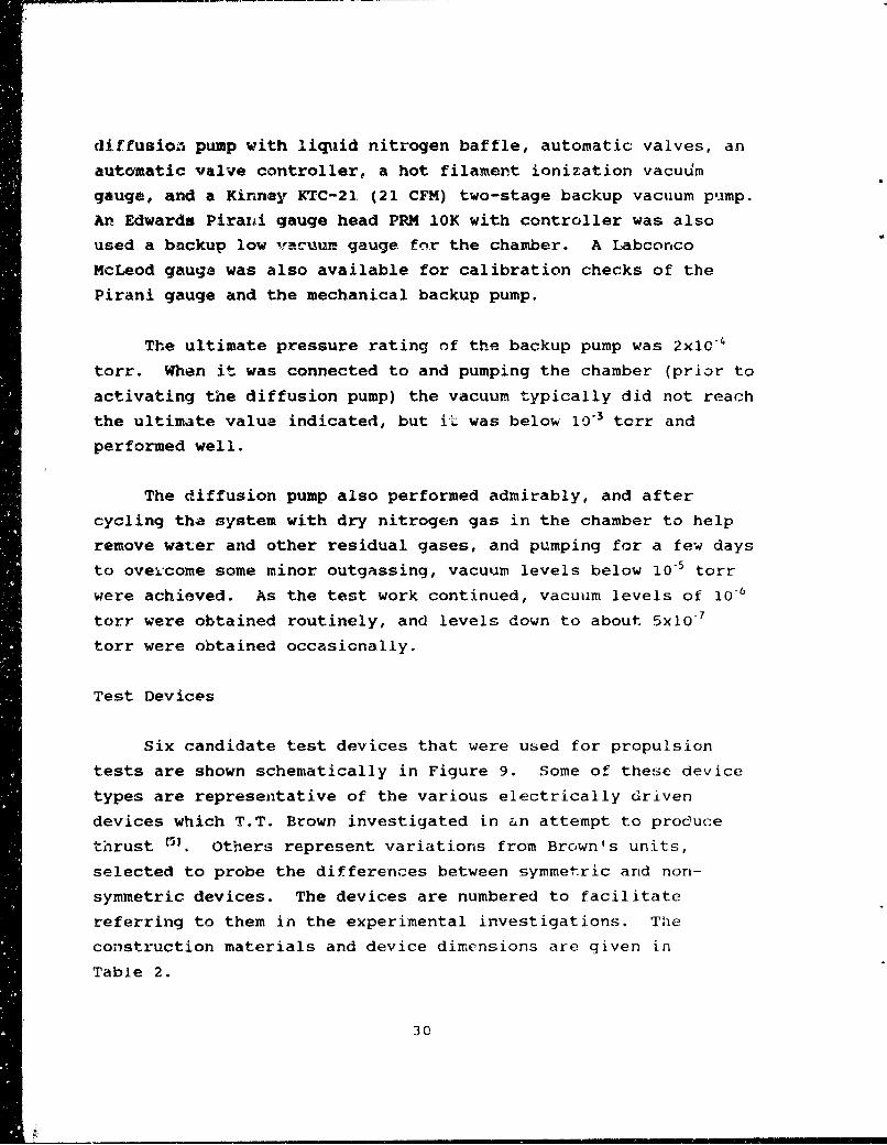
diffusioa pump with licpiid nitrogen baffle, automatic valves, an

automatic valve controller, a hot filament ionization vacuum

gauge, and a Kinney KTC-21. (21 CFM) two-stage backup vacuum plimp.

An Edwards Pirani gauge head PRM 10K with controller was also

used a backup low vacuum gauge fnr the chamber. A Labconco

McLeod gauge was also available for calibration checks of the

Pirani gauge and the mechanical backup pump.

The ultimate pressure rating of the backup pump was 2 X10-4

torr. When it was connected to and pumping the chamber (prior to

activating the diffusion pump) the vacuum typically did not reach

the ultimate value indicated, but ii- was below 10'3 torr and

performed well.

The diffusion pump also performed admirably, and after

cycling the system with dry nitrogen gas in the chamber to help

remove water and other residual gases, and pumping for a few days

to overcome some minor outgassing, vacuum levels below 10,5 torr

were achieved. As the test work continued, vacuum levels of 10-6

torr were obtained routinely, and levels down to about 5x10' 7

torr were obtained occasionally.

Test Devices

Six candidate test devices that were used for propulsion

tests are shown schematically in Figure 9. Some of these device

types are representative of the various electrically ariven

devices which T.T. Brown investigated in an attempt to produce

thrust t5l. Others represent variations from Brown's units,

selected to probe the differences between symmetric and non-

symmetric devices. The devices are numbered to facilitate

referring to them in the experimental investigations. The

construction materials and device dimensions are given in

Table 2.

30

Z

00 00 0

SIDE VIEW FRONT VIEW SIDE VIEW FRONT VIEWNo. I Ball and Plate No. 4 Symmetric Bali

Mac @ CM @

SIDE VIEW FRONT VIEW SIDE VIEW FRONT VIEW

No. 2 Ball and Plate With No. 5 Syrmnetric Ball With1/4-Inch Diameter Dielectric 1/4-Inch Diameter Dielectric

0

SIDE VIEW FRONT VIEW SIDE VIEW FRONT VIEW

No. 3 Bali and Plate With No. 6 Symmetric Plate1/2-inch Dielectric

Figure 9. Test Device Types

31

0

$40

0

00 i 0 01(1 n 00

$4 a .l k - O

as940 'm 0 N N

w 9~ 1. 1 9o 0 001 00 0 R c

0 g I 0 0o 0 0 0

'0 ffl

* 00

* 1. 0 0 101*~ 0 0 10--

A*- 0 ý4r - -4 r-0)1- -

164 000)0 0 0 0 0

o 1- Ngo

0 U) 0 PU

@1 ~ ~~~~ .z, (No wN Clý < x4'0 ' . 'O, ( N '

94~- -H N-4"I H N 0 0 H -4O14 0 0 0 &N O O O O O O O C

E44 14J NOo o oo OO N 40 u -

r ~ ~ -4 f i -A' - a-4H -H m (

_ _)0

a)32

It will be noted that Test Device Type No. 2 was configured

for different tests with two different types of dielectrics,

acrylic and lead titanate-lead zirconate.* The dielectric

constant of the former is about 3.5, and the latter is about

1750.

The basic ball and plate unit was a device type used

extensively by Brown, and apparently with some success in

generating propulsive forces. While the devices Brown used

normally included a dielectric, the devices tested here were

configured both with and without dielectrics. A key feature of

this test unit, according to BrownE51 is that it would develop a

nonlinear electric field between the ball and plate.

The symmetric ball, or symmetric plate, test devices were

expected to develop symmetric electzic fields between the

electrodes and, again according to Brown 5, should qenerate

mininal or zero propulsive forces.

TEST RESULTS

Test Approach

The overall test approach emphasized the direct measurement

of propulsive forces under high vacuum conditions. Direct force

measurements were considered essential since the nature and

characteristics of the forces under investigation were unknown.

From the space propulsion point of view, the very existence of

this propulsive force in a vacuum was of key interest. A known

phenomenon called electrical (or ion) wind has frequently been

"This is a piezoelectric cera-iic material designated Channel5500 by its manufacturer, Channel Industries, Inc., Chesterland, OH44026.

33

invoked as a mechanistic basis of thrust on electrostatic-driven

propulsion devices similar to, and including, those explored by

Brown. Electrical wind does, in fact, contribute to the thrust

on such test devices when they operate in air. In a vacuum,

another force contribution, known as ion propulsion, is known to

be operative, but is usually quite small unless very large

electrical currents or current pulses are used. This ion

propulsion results from a transfer of momentum to the body of a

test device (or an ion engine), as a result of the electrical

ejection and acceleration of ions unidirectionally from an

ablative source within the engine.

At the outset of this program a choice was made to drive thete.t devices using steady electrostatic potential differences

between the electrodes of the devices. Generally, it was also

understood, on the basis of Brown's comments (Reference 1, page 8

and Reference 5) that the thrust existed under high vacuum

conditions," Khen there was no vacuumn spark." (A vacuum spark--

or breakdown--might have been adequate to account for the thrust

just on the basis of the ion propulsion effect alone.) Near the

very end of this program, we briefly examined the force

generation effects with pulsed fields, under near breakdown

conditions. The overall test set-up for this program was

configured in accord with the primary choice to drive the test

devices with DC voltages. An alternate configuration would

likely be more appropriate for a non-DC voltage drive.

With this constraint, a principci concern and unknown for

the test effort was the influence that the tank wall boundaries

might have on the forces exhibited by the electrostatically

driven test devicer. Two means were employed to examine the

influence of tank wall boundaries. The first, and simplest

scheme, used two mirrors oriented at right angles to each other

and mounted on the test device support. This, together with the

scale mounted on the vacuum tank wall and the ability to reset

34

the zero equilibrium position of the torsion pendulum to any

azimuth, permitted force measurements to be made at various

equilibrium positions over a 180 degree range. This range was

commensurate with one full angular pericd of the two-device

support structure. The force measurements, in turn, made it

possible to detect any significant asymmetries in the total force

on the test devices.

The second scheme employed a 0.20 m (8.0 in) square"'boundary plate" fastened to a vacuum-sealed movable rod and

located inside the chamber. The rod and plate were electrically

grounded to the chamber wall and could be positioned from outside

the tank, so plate was at a given radial distance from the wall.

The objective of using such a plate was to determine whether the

plate introduced asymmetries in the force measurements as a

function of relative azimuthal position of the test devices and

plate. Also it was used to determine whether such boundary

effects would disappear as the plate approached the tank wall.

Calibration

Calibration of the dual torsion fiber system was carried out

by measuring the period of tthe torsion pendulum, consisting of

the fibers, a calibration nass (which was substituted for the

test devices and their support structure) and the mirror holder.

Results for the pair of fibers used throughout the tests are

given in Table 3. The torsional stiffness, S, of the tiber pair

operating as a system was calculated using the equation

35

_ T2 ,(1)T T2

where

Q - total torque; N-m

0 = angle of twist of the calibration mass and mirror and,

hence, of each fiber; rad

I = moment of inertia of the suspended mass; kg-mr2

T = oscillation period; s.

An analysis of a damped oscillating torsion pendulum'?' has

indicated that the true value for the torsional stiffness, S,

given by equation (1) requires the use of the period T. of

oscillation of the undamped pendulum. However, it is known that

the dual fiber system used here operated as a damped oscillating

torsion pendulum, and it war' assumed to be driven by a time-

inuependent force pulse, which acted over several oscillation

periods. The damped oscillations of this type of system are

mathematically riot periodic functions, but they do exhibit a

consistent conditional period, T,. It is this conditional period

T1, which is measured to determine S. It is necessa'-y to examine

the relationship between these two periods in order to determine

an accurate vala.e f...r S.

The oscillation of such a damped pendulum can be

char'ýcterizd for the present application by only two

quantities:***

In general, two more quantities are required: theconditional amplitude, K, for a given time, and the phase angle acf the various components which comprise and characterize Lh•oscillations (see Pele:ence 6).

36

(no 0 . ,

oLn 00 0H

UN0 00

f- 0

Ln r-4 '0%

IC e4 .4O m 0 0

COx x

('4 * 00

0n 0,O

* Ir. Ch

fn x Nr

o 00

0- a -

X- LA o7 0- -es LO m

Ca~~ ~~ (1 H a 'X H0 0 N1Ofn. *N .,o 0 >o

44 .4 *'U) LA -. ,0 H H0 f4r4f4co co 0; r-4 N9:N - 00

00 00 0 ý*64 ov0-1 0 0 0

Id0000 1- 0 N Ch4

4)x X x %D x x '41 H to 00 0 .0 t L

w 0- NHit'v v ) 00 . 0 * ~tW0NHýDo Lo CO .u 00 00

c) - -co H N w

0q 0 xE-4 00 f-4

G- No -W 1

* . o W, _ _ _ _ _ - ta, ~ - - X_ _ _ -. - - C) >NN

oI t

04 Q)4) 4

0 0 44 204 'H C) 0. O

V I~ 0, n. In0 00C)4 0 0~ 41 ..4 u .,4-4 M 1 -

E-4aM.JU H HS 4) (0 En 0 )

a) ý4(1 VJf~ c 4JO MU -4 wI U3 .4 1 t: t) (n 4-4 UrQ rQ~ 4J M 14 4-' a, 0 ) 0-') 04-) 0 H

37

T,, the conditional period of oscillation, which represents the

time between consecutive zero amplitude crossings in the

same direction (this also corresponds to the conditional

angular frequency wO)

d, the logarithmic decrement, a dimensionless measure of the

damping, which is the natural logarithm of the ratio of

angular displacements one period apart. It is related to

the conditional period, T,, and the damping coefficient h,

and the pendulum swing amplitudes O(t) by

T(t) (2)d=Th= n ( (t+T )•

From the reiation[61

~2 _ h 2

where h is the damping coefficient, and w0 and w, are the

respective angular frequencies for the undamped and damped

oscillations, S can be expressed as

STI I 1+ h (3)

These angular frequencies, in turn, are related to the

oscillation periods by

38

•-27t (4)° To

and

2n (5)Ti

The measured value of h for the dual torsion system with

tungsten fibers was about 5.0 x 10,5 s-1. The ratio (h/l 1) 2 , which

was approximately 2.2 x 10-7 for the devices tested and smaller

for the calibration mass used, was, therefore, negligible in

Equation (3). In turn, S was adequately approximated using

Equation (I) with T = Ti z To.

From the Phase I work, it was learned that the effect of

temperature on the fiber calibration values was apt to be

significant. The variation in torsional stiffness, S, of the

dual tungsten fiber system with temperature is shown in

Figure 10. The points indicated in this figure correspond to the

data from Table 3, except the values at the two highest pressures

for test numbers 4c and 5c were not used. As a result, the

calibration curve in Figure 10 corresponds to vacuum levels over

the approximate range of 13.3 Pa (lxlO"1 torr) to 1.33x10- Pa

(1x10" 6 torr). At 20°C (68°F) the temperature coefficient

measured for the torsional stiffness is -0.033 percent per degree

Celsius increase (-0.019 % /°F).

The rigidity modulus, G, for the fibers in each pair were

assumed to exhibit the same value, since this modulus is

characteristic of the fiber material and geometry, and since the

fibers were cut from a single longer length of material.

39

TEMPERATURE - K

&,370 1

0

6.360

E

z 6.3mU.

U.

04

-6.3 •0IL.3355w 5M 5808

04

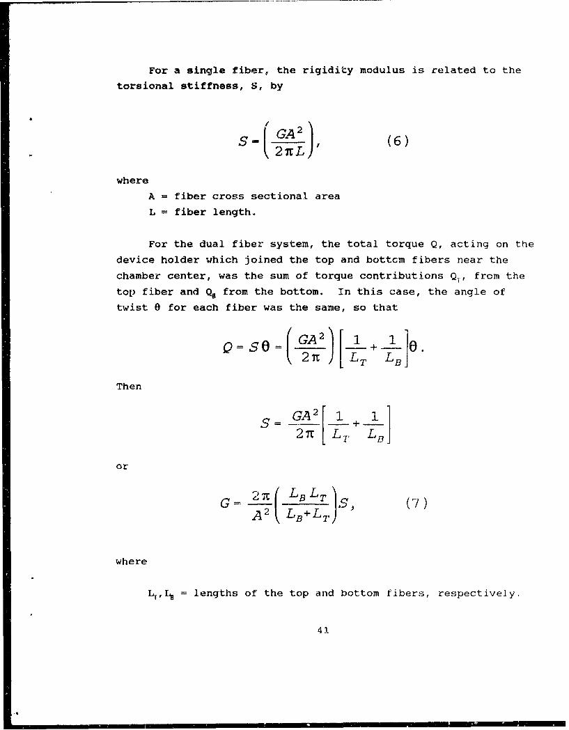
For a single fiber, the rigidity modulus is related to the

torsional stiffness, S, by

SI 2iuL)' (6)

where

A = fiber cross sectional area

L = fiber length.

For the dual fiber system, the total torque Q, acting on the

device holder which joined the top and bottcm fibers near the

chamber center, was the sum of torque contributions Q,., from the

top fiber and Q. from the bottom. In this case, the angle of

twist 0 for each fiber was the same, so that

Then

or GA2 1 +4 1 ]2n LT L (

or

A 2 (LB+LT)

where

L T, I= lengths of the top and bottom fibers, respectively.

41

The rigidity modulus was calculated using Equation (7),

together with the temperature dependence of S indicated in

Table 5 and Figure 10, to obtain the value G = 13.38x1010 N/m 2 at

20"C. The exact temperature at which the handbook value€3) of

GH = 13.5x10I 0 N/M2 was determined is not known, but room

temperature (often taken as 20"C) is likely. As can be seen, the

value calculated here compares favorably (within about 0.9%) with

the handbook value.

The test device support unit with two mounted devices of

type No. 1A was run as a torsion pendulum in order to determine

the moment of inertia, Is, of this system. Equation (1) was

solved for Is, using the known value of S for the fiber pair and

the approximation T=T,. Separate determinations of Is for device

1A gave the values shown in Table 4. It will be noted that there

is a significant change in the swing period and, hence, the

calculated values of Is with vacuum level. The value of

Is = 4.4868 x 10i 7 kg-m 2 obtained for Test No. 10C at a vacuum

level of 1.33 x j0-3 Pa (1 x 105 torr) is likely the best value,

but without replication and further investigation it remains

suspect.

In principle, this value (or an improved one) could have

been used with this particular torsion pendulum to check or

recalibrate the torsion fiber pair directly, without the need to

reuse the calibration mass. This recalibration approach was not

actually used, in part because of the above noted sensitivity of

calculated Is to the vacuum level, and in part because a number

of different test devices were used and a relatively large number

of tests would be required just to obtain the individual moments

of inertia for each case. Rather, the calibration mass, itself,

was reintroduced after the data runs began, to obtain another

calibration point at a higher temperature, as indicated in

42

oa I 0 a 0

-H 0'

IN ~ to 00 c

0'.A0

.A L

co4 - 1 - f 4 -4 1 o im -

X I0 W-4

-.4 0 0

H c44 cc O 4 X 0- H

H InN L N H 0 0% 0W 0'o

a a a 000c

$4- -4-'

t7o o o InIu c ' x 0 (N 0'

I-4 0 10 H In '~ .,

E-4 0 0r vAI r-AE4

-- J~J' M 4 "I Il -4 W

coOO co( 0 0 o

(a ý4 X 4)0u 4 t 0004(n0)Z' IHJ 1 - -4H

4J~-c0 L 0 '-P -A 44 Ha)

(1 41N w .- 4 41 +1' +1 (n (4LA

ul >

43J

Figure 10. This recalibration test also helped confirm that this

value was consistent with earlier values--even though a

temperature change was involved.

It should be noted that only the moment of inertia I. of the

support with the devices needs to be known in order to

recalibrate the fibers with the test device pendulum. The

original fiber calibration value of S can be used to determine

the force generated by eny particular device pair, provided the

temperature is taken into account, and the axial tension does not

alter the value of S. The fact that a moment of inertia 1. was

not determined for each of the device types did not precludedetermining force values from deflections observed during tests

with each such unit.

The force, F, on each test device was obtained directlyuning the expressions:

(X (X- ) /)/2r, (8)

OQ-S ,and (9)

F- Q/2R, (10)

where

-Xo= zero equilibrium position of pendulum on a linear scale

x - final equilibrium p4,sition of pendulum on a linear

scale

r = mirror to scale distance = 0.5175 m (20.375 in)0 = angular deflection of mirror and devices, and angle of

twist of the torsion fiber; rad

S = torsional stiffness (at a given temperature); N-m

Q = total torque on fiber; N-m

44

R = moment arm of each device about fiber axis; 0.09785 m

(average)

F = force on each device; N.

These relations were combined into the following single

expression for evaluating F:

F- kAx, (1i)

where

k_ (12)4-rR'

Ax = (x-x 0 ) , (13)

and k becomes temperature dependent. This expression for F was

used in reducing test data under this program.

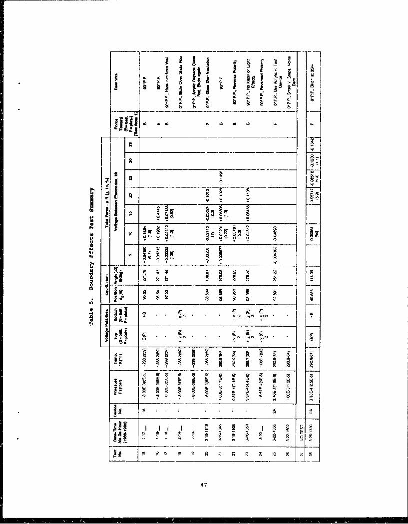
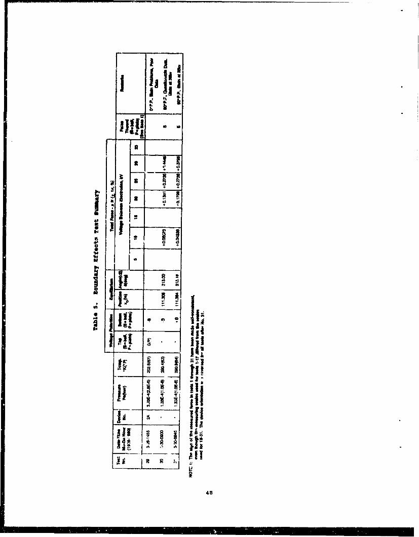
Boundary Effects

Initially it was suspected that force measurements made with

the torsion pendulum arrangement might be influenced by induced

surface charges on the walls of the vacuum chamber surrounding

the test devices. Since reasonable care was taken to ensure

construf-tional symmetry in the pendulum, the device support

structure, and the test devices, all with respect to the chamber

axis, the main boundary effects--if any--were expected to arise

froxa features which might upset this symmetry. This could

include various ports JIn the chamber, the shielded cables, small

protuberances on the chamber wall, etc.

Force measurement tests to check various featu)res of the

system and to explore the nature of the boundary effects are

summarized in Table 5. The initial six tests were for tne

45

Pm

I I

9- d+ + +

+, ++ +,q, 9: 9 + + q;,, !.. | ! + a., ,A+ +

t.,,

* ++ a. ++ *• b+ + 2.

JJ T . A. A A 0 U m A..' . ,,7 ,,.

C4~ R

,-+ ~ ~ c f. . : ,. .: ,,: (6 co + '

4i < . . .

46

j & ~ 6 ~'G0. 0 j ~I ICA:

0I

to : w . IL m C

- C. .. b . * aý ul

0 0 _ _ __a,~f~1 w . 02 02 +

+ .+ +r

IE I

-IL +

a6 iq Zf Zl Zý" iq Z

U) uJ Wj wU8. 8 82 u w .# .*

c6 .. 06 'W W~~ W JC 0 2

.6 4 If

47

I--A'

j Ji

-+ • LAI- _

HiII

448

shakedown of the new torsion pendulum system and toe power

supplies. Drift of the equilibrium position of the pendulum was

found to be non-zero, but was generally steady and rather small,

and was, therefore, readily correctable. In Test No. 2, for

example, the zero drift was significant, was about 0.00114 in pe'r

swing of the pendulum, and was consistent over 50 swings (about

22 min) during the test run. For these tests, the measured

forces were small, and varied approximately as the second power

of the driving voltage between electrodes of the test devices.

Test No. 7 was conducted using a zero equilibrium position

shifted by about 90 degrees with respect to that used for the

first six tests. The indicated angular position 0 corresponded

to the observed position x0 on the tank mourited scale, as seen it

the second mirror (shifted by about 900 with respe.,t to the first

mirror). The exact values of the position x0 and angle 6 shown

in Table 5, were determined from corrections obtained by reading

a single scale using both mirrors, and by reading tw.o scales

using a single mirror.

In Tests 8 through 10, successive amounts of aluminum foil

shielding were added over various chamber ports and feed

throughs. Test No. 9 results should be disregarded as a computer

shutdown of power was experienced, together with a large zero

shift in pendulum equilibrium position.

Test Nos. 7 through 10 gave the first indications that some

type of boundary effects were significant, in that the direction

of the forces for these tests (with a 90° shift in zero

equilibrium position) was reversed from the direction obtained

when the equilibrium position of the pendulum was near zero

degrees.

To confirm that this was the case, and the shift in force

direction was not due to effects arising from application of the

49

aluminum foil shielding, or from some residual ion generation

from the ion vacuum gauge, Test Nos. 11, 12, and 13 were run.

These tests confirmed the reversal in direction of the apparent

force with change in pendulum equilibrium position. The

corresponding forces for these tests were in better agreement

with each other, even though their magnitude was not the same as

observed in Test Nos. 7 through 10.

In further search of possible boundary effecta, Test Nos. 14

through 16 were run, aqain near the 90" pendulum position, but

with the top fiber grounded, so the electrical potential to the

test device was applied through the bottom fiber. This choice

was in response to the belief that some residual boundary effect

was arising from the inability tq properly shield the off-center

electrical feedthrough at the top of the chamber. With the top

fiber grounded, such an effect should have disappeared; but it

did not.

Test No. 17 was conducted in the same 900 pendulum position,

with the grounded boundary plate moved inward 2.5 cm (1.0 in)

from the tank wall toward the pendulum. The corresponding

variation of the apparent force with applied voltage, V, changed

from approximately a V2 dependence to one of about V2.7. This

further indicated that boundary effects could eignificantly alter

the measured force.

Additional possible sources of boundary effects wrere thecorona shields emplaced in early tests around the upper and lower

fibers of the dual torsion fiber force measurement system.

Careful examination revealed that the torsion fibers were not

accurately coaxial with the cylindrinal corona shields. Since

the prospect of achieving and maintaining the precision fiber-

tube alignment presumably required was not attractive, a better

choice was to remove the corona shields. The original purpose of

the shields was to minimize corona discharge over the vacuum

50

range from atmospheric pressure down to about 1.33 Pa (1.0 x 101

tcrr). At the lower gas pressure of 1.33 x 10"2 Pa (1.0 x 10,4

torr) to 1.33xi0"4 Pa (1.0 X 10.6 torr) of interest here, the need

for the corona shields was far less significant. Therefore, the

shields were removed.

Beginning with Test No. 18, preparations were made to enable

deflections of the torsion pendulum to be evaluated over a full

180" range of equilibrium positions. With the tandem mounting

arrangement of two test devices on the device holder, this would

correspond to a complete period of equilibrium positions in

azimuth for symmetric configuration. This approach would permit

force measures to be made in the presence of residual boundary

effects, and the average of the measured force values over the

180° range of equilibrium positions should represent the

electrostatically generated steady force (if any) on the test

devices. The measured values of the apparent force would,

therefore, represent the sum of the boundary induced force and

the average or steady force.

In implementing this approach, additional Test Nos. 18

through 20 were conducted to overcome surface electrical

breakdown problems over the insulators separating the upper and

lower elements of the device support system.

Test No. 21 again showed a reversal in direction of apparent

force with shift in pendulum equilibrium position.

Test No. 22 indicated no such shift in direction occurred

merely with a reversal in polarity of voltage driving the test

device (compared to Test No. 21).

In Test No. 23 possible effects of incident light on the

test device were shown to be negative. Further, an additional

mass of 45 kg (100 lb) placed against the outside of the vacuum

51

chamber did not cause any observable perturbation in the apparent

force measured.

No data was obtained from Test No. 24 as an apparent

electrical breakdown across the test devices caused the hi1gh

voltage pc-wer sources to shutdown.

In Test Nos. 25 through 31, test devices of type No. 2A with

a dielectric rod of acrylic between the electrodes were used.

The data for Test Nos. 25, 26, 29 and 30 were poor or

questionable due to further breakdown problems. The results for

Test Nos. 28 and 31 appear to be reasonable at the pendulum

equilibrium positions of 0' and 90', respectively. In each of

these two cases the apparent forces varied approximately as the

square of the applied voltage. Further, there seemed to be no

significant variation from this functional dependence at the

larger applied voltages. Finally, the directions of tle apparent

forces observed at 00 and 90" equilibrium positions seemed

consistent during these last tests, and throughout all the tests

indicated in Table 5.

It was concluded from Test Nos. 1 through 31 that boundary

effects were significant. Also these results implied that the

force generation tests should be run at several angles over a

180" range of zero equilibrium positions of oscillation of the

torsion pendulum in order to determine the presence (or absence)

of ar average non-zero force which might be attributed to the

Biefield-Brown effect. Finally, these tests also indicated that

during each experimental run, the individual voltages applied to

the devices should be repeated several times to enable

statistical estimates to be made for each corresponding force

level obtained.

52

Device Tests

The propulsion device tests conducted under this program

followed the approach just noted. Three major changes were made

from the previous boundary effects tests.

Due to significant shielding problems of the high

voltage feed through and leads at the top of the

chamber, the upper fiber was connected through the

electrometer to the same earth ground as the chamber

walls. While this caused an electrical asymmetry to be

present in the chamber, this was not expected to create

an abnormal situation which would cause a steady torque

to appear on the test device and be interpreted as a

propulsive force.

The orientation of the asymmetrical devices used in

Test Nos. 32 and higher were reversed from that used in

Test Nos. I through 31. This, coupled with the

preceding change, enabled the electrical hookup to the

asymmetrical test devices to be the same as was used in

the Phase I program.[ 11 In both cases, the ball

electrode (in a ball and plate type device) was at or

very near the same earth ground as the chamber walls.

Changes in the electrical polarity of potentials

applied to the test devices were made via the bottom

fiber. Due to the reversal in device direction,, the

sign associated with the apparent forces in Test Nos.

32 and higher was reversed from that in Test Nos. 1

through 31. The positive force direction in Test No.

32, for example, corresponded to a force directed from

the ball toward the plate; this positive direction also

corresponded to the positive x direction of deflection

of the center of oscillation of the pendulum.

53

" " i ' i 'iip• ' 1 I I • ' I ' ! ' |

The electrode separation in th% tent devices was

shortened to increase the electric field utrength

within the device for the same applied voltage. For

the asymnotrical ball and plate devicre the on-axis

electrode separation waS decreased from 0.0483 m

(1.90 in) to 0.0190 m (0.750 in), and the corresponding

field strength was increased by a factor of about 2.5

for tha same applied voltage.

The test conditions and resulting forces measured using the

several test devices (except Nos. 1A and 2A) specified in

Table 2, are given in Table 6. Each tabular entry of the total

force represents an average value obtained in either three or

four repetitions of the individual voltage steps applied to the

test devices. Approximately seven to ten force measures were

obtained per voltage step from deflections of the center of

oscillation for each swing of the torsion pendulum. Ti'

parenthesis following each average force entry is an unbiased

estimate of the associated standard deviation, expressed as a

percentage of the average force, and obtained from the

experimental data.1C]

In all cases the force measures within a voltage step were

far more precise than their repeatability from step.-to-step, so

the standard deviation applies principally to the repeatability

of frrces among steps within a given test run. In a few

instances, repetition of the voltage steps was not obtained, and

only one set of force measurements (within a single step) was

obtained. For these cases, ito statistical estimates of

variations among the steps were possible; these are denoted in

Table 6 by a dash within parenthesis, (-), following each such

force value.

The average force values for Test Device No. 2B observed in

each of the Test Nos. 22, 33, and 36 to 47 given in Table 6 are

54

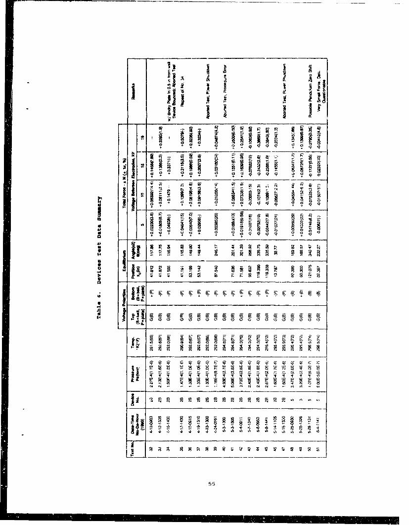
+U +

70;0 +i 0 I

ai cs OQO a+ + + ~9

II

7 N0 +ý eq 0q 09 00 90 ~ ~ u 4. 4. 4 . .* .

UU, l

N -M 0Y 0 0N~ ~ ) )

55

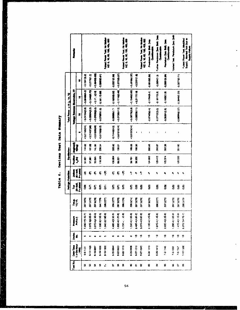
I -�

I. � �Ia

I' * A IA

�Aj �j_______ Iii ; j ii

git II lit I:1 � -� - 9

II!�IjIjilt--________ (I I �___ I- V - �II I I P

9+ *

J � I2: ________ § : :

U

4-. I Iii ___ _________

&&

�

�'9 9

� � - -

"4 - ('4 -

I * PC PC PC PC PC PC

Jf��I!!! Iii ill '� � �.

.6 .6 �

'�

I ____________ ____ j

56

JI y

9999,~ CO997

co a

Ut k j I t IR I. m w

'R' -. c

If r~ I2I0

4' w j w , w u

0 u0 0 00 0 0 0 0

N ~ IS a) N I- ) N 0 rm b

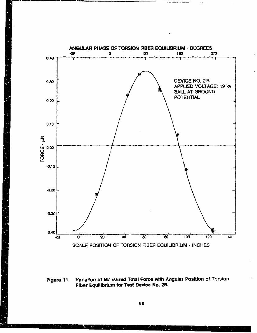
ANGULAR PHASE OF TORSON FIBER EQUIUBRIUM - DEGREES4)n 0 g0 160 270

0.40 '" i ti TWT -~l- W

0.30 DEVICE NO. 2 BAPPUED VOLTAGE: 19 kvSALL AT GROUND

0.20POTENTIA

0.10

zZL

S0.00a00u-

-0.10

-0-20 7/-0-30-

-0.40, - .... -. . . ,

-20 0 20 40 60 80 100 120 140

SCALE POSmON OF TORSION FIBER EQUIUBRIUM - INCHES

FIgure 11. Variaton of Me&isured Total Force with Angular Position of TorsionFiber Equilibrium for Test Device No. 2B

58

plotted in Figure 11 as a function of the scale positions of

equilibrium of the torsion pendulum. When the apparent

equilibrium position was changed from test to test, it was found

that the measured forces induced by identical electrical. driving

potentials varied periodically with an actual angular period of

180 degrees, and an apparent angular period of 360 degrees as

shown in Figure 11. This periodicity, if any, was expected since

the pendulum was configured with two test devices mounted in

tandem and 180 degrees (actual angles) apart.

The curve drawn through the data points (i.e., total

apparent force measures) represents a least squares fit of the

simple periodic function

F- a + bs in (O-C) (14)

where a is a phase angle, and the quantity (0-a) is referred to

as "angular phase of the torsion fiber equilibrium,, in Figure 11

and subsequent figures.

The use of a sine function to represent the angular

variation of the observed force may only be approximate, but

appeared to be adequate, and useful in this pr-ogram° The curYve

in Figure 11 is symmetric with respect to a negative, constant

force value, which lies somewhat below the zero force horizontal

line shown. This offset from zero indicates a non-zero value for

the parameter "all in the force representation given by

Equation (14). In turn, this implies the existence of a steady

torque component which acted in the same direction over the

complete test. Presumably, this steady torque component could

arise from the steady force of the Biefield-Brown type, so it is

of potential interest here. More will- be said later about this

steady torque com~ponent.

59

Once this apparent periodicity and approximate sine function

behavior was established,"*" it was found more convenient to

plot the force data as a function of sin(e - a) as shown in

Figure 12. The force values for 10 kV, 15 kV and 19 kV are shown

in Figure 12 for Test Device 2B, but those for 5 kV were omitted

because they are generally less reliable, and were not availablefor all of the device types tested. In the plot of Figure 12,each line through the force data points for a given drive voltage

intersects the vertical axis for the angular phase (0 - a) of

zero, at the offset value "a." In Figure 12, this offset

indicates a negative value of the steady force component 11a."

This corresponds to a force in the negative x direction, and for

Test Device 2B from the plate toward the ball.

The steady force component "a" can be determined from twomeasured forces at two known 6 values, or from three values of

the forces and 0 if a is treated as an unknown. Such a solution

can also be readily obtained with additional values using least

squares. The least squares approach emphasizes the force valuesnear the maxima and minima of the sine curve. It was, therefore,convenient to utilize force measures made near these extremes,

both to enhance the accuracy of the subsequent curve fits, and toreduce the number of tests required (as opposed to conducting

tests over the complete 360 degree range of the angular phase).

Subsequent tests were conducted with angular phases near the

maximum and minimum positions.

The force measures and corresponding curves for Test DeviceNo. lB observed in Tests Nos. 61 and 67 are shown in Figure 13.

Difficulties with pendulum zero shift, once the lower weight wasin position, rendered data for several of the intervening tests

**** Further confirmation was made using data from tests withtest device Nc. 5. Three values of a were determined and used:a - 74.82" for aest nevice Nos. 1B, 2B and 2C and 3; a - 61.23" forTest Device Nos. 4 and 5; and a - 52.56" for Test Device No. 6.

60

0.40 -- - " -' -- "T r-"'TTT----T-

0.30

19kv

0. 20

0.10 10 W

z L -. 0.0C- *- -- -*-

w

U I

-. 10o ..- /

DEVICE NO. 2 B-0.20 BALL AT GROUND POTENTIAL

-0.30

-0.40 . ILLLJL.!L1...

-1.0 -0.5 0 0.5 1.0

SINE OF ANGULtkR PHASE OF TORS!ON FIBER EQUILIBRIUM

Figure 12. Variation of Measured Total Force with Angular Phase of TorsionFiber Equilibrium for Test Device No. 2B

61

0.40 . ' I 'I

0.30 I~//

19 kV

0.20I

o~lo 10 WV0.10

:t 0.00 -

wU

.0.10

DEVICE NO. I B-0.20 BALL AT GROUND POTENTIAL

0.30

S.. .. I i,_ t. • ___.L__ .____1 . • _ J __L _J _.

-1.0 .0.5 , 0.5 1.0

SINE O" ANGULAR PHASE OF TORSION FIBER EQUIUBRIUM

Figure 13. Variation of Measured Total Force with Angular Phase of TorsionFiber Equilibrium for Test Device No. 1B

62

unreiiable. No such shifte were observed during Test Ncs. 61 or

67.

Similar force measures and curves for Test Device No. 3

observed in Test Nos. 84 through 87, are shown in Fi'qure 14.

Figure 15 indicates plots of the force measures and curves

for Test Device No. 4, as observed in Test Nos. 72 through 75.

Figure 16 shows plots of the forces and curves for Test

Device No. 5, as observed in Test Nos. 48 through 52, and 76

through 80. There was some question about stability of the

pendulum zero equilibrium in Test No. 50. The force levels were

very low in Test No. 51 and the force results in this case are

believed to be unreliable. Test Nos. 76 through 80 were

conducted later to confirm the early results and to ensure no

effects of pendulum zero shifts were present.

Figure 17 shows the force data and curves for Test Device

No. 6, as observed in Test Nos. 53 through 60, ind Test Nos. 70

and 71. The force levels in Test Nos. 53 and 57 appea:ed to be

anomalous for some unknown reason (perhaps because of undetected

pendulum zero shifts). Again Test Nos. 70 and 71 were conducted

later to supplement the early test results.

A data sumnary for the steady fo-ce component values for

tests shown in Figures 11 through 17 are given in Table 7,

together with their associated standard deviations determined

using least squares and the principle of propagation of

variance. 17

For completeness, the corr--nding force amplitudes (the

parameter "b" in Equation 14), for the test:3 anrd test devices ot

Table 7, are given in Table 8, together with their associated

standard deviations.

63

0.40 *

0.30

0.20 1 ikV

15kV

I -/0.10

S.010r -1

-0.20 DEVICE NO. 3

-0.30

-0.40 I I I . , . , ,

-1.0 -. 5 0 0.5 1.0

SINE OF ANGULA4R PHASE OF TORSION FIBER EQUILIBRIUM

Figure 14. Variation of Measured Total Force with Angular Phase oi TorsiGn Fiber

Equilibrium For Test Device No. 3

64

0.20 • r -"r -T - -- "-I • - •--

0.1519kV /

o~lo //15 kV * //

/ /0.1 ///// io kV~.

I // 10V0.05

z

0 -005U-

-0.107DEVICE NO. 4

-J.15

-0.20 •

-..L--_1 L L_._ - .__L -. _L J , 1 L....J-- ..-- L__._ I

-1.0 4,5 0 0.5 1.0

SINE OF ANGULAR PHASE OF TORSION FIBER EQUIUBRIUM

Figure 15. Variation of Measured Total Force w~th Angular Phase of TorsionFiber Equilibrium for Test Device No.0. 4

65

0.20 - - I T"I I T" T" I * u U I

0.15 I

19kV0.10

15 kV

0.0s _10 kV

z:1~0.00 -

Lu

-0.05

DEVICE NO. 5

-0.10

-0.15

-1.0 -0.5 0 0.5 1.0

SINE OF ANGULAR PHASE OF TORSION FIBER EQUIUBRIUM

Figure 16. Variation of Measured Total Force with Angular Phase of TorsionFiber Equilibrium for Test Device No. 5

66

0.40 i I i I 1'T' ifI t

0.30

19 kV0.20

o~lo _ 10 kV0.10

zZ- 0.00

Uj

cr_0LL

-0.10

-0.20DEVICE NO. 6

-0.30I

-0.40-1.0 -0.5 0 0.15 1.0

SINE OF ANGULAR PHASE OF TORSION FIBER EQUIUBRIUM

Figure 17. Variation of Measured Total Force with Angular Phase of TorsionFiber Equilibrium for Test Device No. 6

67

From earlier considerations in this report, it was noted

that the threshold of measurements with the torsion fiber force

measuring system was about 0.64 x 10"4 m (0.0025 in). This

together with the combined calibration parameter k (- 0.0796

dyn/in) given by Equation (12), indicates the measurement

threshold for residual forces is about + 0.002 gN (± 0.0002 dyn).

This value is relevant in considering the results given in

Table 7.

The results in Table 7 for Test Devices No. 4 and No. 5,

(i.e., symmetric ball devices, without and with a dielectric,

rpspectively) indicate therp was an average negative residual

force at 19 kV of

-0.0125 ± 0.0027 jLtN.

Further, for test devices No. 4 and No. 6 (i.e., the same

symmetric ball device without a dielectric, and a syn...etric plate

device without a dielectric) there was an average negative

residual force at 19 kV of

-0.0126 ± 0.0029 pN.

These two values, and correspondingly close average values for

each of the 15 kV and 10 kV conditions, show that the average

residual forces for these symmetric device types was very small,

was nearly independent of the actual type of symmetric device

tested, and did not appreciably depend on the presence or absence

of a dielectric. Further, these residual forces scale

approximately with the square of the applied voltage over this

10 kV to 19 kV range.

Accordingly to Brown, C53 these symmetric devices should

generate zero propulsive forces. The fact that they are not zero

68

Table 7. Residual Force Data Summary

Residual Force - &N + laDevice No. Device Configuration 19 kV 15 kV 10 kV

4 Sym. Ball, No Dim#. -0.0108 + 0.0004 -0.0067.4- 0.0002 -0.0C35 . 0.0001

Sym. Ball, with Diel. -0.0142 + 0.0023 -0.0081 + 0.0006 -0.0045 + 0.0007

1B Ball & Plate, No Diel. +0.0016 + 0.0028 -0.0001

2B Ball & Plate, with 1/4" -0.G243 + 0.0034 -0.0156 + 0.0022 -0.0074 + 0.0011Diel.

Bal & Plate, with 1/2" +0.0021 + 0.0021 -0.0004 + 0.0019 -0.0015 + 0.0011Diel.

4 Sym. Ball, No Diel. -0.0108 + 0.0004 -0.0067 + 0.0002 -0.0035 + 0.0001

6 Sym. Plate, No Diel. -0.0143 + 0.0025 -0.0094 + 0.0018 -0.0042 + 0,0011

Table 8. Force Amplitude Data Summary

Force Amplitude - ,N + loDevice No. Device Configuration 19 kV 15 10 kV

4 Sym. Ball, No Diel. 0.1992 + 0.0004 0.1241 + 0.0002 0.0542 + 0.0001

5 Sym. Ball, with Diel. 0.1698 + 0.0023 0.1055 + 0.0006 0.0478 -+ 0.0007

1B Ball & Plate. No D;el. 0.3316 0.2090 0.0905

2B Ball & Plate, with 1/4" 0.3596 +- 0.0044 0.2256 + 0.0029 00995 + 0.0015Diel.

3 BalI & Plate, with 1/2" 0.2999 + 0.0021 0.1880 + 0.0019 0.0827 + 0.0011Die!.

4 Sym. Ball, No Diel. 0.1992 + 0.0004 0.1241 + 0.0002 0.0542 + 0.0001

6 Sym. Plate, No Diel. 0.2975 + 0'0026 0.1840 + 0.0019 0.0811 + 0.0012

69

is of interest, since it suggests forces may have arisen from

some other cause.

It will also be noted that the residual forces given in

Table 7 for Test Devices No. lB (without a dielectric), No. 2B

(with a 1/4-in diameter dielectric) and No. 3 (with a 1/2-in

diameter dielectric) showed erratic results. All the residual

forces observed for Test Devices No. lB and No. 3 were near or

below the measurement threshold of ± 0.002 IN. As further

indication that theme values may only represent "noise," the sign

(or direction) and magnitude of the force did not appear to vary

with any particular functioral relationship to the driving

voltage.

The forces for device 2B were roughly twice the average

values indicated previously for the symmetric devices, were in

the same direction, and fell even further outside the rasurement

threshold limits than the forces observed for the symmetric

devices. It does not seem possible without further consideration

to reconcile the average residual force values observed for Test

Device No. 2B, with those observed for Test Devices Nos,

lB and 3. This issue will be noted later in the section on

Evaluation.

A final aspect of the device tests was concerned with the

measurement of electric current through the test devices by means

of the electrometers installed in the upper and lower conducting

fibers. The approach used was an attempt to overcome the

difficulties of measuring very small currents in the pico-ampere

range, at voltage levels of tens of kV, remotely, in a vacuum

chamber. This approach was useful, but was not nearly as

successful as we had hoped.

The electrometers were used during approximately a third of

the total tests, but measurements of device current were still

70

difficvlt tn obtain. The ei.ectrometer units turned out to be

quite sensitive to electrical "noise." within the chamber, even

though inside the chamber they were Etacah placed within a separate

stainless steel enclcsure, with one end covered vith aluminum

foil. Successful measurements of device current were made on

very few cf the tests conducted. A representative set of

absolute values of the average current through each test device

indicated by the electrometers is shown in Figure 18 for Test

Nos. 41 and 42. The test devices In these runs were ot type 2B--

a ball and plate unit with a 0.00635 m (0.250 in) diameter

acrylic rod between electrodes. The voltage polarity of the

plate electrode in Test No. 41 was negative, and in Test No. 42

it was positive; the ball electrode in each case was at the same

earth ground as the chamber wall. The direction of the current

in Test No. 41 is from the ball toward the plate, as expected,

and this direction is reversed in Test No. 42, si.n-e the pow

supply voltage was reversed.

VJ

Below ten kV, the average indicated current was about t

pico amperes (pA) total, or one pA per test device. This

corresponded to the approximate measurement threshold of the

electrometer system.

The variation of average current, i, throuqh device 2B WILun

applied potential difference, V, shown in Figure 18 can be

represented by the simple functional form

1 =av (a5 )

above the measurement threshold. This regression line, when

passed through the very limited number of points of Test 14as. 41

and 42 becomes

71

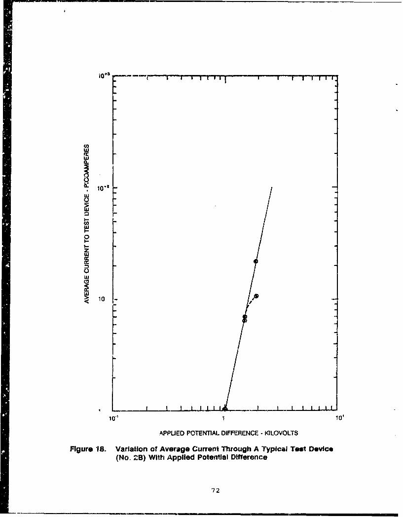
S 10+3

w

10-2* L

w r

C.)

w

> 10 .

10" 1 10'

APPLIED POTENTIAL DIFFERENCE - KILOVOLTS

Figure 18. Variation of Average Current Through A Typical Test Device(No. 2B) With Applied Potential Difference

72

Y-1.58X10-5 V4 79 (16)

where i is exAcL!ssed in pico amperes (pA) and V is in kilovolts

(kV). It will be observed that the value of current at 19 kV for

Test No. 42 is not well represented by Expression (16), even

though the currents at lower levels are.

The exponents in the preceding functional form are rather

sensitive to the actual data, and hence, to minor systematic

errors in the measured values. The values given, therefore,

should be considered only as representative. Scant data from

other tests suggest these absolute values may vary by perhaps a

factor of two or so from the values calculated using

Expression (16).

System Errors

Any measurement system is subject to errors, both random and

systematic, and the torsion fiber system used in this effort was

no exception.

The main random errors were associated with the actual---and

in some cases only a suspected---zero shift of the equilibrium

position of the torsion pendulum. This zero shift was not

observed during the early boundary effects tests, but became

apparent after Test No. 62. A problem was suspected with the

force measurements during Test Nos. 50 and 53, but routine

observations of the fiber tensioning mass at the bottom of the

chamber showed no apparent motion or change in angular position

of this mass with respect to the conducting platform on which it

rested. Later, it become apparent that mechanical vibration,

presumably induced by the backup mechanical vacuum pump, was

causing the tensioning mass to shift its angular position

73

slightly after the mass was lowered onto the platform. This

shift was not consistent, and apparently caused the fiber to

twist sufficiently to alter the effective calibration value

slightly. This problem was addressed during Tests Nos. 63

through 66 and was overcome by reducing the vibration level. The

absence of such angular shifts was checked subsequently by noting

the equilibrium positions of the pendulum before and after

lowering the tensioning mass. As a result of this finding,

selected tests of device Nos. 5 and 6 were repeated to confirm

earlier findings.

The main systematic effects encountered were associated with

electrostatically induced boundary forces which affected the

behavior of test devices mounted. on the torsion pendulum.

Initially it was unknown if all of these effects could be

accounted for, or if some would remain as systematic errors, or

if Brown-type residual forces could be identified as r.-rt of the

observed effects.

As noted earlier, considerable effort was expended to

minimize the boundary effects, but it became apparent that even

with the application of conductive shields placed inside the

vacuum chamber an appreciable induced force was present. This

force acted on both the symmetric and asymmetric types of test

devices during test runs. Also, this force was found to depend

on the angular position of the test devices about the chamber

vertical axis (which is indicated, equivalently, by the angular

position of the zero torsion equilibrium condition of the

pendulum) as a near periodic function which could be represented

mathematically by Equation (14), [i.e. F=a+b sin (8-a)].

A force contribution with a dependence of the form

"b sin (6-a)" can arise from electrostatically induced charges on

the walls of t*' chamber if the axis of the torsion fiber is

74

parallel to, but offset from, the axis of cylindrical symmetry

for the chamber.

The prospect of the fiber axis not being coincident with the

chamber axis was rather likely, and a separation distance between

the axes up to perhaps 5 mm (0.2 in) was possible.***** It is

believed that such an axial offset of the torsion fiber was

responsible for the approximate variation of the force amplitude

with the sine of the angular phase (0-a) of the torsion fiber

equilibrium position.

The parameter "a" in Equation (14), represents an offset

component of the total observed force, from zero. A non-zero

value of "a" implied, at first sight, the existence of a steady,

residual force component (in addition to the variable component

noted above), which acted in the same direction over the complete

set of torsion equilibrium positions observed, for a given test

device type. As noted earlier, this steady force component. could

presumably arise from a steady force of the Biefield-Brown type.

However, it is believed that a conventional explanation for this

apparent steady force component is more likely the correct one,

and this apparent force--rather that a Biefield-Brown type of

force--was responsible for the non-zero values of "all that were

determined from observations.

This argument applies specifically to the tests and test

results in which symmetric test devices were used, such as test

device Nos. 4, 5 and 6 indicated in Table 2, and to the

corresponding test results given in Table 7.

The vacuum chamber used was not of precision constructionand the centers of the available top and bottom access ports inwhich the fibers were mounted could have been slightly off thechamber axis. Direct measurements did not indicate such an offset,but accurate measures within the chamber were difficult, andmeasures on the outside of the chamber were precluded because of asurrounding (empty) water jacket.

75

Experimentally, the equilibrium positions of the torsion

pendulum were observed only over a 180" angular range, rather

than over 360' of a true angular period. The 180" angular range

used was expected to represent the effective angular period,

since the pendulum was configured with two test devices mounted

in tandem and 180" apart. Indeed, this would be 1he case if

there were complete symmetry in the construction of the device

holder and test devices. However, if the two test devices were

held at only slightly different distances from the torsion fiber

axis, and if the fibur axis was simultaneously offset from and

parallel to the chamber axis, as shown in Figure 19, then an

asymmetry effect would occur as indicated in Figure 20.

The device support orientation direction in Figure 19

corresponds to an equilibrium position 'l0ol of the torsion

pendulum. The positions labelled 0 through 8 correspold to a

sequence of positions toward which the device support orientation

arrow would point if the pendulum equilibrium position were

changed in equal steps over the complete angular period of 360'.

This same angular position sequence is indicated in Figure 20b

and along the curve in Figure 20a. In Figure 20a, the curve

represents schematically the apparent force that would be

measured using a torsion fiber and the two tandem mounted

symmetric test devices, as in the tests conducted in this

program.

It will be noted from Figure 20a that the apparent force can

be viewed as if it exhibited symmetry about the zero force axis

in two regions (of 180" each), labelled "symmetric #1" and

"symmetric #2." As shown, the maximum force amplitudes in

symmetric #1 region are larger than those in symmetric #2. The

curves in each region are not identically simple sine curves, but

if the maximum amplitude difference between the regions is smal1,

the curves can ,c zlýsely approximated by sine curves.

76

DEVICE NO. 1

CHAMBER AXIS

FIBER AXIS

DEVICE NO. 2

2

-7"

7% 5

-DEVICE SUPPORT ORIENTATION

Figure 19. Orientations of Asymmetric Device Support Structure and Fiber AxisOffset

77

h0

t 0 1805

2 4c 2 S4mrnetrc #2

(a)

73F'i Asymmetric Asymmetric 3

Type I Type II

21 3

(b)0 48

7 -6

Figure 20. Asymmetry Effect from Device Support Structure and Offset FiberAxis

78

Alternately, the apparent force in Figure 20a can also be

viewed as if it exhibited asymmetry about the zero force axis in

two other regions, designated "asymmetric type I" and "asymmetric

type II." These regions are merely shifted 90' in angular phase

of the torsion fiber equilibrium position, from the symmetric

regions. Again these curves in each region are not identical

simple sine curves, but can be closely approximated by sine

curves, each with an apparent steady force component such as "a"

in Equation (14).

If tests were conducted within the 180" region corresponding

to "asymmetric type I," then negative values of "a" would be

determined from force observations (as was found in this

program). In the "asymmetric type II" region, positive values of

"a" would be determined. In both of the symmetric regions the

values of "a" would be essentially zero.

The prospect of the two test devices mounted on the support

holder not being at the same distances from the fiber axis is

certain. Care was taken to fabricate the small, 4.75 mm

(0.187 in) diameter aluminum tubing support arms (shown in

Figure 3 using a mechanical jig). Even so, when assembled, the

moment arm to one device was 9.807 cm, and to the other was

9.750 cm, giving an average of 9.778 cm, and a difference of

0.057 cm (0.025 in). This difference amounts to only 0.58

percent of the average arm length. As such, it was not initially

recognized as significant, and no attempt was made to reduce this

moment arm difference. The average offset force determined for

symmetric test devices Nos. 4 and 5 was -0.0125 gN (from Table

7); for the moment arm difference of 0.57 mm, this gives a value

of 0.022 gN/mm. A similar result for the force amplitude of

these same devices was 0.1845 gN (from Table 8), which for an

assumed axial offset of 5.0 mm gives a value of 0.037 gN/mm.

While these values are not identical, they are certainly of the

same order, and tend to support the belief that the difference in

79

moment arm lengths of the test device support structure is the

basis for the steady force component "a" observed in the

symmetric device tests noted in Tables 6, 7 and 8.

Evaluation

The magnitudes of the total and residual force measurements

need to be compared with estimates of the magnitudes of the

electric wind and the ion propulsion effects to determine if the

latter effects can account for any of the observed forces.

The total force measurements made under high vacuum

conditions near 1.33x10"4 Pa (l.Oxl0"6 torr) were not expected to

be influenced by electric wind effects, because the mean free

path in N2, or air, under these conditions is of the order of

50 m. This is many times the separation distance of A& device

electrodes, and, indeed, is also many times the largest. linear

dimension within the vacuum chamber used. The molecular density

is simply not large enough to cause the entrainment of air

molecules, and to cause electric wind effects under these

conditions.

The magnitude of the ion propulsion effect depends on the

size of the excess diffusion current emitted by one electrode

over that collected by a second electrode within a test device.

This excess or differential current was indicated by the

electrometer in the propulsion device tests, was generally quite

variable, and was not always consistent in sign or direction.

Generally, these currents were well below about 100 pA (except

during breakdown) during the tests run in a high vacuum. Thus,

ixl01" A represents an approximate upper bound on the current

expected to contribute to the ion propulsion effect in most of

the tests.

80

A general expression for the force, F, expected from such an

electrostatic thruster is given by Sutton and Ross[83:

F- I 2V4 (17)e

where

F= accelerating force, N

I= propelling current flow, A

V= accelerating potential difference, V

IA= mass of accelerated particle, kg

e= charge per particle, C.

For a threshold current of I=10"'0 A, V= 19 kV and e= 1.60x10" 19 C,

equation (17) gives

F- 48.7 VIN.

If the accelerated particles were all electrons, protons, or

aluminum ions (single charge), the corresponding maximum forces

would be:

electrons: = 9.11 X 10,31 kg

F = 4.65 x 10-14 N = 4.65 x 10 9 dyn

protons: I = 1.672 x 10-27 kg

F = 1.99 x 1 0"Z N = 1.99 x I07 dyn

aluminum ions: g = 26.98 x IT" kg/AMU = 44.8 x 10-27 kg

F = 1.03 x 10'11 N = 1.03 x 10,6 dyn.

The force per device would be one-half of each of these values.

81

These estimates assume that all the ion current would actcollectively to propel each device in one direction. These forcevalues per device are at most less than 1/400 ot the force

measurement threshold value of 2x10l9 N (0.0002 dyn).

Here, these estimates for ion propulsion effects are

negligible.

This leaves a remaining question regarding reconciliation ofthe average residual force values observed and noted in Table 7

for Test Device No. 2B, with the values observed for Test Device

Nos. 1B and 3.

In the previous discussion !f systematic effects forsymmetric test devices, it was argued that the observed residual

forces in these tests were almost certainly artifacts associatedwith a combination of systematic errors. These error,- included:

an off-axis fiber; the construction asymmetry of the device

bolder; and the employment of an assumed 180" angular periodicityof pendulum equilibrium positions, rather than the complete 360Q

angular period. While only symmetric test devices wereconsidered, it is expected that a similar effect would hold forasymmetric test devices, such as those used in Test Nos. 1B, 2B

and 3. The residual force values determined for these tests withasymmetric devices, might not be exactly the same as thoseexperienced with the symmetric devices. However, on the basis of

the sytimetric device tests with and without a dielectric, onewould expect nearly identical force values to be observed for

Test Devices Nos. 1B, 2B and 3. Since we became more aware of

potential errors as the test program proceeded, and we paidgreater attention to minimizing them, we now give greater

credence to the residual force results obtained for Test Device

Nos. 1B and 3, than for Test Device No. 2B. Full reconciliation

c.annot be givei., .ut we tend to discount the residual force

results obtained for T*-t Device No. 2B as being erroneous.

82

Anomalies

Near the end of this experimental program, we briefly

examined the force generation effects with pulsed fields, which

had a peak voltage of 19 kV. Test Nos. 56, 59, 62, 68 and 69

were conducted in this manner, using pulse repetition rates of

10, 60, 150, 400 and 600 Hz. Generally, no motion of the test

devices was observed, except in Test No. 69 where a very small,

but detectable motion was seen. For an input voltage of 19 kV

during this test, the apparent force was about 0.007 4N (which is

just above the force measurement threshold of 0.002 WN) and is

,iot considered significant.

Two tests, Nos. 81 and 82 were conducted to examine the

effect on forces generated by test devices where a dielectric wasused which had a significantly larger dielectric constant than

,possessed by acrylic. Each of these two tests used test devices

of type 2C with a ceramic piezoelectric material of lead titanate

lead zirconate.* .... This material had a dielectric constant

of about 1750 along the length of the cylinder. The direction of

dielectric poling was also along the length of the cylinder. The

force generation results for both of these tests appeared

anomnalous.

A computer plot of the direct torsion pendulum positions for

anomalous Test No. 81 is shown in Figure 21. The first set of

deilections for the driving voltage steps of 5, 10, and 15 kV

gave negative displacements, which appeared normal. When thevoltage was increased to 19 kV, a slow pulsing breakdown was

detected on the 0-2 mA meter mounted on the power supply. Afterone full swing of the pendulum, the voltage level was reduced

S..*.. This material, designated channel 5500, was produced byChannel Products. Inc., 7100 Wilson Mills Road., Chesterland, Ohio44026.

83

6z

00

U.

0 L

01 W.

IU 0 ----

ov.

0

LU

C%

Go) 0QOE

wNMO~dl

I- 84

again to 15 )rV. At .5 kV the displacements again stabilized, but.

had shifted from their original position before the breakdown

pulse. The first set of voltage steps was completed by returning

the valtage again to zero.

A second set ot the same voltage steps was then started, arid

the pendulum displacements at 5, 10 and 15 kV were similar to

those of the first set. There was an indication of minor pulsing

breakdown at 15 kV for this set. This set was completed by

returning the voltage to zero. This pendulum position at this

new zero voltage setting was nearly the same as for the previous

zero.

A third voltage set was then initiated, again using steps of

5, 10, and 15 kV. This time at 15 kV, more significant pulsing

breakdown was experienced and the pendulum positions began to

move toward larger numerical values (i.e., in the positive

direction) while the pulsing continued. After a few oscillations

of the torsion pendulum, the driving voltage was increased to

19 kV, and an even greater, slow pulsing breakdown occurred.

While this pulsing breakdown continued, the torsion pendulum

began to move so the positions of its center of oscillation

increased in value. Each point indicated in the position plots

in Figure 21, represent the average pendulum position during one

swing (one-half of a complete oscillation). The pendulum

positions continued to change in the positive direction, opposite

to the "normal" displacements from zero observed earlier for

voltage steps of 5, 10 and 15 kV. These position changes

continued to occur in the same direction for ten swings, or about

4.4 min, and then tended to reverse for two more swings (0.9 min)

as if there had been an "overshoot" of position.

It is important to note that the observed rate of change of

position in this case was rather slow, and it occurred with a

85

"wconstant" driving voltage applied to the test device

(recognizing that the voltage may have fluctuated some during the

breakdown pulses). This position change was not the same as a

free ralease of the torsion pendulum, which might be expected to

allow the pendulum to swing with increased amplitudes. The

positions observed represent the positions of the centers of

swing of the pendulum. Further, under normal conditions where

breakdowns did not occur, the pendulum positions were usually

almost constant for successive swings, and when the driving

voltages were changeC the positions typically responded to the

new levels in one or two swings.

The driving voltage was then returned from 19 kV to zero.

The pendulum position again Increased for one swing in the

positive direction. During the thirteen subsequent swings

(5.7 min) the pendulum slowly returned to a "zero" position, very

nearly the same as the zero position at the start of tl:is voltage

set.

A final voltage set was Itnn run, and at 15 kV a pulsing

breakdown again occurred; this was accompanied by a positive

pendulum displacement as for the previous 15 kV voltage step.

The voltage was then increased to 19 kV, large additional

breakdowns occurred, ard a small negative displacement jump was

observed. This time, however, the large positive displacement

shift observed previously was not repeated, and the final zero

voltage step did not return the pendulum position to its value at

the beginning of this last voltage set.

A complete plot of the torsion pendulum for Test No. 82 is

shown in Figure 22. For this test, the first voltage step

applied was 19 kV, to achieve pulsing voltage breakdowns within

the test devices similar to those developed during Test No. 8].

86

0

0 00 E- 0

0C'M - LL

00a

zE

uuJ

~~0

0 0

0

m cc cc4" cn e

-0* o* -* .0 .0; -0 0

IN3"3V~dS0

- - 287

Such breakdowns did occur and the rate at which they pulsed was

variable during the 11.7 min while the applied voltage was

maintained (relatively) constant. Rather sizeable changes in

pendulum position opposite to the "normal" direction were

observed during this first 19 kV voltage step, similar (but less

consistent) than those observed in Test No. 81.

Finally, the applied voltage was returned to zero, and the

pendulum position assumed a new zero reading rather than the

original reading.

Next, a second 19 kV vcltage level was applied. In this

case, the breakdown pulses were slow for the fir'st two pendulum

positLons plotted. They then occurred faster and the pendulum

position began moving toward larger values. After four such

swings, the pulse rate again slowed for a swing, the prndulum

position decreased and then finally stabilized after e few more

swings.

The voltage was again returned to zero, and the pendulum

position also returned to essentially the same zero as it was for

the previous cycle.

A third voltage level of 39 kV was applied, and similar, but

less pronounced pendulum position changes toward lar'c.er values

were observed. The voltage was then returned to zero, and the

pendulum position also returned to the same zero position.

A fourth voltage level or 18 kV was applied and the

breakdown pulsing rate was fast at first, .hen slowed after the

first four swings. T'he pendulum positions responded just as in

the earlier 19 kV case where the polsing rate was noted. When

the voltage level was changed to zero, the pendulum position also

returned to (nar) the sam~e position zero.

88

The final voltage level applied was 15 kV, and the

associated pendulum position behavior was similar to that for the

previous voltage step.

The force behaviors in Test Nos. 81 and 82 remain

anomalous---compared with the results observed when no breakdowns

were occurring across the dielectric in the test devices. From

visual observations, it was noted that the electrical breakdowns

were occurring in the vicinity of the dielectric. These were

probably breakdowns over the surface of the dielectric rods,

rather than through their interior, but this could not be

distinguished by visual observations.

Key observations made during these tests can be summarized

as follows:

The anomalous force was associated with the occurrence

of electrical breakdowns over (or through) the

piezoelectric dielectric between electrodes held at a

potential difference of about 19 kV.

The anomalous force seemed to increase as the rate of

breakdown pulsing increased, even though the observed

pulsing rates were no more than a few pulses per

second.

The anomalous force acted in a direction opposite to

the direction of the conventional electrostatically

induced boundary force for these two tests (this may

not be true in general). This suggests that the

anomalous force is not due to electrostatic charges

induced, generated, or somehow caused to appear on the

test devices, since the boundary type forces arising

from the presence of charge are independent of the sign

of the charge.

89

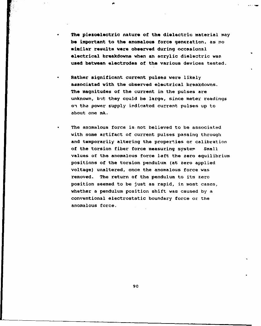
* The piezoelectric nature of the dielectric material maybe important to the anomalous force generation, as no

similar results were observed during occasional

electrical breakdowns when an acrylic dielectric was

used between electrodes of the various devices tested.

Rather significant current pulses were likely

associated with the observed electrical breakdowns.

The magnitudes of the current in the pulses are

unknown, but they could be large, since meter readings

on the power supply indicated current pulses up to

about one mA.

* The anomalous force is-not believed to be associated

with some artifact of current pulses passing through

and temporarily altering the properties or calibration

of the torsion fiber force measuring system Small

values of the anomalous force left the zero equilibrium

positions of the torsion pendulum (at zero applied

voltage) unaltered, once the anomalous force was

removed. The return of the pendulum to its zero

position seemed to be just as rapid, in most cases,

whether a pendulum position shift was caused by a

conventional electrostatic boundary force or the

anomalous force.

90

CONCLUSIONS

The following conclusions have been reached based on the

investigations of the Biefield-Brown effect conducted on this

project:

1. Direct experimental results show that under high vacuum

conditions, with air pressures in the approximate range of

1.33x10"3 Pa (l.0xl0"5 torr) to 6.3x10"5 Pa (5.0 x 10"7 torr),

no detectable propulsive force was electrostatically induced

by applying a static potential difference up to 19 kV

between test device electrodes, either with or without a

spatial divergence of the electric field and energy density

within that field. The minimum detectable force in these

experiments was about 2x10*9 N.

2. The electrostatically generated propulsive force, which was

claimed to exist by T.T. Brown for test devices driven by

steady electrostatic potential differences between the

device electrodes, under high vacuum conditions "when there

was no vacuum spark," was not observed. If such a force

still exists and lies below the threshold of measurements in

this program, then the force may be too small to be

attractive for many, if not most, space propulsion

applications.

3. The boundary effects associated with making

electrostatically induced propulsive force measurements,

such as those explored under this program, are severe inside

a vacuum chamber of small or moderate size with conductinq

walls (and presumably also with dielectric walls). Great

care must be exercised in achieving adequate symmetry in the

complete measurement configuration so that sufficiently

small force levels can be detected and measured.

91

Experimental difficulties are exacerbated by the need to

conduct tests remotely within a chamber under a high vacuum.

4. Steady electrostatic potential differences somewhat higher

than 19 kV (up to 33 kV) were occasionally obtained during

the tests, but there was no indication that any significant

nonlinearities were induced in any of the test devices which

would cause significant propulsive forces to develop using

such techniques.

5. Anomalous propulsive force generation results were obtained

during two tests with " ball and plate type of test device

when these electrodes were separated by a high dielectric

constant, ceramic piezoelectric material, and only when

electrical breakdowns occurred between the electrodes. The

magnitude of the anomalous force observed tended $a increase

as the rate of breakdown pulsing increased, even O'h6ugh the

observed pulsing rates were no more than a few pulses per

second.

92

RECOMMENDATIONS

As a result of this investigation, it is recommended that

the investigation of propulsive forces generated on test devices

by the action of abrupt electrical breakdown (and possibly other

type) pulses applied to piezoelectric and/or select dielectric

materials be continued. The purpose of this activity would be to

further explore and verify the existence of the "anomalous force"

noted in this report. Such investigations should initially be

conducted without the complication of operating within a vacuum

chamber. Verification of promising results in a vacuum

environment will be necessary at the appropriate time. Further

consideration needs to be given to techniques for measuring such

anomalous forces directly, since torsion fiber based systems may

not be appropriate.

It is also recommended that no further effort be expended on

DC voltage driven propulsive force generation systems of the type

examined under this program.

93

REFERENCES

1. R.L. Talley, 21st Century Propulsion Concept, AFAL-TR-88-031, April 1988, Final Report on AF Contract No. F04611-87-C-0058 with Veritay Technology, Inc., P.O. Box 305, EastAmherst, NY 14051.

2. R.L. Talley, 21st Century Propulsion Concept. Final Reporton NYS Contract No. SBIR (88)-166 of NYS Science andTechnology Foundation with Veritay Technology, Inc., P.O.Box 305, East Amherst, NY 14051.

3. D.E. Gray (ed.), American I~stitute of Physics Handbook,McGraw-Hill Book Cc., New York, 1957, pp.2-61, 3-78, 3-80.

4. A. Elliott and J.M. Dickson, Laboratory Instruments: TheirDesign and.Applicatin, Chemical Publishing Co., New York,1960.

5. T.T. Brown, Electrokinetic Apparatus, U.S. Patent 3,187,206June 1, 1965.

6. A.A. Andronov and C.E. Chaikin, Theory of Oscillatiogn,Princeton Univ. Press, Princeton, 1949.

7. W.E. Deming, Statistical Adjustment of Data, DoverPublications, New York, 1964, (See especially Sections 20and 62).

8. G.P. Sutton and D.M. Ross, Rocket Propulsion Elements, 4thed., John Wiley and Sons, New York, 1976, p 481.

94