R792 Finite Element Analysis of Plastic Bending of Cold ...

FINITE ELEMENT ANALYSIS OF PLASTICBENDING OF COLD-FORMED RECTANGULAR

HOLLOW SECTION BEAMS

Research Report No R792October 1999

Tim Wilkinson BSc BE MAGregory J. Hancock BSc BE PhD

The University of SydneyDepartment of Civil Engineering

Centre for Advanced Structural Engineering

SYNOPSIS

This report describes the finite element analysis of rectangular hollow section (RHS) beams, tosimulate a series of bending tests. The finite element program ABAQUS was used for theanalysis. The main aims of the analysis were to determine trends, to understand the occurrenceof inelastic instability, and to attempt to predict the rotation capacity of cold-formed RHS beams.

The maximum loads predicted were slightly lower than those observed experimentally, since thenumerical model assumed only three distinct material properties in the RHS. In reality, thevariation of material properties around the RHS cross-section is gradual.

Introducing geometric imperfections into the model was essential to obtain results that were closeto the experimental results. A perfect specimen without imperfections achieved rotationcapacities much higher than those observed experimentally. Introducing a bow-out imperfection,constant along the length of the beam, as was measured (approximately) experimentally, did notaffect the numerical results significantly. To simulate the effect of the imperfections induced bywelding the loading plates to the beams in the experiments, the amplitude of the bow-outimperfection was varied sinusoidally along the length of the beam. The size of the imperfectionshad an unexpectedly large influence on the rotation capacity of the specimens. Largerimperfections were required on the more slender sections to simulate the experimental results.The sensitivity to imperfection size increased as the aspect ratio of the RHS decreased.

The finite element analysis determined similar trends as observed experimentally, namely that therotation capacity was a function of both the flange and web slenderness, and that for a givenaspect ratio, the relationship between web slenderness and rotation capacity was non-linear, andthe slope of the line describing the relationship increased as the web slenderness decreased.

KEYWORDS : Cold-formed steel, hollow sections, RHS, finite element analysis, ABAQUS,plastic design, bending, rotation capacity, local buckling.

2

Science can amuse and fascinate us all, but it is engineering that changes theworld.

Isaac Asimov, in Isaac Asimov's Book of Science and Nature Quotations, 1988.

Email the authors of this research report:[email protected]@civil.usyd.edu.au

Please visit the Department of Civil Engineering web site athttp://www.civil.usyd.edu.au

3

CONTENTS

1 Introduction . . . . . . . . . . . . . . . . . . . . . . . . . . . . . . . . . . . . . . . . . . . . . . . . . . . . . . 51.1 The Bending Behaviour of Steel Beams . . . . . . . . . . . . . . . . . . . . . . . . . . . . 51.2 The Need for Finite Element Simulation . . . . . . . . . . . . . . . . . . . . . . . . . . . . 7

2 Development of the Finite Element Model . . . . . . . . . . . . . . . . . . . . . . . . . . . . . . 92.1 Physical Model . . . . . . . . . . . . . . . . . . . . . . . . . . . . . . . . . . . . . . . . . . . . . . . 92.2 Symmetry and Boundary Conditions . . . . . . . . . . . . . . . . . . . . . . . . . . . . . . 102.3 Choice of Element Type . . . . . . . . . . . . . . . . . . . . . . . . . . . . . . . . . . . . . . . 122.4 Loading . . . . . . . . . . . . . . . . . . . . . . . . . . . . . . . . . . . . . . . . . . . . . . . . . . . 152.5 Pre and Post Processing . . . . . . . . . . . . . . . . . . . . . . . . . . . . . . . . . . . . . . . 162.6 Material Properties . . . . . . . . . . . . . . . . . . . . . . . . . . . . . . . . . . . . . . . . . . . 182.7 Residual Stresses . . . . . . . . . . . . . . . . . . . . . . . . . . . . . . . . . . . . . . . . . . . . 212.8 Mesh Refinement . . . . . . . . . . . . . . . . . . . . . . . . . . . . . . . . . . . . . . . . . . . . 222.9 Geometric Imperfections . . . . . . . . . . . . . . . . . . . . . . . . . . . . . . . . . . . . . . 24

2.9.1 “Bow-out” Imperfections . . . . . . . . . . . . . . . . . . . . . . . . . . . . . . . . 242.9.2 Continuous Sinusoidal Imperfection . . . . . . . . . . . . . . . . . . . . . . . . 282.9.3 Single Sinusoidal Imperfection . . . . . . . . . . . . . . . . . . . . . . . . . . . . 332.9.4 Comparing Rotation Capacities . . . . . . . . . . . . . . . . . . . . . . . . . . . . 352.9.5 Imperfection Size . . . . . . . . . . . . . . . . . . . . . . . . . . . . . . . . . . . . . . 362.9.6 Effect of Scale Factor . . . . . . . . . . . . . . . . . . . . . . . . . . . . . . . . . . . 452.9.7 Effect of Steel Grade . . . . . . . . . . . . . . . . . . . . . . . . . . . . . . . . . . . . 46

3 Simulation of the Bending Tests . . . . . . . . . . . . . . . . . . . . . . . . . . . . . . . . . . . . . 513.1 General . . . . . . . . . . . . . . . . . . . . . . . . . . . . . . . . . . . . . . . . . . . . . . . . . . . . 513.2 Results . . . . . . . . . . . . . . . . . . . . . . . . . . . . . . . . . . . . . . . . . . . . . . . . . . . . 513.3 Discussion . . . . . . . . . . . . . . . . . . . . . . . . . . . . . . . . . . . . . . . . . . . . . . . . . 56

4 Parametric Study . . . . . . . . . . . . . . . . . . . . . . . . . . . . . . . . . . . . . . . . . . . . . . . . . 58

5 Conclusions . . . . . . . . . . . . . . . . . . . . . . . . . . . . . . . . . . . . . . . . . . . . . . . . . . . . . 595.1 Summary . . . . . . . . . . . . . . . . . . . . . . . . . . . . . . . . . . . . . . . . . . . . . . . . . . 595.2 Further Study . . . . . . . . . . . . . . . . . . . . . . . . . . . . . . . . . . . . . . . . . . . . . . . 60

6 Acknowledgements . . . . . . . . . . . . . . . . . . . . . . . . . . . . . . . . . . . . . . . . . . . . . . . 61

7 References . . . . . . . . . . . . . . . . . . . . . . . . . . . . . . . . . . . . . . . . . . . . . . . . . . . . . . 62

8 Notation . . . . . . . . . . . . . . . . . . . . . . . . . . . . . . . . . . . . . . . . . . . . . . . . . . . . . . . . 64

Appendices . . . . . . . . . . . . . . . . . . . . . . . . . . . . . . . . . . . . . . . . . . . . . . . . . . . . . . . . . . . . 66A Parametric Study in the F. E. Analysis of Cold-Formed RHS Beams . . . . . . 67

A.1 Introduction . . . . . . . . . . . . . . . . . . . . . . . . . . . . . . . . . . . . . . . . . . 67A.2 Effect of Yield Stress . . . . . . . . . . . . . . . . . . . . . . . . . . . . . . . . . . . 68A.3 Effect of Strain Hardening and Yield Plateau . . . . . . . . . . . . . . . . . . 74A.4 Effect of Corner Radius . . . . . . . . . . . . . . . . . . . . . . . . . . . . . . . . . 79A.5 Effect of Beam Length . . . . . . . . . . . . . . . . . . . . . . . . . . . . . . . . . . 83A.6 Effect of Welding . . . . . . . . . . . . . . . . . . . . . . . . . . . . . . . . . . . . . . 85A.7 Conclusion . . . . . . . . . . . . . . . . . . . . . . . . . . . . . . . . . . . . . . . . . . . 90

B Tensile Coupon Tests and Stress Strain Curves . . . . . . . . . . . . . . . . . . . . . . 91C Imperfection Measurements . . . . . . . . . . . . . . . . . . . . . . . . . . . . . . . . . . . 101

4

[blank page]

5

1. INTRODUCTION

Plastic design of statically indeterminate frames can lead to higher ultimate loadswith associated higher deformations, when compared with traditional elastic designmethods. Cold-formed rectangular hollow sections (RHS) have properties such ashigh torsional stability which result in less bracing, and which could be exploitedbeneficially in plastic design. However, most current structural steel designstandards do not permit plastic design for structures constructed from cold-formedRHS as a result of lack of knowledge in this area.

This report forms part of a research project whose aim is to show that cold-formedRHS are suitable for plastic design. Previous reports have examined theexperimental behaviour of cold-formed RHS beams (Wilkinson and Hancock 1997),connections (Wilkinson and Hancock 1998a), and frames (Wilkinson and Hancock1999). This report describes a series of finite element analyses to supplement thetests on RHS beams described in Wilkinson and Hancock (1997).

The main aim of the finite element analysis is to investigate the sensitivity of therotation capacity of RHS beams to geometric imperfections and material properties.Cold-formed steel structural members have distinctly different residual stresses andgeometric imperfections from hot-formed RHS beams. Hot-formed RHS beamshave been investigated by previous research (Stranghöner 1995; Stranghöner et al1994; and Stranghöner and Sedlacek 1996).

1.1 THE BENDING BEHAVIOUR OF STEEL BEAMS

Figure 1 shows the cross section of a typical RHS and defines the dimensions d, b,t, and r (depth, width, thickness, and external corner radius) of the section. Whene

a transverse load (P) is applied to a steel beam, as shown in Figure 2, there is abending moment (M), which induces curvature (�) in the beam.

In bending, the beam can exhibit several different types of structural behaviourassociated with local instability. Figure 3 illustrates the various types of behaviourof different classes of steel beams constructed from cold-formed RHS. In Figure 3,the moment is normalised with respect to the plastic moment (M ), and the curvaturep

(�) is normalised with respect to � , where � = M /EI, and EI is the elastic flexuralp p p

rigidity.

If the section can reach the plastic moment, then the rotation capacity (R) is ameasure of rotation between reaching M and the point where the moment fallsp

below M . R is defined as �/� - 1, where �/� is the dimensionless curvature atp p p

which the moment drops below M . The decrease in moment is usually associatedp

with an inelastic local buckle.

d

b

t

Web

Flange

Adjacent 1

Adjacent 2

Corner

Weld

Opposite

re

P

MM

0

0.2

0.4

0.6

0.8

1

1.2

1.4

0 1 2 3 4 5 6 7 8 9

Non Dimensional Curvature (κ/κp)

Non

Dim

ensi

onal

Mom

ent (M

/Mp)

Compact (Class 1) Behaviour:

M max > M p, R > 4

Non-Compact (Class 2) Behaviour:

M max > M p, R < 4

Slender (Class 4) Behaviour:M max < M y

Non-Compact (Class 3) Behaviour:

M y < M max < M pR = κ/κp - 1

6

Figure 1: Typical Rectangular Hollow Section

Figure 2: Beam Under Transverse Load

Figure 3: Typical Bending Behaviour of RHS Beams

7

A “compact” or “Class 1” section is deemed suitable for plastic design. Such asection can reach the plastic moment, and then rotate further maintaining M for ap

suitably large rotation, which would allow for moment redistribution in a staticallyindeterminate structure.

The most common method of classifying sections is by comparing the web andflange slenderness to appropriate slenderness limits. In the Australian Standard AS4100 (Standards Australia 1998) the web and flange slenderness are defined as �w

= (d-2t)/t × �(f /250) and � = (b-2t)/t × �(f /250) respectively.y f y

1.2 THE NEED FOR FINITE ELEMENT SIMULATION

Previous parts of this research project (Wilkinson and Hancock 1997, 1998b,Wilkinson 1999) described tests on cold-formed RHS beams to examine the Class 1flange and web slenderness limits. Forty four (44) bending tests were performed on16 different specimens. Some specimens of the same type were tested more thanonce to examine the effect of loading method. The main conclusions of the testseries were:(i) Some cold-formed RHS which are classified as Compact or Class 1 by

current steel design specifications do not maintain plastic rotations consideredsufficient for plastic design.

(ii) The current design philosophy, in which flange and web slenderness limitsare prescribed independently, is inappropriate. An interaction formula isrequired, and simple formulations were proposed for RHS.

The sections represented a broad range of web and flange slenderness values, butit would have been desirable to test a much larger selection of specimens. However,a more extensive test program would have been expensive and time consuming.Further, the effect of residual stresses and geometric imperfections has not beenquantified. The finite element analysis allows a more comprehensive study ofresidual stresses and geometric imperfections.

Numerical or finite element analysis provides a relatively inexpensive, and timeefficient alternative to physical experiments. It is vital to have a sound set ofexperimental data upon which to calibrate a finite element model. Once thecalibration has been achieved, it is possible to investigate a wide range ofparameters within the model.

8

In order to model the plastic bending tests, the finite element program shouldinclude the effects of material and geometric non-linearity, residual stresses,imperfections, and local buckling. The program ABAQUS (Version 5.7-1) (Hibbit,Karlsson and Sorensen 1997), installed on Digital Alpha WorkStations in theDepartment of Civil Engineering, The University of Sydney, performed thenumerical analysis.

This main body of this report describes the essential stages in the development ofthe model to simulate the bending tests on RHS. A wider parametric study was alsoperformed on other variables in the model, not essential for the simulation of thebeam tests. The parametric studies are included in Appendix A.

Loading

Supports

RHS

L1 = 800 mm

L2 = 1700 mm

1

3

2

3

9

2 DEVELOPMENT OF THE FINITE ELEMENTMODEL

2.1 PHYSICAL MODEL

The physical situation being modelled must be considered first. Several generalfactors were considered:& the RHS itself,& the method of loading,& the nature of restraints.

Figure 4 is a simplified diagrammatic representation of the experimental layout(refer to Wilkinson and Hancock 1997). Unless otherwise specified, the lengths ofthe specimen analysed were those shown in Figure 4. The cross-sectionaldimensions (d, b, t and r ) of the RHS were changeable. The axis system for thee

beam is shown in Figure 5.

Figure 4: Simplified Representation the Plastic Bending Tests

Figure 5: Axis System

Symmetry about a planeperpendicular to the 1-axis

Deflected shape

1

3

u1 = 0θ2 = 0θ3 = 0

10

2.2 SYMMETRY AND BOUNDARY CONDITIONS

The size of a finite element model can be reduced significantly by using symmetryin the body being analysed.

There was symmetry along the length of the beam (the longitudinal axis, or the1-axis in the finite element model). The loading was symmetric about the middleof the beam. The support conditions were almost symmetric about the middle crosssection of the beam, but only one support provides restraint against 1-axistranslation. It was possible to consider only half the length of the beam, and applythe boundary conditions, as shown in Figure 6 to all nodes at the middle section ofthe beam. 1-axis translation was prevented at the middle cross section.

Figure 6: Longitudinal Symmetry

Symmetry in a plane perpendicular to the 1-axis only applied when the deflectedshape was symmetric about that plane. The deflections were symmetric before thebeam experienced local buckling. After buckling, the deflected shape was no longersymmetric about a plane perpendicular to the 1-axis, as shown in Figure 7, sinceonly one local buckle formed in the experimental situation. Using symmetry afterthe formation of the local buckle gave an incorrect deflected shape, as the analysisassumed that two buckles, one on each side of the symmetry plane, had formed.However, the major aim of the finite element analysis was to predict the rotationcapacity, not the post-buckling response. Hence, the inability to model the postbuckling deflections very precisely was not considered a deficiency in the model.

Symmetry about a planeperpendicular to the 1-axis

1

3

Curvature concentrated atlocal buckle

Curvature concentrated attwo local buckles

(a) Symmetric deflected shape before buckling

(b) Observed deflected shape after buckling

(c) Deflected shape after buckling assuming symmetry

11

Figure 7: Loss of Longitudinal Symmetry after Local Buckling

The two principal axes of the RHS are axes of symmetry as shown in Figure 8. Themajor principal axis (sometimes referred to as the x-axis) was the 2-axis in the finiteelement model, but could not be used as an axis of symmetry for the finite elementanalysis. Since the beam was bending about the 2-axis, the top half of the cross-section was in compression, and the bottom half was in tension, and symmetry didnot occur. The minor principal axis (y-axis) is the 3-axis in the ABAQUS model.The stress distribution was the same on either side of the 3-axis, and only half thecross-section needed to be analysed provided the boundary conditions indicated inFigure 8 were prescribed. One boundary condition along the 3-axis was thattranslation in the 2-direction (u ) was zero, which prevented overall out-of-plane2

(lateral) deflections of the entire beam. In plastic design, it is usually required that

Major principal axis(2-axis)

Minor principal axis(3-axis)

2

3 Symmetry about a planeperpendicular to the 2-axis

u2 = 0θ1 = 0θ3 = 0

Typical locallybuckled cross-section

Symmetry about aplane perpendicular tothe 2-axis still applies

2

3

12

there is adequate bracing to stop lateral buckling. Therefore restricting lateraldeflections of the beam (u ) was appropriate within the finite element model.2

Figure 8: Symmetry Within a Section

Figure 9 shows the typical cross-section shape after local buckling. The buckledshape remained symmetric about a plane perpendicular to the 2-axis.

Figure 9: Symmetrical Locally Buckled Shape

2.3 CHOICE OF ELEMENT TYPE

ABAQUS has several element types suitable for numerical analysis: solid two andthree dimensional elements, membrane and truss elements, beam elements, and shellelements. The major aim of the analysis was to predict the formation of inelasticlocal instabilities in a cross section and the corresponding rotation capacity. Beam,membrane and truss elements are not appropriate for the buckling problem. Solidthree dimensional elements (“brick” elements) may be suitable, but the solidelements have only translation degrees of freedom at each node, and require a fine

13

mesh to model regions of high curvature. A finer mesh does not necessarily implymore total degrees of freedom, as one must consider the number of elements and thedegrees of freedom of each element.

The most appropriate element type is the shell element. ABAQUS has “thick” and“thin” shells. “Thick” shells should be used in applications where the shell thicknessis more than 1/15th of a characteristic length on the surface of the shell. Whenmodelling the local buckling of RHS beams, the characteristic length is the flangeor web width. In the experimental program, values of d/t and b/t varied from about10 to 75. Only a few of the stockiest sections could be classed as “thick”.Therefore, “thin” shells are acceptable in the analysis, but there may be some lossof accuracy for the stockiest sections, as the ratio of 1/15 is exceeded in somestocky cases.

The S4R5 element was used in the finite element analysis. The S4R5 element isdefined as “4-node doubly curved general purpose shell, reduced integration withhourglass control, using five degrees of freedom per node” (Hibbit, Karlson, andSorensen 1997). One rotational degree of freedom per node is normally notconsidered, but ABAQUS will automatically include the third rotation if it isrequired.

The loading plates attached to the RHS beam (refer to the “parallel plate” methodof loading in Wilkinson and Hancock 1997) were modelled as 3-dimensional brickelements, type C3D8 (8 node linear brick). The weld between the RHS and theloading plate was element type C3D6 (6 node linear triangular prism). The RHSwas joined to the loading plates only by the weld elements.

Figure 10 shows a typical finite element mesh. There were three zones along thelength of the beam, each with different mesh densities. The most important zonewas that between the loading plate and the symmetric end of the half-length model.In this zone, the moment was constant and at its maximum, and the shear force waszero. Local buckling was observed in this zone in the experiments. The meshdensity was highest in this middle zone, as it was important to be able to model theformation of the local buckle. The length of the beam between the support plate andthe loading plate, and from the support plate to the end were of lesser importancein the model, and the mesh density was reduced in those zones.

Loading plate

Support plate

Mid-length plane of symmetry

Web: nelw elements

Corner: nelc elements

Flange: nelf elements

14

Figure 10: Finite Element Model

Figure 11 shows the mesh distribution around the cross-section of a typical RHS.The S4R5 elements are flat elements, and it was necessary to define the roundedcorner of the RHS as a series of flat elements. Unless otherwise mentioned, the sizeof the external corner radius (r ) was assigned according to the Australian Standarde

AS 1163 (Standards Australia 1990). For sections with t � 3 mm, r = 2t; otherwisee

for t > 3 mm, r = 2.5t. The shell elements had zero thickness, but a “thickness”e

was assigned as a shell element property within ABAQUS. The shell elements weremodelling an RHS which had finite thickness. The shell model followed the mid-thickness line of the “real” RHS as illustrated in Figure 12.

Figure 11: Typical Section of RHS Showing Elements

Shell elements followmid-thicknessline of RHS

1

3u1 = 0θ2 = 0θ3 = 0

u3 = 0

Deformation applied inthe 3-direction

15

Figure 12: Location of Shell Elements Within RHS Cross-Section

2.4 LOADING

ABAQUS allows loads to be applied as enforced displacements at nodes, such asin a displacement controlled experiment. A translation in the 3-direction wasprescribed as a boundary condition. The enforced displacement was applied of thetop of the loading plate as illustrated in Figure 13. Rotations were permitted at thepoint of application.

Figure 13: Application of Loading as a Displacement

The method of loading simulated the experimental conditions as much as possible.The “parallel plate” method of loading, described in Wilkinson and Hancock (1997),was used. The load was applied to the top of the loading plate. The loading platewas connected by solid triangular elements, simulating fillet welds, to the RHSbeams, as detailed in Figure 14.

Loading plate

Weld

Applied load

16

Figure 14: Detail of Loading Plate to RHS Connection

2.5 PRE and POST PROCESSING

ABAQUS requires an input file which defines the nodes, elements, materialproperties, boundary conditions and loadings. A preprocessor was developed inFORTRAN 77 to prepare the ABAQUS input file. The user input parameters suchas RHS dimensions, mesh size, imperfections, and material properties, and anABAQUS input file was generated. It was possible to create many files quickly, inorder to investigate the effects of various parameters efficiently and easily. TheABAQUS INTERACTIVE option was employed, so that a large number of filescould be analysed consecutively without user intervention.

The finite element analysis generated vast amounts of data. A typical modelcontained 2150 elements, 2480 nodes and 13215 degrees of freedom. Each analysisusually consisted of 30 to 50 increments. It was possible for the output to containfull details of deformations, stresses and strains in each direction for each nodeduring every increment. Only a fraction of the available output was required toobtain the moment - curvature relation for the beam being analysed.

Equilibrium in the vertical (3-axis) direction dictated that the force applied at theloading point equalled the vertical reaction at the support for the half-beam beinganalysed. The bending moment in the central region of the beam (between the

y: Difference betweenmid-span deflection anddeflection under loading

point

Constantmoment andcurvature in

central regionbetween

loading points

rConstant radius, r,when curvature is

constant

22 4

81

yl

y

r +==κ

Length of beam inconstant moment

region: l

17

loading plate and the “symmetric” loading plate at the other end of the beam) wasobtained from the support reaction. The curvature in the central region wascalculated from the deflection at the middle cross-section of the beam and thedeflection at the loading plate, similar to the experimental method outlined inWilkinson and Hancock (1997). The method for determining the curvature from thedeflections is shown in Figure 15.

Figure 15: Determination of Curvature from Deflection

As highlighted in Section 2.2, once a local buckle formed, the deflected shape wasno longer symmetric about the mid-length of the beam, and the curvature becameconcentrated at the local buckle. The above method calculated an averagecurvature over the middle section of the beam after local buckling had occurred.The curvature calculated did not represent the value of localised curvature at thebuckled section.

The ABAQUS output was restricted to the vertical (3-axis) deflection at two points,and the vertical reaction at the support. A small post processor was written toextract these values from the ABAQUS output file (*.dat), into a form which couldbe easily inserted into a spreadsheet. A macro within Microsoft Excel processedthe extracted data into a moment - curvature plot (such as those seen in this report)and calculated the rotation capacity.

)true )eng 1�eeng

e plln ln 1�eeng

)true

E

0

100

200

300

400

500

600

700

0 0.02 0.04 0.06 0.08 0.1

Strain

Str

ess

(MP

a)

AdjacentOppositeCorner

18

(6.1)

(6.2)

2.6 MATERIAL PROPERTIES

Different material properties could be included in the numerical analysis. Thematerial properties obtained from a standard coupon test were input into theABAQUS model as a set of points on the stress - strain curve. ABAQUS uses truestress and true strain, and hence the values of engineering stress and engineeringstrain from a standard coupon test were modified before being inserted into themodel using the following equations:

The coupon tests of the RHS (Appendix B) showed that there was no distinct yieldpoint in the cold-formed steel. The stress - strain curves were rounded and the valueof yield stress reported was the 0.2% offset stress. There was variability of yieldstress around the section. On average, the yield stress of the corner wasapproximately 10% higher than the yield stress at the centre of the flat face oppositethe seam weld, which in turn was approximately 10 % higher than the yield stressat the centre of the faces adjacent to the seam weld. Figure 16 illustrates the typicalvariation of mechanical properties within an RHS.

Figure 16: Typical Stress - Strain Curve for Cold-Formed RHS

Corner

Material property: “Corner”

Web

Material property: “Adjacent”

Flange

Material property: “Opposite”

19

In the numerical model, the RHS section was broken into three regions, representingthe flange, web and corner of the section as shown in Figure 17. Different materialproperties were assigned to each part separately.

Figure 17: Three Regions of RHS with Different Material Properties

Figure 18 shows the different moment - curvature responses of a 150 × 50 × 3.0C450 RHS for different material properties. The experimental curve exceeded theplastic moment due to strain hardening, and also since the plastic moment wasdetermined as the product of the plastic section modulus and the yield stress of theadjacent face. The ABAQUS simulation, which incorporated simple elastic - plasticmaterial properties, is shown. The response for the ABAQUS simulation, whichincorporated simple elastic - plastic material properties, approached the plasticmoment asymptotically. Theoretically a beam with elastic - plastic properties cannever reach the plastic moment. A section with elastic - plastic - strain hardeningproperties is shown. The response was identical to the response of the elastic -plastic specimen until a curvature � = 3.5� , at which point strain hardeningp

commenced, and the moment increased beyond the plastic moment. A specimenwith the measured material properties is also included. The initial response wassimilar to the observed experimental behaviour, but after yielding the moment in theABAQUS model was slightly lower than in the experiment by approximately 3 %.The numerical model assumed the same material properties across the whole flange,web or corner. There was discontinuity of properties at the junction of the regions.In reality, the variation of material properties around the RHS was gradual, with asmoother increase of yield stress from the centre of a flat face, to a maximum in thecorner. The numerical model assigned the measured properties from the coupon cutfrom the centre of the face (which were the lowest across the face) to the entire face.Hence, the numerical model underestimated the moment within the section. The

0

0.2

0.4

0.6

0.8

1

1.2

0 1 2 3 4 5 6 7 8


Non

Dim

ensi

onal

Mom

ent M

/Mp

Experimental: BS03B

Elastic - plastic: 150_50_3_fy_450

Strain hardening: 150_50_3_zeta_05

Measured properties: 150_50_3_w+003_f-001

20

slight error in predicted moment was not considered important, as the main aim ofthe analysis was to predict the rotation capacity. Provided that the shape of theresponse was modelled correctly, the under prediction of strength was not ofconcern.

The ABAQUS plots included in Figure 18 show that buckling occurred at muchhigher curvatures in the model, compared to the experiment. The numerical modelsin Figure 18 were for RHS with “perfect” geometry, and hence did not predict thelocal buckling correctly. The aim was to consider the effects of material propertieson the shape and value of the predicted moment - curvature responses. Theconclusion is that the measured stress - strain curves from the coupon tests neededto be included in the model, to simulate the magnitude of the moment response.

Figure 18: Moment - Curvature Response of RHS Beams with Different MaterialProperties

21

2.7 RESIDUAL STRESSES

During the formation process, residual stresses and strains are induced within thecross-section. While the net effect of residual stresses and strains must be zero forequilibrium, the presence of residual stresses can result in premature yielding andaffect elastic local buckling of plate elements. Residual stresses were not explicitlyincluded in the numerical model. Typically RHS have three types of residualstresses:& Membrane residual stresses, which are uniform through the thickness of a

plate element,& Bending residual stresses, which vary linearly through the thickness, and& Layering residual stresses, which vary irregularly through the thickness.

Membrane and bending residual stresses can be measured using the sectioningtechnique (Key 1988). The residual strains are released when the section is cut intostrips (such as when a tensile coupon is cut from an RHS). The coupons exhibit alongitudinal curvature after cutting, indicating the released residual strain. Whencoupons are tested the sections are forced back into the uncurved shape as the gripsare tightened and the specimen tensioned initially, reintroducing the bending residualstresses. The use of coupon data, therefore, implies that the bending residualstresses are accounted for within the stress - strain curves. The membrane residualstress is not reintroduced during coupon testing, but the magnitude of membraneresidual stresses is much smaller than those of the bending residual stresses (Key1988).

Layering residual stresses are difficult and expensive to measure. A method suchas the spark erosion layering technique (Key 1988) is required to determine thelayering residual stresses. However layering residual stresses are included in theresults of a typical tensile coupon test.

Key found that in cold-formed SHS, the magnitude of the maximum membraneresidual stresses was approximately 80 MPa, the maximum bending residual stresswas about 300 MPa, and the maximum layering residual stress was approximately100 MPa. Key investigated the effect of the various types of residual stresses on afinite strip analysis of SHS stub columns. The membrane residual stresses had aninsignificant effect, the layering residual stress had a small impact, but the bendingresidual stresses had the major impact on stub column behaviour. The model usedin the present analysis incorporated the bending and layering residual stresses, andthat was deemed to be sufficient, based on Key’s findings.

22

2.8 MESH REFINEMENT

It is desirable to minimise the number of elements within a model, provided theresults of the analysis are not unduly affected by removing elements. One also mustconsider the shape of the body being modelled and what mesh size is needed torepresent the body adequately.

The S4R5 elements are quadrilateral shaped elements and, for simplicity ofmodelling, they were all defined as rectangles within the current analysis. If theaspect ratio of the rectangles becomes too high, the shell elements become lessaccurate. For example, Sully (1997) mentions that Schafer (1995) found errors inmaximum load of up to 4% when he used shell elements with a high aspect ratio of5.

The model had to simulate the formation of local buckles, and allow for wave-likelocal imperfections (detailed in Section 2.9) along the length of the beam.Experimental observations indicated that local buckles had half-wavelengths assmall as 40 - 50 mm. Local imperfections with wavelengths in the range of 40 - 100mm had to be included in the model. Modelling a half sine wave required at leastfour straight lines, any less made it difficult to simulate the peaks and troughsaccurately. Hence the longitudinal length of an element had to be no greater thanapproximately 10 mm. The critical central zone between the edge of the loadingplate end the symmetric and of the half-length beam was 325 mm (allowing for the150 mm length of the loading plate), so at least 30 elements (n ), were requiredels

longitudinally (the 1-axis direction).

To model the corner of the RHS with straight elements, at least two elements wererequired. The number of elements in the flange and web of the model could varysomewhat, but there was a need to ensure that the aspect ratio of the elements wasnot too high. It was also desirable to use the same mesh distribution for RHS withdifferent aspect ratios.

Figures 19 and 20 show the different moment - curvature responses of two RHSwith varying mesh distributions. The code used in the legend accounts for d, b, 10t,n , n , n , and n , hence 150_50_40_s_20_w_10_f_5_c_2 would refer to aels elw elf elc

150 × 50 × 4.0 RHS, with 20 elements along the length of the beam from theloading plate to the symmetric end, 10 elements in the web, 5 elements in the half-flange, and 2 elements in the corner.

0

0.2

0.4

0.6

0.8

1

1.2

0 2 4 6 8 10


Non

Dim

ensi

onal

Mom

ent M

/Mp

150_50_40_s_30_w_10_f_5_c_2 150_50_40_s_40_w_04_f_5_c_2150_50_40_s_40_w_08_f_5_c_2 150_50_40_s_40_w_10_f_2_c_2150_50_40_s_40_w_10_f_4_c_2 150_50_40_s_40_w_10_f_5_c_1150_50_40_s_40_w_10_f_5_c_2 150_50_40_s_40_w_10_f_5_c_3150_50_40_s_40_w_10_f_8_c_2 150_50_40_s_40_w_12_f_5_c_2150_50_40_s_40_w_20_f_5_c_2 150_50_40_s_50_w_10_f_5_c_2150_50_40_s_60_w_10_f_5_c_2

0

0.2

0.4

0.6

0.8

1

1.2

0 1 2 3 4 5


Non

Dim

ensi

onal

Mom

ent M

/Mp

75_25_16_s_30_w_10_f_5_c_2 75_25_16_s_40_w_04_f_5_c_275_25_16_s_40_w_08_f_5_c_2 75_25_16_s_40_w_10_f_2_c_275_25_16_s_40_w_10_f_4_c_2 75_25_16_s_40_w_10_f_5_c_175_25_16_s_40_w_10_f_5_c_2 75_25_16_s_40_w_10_f_5_c_375_25_16_s_40_w_10_f_8_c_2 75_25_16_s_40_w_12_f_5_c_275_25_16_s_40_w_20_f_5_c_2 75_25_16_s_50_w_10_f_5_c_275_25_16_s_60_w_10_f_5_c_2

23

Figure 19: Effect of Mesh Size on 150 × 50 × 4.0 RHS

Figure 20: Effect of Mesh Size on 75 × 25 × 1.6 RHS

24

Figures 19 and 20 show that changing the mesh sizes did not have a major effect onthe moment-curvature behaviour. The value of the moment reached was barelychanged, but the rotation capacity was affected slightly. Most curves fell within areasonably tight band. For the 75 × 25 × 1.6 specimen, the mesh which had only4 elements in the web gave a response markedly different from the others. Themesh distribution adopted encompassed 40 elements along the length from theloading plate to the symmetric end, 10 elements in the web, 5 in the flange, and 2elements in the corner of the RHS.

2.9 GEOMETRIC IMPERFECTIONS

The initial numerical analyses were performed on geometrically perfect specimens.It is known that imperfections must be included in a finite element model to simulatethe true shape of the specimen and introduce some inherent instability into themodel.

2.9.1 Bow-out Imperfection

The first imperfection considered was the constant bow-out imperfection which wasobserved and measured in the tests on RHS beams (Appendix C). The imperfectionwas approximately uniform along the length of the specimen, and typically there wasa bow-out on the web, and a bow-in on the flange. However, the nature of theimperfection immediately adjacent to the loading plate was unknown, as it was notpossible to measure the imperfections close to the loading plate. The process ofjoining a flat plate to a web with a slight concave bow-out imperfection is certainto induce local imperfections close to the plate.

Figure 21 shows a typical cross section with the bow-out imperfection included. Aconstant web imperfection of , and a flange imperfection of were incorporatedw f

into the model. The imperfect shape of the flange and web was assumed to besinusoidal across the flange or web face, with maximum imperfection of either w

or . The corner of the RHS was not affected by the imperfection. The bow-outf

imperfection was constant along the length of the beam.

“Bow-out” in the web and

“bow-in” in the flange

25

Figure 21: Specimen with bow-out Flange and Web Imperfections(Imperfection magnified for illustration purposes)

Figure 22 shows the moment - curvature relationships obtained for a series ofanalyses on 150 × 50 × 3.0 C450 RHS with a variety of imperfections. Acomparison with the experimental result is illustrated. The code used in the legendof Figure 19 accounts for d, b, t, d/ , and b/ , hence 150_50_3_w+1000_f-1000w f

refers to a 150 × 50 × 3.0 C450 RHS, with web imperfection of 150/+1000 = +0.15mm (bow-out positive), and flange imperfection of 50/-1000 = -0.05 mm (bow-innegative). The imperfection observed in the experimental specimen was = +0.3w

mm, and = -0.1 mm. The material properties used were those of the tensilef

coupons cut from specimen BS03 (see Appendix B). The results are summarisedin Table 1.

0

0.2

0.4

0.6

0.8

1

1.2

0 1 2 3 4 5 6 7 8


Non

Dim

ensi

onal

Mom

ent M

/Mp

150_50_3_w+0000_f-0000 150_50_3_w+0075_f-0075150_50_3_w+0150_f-0150 150_50_3_w+0250_f-0250150_50_3_w+0500_f+0500 150_50_3_w+0500_f-0500150_50_3_w+1000_f-1000 150_50_3_w+1500_f-1500150_50_3_w+2000_f-2000 150_50_3_w-0500_f+0500150_50_3_w-0500_f-0500 BS03B - Experimental

26

Figure 22: ABAQUS Simulations for Specimens with Different Bow-OutImperfections

27

Section Web Flangeimperfection imperfection

R

150 × 50 × 3.0 0 0 4.13

150 × 50 × 3.0 +d/2000 -b/2000 4.13

150 × 50 × 3.0 +d/1500 -b/1500 4.13

150 × 50 × 3.0 +d/1000 -b/1000 4.13

150 × 50 × 3.0 +d/500 -b/500 4.14

150 × 50 × 3.0 +d/250 -b/250 4.23

150 × 50 × 3.0 +d/150 -b/150 4.27

150 × 50 × 3.0 +d/75 -b/75 4.38

150 × 50 × 3.0 +d/500 -b/500 4.14

150 × 50 × 3.0 -d/500 +b/500 4.17

150 × 50 × 3.0 +d/500 +b/500 4.05

150 × 50 × 3.0 -d/500 -b/500 4.27

Experimental BS03A 2.7

Experimental BS03B 2.3

Experimental BS03C 2.9

Table 1: Summary of Results for Bow-out Imperfection The measured imperfections for a 150 × 50 × 3.0 were approximately 1/500 of theweb and flange dimensions. Different magnitudes of imperfection were analysed,ranging from 1/2000 to 1/75. In some cases, the signs of the imperfections werealso changed from bow-outs to bow-ins. Compared to a specimen with noimperfection, the magnitude of the bow-out imperfection had a minor effect on therotation capacity. The rotation capacity increased slightly as the imperfectionincreased. Even when the bow-out imperfections were included, the numericalresults exceeded the observed rotation capacity by a significant amount. Theconclusion is that the bow-out imperfection was not the most suitable type ofimperfection to include in the model.

LwLw

28

2.9.2 Continuous Sinusoidal Imperfection

It is more common to include imperfections that follow the buckled shape of a“perfect” specimen, such as by linear superposition of various eigenmodes. Theapproach taken was to include the bow-out imperfection, but vary the magnitude ofthe imperfection sinusoidally along the length of the specimen, which more closelymodelled the shape of local buckles. The half wavelength of the imperfection isdefined as L . A typical specimen with the varying bow-out along the length isw

shown in Figure 23.

Figure 23: Specimen with Wave-like Flange and Web Imperfections(Imperfection magnified for illustration purposes)

A series of analyses was carried out to determine the appropriate half-wavelengthof the imperfection to be included in the analysis. Figures 24 to 27 show a selectionof results for three different size RHS. The code in the legend describes d, b, t, andL , hence 150_50_3_lw_090 refers to a 150 × 50 × 3.0 C450 RHS, with a halfw

wavelength in the imperfection of 90 mm. The stress - strain curves used in thenumerical analysis were those of the tensile coupons cut from the relevant specimen(refer to Appendix B). In each case the magnitude of the imperfection was +d/500(web) and -b/500 (flange).

0

0.2

0.4

0.6

0.8

1

1.2

1.4

0 2 4 6 8 10 12 14 16


Non

Dim

ensi

onal

Mom

ent M

/Mp

150_50_5_lw_050 150_50_5_lw_060

150_50_5_lw_070 150_50_5_lw_080

150_50_5_lw_090 150_50_5_lw_100

150_50_5_lw_120 150_50_5_lw_150

Experimental: BS01B

0

0.2

0.4

0.6

0.8

1

1.2

1.4

0 1 2 3 4 5 6


Non

Dim

ensi

onal

Mom

ent M

/Mp

150_50_3_lw_050 150_50_3_lw_060

150_50_3_lw_070 150_50_3_lw_080

150_50_3_lw_090 150_50_3_lw_100

150_50_3_lw_130 150_50_3_lw_150

Experimental: BS03B

29

Figure 24: Effect of Imperfection Half-Wavelength on 150 × 50 × 5.0 C450 RHS


0

0.2

0.4

0.6

0.8

1

1.2

1.4

0 0.5 1 1.5 2 2.5 3


Non

Dim

ensi

onal

Mom

ent M

/Mp

150_50_2_lw_050 150_50_2_lw_060

150_50_2_lw_070 150_50_2_lw_080

150_50_2_lw_090 150_50_2_lw_100

150_50_2_lw_120 150_50_2_lw_150

Experimental: BS05B

Some analyses terminated immediatelyafter buckling due to convergence problems.

0

0.2

0.4

0.6

0.8

1

1.2

1.4

0 1 2 3 4 5


Non

Dim

ensi

onal

Mom

ent M

/Mp

100_50_2_lw_030 100_50_2_lw_040

100_50_2_lw_050 100_50_2_lw_060

100_50_2_lw_070 100_50_2_lw_080

100_50_2_lw_100 100_50_2_lw_120

Experimental: BS06B

30



31

The half wavelength of the local imperfection had a major impact on the rotationcapacity of the sections. By choosing an appropriate wavelength the behaviourpredicted in the numerical analysis approached the behaviour observedexperimentally. Several important observations were made from the analysis ofdifferent imperfection wavelengths:

The imperfection wavelength had little effect on a more slender section wherethe rotation capacity was close to R = 1 (150 × 50 × 2.0 RHS).

For very stocky sections (150 × 50 × 5.0 RHS), the imperfection wavelengthdid alter the rotation slightly, but as such stocky sections had large rotationcapacities, the small change was not particularly significant.

Imperfection wavelength had the greatest effect on sections with mid-rangerotation capacities (R = 2 to R = 5) (eg 150 × 50 × 3.0 RHS, 100 × 50 × 2.0RHS).

A half wavelength of approximately d/2 (d is the depth of the RHS web)tended to yield the lowest rotation capacity and most closely matched theexperimental behaviour (eg 150 × 50 × 3.0 RHS - L = 70 or 80 mm;w

100 × 50 × 2.0 RHS - L = 40 or 50 mm). A half wavelength of d/2 wasw

approximately equal to the half wavelength of the local buckle observedexperimentally and in the ABAQUS simulations.

The post buckling response varied between specimens. In Figure 27,Specimens 100_50_2_lw_050 and 100_50_2_lw_040, which differed onlyby 10 mm in the imperfection half wavelength, displayed different postbuckling behaviour. Both specimens buckled at approximately the samecurvature, but the buckled shape was different. Specimen 100_50_2_lw_040had one local buckle, formed adjacent to the loading plate as shown in Figure28, which was the same location as the local buckle observed in tests. Thepost buckling drop in load was sharp in both the observed behaviour and thesimulated behaviour. Specimen 100_50_2_lw_050 experienced two localbuckles along the length of the beam. Since the curvature was notconcentrated at one point, the moment dropped off more slowly as theaverage curvature in the beam increased. The double buckled shape is shownin Figure 29, and does not represent the observed buckled shape in any of thetest samples.

One local buckle only

Two local

buckles

32

For the sections with only one local buckle, the half wavelength of the bucklepredicted by ABAQUS was independent of the half wavelength of theimperfection. Such a buckle is shown in Figure 28. The buckle halfwavelength was slightly longer in the web of the RHS than in the flange. Ahalf wavelength of d/2 was approximately equal to the half wavelength of thelocal buckle observed experimentally and in the ABAQUS simulations.

Figure 28: Specimen with One Local Buckle

Figure 29: Specimen with Two Local Buckles

No imperfection

Imperfection next to

loading plate only

33

2.9.3 Single Sinusoidal Imperfection

The previous section highlighted the fact that in some cases the numerical analysisdid not predict the buckled shape correctly. In the experiments, the local bucklealways formed adjacent to the loading plates. It was most likely that imperfectionscaused by welding the loading plates to the RHS caused the buckle to form adjacentto the plates. The RHS were clamped during the welding process, and differentialcooling after welding may have induced imperfections next to the loading plates.It was not practical to measure imperfections next to the loading plates, and theimperfection profiles in Appendix C did not demonstrate significant imperfectionsnear the plates (it was only practical to measure the RHS profile to within about 25mm of the loading plates). However visual inspection indicated some imperfectionnear the loading plates.

The solution to the problem was to introduce the sinusoidal imperfection in the RHSonly next to the loading plates, and not along the entire length of the beam. Threehalf wavelengths of imperfection were included in the model, but only a singlesinusoidal imperfection (two half wavelengths) was in the central region of thebeam. The extra half wavelength of imperfection was within the beam length thatwas attached to the loading plate, to ensure that there was a bow-out immediatelynext to the loading plate and then to ensure continuity of the imperfect shape nextto the loading plate. Figure 30 shows a typical RHS section with the modifiedimperfection pattern.

Figure 30: RHS with Imperfection Close to the Loading Plate Only(Imperfection magnified for illustration purposes)

0

0.2

0.4

0.6

0.8

1

1.2

1.4

0 1 2 3 4 5 6


Non

Dim

ensi

onal

Mom

ent M

/Mp

Continuous imperfection

Single imperfection

Buckling initiated at approximately the same curvature

34

Figure 31 compares the moment - curvature response of specimens with either acontinuous imperfection or the single imperfection. The section simulated was a150 × 50 × 3 C450 RHS with material properties for specimen S03 (Appendix B).The curvature at which the local buckle formed was barely affected by the natureof the imperfection, but the buckled shape, and the post-buckling response wasaltered. The specimens with the continuous imperfection experienced two localbuckles (Figure 29). The specimens with the imperfection limited to near theloading plate, only one buckle formed, close to the loading plate (Figure 28),matching the location of the buckle observed experimentally, and the post bucklingmoment - curvature behaviour was more similar to the observed response.

Figure 31: Effect of Type of Imperfection

0

0.2

0.4

0.6

0.8

1

1.2

1.4

0 0.2 0.4 0.6 0.8 1 1.2 1.4 1.6 1.8 2


Non

Dim

ensi

onal

Mom

ent M

/Mp Sample 2, R = 0.35, κ1/κp = 1.35Sample 1, R = 0.18, κ1/κp = 1.18

35

2.9.4 Comparing Rotation Capacities

Before comparing the complete sets of results, an appropriate measure ofcomparison was required. Section 1.1 defined the rotation capacity as R = � /� - 1,1 p

where � was the curvature at which the moment dropped below the plastic moment,1

M . Figure 32 shows two hypothetical moment - curvature relationships, which arep

similar, but one sample had a slightly larger rotation capacity than the other. Theratio of the rotation capacities is R /R = 0.51, suggesting that the two results were1 2

considerably different. The discrepancy is caused by the definition of R in which1 is subtracted from the normalised curvature. It is more appropriate to consider theratios of the curvatures of the two samples. In this example, (� /� ) /(� /� ) = 0.87,1 p 1 1 p 2

which is a much better measure of the relative closeness of the two responses.Hence, when the results are considered in subsequent sections, the values of � /�1 p

will be compared. For some cases the specimen buckles before M is reached, andp

consequently the value � is undefined. In such instances, the curvature at buckling1

(� ), is used.b

Figure 32: Hypothetical ABAQUS Simulations

0

0.2

0.4

0.6

0.8

1

1.2

1.4

0 0.5 1 1.5 2 2.5 3 3.5 4


Non

Dim

ensi

onal

Mom

ent M

/Mp

150_075_30_imp0250

150_075_30_imp0500

150_075_30_imp1000

150_075_30_imp1500

150_075_30_imp2000

36

2.9.5 Imperfection Size

The imperfection profiles in Appendix C indicated that the average bow-outimperfections for 150 × 50 RHS were � +0.3 mm, and � -0.1 mm, whichw f

correspond to = d/500, and = -b/500. For other sized sections, there was lessw f

data available on the nature of the imperfections. Analyses were carried out toexamine the effect of varying the size of the imperfection.

Figures 33 and 34 show moment - curvature graphs for RHS with size 150 × 75.The code in the legend refers to d, b, 10t, and the ratio d/ or b/ . Therefore thew f

specimen denoted as 150_75_50_imp_1000 represents a 150 × 75 × 5.0 RHS withimperfections = d/1000, and = -b/1000. For the analyses, the half wavelengthw f

of the imperfection was d/2 and the material properties were taken as those ofspecimen S02 (see Appendix B).

Figure 33: Effect of Imperfection Size 150 × 75 × 3.0 RHS

0

0.2

0.4

0.6

0.8

1

1.2

1.4

0 2 4 6 8 10 12 14 16


Non

Dim

ensi

onal

Mom

ent M

/Mp

150_075_50_imp0250

150_075_50_imp0500

150_075_50_imp1000

150_075_50_imp1500

150_075_50_imp2000

37

Figure 34: Effect of Imperfection Size 150 × 75 × 5.0 RHS

Figures 33 and 34 show how the magnitude of the imperfection affected the rotationcapacity. The rotation capacity decreased as the imperfection increased. When theimperfection was small (d/2000 and d/1500), changing the size of the imperfectionhad less affect on the rotation capacity than changing the imperfection size when theimperfections were bigger (d/1000 and d/500).

The finite element model included imperfections and material properties which havebeen found to produce results that closely matched the maximum moment, thelocation of the local buckle, and the shape of the post-buckling response observedexperimentally. However, it was of most interest to see how closely the predictedrotation capacities compared with the observed results. The effect of imperfectionsize, and the comparison of the finite element results with the observed results areshown in Figures 35 to 39. Sections analysed were either 150 × 150 (d/b = 1.0),150 × 90 (d/b = 1.66), 150 × 75 (d/b = 2.0), 150 × 50 (d/b = 3.0), and 150 × 37.5(d/b = 4.0), with a variety of thicknesses, and different imperfection sizes: d/250,d/500, d/1000, d/1500, or d/2000 (for the web), and b/250, b/500, b/1000, b/1500,or b/2000 (for the flange). The material properties assumed were those forspecimen BS02 (Appendix B). The experimental results included in the graphs arethose in Wilkinson and Hancock (1997), Hasan and Hancock (1988), and Zhao andHancock (1991). The ABAQUS analyses in Figures 35 to 39 were performed onRHS with web depth d = 150 mm and material properties for specimen BS02. Theexperimental results shown in comparison were from a variety of RHS with varyingdimensions and material properties.

0

1

2

3

4

5

6

7

8

9

10

20 25 30 35 40 45 50 55 60

Web Slenderness (AS 4100) λw

Rot

atio

n ca

paci

ty , R

Experimental d/b=1.0

Imperf 1/250

Imperf 1/500

Imperf 1/1000

Imperf 1/1500

Imperf 1/2000

38

Note that Figures 35 - 40 use the AS 4100 definition of web slenderness, where �w

= (d - 2t)/t # �(f /250).y

For easy reference, the results in Figures 35 to 39 are also tabulated in Table 2.Table 2 also compares the normalised curvature (� /� ) for each specimen for a1 p

given imperfection size, to the value of � /� for the same sized specimen with an1 p

imperfection of d/2000 and b/2000. The comparison provides a measure of therelative effect of the imperfection size. Figure 40 compares the relationship betweenrotation capacity and web slenderness for each aspect ratio for a constantimperfection size of d/1000 and -b/1000.

Figure 35: Effect of Imperfection Size, d/b = 1.0

0

2

4

6

8

10

12

30 35 40 45 50 55 60 65 70 75 80


Rot

atio

n ca

paci

ty , R


Imperf 1/250

Imperf 1/500

Imperf 1/1000

Imperf 1/1500

Imperf 1/2000

0

2

4

6

8

10

12

14

20 30 40 50 60 70 80 90 100


Rot

atio

n ca

paci

ty , R


Imperf 1/250

Imperf 1/500

Imperf 1/1000

Imperf 1/1500

Imperf 1/2000

39



0

2

4

6

8

10

12

14

30 40 50 60 70 80 90 100


Rot

atio

n ca

paci

ty , R


Imperf 1/250

Imperf 1/500

Imperf 1/1000

Imperf 1/1500

Imperf 1/2000

0

2

4

6

8

10

12

14

40 50 60 70 80 90 100


Rot

atio

n ca

paci

ty , R

Imperf 1/250

Imperf 1/500

Imperf 1/1000

Imperf 1/1500

Imperf 1/2000

d /b = 4.0no experimental data

40



(�1/�p)

(�1/�p)2000

(�1/�p)

(�1/�p)2000

(�1/�p)

(�1/�p)2000

(�1/�p)

(�1/�p)2000

(�1/�p)

(�1/�p)2000

41

Section Imp 1/250 Imp 1/500 Imp 1/1000 Imp 1/1500 Imp 1/2000R R R R R

150 × 37.5 × 1.5 0.00 0.88 0.00 0.92 0.00 0.95 0.00 0.97 0.00 1.00 150 × 37.5 × 2.0 0.00 0.80 0.00 0.90 0.52 0.92 0.60 0.97 0.65 1.00 150 × 37.5 × 2.5 0.90 0.68 1.26 0.81 1.59 0.93 1.58 0.93 1.78 1.00 150 × 37.5 × 3.0 1.82 0.58 2.51 0.72 3.36 0.89 3.50 0.92 3.89 1.00 150 × 37.5 × 3.5 2.96 0.51 4.49 0.71 5.75 0.88 6.26 0.94 6.71 1.00 150 × 37.5 × 4.0 5.13 0.62 6.85 0.80 8.01 0.92 8.76 0.99 8.83 1.00 150 × 37.5 × 4.5 7.06 0.73 8.60 0.87 9.74 0.98 9.92 0.99 10.01 1.00

Average 0.69 0.82 0.92 0.96 1.00 150 × 50 × 2.0 0.00 0.82 0.00 0.89 0.46 0.94 0.54 0.97 0.58 1.00 150 × 50 × 2.5 0.77 0.65 1.05 0.75 1.38 0.88 1.57 0.94 1.72 1.00 150 × 50 × 3.0 1.62 0.60 2.33 0.76 2.91 0.89 3.36 0.99 3.40 1.00 150 × 50 × 3.5 2.99 0.57 3.95 0.71 5.00 0.86 5.67 0.96 5.95 1.00 150 × 50 × 4.0 4.40 0.58 6.17 0.77 7.27 0.89 7.88 0.95 8.33 1.00 150 × 50 × 4.5 6.57 0.69 8.16 0.84 9.17 0.93 9.71 0.98 9.90 1.00 150 × 50 × 5.0 8.22 0.78 9.53 0.89 10.44 0.97 10.69 0.99 10.82 1.00

Average 0.67 0.80 0.91 0.97 1.00 150 × 75 × 2.0 0.00 0.91 0.00 0.93 0.00 0.97 0.00 0.98 0.00 1.00 150 × 75 × 2.5 0.00 0.72 0.54 0.81 0.72 0.90 0.83 0.96 0.91 1.00 150 × 75 × 3.0 0.95 0.67 1.38 0.82 1.78 0.95 1.72 0.93 1.92 1.00 150 × 75 × 3.5 1.65 0.57 2.59 0.77 3.19 0.90 3.52 0.97 3.68 1.00 150 × 75 × 4.0 3.04 0.59 3.96 0.72 4.79 0.85 5.54 0.95 5.85 1.00 150 × 75 × 4.5 4.40 0.61 6.02 0.79 7.02 0.90 7.56 0.96 7.90 1.00 150 × 75 × 5.0 6.25 0.67 7.89 0.83 8.96 0.93 9.52 0.98 9.75 1.00 150 × 75 × 5.5 7.99 0.74 9.41 0.86 10.59 0.96 10.91 0.98 11.12 1.00

Average 0.68 0.82 0.92 0.96 1.00 150 × 90 × 2.5 0.00 0.85 0.00 0.94 0.00 0.95 0.38 0.97 0.43 1.00 150 × 90 × 3.0 0.00 0.72 0.75 0.82 0.97 0.92 1.06 0.97 1.13 1.00 150 × 90 × 3.5 1.08 0.66 1.63 0.83 1.90 0.92 1.99 0.95 2.15 1.00 150 × 90 × 4.0 1.83 0.61 2.71 0.80 3.24 0.92 3.48 0.97 3.62 1.00 150 × 90 × 4.5 2.97 0.63 3.77 0.75 4.85 0.92 5.01 0.95 5.35 1.00 150 × 90 × 5.0 4.17 0.62 5.59 0.79 6.66 0.92 7.13 0.98 7.32 1.00 150 × 90 × 5.5 5.96 0.70 7.54 0.86 8.69 0.98 8.93 1.00 8.91 1.00 150 × 90 × 6.0 7.69 0.74 9.21 0.87 9.99 0.94 10.44 0.98 10.69 1.00

Average 0.69 0.83 0.93 0.97 1.00 150 × 150 × 3.5 0.00 0.97 0.00 1.01 0.00 1.02 0.00 1.01 0.00 1.00 150 × 150 × 4.0 0.00 0.97 0.00 0.98 0.47 0.94 0.54 0.98 0.57 1.00 150 × 150 × 4.5 0.59 0.75 0.94 0.92 1.11 1.00 1.10 0.99 1.12 1.00 150 × 150 × 5.0 1.21 0.75 1.48 0.84 1.72 0.92 1.85 0.97 1.95 1.00 150 × 150 × 5.5 1.78 0.78 1.74 0.77 2.27 0.92 2.41 0.96 2.57 1.00 150 × 150 × 6.0 2.17 0.70 2.66 0.81 2.99 0.89 3.31 0.96 3.50 1.00 150 × 150 × 7.0 3.39 0.68 4.10 0.80 4.68 0.89 5.22 0.97 5.41 1.00 150 × 150 × 8.0 4.78 0.65 5.93 0.77 7.24 0.92 7.91 1.00 7.95 1.00

Average 0.78 0.86 0.94 0.98 1.00 Average 0.70 0.83 0.92 0.97 1.00

Standard deviation 0.106 0.071 0.035 0.020 0.0

Table 2: Summary of Numerical Analyses to Investigate Effect of Imperfection Size

0

2

4

6

8

10

12

14

20 30 40 50 60 70 80 90 100 110


Rot

atio

n ca

paci

ty , R

d/b = 4.0

d/b = 3.0

d/b = 2.0

d/b = 1.66

d/b = 1.0

Imperfection 1/1000

42

Figure 40: Effect of Aspect Ratio on Web Slenderness - Rotation Capacity Relationship

Several observations can be made from Figures 35 to 40:

The size of the imperfection has a significant effect on the rotation capacity.Imperfection size has a lesser effect on the more slender sections (R < 1), andhas a greater effect for stockier sections. For a given aspect ratio, the bandof results, encompassing the varying imperfection sizes, widens as theslenderness decreases. The effect of imperfections on stockier sections is anunexpected result of the study.

In general, the rotation capacity increased as the imperfection magnitudedecreased. There were some rare occasions when the rotation capacitydecreased when the imperfection size was decreased. On such occurrences,the values of R were low, and there was some lack of precision in the valueof R due to size of the increment relative to the curvature at buckling. Hencesuch anomalies were not considered important.

43

There is a clear non-linear trend between the web slenderness and rotationcapacity for a given aspect ratio and imperfection size. The trend resemblesthe shape of a hyperbola. It may be possible to simplify the trend by a bi-linear relationship: a steep line for lower slenderness, and a line of lessgradient at higher slenderness values. For higher slenderness sections, theincrease in rotation capacity with decreasing web slenderness is small, but forthe stockier sections, rotation capacity increases more rapidly with reducedslenderness. The trend displayed by the ABAQUS results fits well with theexperimental results for sections with d/b = 3.0, in which the slope of the linethat approximates the relationship between rotation capacity and webslenderness increases as the web slenderness increases. Sully (1996) founda similar bi-linear trend when comparing the critical local buckling strain ofSHS (under pure compression or pure bending) to the plate slenderness.

The flange - web interaction that was identified in the experiments is alsoapparent in the numerical simulations. For example, compare the rotationcapacities for an imperfection size of 1/1000 for 150 × 50 × 3 (R = 2.91), 150× 75 × 3 (R = 1.78), and 150 × 90 × 3 (R = 0.97). Each specimen has thesame web slenderness, but different flange slenderness. The rotation capacitydecreases as the flange slenderness increases for a constant web slenderness.

No single line, which corresponds to a given imperfection size, is a very goodmatch for the experimental results. For example, the ABAQUS results ford/b = 3.0 and imperfection of 1/250 match the experimental results well when� � 48, while in the range 58 < � < 65, the results for an imperfection ofw w

1/500 provide a reasonable estimation of the experimental results, and for 75< � < 85 an imperfection of 1/2000 gives results closest to the experimentalw

values. For d/b = 1.0, the ABAQUS results for an imperfection of 1/500 areclose to the experimental results in the range 37 < � < 48, while in the rangew

25 < � < 35, an imperfection of 1/2000 more accurately simulates the testw

results, but still underestimates the values of R. This suggests considerablevariability in the imperfections with changing aspect ratios and slenderness,and that as the slenderness increases, larger imperfections are required tosimulate the experimental behaviour. There is no reason why the samerelative magnitude of imperfections should be applicable to sections with arange of slenderness values.

44

The measured imperfection profiles (Appendix C) indicated that the bow-outimperfections were roughly constant along the length of the beam, butimperfections that were not practical to measure were introduced by weldingthe loading plates to the RHS. It is likely that the stockier (thicker) sectionswould not be as severely affected (ie size of imperfections induced) by thewelding process compared to the more slender sections, and hence theimperfections in the stockier sections near the loading plates is smaller.

The sensitivity to imperfection is unaffected by the aspect ratio, and can beidentified in Table 2. For example, regardless of the aspect ratio, thenormalised curvature � /� for a section with an imperfection of d/250 or1 p

b/250 is approximately 70 % of that for a specimen with an imperfection ofd/2000 or b/2000.

It should be recalled that the elements being used in the analysis, S4R5, aredefined as “thin” shells (Section 2.3), most appropriate for use when d/t, b/t >15. The stockiest sections analysed sometimes exceed that limit, so there issome uncertainty to the accuracy of some of the results. However suchsections clearly demonstrate considerable rotation capacity, and if there issome uncertainty in the results, that is not of major concern.

For sections with d/b = 1.0, the values of R predicted by ABAQUS areconsistently below the observed experimental values, even when largeimperfections are imposed. The experimental values are predominately thoseof Hasan and Hancock (1988) and Zhao and Hancock (1991), while theABAQUS simulations were performed with material properties taken fromthe specimens tested by Wilkinson and Hancock (1997). It is likely that thedifferent material properties (in particular the strain hardening behaviour)were the cause of the difference. The effect of material properties for thiscase is discussed in more detail in Section 3.

0

0.2

0.4

0.6

0.8

1

1.2

1.4

0 1 2 3 4 5 6


Non

Dim

ensi

onal

Mom

ent M

/Mp 150_100_40_450

135_090_36_450

120_080_32_450

105_070_28_450

090_060_24_450

075_050_20_450

45

2.9.6 Effect of Scale Factor

The previous section considered the effect of imperfection size on the rotationcapacity of RHS beams. All the numerical analyses were performed on RHS withweb depth d = 150 mm, and varying flange width and thickness. However, theanalysis did not consider if there was a scale factor that could affect the rotationcapacity. In other words, is the rotation capacity the same for a 150 × 50 × 4 RHSand a 75 × 25 × 2 RHS, which vary by a scale factor of 2?

Figures 41 and 42 show the numerical moment - curvature relationships for twoseries of RHS which vary only by a scale factor in cross-sectional dimensions. Theimperfections imposed were = d/500, and = -b/500, with a half-wavelength Lw f w

= d/2. The material properties assumed were those for specimen BS02 (seeAppendix B). The length of the beam was not scaled, so for each analysis the lengthof the beam is that defined in Figure 4. The mesh discretisation was not changed.The code in the legend of each graph refers to d, b, and t.

Figure 41: Scale Effect

0

0.2

0.4

0.6

0.8

1

1.2

1.4

0 2 4 6 8 10


Non

Dim

ensi

onal

Mom

ent M

/Mp

150_050_40_450

120_040_32_450

135_045_35_450

105_035_27_450

90_030_24_450

75_025_20_450

46

Figure 42: Scale Effect

Figures 41 and 42 indicate that the scale of the model did not affect the curvatureat which the local buckle forms. However, the post buckling response was slightlydifferent. The curvature dropped more sharply for sections with smaller cross-section dimensions. The size of the local buckle changed with the scale of thebeam. Since the beam length was constant, the relative size of the buckle withrespect to the beam length reduced, as the section was smaller. Since the curvaturewas calculated as an average curvature over the beam length (refer to Figure 15),the curvature drops off much more steeply for smaller sections after the buckle hasformed.

2.9.7 Effect of Steel Grade

In Section 2.9.5, Figures 35 to 39 showed the relationship between web slendernessand rotation capacity for beams with different aspect ratios and imperfection sizes.All the analyses were performed assuming typical section properties of a GradeC450 specimen (Specimen BS02: f = 457 MPa). Selected analyses were repeatedy

using typical material properties for a Grade C350 specimen (Specimen BS11: f =y

370 MPa - refer to Appendix B for the stress - strain curves). Only two aspectratios were considered, and sinusoidally varying imperfections of = d/1000, andw

= -b/1000, with a half-wavelength L = d/2, were prescribed. The resultingf w

relationship between web slenderness and rotation capacity is shown in Figure 43.

0

2

4

6

8

10

12

14

16

20 30 40 50 60 70 80 90 100


Rot

atio

n ca

paci

ty , R


Grade C450 Imperf 1/1000





47

Figure 43: Effect of Steel Grade on Rotation Capacity

Figure 43 demonstrates that the two different steel properties considered had aminor effect on the slenderness - rotation capacity relationship. Particularly as thesections became stockier, and R > 3, the different steel grades gave slightly differentresults, but the variance is not very significant. Changing the steel grade does alterthe rotation capacity of a given a section - increasing the yield stress reduces therotation capacity, but the slenderness also increases (as it is dependent on f ), so they

slenderness - rotation capacity relationship is not affected considerably. However,there is no reason to assume that the relationship would be the same if properties ofcold-formed steel from a different supplier were used. Table 3 summarises thevalues graphed in Figure 43.

48

Section Grade C350 Grade C450 Section Grade C350 Grade C450R R R R

150 × 50 × 2.0 0.00 0.46 150 × 90 × 2.5 0.00 0.00

150 × 50 × 2.5 2.15 1.38 150 × 90 × 3.0 1.43 0.97

150 × 50 × 3.0 4.63 2.91 150 × 90 × 3.5 2.86 1.90

150 × 50 × 3.5 7.44 5.00 150 × 90 × 4.0 4.72 3.24

150 × 50 × 4.0 10.12 7.27 150 × 90 × 4.5 7.16 4.85

150 × 50 × 4.5 12.24 9.17 150 × 90 × 5.0 9.42 6.66

150 × 50 × 5.0 14+ 10.44 150 × 90 × 5.5 11.75 8.69

150 × 90 × 6.0 13.21 9.99

Table 3: Comparison of Rotation Capacity with Steel Grade

The analysis was extended to encompass the material properties from all thespecimens in the bending tests. A 150 × 50 × 3.0 RHS, with imperfections of = d/500, and = -b/500, and a half-wavelength L = d/2, was examined, andw f w

each analysis encompassed each of the different material properties from AppendixB. The results are shown in Table 4 and Figure 44.

49

Material Properties Yield Stress Rotation Capacityf (MPa) R y

S01 441 2.72

S02 457 2.33

S03 444 2.57

S04 446 2.54

S05 444 2.54

S06 449 2.40

S07 411 2.94

S08 457 2.31

S09 439 2.39

S10 422 2.49

S11 370 3.27

S12 400 2.96

S13 397 2.88

S19 445 2.10

F01 410 2.98

F02 423 2.67

J07 349 3.81

Table 4: Summary of Variation of Rotation Capacity with Material Properties

0

1

2

3

4

5

6

7

8

40 45 50 55 60 65 70 75 80 85 90


Rot

atio

n ca

paci

ty , R

d /b = 3.0

150 x 50 x 3.0 RHS withvarying material properties

Variation of R with λw based

on material properties for S02taken from Table 6.2

50

Figure 44: Variation of Rotation Capacity with Different Material Properties

Figure 44 indicates that while changing the material properties affects the rotationcapacity, there is no significant impact on the relationship between rotation capacityand web slenderness, provided that the appropriate value of f is used to calculatey

the slenderness and the plastic moment. The material properties considered hadsimilar shapes (the gradual yielding and strain hardening), but varying values. Thesimilar properties are expected, as all samples were produced by the samemanufacturer. Other material properties, such as those for hot-formed steel, havenot been considered. Appendix A briefly examines the effect of different materialproperties, and the strain hardening behaviour has considerable influence on therotation capacity. It is likely that steels with different material properties to thoseexamined by Wilkinson and Hancock (1997), would yield a different correlationbetween web slenderness and rotation capacity. For example, Appendix B ofWilkinson (1999) describes tests on two hot-formed RHS, and those sectionsdisplayed rotation capacity notably different to the trends established by the cold-formed RHS.

51

3 SIMULATION OF THE BENDING TESTS

3.1 GENERAL

Section 2 described the stages of development of the finite element model in orderto simulate the bending tests on cold-formed RHS of Wilkinson and Hancock(1997). It has been established that the material properties obtain from coupontests need to be considered, and that local imperfections near the loading plate, witha half-wavelength L = d/2 should be included. The rotation capacity achieved inw

the analysis depends on the magnitude of the imperfections, which have been variedfrom = d/2000 to = d/250, and = -b/2000 to = -b/250.w w f f

A set of ABAQUS simulations was performed on specimens to model the bendingtests. The exact measured dimensions, including the measured corner radius, r ,e(refer to Wilkinson and Hancock 1997) and the measured material propertiesreported in Appendix B, were used in the analysis. Only the beams tested by the“parallel plate” method were simulated by ABAQUS. The tests by Hasan andHancock (1988), and Zhao and Hancock (1991) were also modelled numerically.However, as the exact distribution of material properties around the cross-sectionwere not available, the material properties input into the models of Hasan andHancock’s Grade C350 RHS/SHS were those from Specimen BS11, and for Zhaoand Hancock’s Grade C450 RHS/SHS the material properties of Specimen BS02were utilised. The magnitude of the imperfection varied from = d/2000 tow

= d/250, and = -b/2000 to = -b/250.w f f

3.2 RESULTS

Figures 45 to 47 compare the experimental moment - curvature relationships of threeof the RHS beams with ABAQUS simulations. The code in the legend of the graphsindicates the magnitude of the imperfection in the simulation. The ABAQUSsimulations give slightly lower predictions of the maximum moment than obtainedexperimentally. It was explained in Section 2.6 that the yield stress variescontinuously around the section, while the ABAQUS model incorporates only threeseparate material definitions in the flange, web, and corner of the section. Thevariability of rotation capacity with imperfection size is evident.

0

0.2

0.4

0.6

0.8

1

1.2

1.4

0 2 4 6 8 10 12


Non

Dim

ensi

onal

Mom

ent M

/Mp

BS02C_imp0250_r3

BS02C_imp0500_r3

BS02C_imp1000_r3

BS02C_imp1500_r3

BS02C_imp2000_r3

BS02C - Experimental

0

0.2

0.4

0.6

0.8

1

1.2

1.4

0 1 2 3 4 5


Non

Dim

ensi

onal

Mom

ent M

/Mp

BS03B_imp0250_r3

BS03B_imp0500_r3

BS03B_imp1000_r3

BS03B_imp1500_r3

BS03B_imp2000_r3

BS03B - Experimental

52

Figure 45: ABAQUS Simulations for BS02C: 150 × 50 × 4.0 C450

Figure 46: ABAQUS Simulations for BS03B: 150 × 50 × 3.0 C450

0

0.2

0.4

0.6

0.8

1

1.2

1.4

0 0.5 1 1.5 2 2.5 3


Non

Dim

ensi

onal

Mom

ent M

/Mp

BS05B_imp0250_r3

BS05B_imp0500_r3

BS05B_imp1000_r3

BS05B_imp1500_r3

BS05B_imp2000_r3

BS05B - Experimental

53

Figure 47: ABAQUS Simulations for BS05B: 150 × 50 × 2.3 C450

Tables 5 to 7 summarise the results of the numerical analyses simulating the bendingtests. The rotation capacity achieved for each of five different imperfection sizesis listed as well as the comparison between the value of � /� achieved in each1 p

simulation with the value obtained experimentally. Separate tables are given for theexperiments performed by Wilkinson and Hancock (1997) Hasan and Hancock(1988), and Zhao and Hancock (1991). The tables highlight the size of imperfectionthat is closest to the bow-out imperfection measured.

(�1/�p)AB

(�1/�p)exp

(�1/�p)AB

(�1/�p)exp

(�1/�p)AB

(�1/�p)exp

(�1/�p)AB

(�1/�p)exp

(�1/�p)AB

(�1/�p)exp

54

Section Cut from section Imp 1/250 Imp 1/500 Imp 1/1000Imp 1/1500Imp 1/2000R R R R R Rexp AB AB AB AB AB

BS01B 150×50×5.0 C450 13+ 7.75 * 9.32 * 10.19 * 10.62 * 10.87 *BS01C 150×50×5.0 C450 9+ 7.68 * 3.12 * 10.12 * 10.56 * 10.8 *BS02B 150×50×4.0 C450 6.6 4.30 0.70 5.92 0.91 7.57 1.13 7.99 1.187.16 1.07BS02C 150×50×4.0 C450 7.7 4.05 0.58 5.60 0.76 6.84 0.90 7.20 0.947.68 1.00BF02 150×50×4.0 C450 9.5 5.16 0.59 6.79 0.74 7.97 0.85 8.69 0.929.07 0.96

BS03A 150×50×3.0 C450 2.7 1.82 0.76 3.09 1.11 3.42 1.19 3.48 1.212.40 0.92BS03B 150×50×3.0 C450 2.3 1.67 0.81 2.94 1.19 3.36 1.32 3.54 1.382.33 1.01BS03C 150×50×3.0 C450 2.9 1.67 0.68 2.29 0.84 3.36 1.12 3.56 1.172.75 0.96BS04B 150×50×2.5 C450 1.4 1.14 0.89 1.87 1.20 1.97 1.24 2.23 1.35 1.55 1.06BS04C 150×50×2.5 C450 1.2 1.46 1.12 1.70 1.23 1.96 1.35 2.14 1.431.12 0.96BS05A 150×50×2.3 C450 0 0.84 1.08 1.02 1.18 1.19 1.28 1.23 1.300 0.98# # # # #

BS05B 150×50×2.3 C450 0.6 0.91 1.19 1.12 1.33 1.23 1.39 1.26 1.410 1.05#

BS05C 150×50×2.3 C450 0 0.87 1.15 1.07 1.27 1.16 1.33 1.25 1.380 1.02# # # # #

BS06B 100×50×2.0 C450 0.8 1.40 1.33 1.96 1.64 2.21 1.78 2.24 1.800.88 1.04BS06C 100×50×2.0 C450 0.8 1.42 1.34 1.88 1.60 2.27 1.82 2.61 2.010.89 1.05BS07B 75×50×2.0 C450 1.7 1.10 0.78 2.11 1.15 2.54 1.31 2.83 1.421.55 0.94BS07C 75×50×2.0 C450 1.9 1.12 0.73 1.59 0.89 2.52 1.21 2.84 1.322.22 1.11BS08B 75×25×2.0 C450 5.7 4.50 0.82 6.61 1.14 7.20 1.22 7.44 1.265.48 0.97BS08C 75×25×2.0 C450 5.7 3.94 0.74 6.38 1.10 6.88 1.18 7.23 1.235.35 0.95BS09B 75×25×1.6 C450 2.2 1.61 0.82 3.18 1.31 3.67 1.46 3.96 1.552.32 1.04BS09C 75×25×1.6 C450 2.5 1.67 0.76 3.27 1.22 3.65 1.33 4.01 1.432.39 0.97BS10B 75×25×1.6 C350 1.9 2.53 1.22 3.15 1.43 3.44 1.53 3.60 1.591.78 0.96BS10C 75×25×1.6 C350 2.6 1.83 0.79 3.18 1.16 3.45 1.24 3.74 1.322.55 0.99BS11B 150×50×3.0 C350 4.1 2.45 0.68 3.44 0.87 4.66 1.11 5.30 1.244.56 1.09BS11C 150×50×3.0 C350 3.6 2.40 0.74 4.33 1.16 4.69 1.24 4.89 1.283.21 0.92BS12B 100×50×2.0 C350 1.2 1.80 1.27 2.43 1.56 2.74 1.70 3.00 1.821.16 0.98BS12C 100×50×2.0 C350 1.3 1.77 1.20 2.43 1.49 2.76 1.63 3.00 1.741.22 0.97BS13B 125×75×3.0 C350 1.5 1.83 1.13 2.32 1.33 2.68 1.47 2.91 1.561.21 0.88BS13C 125×75×3.0 C350 1.6 1.24 0.86 2.44 1.32 2.78 1.45 2.94 1.521.82 1.08BS19A 100×100×3.0 C450 0.8 0 0.78 0 0.81 0.42 0.79 0.47 0.82# # 0.50 0.83BJ07 150×50×4.0 C350 12.9 6.54 0.54 8.38 0.67 9.97 0.79 10.82 0.8511.23 0.88BF01 150×50×4.0 C350 10.7 4.90 0.50 6.54 0.64 7.65 0.74 8.25 0.798.64 0.82

Average 0.84 1.03 1.23 1.33 1.40Standard deviation 0.14 0.16 0.20 0.22 0.24

Notes: (*) Local buckling not observed in the test, hence curvatures at buckling cannot be compared.(#) R = 0 implies that M was not reached, and hence � is not defined. � is used instead, where � isp 1 b b

the curvature at which buckling occurred.- Shading indicates the imperfection size in the ABAQUS analysis that most closely matched the observedimperfection size. If two columns are shaded, the observed imperfection was between the two values.Unshaded rows imply that imperfection measurements were not made for that specimen.- Bold indicates the ABAQUS analysis which most closely matches the observed result.

Table 5 Comparison of Wilkinson and Hancock (1997), and Wilkinson (1999) toABAQUS Simulations

(�1/�p)AB

(�1/�p)exp

(�1/�p)AB

(�1/�p)exp

(�1/�p)AB

(�1/�p)exp

(�1/�p)AB

(�1/�p)exp

(�1/�p)AB

(�1/�p)exp

(�1/�p)AB

(�1/�p)exp

(�1/�p)AB

(�1/�p)exp

(�1/�p)AB

(�1/�p)exp

(�1/�p)AB

(�1/�p)exp

(�1/�p)AB

(�1/�p)exp

(�1/�p)AB

(�1/�p)exp

(�1/�p)AB

(�1/�p)exp

(�1/�p)AB

(�1/�p)exp

(�1/�p)AB

(�1/�p)exp

(�1/�p)AB

(�1/�p)exp

55

Section Cut from section Imp 1/250 Imp 1/500 Imp 1/1000 Imp 1/1500 Imp 1/2000R R R R R Rexp AB AB AB AB AB

BS1 100×100×3.8 4.17 1.51 0.49 1.62 0.51 2.11 0.60 2.32 0.642.45 0.67BS2 100×100×3.3 3.55 1.06 0.45 1.31 0.51 1.56 0.56 1.75 0.601.85 0.63BS3 100×100×2.8 0 0 0.83 0 0.85 0.46 0.80 0.51 0.83# # # # 0.55 0.85#

BS4 75×75×3.3 5.60 2.08 0.47 2.76 0.57 3.31 0.65 3.80 0.734.06 0.77BS5 75×75×2.8 2.76 1.13 0.57 1.48 0.66 1.71 0.72 1.87 0.761.90 0.77BS6 75×75×2.3 1.41 0.57 0.65 0.71 0.71 0.80 0.75 0.87 0.780.96 0.81BS7 65×65×2.3 2.00 0.90 0.63 1.02 0.67 1.36 0.79 1.57 0.861.62 0.87BS8 125×75×3.8 5.97 2.71 0.53 3.80 0.69 4.76 0.83 4.98 0.865.37 0.91BS9 125×75×3.3 4.79 1.72 0.47 2.31 0.57 2.63 0.63 3.02 0.693.21 0.73BS10 100×50×2.8 7.35 3.17 0.50 4.59 0.67 6.00 0.84 6.44 0.896.92 0.95


Notes: (#) R = 0 implies that M was not reached, and hence � is not defined. � is used instead, where � isp 1 b b

the curvature at which buckling occurred.- Bold indicates the ABAQUS analysis which most closely matches the observed result.

Table 6: Comparison of Zhao and Hancock (1991) to ABAQUS Simulations

Section Cut from section Imp 1/250 Imp 1/500 Imp 1/1000 Imp 1/1500 Imp 1/2000R R R R R Rexp AB AB AB AB AB

Pilot 152×152×4.9 1.2 1.57 1.17 1.95 1.34 2.15 1.43 2.31 1.501.00 0.911/2 254×254×9.5 5.0 2.72 0.62 3.42 0.74 3.99 0.83 4.39 0.90§ 4.51 0.923/4 203×102×9.5 14+ 15+ * 15+ * 15+ * 15+ * 15+ *§

5/6 203×152×6.3 9.05 3.80 0.48 4.52 0.55 5.44 0.64 5.85 0.68§ 6.01 0.707/8 127×127×1.9 6.5 2.45 0.46 3.17 0.56 3.7 0.63 4.68 0.76§ 4.39 0.729/10 102×102×4.0 8.0 2.00 0.33 3.41 0.49 4.49 0.61 4.92 0.66§ 5.29 0.7011/12 102×76×3.6 11.7 4.50 0.43 5.84 0.54 6.71 0.61 7.52 0.67§ 7.89 0.7013/14 89×89×3.6 9.0 2.72 0.37 3.70 0.47 4.84 0.58 5.31 0.63§ 5.60 0.6615/16 76×76×3.2 8.5 2.82 0.40 4.06 0.53 5.15 0.65 5.48 0.68§ 5.78 0.7117/18 76×76×2.6 4.25 0.87 0.36 1.32 0.44 1.64 0.50 1.82 0.54§ 1.82 0.54


Notes: (*) Local buckling not observed in the test, hence curvatures at buckling cannot be compared. (§) Hasan and Hancock performed two tests on each size specimen. The experimental result reported is

the mean of the two values.- Bold indicates the ABAQUS analysis which most closely matches the observed result.

Table 7: Comparison of Hasan and Hancock (1988) to ABAQUS Simulations

Imp 1/250 Imp 1/500 Imp 1/1000 Imp 1/1500 Imp 1/2000R R R R R Rexp AB AB AB AB AB


Table 8: Summary for all tests: (Wilkinson and Hancock (1997), Wilkinson (1999), Hasanand Hancock (1988), and Zhao and Hancock (1991))

56

3.3 DISCUSSION

The results in Table 5 indicate that different imperfections are required to simulatethe experimental results. The trend can by identified by considering the variety of150 × 50 C450 RHS. For the thickest section, 150 × 50 × 5 RHS, buckling was notobserved experimentally. For 150 × 50 × 4 RHS, an imperfection of 1/2000 or1/1000 gave results closest to those observed. Larger imperfections of 1/1000 or1/500 were required to simulate the response of the 150 × 50 × 3 RHS. For themore slender section, 150 × 50 × 2.5 RHS, an imperfection of 1/500 or 1/250 wasrequired, and 1/250 was needed to replicate the results of the most slender section,150 × 50 × 2.3 RHS.

A possible explanation is that the imperfections caused by the welding of theloading plate to the RHS were initiating the local buckling. A thinner section wasdeformed more by a similar heat input, hence larger imperfections were induced.The sinusoidally varying bow-out imperfections simulated the effect of theimperfections caused by the weld, and hence greater imperfections were requiredas the slenderness increased.

For most of the tests by Hasan and Hancock (1988), and Zhao and Hancock (1991),the ABAQUS simulations underestimated the rotation capacity, even when thesmallest imperfection of 1/2000 was prescribed. A source of inaccuracy in theanalyses was the material properties used. The exact values of the stress - straincurves were not known (f and f were reported, but the exact shape of the curve,y u

particularly strain hardening, was unclear), and consequently the material propertiesfrom RHS tested by Wilkinson and Hancock (1997) and Wilkinson (1999) wereused (either S02 for Grade C450, and S11 for Grade C350). It was shown inSection 2.9.6 that the rotation capacity generally decreased with increasing yieldstress. However the yield stress assumed by the material properties, were notsignificantly different from the yield stress reported, as summarised in Table 9. Inmany cases, the yield stress assumed was less than that reported, which would tendto yield a higher rotation capacity in the simulation.

57

Section f (MPa) Section f (MPa)y y

Zhao and Hancock (1991) Hasan and Hancock (1988)

BS1 459 Pilot -

BS2 435 1/2 438§

BS3 466 3/4 438§

BS4 462 5/6 368§

BS5 490 7/8 378§

BS6 469 9/10 373§

BS7 479 11/12 341§

BS8 448 13/14 358§

BS9 452 15/16 344§

BS10 451 17/18 347§

Assumed Value 458 Assumed Value 370Notes:(§) Hasan and Hancock performed two tests on each size specimen. The yield stress is the same for each.

Table 9: Summary of Yield Stresses

Section A.3 shows the effect of strain hardening on rotation capacity. If the strainhardening portion of the material properties assumed is different from the “true”response of the sections of Hasan and Hancock, and Zhao and Hancock, thenumerical simulations are likely to produce inaccurate results. In particular, Zhaoand Hancock used Grade C450 specimens from a different supplier, Palmer TubeMills Australia Pty Ltd, which were not in-line galvanised, so it is reasonable toassume that the material properties were different to those used in the ABAQUSsimulations.

The importance of material properties is a notable finding of the finite elementstudy. The physical isolation of Australia makes it difficult to test RHS made froma variety of suppliers with a range of material properties. It is recommended thatfurther numerical simulations be performed using a variety of properties fromdifferent steels to examine the effect of the varying material properties.

58

4 PARAMETRIC STUDY

Appendix A examines the effects of various parameters, such as material properties,corner radius, and the effect of welding, which are not immediately relevant to thesimulation of the bending tests.

Appendix A considers the effects of idealised material properties: elastic - plastic,elastic - strain hardening, and elastic - plastic - strain hardening. The mostimportant observation was that increasing strain hardening modulus increased therotation capacity.

Several RHS sections, which varied only by the size of the corner radius, wereanalysed, to consider whether the flat width or clear width definition of slendernesswas more appropriate to use to describe the slenderness - rotation capacityrelationship. The limited results suggest that the trend between web slenderness androtation capacity is described better when the clear width definition of slendernessis used, rather than the flat width definition.

Some preliminary analyses were made to examine the effect of the weld. The weldwas initially hot, and as the weld metal cooled, it induced deformations into theRHS, but the deformations induced were considerably smaller than the typical initialimperfections. The amplitude of the sinusoidally varying bow-out imperfections isa more critical factor in simulating the experimental results.

Full details are available in Appendix A.

59

5 CONCLUSIONS

5.1 SUMMARY

This report has described the finite element analysis of RHS beams. The finiteelement program ABAQUS was used for the analysis. The main aim of the analysiswas to establish any trends in the plastic behaviour of cold-formed RHS beams thatcould supplement the experimental data gathered in Wilkinson and Hancock (1997).

The maximum loads predicted were slightly lower than those observedexperimentally, since the numerical model assumed the same material propertiesacross the whole flange, web or corner of the RHS In reality, the variation ofmaterial properties is gradual, with a smooth increase of yield stress from the centreof a flat face, to a maximum in the corner. The slight error in predicted moment isnot considered important, as a major aim of the analysis was to predict the rotationcapacity.

A perfect specimen without imperfections achieved rotation capacities much higherthan those observed experimentally. Introducing a bow-out imperfection, constantalong the length of the beam, as was measured experimentally (approximately), didnot affect the numerical results significantly. In order to simulate the effect of theimperfections induced by welding the loading plates to the beams in theexperiments, the amplitude of the bow-out imperfection was varied sinusoidallyalong the length of the beam. The size of the imperfections had an unexpectedlylarge influence on the rotation capacity of the specimens.

It is likely that the imperfection caused by welding the loading plates to the RHSwas a major factor affecting the experimentally observed behaviour. Thesinusoidally varying imperfections in the ABAQUS model simulated the effects ofthe localised imperfections in the physical situation. Larger imperfections wererequired on the more slender sections to simulate the experimental results, since forthe same type of welding, larger imperfections are induced in more slender sections.The sensitivity to imperfection size increased as the aspect ratio of the RHSdecreased.

The finite element analysis determined similar trends as observed experimentally,namely that both flange slenderness and web slenderness affected the rotationcapacity, and that for a given aspect ratio, the relationship between web slendernessand rotation capacity was non-linear, and the slope of the line describing therelationship increased as the web slenderness decreased.

60

5.2 FURTHER STUDY

During the course of finite element study, approximately 3000 individual analyseswere performed, investigating the effects of many parameters. However, the casesconsidered were by no means exhaustive, and finite element analysis provided arelatively cheap and rapid alternative to physical investigations.

There are many areas where the finite element analysis described in this report canbe extended to consider:& the behaviour of Class 3 and Class 4 RHS beams,& the effect of axial compression on rotation capacity,& the significance of corner radius size,& the examination of a large range of material properties, and& the effect of imperfections induced by welding.

61

6 ACKNOWLEDGEMENTS

This research forms part of a project funded by CIDECT (Comité International pourle Developpement et l’Étude de la Construction Tubulaire). The first author wasfunded by an Australian Postgraduate Award from the Commonwealth of AustraliaDepartment of Employment, Education, Training and Youth Affairs, supplementedby the Centre for Advanced Structural Engineering and the University of Sydney.

62

7 REFERENCES

AISC, (1994), Metric Load and Resistance Factor Design Specification forStructural Steel Buildings, (AISC LRFD), American Institute of Steel Construction,Chicago, Il, USA.

Canadian Standards Association, (1994), CAN/CSA-S16.1: Limits States Design ofSteel Structures, Etobicoke, Ontario, Canada.

European Committee for Standardisation, (1992), Design of Steel Structures:Part 1.1 - General Rules and Rules for Buildings, (known as “Eurocode 3”), DDENV. 1993-1-1, Eurocode 3 Editorial Group, Brussels, Belgium.

Hasan, S. W., and Hancock, G. J., (1988), “Plastic Bending Tests of Cold-FormedRectangular Hollow Sections”, Research Report, No R586, School of Civil andMining Engineering, The University of Sydney, Sydney, Australia. (also publishedin Steel Construction, Journal of the Australian Institute of Steel Construction, Vol23, No 4, November 1989, pp 2-19.)

Hibbit, Karlsson and Sorensen, (1997), “ABAQUS”, Version 5.7, Users Manual,Pawtucket, RI, USA.

Key, P. W., (1988),“The Behaviour of Cold-Formed Square Hollow SectionColumns”, PhD Thesis, School of Civil and Mining Engineering, University ofSydney, Sydney, Australia.

Key, P. W. and Hancock, G. J., (1985), “An Experimental Investigation of theColumn Behaviour of Cold-Formed Square Hollow Sections”, Research Report,No R493, School of Civil and Mining Engineering, University of Sydney, Sydney,Australia.

Schafer, B. W., (1995), “Behaviour and Design of Cold-Formed Steel MembersWith Intermediate Stiffeners”, Thesis, Thesis presented as partial fulfilment for thedegree of Masters of Science, Graduate School of Cornell University, CornellUniversity, Ithaca, New York, USA.

Standards Australia, (1998), Australian Standard AS 4100 Steel Structures,Standards Australia, Sydney, Australia.

Standards Australia, (1991), Australian Standard AS 1163 Structural Steel HollowSections, Standards Australia, Sydney, Australia.

63

Stranghöner, N., (1995), “Untersuchungen zum Rotationsverhakten von Trägern ausHohloprofilen”, PhD Thesis, Institute of Steel Construction, University ofTechnology, Aachen, Germany.

Stranghöner, N. and Sedlacek, G., (1996), “Modelling of the Rotation Capacity ofCold- and Hot-Formed SHS Beams by a Plastic Collapse Mechanism”,Proceedings, 6th International Offshore and Polar Engineering Conference, LosAngeles, USA, May 1996, pp 101-104.

Stranghöner, N., Sedlacek, G. and Boeraeve, P., (1994), “Rotation Requirement andRotation Capacity of Rectangular, Square & Circular Hollow Sections Beams”,Proceedings, Tubular Structures VI, Monash University, Melbourne, 1994, pp 143-150.

Sully, R. M., (1996) “The Behaviour of Cold-Formed RHS and SHSBeam-Columns”, PhD Thesis, School of Civil and Mining Engineering, TheUniversity of Sydney, Sydney, Australia.

Wilkinson T., (1999), “The Plastic Behaviour of Cold-Formed Rectangular HollowSections”, PhD Thesis, Department of Civil Engineering, The University of Sydney,Sydney, Australia.

Wilkinson T. and Hancock G. J., (1997), “Tests for the Compact Web Slendernessof Cold-Formed Rectangular Hollow Sections”, Research Report, No R744,Department of Civil Engineering, The University of Sydney, Sydney, Australia.

Wilkinson T. and Hancock G. J., (1998a), “Tests of Knee Joints in Cold-FormedRectangular Hollow Sections”, Research Report, No R779, Department of CivilEngineering, The University of Sydney, Sydney, Australia.

Wilkinson T. and Hancock G. J., (1998b), “Tests to examine the compact webslenderness of cold-formed RHS”, Journal of Structural Engineering, AmericanSociety of Civil Engineers, Vol 124, No 10, October 1998, pp 1166-1174.

Wilkinson T. and Hancock G. J., (1999), “Tests of Cold-Formed RectangularHollow Section Portal Frames”, Research Report, No R783, Department of CivilEngineering, The University of Sydney, Sydney, Australia

Zhao, X. L. and Hancock, G. J., (1991), “Tests to Determine Plate SlendernessLimits for Cold-Formed Rectangular Hollow Sections of Grade C450”, SteelConstruction, Journal of Australian Institute of Steel Construction, Vol 25, No 4,November 1991, pp 2-16.

5.65 So

64

8 NOTATION

b Width of RHSd Depth of RHSE Young’s modulus of elasticityE Strain hardening modulusst

e Engineering straineng

e Strain over a gauge length of f

e Log plastic strainlnpl

e Strain at which ultimate tensile strength (f ) occursu u

e Yield strainy

e Strain over 2 inch (50.8 mm) gauge length50

f Ultimate tensile strengthu

f Nominal ultimate tensile strengthun

f Yield stressy

f Yield stress of the original stripyb

f Nominal yield stressyn

I Second moment of areaL Half-wavelength of local imperfectionw

L Length between loading plates1

L Length between supports2

l LengthM Bending momentM Maximum bending momentmax

M Plastic bending momentp

n Number of elements in corner (finite element model of an RHS)elc

n Number of elements in flange (finite element model of an RHS)elf

n Number of elements along the beam length (finite element model of an RHS)els

n Number of elements in web (finite element model of an RHS)elw

P LoadR Rotation capacityR Rotation capacity based on 97.5 % of the maximum moment97.5

r Radius of curvature of a beamr External corner radius of RHSe

t Thickness of RHSu Displacement in 1-axis direction (finite element model)1

u Displacement in 2-axis direction (finite element model)2

u Displacement in 3-axis direction (finite element model)3

y Difference in deflection between two points� Strain hardening parameter (= E /E)st

Bow-out imperfection Bow-out imperfection of the flangef

Bow-out imperfection of the webw

� Parameter to describe length of plastic plateau� Rotation about 1-axis (finite element model)1

65

� Rotation about 2-axis (finite element model)2

� Rotation about 3-axis (finite element model)3

� Curvature� Curvature at bucklingb

� Plastic curvature (= M /EI)p p

� Curvature at which the moment falls below M1 p

� Curvature when the moment drops below 97.5 % of the maximum moment97.5

� Flange slendernessf

� Web slendernessw

66

APPENDICES

67

Appendix A

PARAMETRIC STUDY IN THE FINITE ELEMENTANALYSIS OF COLD-FORMED RHS BEAMS

A.1 INTRODUCTION

The main body of this report described the finite element analysis which simulatedthe bending tests on cold-formed RHS beams, using the package ABAQUS. Themain body of this report only considered the stages of the development of the finiteelement model that were required to simulate the experiments. However, also ofinterest are results of the numerical simulations which examined the effects ofvarious parameters, such as material properties, corner radius, and the effect ofwelding. This appendix gives the results of those analyses. Only a small numberof cases were considered, so any conclusions derived from the results must beconsidered as preliminary.

68

A.2 EFFECT OF YIELD STRESS

Figures A.1 to A.4 display the results of various ABAQUS analyses to examine theeffect of yield stress. The material properties were bilinear elastic - perfectlyplastic, at different levels of yield stress. No geometric imperfections were includedin the models. For each sized RHS tested, the results are presented in two separatefigures In the first graph of each pair (Figures A.1 and A.3), the curvature isnormalised with respect to the plastic curvature (� ). The second graph of each setp

(Figures A.2 and A.4) shows the (non-normalised) curvature.

The maximum moment never reached the full plastic moment, M . The yieldp

criterion in the numerical simulation was a Von Mises criterion. Hence the materialyielded when the von Mises stress was f . The major principal stress in the RHSy

was the longitudinal stress, caused by the bending moment within the beam. Butthere were other, smaller, non major principal stresses in the section, and thematerial yielded due to von Mises stress when the major principal stress was slightlyless than f . Consequently, none of sections had a rotation capacity under they

normal definition, as the plastic moment was never reached, however it was obviousthe beams in Figures A.1 to A.4 demonstrated plastic hinge formation, be it at amoment slightly less than M . Therefore, a slightly modified definition of R isp

defined as R = (� /� ) - 1, where � is the curvature at which the moment97.5 97.5 p 97.5

drops below 97.5 % of the maximum moment.

As the yield stress increased, the rotation capacity decreased. The sections becameeffectively more slender, as element slenderness is a function of both the yield stressand d/t. Rotation capacity is indirectly a function of yield stress, since R = � /� ,1 p

and � = M /EI. Hence, if a section with a higher yield stress buckles at the samep p

curvature, � , as a section with a lower yield stress, the former will have a lower1

value of R than a section with a lower yield stress.

The second graph in each pair (Figures A.2 and A.4) is important. The graphsindicate that the curvature at buckling was (almost) invariant under yield stress. Thegraphs suggest that for a given sized RHS, there was a critical strain at which thesection experienced local buckling, regardless of the yield stress.

0

0.2

0.4

0.6

0.8

1

1.2

0 2 4 6 8 10


Non

Dim

ensi

onal

Mom

ent M

/Mp

BS03B

150_50_3_fy_250

150_50_3_fy_300

150_50_3_fy_350

150_50_3_fy_400

150_50_3_fy_450

150_50_3_fy_500

0

0.2

0.4

0.6

0.8

1

1.2

0 0.00005 0.0001 0.00015 0.0002 0.00025 0.0003

Curvature κ (m-1)

Non

Dim

ensi

onal

Mom

ent M

/Mp

150_50_3_fy_250

150_50_3_fy_300

150_50_3_fy_350

150_50_3_fy_400

150_50_3_fy_450

150_50_3_fy_500

69

Figure A.1: Effect of Yield Stress on 150 × 50 × 3 RHS


0

0.2

0.4

0.6

0.8

1

1.2

0 1 2 3 4 5 6 7 8


Non

Dim

ensi

onal

Mom

ent M

/Mp

BS06B

100_50_2_fy_250

100_50_2_fy_300

100_50_2_fy_350

100_50_2_fy_400

100_50_2_fy_450

100_50_2_fy_500

0

0.2

0.4

0.6

0.8

1

1.2

0 0.00005 0.0001 0.00015 0.0002 0.00025 0.0003 0.00035 0.0004

Curvature κ (m-1)

Non

Dim

ensi

onal

Mom

ent M

/Mp

100_50_2_fy_250

100_50_2_fy_300

100_50_2_fy_350

100_50_2_fy_400

100_50_2_fy_450

100_50_2_fy_500

70



The analyses were repeated on specimens with imperfections. Sinusoidally varyingimperfections (Section 2.9.3) with amplitude d/1000 and -b/1000 were imposed.Figures A.5 and A.6 show the moment - curvature relationships for 150 × 50 × 3RHS with varying levels of yield stress.

0

0.2

0.4

0.6

0.8

1

1.2

0 2 4 6 8 10


Non

Dim

ensi

onal

Mom

ent M

/Mp

150_50_3_fy_250_imp 150_50_3_fy_300_imp

150_50_3_fy_350_imp 150_50_3_fy_400_imp

150_50_3_fy_450_imp 150_50_3_fy_500_imp

150_50_3_fy_600_imp 150_50_3_fy_700_imp

71

The imperfections reduced the rotation capacity of the sections, compared to theRHS with perfect geometry in Figures A.1 and A.2. Figure A.6 indicates that thecurvature at buckling was not significantly affected by yield stress when the samesize imperfections were imposed. The concept of a “critical strain” or “criticalcurvature” for a given section is worth further examination.

Figure A.5: Effect of Yield Stress on 150 × 50 × 3 RHS (imperfections included)

0

0.2

0.4

0.6

0.8

1

1.2

0 0.00005 0.0001 0.00015 0.0002

Curvature κ (m-1)

Non

Dim

ensi

onal

Mom

ent M

/Mp

150_50_3_fy_250_imp 150_50_3_fy_300_imp

150_50_3_fy_350_imp 150_50_3_fy_400_imp

150_50_3_fy_450_imp 150_50_3_fy_500_imp

150_50_3_fy_600_imp 150_50_3_fy_700_imp

72

Figure A.6: Effect of Yield Stress on 150 × 50 × 3 RHS (imperfections included)

Many of the graphs in the main body of this report depict the relationship betweenweb slenderness and rotation capacity. The web slenderness was usually definedin the AS 4100 format as � = (d-2t)/t#�(f /250). Hence for a given sized RHS (dw y

and b fixed) the slenderness can be varied by altering either the thickness, t, or theyield stress, f . A range of analyses was performed on 150 × 75 RHS, to examiney

whether the slenderness - rotation capacity relationship differed when either theyield stress, or the thickness varied. Elastic - plastic material properties were used,and imperfections with maximum magnitude d/1000 and -b/1000 were included inthe model.

Table A.1 summarises the results, which are also shown in Figure A.7. The resultsindicate that for a given set of outer dimensions for an RHS, the slenderness -rotation capacity relationships were highly similar when either the yield stress, orthe thickness was varied.

0

1

2

3

4

5

6

7

8

40 45 50 55 60 65 70 75 80 85 90


Rot

atio

n ca

paci

ty , R

97

.5

Thickness varied

Yield stress varied

d /b = 2.0

73

Section size Yield stress Rotation capacityf (MPa)y R97.5

150 × 75 × 3.0 200 5.97

150 × 75 × 3.0 250 4.10

150 × 75 × 3.0 300 2.58

150 × 75 × 3.0 350 1.94

150 × 75 × 3.0 400 1.64

150 × 75 × 3.0 450 1.30

150 × 75 × 3.0 500 1.02

150 × 75 × 3.0 600 0.66

150 × 75 × 3.0 700 0

150 × 75 × 2.5 450 0.46

150 × 75 × 3.0 450 1.30

150 × 75 × 3.5 450 2.20

150 × 75 × 4.0 450 4.36

150 × 75 × 4.5 450 5.33

Table A.1: Summary of Results for 150 × 75 RHS with Varying Slenderness

Figure A.7: Results for 150 × 75 RHS with Varying Slenderness

Strain

Str

ess

Elastic - Plastic

Elastic - Strain hardening

Elastic - Plastic - Strain hardening

f y

ey = f y/E ζey

Elastic modulus, E

Strain hardening modulus, αE

74

A.3 EFFECT OF STRAIN HARDENING AND PLASTICPLATEAU

The effect of strain hardening material properties was examined. Figure A.8 showsthree typical stress - strain curves: elastic - plastic, elastic - strain hardening, andelastic - plastic - strain hardening. Two parameters were investigated. For elastic -strain hardening material properties, the effect of �, where � is the ratio of the strainhardening modulus to the elastic modulus. For the elastic - plastic - strain hardeningmaterial, the parameter �, which defines the strain at the end of the plastic plateau,was examined. When � was varied, it was assumed that � = 0.02. For each case,f = 450 MPa. Geometric imperfections were not included in any of the analyses.y

Typical moment - curvature graphs are displayed in Figures A.9 to A.14. Anexperimental result is also given on each figure for comparison. The code in thelegend of each figure refers to the RHS dimensions and either 10000� or �. Hence150_50_3_alpha_001 refers to a 150 × 50 × 3 RHS, with � = 0.0001, and150_50_3_zeta_10 refers to a 150 × 50 × 3 RHS, with � = 10.

Figure A.8: Different Material Properties

0

0.2

0.4

0.6

0.8

1

1.2

0 0.5 1 1.5 2 2.5 3


Non

Dim

ensi

onal

Mom

ent M

/Mp

BS05B

150_50_2_alpha_000

150_50_2_alpha_001

150_50_2_alpha_010

150_50_2_alpha_050

150_50_2_alpha_200

There were convergence problemsafter buckling for some in this set ofanalyses, but buckling did occur inall specimens at approximately the

same curvature

0

0.2

0.4

0.6

0.8

1

1.2

0 1 2 3 4 5 6 7 8


Non

Dim

ensi

onal

Mom

ent M

/Mp

BS03B

150_50_3_alpha_000

150_50_3_alpha_001

150_50_3_alpha_010

150_50_3_alpha_050

150_50_3_alpha_100

150_50_3_alpha_200

75

Figure A.9: Effect of Strain Hardening on 150 × 50 × 2 RHS


0

0.2

0.4

0.6

0.8

1

1.2

0 1 2 3 4 5 6


Non

Dim

ensi

onal

Mom

ent M

/Mp

BS06B

100_50_2_alpha_000

100_50_2_alpha_001

100_50_2_alpha_010

100_50_2_alpha_050

100_50_2_alpha_100

100_50_2_alpha_200

0

0.2

0.4

0.6

0.8

1

1.2

0 0.5 1 1.5 2 2.5 3


Non

Dim

ensi

onal

Mom

ent M

/Mp

BS05B

150_50_2_alpha_000

150_50_2_zeta_01

150_50_2_zeta_02

150_50_2_zeta_05

150_50_2_zeta_10

150_50_2_zeta_20

There were convergence problemsafter buckling for some in this set ofanalyses, but buckling did occur inall specimens at approximately the

same curvature

76


Figure A.12: Effect of Plastic Plateau on 150 × 50 × 2 RHS

0

0.2

0.4

0.6

0.8

1

1.2

0 1 2 3 4 5 6 7 8 9


Non

Dim

ensi

onal

Mom

ent M

/Mp

BS03B

150_50_3_alpha_000

150_50_3_zeta_01

150_50_3_zeta_02

150_50_3_zeta_05

150_50_3_zeta_10

150_50_3_zeta_20

0

0.2

0.4

0.6

0.8

1

1.2

0 1 2 3 4 5 6


Non

Dim

ensi

onal

Mom

ent M

/Mp

BS06B

100_50_2_zeta_01

100_50_2_zeta_02

100_50_2_zeta_05

100_50_2_zeta_10

100_50_2_zeta_20

100_50_2_alpha_000

77



78

Altering the material properties had an insignificant effect on the most slendersection analysed, (150 × 50 × 2 RHS: Figures A.9 and A.12). The 150 × 50 × 2section had a low rotation capacity, and the cross section did not fully yield. Sincethe section did not experience much yielding before local buckling occurred,changing the post - yield material properties had very little effect on the curvatureat buckling.

Changing the material properties had a notable impact on the stockier sections,which exhibited plasticity, as a significant proportion of the section experienced thechange in material properties before local buckling was initiated. Increasing thestrain hardening modulus (ie increasing �) altered the response in two ways asdemonstrated in the behaviour of a 150 × 50 × 3 RHS in Figure A.10:& The maximum moment increased, since the yielded portions of the section

experienced a stress greater than f due to strain hardening,y

& The rotation capacity increased as the higher strain hardening modulusprovided greater resistance to local instability. Lay (1966) demonstrated asimilar link between strain hardening and rotation capacity when consideringflange local buckling of I-sections.

As � increased, so did the length of the yield plateau. Hence large values of �

(� > 5) have no effect on the performance of sections with low values of rotationcapacity (say, R < 3), since no strain hardening had occurred before the specimenbuckled.

Figures A.13 (150 × 50 × 3 RHS) and A.14 (100 × 50 × 2 RHS) indicate thatchanging � gave rise to two distinct behaviour patterns. For the specimens with �

� 10, the pre-buckling behaviour was identical, since the strain hardening had notcommenced at the onset of buckling, and hence the material properties were thesame before buckling. The post-buckling behaviour was affected by �, dependingon the curvature at which strain hardening commenced. For the lower values of �,strain hardening commenced before buckling occurs. It can seen that strainhardening commenced as the moment started to rise above the plastic plateau. Sincestrain hardening had commenced, the sections had greater resistance to localbuckling, compared to the sections with � � 10 which did not experience thebenefits of strain hardening before buckling. As � decreased, strain hardeningcommenced at lower strains, and a greater proportion of the section experiencedstrain hardening at a given curvature, when compared to a section with a higher �.As a consequence, the moment is greater.

Once � was below some critical value, varying � (with a constant value of � = 0.02)did not affect the rotation capacity to a great extent. For example, in Figure A.14,the 100 × 50 × 2 specimens with � = 1, 2, and 5, buckled at similar curvature, eventhough strain hardening had been initiated at differing values of curvature.

79

Most of the ABAQUS specimens exhibited rotation capacity that was considerablygreater than the values observed experimentally for a similarly sized RHS.Geometric imperfection were not considered in this section, and, as described in themain body of this report, geometric imperfections are required in the model to moreaccurately model the observed rotation capacities.

A.4 EFFECT OF CORNER RADIUS

A major aim of this report is to investigate the relationship between flange and webslenderness, and rotation capacity. There are various definitions of plate “width”that can be used when calculating the web and flange slenderness. Wilkinson (1999)outlined the definition of “slenderness” in various design codes. With regards toRHS, two definitions of plate width are common:& the “flat width” definition (d-2r or b-2r ), used in AISC LRFD (AISC 1994)e e

and CSA-S16 (Canadian Standards Association 1994),& the “clear width” (d-2t or b-2t), used in AS 4100 (Standards Australia 1998).

Eurocode 3 (European Committee for Standardisation 1992) defines the width as d-1.5t or b-1.5t, which is similar to the flat width definition, assuming that r = 1.5t.e

For hot-formed RHS, the corners are reasonably tight, and r = 1.5t is a suitablee

approximation, but cold-formed RHS have larger corner radii, typically,r = 2.0t � 2.5t.e

The experimental results (Wilkinson and Hancock 1997, Wilkinson 1999) did notprovide any conclusive information about the influence of the corner radii.Therefore, a series of numerical analyses was performed to examine the effect of thesize of the corner radius.

For all cases examined in this analysis it is assumed that each corner radius is aquarter circle, and that at the end of the corner, the tangent is concurrent with theflat face of the RHS, as indicated in Figure A.15(a). In some cases it has beenobserved that the corner of the RHS was not a quadrant of a circle, and the tangentwas not aligned with the flat face of the RHS as shown in Figure A.15(b). Thesecond case is not considered.

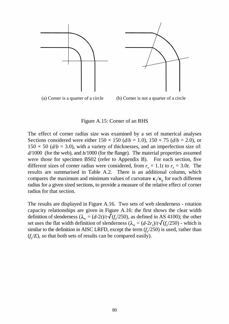
(a) Corner is a quarter of a circle (b) Corner is not a quarter of a circle

80

Figure A.15: Corner of an RHS

The effect of corner radius size was examined by a set of numerical analysesSections considered were either 150 × 150 (d/b = 1.0), 150 × 75 (d/b = 2.0), or150 × 50 (d/b = 3.0), with a variety of thicknesses, and an imperfection size of:d/1000 (for the web), and b/1000 (for the flange). The material properties assumedwere those for specimen BS02 (refer to Appendix B). For each section, fivedifferent sizes of corner radius were considered, from r = 1.1t to r = 3.0t. Thee e

results are summarised in Table A.2. There is an additional column, whichcompares the maximum and minimum values of curvature � /� for each different1 p

radius for a given sized sections, to provide a measure of the relative effect of cornerradius for that section.

The results are displayed in Figure A.16. Two sets of web slenderness - rotationcapacity relationships are given in Figure A.16: the first shows the clear widthdefinition of slenderness (� = (d-2t)/t·�(f /250), as defined in AS 4100); the otherw y

set uses the flat width definition of slenderness (� = (d-2r )/t·�(f /250) - which isw e y

similar to the definition in AISC LRFD, except the term (f /250) is used, rather thany

(f /E), so that both sets of results can be compared easily).y

(�1/�p)min

(�1/�p)max

81

Section r = 1.1t r = 1.5t r = 2.0t r = 2.5t r = 3.0te

R R R R Re e e e

150 × 50 × 2.0 0.46 0.45 0.47 0.47 0.49 1.03

150 × 50 × 2.5 1.43 1.44 1.38 1.41 1.42 1.03

150 × 50 × 3.0 2.97 2.95 2.89 2.89 2.92 1.02

150 × 50 × 3.5 5.11 5.05 4.93 4.90 4.94 1.04

150 × 50 × 4.0 7.37 7.37 7.29 7.21 7.17 1.02

150 × 50 × 4.5 9.73 9.61 9.30 9.17 8.94 1.08

150 × 90 × 2.5 0.37 0.36 0.35 0 0.30 1.22

150 × 90 × 3.0 0.97 0.97 0.98 0.97 1.01 1.02

150 × 90 × 3.5 1.93 1.97 1.99 1.97 1.81 1.06

150 × 90 × 4.0 3.16 3.19 3.17 3.17 3.23 1.02

150 × 90 × 4.5 4.67 4.83 4.79 4.84 4.96 1.05

150 × 90 × 5.0 6.61 6.64 6.33 6.58 6.73 1.05

150 × 90 × 5.5 8.64 8.58 8.55 8.58 8.61 1.01

150 × 150 × 4.0 0 0 0 0.51 0.56 1.04

150 × 150 × 4.5 1.09 1.10 1.09 1.11 1.08 1.01

150 × 150 × 5.0 1.67 1.67 1.69 1.69 1.76 1.03

150 × 150 × 5.5 2.12 2.11 2.16 2.43 2.29 1.10

150 × 150 × 6.0 3.02 2.91 2.88 2.92 3.11 1.06

150 × 150 × 7.0 4.44 4.47 4.66 4.69 4.97 1.10

150 × 150 × 8.0 7.07 7.08 7.08 7.17 7.59 1.06

Average 1.05

Standard deviation 0.048

Table A.2: Summary of Results for Different Corner Radius Size

0

2

4

6

8

10

12

10 20 30 40 50 60 70 80 90 100

Web Slenderness λw = (d -2t )/t ·√(f y/250) or (d -2r e)/t·√(f y/250)

Rot

atio

n ca

paci

ty , R

Clear width: d/b = 3.0

Flat width: d/b = 3.0





The trend lines join the values for r e = 2.0t

82

Figure A.16: Web Slenderness - Rotation Capacity Relationship for Sectionswith Varying Corner Radius

Several important observations can be made:Changing the radius size altered the rotation capacity. Hence, the clear widthdefinition of slenderness is not strictly correct, as members with the sameclear width slenderness (but different radius size) had varying rotationcapacities. However, the changes in rotation capacity for a given sectionwere generally small, with an average of 5 % variation as the radius changed.For 16 out of the 20 different RHS considered, the variation was less than orequal to 6 %.

For a given aspect ratio, the spread of results in the web slenderness -rotation capacity relationship was smaller when using the clear widthslenderness, compared to the flat width slenderness. This suggests that theclear width slenderness definition gives more precise results whenconsidering the correlation between rotation capacity and slenderness,particularly if the size of the corner radius is unknown.

Loading

Supports

RHS

L1 = 800 mm

L2 = 1700 mm

83

Most unexpectedly, for RHS with d/b = 3.0 and thicknesses t � 3.5 mm, therotation capacity increased as the flat width slenderness increased (cornerradius decreased), indicating that the flat width slenderness is inappropriatefor this case.

No definitive conclusions can be made from the small range of sections considered,but the limited results suggest that the trend between web slenderness and rotationcapacity, is more accurately defined when the clear width definition of slendernessis used, rather than the flat width definition.

A.5 EFFECT OF BEAM LENGTH

All the analyses up to this stage have used the same longitudinal dimensions, asdefined in Figure A.17. A small series of analyses was carried out to examine theeffect of changing the length, L . Two sections were considered, 100 × 50 × 2 and1

150 × 50 × 4. Sinusoidally varying imperfections were included in the flanges andwebs, and the material properties assumed were those of specimen BS02 (refer toAppendix B). Because of symmetry, the ABAQUS model only considers half thelength of the beam, so three values of L /2 were considered: L /2 = 400 mm1 1

(default), 500 mm, and 600 mm. L was increased, so that the value (L - L )2 2 1

remained constant. The different moment - curvature graphs are given inFigures A.18 and A.19, and the code in the legend refers to the RHS dimensions,and the value of L /2.1

Figure A.17: Simplified Representation the Plastic Bending Tests

0

0.2

0.4

0.6

0.8

1

1.2

1.4

0 0.5 1 1.5 2 2.5 3 3.5 4


Non

Dim

ensi

onal

Mom

ent M

/Mp

100_50_2_L_400

100_50_2_L_500

100_50_2_L_600

0

0.2

0.4

0.6

0.8

1

1.2

1.4

0 2 4 6 8 10


Non

Dim

ensi

onal

Mom

ent M

/Mp

150_50_4_L_400

150_50_4_L_500

150_50_4_L_600

84

Figure A.18: Effect of Specimen Length of 100 × 50 × 2 RHS

Figure A.19: Effect of Specimen Length of 150 × 50 × 4 RHS

85

Figures A.18 and A.19 indicate that there was no significant difference in therotation capacity as the beam length increased. The post-buckling response wasslightly different in each case, since the relative size of the buckle with respect tothe beam length changed, and the curvature was an averaged value over the beamlength (see Section 2.9.5).

It is not unexpected that the behaviour was barely affected by beam length. Onesymmetry condition imposed on the RHS was that out-of-plane deflections wereprevented, so there was no possibility of the interaction between local and flexural-torsional (lateral) buckling.

A.6 EFFECT OF WELDING

A.6.1 INTRODUCTION

In the main body of this report, geometric imperfections were imposed on the RHSbeams, and had a significant effect on the rotation capacity. The type ofimperfections imposed were bow-out imperfections, the amplitude of which variedsinusoidally along the length of the RHS beam. However, this was not the shape ofthe imperfections that were measured. The measured imperfection profiles, givenin Appendix C, showed that the bow-out imperfection was approximately constantalong the length of the beam, but there were imperfections near the loading plate,caused by the welding of the plate to the RHS, that could not be measured. It wasthought that the imperfections caused by the welding were a major factor in causinglocal buckling, and the sinusoidally varying imperfection imposed attempted tosimulate the effect of the “real” imperfections. Hence, some preliminary analyseswere performed, to investigate how the process of welding induced imperfectionsinto a specimen, and how the rotation capacity was affected. The process ofwelding was simulated by imposing a heat differential. The weld material wasassumed to be at a high temperature, and then it was cooled, which inducedimperfections and stresses into the RHS beam, prior to the bending of the beam.Various changes in temperature were considered.

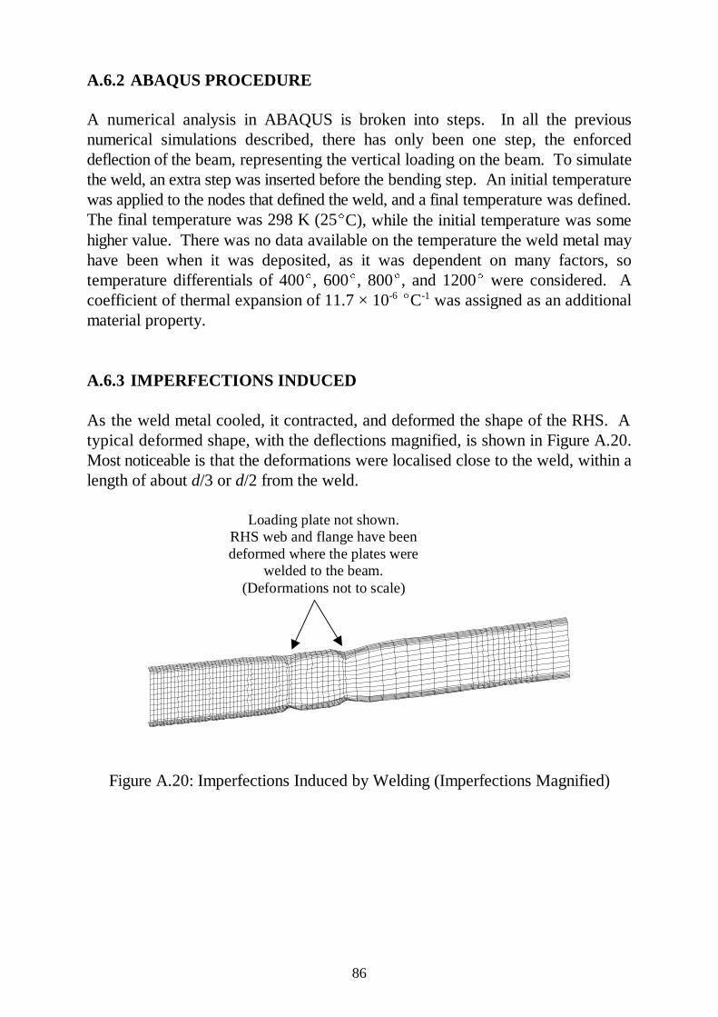
Loading plate not shown.RHS web and flange have beendeformed where the plates were

welded to the beam.(Deformations not to scale)

86

A.6.2 ABAQUS PROCEDURE

A numerical analysis in ABAQUS is broken into steps. In all the previousnumerical simulations described, there has only been one step, the enforceddeflection of the beam, representing the vertical loading on the beam. To simulatethe weld, an extra step was inserted before the bending step. An initial temperaturewas applied to the nodes that defined the weld, and a final temperature was defined.The final temperature was 298 K (25(C), while the initial temperature was somehigher value. There was no data available on the temperature the weld metal mayhave been when it was deposited, as it was dependent on many factors, sotemperature differentials of 400(, 600(, 800(, and 1200( were considered. Acoefficient of thermal expansion of 11.7 × 10 (C was assigned as an additional-6 -1

material property.

A.6.3 IMPERFECTIONS INDUCED

As the weld metal cooled, it contracted, and deformed the shape of the RHS. Atypical deformed shape, with the deflections magnified, is shown in Figure A.20.Most noticeable is that the deformations were localised close to the weld, within alength of about d/3 or d/2 from the weld.

Figure A.20: Imperfections Induced by Welding (Imperfections Magnified)

Deformed shapedue to bow-out

imperfection only(black line)

Deformed shapeafter temperature

change(grey line)

87

Figure A.20 gives a spurious impression of the nature of the imperfections inducedby welding, as the deformations caused by the cooling of the weld have beenmagnified, but the initial imperfections have not been magnified by the same factor.Figure A.21 shows the cross section of the RHS adjacent to the weld. The initialimperfection and the weld induced deformations are magnified by the same amount.The initial imperfection sizes were +d/500 and -b/500, and the temperature changewas 400(. The deformation caused by the cooling of the weld was much smallerthan the amplitude of the sinusoidally varying “bow-out” initial imperfections.

Figure A.21: Imperfections Induced by Welding(Imperfections and deformations magnified by same factor)

A.6.4 RESULTS

The results of the ABAQUS simulations are summarised in Table A.3 and themoment - curvature relationships are shown in Figure A.22. Two types ofimperfections were considered; the first where the bow-out imperfection wasconstant along the length of the beam, and the other in which the amplitude of thebow-out varied sinusoidally.

88

Section Type of Imperfection Temperature Rimperfection size difference

150 × 50 × 3.0 None 0 0(C 3.97

150 × 50 × 3.0 None 0 400(C 3.93

150 × 50 × 3.0 Constant bow-out 1/500 0(C 3.97





150 × 50 × 3.0 Sinusoidal bow-out 1/500 0(C 2.32






Experimental BS03A 2.7

Experimental BS03B 2.3

Experimental BS03C 2.9

Table A.3: Summary of Results Examining Effect of Weld Temperature

0

0.2

0.4

0.6

0.8

1

1.2

1.4

0 1 2 3 4 5 6


Non

Dim

ensi

onal

Mom

ent M

/Mp

150_50_3_bow_delt_000 150_50_3_bow_delt_400150_50_3_bow_delt_600 150_50_3_bow_delt_800150_50_3_bow_delt_1200 150_50_3_nobow_delt_000150_50_3_nobow_delt_400 150_50_3_wave_delt_000150_50_3_wave250_delt_000 150_50_3_wave_delt_400150_50_3_wave_delt_600 150_50_3_wave_delt_800150_50_3_wave_delt_1200 Experimental - BS03B

89

Figure A.22: Moment - Curvature Graphs for Imperfection Types and Weld Temperatures

A.6.5 DISCUSSION

It is clear that simulating a temperature change in the weld affects the rotationcapacity, but only slightly. For sections with the initial constant bow-outimperfection, only the largest temperature change of 1200(C made a significantimpact on rotation capacity, however the rotation capacity still exceeded theexperimentally observed value.

The introduction of sinusoidally varying imperfections had a more significant impacton rotation capacity than inclusion of temperature effects. When the temperaturechanged was enforced on a section which already had sinusoidally varyingimperfections, the effect on rotation capacity was insignificant.

An uncertainty in the analysis was the value of temperature change to be prescribed.The temperature of the weld metal is dependent on the welding procedure,consumables etc.

The conclusion to be drawn is that the amplitude of the sinusoidally varying bow-outimperfections is a critical factor in simulating the experimental results. The effectof the weld cooling slightly changes the magnitude of the initial imperfections.

90

The ABAQUS simulations described above are only preliminary, and there is largescope for further analyses to examine the effect of welding: not only howimperfections and stresses induced can affect the stability of a section, but also howthe heat affects material properties such as ductility.

A.7 CONCLUSION

This appendix considered various parameters in the finite element analysis of RHSbeams.

Different idealised material properties were considered: elastic - plastic, elastic -strain hardening, and elastic - plastic - strain hardening. The most importantobservation was that increasing strain hardening modulus increased the rotationcapacity.

Several RHS sections, which varied only by the size of the corner radius, wereanalysed, to consider whether the flat width or clear width definition of slendernesswas more appropriate to use to describe the slenderness - rotation capacityrelationship. The limited results suggest that the trend between web slenderness androtation capacity, is described better when the clear width definition of slendernessis used, rather than the flat width definition..

Some preliminary analyses were made to examine the effect of the welding of theloading plates to the RHS. The weld was initially hot, and as the weld metal cooled,it induced deformations into the RHS, but the deformations induced wereconsiderably smaller than the typical initial imperfections. The amplitude of thesinusoidally varying bow-out imperfections is a more critical factor in simulating theexperimental results.

91

Appendix B

TENSILE COUPON TESTS AND STRESS - STRAINCURVES

B.1 GENERAL

Tensile coupon tests were performed on the RHS as part of the test series on cold-formed RHS beams (Wilkinson and Hancock 1997, Wilkinson 1999). Thisappendix summarises the results of the tensile coupon tests, tabulating the yieldstress (f ) and ultimate tensile strength (f ). The stress strain curves are also given.y u

Coupons were cut from the various flat faces and corners of the RHS (refer toFigure 1).

The “engineering” stress strain curves in this appendix were converted to “true”stress and strain values, as described in Section 2.6, and subsequently used in thefinite element analyses. It was possible to prescribe different material properties tothe webs, flanges and corners of the RHS.

Details of the tensile testing procedure are available in Wilkinson and Hancock(1997) and Wilkinson (1999).

fu

fy

92

Spec- Cut from Posi- E f f e E fimen section tion (GPa) (MPa) (MPa) (%) (GPa) (MPa)

y u f1

y1

Adj 1 198 425 492 1.16 18.0TS01D 150 × 50 × 5.0 Adj 2 198 457 498 1.09 16.2 198 441

C450 Opp 213 505 543 1.07 15.6C1 200 520 556 1.07 20.02

C2 200 480 566 1.18 16.72

C3 200 495 566 1.14 16.72

C4 200 500 560 1.12 18.32

Adj 1 219 460 537 1.17 20.3TS02D 150 × 50 × 4.0 Adj 2 205 454 516 1.14 18.3 212 457

C450 Opp 198 514 580 1.13 15.7C1 200 563 616 1.09 17.22

C2 200 545 601 1.10 16.02

C3 200 550 608 1.11 16.02

C4 200 570 613 1.08 18.02

Adj 1 210 445 520 1.17 19.9TS03D 150 × 50 × 3.0 Adj 2 201 442 506 1.14 16.6 206 444

C450 Opp 218 514 585 1.14 13.2C13

C2 200 540 588 1.09 20.02

C3 200 545 594 1.09 20.02

C4 200 540 611 1.13 20.02

Adj 1 202 445 527 1.18 15.2TS04D 150 × 50 × 2.5 Adj 2 206 446 518 1.16 16.3 204 446

C450 Opp 204 485 560 1.15 13.1C1 200 540 600 1.11 25.02

C2 200 530 585 1.10 20.02

C3 200 545 596 1.09 20.02

C4 200 540 588 1.09 17.52

Adj 1 207 453 528 1.17 16.3TS05D 150 × 50 × 2.3 Adj 2 204 434 508 1.17 18.3 205 444

C450 Opp 191 480 547 1.14 14.5C1 200 535 585 1.09 17.52

C2 200 470 523 1.11 17.52

C3 200 490 526 1.07 21.02

C4 200 480 530 1.10 18.52

Adj 1 194 445 492 1.11 12.9TS06D 100 × 50 × 2.0 Adj 2 209 452 505 1.12 10.9 202 449

C450 Opp 182 480 540 1.13 9.17C1 200 490 538 1.10 17.52

C2 200 490 540 1.10 15.02

C3 200 510 560 1.10 20.02

C4 200 500 547 1.09 20.02

Table B.1: Summary of Tensile Test Results

fu

fy

93


y u f1

y1

Adj 1 199 345 430 1.25 28.3TS07D 75 × 50 × 2.0 Adj 2 208 411 484 1.18 12.5 203 4114

C450 Opp 196 428 482 1.13 23.3C1 200 475 520 1.09 18.52

C2 200 450 500 1.11 17.52

C3 200 445 480 1.08 19.02

C4 200 465 503 1.08 20.02

Adj 1 202 438 507 1.16 14.2TS08D 75 × 25 × 2.0 Adj 2 204 475 522 1.10 11.0 203 457

C450 Opp 204 487 537 1.10 26.0C1 200 480 538 1.12 19.02

C2 200 550 588 1.07 15.02

C3 200 530 576 1.09 18.52

C4 200 525 585 1.11 15.02

Adj 1 194 450 506 1.12 26.0TS09D 75 × 25 × 1.6 Adj 2 193 428 515 1.20 12.5 193 439

C450 Opp 200 487 545 1.12 14.0C1 200 560 589 1.05 16.72

C2 200 555 576 1.04 14.72

C3 200 555 605 1.09 14.72

C4 200 565 585 1.04 16.72

Adj 1 205 421 460 1.09 16.1TS10D 75 × 25 × 1.6 Adj 2 199 423 452 1.07 17.2 202 422

C350 Opp 206 445 514 1.16 6.25C1 200 505 540 1.07 16.02

C2 200 500 515 1.03 16.72

C3 200 510 532 1.04 17.32

C4 200 510 555 1.09 15.32

Adj 1 207 370 433 1.17 32.6TS11D 150 × 50 × 3.0 Adj 2 202 369 425 1.15 27.9 205 370

C350 Opp 198 380 436 1.15 22.2C1 200 465 511 1.10 20.02

C2 200 475 516 1.09 22.52

C3 200 480 534 1.11 21.02

C4 200 495 542 1.09 20.52

Adj 1 205 395 454 1.15 21.1TS12D 100 × 50 × 2.0 Adj 2 200 404 445 1.10 19.0 203 400

C350 Opp 199 433 471 1.08 12.0C1 200 500 536 1.07 21.02

C2 200 485 530 1.09 21.52

C3 200 480 520 1.08 20.02

C4 200 505 545 1.08 22.52

Table B.1 (continued): Summary of Tensile Test Results

fu

fy

94


y u f1

y1

Adj 1 211 396 450 1.14 25.0TS13D 125 × 75 × 3.0 Adj 2 210 397 448 1.13 28.4 211 397

C350 Opp 203 403 453 1.12 19.1C1 200 470 510 1.09 23.02

C2 200 475 518 1.09 22.52

C3 200 475 508 1.07 24.02

C4 200 470 520 1.11 22.52

Adj 1 204 350 436 1.25 36.3BJ07 150 × 50 × 4.0 Adj 2 204 348 438 1.26 36.3 204 349

C350 Opp 185 367 433 1.18 43.7

Adj 1 207 409 460 1.12 38.8Frame 1 150 × 50 × 4.0 Adj 2 208 412 468 1.14 35.0 207 411BF01 C350 Opp 207 425 474 1.12 27.5

C 1 201 560 590 1.05 18.3C 2 200 555 591 1.06 16.7C 3 200 565 600 1.06 13.3C 4 200 560 598 1.07 15.0

Adj 1 208 455 530 1.16 30.0Frame 2 150 × 50 × 4.0 Adj 2 205 420 510 1.21 32.9 207 437Frame 3 C450 Opp 204 455 520 1.14 48.8BF02 C 1 198 565 612 1.08 13.3

C 2 205 585 630 1.08 15.0C 3 208 585 630 1.08 15.0C 4 204 565 620 1.10 18.3

Notes: (1) The average of E and f for the two adjacent sides is used for the whole RHS.y

(2) For corner coupons it is assumed that E = 200 GPa.(3) Specimen TS03DC1 not tested.(4) For TS07D f is from face Adjacent 2 only.y

(5) Nominal strengths: Grade C450 specimens f = 450 MPa and f = 500 MPa.yn un

Grade C350 specimens f = 350 MPa and f = 430 MPa.yn un

.

. Table B.1 (continued): Summary of Tensile Test Results

Stress Strain CurveTS01D 150 x 50 x 5.0 C450

0

100

200

300

400

500

600

700

0 0.02 0.04 0.06 0.08 0.1 0.12 0.14 0.16

Strain

Str

ess

(MP

a)

Adjacent 1 Adjacent 2

Opposite Corner 1

Corner 2 Corner 3

Corner 4

Strain determinedfrom gauges

Strain determinedfrom totalextension


0

100

200

300

400

500

600

700

0 0.02 0.04 0.06 0.08 0.1 0.12 0.14 0.16 0.18

Strain

Str

ess

(MP

a)


Opposite Corner 1

Corner 2 Corner 3

Corner 4




0

100

200

300

400

500

600

700

0 0.02 0.04 0.06 0.08 0.1 0.12 0.14 0.16 0.18

Strain

Str

ess

(MP

a)

Adjacent 1

Adjacent 2

Opposite

Corner 2

Corner 3

Corner 4

Corner 1 not tested



95

Figure B.1: Stress - Strain Curve for Specimen TS01D




0

100

200

300

400

500

600

700

0 0.02 0.04 0.06 0.08 0.1 0.12 0.14

Strain

Str

ess

(MP

a)

Adjacent 1

Adjacent 2

Opposite

Corner 1

Corner 2

Corner 3

Corner 4




0

100

200

300

400

500

600

700

0 0.02 0.04 0.06 0.08 0.1 0.12 0.14 0.16

Strain

Str

ess

(MP

a)

Adjacent 1

Adjacent 2

Opposite

Corner 1

Corner 2

Corner 3

Corner 4




0

100

200

300

400

500

600

700

0 0.02 0.04 0.06 0.08 0.1 0.12

Strain

Str

ess

(MP

a)

Adjacent 1

Adjacent 2

Opposite

Corner 1

Corner 2

Corner 3

Corner 4



96





0

100

200

300

400

500

600

0 0.02 0.04 0.06 0.08 0.1 0.12 0.14 0.16

Strain

Str

ess

(MP

a)

Adjacent 1

Adjacent 2

Opposite

Corner 1

Corner 2

Corner 3

Corner 4




0

100

200

300

400

500

600

700

0 0.01 0.02 0.03 0.04 0.05 0.06 0.07 0.08 0.09 0.1

Strain

Str

ess

(MP

a)

Adjacent 1

Adjacent 2

Opposite

Corner 1

Corner 2

Corner 3

Corner 4




0

100

200

300

400

500

600

700

0 0.02 0.04 0.06 0.08 0.1 0.12

Strain

Str

ess

(MP

a)

Adjacent 1

Adjacent 2

Opposite

Corner 1

Corner 2

Corner 3

Corner 4



97





0

100

200

300

400

500

600

700

0 0.02 0.04 0.06 0.08 0.1 0.12 0.14 0.16 0.18 0.2

Strain

Str

ess

(MP

a)

Adjacent 1

Adjacent 2

Opposite

Corner 1

Corner 2

Corner 3

Corner 4




0

100

200

300

400

500

600

0 0.05 0.1 0.15 0.2 0.25 0.3

Strain

Str

ess

(MP

a)

Adjacent 1

Adjacent 2

Opposite

Corner 1

Corner 2

Corner 3

Corner 4




0

100

200

300

400

500

600

0 0.02 0.04 0.06 0.08 0.1 0.12 0.14 0.16 0.18 0.2

Strain

Str

ess

(MP

a)

Adjacent 1

Adjacent 2

Opposite

Corner 1

Corner 2

Corner 3

Corner 4



98





0

100

200

300

400

500

600

0 0.05 0.1 0.15 0.2 0.25

Strain

Str

ess

(MP

a)

Adjacent 1

Adjacent 2

Opposite

Corner 1

Corner 2

Corner 3

Corner 4



Stress Strain CurveKJ07, KJ08, KJ12, SJ03 150 x 50 x 4.0 C350

0

50

100

150

200

250

300

350

400

450

500

0 0.05 0.1 0.15 0.2 0.25 0.3

Strain

Str

ess

(MP

a)

Adjacent 1

Adjacent 2

Opposite



Stress Strain CurveFrame 1 150 x 50 x 4.0 C350

0

100

200

300

400

500

600

700

0 0.05 0.1 0.15 0.2 0.25

Strain

Str

ess

(MP

a)


Opposite Corner 1

Corner 2 Corner 3

Corner 4

99


Figure B.14: Stress - Strain Curve for Specimen KJ07

Figure B.15: Stress - Strain Curve for Frame 1

Stress Strain CurveFrame 2 & Frame 3 150 x 50 x 4.0 C450

0

100

200

300

400

500

600

700

0 0.05 0.1 0.15 0.2 0.25 0.3

Strain

Str

ess

(MP

a)


Opposite Corner 1

Corner 2 Corner 3

Corner 4

100

Figure B.16: Stress - Strain Curve for Frames 2 and 3

101

Appendix C

IMPERFECTION MEASUREMENTS

C.1 INTRODUCTION

RHS are not perfect rectangular specimens. The cold-forming process, welding,handling and other factors can introduce geometric imperfections. Localimperfections can have a significant effect on the moment and rotation capacity(Key and Hancock 1993). Hence the local imperfections of the RHS were measuredas part of the test program. The nature of the imperfection is important insubsequent finite element modelling of the bending tests.

C.2 METHOD

The method of measuring the geometric imperfections is described in Wilkinson andHancock (1997) and Wilkinson (1999).

C.3 RESULTS

Most RHS exhibited a “bow-out” (as shown in Figure C.1) or “bow-in” on each flatface of the section that was reasonably constant along the length of the RHS. It wasmost common for there to be a bow-out on each web, and a bow-in on each flange.The magnitude of the imperfection was approximately constant along the length ofthe specimen, that is, no significant wave-like imperfections along the length weredetected. It was not possible to measure imperfections close to the loading platesthat were welded to the specimen (refer to Figure 4). Visible inspection of thespecimens indicated that there was some imperfection induced into the specimennext to the welds connecting the loading plates to the RHS.

The profiles are shown in Figure C.3 to C.26. It can be observed that the values ofthe imperfections are small (typically less than ± 1% of the specimen dimension).The stiffer faces of the RHS tend to exhibit a negative imperfection (an inwardsbow), while the other faces exhibit an outwards bow. For example a “thick”specimen, BS01C, exhibits inwards imperfection on all faces, and a thinnerspecimen exhibits bow-out on the less stiff webs but inwards bowing on the stifferflanges.

δ

102

Figure C.1: Typical “Bow-Out” Imperfection of an RHS (note: bow-out exaggerated)

The imperfection resulted from the cold-forming process. The coil of steel wasinitially rolled as a circle and then the centre of each face was pushed in bysuccessive sets of rollers to form the rectangular shape. The same set of rollers wasused for the same outer size of RHS and hence similar force formed the section intothe rectangular shape. The thinner sections tend to “spring back” more after passinga set of rolls causing the “bow-out”.

This imperfection was generally approximately constant along the length of thebeam. There was often some extra initial deformation near the loading plates,caused by welding of the loading plates and the clamping of the samples during thiswelding, but it was difficult to measure such imperfections accurately. There wasmore variability in the profile of the smaller specimens - it was more difficult tomeasure these samples accurately, and smaller values of these imperfectionsapproach the precision of the displacement transducer. The profile of the weld faceof the RHS was often difficult to measure precisely due to the seam of the join onthe outside of the RHS.

The figures give the “bow-out” deformation along the length of the RHS specimenat six positions along the flange and web shown below.

δ6

δ5

δ4

δ3

δ2

δ1

Opp

Weld

Adj 1Adj 2

103

Figure C.2: Location of Imperfection Profile Measurement

Section ProfileBS01C 150 x 50 x 5.0 C450

-0.8

-0.7

-0.6

-0.5

-0.4

-0.3

-0.2

-0.1

0

100 200 300 400 500 600 700 800

Distance Along Specimen between Loading Points (mm)

"Bow

Out

" Im

perf

ectio

n (m

m)

Position 1

Position 2

Position 3

Position 4

Position 5

Position 6

Section ProfileBS02A 150 x 50 x 4.0 C450

-0.4

-0.35

-0.3

-0.25

-0.2

-0.15

-0.1

-0.05

0

100 200 300 400 500 600 700 800


"Bow

Out

" Im

perf

ectio

n (m

m)

Position 1

Position 2

Position 3

Position 4

Position 5

Position 6


-0.45

-0.4

-0.35

-0.3

-0.25

-0.2

-0.15

-0.1

-0.05

0

100 200 300 400 500 600 700 800


"Bow

Out

" Im

perf

ectio

n (m

m)

Position 1

Position 2

Position 3

Position 4

Position 5

Position 6

104

Figure C.3: Section Profile for BS01C

Figure C.4: Section Profile for BS02A



-0.3

-0.2

-0.1

0

0.1

0.2

0.3

0.4

0.5

0.6

100 200 300 400 500 600 700 800


"Bow

Out

" Im

perf

ectio

n (m

m)

Position 1

Position 2

Position 3

Position 4

Position 5

Position 6


-0.2

-0.1

0

0.1

0.2

0.3

0.4

0.5

100 200 300 400 500 600 700 800


"Bow

Out

" Im

perf

ectio

n (m

m)

Position 1

Position 2

Position 3

Position 4

Position 5

Position 6


-0.2

-0.15

-0.1

-0.05

0

0.05

0.1

0.15

0.2

0.25

0.3

0.35

100 200 300 400 500 600 700 800


"Bow

Out

" Im

perf

ectio

n (m

m)

Position 1

Position 2

Position 3

Position 4

Position 5

Position 6

105





-0.2

-0.1

0

0.1

0.2

0.3

0.4

0.5

0.6

0.7

100 200 300 400 500 600 700 800


"Bow

Out

" Im

perf

ectio

n (m

m)

Position 1

Position 2

Position 3

Position 4

Position 5

Position 6


-0.2

-0.1

0

0.1

0.2

0.3

0.4

0.5

0.6

0.7

0.8

0.9

100 200 300 400 500 600 700 800


"Bow

Out

" Im

perf

ectio

n (m

m)

Position 1

Position 2

Position 3

Position 4

Position 5

Position 6


-0.6

-0.4

-0.2

0

0.2

0.4

0.6

100 200 300 400 500 600 700 800


"Bow

Out

" Im

perf

ectio

n (m

m)

Position 1

Position 2

Position 3

Position 4

Position 5

Position 6

106




Section ProfileBS07B 75 x 50 x 2.0 C450

-0.15

-0.1

-0.05

0

0.05

0.1

0.15

0.2

0.25

0.3

100 150 200 250 300 350 400 450


"Bow

Out

" Im

perf

ectio

n (m

m)

Position 1

Position 2

Position 3

Position 4

Position 5

Position 6


-0.05

0

0.05

0.1

0.15

0.2

0.25

0.3

0.35

0.4

0.45

0.5

100 150 200 250 300 350 400 450


"Bow

Out

" Im

perf

ectio

n (m

m)

Position 1

Position 2

Position 3

Position 4

Position 5

Position 6


-0.3

-0.2

-0.1

0

0.1

0.2

0.3

0.4

100 150 200 250 300 350 400 450


"Bow

Out

" Im

perf

ectio

n (m

m)

Position 1

Position 2

Position 3

Position 4

Position 5

Position 6

107

Figure C.12: Section Profile for BS07B




-0.3

-0.2

-0.1

0

0.1

0.2

0.3

0.4

100 150 200 250 300 350 400 450


"Bow

Out

" Im

perf

ectio

n (m

m)

Position 1

Position 2

Position 3

Position 4

Position 5

Position 6


-0.1

0

0.1

0.2

0.3

0.4

0.5

0.6

100 150 200 250 300 350 400 450


"Bow

Out

" Im

perf

ectio

n (m

m)

Position 1

Position 2

Position 3

Position 4

Position 5

Position 6


-0.1

0

0.1

0.2

0.3

0.4

0.5

0.6

100 150 200 250 300 350 400 450


"Bow

Out

" Im

perf

ectio

n (m

m)

Position 1

Position 2

Position 3

Position 4

Position 5

Position 6

108





-0.2

-0.1

0

0.1

0.2

0.3

0.4

0.5

100 150 200 250 300 350 400 450


"Bow

Out

" Im

perf

ectio

n (m

m)

Position 1

Position 2

Position 3

Position 4

Position 5

Position 6


-0.1

0

0.1

0.2

0.3

0.4

0.5

100 150 200 250 300 350 400 450


"Bow

Out

" Im

perf

ectio

n (m

m)

Position 1

Position 2

Position 3

Position 4

Position 5

Position 6


-0.4

-0.3

-0.2

-0.1

0

0.1

0.2

0.3

0.4

0.5

0.6

0.7

100 200 300 400 500 600 700 800


"Bow

Out

" Im

perf

ectio

n (m

m)

Position 1

Position 2

Position 3

Position 4

Position 5

Position 6

109





-0.4

-0.3

-0.2

-0.1

0

0.1

0.2

0.3

0.4

0.5

0.6

100 200 300 400 500 600 700 800


"Bow

Out

" Im

perf

ectio

n (m

m)

Position 1

Position 2

Position 3

Position 4

Position 5

Position 6


-0.6

-0.4

-0.2

0

0.2

0.4

0.6

0.8

1

100 200 300 400 500 600 700 800


"Bow

Out

" Im

perf

ectio

n (m

m)

Position 1

Position 2

Position 3

Position 4

Position 5

Position 6


-0.6

-0.4

-0.2

0

0.2

0.4

0.6

0.8

1

1.2

100 200 300 400 500 600 700 800


"Bow

Out

" Im

perf

ectio

n (m

m)

Position 1

Position 2

Position 3

Position 4

Position 5

Position 6

110





-0.6

-0.4

-0.2

0

0.2

0.4

0.6

100 200 300 400 500 600 700 800


"Bow

Out

" Im

perf

ectio

n (m

m)

Position 1

Position 2

Position 3

Position 4

Position 5

Position 6


-0.2

-0.1

0

0.1

0.2

0.3

0.4

0.5

100 200 300 400 500 600 700 800


"Bow

Out

" Im

perf

ectio

n (m

m)

Position 1

Position 2

Position 3

Position 4

Position 5

Position 6


-0.3

-0.2

-0.1

0

0.1

0.2

0.3

0.4

100 200 300 400 500 600 700 800


"Bow

Out

" Im

perf

ectio

n (m

m)

Position 1

Position 2

Position 3

Position 4

Position 5

Position 6

111




112

Please visit the Department of Civil Engineering Web Sitehttp://www.civil.usyd.edu.au

R792 Finite Element Analysis of Plastic Bending of Cold ...

Documents

Transcript of R792 Finite Element Analysis of Plastic Bending of Cold ...