R2-D.2: Optimization of Explosives Sensor

Placement in Airports

I. PARTICIPANTS

Faculty/Staff

Name Title Institution Email

Qingyan “Yan” Chen PI Purdue University yanchen@purdue.edu

Graduate, Undergraduate and REU Students

Name Degree Pursued Institution Month/Year of Graduation

Wei Liu PhD Purdue University 12/2017

II. PROJECT DESCRIPTION

Core funding for this project ends in Year 3 per the outcome of the Biennial Review process. Wei Lu, the PhD student working on this project, will be supported via ALERT core funds so as to not impact his degree com-pletion. Results of the student work will be reported in a special section of the ALERT Year 4 Annual Report.

A. Project Overview

Effective detection of explosives-related threats is very important to the country and the world. In the past, the explosives detection community has invested heavily in contact sensing for portal screening. However, they are unable to answer the question: “Great sensors, but how do you know the vapors/particles get there?” This is because an airport is a large space, so the concentration of the vapors/particles of explosives are gen-erally low. It is dif icult to direct the low concentration of explosives agents to the limited amount of sensors. Therefore, our ALERT Phase 2 Year 2 project investigated how explosives vapors/particles were transported at the Indianapolis International Airport terminal; identi ied strategies that can be used to increase explo-sive vapor concentrations; and demonstrated how to use these strategies to detect explosives with suitable sensors. Computational luid dynamics (CFD) simulations were used for predictions of air distribution and contaminant transport because they are more accurate than other numerical tools, and much faster than experimental measurements. Since this application is for airports, the space is much larger than those in the previous studies. Thus, CFD was found to be very expensive when it is used to ind optimal sensor locations and to identify source positions. Therefore, our ALERT Phase 2 Year 3 project developed and validated the fast luid dynamics (FFD), which was a faster method than CFD while maintaining the accuracy. The research can provide effective methods to detect explosives vapors in airports.

B. Biennial Review Results and Related Actions to Address

This project was slated for sunset in the last Biennial Review and was concluded at the end of Year 3. Through discussion following the Biennial Review process, the ALERT Director allocated ALERT core funding to be used in Year 4 to support Wei Lu, a Ph.D. candidate working on this project.The major strength of this project is that the developed FFD solvers can be almost 40 times faster than CFD in predicting transient low. The major weakness is that the developed FFD solvers do not have the user interface. It requires a lot coding to use it, which limits its application in the engineering ield. Therefore, our

ALERT Phase 2 Year 3 Annual Report

Appendix A: Project Reports Thrust R2: Trace & Vapor Sensors

Project R2-D.2

Year 4 project plans to develop the user interface for the FFD solvers. The work will be done by Mr. Liu as part of his Ph.D. requirement.

C. State of the Art and Technical Approach

Optimal sensor placement in an enclosed space requires predictions on air distribution and contaminant transport. As summarized by Chen [1], the numerical tools include nodal models (multi-zone model and zonal model) and CFD simulation. The nodal models can be very fast, but they only provide averaged charac-teristics of air lows and contaminant distributions within particular zones [2]. Signi icant errors may arise in large indoor spaces with strati ied ventilation systems or strong jet momentums [3, 4]. Thus, the accuracy of a nodal model depends on the user’s ability to identify different low characteristics in different regions. CFD simulation provides the most detailed information about distributions of air velocity, temperature, contami-nant dispersion, etc. When it is used for indoor air low simulations, CFD is also the most accurate approach, as it involves the fewest assumptions. CFD simulation is therefore the most popular method used today in practice [1]. However, this method requires a powerful computer in order to handle a large number of grids for a large or complex indoor space, and the computing time can be very long [5]. A faster method is desired that can provide the same detailed indoor air low information as CFD, and the same ef iciency as the nodal models.FFD, which solves the Navier-Stokes equations with a projection method, seems to meet the above require-ments. FFD has been widely applied to weather prediction and the study of atmospheric lows [6, 7, 8, 9]. Since the major development by Stam [10] in the area of computer games, FFD has been used for low sim-ulations. Zuo and Chen [11] applied FFD to fast two-dimensional (2D) air low simulations in an indoor en-vironment and found that FFD can offer much more detailed low information than do nodal models, with faster-than-real-time simulation speeds. Zuo et al. [12, 13] further improved the accuracy of FFD simulations by using the inite volume method, mass conservation correction, and a hybrid interpolation scheme. Re-cently, Jin et al. [14, 15, 16] extended FFD to the solution of three-dimensional (3D) air low and proposed a conservative SL scheme to ensure the conservation of energy and species concentration. Those efforts have made FFD simulations of indoor air low a viable alternative to CFD simulations, achieving similar accuracy with low computing time and computational capacity.Nevertheless, there are some limitations associated with using FFD for indoor air low simulations. The FFD solver developed by Zuo et al. [11] and Jin et al. [14] is applicable only to a hexahedral mesh, which cannot provide a suf iciently accurate depiction of a complex geometry such as the occupants of an indoor space. Besides, the current FFD solvers applied a semi-Lagrangian scheme to solve the advection term that would bring in signi icant numerical diffusion. The advantage is that the numerical diffusion could be used as the substitution of turbulent diffusion, so no extra turbulence model is needed. However, the signi icance of the numerical diffusion is determined by the mesh size and time step size. These two parameters are hard to determine so that the correct predictions could be obtained. Therefore, it is essential to develop FFD further for unstructured meshes that can be used to describe complex geometry and add turbulence models to FFD models without a semi-Lagrangian scheme to make it more stable and accurate. This report shows our effort in implementing FFD models in OpenFOAM (Open Field Operation and Manipulation) [17], an open-source CFD program with the capacity to handle a variety of unstructured meshes. To ensure the validity and accura-cy of our implementation, this report also describes the validation of FFD simulation for predicting different indoor air low with experimental air distribution data from the literature.

D. Major Contributions

This section discusses the fundamentals of FFD and provides the corresponding validations.

ALERT Phase 2 Year 3 Annual Report

Appendix A: Project Reports Thrust R2: Trace & Vapor Sensors

Project R2-D.2

D.1. Fast luid dynamicsFFD solves the Navier-Stokes equations in a similar manner to CFD. For incompressible viscous low in an indoor environment, the Navier-Stokes equations are:

where i, j = 1, 2, and 3. The variable Ui is the ith component of the velocity vector, p is pressure, ρ is density, Fi is the ith component of the body forces, and ν is kinetic viscosity. The previous studies used the non-incremental pressure-correction scheme with semi-Lagrangian (NIPC-SL) scheme to solve the above Navier-Stokes equa-tions. This project implemented this scheme and another three pressure-correction schemes: non-incremen-tal pressure-correction (NIPC) scheme, standard incremental pressure-correction (SIPC) scheme, and rota-tional incremental pressure-correction (RIPC) scheme in OpenFOAM.Non-incremental pressure-correction scheme The NIPC scheme is the simplest pressure-correction scheme that was originally proposed by Chorin [18] and Temam [19]. It applies a two-step time-advancement scheme that splits the momentum equation (Eq. (2)) into two discretized equations:

where Un and Un+1 represent the velocity at the previous and current time step, respectively. U* is intermediate velocities. To resolve the coupled pressure and velocity, the method uses the pressure projection [20], which substitutes Eq. (4) into Eq. (1) to produce:

The NIPC scheme irst solves Eq. (3) with the implicit Euler scheme for the temporal term; semi-implicit scheme for convection term; and implicit scheme for the diffusion term to obtain intermediate velocity U*. Then the NIPC scheme solves the Poisson equation, Eq. (5), to obtain the pressure p. Finally, the NIPC scheme calculates the velocity at the next step Un+1 by solving Eq. (4). In OpenFOAM, the solution of Eqs. (3) and (5) is straightforward.Standard incremental pressure-correction schemeAs observed by Goda [21], the pressure term is missing in Eq. (3) and adding the pressure gradient of the previous step would increase the accuracy. Then the two discretized equations are:

(1)

(2)

(3)

(4)

(5)

(6)

(7)

ALERT Phase 2 Year 3 Annual Report

Appendix A: Project Reports Thrust R2: Trace & Vapor Sensors

Project R2-D.2

where pn and pn+1 represent the pressure at the previous and current time step, respectively. U* is intermedi-ate velocities. Using the pressure projection again, we have:

Like the NIPC scheme, the SIPC scheme irst solves Eq. (6) with the implicit Euler scheme for the temporal term; semi-implicit scheme for convection term; and implicit scheme for the diffusion teem to obtain inter-mediate velocity U*. Then the SIPC scheme solves the Poisson equation, Eq. (8), to obtain the pressure pn+1. Finally, the SIPC scheme calculates the velocity at the next step Un+1 by solving Eq. (7) that is:

Rotational incremental pressure-correction scheme The NIPC scheme uses a non-physical Neumann boundary condition enforced on the pressure that is used on the numerical boundary layer. This consequently limits the accuracy of the scheme [22, 23], and will slightly modify Eq. (9) as:

The solving procedure is exactly the same with the SIPC scheme.Non-incremental pressure-correction scheme with semi-Lagrangian schemeThe NIPC-SL scheme applies a three-step time-advancement scheme [24] that splits the momentum equation (Eq. (2)) into three discretized equations:

where Un and Un+1 represent the velocity at the previous and current time step, respectively. U* and U** are intermediate velocities. Using the pressure projection, we have:

The NIPC-SL scheme irst solves Eq. (12) with the SL scheme to obtain intermediate velocity U*. Then it solves the two Poisson equations, Eqs. (13) and (15), in sequence to obtain intermediate velocity U** and pres-sure p, respectively. Finally, the algorithm calculates the velocity at the next step Un+1 by solving Eq. (14). In

(9)

(10)

(11)

(12)

(13)

(14)

(15)

(8)

ALERT Phase 2 Year 3 Annual Report

Appendix A: Project Reports Thrust R2: Trace & Vapor Sensors

Project R2-D.2

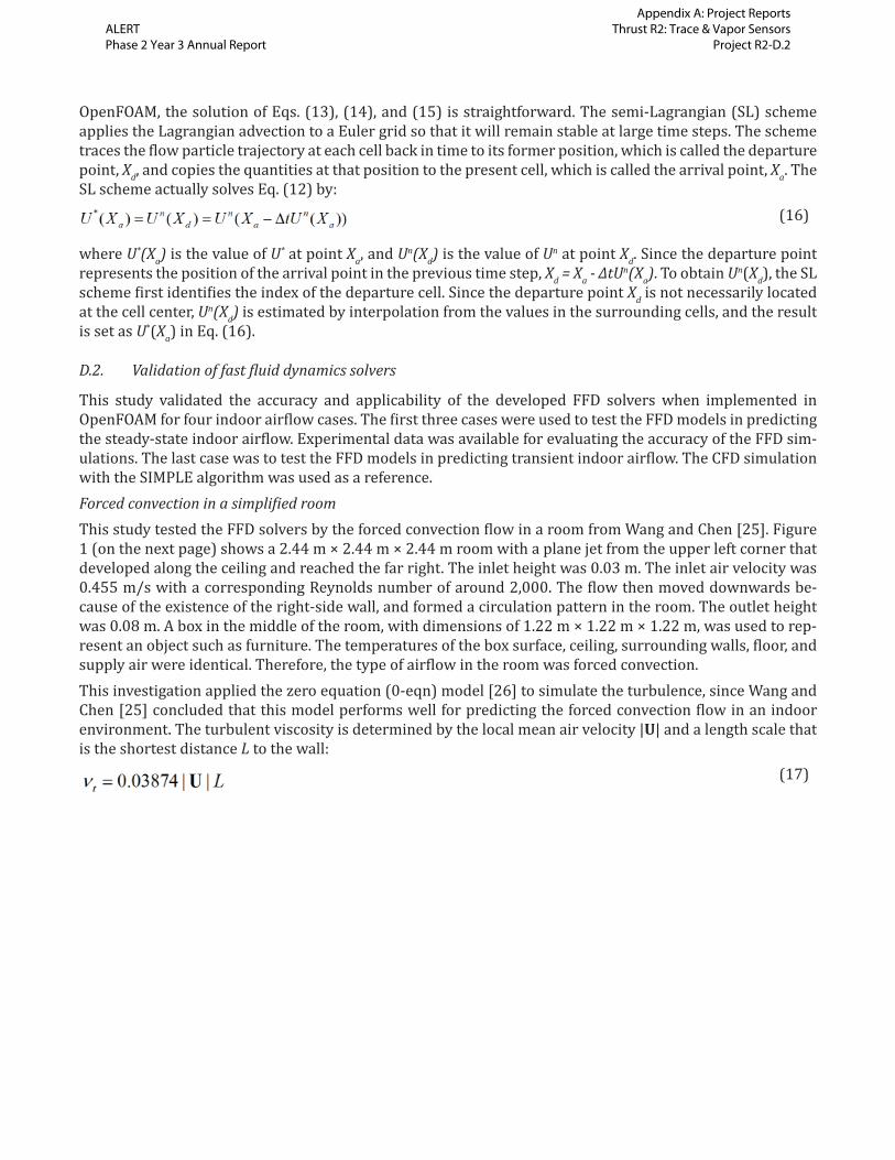
OpenFOAM, the solution of Eqs. (13), (14), and (15) is straightforward. The semi-Lagrangian (SL) scheme applies the Lagrangian advection to a Euler grid so that it will remain stable at large time steps. The scheme traces the low particle trajectory at each cell back in time to its former position, which is called the departure point, Xd, and copies the quantities at that position to the present cell, which is called the arrival point, Xa. The SL scheme actually solves Eq. (12) by: where U*(Xa) is the value of U* at point Xa, and Un(Xd) is the value of Un at point Xd. Since the departure point represents the position of the arrival point in the previous time step, Xd = Xa - ΔtUn(Xa). To obtain Un(Xd), the SL scheme irst identi ies the index of the departure cell. Since the departure point Xd is not necessarily located at the cell center, Un(Xd) is estimated by interpolation from the values in the surrounding cells, and the result is set as U*(Xa) in Eq. (16).

D.2. Validation of fast luid dynamics solvers

This study validated the accuracy and applicability of the developed FFD solvers when implemented in OpenFOAM for four indoor air low cases. The irst three cases were used to test the FFD models in predicting the steady-state indoor air low. Experimental data was available for evaluating the accuracy of the FFD sim-ulations. The last case was to test the FFD models in predicting transient indoor air low. The CFD simulation with the SIMPLE algorithm was used as a reference.Forced convection in a simpli ied roomThis study tested the FFD solvers by the forced convection low in a room from Wang and Chen [25]. Figure 1 (on the next page) shows a 2.44 m × 2.44 m × 2.44 m room with a plane jet from the upper left corner that developed along the ceiling and reached the far right. The inlet height was 0.03 m. The inlet air velocity was 0.455 m/s with a corresponding Reynolds number of around 2,000. The low then moved downwards be-cause of the existence of the right-side wall, and formed a circulation pattern in the room. The outlet height was 0.08 m. A box in the middle of the room, with dimensions of 1.22 m × 1.22 m × 1.22 m, was used to rep-resent an object such as furniture. The temperatures of the box surface, ceiling, surrounding walls, loor, and supply air were identical. Therefore, the type of air low in the room was forced convection.This investigation applied the zero equation (0-eqn) model [26] to simulate the turbulence, since Wang and Chen [25] concluded that this model performs well for predicting the forced convection low in an indoor environment. The turbulent viscosity is determined by the local mean air velocity |U| and a length scale that is the shortest distance L to the wall:

(16)

(17)

ALERT Phase 2 Year 3 Annual Report

Appendix A: Project Reports Thrust R2: Trace & Vapor Sensors

Project R2-D.2

This study compared the simulated and measured velocity distributions in Figure 2 to assess the perfor-mance of FFD solvers. The CFD simulation used the SIMPLE algorithm and the 0-eqn model was also pro-vided as a reference. In general, the velocity distributions, except the one predicted by NIPC-SL, were very similar to the measured ones. This is because the SL scheme added signi icant extra numerical diffusion.

Figure 1: Sketch of the room with a box.

Figure 2: Airfl ow patterns (arrows) measured by Wang and Chen [25] and predicted by CFD and FFD with the 0-eqn

model.

ALERT Phase 2 Year 3 Annual Report

Appendix A: Project Reports Thrust R2: Trace & Vapor Sensors

Project R2-D.2

However, it is dif icult to make quantitative comparison in Figure 2. This study thus compared the calculated air velocity pro iles with the measured data at four representative positions in the room, as shown in Figure 3 (on the next page). These positions are at the jet upstream, jet downstream, center of the room, and a location close to the side wall. The air velocity was normalized by Umax = 1.5 m/s. The CFD simulation used the SIMPLE algorithm and the 0-eq model to provide a fairly good prediction on the air velocity. The NIPC, SIPC, and RIPC with 0-eqn model had very similar performance, and the predicted air velocity pro iles agree well with the experimental data. At position 1, we can notice an obvious difference between the predicted and measured air velocity, since the air velocity there was very small. With the added numerical diffusion, the NIPC-SL with 0-eqn model had the worst performance, as it under predicted the jet low and re-circulated low.

Mixed convection in a simpli ied roomBased on the case setup in Figure 1, this case added 700 W of heat inside of the box. All other experimental conditions were exactly the same as those for the abovementioned case. The supply air temperature was con-trolled at 22.2oC. The temperatures of the box surface, ceiling, surrounding walls, and loor were 36.7, 25.8, 27.4, and 26.9oC, respectively. The heated box could form a thermal plume. Therefore, the type of air low in the room was mixed convection. This investigation again applied the 0-eqn model to simulate the turbulence, since Zhang et al. [27] concluded that this model performs well for predicting the mixed convection low in an indoor environment.This study compared the simulated and measured velocity distributions in Figure 4 (on the next page). Again, the velocity distributions, except the one predicted by NIPC-SL, were very similar to the measured ones in general. This is because the SL scheme added signi icant extra numerical diffusion. To make quantitative comparison, this study compared the calculated air velocity pro iles with the measured data at four repre-sentative positions in the room, as shown in Figure 5 (on the next page). The NIPC-SL with the 0-eqn model still performs poorly, as it under predicted the jet low and re-circulated low. The other schemes had similar performance and the predicted air velocity pro iles with the 0-eqn model agreed well with the experimental data. This con irms the performance of FFD solvers. However, there is still signi icant difference at the lower part of position 5. This is because the low there was very complicated, since the box and the jet interacted and generated a secondary recirculation. Wang and Chen [25] had tried more sophisticated models such as the Large Eddy Simulation, but it could not predict the measured velocity pro ile at this location either.

Figure 3: Comparison of air velocity profi les predicted by CFD and FFD with the 0-eqn model and the experimental

data from Wang and Chen [25] at position 1, position 3, position 5, and position 6.

ALERT Phase 2 Year 3 Annual Report

Appendix A: Project Reports Thrust R2: Trace & Vapor Sensors

Project R2-D.2

This case was non-isothermal and Figure 6 (on the next page) compares the predicted temperature pro iles with the experimental data in the same positions as shown in Figure 5. The temperature was normalized by using Tmin = 22.2oC and Tmax = 36.7oC, which were the minimum and maximum temperatures, respectively, that were observed in this case. All the numerical simulations of air temperature agreed well with the exper-imental data.

Figure 4: Airfl ow patterns (arrows) measured by Wang and Chen [25] and predicted by CFD and FFD with the 0-eqn

model.

Figure 5: Comparison of air velocity profi les predicted by CFD and FFD with the 0-eqn model and the experimental

data from Wang and Chen [25] at position 1, position 3, position 5, and position 6.

ALERT Phase 2 Year 3 Annual Report

Appendix A: Project Reports Thrust R2: Trace & Vapor Sensors

Project R2-D.2

Displacement ventilation in an of iceFigure 7 shows an occupied of ice with displacement ventilation [28]. The of ice was simulated by an exper-imental chamber of 5.16 m × 3.65 m × 2.43 m with a displacement diffuser on the side wall supplying air at a ventilation rate of 4 air changes per hour. The supply air temperature was 17oC. There are two occupants, two computers, two tables, two boxes, and six lamps in the room as shown in Figure 7(a). For detailed sizes, locations, and heat release of these items and other thermos- luid boundary conditions, one can refer to Yuan et al. [28]. The experiment measured the air temperature and air velocity along nine vertical poles distribut-ed in the stream-wise center plane and the cross-sectional center plane as shown in Figure 7(b). Figure 7(b) also shows the mesh used based on our grid independence test.

Figure 6: Comparison of air temperature profi les predicted by CFD and FFD with the 0-eqn model and the experimen-

tal data from Wang and Chen [25] at position 1, position 3, position 5, and position 6.

(a) (b)

Figure 7: (a) Schematic and (b) mesh of displacement ventilation on an occupied offi ce. The red vertical poles represent

measurement locations for air velocity and temperature.

ALERT Phase 2 Year 3 Annual Report

Appendix A: Project Reports Thrust R2: Trace & Vapor Sensors

Project R2-D.2

Since this is a much more close-to-real case, this study applied the RNG k-ε model to simulate the turbulence. Due to the poor performance of NIPC-SL in the previous two cases, this study did not consider this numerical scheme for this case. The CFD simulation used SIMPLE algorithm was again provided as a reference.This study compared the calculated air velocity pro iles with the measured data at the nine positions in the room, as shown in Figure 8. The air velocity was normalized by the inlet air velocity Uin = 0.09 m/s. The quan-titative agreement between the predicted and measured air velocity is good. All the projection methods had almost the same performance and it is hard to determine if the SIMPLE algorithm or projection methods have better performance. Figure 9 further compared the calculated air temperature pro iles with the measured data at the nine positions in the room. The normalized air temperature θ was de ined as (T – Ts)/(Tr – Ts), where Ts (supply air temperature) = 17.0oC and Tr (return air temperature) = 26.7oC. Again, the quantitative agreement between the predicted and measured air temperature is good. It implies that the projection meth-ods without SL scheme has no worse performance than the SIMPLE algorithm in predicting steady-state low in indoor environment.

Figure 8: Comparison of air velocity profi les predicted by CFD and FFD with the RNG k-ε model and the experimental

data from Yuan et al. [28]

ALERT Phase 2 Year 3 Annual Report

Appendix A: Project Reports Thrust R2: Trace & Vapor Sensors

Project R2-D.2

Mixed convection in a 2D cavityThe last case this study used was to validate the performance of projection methods in predicting transient low in an indoor environment. It was a two-dimensional, non-isothermal case with experimental data [29].

In Figure 10 (on the next page), the dimensions of the low domain were H × H = 1.04 m × 1.04 m; the inlet height was hin = 18 mm; and the outlet height was hout = 24 mm. In the experiment, the inlet air velocity was Ux = 0.57 m/s, Uy = 0.0 m/s, and the inlet air temperature (Tin) was 15oC. The temperature of the walls (Twl) was 15oC, and that of the loor (T l) was 35.5oC to form a thermal plume. The case used here is representative of air lows in enclosed environments as it includes major low characteristics in an indoor environment, such as jets and thermal plumes. Furthermore, it was not desirable to use very complex cases for this investigation since those cases may have uncertainties. Instead, this simple two-dimensional case, but still with complex low features, was more desirable for validation. Since the experiment did not measure the transient low ields, this study used the predicted air low by CFD simulation with the SIMPLE algorithm as a reference.

To eliminate the possible error brought by turbulence models, this study adopted the RNG k-ε model that is much more sophisticated than the 0-eqn model to simulate the turbulence.

Figure 9: Comparison of air temperature profi les predicted by CFD and FFD with the RNG k-ε model and the experimen-

tal data from Yuan et al [28].

ALERT Phase 2 Year 3 Annual Report

Appendix A: Project Reports Thrust R2: Trace & Vapor Sensors

Project R2-D.2

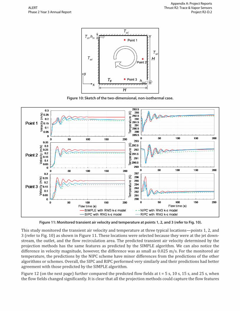
This study monitored the transient air velocity and temperature at three typical locations—points 1, 2, and 3 (refer to Fig. 10) as shown in Figure 11. These locations were selected because they were at the jet down-stream, the outlet, and the low recirculation area. The predicted transient air velocity determined by the projection methods has the same features as predicted by the SIMPLE algorithm. We can also notice the difference in velocity magnitude, however, the difference was as small as 0.025 m/s. For the monitored air temperature, the predictions by the NIPC scheme have minor differences from the predictions of the other algorithms or schemes. Overall, the SIPC and RIPC performed very similarly and their predictions had better agreement with those predicted by the SIMPLE algorithm.Figure 12 (on the next page) further compared the predicted low ields at t = 5 s, 10 s, 15 s, and 25 s, when the low ields changed signi icantly. It is clear that all the projection methods could capture the low features

Figure 10: Sketch of the two-dimensional, non-isothermal case.

Figure 11: Monitored transient air velocity and temperature at points 1, 2, and 3 (refer to Fig. 10).

ALERT Phase 2 Year 3 Annual Report

Appendix A: Project Reports Thrust R2: Trace & Vapor Sensors

Project R2-D.2

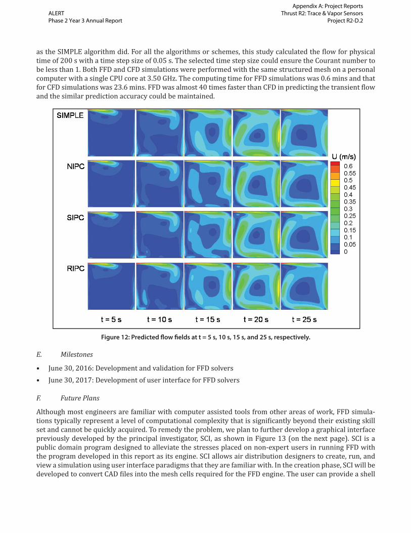
as the SIMPLE algorithm did. For all the algorithms or schemes, this study calculated the low for physical time of 200 s with a time step size of 0.05 s. The selected time step size could ensure the Courant number to be less than 1. Both FFD and CFD simulations were performed with the same structured mesh on a personal computer with a single CPU core at 3.50 GHz. The computing time for FFD simulations was 0.6 mins and that for CFD simulations was 23.6 mins. FFD was almost 40 times faster than CFD in predicting the transient low and the similar prediction accuracy could be maintained.

E. Milestones

• June 30, 2016: Development and validation for FFD solvers• June 30, 2017: Development of user interface for FFD solvers

F. Future Plans

Although most engineers are familiar with computer assisted tools from other areas of work, FFD simula-tions typically represent a level of computational complexity that is signi icantly beyond their existing skill set and cannot be quickly acquired. To remedy the problem, we plan to further develop a graphical interface previously developed by the principal investigator, SCI, as shown in Figure 13 (on the next page). SCI is a public domain program designed to alleviate the stresses placed on non-expert users in running FFD with the program developed in this report as its engine. SCI allows air distribution designers to create, run, and view a simulation using user interface paradigms that they are familiar with. In the creation phase, SCI will be developed to convert CAD iles into the mesh cells required for the FFD engine. The user can provide a shell

Figure 12: Predicted fl ow fi elds at t = 5 s, 10 s, 15 s, and 25 s, respectively.

ALERT Phase 2 Year 3 Annual Report

Appendix A: Project Reports Thrust R2: Trace & Vapor Sensors

Project R2-D.2

description of the problem to be simulated, including air velocity, temperature, species concentrations, etc., as well as the desired computational accuracy. The interface shown in Figure 13 will remain more or less the same, as it has been ield tested by building designers. These parameters are well understood, and it is not dif icult for designers to provide useful values, or understand their effects on the results. Intelligent group-ings, default values, and parameter elimination will be used continuously to reduce and combine many of the parameters that may not be familiar to designers. After the model has been created, SCI will be able to run the FFD solver. Finally, the results will be immediately visualized in SCI as shown in Figure 13(c).

III. RELEVANCE AND TRANSITION

A. Relevance of Research to the DHS Enterprise

Terrorists have used explosives in the past against civilians. Airports and water ports are attractive targets for terrorists—especially shipping containers, of which, only 2% are physically examined. The risk is too high for us to accept. Our research will produce a method that can quickly predict explosives transport in water ports and airports. This will make the United States safer.

B. Potential for Transition

• The numerical tools developed by this project can be used at water ports and airports in the United States and abroad for predicting explosives transport.

• This project will provide crucial information for explosives vapor sensor developers.

C. Data and/or IP Acquisition Strategy

The explosives detection systems are to be developed with IP and will be transferred to relevant authorities with a suitable agreement to be established by the ALERT Center of Excellence.

D. Transition Pathway

We will work closely with the sensor developers in Thrust 2 so that we can have a better understanding of the sensor performance. We can use the sensor sensitivity to design the explosives detection systems.

(a) (b) (c)

Figure 13: SCI interface: (a) geometry and meshes, (b) computational parameter specifi cation, and (c) result

visualization.

ALERT Phase 2 Year 3 Annual Report

Appendix A: Project Reports Thrust R2: Trace & Vapor Sensors

Project R2-D.2

E. User or Customer Connections

Bill ReardonTSA ChiefIndianapolis International Airport317-487-5385breardon@indianapolisairport.com

Michael Medvescek, A.A.E., A.C.E.Sr. Director of OperationsIndianapolis Airport Authority7800 Col. H. Weir Cook Memorial Dr.Indianapolis, IN 46241317-487-5024 mmedvescek@ind.com

IV. PROJECT ACCOMPLISHMENTS AND DOCUMENTATION

A. Education and Workforce Development Activities

1. Course, Seminar, and/or Workshop DevelopmentWe intend to revise ME522 “Indoor Environment Analysis and Design” at Purdue University by using the research results obtained from this project.

B. Peer Reviewed Journal Articles

1. Wei Liu, Mingang Jin, Chun Chen, Ruoyu You, Qingyan Chen. “Implementation of a fast luid dynamics model in OpenFOAM for simulating indoor air low.” Numerical Heat Transfer, Part A: Applications. January 2016, 69(7), pp. 748-762.

C. Software Developed

1. Modelsa. Fast Fluid Dynamics program implemented to OpenFOAM computer program.

V. REFERENCES

[1] Q. Chen, Ventilation performance prediction for buildings: A method overview and recent applica-tions, Building and Environment, vol. 44, no. 4, pp.848-858, 2009.

[2] Q. Chen, K. Lee, S. Mazumdar, S. Poussou, L. Wang, M. Wang, and Z. Zhang, Ventilation perfor-mance prediction for buildings: Model assessment, Building and Environment, vol. 45, no. 2, pp.295-303, 2010.

[3] L. Wang and Q. Chen, Evaluation of some assumptions used in multizone airfl ow network models, Building and Environment, vol. 43, no. 10, pp.1671-1677, 2008.

[4] A. C. Megri and F. Haghighat, Zonal modeling for simulating indoor environment of buildings: Re-view, recent developments, and applications, HVAC&R Research, vol. 13, no. 6, pp.887-905, 2007.

[5] C. H. Lin, R. H. Horstman, M. F. Ahlers, L. M. Sedgwick, K. H. Dunn, J. L. Topmiller, J. S. Ben-nett, and S. Wirogo, Numerical simulation of airfl ow and airborne pathogen transport in aircraft cabins–

ALERT Phase 2 Year 3 Annual Report

Appendix A: Project Reports Thrust R2: Trace & Vapor Sensors

Project R2-D.2

Part I: Numerical simulation of the fl ow fi eld, ASHRAE Transactions, vol. 111, no. 1, pp.755-763, 2005.

[6] T. N. Krishnamurti, Numerical integration of primitive equations by a quasi-Lagrangian advective scheme, Journal of Applied Meteorology, vol. 1, no. 4, pp.508-521, 1962.

[7] A. Robert, A stable numerical integration scheme for the primitive meteorological equations, Atmo-sphere-Ocean, vol. 19, no. 1, pp.35-46, 1981.

[8] A. Staniforth and J. Côté, Semi-Lagrangian integration schemes for atmospheric models–A review, Monthly Weather Review, vol. 119, no. 9, pp 2206-2223, 1991.

[9] D. Caya and R. Laprise, A semi-implicit semi-Lagrangian regional climate model: The Canadian RCM, Monthly Weather Review, vol. 127, no. 3, pp.341-362, 1999.

[10] J. Stam, Stable luids, Proceedings of the 26th annual conference on computer graphics and interactive techniques, ACM Press/Addison-Wesley Publishing Co, 1999.

[11] W. Zuo and Q. Chen, Real time or faster-than-real-time simulation of air low in buildings, Indoor Air, vol. 19, no. 1, pp.33-44, 2009.

[12] W. Zuo, J. Hu, and Q. Chen, Improvements on FFD modeling by using different numerical schemes, Nu-merical Heat Transfer, Part B: Fundamentals, vol. 58, no. 1, pp.1-16, 2010.

[13] W. Zuo, M. Jin, and Q. Chen, Reduction of numerical diffusion in the FFD model, Engineering Applications of Computational Fluid Mechanics, vol. 6, no. 2, pp.234-247, 2012.

[14] M. Jin, W. Zuo, and Q. Chen, Improvements of fast luid dynamics for simulating air low in buildings, Nu-merical Heat Transfer, Part B: Fundamentals, vol. 62, no. 6, pp.419-438, 2012.

[15] M. Jin, W. Zuo, and Q. Chen, Simulating natural ventilation in and around buildings by fast luid dynamics, Numerical Heat Transfer, Part A: Applications, vol. 64, no. 4, pp.273-289, 2013.

[16] M. Jin and Q. Chen, Improvement of fast luid dynamics with a conservative semi-Lagrangian scheme, International Journal of Numerical Methods for Heat and Fluid Flow, vol. 25, no. 1, pp.2-18, 2015.

[17] OpenFOAM, The Open Source CFD Toolbox, http://www.opencfd.co.uk/openfoam.html, 2007.[18] A. J. Chorin, Numerical solution of the Navier–Stokes equations, Math. Comput. 22, pp.745–762, 1968.[19] R. Temam, Sur l’approximation de la solution des e´quations de Navier–Stokes par la me´thode des pas

fractionnaires ii, Arch. Ration. Mech. Anal. 33, pp.377–385, 1969.[20] A. J. Chorin, A numerical method for solving incompressible viscous low problems, Journal of Computa-

tional Physics, vol. 2, no. 1, pp.12-26, 1967.[21] K. Goda, A multistep technique with implicit difference schemes for calculating two- or three-dimen-

sional cavity lows, J. Comput. Phys. 30, pp.76–95, 1979.[22] J.-L. Guermond, P. Minev, J. Shen, Error analysis of pressure-correction schemes for the Navier–Stokes

equations with open boundary conditions, SIAM J. Numer. Anal. 43 (1), pp.239–258, 2005.[23] L.J.P. Timmermans, P.D. Minev, F.N. Van De Vosse. An approximate projection scheme for incompressible

low using spectral elements, Int. J. Numer. Methods Fluids 22, pp.673–688, 1996.[24] J. H. Ferziger and M. Perić, Computational Methods for Fluid Dynamics, Berlin: Springer, vol. 3, pp.196-

200, 2002.[25] M. Wang and Q. Chen, Assessment of various turbulence models for transitional lows in enclosed envi-

ronment, HVAC&R Research, vol. 15, no. 6, pp.1099-1119, 2009.[26] Q. Chen and W. Xu, A zero-equation turbulence model for indoor air low simulation. Energy and build-

ings, 28(2), pp.137-144, 1998.[27] Z. Zhang, W. Zhang, Z. Zhai, and Q. Chen, Evaluation of various turbulence models in predicting air low

and turbulence in enclosed environments by CFD: part-2: comparison with experimental data from lit-erature, HVAC&R Research, 13(6), pp.871-886, 2007.

[28] X. Yuan, Q. Chen, L. R. Glicks man, Y. Hu, and X. Yang, Measurements and computations of room air low with displacement ventilation. Ashrae Transactions, 105, p.340, 1999.

[29] D. Blay, S. Mergui, and C. Niculae. Con ined turbulent mixed convection in the presence of a horizontal

ALERT Phase 2 Year 3 Annual Report

Appendix A: Project Reports Thrust R2: Trace & Vapor Sensors

Project R2-D.2

buoyant wall jet. Fundamentals of Mixed Convection, 213, pp.65–72, 1992.

ALERT Phase 2 Year 3 Annual Report

Appendix A: Project Reports Thrust R2: Trace & Vapor Sensors

Project R2-D.2

This page intentionally left blank.