

R programming Basic & Advanced
30
-
Upload
sohom-ghosh -
Category
Data & Analytics
-
view
4.120 -
download
1
Transcript of R programming Basic & Advanced

©Angan Mitra ([email protected]), Sohom Ghosh ([email protected] )

©Angan Mitra ([email protected]), Sohom Ghosh ([email protected] )
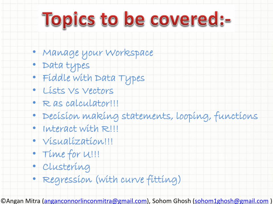
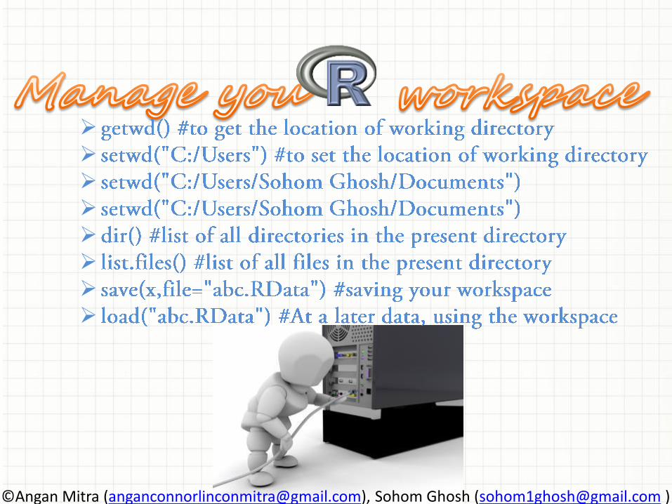
• Manage your Workspace • Data types • Fiddle with Data Types • Lists Vs Vectors • R as calculator!!! • Decision making statements, looping, functions • Interact with R!!! • Visualization!!! • Time for U!!! • Clustering • Regression (with curve fitting)
©Angan Mitra ([email protected]), Sohom Ghosh ([email protected] )

©Angan Mitra ([email protected]), Sohom Ghosh ([email protected] )
©Angan Mitra ([email protected]), Sohom Ghosh ([email protected] )
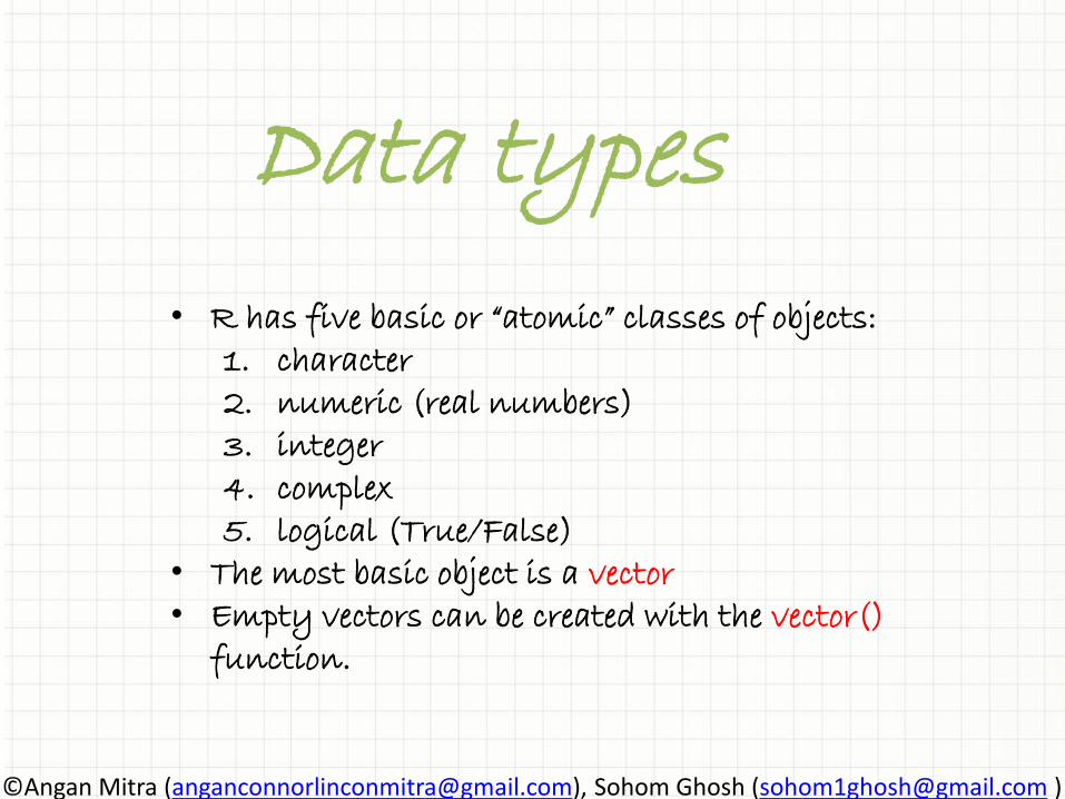
Data types
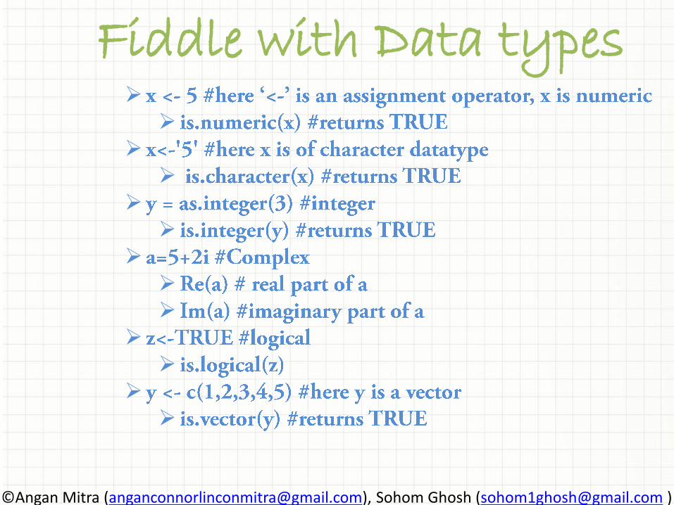
• R has five basic or “atomic” classes of objects: 1. character 2. numeric (real numbers) 3. integer 4. complex 5. logical (True/False)
• The most basic object is a vector • Empty vectors can be created with the vector()
function.
©Angan Mitra ([email protected]), Sohom Ghosh ([email protected] )
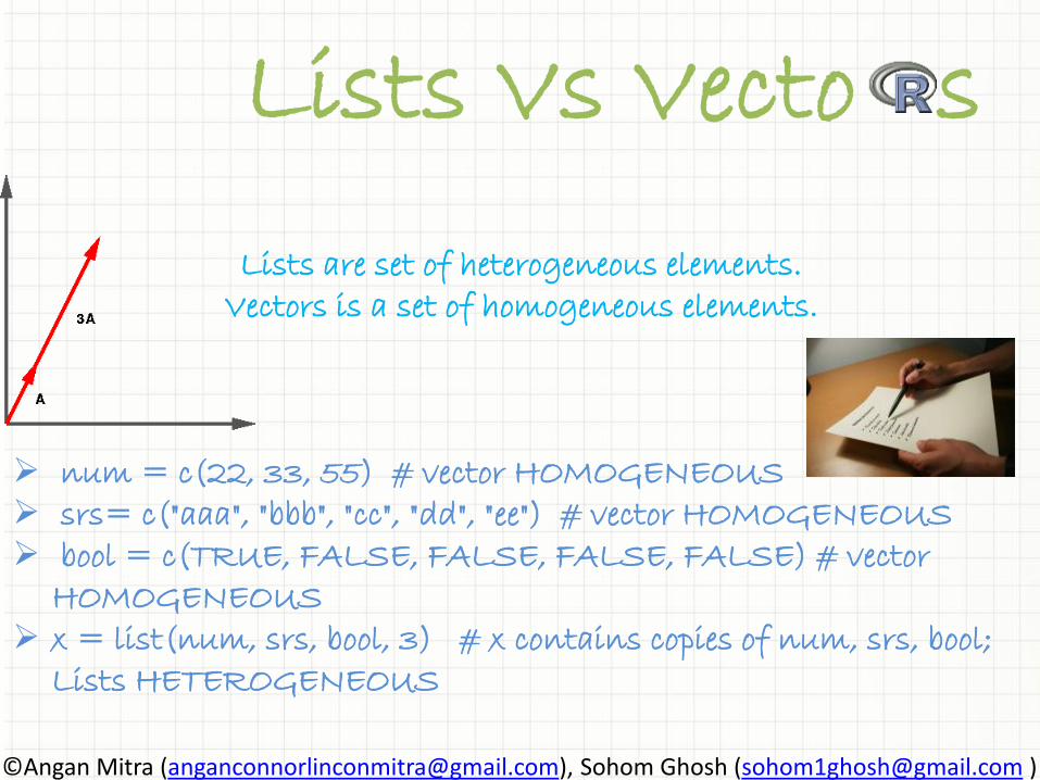
Lists Vs Vecto s
Lists are set of heterogeneous elements. Vectors is a set of homogeneous elements.
num = c(22, 33, 55) # vector HOMOGENEOUS srs= c("aaa", "bbb", "cc", "dd", "ee") # vector HOMOGENEOUS bool = c(TRUE, FALSE, FALSE, FALSE, FALSE) # vector
HOMOGENEOUS x = list(num, srs, bool, 3) # x contains copies of num, srs, bool;
Lists HETEROGENEOUS
©Angan Mitra ([email protected]), Sohom Ghosh ([email protected] )
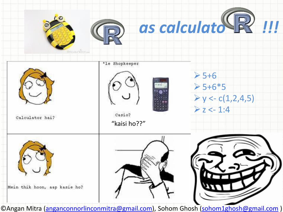
as calculato !!!
5+6 5+6*5 y <- c(1,2,4,5) z <- 1:4
“kaisi ho??”
©Angan Mitra ([email protected]), Sohom Ghosh ([email protected] )
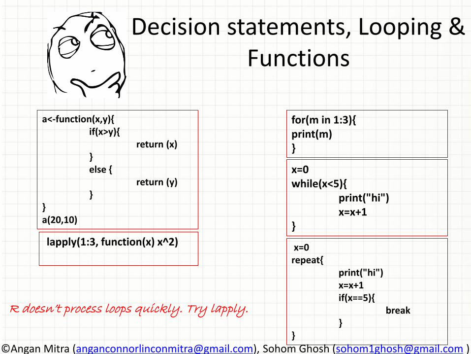
Decision statements, Looping & Functions
a<-function(x,y){ if(x>y){ return (x) } else { return (y) } } a(20,10)
for(m in 1:3){ print(m) }
x=0 while(x<5){ print("hi") x=x+1 }
lapply(1:3, function(x) x^2)
x=0 repeat{ print("hi") x=x+1 if(x==5){ break } }
R doesn’t process loops quickly. Try lapply.
©Angan Mitra ([email protected]), Sohom Ghosh ([email protected] )
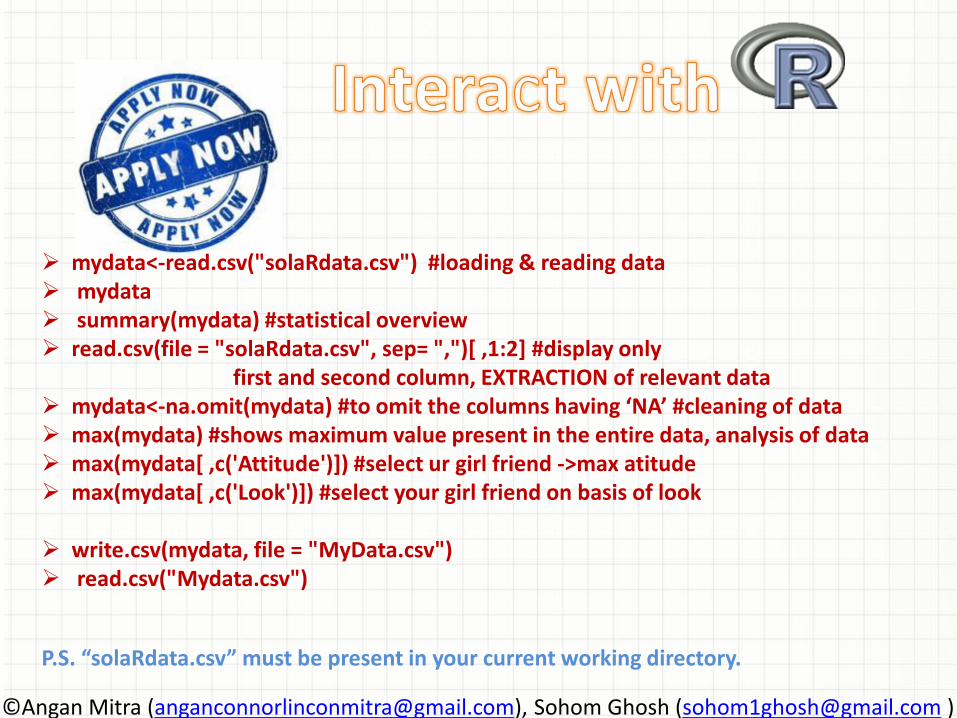
mydata<-read.csv("solaRdata.csv") #loading & reading data mydata summary(mydata) #statistical overview read.csv(file = "solaRdata.csv", sep= ",")[ ,1:2] #display only first and second column, EXTRACTION of relevant data mydata<-na.omit(mydata) #to omit the columns having ‘NA’ #cleaning of data max(mydata) #shows maximum value present in the entire data, analysis of data max(mydata[ ,c('Attitude')]) #select ur girl friend ->max atitude max(mydata[ ,c('Look')]) #select your girl friend on basis of look
write.csv(mydata, file = "MyData.csv") read.csv("Mydata.csv")
P.S. “solaRdata.csv” must be present in your current working directory.
©Angan Mitra ([email protected]), Sohom Ghosh ([email protected] )
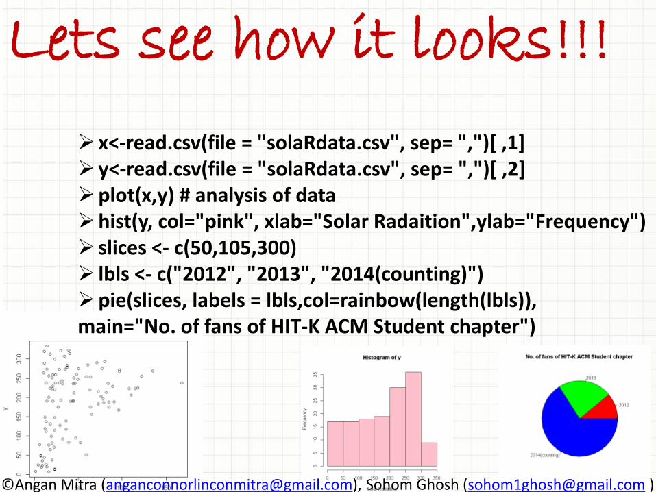
Lets see how it looks!!!
x<-read.csv(file = "solaRdata.csv", sep= ",")[ ,1] y<-read.csv(file = "solaRdata.csv", sep= ",")[ ,2] plot(x,y) # analysis of data hist(y, col="pink", xlab="Solar Radaition",ylab="Frequency") slices <- c(50,105,300) lbls <- c("2012", "2013", "2014(counting)") pie(slices, labels = lbls,col=rainbow(length(lbls)), main="No. of fans of HIT-K ACM Student chapter")
©Angan Mitra ([email protected]), Sohom Ghosh ([email protected] )

Its time fo U!!!!
1. Display first and second rows of solaRdata.csv
2. Display the minimum value present in the entire dataset
3. Find maximum element in First row
©Angan Mitra ([email protected]), Sohom Ghosh ([email protected] )
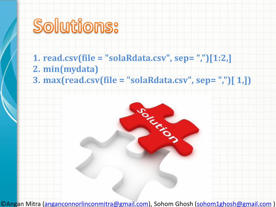
1. read.csv(file = "solaRdata.csv", sep= ",")[1:2,] 2. min(mydata) 3. max(read.csv(file = "solaRdata.csv", sep= ",")[ 1,])
©Angan Mitra ([email protected]), Sohom Ghosh ([email protected] )
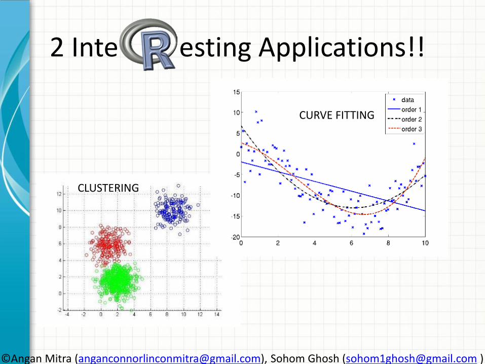
2 Inte esting Applications!!
CLUSTERING
CURVE FITTING
©Angan Mitra ([email protected]), Sohom Ghosh ([email protected] )
Curve Fitting
• Curve fitting is the process of constructing a curve, or mathematical function, that has the best fit to a series of data points, possibly subject to constraints.
If you just had a feel its like the ones you learn in your degree courses…….here is some you can try hands on..
©Angan Mitra ([email protected]), Sohom Ghosh ([email protected] )
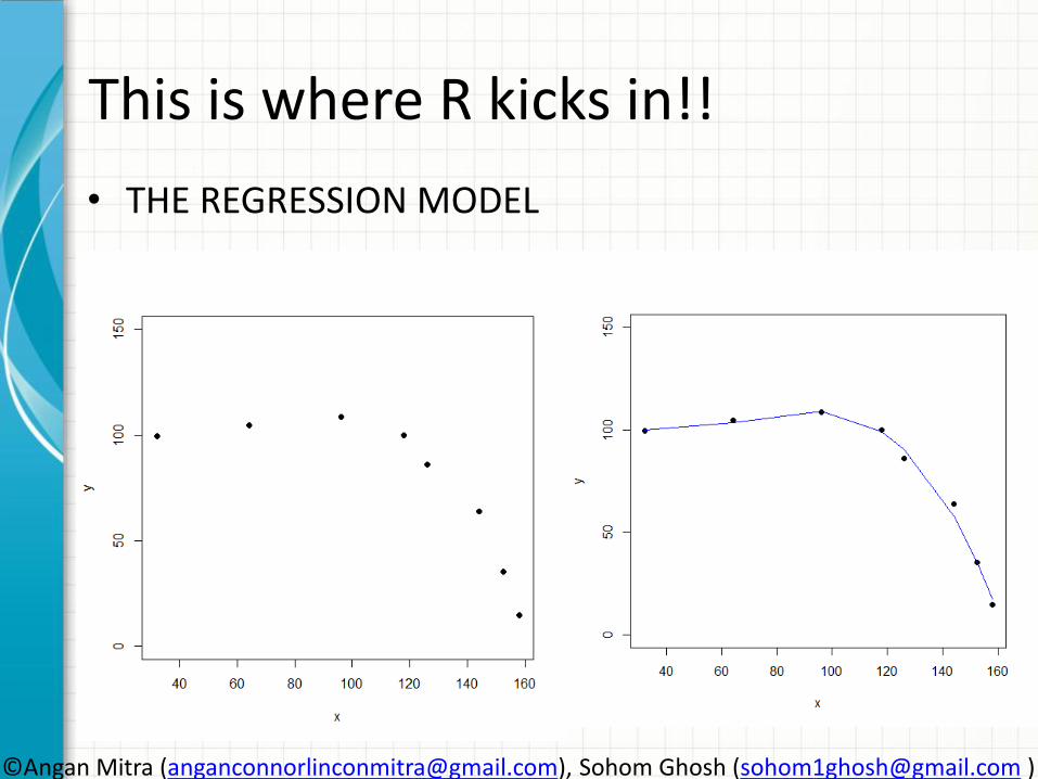
This is where R kicks in!!
• THE REGRESSION MODEL
©Angan Mitra ([email protected]), Sohom Ghosh ([email protected] )
©Angan Mitra ([email protected]), Sohom Ghosh ([email protected] )
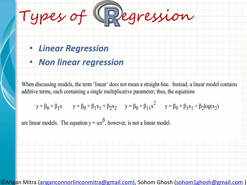
Types of egression
• Linear Regression
• Non linear regression
©Angan Mitra ([email protected]), Sohom Ghosh ([email protected] )
THE DATA: mydata<-read.csv(“Rdata.csv”) newdata <- mydata[,1:2] print(newdata) y<-newdata[,2] x<-newdata[,1] plot(x,y)
©Angan Mitra ([email protected]), Sohom Ghosh ([email protected] )
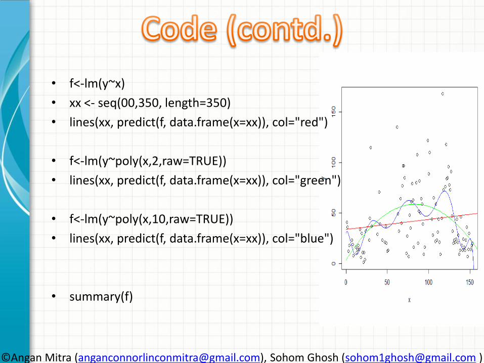
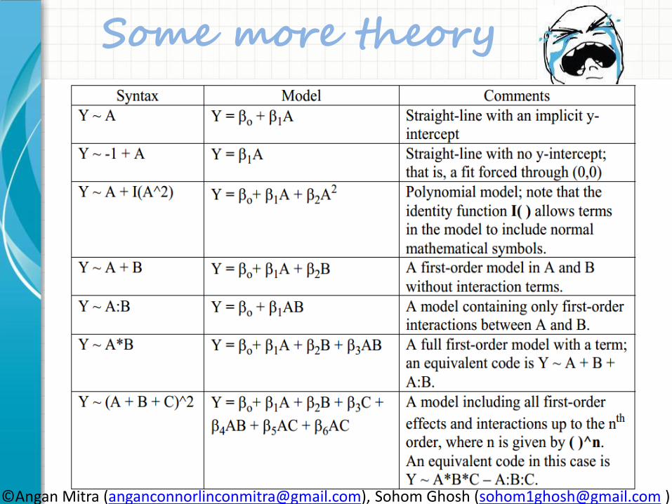
• f<-lm(y~x)
• xx <- seq(00,350, length=350)
• lines(xx, predict(f, data.frame(x=xx)), col="red")
• f<-lm(y~poly(x,2,raw=TRUE))
• lines(xx, predict(f, data.frame(x=xx)), col="green")
• f<-lm(y~poly(x,10,raw=TRUE))
• lines(xx, predict(f, data.frame(x=xx)), col="blue")
• summary(f)
©Angan Mitra ([email protected]), Sohom Ghosh ([email protected] )

luste
Many to pick from!!
–Connectivity based clustering
–Centroid based clustering
–Distribution based clustering
–Density based clustering
–A Lot more…
©Angan Mitra ([email protected]), Sohom Ghosh ([email protected] )
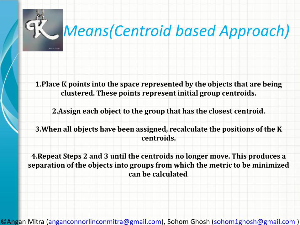
Means(Centroid based Approach)
1.Place K points into the space represented by the objects that are being clustered. These points represent initial group centroids.
2.Assign each object to the group that has the closest centroid.
3.When all objects have been assigned, recalculate the positions of the K
centroids.
4.Repeat Steps 2 and 3 until the centroids no longer move. This produces a separation of the objects into groups from which the metric to be minimized
can be calculated.
©Angan Mitra ([email protected]), Sohom Ghosh ([email protected] )
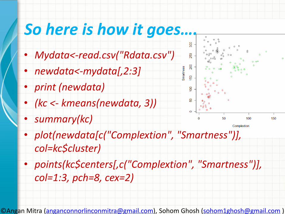
So here is how it goes….
• Mydata<-read.csv("Rdata.csv")
• newdata<-mydata[,2:3]
• print (newdata)
• (kc <- kmeans(newdata, 3))
• summary(kc)
• plot(newdata[c("Complextion", "Smartness")], col=kc$cluster)
• points(kc$centers[,c("Complextion", "Smartness")], col=1:3, pch=8, cex=2)
©Angan Mitra ([email protected]), Sohom Ghosh ([email protected] )

Bibliography
• http://www.slidesshare.net
• http://images.google.com/
• http://en.wikipedia.org
• http://cran.r-project.org/
• http://www.statmethods.net/
©Angan Mitra ([email protected]), Sohom Ghosh ([email protected] )
©Angan Mitra ([email protected]), Sohom Ghosh ([email protected] )