R package bsts - Prof. Hedibert Freitas Lopes, PhD |...

R package bstsBayesian structural time series

Uses Markov Chain Monte Carlo to sample from the posteriordistribution of a Bayesian structural time series model.

Author: Steven L. Scott - [email protected]

References:

Harvey (1990) Forecasting, structural time series, and the Kalman filter

Durbin and Koopman (2001) Time series analysis by state space methods

Scott and Varian (2013) Predicting the Present with Bayesian Structural Time Serieshttp://people.ischool.berkeley.edu/~hal/Papers/2013/pred-present-with-bsts.pdf

1 / 12

http://people.ischool.berkeley.edu/~hal/Papers/2013/pred-present-with-bsts.pdf

Usage

bsts(formula,

state.specification,

family = c("gaussian", "logit", "poisson", "student"),

save.state.contributions = TRUE,

save.prediction.errors = TRUE,

data,

bma.method = c("SSVS", "ODA"),

prior,

oda.options = list(

fallback.probability = 0.0,

eigenvalue.fudge.factor = 0.01),

contrasts = NULL,

na.action = na.pass,

niter,

ping = niter / 10,

timeout.seconds = Inf,

seed = NULL,

...)

2 / 12

add.local.linear.trend

Add a local linear trend model to a state specification:

µt = µt−1 + δt−1 + ω1t ω1t ∼ N(0, σ2level)

δt = δt−1 + ω2t ω2t ∼ N(0, σ2slope)

The prior distribution is on σlevel and σslope.

AddLocalLinearTrend(

state.specification = NULL,

y,

level.sigma.prior = NULL,

slope.sigma.prior = NULL,

initial.level.prior = NULL,

initial.slope.prior = NULL,

sdy,

initial.y)

3 / 12

add.seasonalAdd a seasonal model to a state specification.The seasonal model can be thought of as a regression onnseasons dummy variables with coefficients constrained to sum to1 (in expectation). If there are S seasons then the state vectorgamma is of dimension S − 1:

γ1t = −S−1∑s=1

γs,t−1 + ω3t ω3t ∼ N(0, σ2seas)

γst = γs−1,t−1 s = 2, . . . , S − 1.

AddSeasonal(

state.specification,

y,

nseasons,

season.duration = 1,

sigma.prior,

initial.state.prior,

sdy)

4 / 12

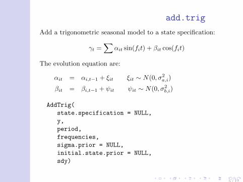
add.trig

Add a trigonometric seasonal model to a state specification:

γt =∑

αit sin(fit) + βit cos(fit)

The evolution equation are:

αit = αi,t−1 + ξit ξit ∼ N(0, σ2a,i)

βit = βi,t−1 + ψit ψit ∼ N(0, σ2b,i)

AddTrig(

state.specification = NULL,

y,

period,

frequencies,

sigma.prior = NULL,

initial.state.prior = NULL,

sdy)

5 / 12

Airline data

Time

y

1950 1952 1954 1956 1958 1960

5.0

5.5

6.0

6.5

yt = µt + γ1t + vt vt ∼ N(0, σ2obs)

µt = µt−1 + δt−1 + ω1t ω1t ∼ N(0, σ2level)

δt = δt−1 + ω2t ω2t ∼ N(0, σ2slope)

γ1t = −S−1∑s=1

γs,t−1 + ω3t ω3t ∼ N(0, σ2seas)

γst = γs−1,t−1 s = 2, . . . , S − 1.

6 / 12

install.packages("bsts")

library(bsts)

data(AirPassengers)

y = log(AirPassengers)

ss = AddLocalLinearTrend(list(), y)

ss = AddSeasonal(ss, y, nseasons = 12)

model = bsts(y, state.specification = ss, niter = 10000)

=-=-=-=-= Iteration 0 Sat May 7 14:45:34 2016 =-=-=-=-=




names(model)

[1] "sigma.obs" "sigma.trend.level"

[3] "sigma.trend.slope" "sigma.seasonal.12"

[5] "final.state" "state.contributions"

[7] "one.step.prediction.errors" "log.likelihood"

[9] "has.regression" "state.specification"

[11] "family" "niter"

[13] "original.series"

dim(model$state.contributions)

[1] 10000 2 144

7 / 12

Posterior of(σobs, σlevel, σslope, σseas)

sigmas = cbind(model$sigma.obs,

model$sigma.trend.level,

model$sigma.trend.slope,

model$sigma.seasonal.12)

round(cbind(apply(sigmas[5001:10000,],2,mean),

apply(sigmas[5001:10000,],2,median),

apply(sigmas[5001:10000,],2,quantile,0.025),

apply(sigmas[5001:10000,],2,quantile,0.975)),4)

[,1] [,2] [,3] [,4]

[1,] 0.0269 0.0267 0.0201 0.0346

[2,] 0.0061 0.0054 0.0031 0.0139

[3,] 0.0045 0.0044 0.0033 0.0061

[4,] 0.0107 0.0107 0.0030 0.0176

pdf(file="bsts-graph1.pdf",width=10,height=7)

par(mfrow=c(3,4))

for (i in 1:4)

ts.plot(sigmas[,i],ylab="")

for (i in 1:4)

acf(sigmas[5001:10000,i],main="")

for (i in 1:4)

hist(sigmas[5001:10000,i],xlab="",main="",prob=TRUE)

dev.off()

8 / 12

(σobs, σlevel, σslope, σseas)

Time

0 2000 6000 10000

0.02

0.06

0.10

Time

0 2000 6000 10000

0.00

50.

015

Time

0 2000 6000 10000

0.00

30.

006

0.00

9

Time

0 2000 6000 10000

0.00

50.

015

0 5 10 15 20 25 30 35

0.0

0.4

0.8

Lag

AC

F

0 5 10 15 20 25 30 35

0.0

0.4

0.8

Lag

AC

F

0 5 10 15 20 25 30 35

0.0

0.4

0.8

Lag

AC

F

0 5 10 15 20 25 30 35

0.0

0.4

0.8

Lag

AC

F

Den

sity

0.015 0.025 0.035 0.045

020

6010

0

Den

sity

0.005 0.015

050

100

200

Den

sity

0.003 0.005 0.007

020

040

0

Den

sity

0.005 0.010 0.015 0.020

040

8012

0

9 / 12

Posterior of σs

components = cbind.data.frame(

colMeans(model$state.contributions[-(1:5000),"trend",]),

colMeans(model$state.contributions[-(1:5000),"seasonal.12.1",]),

as.Date(time(y)))

names(components) = c("Trend", "Seasonality", "Date")

components = melt(components, id="Date")

names(components) = c("Date", "Component", "Value")

pdf(file="bsts-graph2.pdf",width=10,height=7)

ggplot(data=components, aes(x=Date, y=Value)) + geom_line() +

theme_bw() + theme(legend.title = element_blank()) + ylab("") + xlab("") +

facet_grid(Component ~ ., scales="free") + guides(colour=FALSE) +

theme(axis.text.x=element_text(angle = -90, hjust = 0))

dev.off()

10 / 12

Free-form seasonality

4.8

5.2

5.6

6.0

−0.2

−0.1

0.0

0.1

0.2

TrendS

easonality

1950

1952

1954

1956

1958

1960

11 / 12

Trigonometric seasonality

5.0

5.5

6.0

−0.3

−0.2

−0.1

0.0

0.1

0.2

0.3

TrendS

easonality

1950

1952

1954

1956

1958

1960

12 / 12

R package bsts - Prof. Hedibert Freitas Lopes, PhD |...

Documents

Transcript of R package bsts - Prof. Hedibert Freitas Lopes, PhD |...