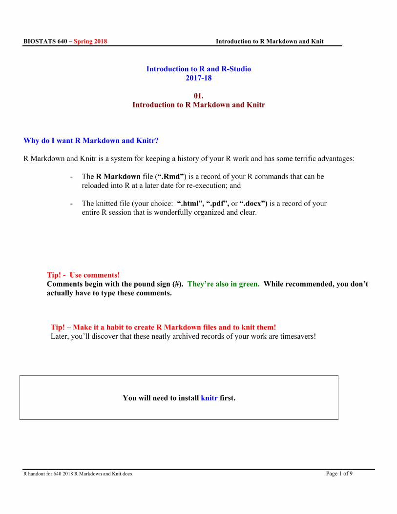
BIOSTATS 640 – Spring 2018 Introduction to R Markdown and Knit

R handout for 640 2018 R Markdown and Knit.docx Page 1 of 9

Introduction to R and R-Studio 2017-18

01.

Introduction to R Markdown and Knitr

Why do I want R Markdown and Knitr? R Markdown and Knitr is a system for keeping a history of your R work and has some terrific advantages:

- The R Markdown file (“.Rmd”) is a record of your R commands that can be reloaded into R at a later date for re-execution; and

- The knitted file (your choice: “.html”, “.pdf”, or “.docx”) is a record of your entire R session that is wonderfully organized and clear.

Tip! - Use comments! Comments begin with the pound sign (#). They’re also in green. While recommended, you don’t actually have to type these comments.

Tip! – Make it a habit to create R Markdown files and to knit them! Later, you’ll discover that these neatly archived records of your work are timesavers!

You will need to install knitr first.

BIOSTATS 640 – Spring 2018 Introduction to R Markdown and Knit

R handout for 640 2018 R Markdown and Knit.docx Page 2 of 9

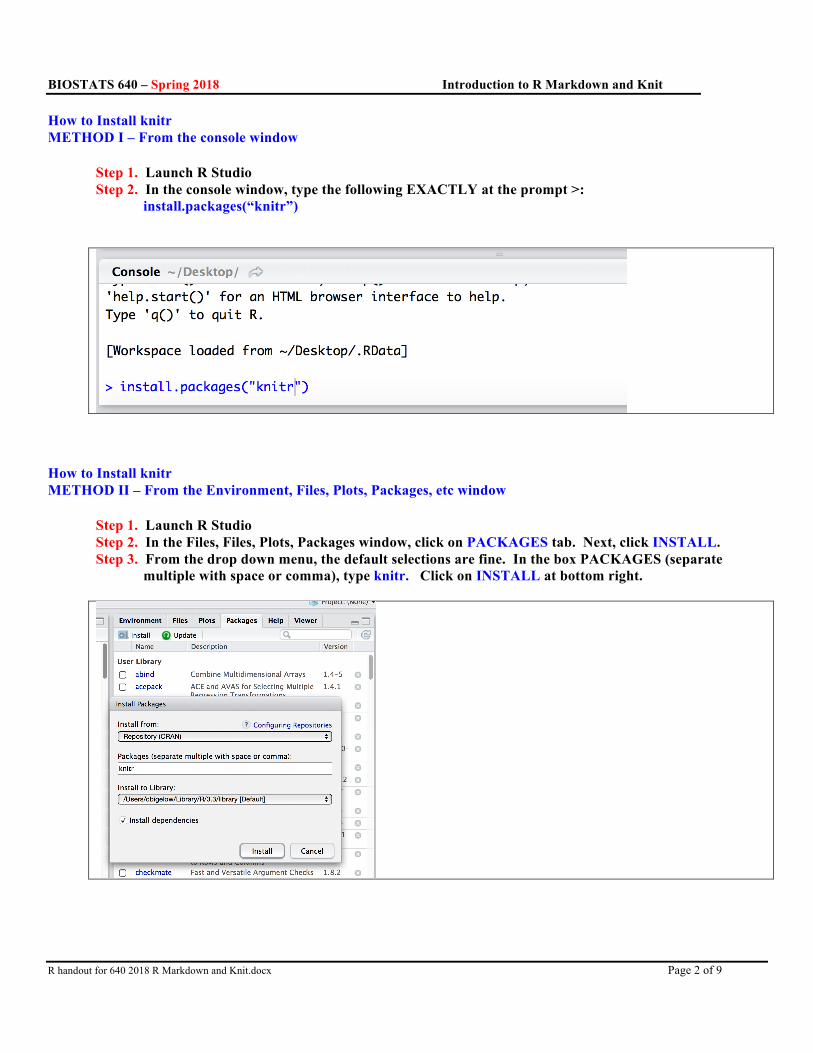
How to Install knitr METHOD I – From the console window

Step 1. Launch R Studio Step 2. In the console window, type the following EXACTLY at the prompt >: install.packages(“knitr”)

How to Install knitr METHOD II – From the Environment, Files, Plots, Packages, etc window

Step 1. Launch R Studio Step 2. In the Files, Files, Plots, Packages window, click on PACKAGES tab. Next, click INSTALL. Step 3. From the drop down menu, the default selections are fine. In the box PACKAGES (separate multiple with space or comma), type knitr. Click on INSTALL at bottom right.

BIOSTATS 640 – Spring 2018 Introduction to R Markdown and Knit

R handout for 640 2018 R Markdown and Knit.docx Page 3 of 9

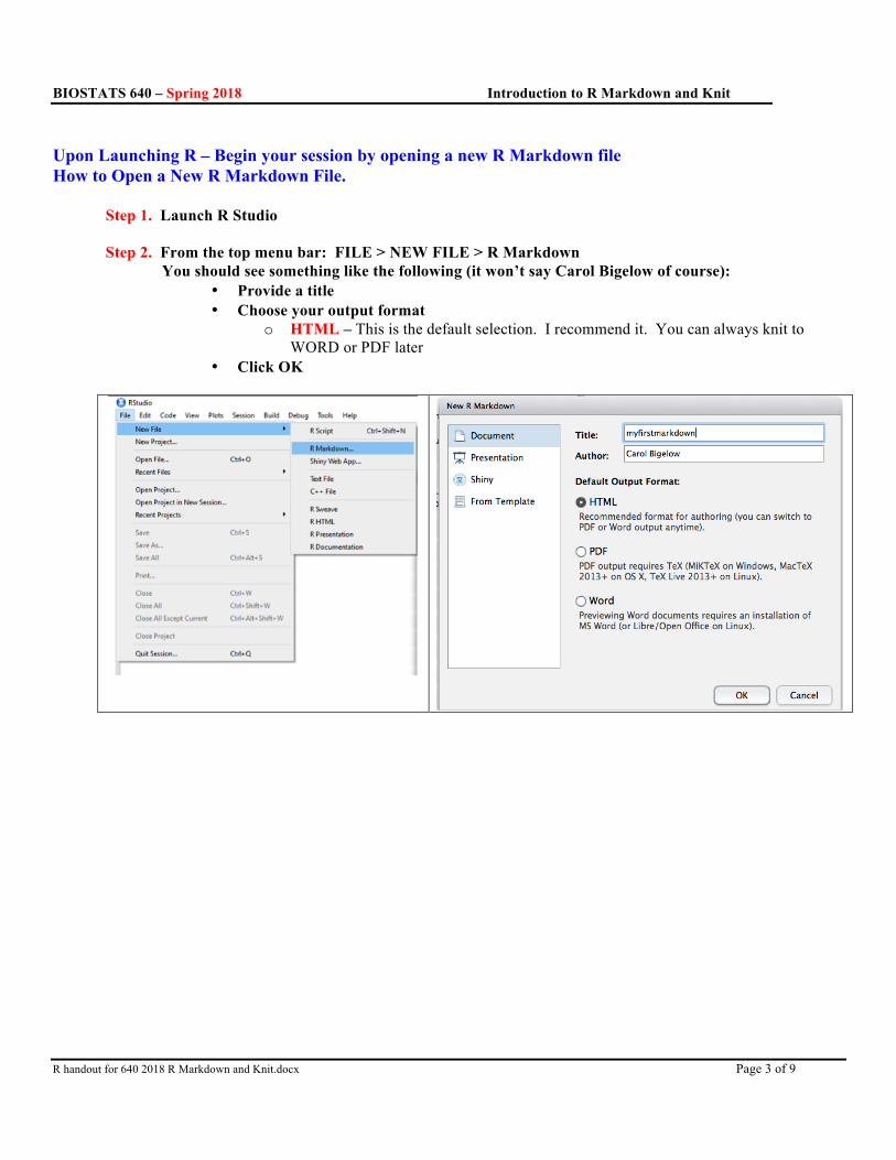
Upon Launching R – Begin your session by opening a new R Markdown file How to Open a New R Markdown File.

Step 1. Launch R Studio Step 2. From the top menu bar: FILE > NEW FILE > R Markdown You should see something like the following (it won’t say Carol Bigelow of course):

• Provide a title • Choose your output format

o HTML – This is the default selection. I recommend it. You can always knit to WORD or PDF later

• Click OK

BIOSTATS 640 – Spring 2018 Introduction to R Markdown and Knit

R handout for 640 2018 R Markdown and Knit.docx Page 4 of 9

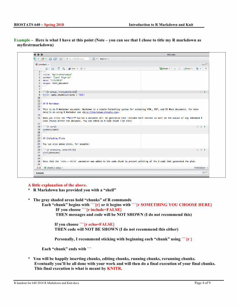
Example – Here is what I have at this point (Note – you can see that I chose to title my R markdown as myfirstrmarkdown)

A little explanation of the above. * R Markdown has provided you with a “shell” * The gray shaded areas hold “chunks” of R commands Each “chunk” begins with ```{r} or it begins with ```{r SOMETHING YOU CHOOSE HERE} IF you choose ```{r include=FALSE} THEN messages and code will be NOT SHOWN (I do not recommend this) If you choose ```{r echo=FALSE} THEN code will NOT BE SHOWN (I do not recommend this either) Personally, I recommend sticking with beginning each “chunk” using ```{r } Each “chunk” ends with ``` * You will be happily inserting chunks, editing chunks, running chunks, rerunning chunks. Eventually you’ll be all done with your work and will then do a final execution of your final chunks. This final execution is what is meant by KNITR.

BIOSTATS 640 – Spring 2018 Introduction to R Markdown and Knit

R handout for 640 2018 R Markdown and Knit.docx Page 5 of 9

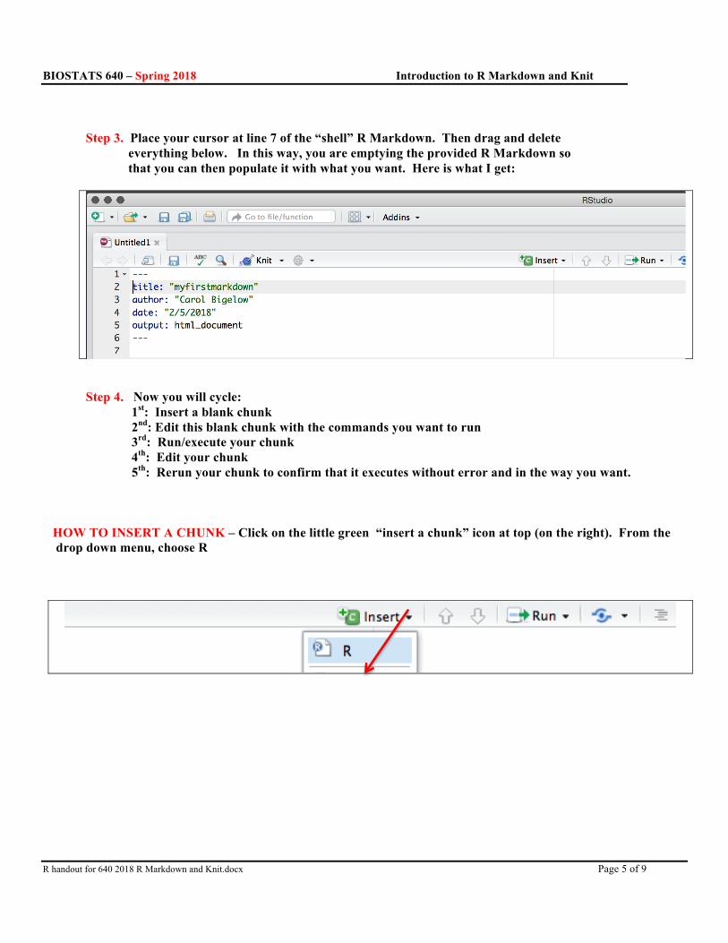
Step 3. Place your cursor at line 7 of the “shell” R Markdown. Then drag and delete everything below. In this way, you are emptying the provided R Markdown so that you can then populate it with what you want. Here is what I get:

Step 4. Now you will cycle: 1st: Insert a blank chunk 2nd: Edit this blank chunk with the commands you want to run 3rd: Run/execute your chunk 4th: Edit your chunk 5th: Rerun your chunk to confirm that it executes without error and in the way you want.

HOW TO INSERT A CHUNK – Click on the little green “insert a chunk” icon at top (on the right). From the drop down menu, choose R

BIOSTATS 640 – Spring 2018 Introduction to R Markdown and Knit

R handout for 640 2018 R Markdown and Knit.docx Page 6 of 9

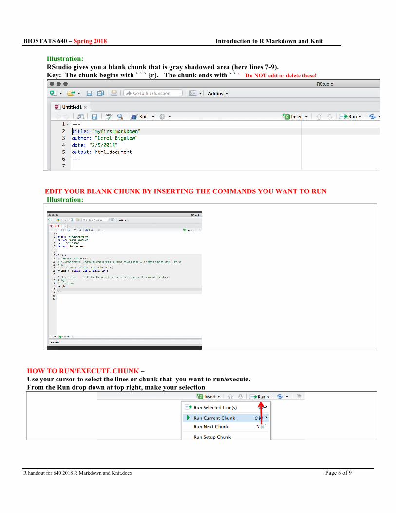
Illustration: RStudio gives you a blank chunk that is gray shadowed area (here lines 7-9). Key: The chunk begins with ` ` ` {r}. The chunk ends with ` ` ` Do NOT edit or delete these!

EDIT YOUR BLANK CHUNK BY INSERTING THE COMMANDS YOU WANT TO RUN

Illustration:

HOW TO RUN/EXECUTE CHUNK – Use your cursor to select the lines or chunk that you want to run/execute. From the Run drop down at top right, make your selection

BIOSTATS 640 – Spring 2018 Introduction to R Markdown and Knit

R handout for 640 2018 R Markdown and Knit.docx Page 7 of 9

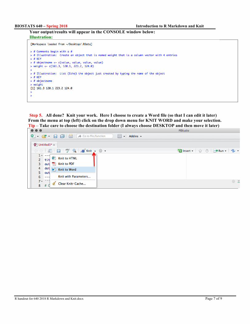
Your output/results will appear in the CONSOLE window below: Illustration:

Step 5. All done? Knit your work. Here I choose to create a Word file (so that I can edit it later)

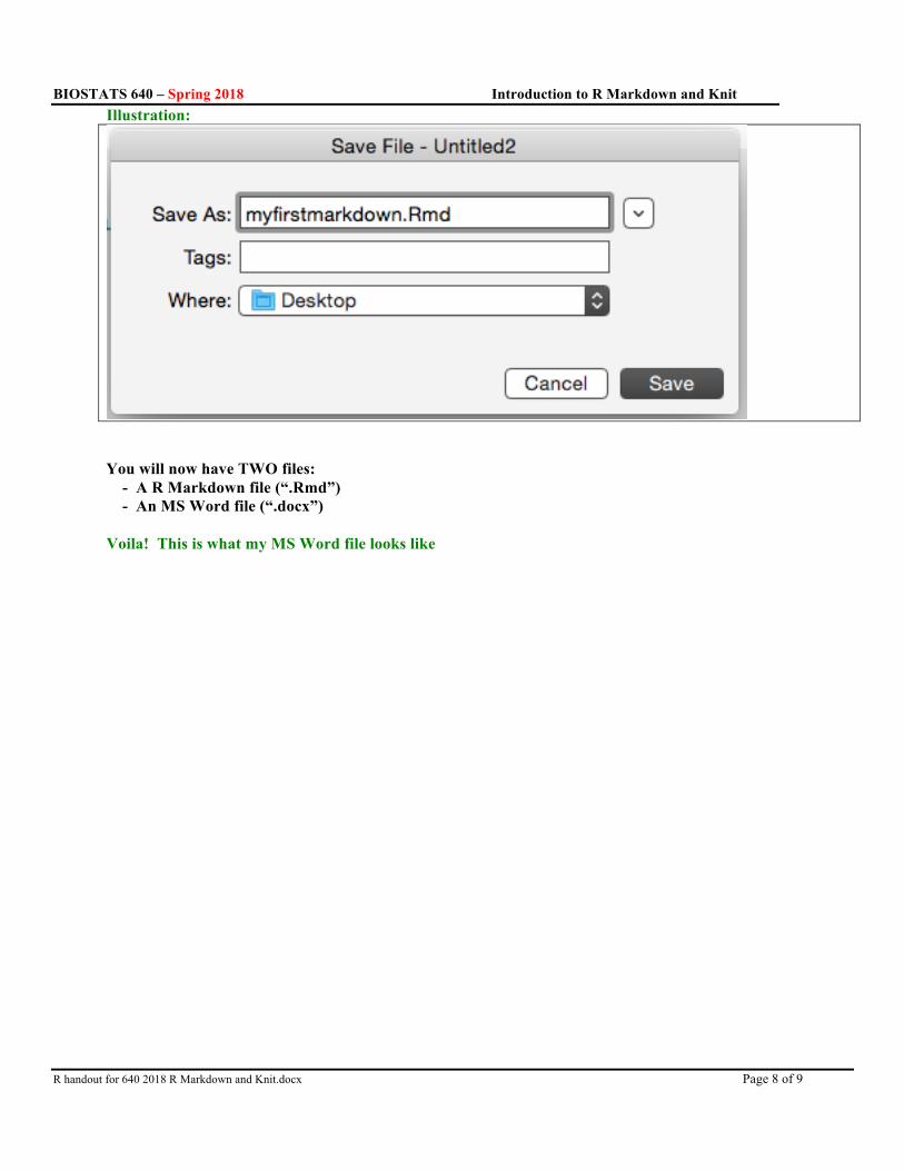
From the menu at top (left) click on the drop down menu for KNIT WORD and make your selection. Tip – Take care to choose the destination folder (I always choose DESKTOP and then move it later)

BIOSTATS 640 – Spring 2018 Introduction to R Markdown and Knit

R handout for 640 2018 R Markdown and Knit.docx Page 8 of 9

Illustration:

You will now have TWO files: - A R Markdown file (“.Rmd”) - An MS Word file (“.docx”)

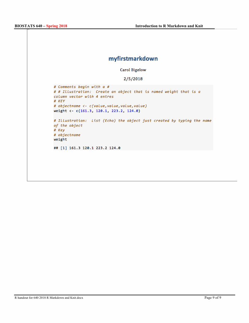
Voila! This is what my MS Word file looks like

BIOSTATS 640 – Spring 2018 Introduction to R Markdown and Knit

R handout for 640 2018 R Markdown and Knit.docx Page 9 of 9