R. H. Gooding November 1970 - dtic.mil · ROYAL AIRCRAFT ESTABLISHMENT Technical Memorandum Space...

>

BR22997 TECH. MEMO SPACE 157

TECH. MEMO SPACE 157

(M 1> (M 00 ROYAL AI R C R A F T ESTABLISHMENT

CQ r- IS

APPLICATIONS AND RESULTS OF ORBIT DETERMINATION

by

R. H. Gooding

November 1970

* * r<-

üj -- f.,..

Roproducod by

NATIONAL TECHNICAL INFORMATION SERVICE

Sprinslield, Vl illSI

Crown Copyright 1970

i » f

■

v] tt

'

ROYAL AIRCRAFT ESTABLISHMENT

Technical Memorandum Space 157

November 1970

APPLICATIONS AND RESULTS OF ORBIT DETERMINATION

by

R. H. Gooding

SUMMARY

This paper summarizes the reasons for determining the orbits of earth

satellites, and describes how knowledge of the earth's gravitational

potential and its atmosphere has improved as a result of orbit determination.

The paper is based on the second of two lectures given at the ESRO summer

school on Spacecraft Operations, held at Gravenbruch, near Frankfurt,

West Germany, in August 1970. The first lecture is available as

Technical Memorandum Space 156.

SP 157

1 INTRODUCTION

In the first of my two lectures I gave some technical details of orbit

determination by the method of differential correction, with special

reference to the computer programs that have been developed at the

Royal Aircraft Establishment. In this remaining lecture I propose to list

and discuss briefly the main reasons why orbit determination is necessary at

all, and then to elaborate on the last two topics in the list.

2 OBJECTIVES OF ORBIT DETERMINATION

Fig.l is based on Merson's classification of the objectives of orbit

determination as operational and non-operational. The distinction between

the two classes is that the former are essential to the particular

satellite, whereas the latter are not, but this distinction is not always

clear-cut.

Orbit achievement may seem too obvious an objective to include in the

list. It is too important to omit, however; until a satellite has been

tracked, there is no certainty that it is in orbit, and until a rough orbit

has been computed from tracking data, there is no certainty that the orbit

is satisfactory. Again, the performance of the launching vehicle can only

be properly evaluated when the resulting orbit is known.

Guidance and control will be required, in particular, for communica-

tion satellites and space probes. The correct commands to change an orbit

cannot be made until the current orbit is known.

On-board instrumentation plays a vital role for scientific satellites

such as the Ariels. The telemetered data from such instrumentation must

usually be correlated with satellite position (for example to plot electron

density against height and latitude), and continuous knowledge of satellite

position can only come from orbit determination.

Tracking and telemetry scheduling, for the various stations in a

network, require knowledge of the orbit, and the stations will need

predicted look angles for the scheduled passes. The accuracy desired for

this objective is usually much less than for the previous one, but the

urgency is of course much greater.

General surveillance, the first non-operational objective listed, is

required in both a military and a technical context. The military require-

ment is to monitor all spacecraft and to detect, as rapidly as possible,

SP 157

any object newly launched into orbit. The technical requirement is to dis-

tinguish one satellite from another, in particular to avoid interference

when communicating with a given satellite.

Sensor accuracy, i.e. the accuracy of the instrumentation at a given

satellite observing station, can be estimated by consideration of the

equipment itself, but auch estimation can only be validated by studying

residuals of actual satellite observations relative to computed orbits.

Navigation and geodesy could as well appear under 'operational

objectives', since a number of satellites have been launched with these

objectives specifically in mind. The US Navy has refined a navigation

system based on Doppler measurement of range rate, in which the orbit of a

satellite is determined from Doppler observations from a standard network

of ground stations. The resulting orbital parameters are fed into the

satellite itself, which transmits them continuously (until a further set

is fed in). Then a ship, using relatively simple equipment, can track the

satellite and, from the observed Doppler shift and the orbital parameters,

can locate its own position. Geodesy, however, has certainly been mainly

associated with non-operational objectives. Here I am not thinking of the

'direct' or 'geometrical' method of approach, which is based on the

simultaneous observation of a satellite from two or more stations which

have been accurately surveyed relative to the same datum and from a station

which it is required to survey to this datum, since this method does not

require an orbit to be determined. I am thinking rather of the 'indirect'

or 'orbital' method in which one has available a vast number of accurate

observations of several satellites, and can therefore carry out a simul-

taneous differential correction, not merely of the parameters of all the

satellites, but also of the sets of station coordinates. The best known

contributions to satellite geodesy to date have probably been the 1966 2 9

and 1969 Smithsonian Standard Earths ' , for which the observational data

♦.are obtained mainly from Baker-Nunn cameras.

The last two non-operational objectives, concerned with improved

knowledge of the earth's gravitational field and of atmospheric density

and rotation, are my two main topics, to be covered in some detail in the

following sections. The first of these objectives is related to the

geodesy objective, the difference being that an even broader view is taken -

we are concerned with the gravitational constants of the solid earth and not

merely with the surveying of its surface. Only an 'indirect method' is

possible.

SP 157

The same principle is involved in the orbit-based study of both the

earth's gravitational field and its atmosphere, namely that orbits suffer

'perturbations' as I indicated in my first lecture. Such perturbations

may be represented by a mathematical theory - the 'orbital model' or

'orbit generator' - and the numerical parameters of this theory may be

inferred from observation of the perturbations.

It is important to realise that the method depends not only on the

study of the orbits of a number of satellites but also, usually, on a

large number of orbit determinations, over a long period, for each satellite.

The principle is illustrated in Fig.2. Here an existing orbital model is

assumed to be good enough to describe the motion of a satellite during a

short period, i.e. good enough for orbit determination over such a period to

yield pmall final residuals. After many orbit determinations for the same

satellite, over a long period, the graph of one of the orbital parameters is

plotted, its variation being due to perturbations. The existing orbital

model gives a poor fit to this long-term variation of the orbital parameter,

but the fit may be dramatically improved by use of revised earth constants in

the model. Alternatively, it may be that an improved model, incorporating

previously neglected perturbations, is required before an adequate fit can be

obtained.

It is fortunate that gravity-induced perturbations have a very different

character from atmosphere-induced perturbations. This means that the two

subjects can essentially be considered independently, as I now proceed to do.

3 GRAVITATIONAL FIELD OF THE EARTH

If the earth were spherically symmetrical its field would be the same

as that of a point mass as its centre; i.e. satellite motion would be

unperturbed. Thus gravity-induced perturbations yield information about

asphericity.

The simplest improvement upon an assumption of sphericity is to take

the earth as an oblate spheroid. This is illustrated in Fig.3. The

'flattening* of such a spheroid is defined, in terms of the polar and

equatorial diameters, by the relation

SP 157

here flattening must not be confused with eccentricity, a term not usually

used in this context but which would be defined by

2 2 2 DE-DP e

"l The first estimate of f was by Newton who, by theoretical argument,

obtained the value 1/230. After the development of refined geodetic methods,

Hayford gave the value 1/297.0 in 1909, and this was adopted as an

international standard in 192A. The current best value, based on orbit

determination, is 1/298.25, so that Hayford overestimated the difference

between D and D , which is about A3 km, by some 180 metres.

The next improvement in the assumption about the earth's shape, made

worthwhile by the advent of satellites, is to take it as axisymmetric, so

that the gravitational potential is latitude-dependent but longitude-

independent. From the fact that the potential must satisfy Laplace's

equation it follows that the most general form, subject to axial symmetry,

is given by the Legcndre expansion

r ^\(sin3)J . 1 - Z V5I P« Csia 3)^ , (2)

where u is the product GM of the gravitational constant and the mass of

the earth, R is the equatorial radius of the~*arth, r is distance from

the earth's centre, 3 is geocentric latitude, P is the Legendre

polynomial of degree 2., and the 'zonal harmonic' coefficients J are

dimensionless constants which represent the shape of the earth. The first

coefficient in the series, J-, is directly related to the flattening, f,

but the relation is not as simple as might be expected, because JL is

associated with the gravitational field, whereas f is associated with the

gravity field (i.e. the gravitational field plus the centrifugal field on

the surface of the earth due to its rotation).

Fig.4 interprets the first four harmonics (J-, J-, J, and J.) as

distortions (from circularity) of a meridional cross-section of the earth.

The distortions are greatly exaggerated, and the shapes for J, and J. are

for positive values of these constants, whereas they are actually both negative.

Although all the zonal harmonics are axisymmetric, only the even harmonics -

SP 157

i.e. those for which i is even - are symmetric about the earth's equator.

Because the perturbations produced by the even harmonics are quite different

from those produced by the odd harmonics, it is usual to study them

separately.

Fig.5 gives values of the even harmonics, as determined by various 3 4 5

authors ' ' , and it is seen that there is good agreement as far as J,.

It is striking that, although J. is of order 10 , subsequent even —6

harmonics (and in fact all other harmonics) are of order 10 ; thus it is

not surprising that only J. could be estimated prior to the satellite 2

era. The fact that J (£. > 2) is of order J- is important in the

various theories of satellite perturbations in the earth's gravitational

field.

The main effects of the even zonal harmonics are on the orbital elements

n (right ascension of the node) and ui (argument of perigee). These have

secular perturbations, as I explained in my first lecture, and formulae for

their rates of change are

ft " " | J2 n (R/P)2 cos i + 0 (J4 etc.) (3)

and u> | J2 n (R/p)2 (4 - 5 sin2 i) + 0 (J4 etc.) , (4)

3 i 2 where n » (y/a ), i.e. n is the mean motion, p • a(l - e ), and the

remaining notation has already been given. Fig.6 illustrates ft as a

westward rotation of the orbital plane; this rotation vanishes only for

polar orbits. Similarly iL, interpreted as the rate of rotation of the

orbit within its plane, vanishes for inclinations such that sin i - +/0.8 .

These are the important 'critical inclinations', which are of both

theoretical and practical interest and which I referred to in my first

lecture. (Many Russian satellites have been launched with near-critical

inclination, so that perigee - or apogee for communication satellites -

might remain for long periods in the northern hemisphere.) It is from the

observed values of ft and u (or sometimes just from Q), averaged over

long periods for a number of satellites, that the even harmonic coefficients

are derived. Thus if the average value of ft observed for satellite A is

Ü., we have an equation of condition of the form

A2 J2 + A4 J4 + A6 J6 + •••• " "A '

SP 157

where A« = -1J n. (R/pA) cos i and fi. has been corrected by removal

of all the (small) effects of other sources of perturbations. Similar

equations of condition for satellites B, C etc. may be set up - it is

important that as wide a range of orbital inclinations as possible be

covered - and the whole set solved by the method of least squares. The 3

King-Hele/Cook solution was for four J coefficients, using seven

satellites.

Fig.7 gives values of the odd harmonics, one set determined by King-Hele,

Cook and Scott , and another set determined by Kozai . (Exactly zero-values

appear in the set of King-Hele et al., because in their first least-squares

solution they obtained such small values of these coefficients that they

dropped them altogether; having set nine odd J's to zero they determined

values of six others, using 22 satellites.) Agreement between the two sets

is good up to J7.

The odd harmonics do not lead to secular perturbations, so they are

determined from long-periodic perturbations, usually from the perturbations

in e (eccentricity). Fig.8, repeated from my first lecture, shows the

secular and long-periodic variation of e for the satellite Ariel 2. If

the secular variation is removed, the amplitude of the long-periodic

oscillation - of which the period is about 120 days - is easily obtained,

and from this an equation of condition for the odd harmonics, in the form

A. J + A. J + A_ J_ + .... - e ,

may be derived. As with the even harmonics, a set of such equations may be

solved for as many J coefficients as desired.

I have mentioned that the odd zonal harmonics relate to equatorial

asymmetry in the shape of the earth, and it is often said that J.

represents a 'pear-shaped' effect. The actual value of J_ implies that,

at mean sea level, the north pole - which is at the stalk of the pear -

is 32 metres further from the equator (which is defined to contain the

earth's centre of mass) than the south pole is. Taking into account the

other odd harmonics this figure is more like 41 metres. The general picture

is given by Fig.9, which shows the height of the geoid (i.e. of mean sea

level), relative to a spheroid of flattening 1/298.25, as a function of

latitude. Two curves are plotted; both curves relate to a seven-coefficient

set of odd harmonics obtained by King-Hele two years before the set listed

157

3 in Fig.7, but one curve relates to the King-Hele/Cook set of even harmonics

4 given in Fig.5 and the other to the Smith set .

We now remove all restrictive assumptions about the earth's shape. The

general expression for the gravitational potential, with no symmetries at

all, is

- 1 + I I (-) P? (»in ß) {C. cos mX + S. sin mX} , r [ *-l mi0 W £ l>* *"* J ... (5)

where X is longitude, F is the associated Legendre function of degree

i and order m, and the harmonic coefficients C. and S. are * £,m l,m dimensionless constants. When m ■ 0 the harmonics are 'zonal'; C

is simply -J., and S does not arise since sin 0-0. When m - £ X« X> y o

the harmonics are 'sectorial1, and when 0 < m < £ they are 'tesseral',

though the term 'tesseral' is often taken to include 'sectorial'. It is

sometimes preferred to replace C. and S. by coefficients J. r r Ä,,m Ä,m ' Ä,,m and X. . defined by the relations

J. cos mX„ ■ C,, £,m £,m £,m

and

J. sin mX. - S. , itm il,m £,m

where J0 > 0. Then Jn ■ |jj . £,m £,o ' V

Certain of the harmonic coefficients can be eliminated without loss of

generality. If the 'geocentric' origin of the coordinates 6 and X is

taken to be the earth's centre of mass, it follows that C. 0 ■ C. . - S- i ~ 0.

If the 'polar' axis (on which ß - ±\v) is taken as a principal axis of the

earth, it follows that C2 1 " S2 1 " 0' th" ^s rea8onable» since the axis of the earth's rotation is a principal axis. However, it is pointless to try

to make S2 9 " 0 by ta^in8 the origin of X as another (equatorial) principal axis, since only the polar principal axis is known with any precision.

We now rewrite the general potential expression as

Ü + I

I I V™ (6) £-2 m-0 *"*

10

where

SF 157

U8 m " 7 JP nYl) P? (8in ß> C08 m(X - Xlim) ' (7) l,m r x.,m I r / I »»m

For an arbitrary satellite, the three spherical coordinates r, ß and X

may be expi

M. We get{ may be expressed in terms of the six orbital elements a, e, i, ft, u and

8

u«.. - jo ,Lu^ • w

where

U„ - ^J -| A [F. (i) G. (e) exp /T {(£ - 2p) u) + (Ä - 2p + q) M + Impq a )i,,mla/ Jimp £pq

m (ft - v - X. )}] ; (9) ic,m

here F and G are standard functions, which fortunately represent inclina-

tion and eccentricity effects completely and independently, <R denotes

'real part', and v is the sidereal time.

A full study of the perturbing effects of the general U. potential

term would be an enormous undertaking, so I do not propose to do more than

to consider briefly the cases when these effects are most significant. The

main criterion for significance is the rate of "Change of the argument of the

exponential function in (9); if we write

*• - (£ - 2p) a) + (£ - 2p + q) M + m(n - v) , (10)

then this argument is <t> - m X , and the critical quantity is $.

The general situation is that * changes at least as rapidly as M, so

that the resulting perturbations are of short period and hence (apart from

those due to J- of course) negligible. It turns out that G (e) is

of order eiq' and it follows that, unless e is large, significant terms

only arise for q ■ -1, 0 or +1.

SP 11 157

In the more familiar zonal-harmonic situation we have m = 0 and there

are two important cases: (1) if £ - 2p • q = 0, * vanishes and we have

secular perturbations, as used to determine the values of the even harmonics:

(2) if £ - 2p + q ■ 0, but q ^ 0, then we have long-periodic perturbations,

as used to determine the odd harmonics.

If m # 0, true secular terms cannot arise but there are still two

important cases. First, if £ - 2p + q ■ 0, then $ - - m v+ smaller terms,

and if m is small we have perturbations of period several hours; these

will just be significant for close earth satellites. Secondly, if M and

v are roughly commensurate, there will be values of £, m, p and q such

that $ is close to zero; this is the condition known as resonance. In

an extreme case, if drag is negligible so that M is virtually constant,

the resonant condition may give rise to terms that are effectively secular.

As an example of important non-resonant perturbations, Fig. 10 shows

an apparent error, of about 12-hour period, that was detected in residuals

associated with RAE orbit determinations for the satellite Ariel 2. An

early version of the orbit-determination program was being used, with no

representation of tesseral (or sectorial) harmonics, and it was realised

that the 'time error' was really an along-track perturbation due to various

U with £ - 2p + q - 0 and m - 2, but in particular to U221o Viien

the along-track term due to J. 9 was added to the orbital model, the

apparent time error was very much reduced. It is from residuals, such as

those represented in Fig. 10, for a number of satellites, that a general

least-squares determination of some set of tesseral harmonics is normally

carried out, usually in conjunction with the improvement of station

coordinates. Ref.9, for example, gives the set from the 1969 Smithsonian

Standard Earth, in which all harmonics up to (£, m) - (16, 16) are

included (together with 14 pairs of higher degree derived from resonant

perturbations).

The physical meaning of resonance is that the ground track of a

satellite repeats after some simple fraction of a day. The most familiar

example is th« once-per-day repetition of synchronous communication

satellites (also described as 'geostationary' when the orbit is circular

and equatorial) . The condition for a synchronous satellite is that

M * v, so it follows from (10) that synchronous resonance occurs for

U. such that £mpq

£ - 2p + q - m .

12 SP 157

If we neglect 0(e) perturbations (and also the 0(1) eccentricity pertur-

bation that arises for q * ±1), then we must take q ■ 0, so that

£ - m • 2p. It follows that resonance effects are associated with all the

J„ for which I - m is even. However, due to the distance cf a

synchronous orbit from the earth, the dominant resonance is that due to

J« „. The J2 _ resonant perturbation arises through ^2200' an(* I t^n^

it is worth repeating that the condition is completely different from the

non-resonant condition associated with U^^.^.

We can interpret J„ „ in terms of earth shape, just as we did the

J zonal harmonics. The interpretation is that the equator is elliptical,

with its major axis pointing towards the directions given by A- . and

\2 „ + TT. A synchronous satellite which is stationed in either of these

directions would be in unstable equilibrium; stationed above either

extremity of the equator's minor axis, it would be in stable equilibrium,

and above any other point it would start to drift towards the nearer 10

stable point . (One stable point is in the Indian Ocean, and the other

is in the Pacific Ocean, west of South America.) The actual value of

J is about 1.79 * 10 (and of A9 „ about -18 ) and this is equiva-

lent to a difference between the major and minor equatorial semi-axes of

about 69 metres.

Important resonances have occurred for a number of non-synchronous

satellites, and determinations of some of the tesseral (and sectorial)

harmonics have been based on the study of the resonances. An interesting

example was for the inclination of the satellite Ariel 3, plotted (from the

RAE orbit determinations by the program PROP) for 840 days in Fig.11. It is

immediately clear that, in addition to an oscillatory behaviour due to

luni-solar perturbations, there was a marked decrease in i, amounting to

about 0.02 degree, early in 1968. In a paper on the Ariel 3 orbit , I

considered a number of possible explanations of this phenomenon, but

unfortunately overlooked the true one entirely, namely that it was due to

a U-c ic 7 0 resonance associated with J.. ... The variable $,

given by

J- - u) + M + 15 (il - v) ,

became resonant just before 0 hours on MJD 39889 (3 February 1968), and was

within 120 of the resonant value during a three-month period centred on

this date. By fitting to the values of inclination plotted in Fig.11, an

SP 157

13

excellent estimate of the value of J ,. .,. - more precisely of an equation

of condition relating J.. -. , J._ .5, J-Q .- etc. - has been obtained.

Fig.12 re-plots the Ariel 3 inclinations over 200 days, with a fitted curve

representing the J.,. , c Perturbation, and also gives a plot of the resonant

variable. It is planned to refine the values of C.,. ,_ and S., ._,

which were obtained in this way, by removing the luni-solar perturbations

from the values of i, and then re-fitting.

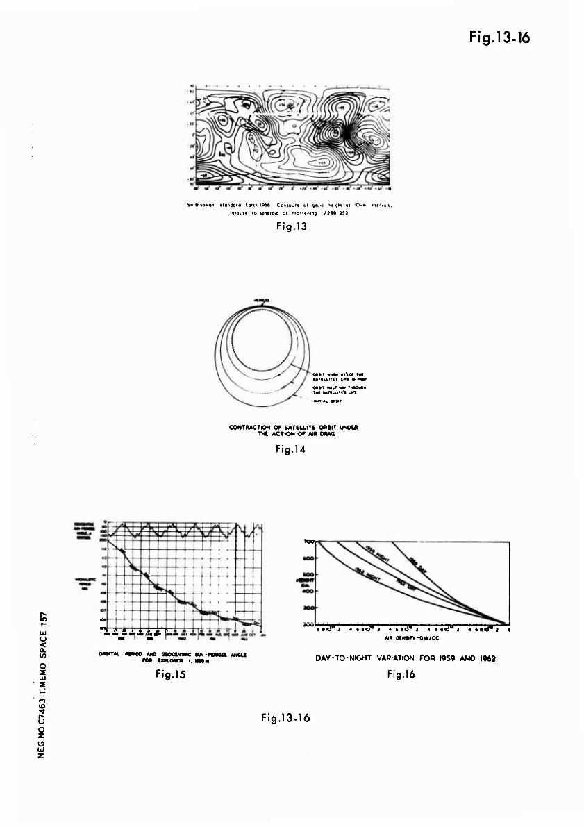
When a complete set of zonal, tesseral and sectorial harmonics has

been derived, it is convenient to summarize it in a contour map, representing

the height of the geoid (mean sea level) above a spheroid of some suitable

flattening. Fig.13 shows such a contour map based on the 1966 Smithsonian 2

Standard Earth ; it differs very little from the latest map for the 1969 9

Standard Earth .

4 THE UPPER ATMOSPHERE

The effects of the upper atmosphere on a satellite orbit are much more

difficult to represent, mathematically, than are the effects of the earth's

gravitational field. One reason for this is that the gravitational field

has a potential function - i.e. the field is conservative - whereas there

is no such function for the drag force exerted by the atmosphere. A more

important reason, however, is that the earth itself is essentially solid,

so that the harmonic coefficients, which specify the potential, are constant

(neglecting tides, earthquakes, etc.), whereas the atmosphere is changing all

the time. It is still possible to represent the perturbing force mathematically,

but the parameters of such a representation - for example the 'density scale

height' - can only be treated as constant in a first-order analysis of the

orbital perturbations.

In spite of the inherent complexity that we now have to face, the basic

expression for the aerodynamic drag force on a satellite is actually very

simple, viz.

D - - i p cD S V V , (11)

where p is the density of the air in the vicinity of the satellite, C

is the drag coefficient, V is the velocity of the satellite relative to

the surrounding air, and S is the projected cross-sectional area perpen-

dicular to the direction of V. For certain satellites there may also be

a lift force, but we ignore this possibility.

u

If the air is assumed to be stationary, relative to geocentric inertial

axes, so that V is identical with r, then D acts within the orbital

plane of the satellite and there is no tendency for the orbital plane to

rotate; i.e. with this assumption the motion becomes two-dimensional,

within a fixed orbital plane. (An actual orbital plane still rotates, of

course, due to gravitational perturbations, but, as I have said, the two

classes of perturbations may be considered as essentially independent.)

This two-dimensional motion is governed by the air density p, as it varies

along the orbit, and so information about p can be inferred by studying

the perturbations in the motion. I propose to give a brief survey of this

subject, and then to conclude with an even briefer survey of how

atmosphere-induced rotations of the orbital planes of various satellites

have been observed, with a surprising corollary about the rotational

speed of the atmosphere.

4.1 Air density

Equation (11) showed that the drag force is proportional to the air 12

density, and air density is primarily a function of height. Thus average —r "X

values of o are lü kg/m at about 100 km height, but less than -14 3

10 kg/m at 1000 km. The variation with height, h, is approximately

exponential, so that we have

h - h p ■ Po exp —g , (12)

where H is the 'density scale height* and p is the density at a

reference height h . To a first approximation H is taken as constant -

and would be about 50 km to reproduce the average variation from h ■ 100 km

to h - 1000 km that has been quoted - but if better accuracy is desired H

must itself be taken as a function of height.

Let us consider what happens to a satellite in an orbit of moderate

eccentricity, say for which 0.02 < e < 0.2. (It is the e > 0.02

part of the inequality which concerns us here.) It follows that the

effect of air drag is effectively concentrated within a small arc of the

orbit around perigee. Loss of energy near perigee means that the next

apogee is lower than the previous one, and the evolution of the orbit is

as shown in Fig.14. The orbit contracts and becomes more circular; i.e.

both a and e decrease with time. It is interesting to note the

slightly paradoxical fact that the height of perigee, where nearly all the

drag is, decreases only very slowly, whereas the height of apogee, where

there is virtually no drag, decreases relatively rapidly.

SP 157

SP 157

15

I capnot resist remarking on a further paradox which people sometimes

find difficult to understand: the immediate effect of drag is that a

satellite is retarded and its orbit contracts, but a contracted orbit means

(by Kepler's third law) a shorter orbital period, so that the satellite has

actually been accelerated. The paradox cannot be resolved by saying that a

contracted orbit means the satellite has less far to go; it really does

travel - on average - faster. The explanation, of course, is that a (genuine)

retardation at perigee involves a loss of energy and that it is at the next

apogee that - relative to the preceding one - a speeding up occurs. If, from

one apogee to the next, an amount of total energy AE has been lost, this

corresponds to a loss of potential energy amounting to 2 AE, so that there

is actually a gain of AE in kinetic energy.

It is the decreasing value of T, the orbital period, that is the most

easily and accurately measured perturbation of an orbit. The rate of change

of T is directly proportional to p , the reference density in

equation (12), so that from observations of t it is possible to infer p . 13 ^ o

The formula is

mi- 'a ' -0-157 f (Ä) i1 - 2e + 2^ - 8^ I1 - 10e + T& 4 0

(13)

where 6 - FSC./m; here F is a factor which can be introduced to allow for

atmospheric rotation and m is the mass of the satellite (which no longer

cancels out in the equations of motion, as it does for gravitational pertur-

bations). It is assumed, still, that 0.02 <e <0.2, and the formula is

derived by truncating asymptotic expansions of Bessel functions of argument

ae/H. The reference height, h , to which this value of p applies, is

not the height of the satellite's perigee, but a height JH above perigee.

The advantage of a formula which gives density at height h + JH is that

it is less sensitive to errors in H than a formula for density at height

h ; for example, an error of 25Z in H gives an error of only 1* in p.

(Since e is assumed to exceed 0.02, apogee height exceeds perigee height

by at least 250 km, so the air at height h + :lH really is being visited!)

The overall accuracy for absolute values of density, as given by equation (13),

is usually about 10Z, due to lack of an exact value for C . But variations

in density can be measured much more accurately, often to better than 2Z.

16 SP 157

Discoveries about the density of the upper atmosphere, based entirely

on the use of equation (13) for many satellites (in almost every case as a

'non-operational objective'), have been remarkable. The first discovery was

that the atmosphere was far less tenuous than had been supposed prior to the

satellite era. The second was that the density, at the same height above

the same point on the ground, can be incredibly different at one time from

another; at 500 km height, for example, the maximum value of p can be as

much as 200 times greater than the minimum value.

The variation of atmospheric density with time is under the control of

the sun, and this control acts in a number of ways, not all of which are

fully understood as yet. Some of the control mechanisms may be regarded as

acting 'directly', while others act 'indirectly', and an example of each of

these may be seen in the plot of T, for the satellite Explorer 1 (h about

350 km), in Fig.15. At heights between 200 km and 1000 km density increases

during the (local) morning, as a result of solar heating, and decreases

during the afternoon and evening, so that there is a 'day-to-night' varia-

tion which is 'indirect' in the sense that it is not associated with any

change in the sun itself. This effect does not manifest itself diurnally,

however, because the earth is rotating underneath the satellite orbit; it

is the angle between the sun and the satellite perigee, as seen from the

centre of the earth, which is important, and the period of a complete cycle

of variation of this angle is usually several months, about nine in the case

of Explorer 1. During each cycle the rate of decrease of T - and hence the

atmospheric density - is greater during the periods of perigee 'day' than

during the periods of perigee 'night'. The 'direct' effect in Fig.15 is

visible as the steady reduction in the rate of decrease of T from 1958 to

1962. This can only mean that the satellite perigee, as it very slowly

descended, sampled less and less dense air, contrary to what might be

expected. The explanation lies in the gradual reduction in solar activity

as the sun moved from the maximum of the 10- or 11-year sunspot cycle, in

1958, towards the minimum, in 1964. At heights above 200 km the atmospheric

density is directly related to the solar activity; as the extreme ultra-

violet radiation increases, and the particles ejected by the sun become

more numerous and more energetic, the air heats up and hence becomes denser.

The sunspot-cycle variation in density is greater than the day-to-night

variation, as can be seen from the four plots of density against height

shown in Fig.16.

SP 157

17

Besides the correlation with the sunspot cycle, the direct response

of the atmosphere to solar activity shows itself in two other ways, both

of which may be seen in the plot of f for Explorer 9 (h about 700 km)

in Fig.17. The peaks in this plot correspond to violent storms on the sun,

alternative evidence for which is given by the geomagnetic index a ,

which is probably the best indicator of the effect of solar particles

impinging on the earth and is also plotted in Fig.17; the correlation

between a and f is very striking. (Similar striking correlations

between f, for various satellites, and the energy of solar radiation at

wavelength 107 mm have been observed.) If we ignore the peaks, the other

feature of the T plot in Fig.17 becomes clear, namely the 27-day cycle.

A cycle of this period is characteristic of solar phenomena, since it is

the period of the sun's rotation.

Finally, in this summary of solar-induced variations in the density

of the upper atmosphere, there is the 'indirect* effect known as 'semi-

annual variation'. Though the effect is believed to arise from variations 14

in the lower atmosphere , it is most clearly visible high in the upper

atmosphere. Fig.18 shows the effect for Echo 2 (h about 1100 km>, The

cause of the semi-annual variation is still uncertain, but its features

are well established: the density at a given height, after correction for

all other sources of variation, exhibits a residual oscillation which has

maxima in early April and late October and minima in mid-January and

late July; the maximum in October is usually - though not in Fig.18 -

higher than that in April, and the minimum in July is usually lower than

that in January.

4.2 Atmospheric rotation

I" have already remarked that, if it were not for the rotation of the

atmosphere (and for the possibility of lift forces), there would be no

tendency for atmospheric forces to rotate the orbital plane of a satellite.

Thus if any slight rotation of an orbital plane is observed, after correc-

tion for non-atmospheric perturbations, it will provide direct evidence -

not merely that the atmosphere rotates, which is obvious - but of the

magnitude of the rotation.

Suppose, then, that the atmosphere has an angular velocity which is A

times greater than that of the earth itself. Here A may be assumed to be

a function of height, equal to 1.0 when h « 0; we might suppose that as h

increases A would decrease, since the frictional effect of the earth would

wear off, but this turns out to be wrong.

1R SP 157

Fig.19 gives a vector diagram for velocities and drag forces as a

typical satellite crosses the equator from south to north. By resolving

the drag force D within and perpendicular to the orbital plane, it is

seen that there is a small lateral force which tends to decrease the

inclination of the orbit. Half an orbit later, as the satellite crosses

the equator from north to south, the force acts in the opposite direction,

but this means that its tendency is still to decrease the inclination.

In fact TT ^ 0 all round the orbit, except at the north and south apexes

where TT " 0 (and except for an equatorial orbit, for which JT " 0

everywhere) . The integrated effect around an orbit can be expressed, like

the ordinary atmospheric perturbations, in terms of Bessel functions; the

resulting change in the inclination, Ai say, contains p (the density

at height h + iH) as a factor, and p can then be expressed in terms

of T, by equation (13). The final formula is best expressed in terms 13

of AT, the change in T over a long interval of time, and it is given by

Ai A AT sin i

3 /F (1 - 4e) cos2 ai - ^- cos 2a) + 0 |e% ~^]} . CM) • (•'• AI ■

Thus if Ai is observed, for a suitable satellite for which an appreciable

AT has also been observed, a value for A can be estimated. (Formulae for

Af; and Au can also be obtained, but are of less practical use.)

Values of A for 27 satellites are shown in Fig.20 with the extra-

ordinary indication that A increases with height. The standard deviation

of each determination of A is large, due to the smallness of the values of

Ai used, but the effect must be regarded as a genuine one, and it has been

confirmed more recently for other satellites . As an example of the care

which has to be exercised, however, I can point to the Ariel 3 tesseral-

harmonic resonance I described earlier; if this were overlooked, it would

be possible to obtain a value for A of about 2.3, taking a Ai of about

-0.018 over two years from Fig.11, but when the resonant effect is allowed

for the value obtained for A seems to be less than 1.

A number of attempts have been made to explain the observed increase

of A with height. Challinor's model of ionospheric winds, for example,

leads to A = 1.1 at 200 km, rising to nearly 1.5 at 350 km, and this is in

excellent agreement with Fig.20.

Acknowledgement

I am grateful to D. G. King-Hele for allowing me to use a number of

illustrations from his publications.

SP 157

No. Author(s)

1 R. H. Merson

10

C. A. Lundquist

G. Veis

D. G. King-Hele

G. E. Cook

D. E. Smith

Y. Kozai

D. G. King-Hele

G. E. Cook

Diana W. Scott

Y. Hagihara

R. R. Allan

E. M. Gaposchkin

K. Lambeck

R. R. Allan

19

REFERENCES

Title, etc.

A brief survey of satellite orbit determination.

RAE Technical Report 66369 (1966)

Phil. Trans. Roy. Soc, A, 262 (1124), p.71 (1967)

Geodetic parameters for a 1966 Smithsonian

Institution Standard Earth.

Smiths. Astr. Obs. Sp. Report 200 (1966)

The even zonal harmonics of the Earth's gravita-

tional potential.


Geophys. J., 10, p.17 (1965)

A determination of the even harmonics in the

Earth's gravitational potential function.

Planet. Space Sei., 13, p.1151 (1965)

Revised values for coefficients of zonal spherical

harmonics in the geopotential.


Evaluation of odd zonal harmonics in the geo-

potential, of degree less than 33, from the analysis

of 22 satellite orbits.



Recommendations on notation of the earth potential.

Astron. J., 67, (1), p.108 (1962)

Resonance effects due to the longitude dependence

of the gravitational field of a rotating primary.



1969 Smithsonian Standard Earth (II).


On the motion of nearly synchronous satellites.


Proc. Royal Soc, A, 288, p.60 (1965)

20 SP 157

No.

11

12

13

14

15

16

Author(s)

R. H. Gooding

D. G. King-Hele

D. G. King-Hele

G. E. Cook

D. G. King-Hele

Diana W. Scott

Doreen M.C. Walker

R. A. Challinor

REFERENCES (Contd)

Title, etc.

The orbit of Ariel 3 (1967-42A).


The upper atmosphere and its Influence on

satellite orbits.


Dynamics of Satellite«! 1969 (ed. B. Morando),

p.249, Springer Verlag, Berlin (1970)

Theory of satellite orbits in an atmosphere.

Butterworths, London (1964)

The semi-annual variation in the upper atmosphere:

a review.


Annales de G^ophysique, 25, p.451 (1969)

Upper-atmosphere rotational speed and its varia-

tion with height.



Neutral-air winds in the ionospheric F-region

for an asymmetric global pressure pattern.

Planet. Space Sei., 17, p.1097 (1969) and 18,

p.1485 (1970)

Fig.1-6

EXISTING ORBITAL MODEL

INDIVIDUAL OBBIT DETERMINATIONS

OPUuaiOHH. OtJKTIVtt

ORIIT ACHICVtMCNT

CüIMNCC AND CONTROL

ON-MMO INSTKUMCNTkriON

TRACKING / TILCMCTHY SCHCOULINC

NOW-ORWATIONAL OMKTIVtS

GENERAL SURVEILLANCE

SENSOR ACCURACY

NAVIGATION AND GEOOEiT

EARTHS GRAVITY FIELD

AIR DENSITY/ROTATION

^^ i r i ■

GRAPH OF AN ORBITAL PARAMETER

IMPROVED EARTH CONSTANTS

IMPROVED MODEL

Fig.l Fig.2

FLATTDHNC OF THE CARTH (CMCATLV CXAOGCMTCO) THE FLATTCMNG f MAY K

OCWNCO At f« 0,-Dp

Fig.3

'.) »•<•

(0 •"• («) ••»

FO«M Of THE 2NO-STH HARMONICS (NOT TO »CALt)

Fig.4

in

Lü u < Q. in

ui

u o z 6 z

Talii— of m|

*,,thM•, Ae«ek(l9<9) (19«5) 0969)

106J,

ieV

10'JX

10'J,

10*J,

106J,

106J,

10

12

14

10oJ K

10oJ

1C6J

18

20

1082.(4 1082.64 1082.6)

-1.52 -1.70 -1.59

0.57 0.7J o.so

0.44 -0.46 •0.12

-0.17 -0.J5

■0.22 ■0.04

0.19 -0.07

0.19

-0.2J

•0.01

Fig.5

OABIT AT A LATER DATE

ORBIT SWINGS WESTWARDS ''*

«WIT OF SATELLITE

THE EFFECT OF THE EARTH'S EQUATORIAL

BULGE ON A SATELLITE ORBIT

F.g.6

Fig.1-6

Fig.7-12

Vilu«» of oii toatl bimonlc» ('969)

'cV -2.54 -?.V

'f% -o.?i -0.^3

«c^. -0.40 -0.36

.c% 0 -0.10

'C^,, 0 0.20

'A3 0 -0.12

'c6.,. -o.?o -0.17

-c^,, c 0.08

^\ 0 -0.??

,0%, 0.?6 0.15

•=%, -0.15

JJJ,J?VJ29,J31 0

Fig.7

-rW MOO« MWMM*

eCCCNTRlCITV OF ARI€L 3 -NASA AND R»£ VALUES COMPARED

Fig.8

MEICHT Of TMf CIOIO DILATIVI TO * SPMIDOIO Of fL»tTINIMC ''»»• as, *s civCN tv T-cotfficiCNi «i or »uo IONAL HARUONICS

Fig.9

O DAY I x DAY 2 □ DAY 5 + DAY 4

Fig.10

!l ' (

•aw«/: 0

"•.. r.. V-"1?»

Fig.11

Fig.7-12

«00.| ,.''■

s.\ ^

■6".i \

■O'i» \,. , f / 'v;,'

TIC?

140*

* IftO*

■ •o"

1*' l«M 19«* ' AM u ItM

w»oo

ORBITAL INCLINATION AND RESONANT

VARIABLE FOR ARIEL 3 (l967-4aA)

Fig.12

in

UJ u < OL

UJ

CM (O

o d z d

Flg.13-16

SffniMonign Hondo cd Egrth 1966 Contour o' q*u<d i^t iqht ol lO-ic inter «of» ■

rtiolivt to »phtrod of tloiitrtmq l/298 2S3

Fig.13

OMIT WHtM llXCW tMt UfliLitri UM « M»T

oatrr MAL« ■** TiMputii TM unu.iri'1 L*a

CONTRACTION Of SATELLITE OftBIT ÜNDW THC ACTION OF AIR DRAG

Fig.14

u

to

UJ

"• i» « il » »li i 4l MMF «« Hd UMIJM iPV M

im I rnt

OMITM. «moo AND moooimc m> nwuMn i.

«M-WMtt «MGU

Fig.15

VBO

* tid" i 4 »iid" t 4 t lid" i 4 » nd" a 4 »i^" a 4 MR 0INtlTV-CM7CC

DAY-TO-NIGHT VARIATION FOR 1959 AND 1962.

Fig.16

D o z UJ

Fig.13-16

ig.17.20

-] 1 111 1 M 1 Mi 1 1 1 ' "• '* ' M 1U HmHJ^^' yi^n Iwwwa'cMii 1 :

11 i j XJJiLJidJvJk.iAJ.fiaLLJ

txnpKt*». * HO SfOutMenc rncti v

Fig.17

Air «entity in IM4-S at • Mifht of MM ha. Puio. fr*fll t**»0 a ■ 0*Ur corrtctian tor tetor octivilr

Fig.18

V- Vtioc'tf ffiat.*t to EcrtM CCM'«

V ' VflQCtly rfiotivc to Qir

K.ncmcit'CS of spherical c>aWltilc S .n a c^rcylor ofbit 04

it croi«> thrf equator

-i 1 1 1 1 1 1 1 1 r

Fig.19 Fig.20

in

u u < Q.

i

Flg.17.20 u d z; o

R. H. Gooding November 1970 - dtic.mil · ROYAL AIRCRAFT ESTABLISHMENT Technical Memorandum Space...

Documents

Transcript of R. H. Gooding November 1970 - dtic.mil · ROYAL AIRCRAFT ESTABLISHMENT Technical Memorandum Space...