q%(x) 2-;/2q(2-;x- L2(E).

SIAM J. MATH. ANAL.Vol. 24, No. 2, pp. 499-519, March 1993

1993 Society for Industrial and Applied Mathematics014

ORTHONORMAL BASES OF COMPACTLY SUPPORTED WAVELETSII. VARIATIONS ON A THEME*

INGRID DAUBECHIES

Abstract. Several variations are given on the construction of orthonormal bases ofwavelets with compactsupport. They have, respectively, more symmetry, more regularity, or more vanishing moments for the scalingfunction than the examples constructed in Daubechies [Comm. Pure Appl. Math., 41 (1988), pp. 909-996].

Key words, wavelets, orthonormal bases, regularity, symmetry

AMS(MOS) subject classifications. 26A16, 26A18, 26A27, 39B12

1. Introduction. This paper concerns the construction of orthonormal bases ofwavelets, i.e., orthonormal bases {$jk; j, kZ} for L2(R), where

(1.1) q%(x) 2-;/2q(2-;x- k)

for some (very particular!) L2(E). The functions (1.1) are wavelets because theyare all generated from one single function by dilations and translations. Note thatwavelets need not be orthogonal or even linearly independent. In fact, the "first"wavelets were neither [1], [2]. See [3], [4] for discussions of wavelet expansions usingnonindependent wavelets, with continuous [3] or discrete [4] dilation and translationlabels. Even the special case of orthonormal wavelets need not always be of the form(1.1). Basic dilation factors different from 2 are possible: there exist orthonormal basesin which this factor is any rational p/q > 1 [5]; in more than one dimension we mayeven choose a dilation matrix instead of an isotropic dilation factor. In these moregeneral cases, it may be necessary to introduce more than one (but always a finitenumber). We shall restrict ourselves to one dimension here, and to the dilation factor2, as in (1.1). Bases with factor 2 are by far the easiest to implement for numericalcomputations.

All interesting examples of orthonormal wavelet bases can be constructed viamultiresolution analysis. This is a framework developed by Mallat [6] and Meyer [7],in which the wavelet coefficients (f, Ojk) for fixed j describe the difference between twoapproximations of f, one with resolution 2j-, and one with the coarser resolution 2.The following succinct review of multiresolution analysis suffices for the understandingof this paper; for more details, examples, and proofs we refer the reader to [6] and [7].

The successive approximation spaces V in a multiresolution analysis can becharacterized by means of a scaling function ok. More precisely, we assume that theinteger translates of b are an orthonormal basis for the space Vo, which we define tobe the approximation space with resolution 1. The approximation spaces V withresolution 2 are then defined as the closed linear spans of the bk (k 7/), where

(1.2) dpjk 2-J/adp(2-Jx- k).

To ensure that projections on the V describe successive approximations, we requireVo c V_l, which implies

(1.3)

* Received by the editors May 29, 1990; accepted for publication (in revised form) May 23, 1992.? Mathematics Department, Rutgers University, New Brunswick, New Jersey 08903 and AT&T Bell

Laboratories, 600 Mountain Avenue, Murray Hill, New Jersey 07974.

499

500 INGRID DAUBECHIES

This imposes a restriction on b: since b Vo c V_l=Span{b_lk; k7/}, there mustexist c. such that

(1.4) (x) c,, (2x n).

In order to have a complete description of L2(), we also impose

(1.5) fq V {0}, U L().jZ jZ

For every multiresolution analysis as described above, there exists a correspondingohonormal basis of wavelets defined by

(1.6) (x) Z (-1)"c_,+6(2x- n),

where c, are the coefficients in (1.4). We can prove [6], [7] (see also below) that the4o, are then an orthonormal basis for the orthogonal complement Wo of Vo in V_I.This phenomenon repeats itself at every resolution level j. It follows that, for every j,the (f, qgk) determine the difference in information between the approximations PfP-lf at resolutions 2j, 2j-, respectively:

Pj-lf-- Pf+E (f, q’jk)qgk.

Consequently, by (1.3) and (1.5), the (jk’ j, k 7/) constitute an orthonormal basis for().

One advantage of the "nested" structure of a multiresolution analysis is that itleads to an efficient tree-structured algorithm for the decomposition and reconstructionof functions (given either in continuous or sampled form). Instead of computing allthe inner products (f, ltjk directly, we proceed in a hierarchic way:

mcompute (f, (jk) for the finest resolution level j wanted (if the data are givenin a discrete fashion, then these discrete data can just be taken to be (f

--then compute (f q-k) and (f b-k) at the next finest resolution level byapplying (1.4) and (1.7),

1(f, qg-,k) , (-- 1)"C-,,+2k+l(f 6j,,),

--iterate until the coarsest desired resolution level is attained.The total complexity of this calculation is lower, despite the computation of the

seemingly unnecessary (f, b2k), than if the (f, q%) were computed directly.This brief review shows how to construct an orthonormal basis of wavelets from

any "decent" function b satisfying an equation of type (1.4). An example of such aconstruction is given by the Battle-Lemari6 wavelets, consisting of spline functions[8], [9], [10]. In general, constructions starting from a choice of 4 lead to 4, q, whichare not compactly supported (see, e.g., [15], [25] for a more detailed discussion). Theconstruction can, however, also be viewed differently. The Fourier transform of (1.4)is

which implies

(1.7) (s:) [= mo(2-Jsc)] (0),

ORTHONORMAL BASES OF COMPACTLY SUPPORTED WAVELETS II 501

with mo()= 1/2 . c,, e i", so that, up to normalization, b is completely determined bythe c.. Fixing the c., therefore, also defines a multiresolution analysis. The c. have tosatisfy certain conditions. Combining (bok, 4o)= 6k with (1.4) immediately leads to

(1.8) C,,C.-2k 26k0,

where we have assumed, as we shall do in the sequel, that the c. are real. In terms oftoo(sO), (1.8) can be rewritten as

(1.9) Imo()l+ Imo(:+ r)l2= 1.

To ensure that b is well defined, the infinite product in (1.7) must converge, whichimplies too(0)-- 1 or

(1.10) c=2.

It follows that 4 is uniquely determined by (1.4), up to normalization, which we fixby requiring dx 4(x)= 1. One can show (see, e.g., [12]) that (1.9) implies that b isin L-(), but unfortunately (1.8) is not sufficient to guarantee orthonormality of thebo,. A counterexample is Co=C3 1, all other c,-0, which leads to b(x)=] for0 <- x < 3, 4(x) 0 otherwise. Such counterexamples are rare, however. If N N 3,then the example above, o 3 1, is the only one. For a detailed discussion, see 12],13], [22].

If we exclude these thin sets of "bad" choices for the c (which can be done byvarious means [6], [7], [12] [13], [15]), then we can build orthonormal bases ofwavelets starting from the c,. Once orthonormality of the bOk is established, all therest follows easily. Formula (1.6) for q leads immediately to orthogonality of the qOland 4Ok,

1(_l).c_.++,c,._(_,.

1

2(-1) c_++c,_ 0.

The last equality follows from the substitution n m + 2(k + l) + 1 for the summationindex n. Similar manipulations prove

and

(1.11)k

It follows that both {b-1,; n ;7} and {(0k, 0k; k Z} are orthonormal bases for V_I.(In other words, (1.8) ensures that (1.4) and (1.6) describe an orthonormal basistransformation.) It follows that Wo Span (qOk) is the orthogonal complement of V0in V_, and hence that the {qgk; J, k 7/} constitute an orthonormal basis for L2(R).

Constructing q from the c, rather than from b has the advantage of allowingbetter control over the supports of b and q. If c, 0 for n < N1, n > N2, then support(b)c [N, N2] (see [lla], [14]). In [15] this method was used to construct orthonormalbases of wavelets with compact support, and arbitrarily high preassigned regularity(the size of the support increases linearly with the number of continuous derivatives).These orthonormal basis functions and the associated multiresolution analysis have


been tried out for several applications, ranging from image processing to numericalanalysis [16]. For some of these applications, variations on the scheme of [15] wererequested, emphasizing other properties. The goal of this and the next paper is topresent a number of these variations.

The construction in [15] relied on the identity

s (N--l+J)[(cosoz)2rV(sina)2J+(sina)2(cosa)2] 1.(1.12)j=O j

Since

(1.12) suggests the choice

(1 13) mo()=(l+ei)1

2Q(e’)’

where Q is a trigonometric polynomial with real coefficients such that

(1.14) IQ(e’)l--- j=o j 2

By (1.12), any such mo will satisfy (1.9). To determine 0, we have to extract the "squareroot" of the right-hand side of (1.5). This can be done by using a lemma of Riesz [17].Denote the right-hand side of (1.14) by Pc(ei), and extend PN to all of C. We havePN(Z)--PN() and Pc(z-1) PN(Z). Consequently, the zeros of Pn come either inreal duplets, rk and r{ or in complex quadruplets, Zl l, z-f and -P(z) =4-

\ N- 1 ]z- (z- rk)(Z-- r; 1)

[I (Z-- Zl)(Z- l)(Z-- Z;1)(Z- ;1)

=4- \N-1].U

(Z ZI)(Z l)(Z, Z-1)(/-- Z-1)

It follows that PN(e’) [Q(e’t)[, with

(1.15) Q(z)=2-N+I(2N-211/2N-l/ (z-r,) (zZ+lz, lZ-2Zlz, Re z,)

This gives a recipe for the construction of mo:(1) For given N, determine the zeros of PN;(2) Choose one zero out of every pair of real zeros r, r[ of PN, and one conjugated

pair out of every quadruplet Zk, Z-(3) Compute the product Q, and substitute into (1.12).The result is a polynomial in e of degree 2N 1, corresponding to an orthonormal

basis of wavelets in which the basic wavelet has support width 2N-1. Since (1.6)can be rewritten as

0(l) ei((/-)+)mo + "rr


and since (1.13) has a zero of order N at 7r, it follows that qN has N vanishing moments,

dxxld/N(X) =0, =0, 1,..., N- 1,

which is useful for quantum field theory [18] and numerical analysis applications [19].The regularity of the PN constructed in 15] increases linearly with their support width,qN Ca(N), with limu_ N-la(N) .2075 [23], [24], [25]. Plots of and q for variousvalues of N can be found in [15], [25].

Depending on the application they had in mind, several scientists (mathematiciansor engineers) have requested possible variations on the construction in [15]. Thefollowing are the most recurrent wish items.

(1) More symmetry: the functions , 0 in [15] are very asymmetric. Completesymmetry is incompatible with the orthonormal basis condition (see [15, p. 971], or2 below), but is less asymmetry possible?

(2) Better frequency resolution" orthonormal bases with basic multiplication factor2 correspond to frequency intervals of 1 octave. Is better possible (e.g., 1/2 octave),without giving up compact support?

(3) More regularity: is better regularity than in [15] achievable for the samesupport width ?

(4) More vanishing moments: for a fixed support width 2N-1, the PN of [15]have the maximum number of vanishing moments. The functions eu do not satisfyany moment condition, except dx eN(X)= 1. For numerical analysis applications, itmay be useful to give up some zero moments of 0 in order to obtain zero momentsfor , i.e., to have

dx&(x) 1,

(1.16) I dx xlch(x) O, 1,..., L,

dxxl(x) =0, l=0,..., L.

How can such , be constructed? They would have the advantage that inner productswith smooth functions are particularly appealing:

f dx b-jk(x)f(x)-- 2J/2 f dx qb(2J(x-2-Jk))f(x)

2-J/f(2-Yk) + correction terms in f+l(use the Taylor expansion off around 2-2k; the second through (L+ 1)th terms vanishbecause of (1.16)). Moreover, if the (L+ 1)th derivative of f is uniformly bounded,then the correction terms in this formula are of order 2 -(/’+l/2)j.

The purpose of this and the next paper is to show how such variations can be,constructed. In 2 we handle symmetry, in 3 regularity, and in 4 vanishing momentsfor . The next paper shows how to obtain better frequency localization.

2. More symmetry. If we restrict our attention to orthonormal bases of compactlysupported wavelets only, then it is impossible to obtain which is either symmetric orantisymmetric, except for the trivial Haar case (Co 1, Cl =-l, all other c, =0). Thisis the content of the following theorem.


THEOREM 2.1. Let b, dp be defined as in 1, from a finite set of coefficients c,satisfying (1.9) and (1.11 ), with orthonormalo. If is either symmetric or antisymmetricaround some axis, then is the Haar function.

A proof can be found in [25, Chap. 8].It is thus a fact of life that symmetric or antisymmetric , however desirable they

might be in applications, are just not possible within a framework of orthonormalbases of continuous, compactly supported wavelets. On the other hand, b and q donot really need to be quite as asymmetric as in [15], where the extreme asymmetry ofq, proceeds from choices made in their construction. In practice, the 2(N- 1) zerosof PN consist of one real pair r, r- and n quadruplets of complex zeros ZI, 1, Z-1

)-1 if N--2no is even, and of no quadruplets if N 2no+ 1 is odd. To construct QN,we need to select one of the two real zeros, and one pair Zl, out of every quadruplet.The choice made in 15] is the so-called extremalphase choice: we chose systematicallyall zeros with modulus smaller than one. Other choices may lead to less asymmetric. The following argument shows why.

A sequence of real numbers (a,) is said to define a linear phase filter if thephase of the function a(sc) a ei is a linear function of :, i.e., if, for some ;g/2,

This means that the a, are symmetric around l, a,- Ol21_ If the sequence does notdefine a linear phase filter, then the deviation from linearity of the phase of c(:)reflects the asymmetry of the a,. The Fourier transform of is given by the infiniteproduct (1.7). If c, were symmetric around l, then we would have mo(:)- eilelmo()l,hence

(:) =exp il 2-: Imo(2-)11(o)1j=l j=

so that would be symmetric around as well. As explained above, this is impossiblefor c, satisfying (1.8). The closer the phase of mo is to linear phase, the closer thephase of th will be to linear phase, and the less asymmetric b will be. In our case, mois a product of factors of type

(2.1)z Zl)( z 1 e it ei R1 ei,)( 1 e-u:Rl e-’’)

ei[ei-2Rl cos al+ Ri e-ie],

with possibly an extra factor

(2.2) (a- r) eiU2[eiU2- r eiU2].

The total phase of mo is a sum of the phase contributions of each factor. Apart fromlinear phase terms, the phase contributions of (2.1) and (2.2) are, respectively,

( (1- R) sin sc )(2.3) O(:)=arctg (l+R)cos-2RlCOSCll+r

(2.4) arctg\l-r tg).

The valuation of arctg should be chosen so that (I) is continuous in [0,27r], andql(0) =0. Since the denominator in (2.3) has two zeros, namely,

2RI )Arc cos l+RCS


and 2w :, 1(27r) /(0) + e27r, with e + 1. Something similar happens in the(z-r) case. In order to extract only the nonlinear part of t, we define, therefore,

( (1- R) sin sc ) sc (27r)/(:) arctg(1 + R) cos :-2R cos al

or

l+rarctg i r

,I’,(2rr).

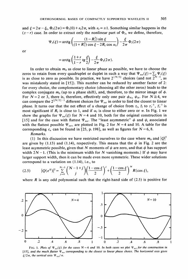
In order to obtain mo as close to linear phase as possible, we have to choose thezeros to retain from every quadruplet or duplet in such a way that ,o,(:)=Y ()is as close to zero as possible. In practice, we have 2 tN/2j choices (and not 2N-i, aswas mistakenly stated in [15]). This number can be reduced by another factor of 2:for every choice, the complementary choice (choosing all the other zeros) leads to thecomplex conjugate mo (up to a phase shift), and, therefore, to the mirror image of b.For N 2 or 3, there is, therefore, effectively only one pair N, i]/N" For N >-4, wecan compare the 2 [S/2J-1 different choices for o, in order to find the closest to linearphase. It turns our that the net effect of a change of choice from zt, to z-1, -i ismost significant if RI is close to 1, and if at is close to either zero or 7r. In Fig. 1 weshow the graphs for ot() for N =4 and 10, both for the original construction in[15] and for the case with flattest tot. The "least asymmetric" b and q, associatedwith the flattest possible ,ot, are plotted in Fig. 2 for N =4 and 10. A table for thecorresponding c, can be found in [25, p. 198], as well as figures for N 6, 8.

Remarks.(1) In this discussion we have restricted ourselves to the case where mo and QI2

are given by (1.13) and (1.14), respectively. This means that the b in Fig. 2 are theleast asymmetric possible, given that N moments of q are zero, and that b has supportwidth 2N-1. (This is the minimum width for N vanishing moments.) If b may havelarger support width, then it can be made even more symmetric. These wider solutionscorrespond to a variation on (1.14), i.e., to

(2.5) IQ(e’e)[2= + R(cos sc)=o j 2 2

where R is any odd polynomial such that the right-hand side of (2.5) is positive for

.2.5

0 0

--.5--.2

-1

N=IO

FiG. 1. Plots of ,o,() for the cases N =4 and 10. In both cases we plot ,o, for the construction in

15], and the much flatter q,o, corresponding to the closest to linear phase choice. The horizontal axis gives

7r, the vertical axis

0 .2 .4 .6 .8 0 .2 .4 .6 ..8


1.5

-.52 4 6

-1

-2

2

I//4

-2 0 2

1.5

-.5 I0 5 10 15

I,-5 0 5

FIG. 2. Plots of bv, bN closest to linear phase, for the cases N =4 and 10. In every case, support(bN) [0, 2N- 1], support (rv) [-N + 1, N].

all sc. The functions 4) constructed in {} 4, for instance, are more symmetric than thosein Fig. 2, but they have large support width

(2) We can achieve even more symmetry by going a little beyond the multiresol-ution scheme explained in 1, and by "mirroring" the filters at every odd step. Formore details, see [25, p. 256].

(3) In [21] the construction of orthonormal bases of wavelets is genera.lized to"biorthogonal bases," i.e., to two dual unconditional bases { {ljk; j, k 7/} and { Illjk; j, k7/}. The construction in [21] corresponds to a decomposition+reconstruction schemein which the reconstruction filters differ from the decomposition filters. In this moregeneral framework, complete symmetry can be achieved. Orthonormality is then lost,however, which is less desirable for some applications.

3. More regularity. The regularity of the wavelets g,, constructed in 15] increaseslinearly with their support width, 0N C(N), lim N-la(N)=.2075. The techniqueused in [15] to control the regularity of bN, $N involved constructing mo(:) so thatit contained the factor 1/2(1 + ei) with as high multiplicity as possible,

(3 1) mo()=(N

\ 2

where QN is a polynomial in ei oforder N- 1 (see I). Since l-I=o (I + exp (i2-sc))/2eie(sin so/so), we find (use (1.7))

N() e’Ne/2[sin so/2" N

s/2 II Q,,, (2-).


T,ogether with control on the infinite product of QN (see [15]), this leads to decay forthN as I:[ - c, hence to regularity for bs, N.

In this argument, imposing high order divisibility of mo by 1/2(1 + e i) is used as atechnical tool to obtain regularity. On the other hand, regularity for b implies that mois of type (3.1). More precisely, if b is compactly supported and th C L, then mo mustbe divisible by [1/2(1 + ei)]L; see [22], [21]. Since bN C’N for large N, with /z-.2,this means that at least 1/2 of the factors (1 + e) in mo,N are necessary. Can the othersbe dispensed with, allowing even shorter support for the same regularity, or higherregularity for the same support width? The answer is yes.

In [1 lb], an alternative way was used to determine the regularity of functions bsatisfying an equation of type (1.4). Unlike the methods in [15], the method of [llb]does not use the Fourier transform. Instead, two N-dimensional matrices To, T aredefined, To)d ce__, T). c_, 1 <= i, j <= N, where we assume c, 0 for n < 0or n > N. Divisibility of m0 by (1 + ei) with multiplicity L is equivalent to

N

(3.2) c,,(-1)"n 1=0, /=0,...,L-1.n=0

In terms of the matrices To, T1, this implies that there exists a flag of subspacesU1 c... c Ut of u, with dim U =j, such that

U is left-invariant under both To, T1.The left restrictions of To, T to U have the j eigenvalues 1, 1/2,..., 2 -j+l.

Let V be the subspace for N orthogonal to UL; V is right invariant for To, T.If, for some A < 1, C > 0, and for all rn

(3.3) Td,’’" Tdmlv,ll--<-- CA"2-"-’) (dj 1 or 0),

then (3.2) implies that b C L, and that its Lth derivative bt) is H61der continuouswith exponent ]log2 AI; if )t is best possible in (3.3), then [log2 A[ is the best possibleH61der exponent for bL). In principle (3.3) involves infinitely many inequalities; inpractice we substitute finitely many conditions sufficient to ensure that (3.3) holds forall m [llb, Prop. 3.11]. The value of b and its derivatives at any point x in support(4’) is governed by the behavior of the infinite product Td,(x)Ta)" Td,(x)..., whered(x) are the digits in the binary expansion of x, x Ix] + Y=I d(x)2-. Special, "local"inequalities of type (3.3), valid only for certain sequences (d),, can, therefore, betranslated into local regularity estimates, leading, in many examples, to a hierarchy offractal sets corresponding to different local H61der exponents. For more details, see[llb].

This approach can be used to study the regularity of compactly supported basiswavelets, which all correspond to an equation of type (1.4) with finitely manycoefficients. For the examples of [15], this analysis was carried out in [11b] forN 2, 3, 4 (for higher N, checking (3.3) becomes very complicated). In these threecases, the best possible H/Slder exponent for the highest order well-defined derivativeof bN was determined; these results were significantly better than what had beenobtained in [15] via Fourier analysis. Table 1 compares the regularity results of [15]and 1 lb].

The optimal estimates obtained in [11] illustrate again that some of the factors(1 + ei) of mo, or, equivalently, some of the sum rules (3.2), which we impose in orderto obtain regularity, are "wasted" in the final construction. N sum rules can deliverup to N-1 continuous derivatives if everything else cooperates; because of the otherconstraints on the cn (i.e., (1.8)), wavelets do not achieve this optimal number. Wecan, therefore, drop some of the sum rules, and use the additional degrees offreedom


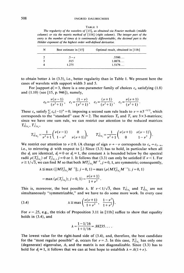
TABLEThe regularity of the wavelets of [15], as obtained via Fourier methods (middle

column) or via the matrix method of b] (right column). The integer part of theentry is the number of times ck is continuously differentiable; the decimal part is theH6Ider exponent of the highest order well-defined derivative.

N Best estimate in [15] Optimal result, obtained in [1 b]

2 .5 e .5500...3 .915 1.0878...4 1.275 1.5179...

to obtain better A in (3.3), i.e., better regularity than in Table 1. We present here thecases of wavelets with support width 3 and 5.

For Isupport b 3, there is a one-parameter family of choices cn satisfying (1.8)and (1.10) (see [15, p. 946]), namely,

u(u- 1) (1- u) (u+ 1) u(u+ 1)Co= (v2+ 1) Cl--(/,2-{ 1)’ c2=(v+ 1)’ c3= (v+ 1)

These cn satisfy c,(-1)" =0; imposing a second sum rule leads to v +3 -/2, whichcorresponds to the "standard" case N 2. The matrices To and T are 3 3-matrices;since we have one sum rule, we can restrict our attention to the reduced matrices

1 (v(v-1) 0 ) TI] 1 (v(v+l) v(v-1))TOlVl-v+l 1-v2 v(v+l) v, v2+l 0 1-v2

We restrict our attention to v-> 0. (A change of sign v-v corresponds to c,- c3_,

i.e., to mirroring b with respect to .) Since (3.3) has to hold, in particular when allthe d are identical, d-= 0 or d- 1, the constant Z is bounded below by the spectralradii p(T[v,) of Tlv,, j 0 or 1. It follows that (3.3) can only be satisfied if v<l. For

M-v -> 1/x/, we can find M so that both MTIv, ,j 0, 1, are symmetric; consequently,

A_<max (]]MT]v,M-11]; j--O, 1) max (p(mTjlvm-1); j--0, 1)

=max (p(Tlv,)" j=0, 1)=v(v+ 1)1+/,2

This is, moreover, the best possible h. If v<l/x/, then Tolv, and Tl[v, are notsimultaneously "symmetrizable," and we have to do some more work. In every case

(3.4) A_-->maxl+v2 1+

For v=.25, e.g., the tricks of Proposition 3.11 in [llb] suffice to show that equalityholds in (3.4), and

1-1/16A .88235

1+1/16

The lowest value for the right-hand side of (3.4), and, therefore, the best candidatefor the "most regular possible" b, occurs for v=.5. In this case, T1]v, has only one(degenerate) eigenvalue, .6, and the matrix is not diagonalizable. Since (3.3) has tohold for dj 1, it follows that we can at best hope to establish A .6(1 + e).


In fact, we cannot achieve even this much. It turns out that [p(To, T12)] 1/13.659676... >.6, meaning that we can certainly not hope for a smaller h than .659..-.Using all the tricks in Proposition 3.11 in 1 lb], and checking a collection of buildingblocks with up to 17 factors, we find h <= .666. More work leads to smaller upper boundsfor A; presumably the best value is the .659 obtained above.

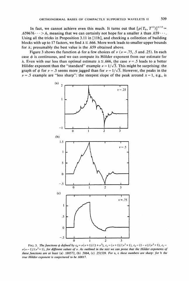
Figure 3 shows the function 4’ for a few choices of u (, .75, .5 and .25). In eachcase 4, is continuous, and we can compute its H61der exponent from our estimate forA. Even with our less than optimal estimate h =<.666, the case , .5 leads to a betterH61der exponent than the "standard" example , 1/x/. This might be surprising: thegraph of d for ,- .5 seems more jagged than for u- 1/x/. However, the peaks in the, .5 example are "less sharp"" the steepest slope of the peak around x 1, e.g., is

(a)2

-1

(b)1.5

-.5

(c)

v .25

0 2 3

I’ /It

V .5 t0 .2 3

.5

v .75

-.5 I,,0 2 3

FIG. 3. The functions ck defined by Co ’( u + 1)/(1 + ,2), c] , + 1)/( u + 1), c2 (1 ,)/( ,+ 1), c3,( ,- 1)/(,2+ 1), for different values of u. As outlined in the text we can prove that the H61der exponents ofthese functions are at least (a) .180572, (b) .5864, (c) .251539. For a, c these numbers are sharp: for b thetrue H61der exponent is conjectured to be .60017.


less steep than its counterpart for v 1/x/, and this steepness is what is really expressedby alow H6lder exponent.

For [support bl 5 we have no analytical expression for all the possible choicesof the c,. Since the "standard" example, with its 3 sum rules, achieves C 1-regularity(see Table 1), for which at least 2 sum rules are necessary, we can drop at most onesum rule. We explore what this extra degree of freedom can give us by perturbingaround the standard example. More precisely, we have

(3.5)2

Q()’

with

(3.6)

(3.7)a

P(x)=2-x+-(1-x)2,4

where a can be chosen freely, subject to the constraint that the right-hand side of (3.6)is nonnegative for all . The example of [15] with support width 5 corresponds to mowith a zero of order 3 at sc =r, hence to P with a zero at x =-1, which gives a 3.If we impose that P has a zero close to x =-1, e.g., at x =-1- 6 (where a _-> 0, sinceotherwise the positivity constraint would be violated), then a 4(a + 3)! (a + 1 )(a + 2)2,and P(x)=(x+ 1 + a)/(a+ 1)(a+2)2[x2(a+3)-x(a+3)2+2(a+2)2]. The other tworoots of P are, therefore, given by x+=1/2(a+3)+1/2[(a+3)z-8(a+2)2/(a+3)] /2. Eachof the three roots of P(x), namely, Xo -1-a, and x+, corresponds to two roots inz=e of P(cossc) (use 1/2(z+z-)=x==>z=x+x/x2-1). This leads to the candi-dates Q(sc) N(ee + a + 1 + ex/a(a + 2)) (ee- z+(a)) (ee- z_(a)), where z+(a)x+(a)-x/x+(a)2-1 and e=+l. The choice e=+l corresponds to choosing all thezeros of Q inside the unit circle; the choice e---1 gives one (real) zero outside, andtwo complex conjugate zeros inside the unit circle. For e +1, the choice a 0 (i.e.,the example of [15]) minimizes max (p(To[v), p(Tlv)) (where p denotes the spectralradius), so that a 0 leads to the most regular 4. For e =-1, the situation is different.We find a minimum for max (p( Tol v2), (p(Tlv)) at a .07645485... (value determinednumerically). As in the case where Isupport bl=2, this minimum for the spectral

(a) (b)

.5 .5

-50 2 4

-50 2 4

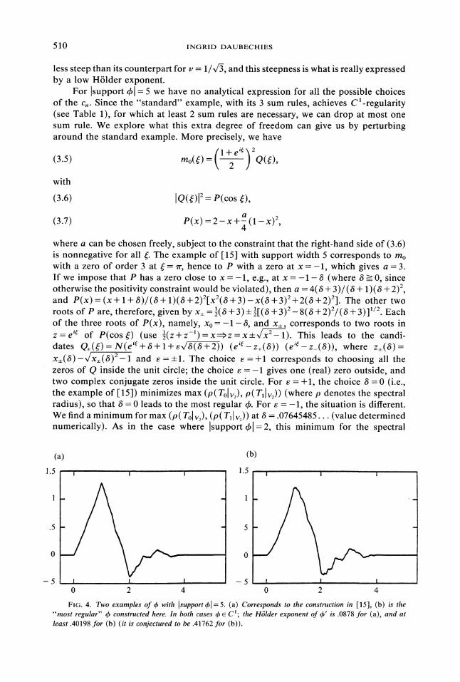
FIG. 4. Two examples of ch with Isupportchl=5. (a) Corresponds to the construction in [15], (b) is the"most regular" qb constructed here. In both cases ch C 1" the H61der exponent of qb’ is .0878 for (a), and at

least .40198 for (b) (it is conjectured to be .41762 for (b)).


radii p(T[v2) corresponds to a degenerate largest eigenvalue of Tllv2, and we findagain that T[v is not diagonalizable. Consequently, we can only hope to establish

h <_- 2(1 + e) max (p( Tol v), p( T[ v2)) (1 + e).74865....

In order to obtain e <.01, we already have to consider a large number of buildingblocks Ta,’’" Ta,,, the longest of which has dj 1 for j 1,..., m, and m->_ 700! Itseems likely that arbitrarily small e can be attained by more work. Figure 4 showsboth the standard example of [15] and the most regular b obtained here for[support b -5. It is apparent that the present example is much more regular; bothfunctions are C (even though the function of [15] seems to have peaks, these peaksare not really sharp--see [llb]), but the H61der exponent of b’ is significantly betterin the example constructed here.

4. Vanishing moments for tb. In this subsection we want to construct b, q withcompact support,

and such that

Isupp 4,[ Isupp 4’1 2M- 1

dx c(x)= 1,

(4.1) f dx xtch(x) 0 for 1,..., L- 1,

dxxlp(x) =0 for l--0,..., L-1.

The need for orthonormal bases with this property first came up in the application ofwavelet bases to numerical analysis in the work of Beylkin, Coifman, and Rokhlin[19]. The desirability of vanishing moments for b is explained in the introduction" if(4.1) is satisfied, then the inner product of 4jk with a smooth function f only dependson f(2Jk) and derivatives off of order =>L. (In a later version of their work, Beylkin,Coifman, and Rokhlin did not require (4.1), however.) Imposing such vanishingmoments on b also increases its symmetry. Because these orthonormal wavelet baseswith vanishing moments for both b and p were requested by Coifman, I have namedthese wavelets coiflets. Condition (4.1) corresponds to a coiflet of order L.

The Fourier transforms of b, q are given by (sc)=I-I= mo(2-sc) q(sc)m(/2)(/2), with

N

mo() Cn ein, ml()= (-1)nc-n+l ein=-eimo(+).=N

Note that the lower limit N in the sum over n will in general not be zero in thissubsection: we have lost our freedom to translate by integers because (4.1) is notinvariant under such translations (the conditions on are translation-invariant, butthe conditions on are not). The conditions (4.1) are equivalent to

(0)=1, (0)=0 forl=l,...,L-1,

(d)(0)=0 for/=O,...,L-1.


In terms of mo, these become

(4.2) mol)(+.a-) =0 for/=0,..., L- 1,

(4.3) too(0) 1, mol)(o)= 0 for l= 1,..., L- 1.

By (4.2), mo has a zero of order L in : r. Consequently, mo has to be of the form

(4.4) too(,) (1 + ei)L

2Q(ei)’

where

(4.5) IQ(e’e)l: + R(cos )j=o j 2 2

and R is an odd polynomial [15]. On the other hand (4.3) implies

(4.6) mo() 1 +(1-ei)LS(e’).

Together, (4.4) and (4.6) lead to L independent linear constraints on the coefficientsof S. Imposing that Q be of the form (4.5), with R an odd polynomial, leads to furtherquadratic constraints. For small values of L, the whole collection of constraint equationscan be solved more or less by hand; for values of L larger than 6, the situation becomesuntractable. We propose, therefore, an approach which from the start satisfies (4.2)and (4.3) (the linear constraints on S are built in), and we tackle (4.5) afterwards.

For the sake of convenience, we restrict ourselves to L even, L 2K. A similaranalysis can be carried out for L odd. We impose that mo be of the form

r (K-l+ k K

Since cos /2= e-e(1 +ee), this clearly has a zero of order 2K at = . On theother hand, (4.7) can be rewritten as (use (1.13))

mo() 1 + sink

csk=0

+ cOS2

This clearly satisfies (4.3). It remains, therefore, to tailor f so that m0 satisfies (1.10).For the sake of convenience we shall use f such that

K’

(4.8) f()= f.e ’’,n=0

i.e., f, 0 for all n < 0. This is by no means the only choice possible; we could alsodecide to distribute the f, as symmetrically around zero as possible, so that the suppoof would be more symmetrical around x =0. It turns out, however, that thissymmetrical choice can lead to larger suppo widths for than (4.8) (this happens,e.g., for K 3). From (4.5) we obtain

(K-l+k)(ksin) ( )rk=+ sin2 f()

(4.9)


where R is an odd polynomial. Rewriting (4.9) leads to

(4.10)

2-l (2K l +J )s2 + sKR(cos ,),+ slf(,)[j=o J

where s2 denotes sin2 (:/2). We shall determine the f, by identifying coefficients of s.Both f()+f() and If(#)l= can be written as polynomials in cos :, hence in s2.

It follows that only the first term in the left-hand side of (4.10), which is independentoff, contains terms in s withj -< K 1. Founately, these terms cancel the correspond-ing terms in s in the right-hand side of (4.10) because of the identity

(4.11) Zk=O k K- k K

(See [26, (5.27) ].)We next concern ourselves with the terms in s, j K,..., 2K- 1. Only the first

two terms in the left-hand side of (4.10) contribute, leading to linear constraints in thef. Define g by

K’

(4.12) f()+f(= 2 g,s.n=0

Using s2 =- e-e(1- ee)2, we find that the f, and g, are related through

4-g,

(4.13)

f=(-1) 4-g fork0.

In practice we will determine the g and then calculate the f and f via (4.13).Identification of the terms in s, j K,..., 2K 1 on both sides of (4.10) gives

=_+ k j-k

’,- j-l-kg=+kj-K-k] j

Using (4.11) again, and substituting j K + l, =0,..., K- 1, we can reduce this to

(4.14) 2 g_ =2=,(o,-, m =o k k K + l- k

This is a system of K linear equations in rain (K, K’ + 1) unknowns. It has no solutionsif K’ + 1 < K. If K’ K 1, then the inveibility of the triangular matrix

Mq= (K-l+i-J)i_j K-lijO

immediately leads to

2K-l+k)gt=2K + k

k=0,...,K-1.


(4.15)

It remains to determine the gK,..., gK,. They are given by the constraint that

k=0 ,=0 kgl+’s+’+]f()

should be an odd polynomial in cos . Since (4.15) can be rewritten as a polynomialof degree K’ in cos sc, this results in [(K’+ 1)/21 equations for K’-K + 1 unknowns.It follows that K’>= 2K 1 (no miraculous cancellations occur). In the examples workedout here, K’= 2K- 1. In these examples a solution has to be found for a system ofK quadratic equations in K unknowns; every such solution corresponds to a coifletof order 2K, with support width 3K- 1.

The system of K equations to be solved can be written out a little more explicitly.Writing x,,, m =0,..., K- 1 for the K unknown gK+m, we have

with

(4.16)

(4.17)

2K-1 min(2K-1,2K-l-I)

I=--(2K --1) k=max (0,-1)

f (1 1/26o)(- 1) 2 k/4-k rI

+ 4-m-Kxm,,=o m+K-k]

fk=(_l)k 2m+2K,,,=,_ m + K k]

4-’-U"x" K <_k<=2K-1.

2K --2il (_ 4-

2j O, K 1 mX e 1) X X x,,.

/=--(2K--2) J=l/I J + m=max(O,j-K+l) j- m

The K equations in the unknowns Xo,..., x:-i are, therefore,

(4.18) fkf2r+, + 4- 2j 0,-1) K 1 +j- mx 0,

=o j=2 + 2r m=max(O,j--K+l) j-- m

where r=0,..., K-1, and where (4.16), (4.17) have to be substituted for the f.As a quadratic system (4.18) can have many solutions or no solutions at all. The

following heuristic argument suggests that (4.18) will have solutions for sufficientlylarge K. We can rewrite (4.7) as

(e +em()=2+2-4+K K =o2k+l K+k(4.19)

Let us concentrate on the first two terms in (4.19). For large K, the coecient ofe(+e tends to

2k+ 1 k K+k + (2k+ 1)’

2K-2, min(j,K-1)(K-l+j-m)I; s 2 xj=0 m=max(O,j--K+l) J m

O<=k<=K-1

On the other hand, the first term in (4.15) can be rewritten as


which is exactly the Fourier coefficient of the characteristic function X(:)= 1 for

I:1 -<- 7r/2, 0 for Iscl _-> 7r/2,

1 1 i(2k+1): -i(2k+l):).X(sc)=+ (-1) g (e +e,--o zr(2k+ 1)

This is, in fact, a perfectly legitimate choice for mo" mo=X leads to (sc) 1 forIsc[_-< zr, 0 otherwise, or b(x)=sin 7rx/Trx. The corresponding wavelet basis is C,satisfies (4.1) for arbitrarily large L, but has rather slow decay at . Our ansatz (4.7)or (4.19) for mo can, therefore, be viewed as a truncation to finite length of X, consistentwith the restrictions (4.2), (4.3), and where an additional f has to be introduced to fit(1.9). Since for K -, X itself already satisfies all the conditions (1.9), (4.2), (4.3), itseems reasonable to hope that for large K, a slight perturbation of X might satisfy(1.9), (4.2), (4.3).

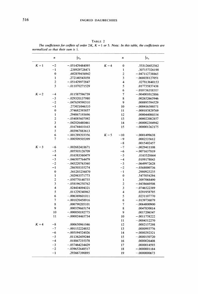
Based on this perturbation argument, we can look for a solution to (4.18) "closeto" Xm=O. For K 1,2,3,4, and 5 we have (1) determined the system (4.18) withthe symbolic manipulation package MACSYMA, (2) found a solution by Newton’smethod, starting from the initial point x,,- 0, m 0,..., K- 1. The resulting mo aretabulated in Table 2. For K 5 the coefficients are given with less precision than forK =< 4 because the roundoff error, even with double precision, was sufficient to perturbdecimals beyond the 10th decimal. Note that Table 2 corrects a mistake in the firstentry in the corresponding Table 8.1 in [25]. Graphs for the corresponding b, q canbe found in [25, Fig. 8.3].

Remarks.(1) The functions 4 and q corresponding to Table 2 are almost symmetric. For

some of these examples, there exists a pair of biorthogonal bases very close to theorthonormal basis (their graphs are almost indistinguishable), which have, moreover,the advantage of corresponding to rational c, (see [21]).

(2) The approach given above has the merit ofgiving a method for the constructionof coiflets of any order L (modulo the solution of a system of L!2 quadratic equationsin L/2 variables). It does not necessarily give the smoothest coiflet of order L, however!For small L, everything can be worked out more or less by hand, and we find somesolutions different from the coiflets given above.

For L 2, the smoothest coiflet is found by substituting

f() a e i + b e2i,rather than (4.8) into (4.7), leading to a less symmetric coiflet with support width 5;in this case support b [-1, 4]. The system of quadratic equations reduces to a singleequation, so that everything can be solved explicitly. We find

a=(s-1)/2, b=(-s+3)/2, withs=+x/T.

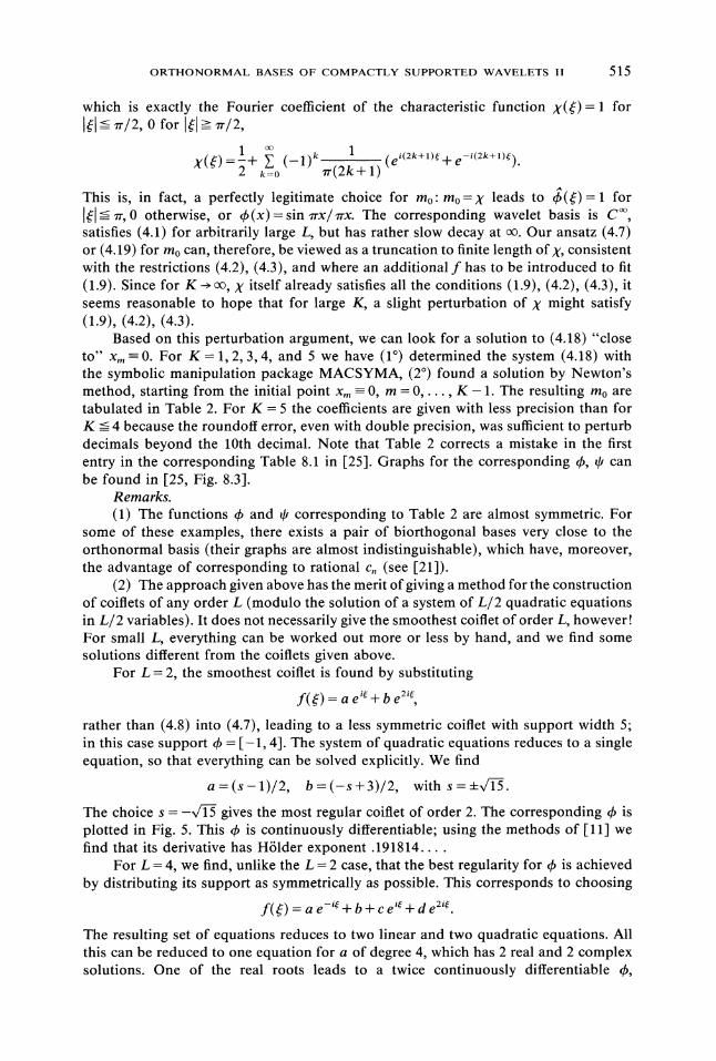
The choice s =-x/] gives the most regular coiflet of order 2. The corresponding b isplotted in Fig. 5. This b is continuously differentiable; using the methods of [11] wefind that its derivative has HSlder exponent .191814

For L 4, we find, unlike the L 2 case, that the best regularity for b is achievedby distributing its support as symmetrically as possible. This corresponds to choosing

f(() a e-i# 4;- b + c e’ + d e2’.

The resulting set of equations reduces to two linear and two quadratic equations. Allthis can be reduced to one equation for a of degree 4, which has 2 real and 2 complexsolutions. One of the real roots leads to a twice continuously differentiable 4,


TABLE 2The coefficients for coiflets of order 2K, K or 5. Note" In this table, the coefficients are

normalized so that their sum is 1.

n 1/2c. n 1/2c.

K= -2 -.051429484095 K= 4-1 .2389297284710 .602859456942

.2721405430582 -.0514299728473 -.011070271529

K=2

K=3

K=4

-4 .011587596739-3 -.029320137980-2 -.047639590310-1 .2730210465350 .574682393857

.2948671936962 -.0540856070923 -.0420264804614 .0167444101635 .0039678836136 -10012892033567 -.000509505399

-6 -.002682418671-5 .005503126709-4 .016583560479-3 -.046507764479-2 -.043220763560-1 .2865033352740 .561285256870

.3029835717732 -.0507701407553 -.0581962507624 .0244340943215 .0112292409626 -.0063696010117 -.0018204589168 .0007902051019 .00032966517410 -.00005019277511 -.000024465734

-8 .000630961046-7 -.001152224852-6 -.005194524026-5 .011362459244-4 .018867235378-3 -.057464234429-2 -.039652648517-1 .293667390895

K=5

0 .553126452562.307157326198

2 -.0471127388653 -.0680381270514 .0278136401535 .0177358374386 -.0107563185177 -.0040010128868 .0026526659469 .00089559452910 -.00041650057111 -.00018382976912 .00004408035413 .00002208285714 -.00000230494215 -.000001262175

-10 -.0001499638-9 .0002535612-8 .0015402457-7 -.0029411108-6 -.0071637819-5 .0165520664-4 .0199178043-3 -.0649972628-2 -.0368000736-1 .29809232350 .5475054294

.30970684902 -.04386605083 -.07465223894 .02919587955 .02311077706 -.01397368797 -.00648009008 .00478300149 .001720654710 -.001175822211 -.000451227012 .000213729813 .000099377614 -.000029232115 -.000015072016 .000002640817 .000001459318 -.000000118419 -.0000000673

ORTHONOIMAL BASES OF COMPACTLY SUPPORTED WAVELETS II 517

|.5

.5

-1 0 2 3 4

FIG. 5. Plot of d for the coiflet of order 2 with the highest regularity.

corresponding to

c_5 -.008089728693,c_4 -.001473073456,c_ .027620978693,

c_2 .000661782050,

C_l -.029586627843,

Co .168333606358,

Cl .503931298301,

c2 .443259223184,

c3 .010862015621,

c4 -.136801026363,

c5 -.004737936078,

c6 .026019488227.

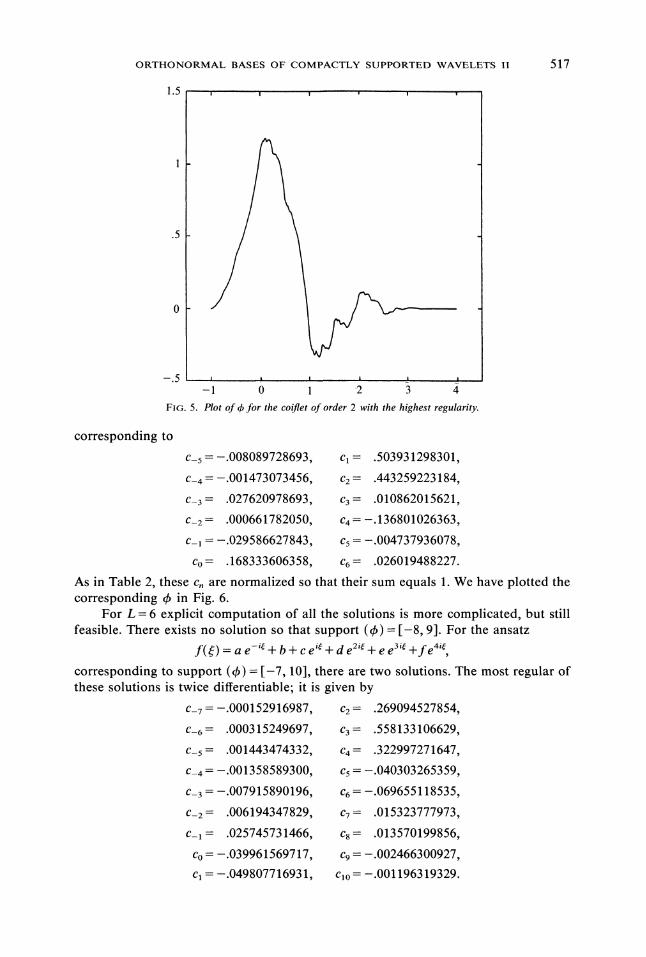
As in Table 2, these c, are normalized so that their sum equals 1. We have plotted thecorresponding b in Fig. 6.

For L 6 explicit computation of all the solutions is more complicated, but stillfeasible. There exists no solution so that support (b)= [-8, 9]. For the ansatz

f() a e-i + b + c e + d e + e e3 +fe4,corresponding to support (b)= [-7, 10], there are two solutions. The most regular ofthese solutions is twice differentiable; it is given by

c_7 -.000152916987,c_6 .000315249697,

c_5= .001443474332,

C_a -.001358589300,

c-3 -.007915890196,

c_ .006194347829,

c-1 .025745731466,

Co -.039961569717,

ca -.049807716931,

c2 .269094527854,

c3 .558133106629,

c4 .322997271647,

c -.040303265359,

c6 -.069655118535,

c7 .015323777973,

c8 .013570199856,

c9 -.002466300927,

Clo -.001196319329.


1.5

--.5-5 0 5FIG. 6. Plot of qb for the most regular coiflet of order 4.

1.5

-.5-5 0 5 10

FIG. 7. Plot of c for the most regular coiflet of order 6, with support b [-7, 11 ].

The function b is plotted in Fig. 7. The coiflets used in 19] for L 2, 4, 6 correspondto the scaling functions b in Figs. 5, 6, and 7.

Acknowledgments. I would like to thank everyone who suggested the usefulnessof the variations constructed in this paper, in particular, M. Basseville, G. Beylkin, A.Cohen, R. Coifman, and Y. Meyer.


REFERENCES

[1] J. MORLET, Sampling theory and wave propagation, in Issues on Acoustic Signal/Image Processingand Recognition, C. H. Chen, ed., NATO ASI, Springer-Verlag, New York, 1983.

[2] A. GROSSMANN AND J. MORLET, Decomposition of Hardy functions into square integrable waveletsof constant shape, SIAM J. Math. Anal., 15 (1984), pp. 723-736.

[2a] P. GOUr’ILLAUD, A. GrOSSMANN, AND J. MORLET, Cycle-octave and related transforms in seismic

signal analysis, Geoexploration, 23 (1984), p. 85.[3] A. GROSSMANN, J. MORLET, AND T. PAUL, Transforms associated to square integrable group

representations, I, J. Math. Phys., 26 (1985), pp. 2473-2479; II, Ann. Inst. H. Poincar, 45 (1986),pp. 293-309.

[4] I. DAUBECHIES, A. GROSSMANN, AND Y. MEYER, Painless non-orthogonal expansions, J. Math.Phys., 27 (1986), pp. 1271-1283.

[4a], The wavelet transform, time-frequency localization and signal analysis, IEEE Trans. Inform.Theory, 34 (1988), pp 605-612.

[5] P. AUSCHZR, Ondelettesfractales et applications, Ph.D. thesis, CEREMADE, University of Paris IX,1989.

[6] S. MALLAT, Multiresolution approximation and wavelets, Trans. Amer. Math. Soc., 315 (1989), pp. 69-88.[7] Y. MEYER, Ondelettes, function splines, et analyses gradues, Lectures given at the Mathematics

Department, University of Torino, 1986.[8] G. BATTLE, A block spin construction of ondelettes. Part I: Lemair functions, Comm. Math. Phys.,

110 (1987), pp. 601-615.[9] P. G. LEMARII, Une nouvelle base d’ondelettes de L2(n), J. Math. Pures Appl., to appear.

[10] Y. MEYER, Ondelettes, opdrateurs et analyse non lindaire, Hermann, Paris, 1990.[lla] I. DAUBECHIES AND J. LAGARIAS, Two-scale difference equations, I. Global regularity of solutions,

SIAM J. Math. Anal., 22 (1991), pp. 1388-1410.[llb], Two-scale difference equations, II. Local regularity, infinite products of matrices and fractals,

SIAM J. Math. Anal., 23 (1992), pp. 1031-1079.[12] W. LAWTON, Tight frames of compactly supported wavelets, J. Math. Phys., 31 (1990), pp. 1898-1901.[13] A. COHEN, Ondelettes, analyses multirdsolution et filtres mirroir en quadrature, Ann. Inst. Poincar6,

Analyse non lin6aire, 7 (1990), pp. 439-459.[14] G. DESLAURIERS AND S. DUBUC, Interpolation dyadique, in Fractals, dimensions non entires et

applications, G. Cherbit, ed., Masson, Paris, 1987, pp. 44-56.[15] I. DAUBECHES, Orthonormal basis of compactly supported wavelets, Comm. Pure Appl. Math., 41

(1988), pp. 909-996.16] WaveletsNtime-frequency methods and phase space, Proceedings of the December ’87 Conference,

Marseille, France, J. M. Combes, A. Grossmann, and Ph. Tchamitchian, eds., Springer, Berlin,1989.

[17] G. POLYA AND G. SZEG6, Aufgaben und Lehrsiitze aus der Analysis, Vol. II, Springer, Berlin, 1971.[18] G. BATTLE AND P. FEDERBUSH, Ondelettes and phase cell cluster expansions: a vindication, Comm.

Math. Phys., 109 (1987), pp. 417-419.[19] G. BEYLKIN, R. COIFMAN, AND V. ROKHLIN, Fast wavelet transforms and numerical algorithms. I,

Comm. Pure Appl. Math., 44 (1991), pp. 141-183.[20] Y. MEYER, Wavelets with compact support, Zygmund lectures, University of Chicago, Chicago, IL,

1987.121] A. COHEN, I. DAUBECHES, AND J. C. FEAUVEAU, Biorthogonal bases ofcompactly supported wavelets,

Comm. Pure Appl. Math., 45 (1992), pp. 485-560.[22] G. BATTLE, Phase space localization theorem for ondelettes, J. Math. Phys., 30 (1989), pp. 2195-2196.[23] A. COHEN AND J. P. CONZE, Rdgularitd des bases d’ondelettes et mesures ergodiques, Rev. Mat.

Iberoamericana, to appear.[24] H. VOLKMER, On the regularity of wavelets, IEEE Trans. Inform. Theory, 38 (1992), pp. 872-876.[25] I. DAUBECHIES, Ten lectures on wavelets, CBMS-NSF Regional Conf. Ser. in Appl. Math., Society

for Industrial and Applied Mathematics, Philadelphia, PA, 1992.[26] R. L. GRAHAM, D. E. KNUTH, AND O. PATASHNIK, Concrete Mathematics, Addison-Wesley,

Reading, MA, 1989.

q%(x) 2-;/2q(2-;x- L2(E).

Documents

Transcript of q%(x) 2-;/2q(2-;x- L2(E).