1

Query Processing + Optimization: Outline• Operator Evaluation Strategies

Query processing in generalSelectionJoin

• Query OptimizationHeuristic query optimizationCost-based query optimization

• Query Tuning

2

Query Processing + Optimization• Operator Evaluation Strategies

SelectionJoin

• Query Optimization• Query Tuning

3

Architectural Context

DBMS

DDL Statements

Privileged Commands

InteractiveQuery

Precompiler

ApplicationPrograms

Application Programmers

Host LanguageCompiler

CannedTransactions

DDLStatements

QueryCompiler

Query ExecutionPlan

Run-timeEvaluator

Transaction andData Manager

Data Dictionary Data Files

DDLCompiler

DBA Staff Casual Users ParametricUsers

4

Evaluation of SQL Statement• The query is evaluated in a different order.

The tables in the from clause are combined using Cartesian products.The where predicate is then applied.The resulting tuples are grouped according to the group by clause.The having predicate is applied to each group, possibly eliminating some groups.The aggregates are applied to each remaining group.The select clause is performed last.

5

Overview of Query Processing

Scanning, Parsing, andSemantic Analysis

Query Optimization

Query Code Generator

Runtime DatabaseProcessor

Intermediate form of query

Execution Plan

Code to execute the query

Result of query

Query in high-level language1. Parsing and translation2. Optimization3. Evaluation4. Execution

6

Selection Queries• Primary key, point

σFilmID = 2 (Film)• Point

σTitle = ‘Terminator’ (Film)• Range

σ1 < RentalPrice < 4 (Film)• Conjunction

σType = ‘M’ ∧ Distributor = ‘MGM’ (Film)• Disjunction

σPubDate < 2004 ∨ Distributor = ‘MGM’ (Film)

7

Selection Strategies• Linear search

Expensive, but always applicable.• Binary search

Applicable only when the file is appropriately ordered.• Hash index search

Single record retrieval; does not work for range queries.Retrieval of multiple records.

• Clustering index searchMultiple records for each index item.Implemented with single pointer to block with first associated record.

• Secondary index searchImplemented with dense pointers, each to a single record.

8

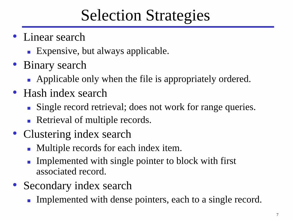
Selection Strategies for Conjunctive Queries• Use any available indices for attributes involved in

simple conditions.If several are available, use the most selective index. Then check each record with respect to the remaining conditions.

• Attempt to use composite indices. This can be very efficient.

• Do intersection of record pointers.If several indices with record pointers are applicable to the selection predicate, retrieve and intersect the pointers. Then retrieve (and check) the qualifying records.

• Disjunctive queries provide little opportunity for smart processing.

9

Joins• Join Strategies

Nested loop joinIndex-based joinSort-merge joinHash join

• Strategies work on a per block (not per record) basis.Need to estimate #I/Os (block retrievals)

• Relation sizes and join selectivities impact join cost.Query selectivity = #tuples in result / #candidates

‘More selective’ means smaller ‘selectivity value’For join, #candidates is the size of Cartesian product

10

Nested Loop Join and Index-Based Join• Nested loop join

Exhaustive comparison (i.e., brute force approach)The ordering (outer/inner) of files and allocation of buffer space is important.

• Index-based joinRequires (at least) one index on a join attribute.At times, a temporary index is created for the purpose of a join.The ordering (outer/inner) of files is important.

11

r

Nested Loop• Basically, for each block of the outer table (r), scan the

entire inner table (s). Requires quadratic time, O(n2)Improved when buffer is used.

s

Main MemoryBuffer

OutputScan

s

spill when full

r

Outer

Inner

12

Example of Nested-Loop JoinCustomer nC.CustomerID = CO.EmpId CheckedOut

• ParametersrCheckedOut = 40.000 rCustomer = 200bCheckedOut = 2.000 bCustomer = 10nB = 6 (size of main memory buffer)

• Algorithm:repeat: read (nB - 2) blocks from outer relation

repeat: read 1 block from inner relationcompare tuples

• Cost: bouter + ( ⎡bouter/ (nB -2)⎤ ) × binner

• CheckedOut as outer: 2.000 + ⎡2.000/4⎤ × 10 = 7.000• Customer as outer: 10 + ⎡10/4⎤ × 2.000 = 6.010

13

ss

Index-based Join• Requires (at least) one index on a join attribute

A temporary index can be created

r

Output

Scan

spill when full

r

index on r

if joins

Main Memory

for each record ofs, query in indexOuter

14

Example of Index-Based JoinCustomer nC.CustomerID = CO.EmpId CheckedOut

• Cost: bouter + router × cost use of index• Assume that the video store has 10 employees.

There are 10 distinct EmpIDs in CheckedOut.• Assume 1-level index on CustomerID of Customer.• Iterate through all 40.000 tuples in CheckedOut (outer

rel.)2.000 disk reads (bCheckedOut) to scan CheckedOutFor each CheckedOut tuple, search for matching Customertuples using index.

0 disk reads for index (in main memory) + 1 disk read for actual data block

• Cost: 2.000 + 40.000 × (0 + 1) = 42.000

15

Sort-Merge Join

unsortedr

sortedr

r1

r2

rn

sortedr

• Sort each relation using multiway merge-sort• Perform merge-join

sorteds

Main Memory

••••••••••••

Output

Match•••

Scan

Scan

16

External or Disk-based Sorting• Relation on disk often too large to fit into memory• Sort in pieces, called runs

r

Main MemoryBuffer (N blocks)

Scan Output when sorted

r

Unsorted relation(M blocks)

r1

r2

rM div N

•••

rlast

Runs(M div N runs each of

size N blocks, and maybe one last run of < N leftover blocks)

17

Output when merged

External or Disk-based Sorting, Cont.• Runs are now repeatedly merged• One memory buffer used to collect output

Main MemoryBuffer (N blocks)

output

sorted runs(N blocks each)

m1

m2

mlast - 1

•••

mlast

Merged runs((M div N) div N-1) runs each of

size N*N-1 blocks, and maybe one last run of < N*N-1 leftover blocks)

r1

r2

rM div N

•••

rlast

rN - 1

•••

Main MemoryBuffer (N blocks)

output

18

External Sorting (Multiway Merge Sort)

32 5 1712 1 14 8 3 3130232629 2 2511 6 7 151628 4 9 221821102013272419

5 121732 1 3 8 14 23263031 2 112529 6 7 1516 4 9 2228 10182021 13192427

1 3 5 8 1214172326303132 2 4 6 7 9 11151622252829 1013181920202427

1 2 3 4 5 6 7 8 9 1011121314151617181920212223242526272829303132

Orginal rel.

Initial runs

First merge

Second merge

• Buffer size is nB = 4 (N)

• Cost: 2 × brelation + 2 × brelation × ⎡lognB - 1 (brelation/nB)⎤• 2 × 32 + 2 × 32 × log3(32/4) = 192

19

Example of Sort-Merge Join• Cost to sort CheckedOut (bCheckedOut= 10)

CostSort ChecedOut = 2 × 2.000 + 2 × 2.000 × ⎡log5(2.000/6)⎤ = 20.000• Cost to sort Customer relation (bCustomer= 10)

CostSort Customer= 2 × 10 + 2 × 10 × ⎡log5(10/6)⎤ = 40• Cost for merge join

Cost to scan sorted Customer + cost to scan sorted CheckedOutCostmerge join= 10 + 2.000 = 2.010

• Costsort-merge join = CostSort Customer + CostSort ChecedOut + Costmerge join

• Costsort-merge join= 20.000 + 40 + 2.010 = 22.050

20

Hash Join• Hash each relation on the join attributes• Join corresponding buckets from each relation

Relationr

r1

r2

rn

•••

r1

r2

rn

•••

s1

s2

sn

•••

n

n

n

r2 n s2

r1 n s1

rn n sn

Buckets from r Buckets from s

Hash r (same for s) Join corresponding r and s buckets

21

Partitioning Phase• Partitioning phase: r divided into nh partitions. The

number of buffer blocks is nB. One block used for reading r. (nh = nB -1)

Similar with relation sI/O cost: 2 × (br + bs)

nB main memory buffers DiskDisk

Relationr or s

OUTPUT

2INPUT

1

hashfunction

hnB -1

Partitions

1

2

nB -1

. . .

22

Joining Phase• Joining (or probing) phase: nh iterations where rin si.

Load ri into memory and build an in-memory hash index on it using the join attribute. (h2 needed, ri called build input)Load si, for each tuple in it, join it with ri using h2. (si called probe input)I/O cost: br + bs + 4 × nh (each partition may have a partially filled block)

One write and one read for each partially filled block

Partitionsof r & s

Input bufferfor si

In-memory hash table for partition ri (< nB -1 blocks)

nB main memory buffersDisk

Output buffer

Disk

Join ResultHashfunc.h2

h2

23

Hash Join Cost• CostTotal = Cost Partitioning + CostJoining

= 3 × (br + bs) + 2 × nh

• Cost = 3 × (2000 + 10) + 2 × 5 = 6040

• Any problem not considered?What if nh > nB -1? I.e., more partitions than available buffer blocks!How to solve it?

nB main memory buffersDisk

Relationr or s

OUTPUT

2INPUT

1

hashfunction

hnB -1

. . . nB

24

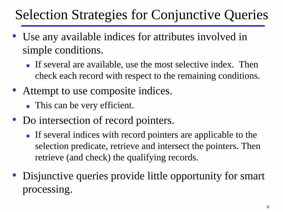
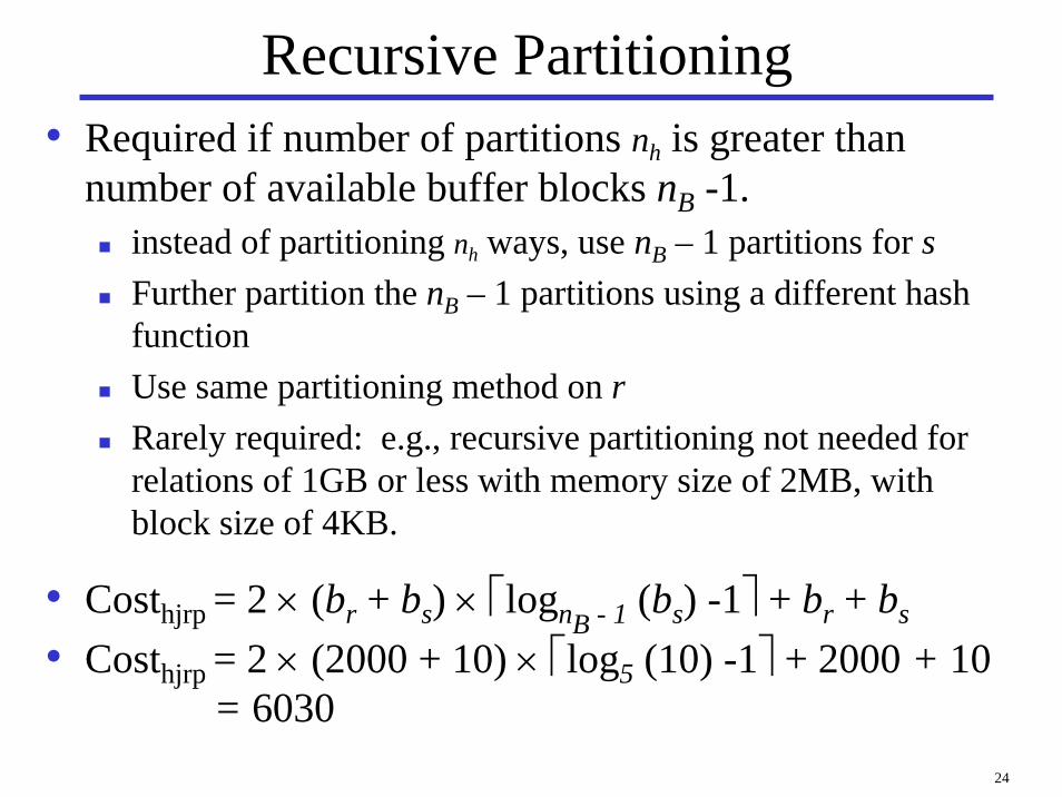
Recursive Partitioning• Required if number of partitions nh is greater than

number of available buffer blocks nB -1.instead of partitioning nh ways, use nB – 1 partitions for sFurther partition the nB – 1 partitions using a different hash functionUse same partitioning method on rRarely required: e.g., recursive partitioning not needed for relations of 1GB or less with memory size of 2MB, with block size of 4KB.

• Costhjrp = 2 × (br + bs) × ⎡lognB - 1 (bs) -1⎤ + br + bs

• Costhjrp = 2 × (2000 + 10) × ⎡log5 (10) -1⎤ + 2000 + 10= 6030

25

Cost and Applicability of Join Strategies• Nested-loop join

Brute-forceCan handle all types of joins (=, <, >)

• Index-based joinRequires minimum one index on join attributes

• Sort-merge joinRequires that the files are sorted on the join attributes.Sorting can be done for the purpose of the join.A variation is also applicable when secondary indices are available instead.

• Hash joinRequires good hashing functions to be available.Performance best if smallest relation fits in memory. ?

26

Query Processing + Optimization• Operator Evaluation Strategies• Query Optimization

Heuristic Query OptimizationCost-based Query Optimization

• Query Tuning

27

Query Optimization• Aim: Transform query into faster, equivalent query

query

• Heuristic (logical) optimizationQuery tree (relational algebra) optimizationQuery graph optimization

• Cost-based (physical) optimization

equivalent query 1

equivalent query 2

equivalent query n

...fasterquery

28

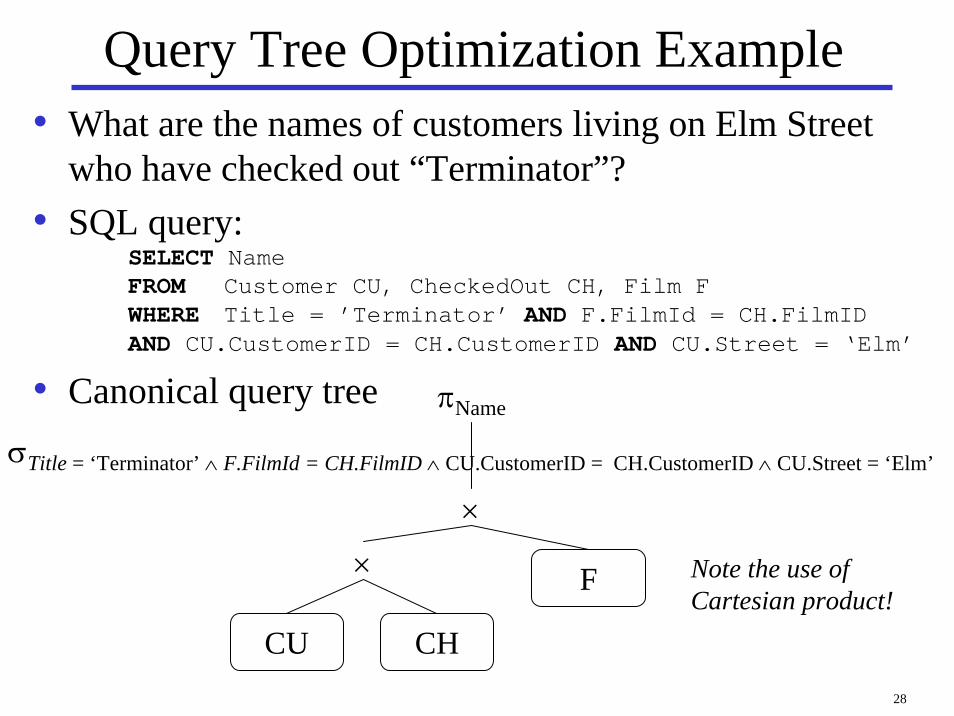
Query Tree Optimization Example• What are the names of customers living on Elm Street

who have checked out “Terminator”?• SQL query:

SELECT NameFROM Customer CU, CheckedOut CH, Film FWHERE Title = ’Terminator’ AND F.FilmId = CH.FilmIDAND CU.CustomerID = CH.CustomerID AND CU.Street = ‘Elm’

• Canonical query tree

CU CH

F×

×

πName

σTitle = ‘Terminator’ ∧ F.FilmId = CH.FilmID ∧ CU.CustomerID = CH.CustomerID ∧ CU.Street = ‘Elm’

Note the use of Cartesian product!

29

Apply Selections Early

CU

CH

F×

×

πName

σStreet = ‘Elm’

σCU.CustomerID = CH.CustomerID σTitle = ‘Terminator’

σ F.FilmId = CH.FilmID

30

Apply More Restrictive Selections Early

F

CH

CU×

×

πName

σTitle = ‘Terminator’

σ F.FilmId = CH.FilmID σStreet = ‘Elm’

σ CU.CustomerID = CH.CustomerID

31

Form Joins

F

CH CU

n F.FilmId = CH.FilmID

n CU.CustomerID = CH.CustomerID

σTitle = ‘Terminator’

σStreet = ‘Elm’

πName

32

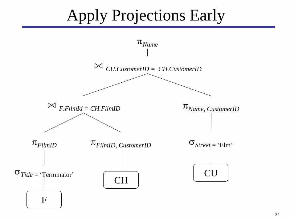
Apply Projections Early

F

CHCU

πName

σTitle = ‘Terminator’

n F.FilmId = CH.FilmID

σStreet = ‘Elm’

n CU.CustomerID = CH.CustomerID

πFilmID πFilmID, CustomerID

πName, CustomerID

33

Some Transformation Rules• Cascade of σ: σc1 ∧ c2 ∧ ... ∧ cn

(R) = σc1(σc2

(...(σcn(R))...))

• Commutativity of σ: σc1(σc2

(R)) = σc2(σc1

(R))• Commuting σ with π: πL(σc (R)) = σc(πL(R))

Only if c involves solely attributes in L.

• Commuting σ with n : σc (R n S) = σc (R) n SOnly if c involves solely attributes in R.

• Commuting σ with set operations: σc(R θ S) = σc(R) θ σc(S)Where θ is one of ∪, ∩, or -.

• Commutativity of ∪, ∩, and n: R θ S = S θ RWhere θ is one of ∪, ∩ and n.

• Associativity of n, ∪, ∩: (R θ S) θ T = R θ (S θ T)

34

Transformation Algorithm Outline• Transform a query represented in relational algebra to

an equivalent one (generates the same result.)

• Step 1: Decompose σ operations.• Step 2: Move σ as far down the query tree as possible.• Step 3: Rearrange leaf nodes to apply the most

restrictive σ operations first.• Step 4: Form joins from × and subsequent σ operations.• Step 5: Decompose π and move down the query tree as

far as possible.• Step 6: Identify candidates for combined operations.

35

Heuristic Query Optimization Summary• Heuristic optimization transforms the query-tree by

using a set of rules (Heuristics) that typically (but not in all cases) improve execution performance.

Perform selection early (reduces the number of tuples)Perform projection early (reduces the number of attributes)Perform most restrictive selection and join operations (i.e. with smallest result size) before other similar operations.

• Generate initial query tree from SQL statement.• Transform query tree into more efficient query tree, via

a series of tree modifications, each of which hopefully reduces the execution time.

• A single query tree is involved.

36

Cost-Based Optimization• Use transformations to generate multiple candidate

query trees from the canonical query tree.• Statistics on the inputs to each operator are needed.

Statistics on leaf relations are stored in the system catalog.Statistics on intermediate relations must be estimated; most important is the relations' cardinalities.

• Cost formulas estimate the cost of executing each operation in each candidate query tree.

Parameterized by statistics of the input relations.Also dependent on the specific algorithm used by the operator.Cost can be CPU time, I/O time, communication time, main memory usage, or a combination.

• The candidate query tree with the least total cost is selected for execution.

37

Relevant Statistics• Per relation

Tuple sizeNumber of tuples (records): rLoad factor (fill factor), percentage of space used in each blockBlocking factor (number of records per block): bfrRelation size in blocks: bRelation organizationNumber of overflow blocks

38

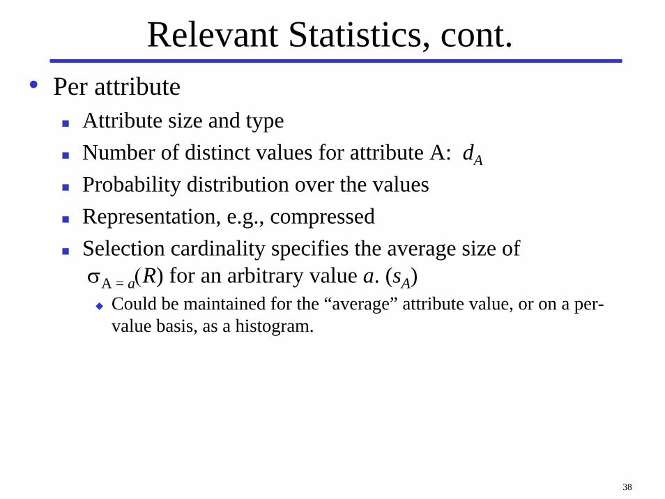
Relevant Statistics, cont.• Per attribute

Attribute size and typeNumber of distinct values for attribute A: dA

Probability distribution over the valuesRepresentation, e.g., compressedSelection cardinality specifies the average size of σA = a(R) for an arbitrary value a. (sA)

Could be maintained for the “average” attribute value, or on a per-value basis, as a histogram.

39

Relevant Statistics, cont.• Per Index

Base relationIndexed attribute(s)Organization, e.g., B+-Tree, Hash, ISAMClustering index?On key attribute(s)?Sparse or dense?Number of levels (if appropriate)Number of first-level index blocks: b1

• GeneralAvailable main memory blocks: N

40

Cost Estimation Example

F

RCU

πName

σTitle = ‘Terminator’

⋈F.FilmId = R.FilmID

σStreet = ‘Elm’

⋈CU.CustomerID = R.CustomerID

πFilmID πFilmID, CustomerID

πFilmID, CustomerID, Name

1

2 3

4

41

Operation 1: σ followed by a π• Statistics

Relation statistics: rFilm= 5,000 bFilm= 50Attribute statistics: sTitle= 1Index statistics: Secondary Hash Index on Title.

• Result relation size: 1 tuple.

• Operation: Use index with ‘Terminator’, then project on FilmID. Leave result in main memory (1 block).

• Cost (in disk accesses): C1 = 1 +1 = 2

42

Operation 2: n followed by a π• Statistics

Relation statistics: rCheckedOut= 40,000 bCheckedOut= 2,000Attribute statistics: sFilmID= 8Index statistics: Secondary B+-Tree Index for CheckedOut on FilmID with 2 levels.

• Result relation size: 8 tuples.

• Operation: Index join using B+-Tree, then project on CustomerID. Leave result in main memory (one block).

• Cost: C2 = 1 +1 + 8 = 10

43

Operation 3: σ followed by a π• Statistics

Relation statistics: rCustomer= 200 bCustomer= 10Attribute statistics:sStreet= 10

• Result relation size: 10 tuples.

• Operation: Linear search of Customer. Leave result in main memory (one block).

• Cost: C3 = 10

44

Operation 4: n followed by a π• Operation: Main memory join on relations in main

memory.

• Cost: C4 = 0

• Total cost: 220101024

1=+++== ∑

=iiCC

45

Comparison• Heuristic query optimization

Sequence of single query plansEach plan is (presumably) more efficient than the previous.Search is linear.

• Cost-based query optimizationMany query plans generated.The cost of each is estimated, with the most efficient chosen.Search is multi-dimensional, usually using dynamic programming. Still can be very expensive.

• Hybrid waySystems may use heuristics to reduce the number of choices that must be made in a cost-based fashion.

46

Query Processing + Optimization• Operator Evaluation Strategies• Query Optimization• Query Tuning

47

Query Tuning• Query optimization is a very complex task.

Combinatorial explosion.The task is to find one good query evaluation plan, not the best one.

• No optimizer optimizes all queries adequately.• There is a need for query tuning.

All optimizers differ in their ability to optimize queries, making it difficult to prescribe principles.

• Having to tune queries is a fact of life.Query tuning has a localized effect and is thus relatively attractive.It is a time-consuming and specialized task.It makes the queries harder to understand.However, it is often a necessity.This is not likely to change any time soon.

48

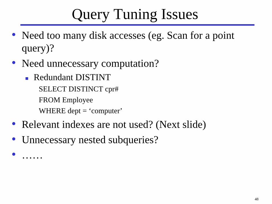
Query Tuning Issues• Need too many disk accesses (eg. Scan for a point

query)?• Need unnecessary computation?

Redundant DISTINTSELECT DISTINCT cpr#FROM EmployeeWHERE dept = ‘computer’

• Relevant indexes are not used? (Next slide)• Unnecessary nested subqueries?• ……

49

Join on Clustering Index, and IntegerSELECT Employee.cpr#FROM Employee, StudentWHERE Employee.name = Student.name-->SELECT Employee.cpr#FROM Employee, StudentWHERE Employee.cpr# = Student.cpr#

50

Nested Queries• Nested block is optimized independently, with the outer tuple

considered as providing a selection condition.• Outer block is optimized with the cost of ‘calling’ nested block

computation taken into account.• Implicit ordering of these blocks means that some good

strategies are not considered. The non-nested version of the query is typically optimized better.

SELECT S.snameFROM Sailors SWHERE EXISTS

(SELECT *FROM Reserves RWHERE R.bid=103 AND R.sid=S.sid)

Nested block to optimize:SELECT *FROM Reserves RWHERE R.bid=103

AND S.sid= outer valueEquivalent non-nested query:SELECT S.snameFROM Sailors S, Reserves RWHERE S.sid=R.sid

AND R.bid=103

51

Unnesting Nested Queries• Uncorrelated sub-queries with aggregates.

Most systems would compute the average only once.SELECT ssnFROM empWHERE salary > (SELECT AVG(salary) FROM emp)

• Uncorrelated sub-queries without aggregates.SELECT ssnFROM empWHERE dept IN (SELECT dept FROM techdept)

Some systems may not use emp's index on dept, so a transformation is desirable.SELECT ssnFROM emp, techdeptWHERE emp.dept = techdept.dept

When is this acceptable?

52

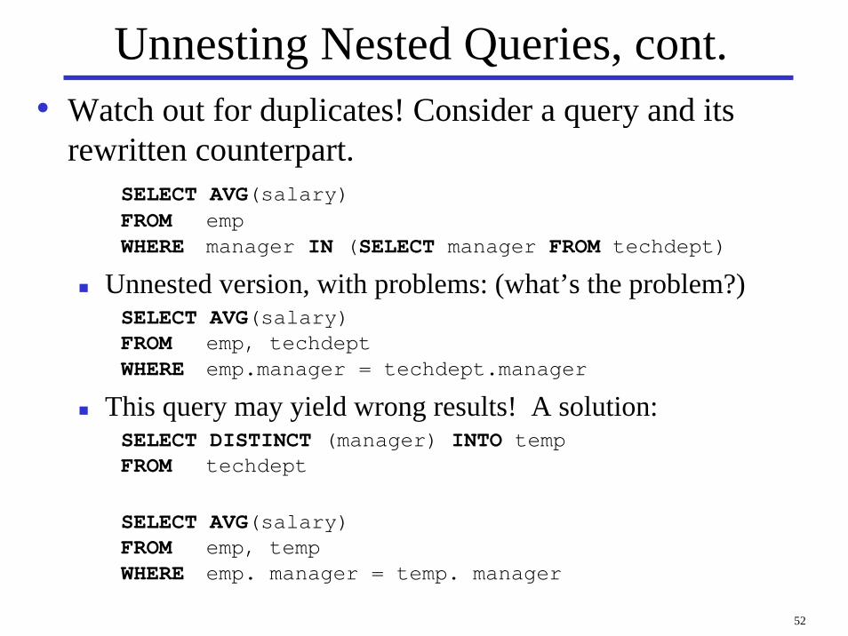
Unnesting Nested Queries, cont.• Watch out for duplicates! Consider a query and its

rewritten counterpart.SELECT AVG(salary)FROM empWHERE manager IN (SELECT manager FROM techdept)

Unnested version, with problems: (what’s the problem?)SELECT AVG(salary)FROM emp, techdeptWHERE emp.manager = techdept.manager

This query may yield wrong results! A solution:SELECT DISTINCT (manager) INTO tempFROM techdept

SELECT AVG(salary)FROM emp, tempWHERE emp. manager = temp. manager

53

Summary• Query processing & optimization is the heart of a

relational DBMS.• Heuristic optimization is more efficient to generate, but

may not yield the optimal query evaluation plan.• Cost-based optimization relies on statistics gathered on

the relations (the default in most DBMSs).• Until query optimization is perfected, query tuning will

be a fact of life.