Query Processing and Optimization. Query Processing Efficient Query Processing crucial for good or...
88
Query Processing and Optimization
-
Upload
elijah-ward -
Category
Documents
-
view
259 -
download
1
Transcript of Query Processing and Optimization. Query Processing Efficient Query Processing crucial for good or...

Query Processing and Optimization
Query Processing
• Efficient Query Processing crucial for good or even effective operations of a database
• Query Processing depends on a variety of factors, not everything under the control of the DBMS
• Insufficient or incorrect information can result in vastly ineffective plans
• Query Cataloging

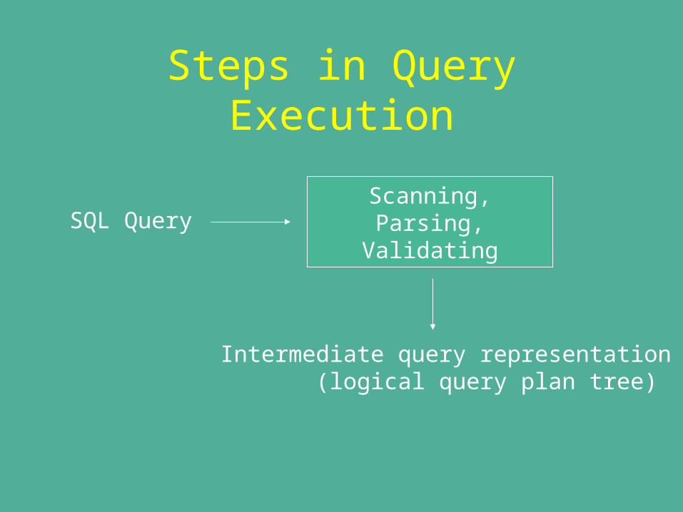
Steps in Query Execution
SQL QueryScanning,Parsing,
Validating
Intermediate query representation (logical query plan tree)
Steps in Query Execution
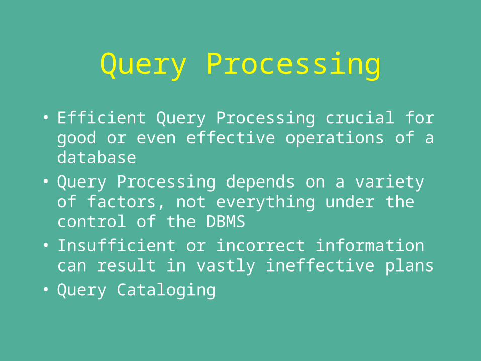
IntermediateQueryRepresentation
QueryOptimizer
Query Execution Plan(physical query plan tree)

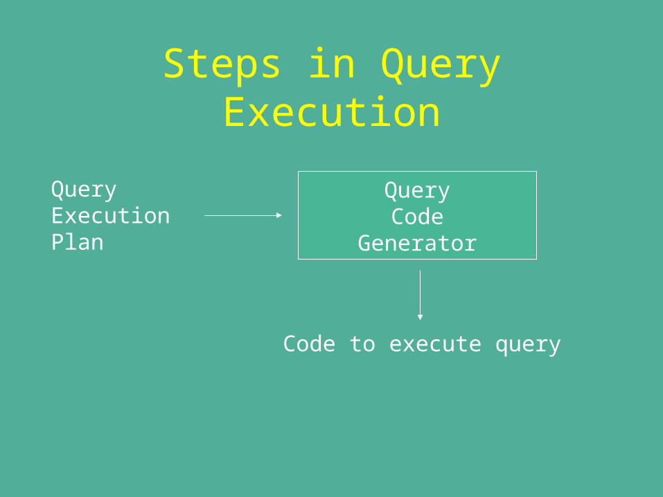
Steps in Query Execution
Query ExecutionPlan
QueryCode
Generator
Code to execute query

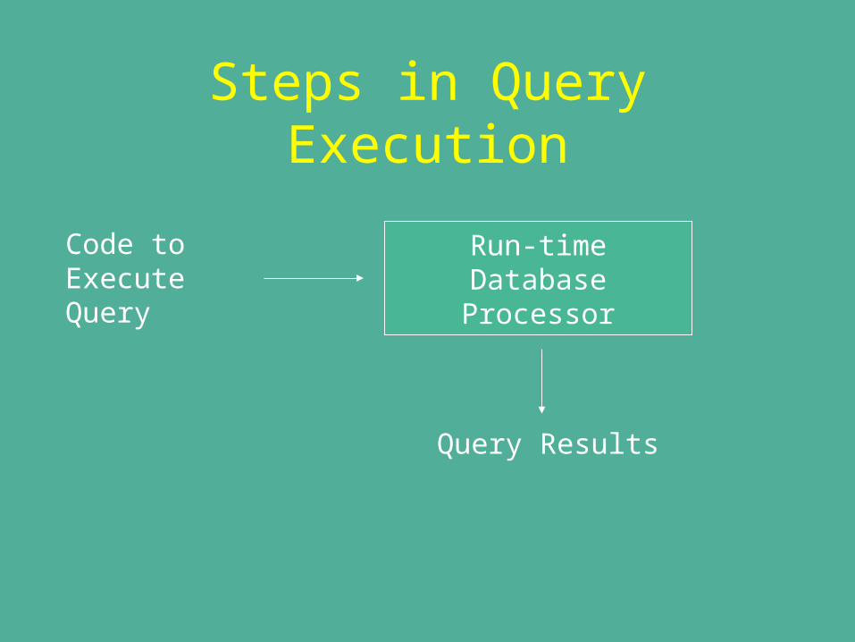
Steps in Query Execution
Code to ExecuteQuery
Run-timeDatabaseProcessor
Query Results
Query Processing
• Intermediate Form– Usually a relational algebra form of the
SQL query – Uses heuristics and cost-based measures
for optimization
• Physical Query Plan– In a language that is interpreted and
executed on the machine or compiled into machine code.
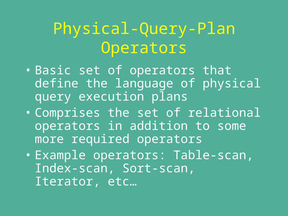
Physical-Query-Plan Operators
• Basic set of operators that define the language of physical query execution plans
• Comprises the set of relational operators in addition to some more required operators
Physical-Query-Plan Operators
• Table scan operator: – Scan and return an entire relation R – Scan and return only those tuples of R that
satisfy a given predicate
• Table scan: reading all blocks of a sorted data file in sequence
• Index scan: Use an index to read al blocks of a data file in sequence
Sorting while Scanning
• Sort-scan operator sorts a relation R while scanning it into memory– If sorting is done on an indexed key
attribute, no need to do anything; scanning will read R in sorted order
– If R is small enough to fit in main memory, perform sorting after scanning
– Else, use external sort-merge techniques to implement sort-scan
Iterators
• Iterators are physical-query-plan operators that comprise of three stages: – Open() where an iteratable object (such as
a relation is opened) – GetNext() returns the next element of the
object – Close() closes control on the object.
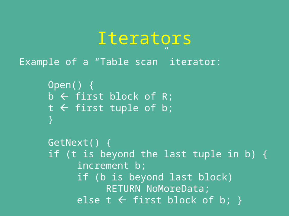
IteratorsExample of a “Table scan” iterator:
Open() { b first block of R; t first tuple of b; }
GetNext() {if (t is beyond the last tuple in b) {
increment b; if (b is beyond last block)
RETURN NoMoreData; else t first block of b; }
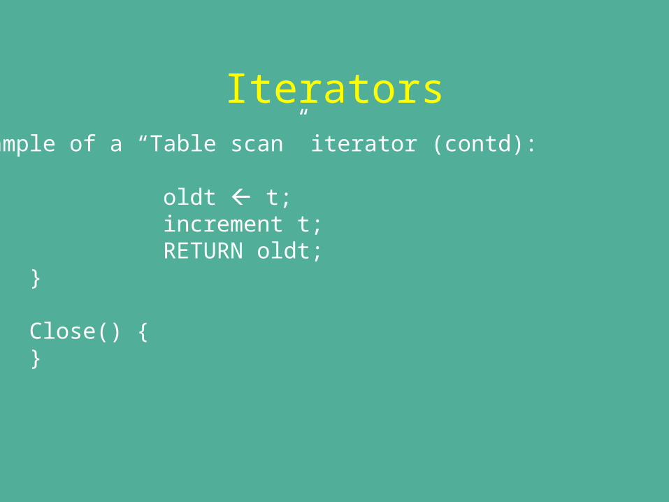
IteratorsExample of a “Table scan” iterator (contd):
oldt t; increment t; RETURN oldt;
}
Close() {}
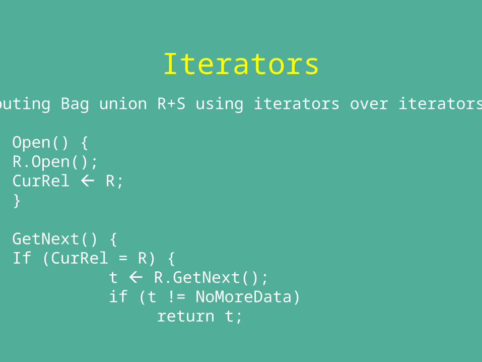
IteratorsComputing Bag union R+S using iterators over iterators:
Open() {R.Open(); CurRel R; }
GetNext() { If (CurRel = R) {
t R.GetNext(); if (t != NoMoreData)
return t;
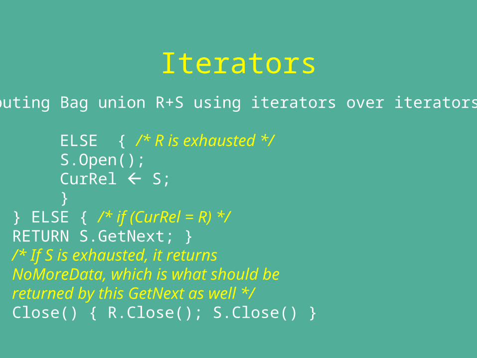
IteratorsComputing Bag union R+S using iterators over iterators:
ELSE { /* R is exhausted */S.Open(); CurRel S; }
} ELSE { /* if (CurRel = R) */ RETURN S.GetNext; }/* If S is exhausted, it returns NoMoreData, which is what should bereturned by this GetNext as well */ Close() { R.Close(); S.Close() }

Database Access Algorithms
Algorithms for database access can be broadly divided in the following categories:
– Sorting-based methods – Hash-based methods– Index-based methods
Physical-Query-Plan Operator Types
• Tuple-at-a-time unary operators: – Can read only one block at a time and required to
work with only one tuple
• Full-relation unary operators: – Requires knowledge of all or most of the relation.
Read into memory for small relations in one-pass algorithms
• Full-relation binary operators:– Same as above, but on two relations.
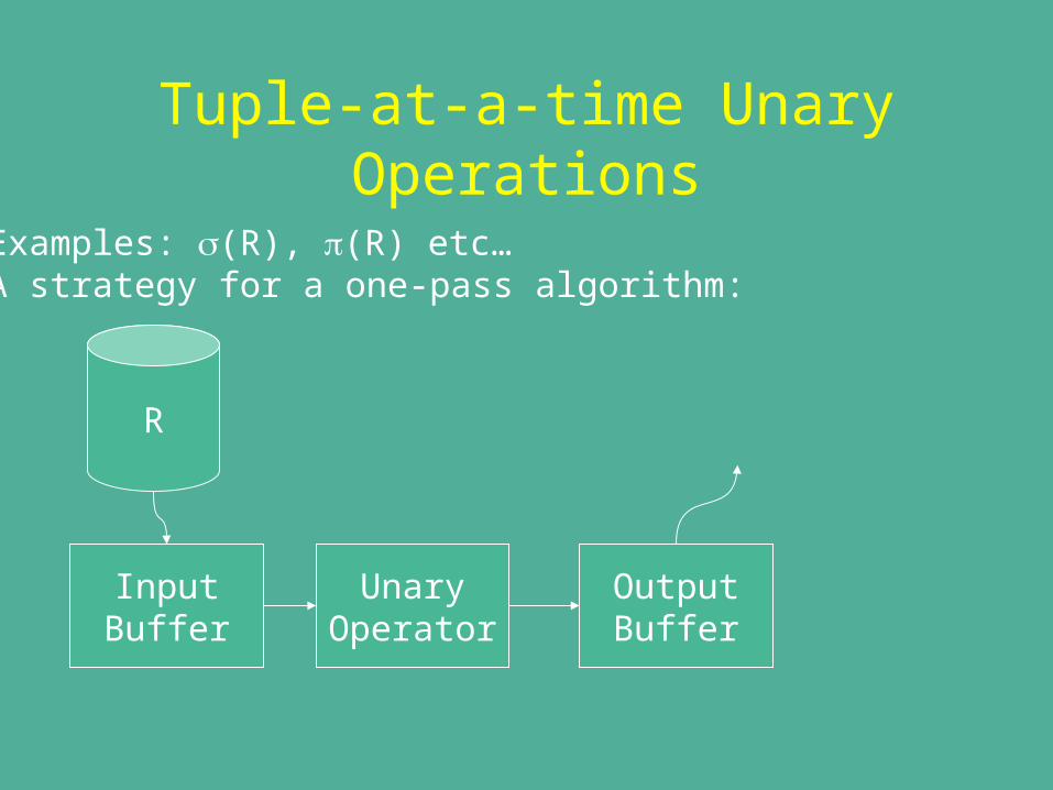
Tuple-at-a-time Unary Operations
Examples: (R), (R) etc…A strategy for a one-pass algorithm:
R
InputBuffer
UnaryOperator
OutputBuffer
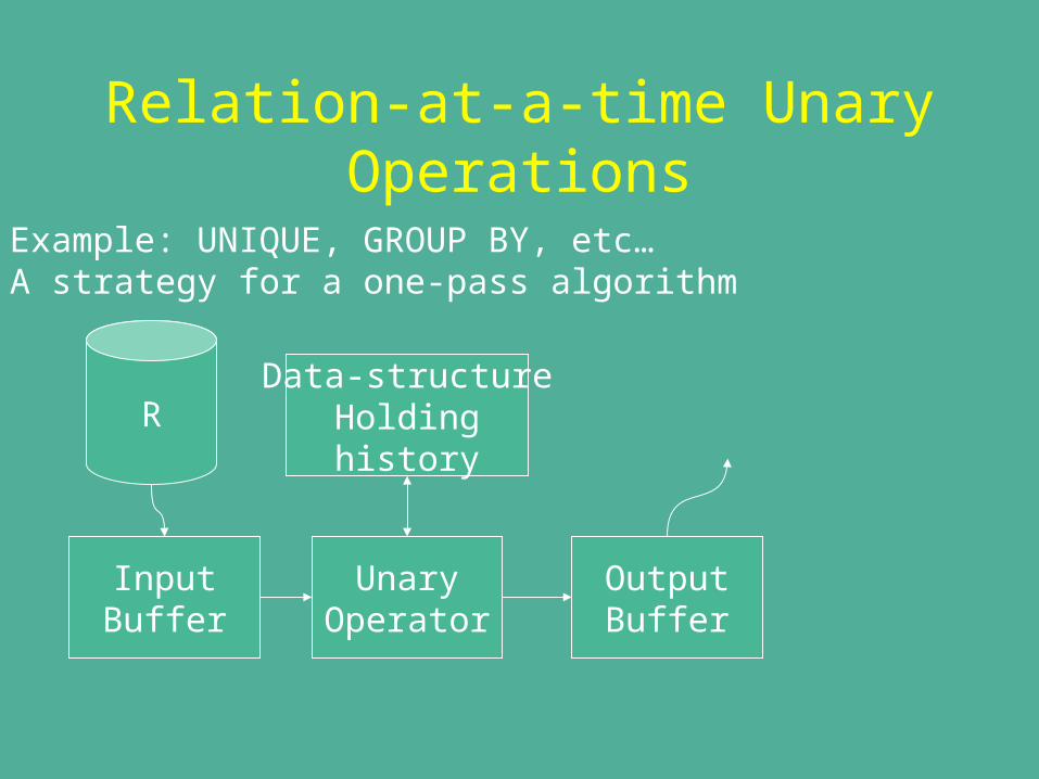
Relation-at-a-time Unary Operations
Example: UNIQUE, GROUP BY, etc…A strategy for a one-pass algorithm
R
InputBuffer
UnaryOperator
OutputBuffer
Data-structureHoldinghistory
Relation-at-a-time Binary Operators
One-pass strategies for binary relation-at-a-time operators vary between different operators.
Almost all of them require at least one of the relation to be completely stored in memory.
Strategies
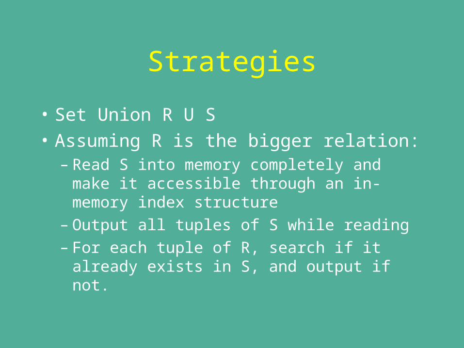
• Set Union R U S
• Assuming R is the bigger relation: – Read S into memory completely and make
it accessible through an in-memory index structure
– Output all tuples of S while reading– For each tuple of R, search if it already
exists in S, and output if not.
Strategies
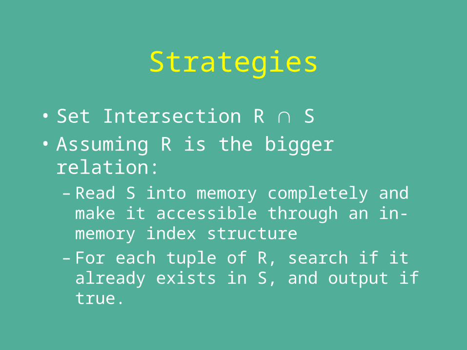
• Set Intersection R S
• Assuming R is the bigger relation: – Read S into memory completely and make
it accessible through an in-memory index structure
– For each tuple of R, search if it already exists in S, and output if true.
Strategies
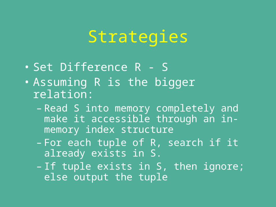
• Set Difference R - S• Assuming R is the bigger relation:
– Read S into memory completely and make it accessible through an in-memory index structure
– For each tuple of R, search if it already exists in S.
– If tuple exists in S, then ignore; else output the tuple
Strategies
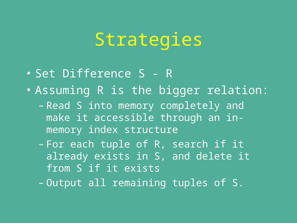
• Set Difference S - R
• Assuming R is the bigger relation: – Read S into memory completely and make
it accessible through an in-memory index structure
– For each tuple of R, search if it already exists in S, and delete it from S if it exists
– Output all remaining tuples of S.
Strategies
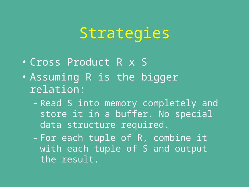
• Cross Product R x S
• Assuming R is the bigger relation: – Read S into memory completely and store
it in a buffer. No special data structure required.
– For each tuple of R, combine it with each tuple of S and output the result.

Strategies
• Natural Join R * S. Assume R(X,Y) and S(Y,Z)
• Assuming R is the bigger relation: – Read S into memory completely and store
it in an balanced tree index structure or a hash table.
– For each tuple of R, search S to see if a matching tuple exists.
– Output if matching tuple found.
One-pass algorithms
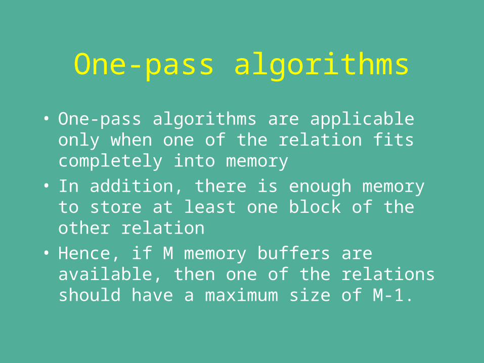
• One-pass algorithms are applicable only when one of the relation fits completely into memory
• In addition, there is enough memory to store at least one block of the other relation
• Hence, if M memory buffers are available, then one of the relations should have a maximum size of M-1.

One-pass Algorithms
• One pass algorithms rely on correctly estimating relation sizes and allocating memory buffers
• If too many buffers are allocated, there is a possibility of thrashing
• If too few buffers are allocated, then one-pass algorithms may not run
Summary
• Stages in Query Processing• Logical Query Plan and Physical Query
Plan• Intermediate Query Language • Physical Query Plan language
constructs• One-pass algorithms for unary and
binary operators.
Query Processing and Optimization (contd.)

Query Processing
• Efficient Query Processing crucial for good or even effective operations of a database
• Query Processing depends on a variety of factors, not everything under the control of the DBMS
• Insufficient or incorrect information can result in vastly ineffective plans
• Query Cataloging
Steps in Query Execution
SQL QueryScanning,Parsing,
Validating
Intermediate query representation (logical query plan tree)

Steps in Query Execution
IntermediateQueryRepresentation
QueryOptimizer
Query Execution Plan(physical query plan tree)
Steps in Query Execution
Query ExecutionPlan
QueryCode
Generator
Code to execute query
Steps in Query Execution
Code to ExecuteQuery
Run-timeDatabaseProcessor
Query Results

Query Processing
• Intermediate Form– Usually a relational algebra form of the
SQL query – Uses heuristics and cost-based measures
for optimization
• Physical Query Plan– In a language that is interpreted and
executed on the machine or compiled into machine code.
Physical-Query-Plan Operators
• Basic set of operators that define the language of physical query execution plans
• Comprises the set of relational operators in addition to some more required operators
• Example operators: Table-scan, Index-scan, Sort-scan, Iterator, etc…

One-pass Algorithms
• One-pass algorithms are applicable only when one of the relation fits completely into memory
• In addition, there is enough memory to store at least one block of the other relation
• Hence, if M memory buffers are available, then one of the relations should have a maximum size of M-1.
One-pass Algorithms
• One pass algorithms rely on correctly estimating relation sizes and allocating memory buffers
• If too many buffers are allocated, there is a possibility of thrashing
• If too few buffers are allocated, then one-pass algorithms may not run
Multi-pass Algorithms
• Used when entire relations cannot be read into memory
• Requires alternate computation and retrieval of intermediate results
• Many multi-pass algorithms are generalizations of their corresponding two pass algorithms
Basic Idea: Two-pass Algorithms Based on Sorting
• Suppose relation R is too big to fit in memory which can accommodate only M blocks of data.
• The “sorting-based” 2-pass algorithms have the following basic structure:
Basic Idea: Two-pass Algorithms Based on Sorting
1. Read M blocks of records into memory and sort them
2. Write them back to disk 3. Continue steps 1 and 2 until R is
exhausted4. Use a variety of “query-merge”
techniques to extract relevant results from all the sorted M-blocks on disk.
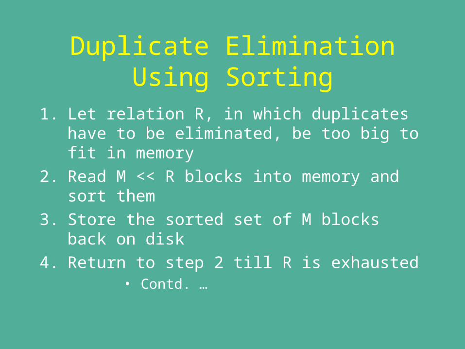
Duplicate Elimination Using Sorting
1. Let relation R, in which duplicates have to be eliminated, be too big to fit in memory
2. Read M << R blocks into memory and sort them
3. Store the sorted set of M blocks back on disk
4. Return to step 2 till R is exhausted• Contd. …
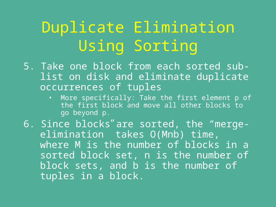
Duplicate Elimination Using Sorting
5. Take one block from each sorted sub-list on disk and eliminate duplicate occurrences of tuples
• More specifically: Take the first element p of the first block and move all other blocks to go beyond p.
6. Since blocks are sorted, the “merge-elimination” takes O(Mnb) time, where M is the number of blocks in a sorted block set, n is the number of block sets, and b is the number of tuples in a block.
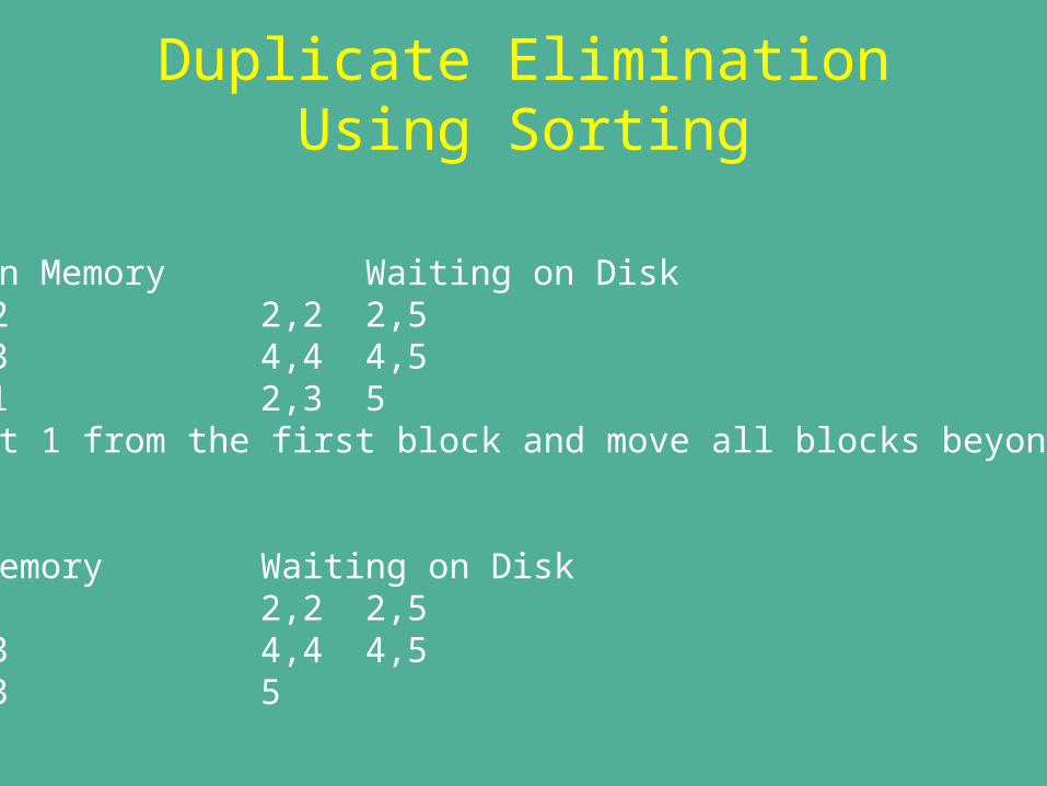
Duplicate Elimination Using Sorting
In Memory Waiting on Disk1 1,2 2,2 2,52 2,3 4,4 4,53 1,1 2,3 5 Output 1 from the first block and move all blocks beyond “1”.
In Memory Waiting on Disk1 2 2,2 2,52 2,3 4,4 4,53 2,3 5
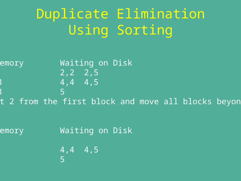
Duplicate Elimination Using Sorting
In Memory Waiting on Disk1 2 2,2 2,52 2,3 4,4 4,53 2,3 5 Output 2 from the first block and move all blocks beyond “2”.
In Memory Waiting on Disk1 52 3 4,4 4,53 3 5
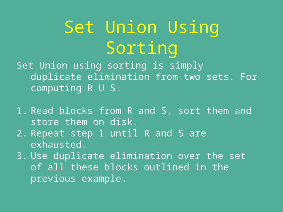
Set Union Using Sorting
Set Union using sorting is simply duplicate elimination from two sets. For computing R U S:
1. Read blocks from R and S, sort them and store them on disk.
2. Repeat step 1 until R and S are exhausted. 3. Use duplicate elimination over the set of all these
blocks outlined in the previous example.
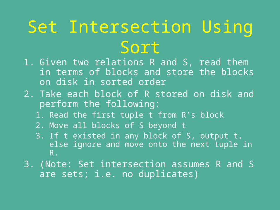
Set Intersection Using Sort1. Given two relations R and S, read them in
terms of blocks and store the blocks on disk in sorted order
2. Take each block of R stored on disk and perform the following:
1. Read the first tuple t from R’s block2. Move all blocks of S beyond t 3. If t existed in any block of S, output t, else ignore
and move onto the next tuple in R.
3. (Note: Set intersection assumes R and S are sets; i.e. no duplicates)
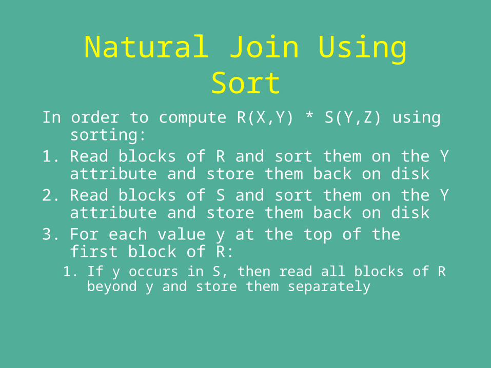
Natural Join Using Sort
In order to compute R(X,Y) * S(Y,Z) using sorting:
1. Read blocks of R and sort them on the Y attribute and store them back on disk
2. Read blocks of S and sort them on the Y attribute and store them back on disk
3. For each value y at the top of the first block of R:
1. If y occurs in S, then read all blocks of R beyond y and store them separately
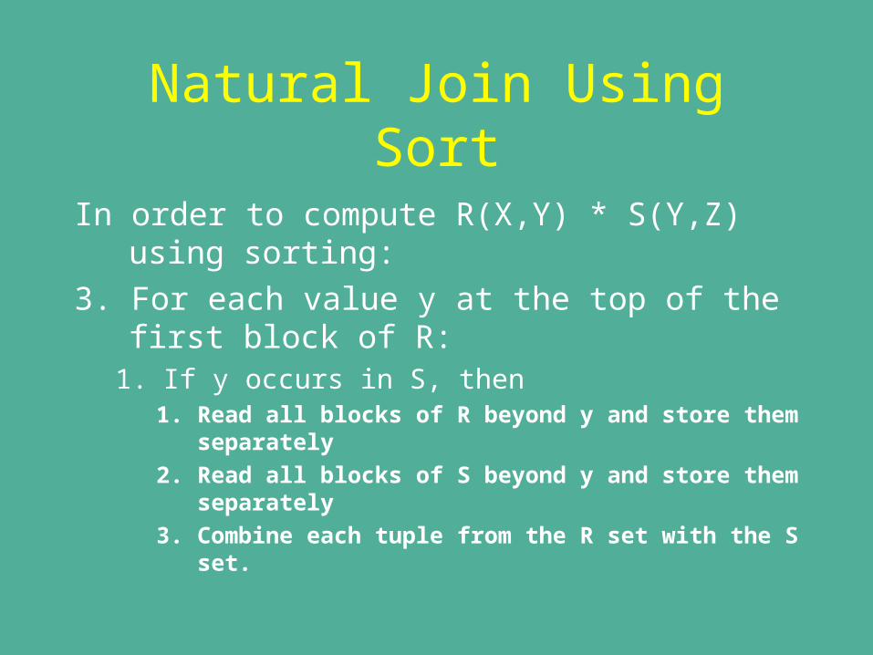
Natural Join Using Sort
In order to compute R(X,Y) * S(Y,Z) using sorting:
3. For each value y at the top of the first block of R:
1. If y occurs in S, then 1. Read all blocks of R beyond y and store them
separately
2. Read all blocks of S beyond y and store them separately
3. Combine each tuple from the R set with the S set.
Hash Based Algorithms
• Basic Idea:1. Read relation R block by block
2. Take each tuple in a block and hash it to one of a set of buckets of a hash file
3. All “similar” tuples should hash to the same bucket
4. Examine each bucket in isolation to produce final result.
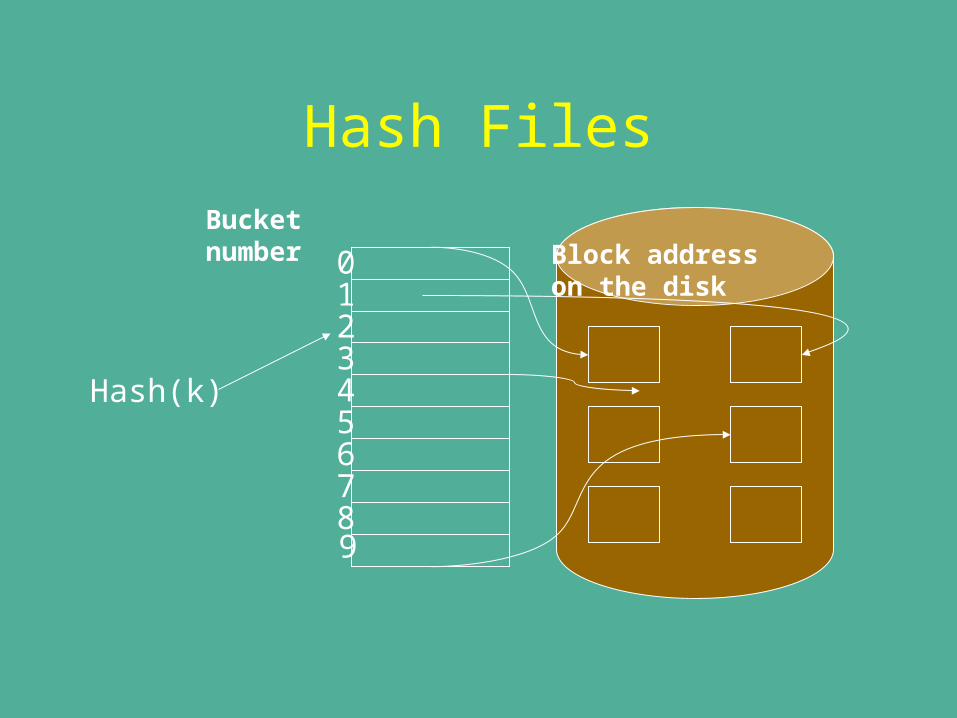
Hash Files
0
456789
23
1
Bucketnumber Block address
on the disk
Hash(k)
Hash Based Duplicate Elimination
• Eliminate duplicates from relation R that is too big to fit in memory:
1. Read relation R block by block
2. Take each tuple in a block and hash it to one of a set of buckets of a hash file. Note that duplicate tuples hash to the same bucket
3. Visit each bucket and eliminate duplicates using either a one-pass algorithm (if bucket fits in memory) or a two-pass sort based algorithm (if bucket too big to fit in memory).

Hash Based Set Operations
• For set operations involving two relations R and S, two separate hash files are maintained.
• However the same hash function is used and buckets in the two hash files are numbered analogously
• If tuple t appears in bucket # n in R’s hash file, then t, if it is present in S, should also appear in bucket # n in S’s hash file.
• In addition, all duplicate tuples are hashed to the same bucket of a given hash file.
Hash Based Set Operations
• Read relation R block by block and hash every tuple to R’s hash file
• Read relation S block by block and hash every tuple to S’s hash file
• Read corresponding buckets from R’s and S’s hash file to perform set union, intersection and difference.
The Hash-Join Algorithm• Natural Join over relations R(X,Y) and S(Y,Z) is
achieved by hashing using just the Y component of R and S
• All tuples having the same value of the Y component should hash to the same bucket
• If same hash function is used for R and S, corresponding buckets can be compared
• Use a one-pass join algorithm by using corresponding buckets from the hash files of R and S.
• Above algorithm sometimes termed “partition hash-join” algorithm
Index Based Algorithms
• Useful when tuples have to be extracted from relations based on attributes that have been indexed
• Especially useful for selection functions• Fairly effective for joins and other binary
operations• Primary indexes in the following
examples are assumed to be B+ trees.
Index Based Selection
• Straightforward if selection is an equality condition on an indexed attribute (a =10).
• Simply search the index for the required set of tuple(s).
• In case of inequality conditions (a<=10), tuples have to be retrieved from a sub tree that matches the condition.
Index-Based Natural Joins
• Consider natural join between R(X,Y) and S(Y,Z). Assume that S has an index over its Y component. – Read R block by block– For each tuple in the block, extract its Y
component and search relation S based on the Y component
– If a corresponding tuple is found, perform the join and append to output buffer.
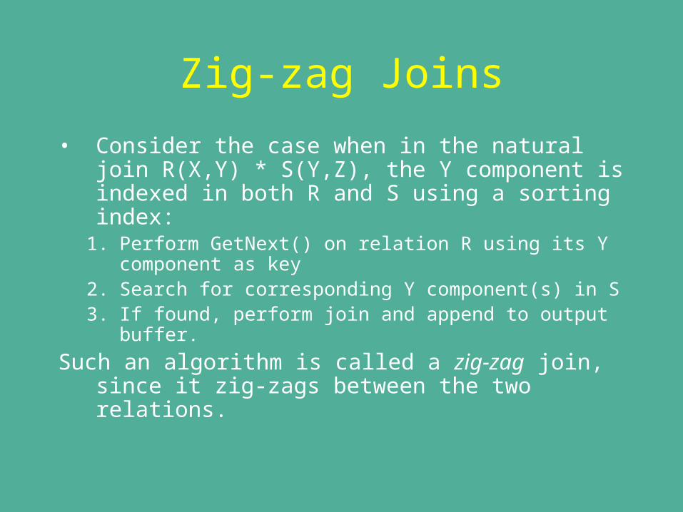
Zig-zag Joins
• Consider the case when in the natural join R(X,Y) * S(Y,Z), the Y component is indexed in both R and S using a sorting index:
1. Perform GetNext() on relation R using its Y component as key
2. Search for corresponding Y component(s) in S3. If found, perform join and append to output buffer.
Such an algorithm is called a zig-zag join, since it zig-zags between the two relations.
Summary of Query Processing
• Different Stages of Query Execution• Physical-Query-Plan Language• Iterators• Single-pass Algorithms and their limitations• Multi-pass algorithms• Sort based algorithms• Hash based algorithms• Index based algorithms

Query Optimization
Steps in Query Processing
• Scanning and Parsing
• Logical Query Plan generation
• Query rewriting (optimization)
• Physical Query Plan generation
• Code generation / query execution
Database Access Algorithms
Algorithms for database access can be broadly divided in the following categories:
– Sorting-based methods – Hash-based methods– Index-based methods

Index Based Algorithms
• Useful when tuples have to be extracted from relations based on attributes that have been indexed
• Especially useful for selection functions• Fairly effective for joins and other binary
operations• Primary indexes in the following
examples are assumed to be B+ trees.
Query Optimization
• Based on rewriting Parse Tree representing a relational algebra expression of the query
• Heuristics based optimization versus Cost-based optimization
Parse TreesSyntactic structures of most programming languages can be expressed in the form of a “syntax tree” also called the “parse tree”.
Execution of a syntactic construct can be achieved by a “post-order traversal” of a parse tree.
Parse Trees
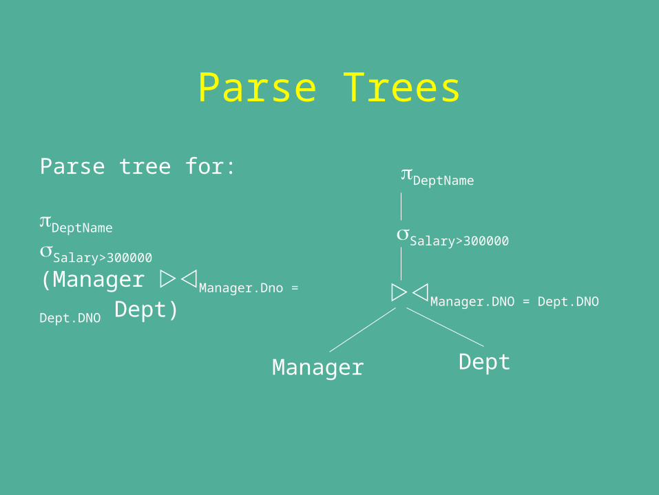
Parse tree for:
DeptName
Salary>300000 (Manager Manager.Dno = Dept.DNO Dept)
DeptName
Salary>300000
Manager.DNO = Dept.DNO
Manager Dept
Checks on Parse Trees
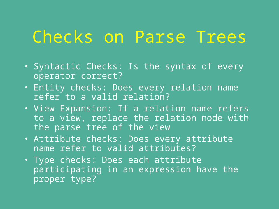
• Syntactic Checks: Is the syntax of every operator correct?
• Entity checks: Does every relation name refer to a valid relation?
• View Expansion: If a relation name refers to a view, replace the relation node with the parse tree of the view
• Attribute checks: Does every attribute name refer to valid attributes?
• Type checks: Does each attribute participating in an expression have the proper type?
Rewriting Parse Trees
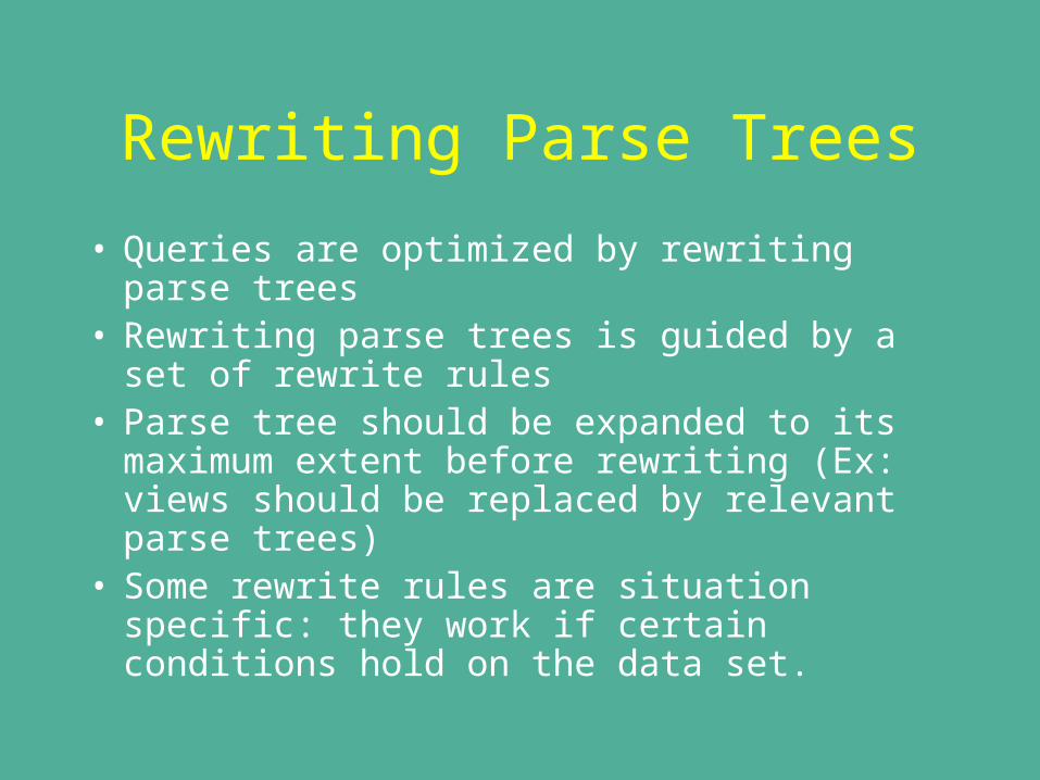
• Queries are optimized by rewriting parse trees
• Rewriting parse trees is guided by a set of rewrite rules
• Parse tree should be expanded to its maximum extent before rewriting (Ex: views should be replaced by relevant parse trees)
• Some rewrite rules are situation specific: they work if certain conditions hold on the data set.
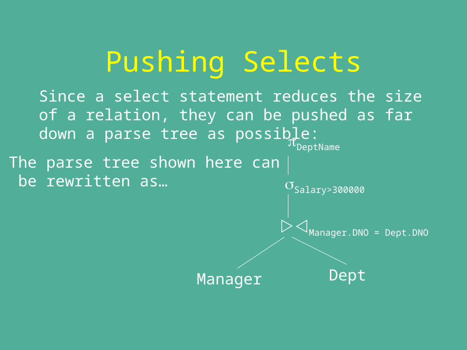
Pushing SelectsSince a select statement reduces the size of a relation, they can be pushed as far down a parse tree as possible:
DeptName
Salary>300000
Manager.DNO = Dept.DNO
Manager Dept
The parse tree shown here can be rewritten as…
Pushing Selects
DeptName
Salary>300000
Manager.DNO = Dept.DNO
Manager
Dept
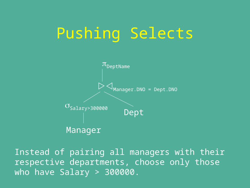
Instead of pairing all managers with their respective departments, choose only those who have Salary > 300000.
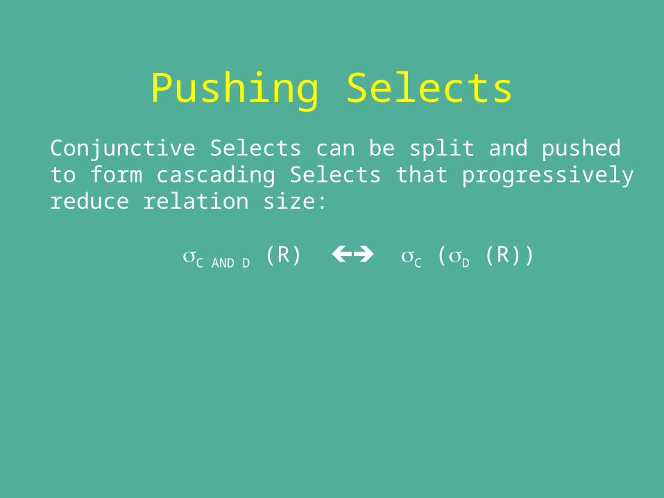
Pushing SelectsConjunctive Selects can be split and pushed to form cascading Selects that progressively reduce relation size:
C AND D (R) C (D (R))
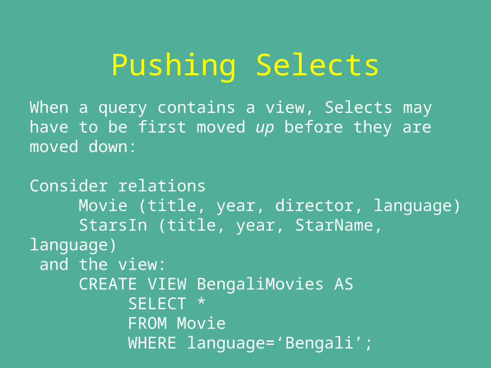
Pushing SelectsWhen a query contains a view, Selects may have to be first moved up before they are moved down: Consider relations
Movie (title, year, director, language)StarsIn (title, year, StarName, language)
and the view: CREATE VIEW BengaliMovies AS
SELECT * FROM MovieWHERE language=‘Bengali’;
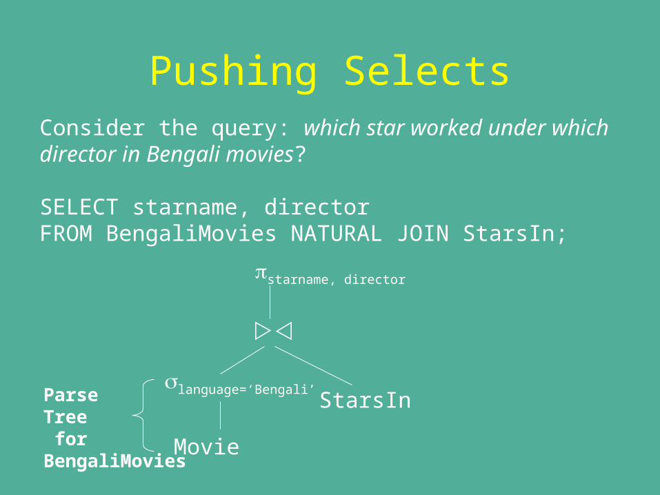
Pushing SelectsConsider the query: which star worked under which director in Bengali movies?
SELECT starname, director FROM BengaliMovies NATURAL JOIN StarsIn;
starname, director
language=‘Bengali’
Movie
StarsInParseTree forBengaliMovies
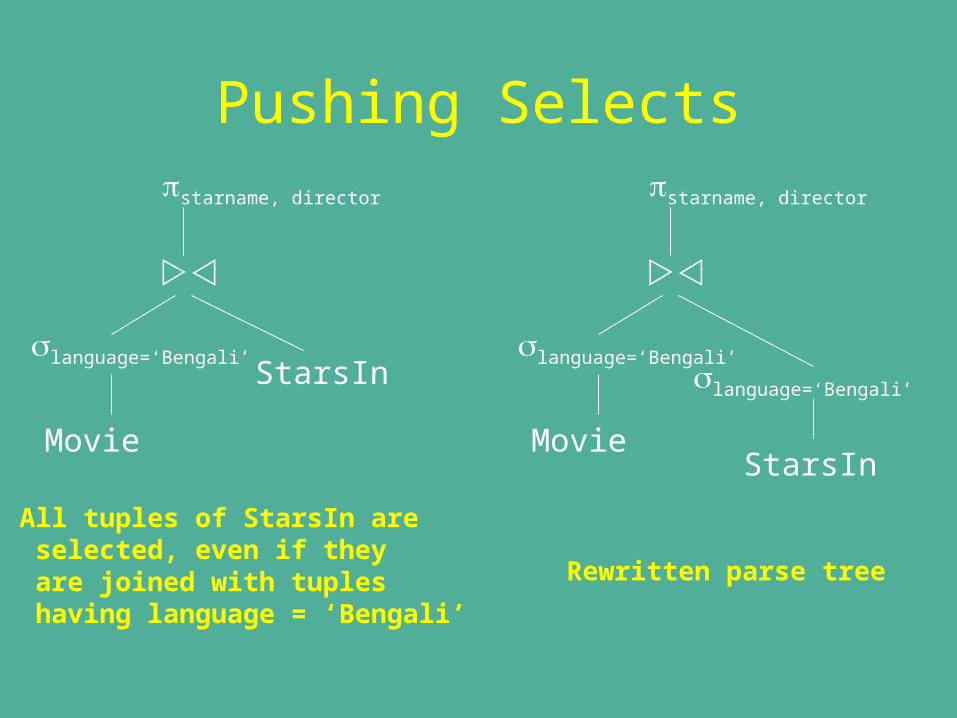
Pushing Selectsstarname, director
language=‘Bengali’
Movie
StarsIn
All tuples of StarsIn are selected, even if they are joined with tuples having language = ‘Bengali’
starname, director
language=‘Bengali’
MovieStarsIn
language=‘Bengali’
Rewritten parse tree
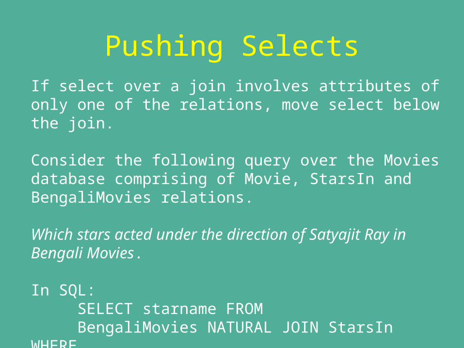
Pushing SelectsIf select over a join involves attributes of only one of the relations, move select below the join.
Consider the following query over the Movies database comprising of Movie, StarsIn and BengaliMovies relations.
Which stars acted under the direction of Satyajit Ray in Bengali Movies.
In SQL: SELECT starname FROM BengaliMovies NATURAL JOIN StarsIn WHERE director = ‘Satyajit Ray’
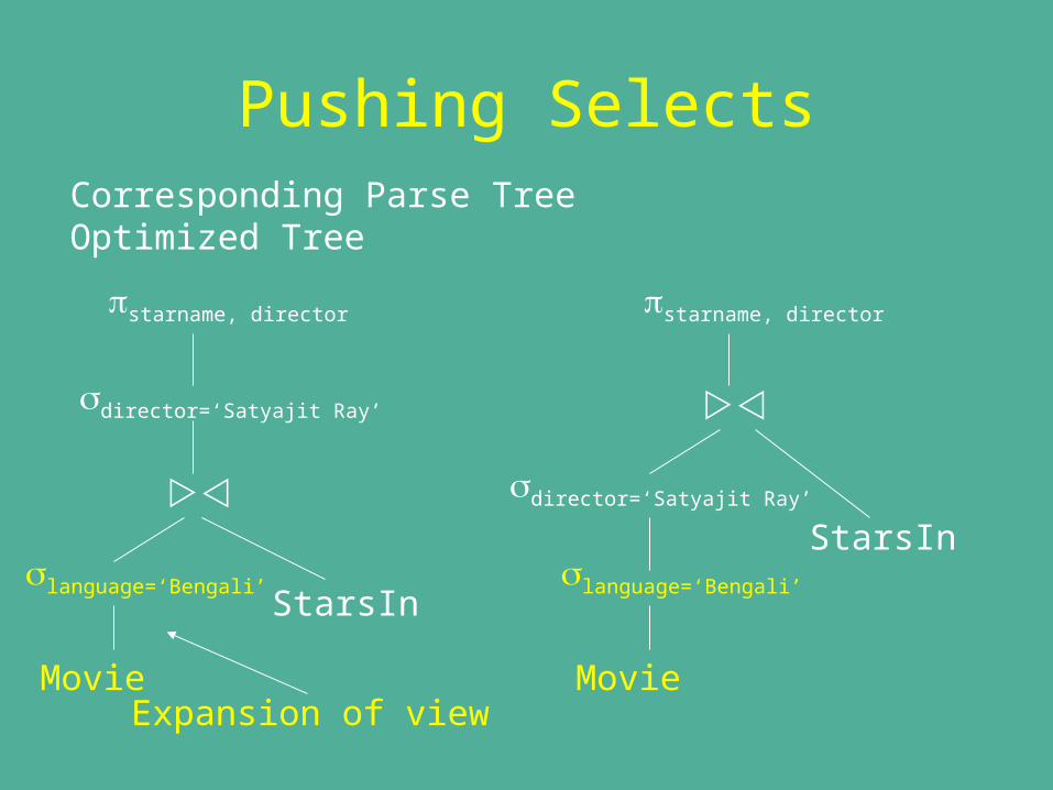
Pushing SelectsCorresponding Parse Tree Optimized Tree
starname, director
language=‘Bengali’
Movie
StarsIn
director=‘Satyajit Ray’
Expansion of view
starname, director
language=‘Bengali’
Movie
StarsIn
director=‘Satyajit Ray’
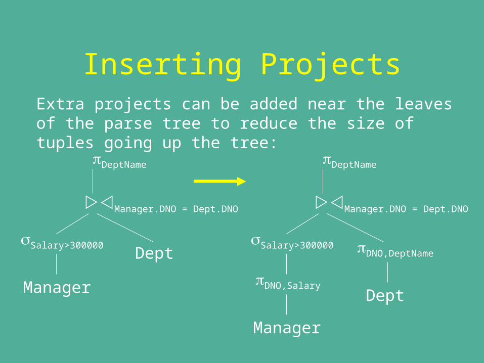
Inserting ProjectsExtra projects can be added near the leaves of the parse tree to reduce the size of tuples going up the tree:
DeptName
Salary>300000
Manager.DNO = Dept.DNO
Manager
Dept
DeptName
Salary>300000
Manager.DNO = Dept.DNO
Manager
DeptDNO,Salary
DNO,DeptName
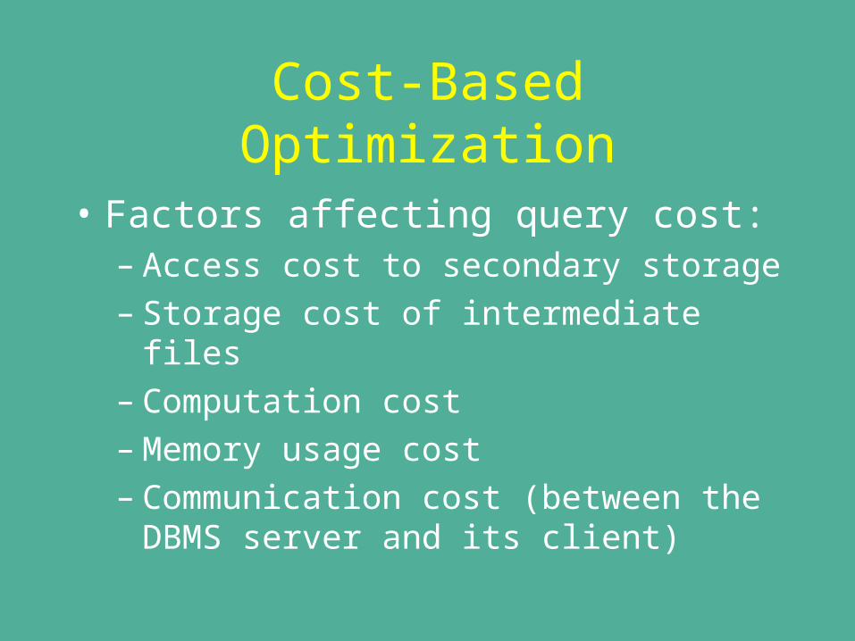
Cost-Based Optimization
• Factors affecting query cost: – Access cost to secondary storage– Storage cost of intermediate files – Computation cost– Memory usage cost– Communication cost (between the DBMS
server and its client)
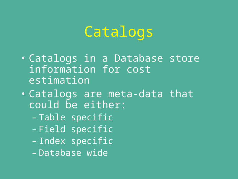
Catalogs
• Catalogs in a Database store information for cost estimation
• Catalogs are meta-data that could be either: – Table specific – Field specific– Index specific– Database wide
Catalog Examples
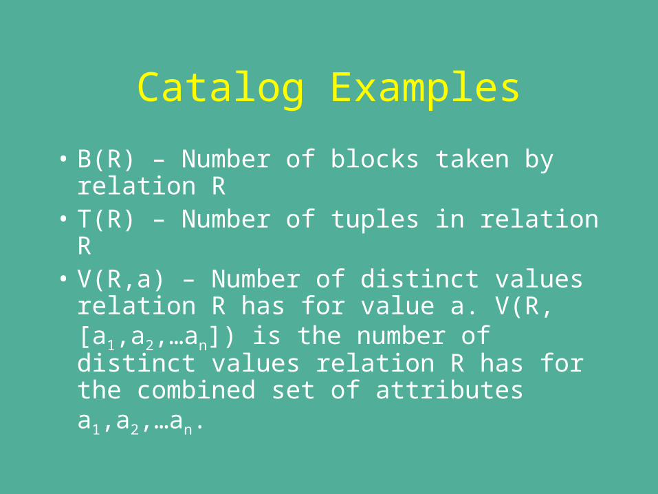
• B(R) – Number of blocks taken by relation R
• T(R) – Number of tuples in relation R • V(R,a) – Number of distinct values
relation R has for value a. V(R, [a1,a2,…an]) is the number of distinct values relation R has for the combined set of attributes a1,a2,…an.
Cost Estimation Examples
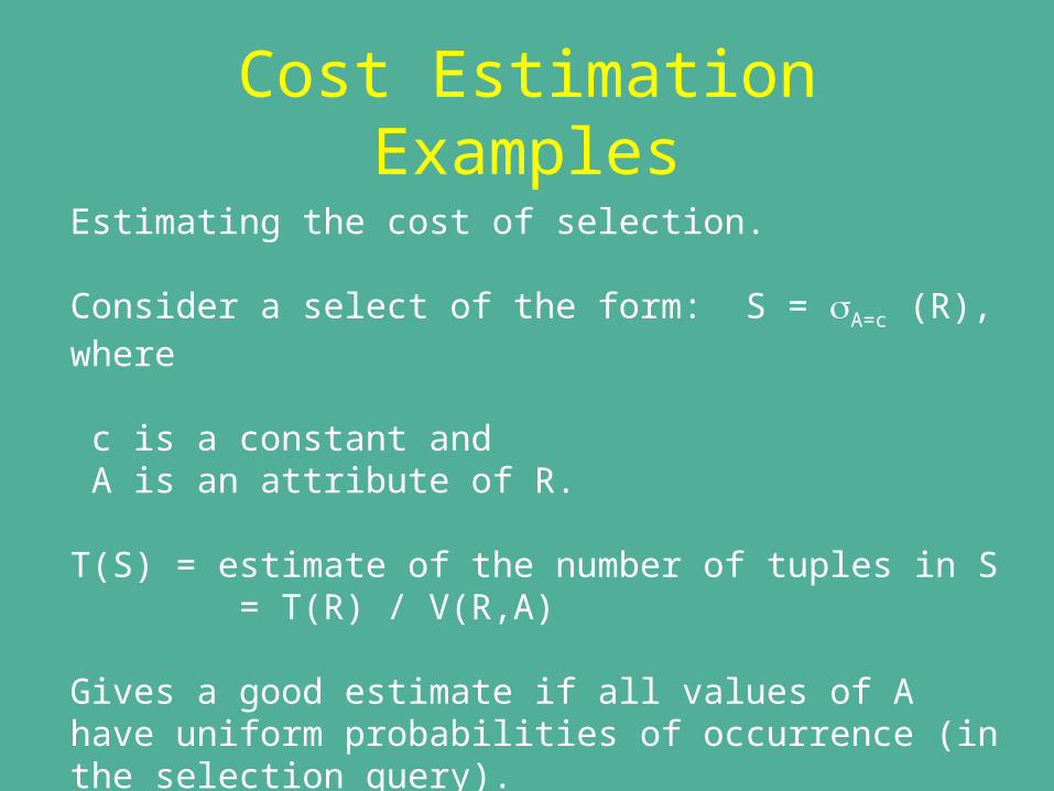
Estimating the cost of selection.
Consider a select of the form: S = A=c (R), where
c is a constant and A is an attribute of R.
T(S) = estimate of the number of tuples in S = T(R) / V(R,A)
Gives a good estimate if all values of A have uniform probabilities of occurrence (in the selection query).
Cost Estimation Examples
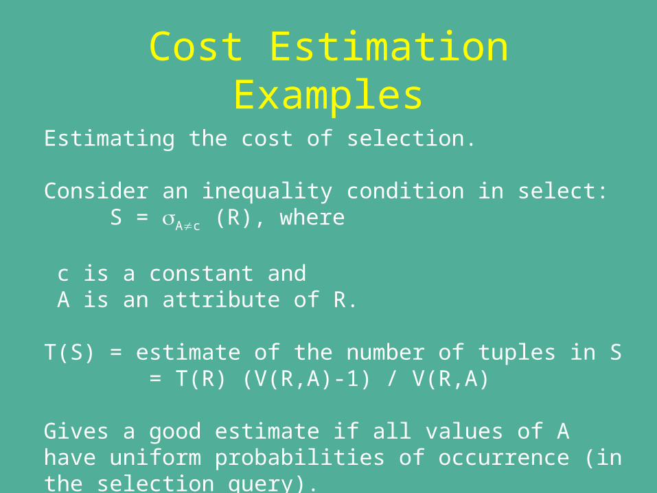
Estimating the cost of selection.
Consider an inequality condition in select: S = Ac (R), where
c is a constant and A is an attribute of R.
T(S) = estimate of the number of tuples in S = T(R) (V(R,A)-1) / V(R,A)
Gives a good estimate if all values of A have uniform probabilities of occurrence (in the selection query).
Cost Estimation Examples
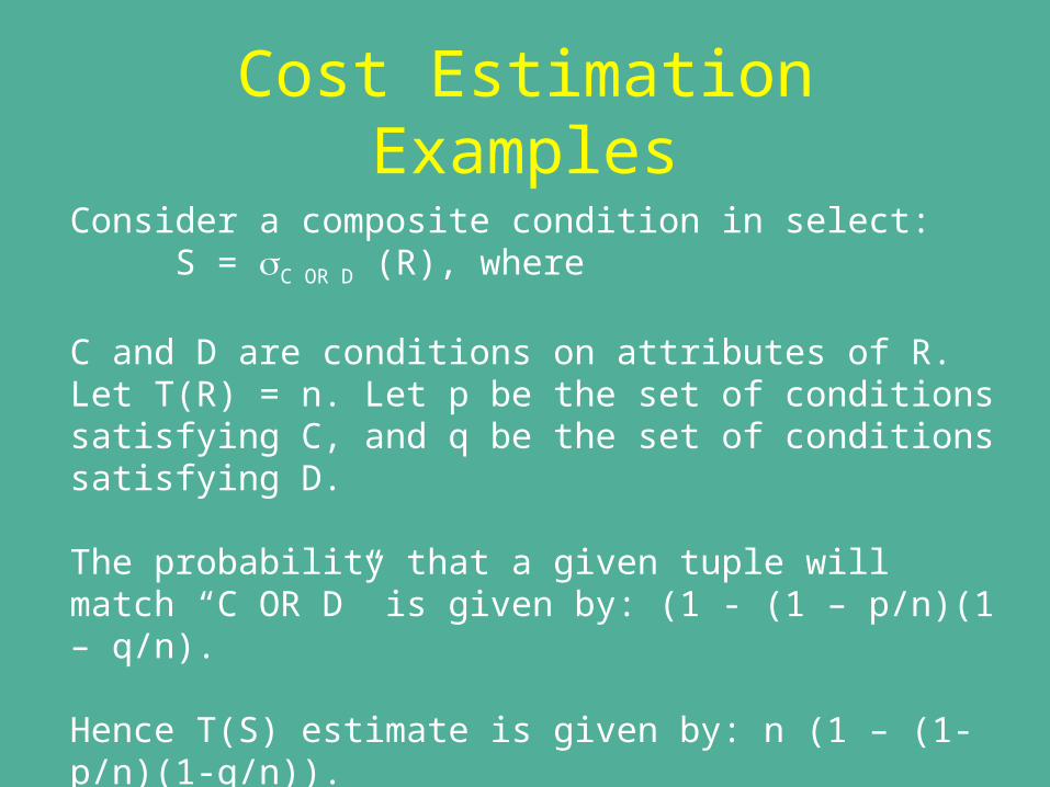
Consider a composite condition in select: S = C OR D (R), where
C and D are conditions on attributes of R. Let T(R) = n. Let p be the set of conditions satisfying C, and q be the set of conditions satisfying D.
The probability that a given tuple will match “C OR D” is given by: (1 - (1 – p/n)(1 – q/n).
Hence T(S) estimate is given by: n (1 – (1-p/n)(1-q/n)).
Estimating size of natural joins
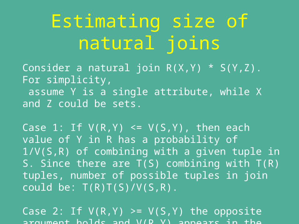
Consider a natural join R(X,Y) * S(Y,Z). For simplicity, assume Y is a single attribute, while X and Z could be sets.
Case 1: If V(R,Y) <= V(S,Y), then each value of Y in R has a probability of 1/V(S,R) of combining with a given tuple in S. Since there are T(S) combining with T(R) tuples, number of possible tuples in join could be: T(R)T(S)/V(S,R).
Case 2: If V(R,Y) >= V(S,Y) the opposite argument holds and V(R,Y) appears in the denominator.
Estimating size of natural joins
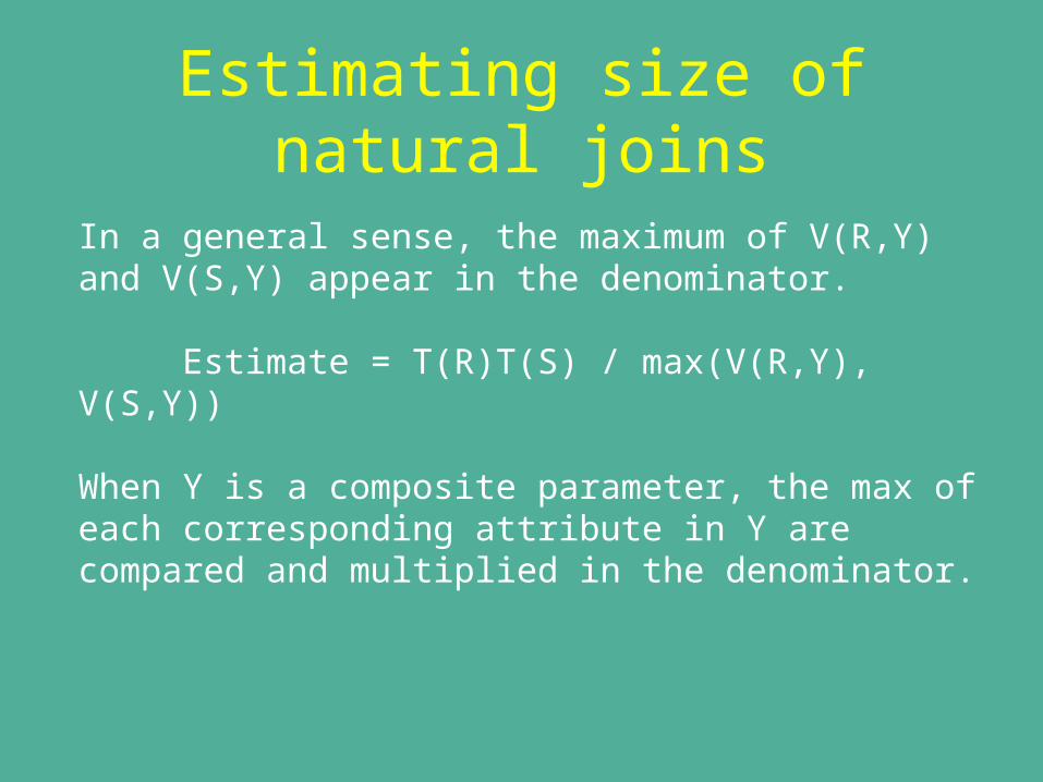
In a general sense, the maximum of V(R,Y) and V(S,Y) appear in the denominator.
Estimate = T(R)T(S) / max(V(R,Y), V(S,Y))
When Y is a composite parameter, the max of each corresponding attribute in Y are compared and multiplied in the denominator.
Summary
• Index Based Algorithms• Query Optimization by rewriting parse tree
– Pushing selects– Cascading selects– Pulling selects from views– Extra projects
• Cost estimation of query components based on catalog information