Query Optimization Techniques for Partitioned Tables

Herodotos HerodotouDuke University

Durham, North Carolina, USAhero@cs.duke.edu

Nedyalko BorisovDuke University

Durham, North Carolina, USAnedyalko@cs.duke.edu

Shivnath Babu∗

Duke UniversityDurham, North Carolina, USAshivnath@cs.duke.edu

ABSTRACTTable partitioning splits a table into smaller parts that can be ac-cessed, stored, and maintained independent of one another. Fromtheir traditional use in improving query performance, partitioningstrategies have evolved into a powerful mechanism to improve theoverall manageability of database systems. Table partitioning sim-plifies administrative tasks like data loading, removal, backup, statis-tics maintenance, and storage provisioning. Query language exten-sions now enable applications and user queries to specify how theirresults should be partitioned for further use. However, query opti-mization techniques have not kept pace with the rapid advances inusage and user control of table partitioning. We address this gapby developing new techniques to generate efficient plans for SQLqueries involving multiway joins over partitioned tables. Our tech-niques are designed for easy incorporation into bottom-up queryoptimizers that are in wide use today. We have prototyped thesetechniques in the PostgreSQL optimizer. An extensive evaluationshows that our partition-aware optimization techniques, with lowoptimization overhead, generate plans that can be an order of mag-nitude better than plans produced by current optimizers.

Categories and Subject DescriptorsH.2.4 [Database Management]: Systems—query processing

General TermsAlgorithms

Keywordsquery optimization, partitioning

1. INTRODUCTIONTable partitioning is a standard feature in database systems today

[13, 15, 20, 21]. For example, a sales records table may be parti-tioned horizontally based on value ranges of a date column. Onepartition may contain all sales records for the month of January,∗Supported by NSF grants 0964560 and 0917062

Permission to make digital or hard copies of all or part of this work forpersonal or classroom use is granted without fee provided that copies arenot made or distributed for profit or commercial advantage and that copiesbear this notice and the full citation on the first page. To copy otherwise, torepublish, to post on servers or to redistribute to lists, requires prior specificpermission and/or a fee.SIGMOD’11, June 12–16, 2011, Athens, Greece.Copyright 2011 ACM 978-1-4503-0661-4/11/06 ...$10.00.

Uses of Table Partitioning in Database SystemsEfficient pruning of unneeded data during query processingParallel data access (partitioned parallelism) during query processingReducing data contention during query processing and administrativetasks. Faster data loading, archival, and backupEfficient statistics maintenance in response to insert, delete, and updaterates. Better cardinality estimation for subplans that access few partitionsPrioritized data storage on faster/slower disks based on access patternsFine-grained control over physical design for database tuningEfficient and online table and index defragmentation at the partition level

Table 1: Uses of table partitioning in database systemsanother partition may contain all sales records for February, and soon. A table can also be partitioned vertically with each partitioncontaining a subset of columns in the table. Hierarchical combina-tions of horizontal and vertical partitioning may also be used.

The trend of rapidly growing data sizes has amplified the usageof partitioned tables in database systems. Table 1 lists various usesof table partitioning. Apart from giving major performance im-provements, partitioning simplifies a number of common adminis-trative tasks in database systems. In this paper, we focus on hori-zontal table partitioning in centralized row-store database systemssuch as those sold by major database vendors as well as popularopen-source systems like MySQL and PostgreSQL. The uses of ta-ble partitioning in these systems have been studied [2, 24].

The growing usage of table partitioning has been accompaniedby efforts to give applications and users the ability to specify parti-tioning conditions for tables that they derive from base data. SQLextensions from database vendors now enable queries to specifyhow derived tables are partitioned (e.g., [11]). Given such exten-sions, Database Administrators (DBAs) may not be able to con-trol or restrict how tables accessed in a query are partitioned. Fur-thermore, multiple objectives—e.g., getting fast data loading alongwith good query performance—and constraints—e.g., on the max-imum size or number of partitions per table—may need to be metwhile choosing how each table in the database is partitioned.

1.1 Query Optimization for Partitioned TablesQuery optimization technology has not kept pace with the grow-

ing usage and user control of table partitioning. Previously, queryoptimizers had to consider only the restricted partitioning schemesspecified by the DBA on base tables. Today, the optimizer facesa diverse mix of partitioning schemes that expand on traditionalschemes like hash and equi-range partitioning. Hierarchical (ormultidimensional) partitioning is one such scheme to deal with mul-tiple granularities or hierarchies in the data [4]. A table is first par-titioned on one attribute. Each partition is further partitioned on adifferent attribute; and so on for two or more levels.

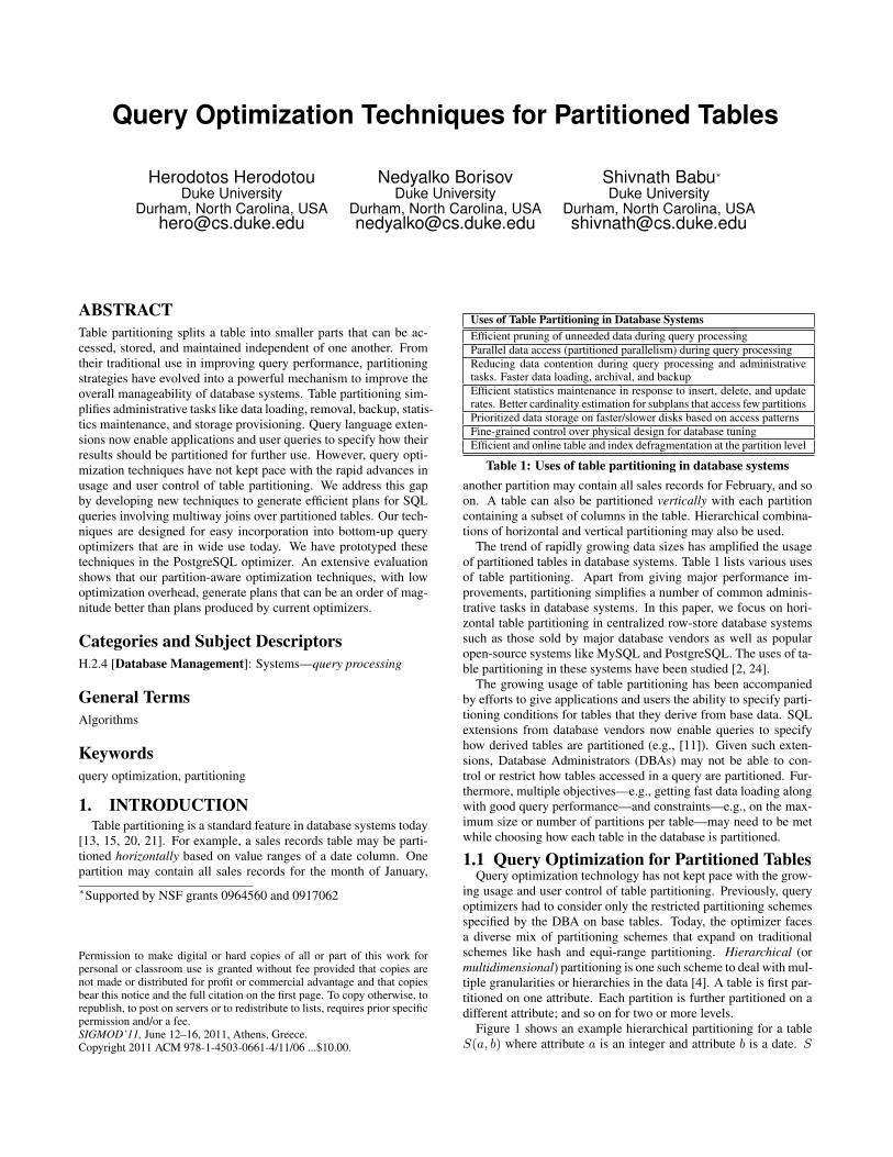
Figure 1 shows an example hierarchical partitioning for a tableS(a, b) where attribute a is an integer and attribute b is a date. S

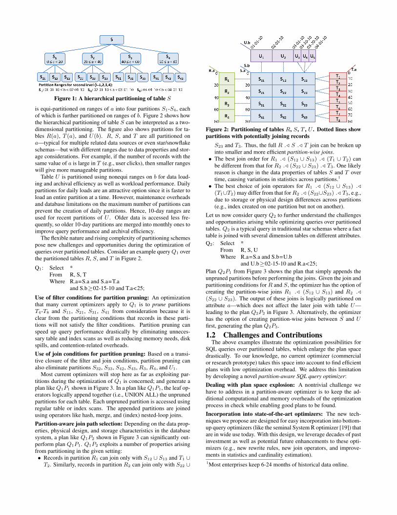
Figure 1: A hierarchical partitioning of table S

is equi-partitioned on ranges of a into four partitions S1-S4, eachof which is further partitioned on ranges of b. Figure 2 shows howthe hierarchical partitioning of table S can be interpreted as a two-dimensional partitioning. The figure also shows partitions for ta-bles R(a), T (a), and U(b). R, S, and T are all partitioned ona—typical for multiple related data sources or even star/snowflakeschemas—but with different ranges due to data properties and stor-age considerations. For example, if the number of records with thesame value of a is large in T (e.g., user clicks), then smaller rangeswill give more manageable partitions.

Table U is partitioned using nonequi ranges on b for data load-ing and archival efficiency as well as workload performance. Dailypartitions for daily loads are an attractive option since it is faster toload an entire partition at a time. However, maintenance overheadsand database limitations on the maximum number of partitions canprevent the creation of daily partitions. Hence, 10-day ranges areused for recent partitions of U . Older data is accessed less fre-quently, so older 10-day partitions are merged into monthly ones toimprove query performance and archival efficiency.

The flexible nature and rising complexity of partitioning schemespose new challenges and opportunities during the optimization ofqueries over partitioned tables. Consider an example queryQ1 overthe partitioned tables R, S, and T in Figure 2.

Q1: Select *From R, S, TWhere R.a=S.a and S.a=T.a

and S.b≥02-15-10 and T.a<25;

Use of filter conditions for partition pruning: An optimizationthat many current optimizers apply to Q1 is to prune partitionsT4-T8 and S11, S21, S31, S41 from consideration because it isclear from the partitioning conditions that records in these parti-tions will not satisfy the filter conditions. Partition pruning canspeed up query performance drastically by eliminating unneces-sary table and index scans as well as reducing memory needs, diskspills, and contention-related overheads.Use of join conditions for partition pruning: Based on a transi-tive closure of the filter and join conditions, partition pruning canalso eliminate partitions S32, S33, S42, S43, R3, R4, and U1.

Most current optimizers will stop here as far as exploiting par-titions during the optimization of Q1 is concerned; and generate aplan likeQ1P1 shown in Figure 3. In a plan likeQ1P1, the leaf op-erators logically append together (i.e., UNION ALL) the unprunedpartitions for each table. Each unpruned partition is accessed usingregular table or index scans. The appended partitions are joinedusing operators like hash, merge, and (index) nested-loop joins.Partition-aware join path selection: Depending on the data prop-erties, physical design, and storage characteristics in the databasesystem, a plan like Q1P2 shown in Figure 3 can significantly out-perform plan Q1P1. Q1P2 exploits a number of properties arisingfrom partitioning in the given setting:• Records in partition R1 can join only with S12 ∪ S13 and T1 ∪T2. Similarly, records in partition R2 can join only with S22 ∪

Figure 2: Partitioning of tables R, S, T , U . Dotted lines showpartitions with potentially joining records

S23 and T3. Thus, the full R ./ S ./ T join can be broken upinto smaller and more efficient partition-wise joins.• The best join order for R1 ./ (S12 ∪ S13) ./ (T1 ∪ T2) can

be different from that for R2 ./ (S22 ∪ S23) ./ T3. One likelyreason is change in the data properties of tables S and T overtime, causing variations in statistics across partitions.1

• The best choice of join operators for R1 ./ (S12 ∪ S13) ./(T1∪T2) may differ from that forR2 ./ (S22∪S23) ./ T3, e.g.,due to storage or physical design differences across partitions(e.g., index created on one partition but not on another).

Let us now consider query Q2 to further understand the challengesand opportunities arising while optimizing queries over partitionedtables. Q2 is a typical query in traditional star schemas where a facttable is joined with several dimension tables on different attributes.Q2: Select *

From R, S, UWhere R.a=S.a and S.b=U.b

and U.b≥02-15-10 and R.a<25;Plan Q2P1 from Figure 3 shows the plan that simply appends theunpruned partitions before performing the joins. Given the join andpartitioning conditions forR and S, the optimizer has the option ofcreating the partition-wise joins R1 ./ (S12 ∪ S13) and R2 ./(S22 ∪ S23). The output of these joins is logically partitioned onattribute a—which does not affect the later join with table U—leading to the plan Q2P2 in Figure 3. Alternatively, the optimizerhas the option of creating partition-wise joins between S and Ufirst, generating the plan Q2P3.

1.2 Challenges and ContributionsThe above examples illustrate the optimization possibilities for

SQL queries over partitioned tables, which enlarge the plan spacedrastically. To our knowledge, no current optimizer (commercialor research prototype) takes this space into account to find efficientplans with low optimization overhead. We address this limitationby developing a novel partition-aware SQL query optimizer:Dealing with plan space explosion: A nontrivial challenge wehave to address in a partition-aware optimizer is to keep the ad-ditional computational and memory overheads of the optimizationprocess in check while enabling good plans to be found.Incorporation into state-of-the-art optimizers: The new tech-niques we propose are designed for easy incorporation into bottom-up query optimizers (like the seminal System R optimizer [19]) thatare in wide use today. With this design, we leverage decades of pastinvestment as well as potential future enhancements to these opti-mizers (e.g., new rewrite rules, new join operators, and improve-ments in statistics and cardinality estimation).1Most enterprises keep 6-24 months of historical data online.

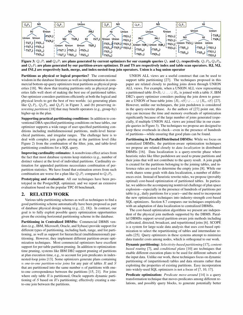
Figure 3: Q1P1 and Q2P1 are plans generated by current optimizers for our example queries Q1 and Q2 respectively. Q1P2, Q2P2,and Q2P3 are plans generated by our partition-aware optimizer. IS and TS are respectively index and table scan operators. HJ, MJ,and INLJ are respectively hash, merge, and index-nested-loop join operators. Union is a bag union operator

Partitions as physical or logical properties? The conventionalwisdom in the database literature as well as implementation in com-mercial bottom-up query optimizers treat partitions as physical prop-erties [18]. We show that treating partitions only as physical prop-erties falls well short of making the best use of partitioned tables.Our optimizer considers partitions efficiently at both the logical andphysical levels to get the best of two worlds: (a) generating planslike Q1P2, Q2P2, and Q2P3 in Figure 3, and (b) preserving in-teresting partitions [18] that may benefit operators (e.g., group-by)higher-up in the plan.Supporting practical partitioning conditions: In addition to con-ventional DBA-specified partitioning conditions on base tables, ouroptimizer supports a wide range of user-specified partitioning con-ditions including multidimensional partitions, multi-level hierar-chical partitions, and irregular ranges. The challenge here is todeal with complex join graphs arising at the partition level (likeFigure 2) from the combination of the filter, join, and table-levelpartitioning conditions for a SQL query.Improving cardinality estimates: A nonobvious effect arises fromthe fact that most database systems keep statistics (e.g., number ofdistinct values) at the level of individual partitions. Cardinality es-timation for appended partitions necessitates combination of per-partition statistics. We have found that estimation errors from suchcombination are worse for a plan like Q1P1 compared to Q1P2.Prototyping and evaluation: All our techniques have been pro-totyped in the PostgreSQL optimizer, and we report an extensiveevaluation based on the popular TPC-H benchmark.

2. RELATED WORKVarious table partitioning schemes as well as techniques to find a

good partitioning scheme automatically have been proposed as partof database physical design tuning (e.g., [2, 18]). In contrast, ourgoal is to fully exploit possible query optimization opportunitiesgiven the existing horizontal partitioning scheme in the database.Partitioning in Centralized DBMSs: Commercial DBMS ven-dors (e.g., IBM, Microsoft, Oracle, and Sybase) provide support fordifferent types of partitioning, including hash, range, and list parti-tioning, as well as support for hierarchical (multidimensional) par-titioning. However, they implement different partition-aware opti-mization techniques. Most commercial optimizers have excellentsupport for per-table partition pruning. In addition to optimization-time pruning, systems like IBM DB2 support pruning of partitionsat plan execution time, e.g., to account for join predicates in index-nested-loop joins [13]. Some optimizers generate plans containingn one-to-one partition-wise joins for any pair of tables R and Sthat are partitioned into the same number n of partitions with one-to-one correspondence between the partitions [15, 21]. For joinswhere only table R is partitioned, Oracle supports dynamic parti-tioning of S based on R’s partitioning; effectively creating a one-to-one join between the partitions.

UNION ALL views are a useful construct that can be used tosupport table partitioning [27]. The techniques proposed in thispaper are related closely to pushing joins down through UNIONALL views. For example, when a UNION ALL view representinga partitioned table R=R1 ∪ . . . ∪Rn is joined with a table S, IBMDB2’s query optimizer considers pushing the join down to gener-ate a UNION of base-table joins (R1./S) ∪ . . . ∪ (Rn./S) [27].However, unlike our techniques, the join pushdown is consideredin the query-rewrite phase. As the authors of [27] point out, thisstep can increase the time and memory overheads of optimizationsignificantly because of the large number of joins generated (espe-cially, if multiple UNION ALL views are joined like in our exam-ple queries in Figure 3). The techniques we propose are designed tokeep these overheads in check—even in the presence of hundredsof partitions—while ensuring that good plans can be found.Partitioning in Parallel/Distributed DBMSs: While we focus oncentralized DBMSs, the partition-aware optimization techniqueswe propose are related closely to data localization in distributedDBMSs [16]. Data localization is a query-rewrite phase whereheuristic rules like filter pushdown are used to prune partitions andtheir joins that will not contribute to the query result. A join graphis created for the partitions belonging to the joining tables, and in-ference rules are used to determine the empty joins [8]. While ourwork shares some goals with data localization, a number of differ-ences exist. Instead of heuristic rewrite rules, we propose (provablyoptimal) cost-based optimization of partitioned tables. In particu-lar, we address the accompanying nontrivial challenge of plan spaceexplosion—especially in the presence of hundreds of partitions pertable (e.g., daily partitions for a year)—and the need to incorporatethe new optimization techniques into industry-strength cost-basedSQL optimizers. Section 8.7 compares our techniques empiricallywith an adaptation of data localization to centralized DBMSs.

The cost-based optimization algorithms we present are indepen-dent of the physical join methods supported by the DBMS. Paral-lel DBMSs support several partition-aware join methods includingcollocated, directed, broadcast, and repartitioned joins [6]. SCOPEis a system for large-scale data analysis that uses cost-based opti-mization to select the repartitioning of tables and intermediate re-sults [25]. Query optimizers in these systems attempt to minimizedata transfer costs among nodes, which is orthogonal to our work.Dynamic partitioning: Selectivity-based partitioning [17], content-based routing [7], and conditional plans [10] are techniques thatenable different execution plans to be used for different subsets ofthe input data. Unlike our work, these techniques focus on dynamicpartitioning of (unpartitioned) tables and data streams rather thanexploiting the properties of existing partitions. Easy incorporationinto widely-used SQL optimizers is not a focus of [7, 10, 17].Predicate optimization: Predicate move-around [14] is a querytransformation technique that moves predicates among different re-lations, and possibly query blocks, to generate potentially better

plans. Magic sets [5] represent a complementary technique that cangenerate auxiliary tables to be used as early filters in a plan. Bothtechniques are applied in the rewrite phase of query optimization,thereby complementing our cost-based optimization techniques.

3. PROBLEM AND SOLUTION OVERVIEWOur goal is to generate an efficient plan for a SQL query that

contains joins of partitioned tables. In this paper, we focus on tablesthat are partitioned horizontally based on conditions specified onone or more partitioning attributes (columns). The condition thatdefines a partition of a table is an expression involving any numberof binary subexpressions of the form Attr Op Val, connected byAND or OR logical operators. Attr is an attribute in the table, Val isa constant, and Op is one of {=, 6=, <,≤, >,≥}.

Joins in a SQL query can be equi or nonequi joins. The joinedtables could have different numbers of partitions and could be par-titioned on multiple attributes (like in Figure 2). Furthermore, thepartitions between joined tables need not have one-on-one corre-spondence with each other. For example, a table may have onepartition per month while another table has one partition per day.

Our approach for partition-aware query optimization is based onextending bottom-up query optimizers. We will give an overviewof the well-known System R bottom-up query optimizer [19] onwhich a number of current optimizers are based, followed by anoverview of the extensions we make.

A bottom-up optimizer starts by optimizing the smallest expres-sions in the query, and then uses this information to progressivelyoptimize larger expressions until the optimal physical plan for thefull query is found. First, the best access path (e.g., table or indexscan) is found and retained for each table in the query. The bestjoin path is then found and retained for each pair of joining tablesR and S in the query. The join path consists of a physical join op-erator (e.g., hash or merge join) and the access paths found earlierfor the tables. Next, the best join path is found and retained for allthree-way joins in the query; and so on.

Bottom-up optimizers pay special attention to physical proper-ties (e.g., sort order) that affect the ability to generate the optimalplan for an expression e by combining optimal plans for subexpres-sions of e. For example, for R ./ S, the System R optimizer storesthe optimal join path for each interesting sort order [19] of R ./ Sthat can potentially reduce the plan cost of any larger expressionthat contains R ./ S (e.g., R ./ S ./ U ).Our extensions: Consider the join path selection in a bottom-upoptimizer for two partitioned tables R and S. R and S can bebase tables or the result of intermediate subexpressions. Let therespective partitions be R1-Rr and S1-Ss. For ease of exposition,we call R and S the parent tables in the join, and each Ri (Sj)a child table. By default, the optimizer will consider a join pathcorresponding to (R1∪· · ·∪Rr) ./ (S1∪· · ·∪Ss), i.e., a physicaljoin operator that takes the bag unions of the child tables as input.This approach leads to plans like Q1P1 and Q2P1 in Figure 3.

Partition-aware optimization must consider joins among the childtables in order to get efficient plans like Q1P2 in Figure 3; effec-tively, pushing the join below the union(s). Joins of the child tablesare called child joins. When the bottom-up optimizer considers thejoin of partitioned tables R and S, we extend its search space toinclude plans consisting of the union of child joins. This processworks in four phases: applicability testing, matching, clustering,and path creation.Applicability testing: We first check whether the specified joincondition between R and S match the partitioning conditions on Rand S appropriately. Intuitively, efficient child joins can be utilizedonly when the partitioning columns are part of the join attributes.

For example, the R.a = S.a join condition makes it possible toutilize the R2 ./ (S22 ∪ S23) child join in plan Q1P2 in Figure 3.Matching: This phase uses the partitioning conditions to determineefficiently which joins between individual child tables of R andS can potentially generate output records, and to prune the emptychild joins. For R ./ S in our running example query Q1, thisphase outputs {(R1, S12),(R1, S13),(R2, S22), (R2, S23)}.Clustering: Production deployments can contain tables with manytens to hundreds of partitions that lead to a large number of joinsbetween individual child tables.2 To reduce the join path creationoverhead, we carefully cluster the child tables; details are in Section5. ForR ./ S in our running example, the matching phase’s outputis clustered such that only the two child joins R1 ./ (S12 ∪ S13)and R2 ./ (S22 ∪ S23) are considered during path creation.Path Creation: This phase creates and costs join paths for all childjoins output by the clustering phase, as well as the path that repre-sents the union of the best child-join paths. This path will be chosenfor R ./ S if it costs lower than the one produced by the optimizerwithout our extensions.The next three sections give the details of these phases. Section 6will also discuss how our techniques can be incorporated into thebottom-up optimization process.

4. MATCHING PHASESuppose the bottom-up optimizer is in the process of selecting

the join path for parent tables R and S with respective child ta-bles R1-Rr and S1-Ss. The goal of the matching phase is to iden-tify all partition-wise join pairs (Ri, Sj) such that Ri ./ Sj canproduce output tuples as per the given partitioning and join condi-tions. Equivalently, this algorithm prunes out (from all possible joinpairs) partition-wise joins that cannot produce any results. An ob-vious matching algorithm would enumerate and check all the r× spossible child table pairs. In distributed query optimization, this al-gorithm is implemented by generating a join graph for the child ta-bles [8]. The real inefficiency from this quadratic algorithm comesfrom the fact that it gets invoked from scratch for each distinct joinof parent tables considered throughout the bottom-up optimizationprocess. Note that R and S can be base tables or the result of inter-mediate subexpressions.

We developed an efficient matching algorithm that builds, probes,and reuses Partition Index Trees (PITs). We will describe this newdata structure, and then explain how the matching algorithm uti-lizes it to generate the partition-wise join pairs efficiently. PITsapply to range and list partitioning conditions. Section 7 describeshow our techniques can be extended to handle hash partitioning.

4.1 Partition Index TreesThe core idea behind Partition Index Trees is to associate each

child table with one or more intervals generated from the table’spartitioning condition. An interval is specified as a Low to Highrange, which can be numeric (e.g., (0, 10]), date (e.g., [02-01-10,03-01-10)), or a single numeric or categorical value (e.g., [5, 5],[url,url]). A PIT indexes all intervals of all child tables for one ofthe partitioning columns of a parent table. The PIT then enablesefficient lookup of the intervals that overlap with a given probe in-terval from the other table. The use of PITs provides two mainadvantages:• For most practical partitioning and join conditions, building and

probing PITs has O(r log r) complexity (for r partitions in atable). The memory needs are θ(r).

2We are aware of such deployments in a leading social networkingcompany and for a commercial parallel DBMS.

Figure 4: A partition index tree containing intervals for allchild tables (partitions) of T from Figure 2

• Most PITs are built once and then reused many times over thecourse of the bottom-up optimization process (see Section 4.4).

Implementation: PIT, at a basic level, is an augmented red-blacktree [9]. The tree is ordered by the Low values of the intervals,and an extra annotation is added to every node recording the max-imum High value (denoted Max) across both its subtrees. Figure4 shows the PIT created on attribute T.a based on the partitioningconditions of all child tables of T (see Figure 2). The Low and Maxvalues on each node are used during probing to efficiently guidethe search for finding the overlapping intervals. When the interval[20, 40) is used to probe the PIT, five intervals are checked (high-lighted in Figure 4) and the two overlapping intervals [20, 30) and[30, 40) are returned.

A number of nontrivial enhancements to PITs were needed tosupport complex partitioning conditions that can arise in practice.First, PITs need support for multiple types of intervals: open, closed,partially closed, one sided, and single values (e.g., (1, 5), [1, 5],[1, 5), (−∞, 5], and [5, 5]). In addition, supporting nonequi joinsrequired support from PITs to efficiently find all intervals in the treethat are to the left or to the right of the probe interval.

Both partitioning and join conditions can be complex combina-tions of AND and OR subexpressions, as well as involve any oper-ator in {=, 6=, <,≤, >,≥}. Our implementation handles all thesecases by restricting PITs to unidimensional indexes and handlingcomplex expressions appropriately in the matching algorithm.

4.2 Matching AlgorithmFigure 5 provides all the steps for the matching algorithm. The

input consists of the two tables to be joined and the join condition.We will describe the algorithm using query Q1 in our running ex-ample from Section 1. The join condition for S ./ T in Q1 is asimple equality expression: S.a = T.a. Later, we will discuss howthe algorithm handles more complex conditions involving logicalAND and OR operators, as well as nonequi join conditions. Sincethe matching phase is executed only if the Applicability Test passes(see Section 3), the attributes S.a and T.a must appear in the parti-tioning conditions for the partitions of S and T respectively.

The table with the smallest number of (unpruned) partitions isidentified as the build relation and the other as the probe relation.In our example, T (with 3 partitions) will be the build relation andS (with 4 partitions) will be the probe one. Since partition pruningis performed before any joins are considered, only the unprunedchild tables are used for building and probing the PIT. Then, thematching algorithm works as follows:• Build phase: For each child table Ti of T , generate the interval

for Ti’s partitioning condition (explained in Section 4.3). Builda PIT that indexes all intervals from the child tables of T .• Probe phase: For each child table Sj of S, generate the inter-

val int for Sj’s partitioning condition. Probe the PIT on T.a tofind intervals overlapping with int. Only T ’s child tables corre-

Algorithm for performing the matching phaseInput: Relation R, Relation S, Join ConditionOutput: All partition-wise join pairs (Ri,Sj ) that can produce join resultsFor each (binary join expression in Join Condition) {

Convert all partitioning conditions to intervals;Build PIT with intervals from partitions of R;Probe the PIT with intervals from partitions of S;Adjust matching result based on logical AND or OR semantics of the

Join Condition;}

Figure 5: Matching algorithm

sponding to these overlapping intervals can have tuples joiningwith Sj ; output the identified join pairs.

For S ./ T in our running example query, the PIT on T.a willcontain the intervals [0, 10), [10, 20) and [20, 30), which are asso-ciated with partitions T1, T2, and T3 respectively (Figure 2). Whenthis PIT is probed with the interval [20, 40) for child table S22,the result will be the interval [20, 30); indicating that only T3 willjoin with S22. Overall, this phase outputs {(S12, T1), (S12, T2),(S13, T1), (S13, T2), (S22, T3), (S23, T3)}; the remaining possi-ble child joins are pruned.

4.3 Support for Complex ConditionsBefore building and probing the PIT, we need to convert each

partitioning condition into one or more intervals. A condition couldbe any expression involving logical ANDs, ORs, and binary expres-sions. Subexpressions that are ANDed together are used to build asingle interval, whereas subexpressions that are ORed together willproduce multiple intervals. For example, suppose the partitioningcondition is (R.a ≥ 0 AND R.a < 20). This condition will createthe interval [0, 20). The condition (R.a > 0 AND R.b > 5) willcreate the interval (0,∞), since only R.a appears in the join con-ditions of query Q1. The condition (R.a < 0 OR R.a > 10) willcreate the intervals (−∞, 0) and (10,∞). If the particular condi-tion does not involveR.a, then the interval created is (−∞,∞), asany value for R.a is possible.

Our approach can also support nonequi joins, for exampleR.a <S.a. The PIT was adjusted in order to efficiently find all inter-vals in the PIT that are to the left or to the right of the providedinterval. Suppose A = (A1, A2) is an interval in the PIT andB = (B1, B2) is the probing interval. The interval A is markedas an overlapping interval if ∃α∈A,β∈B such that α < β. Notethat this check is equivalent to finding all intervals in the PIT thatoverlap with the interval (−∞, B2).

Finally, we support complex join expressions involving logicalANDs and ORs. Suppose the join condition is (R.a = S.a ANDR.b = S.b). In this case, two PITs will be built; one for R.a andone forR.b. After probing the two PITs, we will get two sets of joinpairs. We then adjust the pairs based on whether the join conditionsare ANDed or ORed together. In the example above, suppose thatR1 can join with S1 based on R.a, and that R1 can join with bothS1 and S2 based on R.b. Since the two binary join expressionsare ANDed together, we induce that R1 can join only with S1.However, if the join condition were (R.a = S.a OR R.b = S.b),then we would induce that R1 can join with both S1 and S2.

4.4 Complexity AnalysisSuppose N and M are the number of partitions for the build

and probe relations respectively. Also suppose each partition con-dition is translated into a small, fixed number of intervals (whichis usually the case). In fact, a simple range partitioning conditionwill generate exactly one interval. Then, building a PIT requiresO(N × logN) time. Probing a PIT with a single interval takes

Figure 6: Clustering algorithm applied to example query Q1

O(min(N, k × logN)) time, where k is the number of matchingintervals. Hence, the overall time to identify all possible child joinpairs is O(M ×min(N, k × logN)).

The space overhead introduced by a PIT is θ(N) since it is abinary tree. However, a PIT can be reused multiple times during theoptimization process. Consider the join condition (R.a=S.a ANDS.a=T.a) for tables R, S, and T in Q1. A PIT built for S.a can be(re)used for performing the matching algorithm when consideringthe joins R ./ S, S ./ T , (R ./ S) ./ T , and (S ./ T ) ./ R.

5. CLUSTERING PHASEThe number of join pairs output by the matching phase can be

large, e.g., when each child table of R joins with multiple childtables of S. In such settings, it becomes important to reduce thenumber of join pairs that need to be considered during join path cre-ation to avoid both optimization and execution inefficiencies. Joinpath creation introduces optimization-time overheads for enumer-ating join operators, accessing catalogs, and calculating cardinalityestimates. During execution, if multiple child-join paths referencethe same child table Ri, then Ri will be accessed multiple times; asituation we want to avoid.

The approach we use to reduce the number of join pairs is tocluster together multiple child tables of the same parent table. Fig-ure 6 considers S ./ T for query Q1 from Section 1. The sixpartition-wise join pairs output by the matching phase are shownon the left. Notice that the join pairs (S22, T3) and (S23, T3) indi-cate that both S22 and S23 can join with T3 to potentially generateoutput records. If S22 is clustered with S23, then the single (clus-tered) join (S22∪S23) ./ T3 will be considered in the path creationphase instead of the two joins S22 ./ T3 and S23 ./ T3. Further-more, because of the clustering, the child table T3 will have onlyone access path (say, a table or index scan) in Q1’s plan.

Definition 1. Clustering metric: For an R ./ S join, two (un-pruned) child tables Sj and Sk of S will be clustered together iffthere exists a (unpruned) child tableRi ofR such that the matchingphase outputs the join pairs (Ri, Sj) and (Ri, Sk). 2

If Sj and Sk are clustered together when no such Ri exists, thenthe union of Sj and Sk will lead to unneeded joins with child tablesof R; hurting plan performance during execution. In our runningexample in Figure 6, suppose we cluster S22 with S13. Then, S22

will have to be considered unnecessarily in joins with T1 and T2.On the other hand, failing to cluster Sj and Sk together when

the matching phase outputs the join pairs (Ri, Sj) and (Ri, Sk)would result in considering join paths separately for Ri ./ Sj andRi ./ Sk. The result is higher optimization overhead as well asaccess of Ri in at least two separate paths during execution. Inour example, if we consider separate join paths for S22 ./ T3 andS23 ./ T3, then partition T3 will be accessed twice.Clustering algorithm: Figure 7 shows the clustering algorithmthat takes as input the join pairs output by the matching phase. Thealgorithm first constructs the join partition graph from the input

Algorithm for clustering the output of the matching phaseInput: Partition join pairs (output of matching phase)Output: Clustered join pairs (which will be input to path creation phase)Build a bipartite join graph from the input partition join pairs where:

Child tables are the vertices, andPartition join pairs are the edges;

Use Breadth-First-Search to identify connected components in the graph;Output a clustered join pair for each connected component;

Figure 7: Clustering algorithm

join pairs. Each child table is a vertex in this bipartite graph, andeach join pair forms an edge between the corresponding vertices.Figure 6 shows the join partition graph for our example. Breadth-First-Search is used to identify all the connected components in thejoin partition graph. Each connected component will give a (pos-sibly clustered) join pair. Following our example in Figure 6, S12

will be clustered with S13, S22 with S23, and T1 with T2, formingthe output of the clustering phase consisting of the two (clustered)join pairs ({S12, S13}, {T1, T2}) and ({S22, S23}, {T3}).

6. PATH CREATION AND SELECTIONWe will now consider how to create and cost join paths for all

the (clustered) child joins output by the clustering phase, as wellas the union of the best child-join paths. Join path creation has tobe coupled tightly with the physical join operators supported bythe database system. As discussed in Section 1.2, we will leveragethe functionality of a bottom-up query optimizer [19] to create joinpaths for the database system. The main challenge is how to extendthe enumeration and path retention aspects of a bottom-up queryoptimizer in order to find the optimal plan in the new extended planspace efficiently.Definition 2. Optimal plan in the extended plan space: In ad-dition to the default plan space considered by the bottom-up opti-mizer for an n-way (n≥2) join of parent tables, the extended planspace includes the plans containing any possible join order and joinpath for joins of the child tables such that each child table (parti-tion) is accessed at most once. The optimal plan is the plan withleast estimated cost in the extended plan space. 2

We will discuss three different approaches on how to extend thebottom-up optimizer to find the optimal plan in the extended planspace. Query Q1 from Section 1 is used as an example throughout.

Note that Q1 joins the three parent tables R, S, and T . For Q1,a bottom-up optimizer will consider the three 2-way joins R ./ S,R ./ T , S ./ T , and the single 3-way join R ./ S ./ T . Foreach join considered, the optimizer will find and retain the best joinpath for each interesting order and the best “unordered” path. Sortorders onR.a, S.a, and T.a are the candidate interesting orders forQ1. When the optimizer is considering an n-way join, it only usesthe best join paths retained for smaller joins.

6.1 Extended EnumerationThe first approach is to extend the existing path creation process

that occurs during the enumeration of each possible join. The ex-tended enumeration includes the path representing the union of thebest child-join paths for the join. For instance, as part of the enu-meration process for query Q1, the optimizer will create and costjoin paths for S ./ T . The conventional join paths include joiningthe union of S’s partitions with the union of T ’s partitions usingall applicable join operators (like hash join or merge join), leadingto plans like Q1P1 in Figure 3. At this point, extended enumera-tion will also create join paths for (S12 ∪ S13) ./ (T1 ∪ T2) and(S22 ∪ S23) ./ T3, find the corresponding best paths, and createthe union of the best child-join paths. We will use the notation Pu

in this section to denote the union of the best child-join paths.

As usual, the bottom-up optimizer will retain the best join pathfor each interesting order (a in this case) as well as the best (pos-sibly unordered) overall path. If Pu is the best for one of thesecategories, then it will be retained. The paths retained will be theonly paths considered later when the enumeration process moveson to larger joins. For example, when creating join paths for (S ./T ) ./ R, only the join paths retained for S ./ T will be used (inaddition to the access paths retained for R).Property 1. Adding extended enumeration to a bottom-up opti-mizer will not always find the optimal plan in the extended planspace. 2

We will prove Property 1 using our running example. Suppose planPu for S ./ T is not retained because it is not a best path for anyorder. Without Pu for S ./ T , when the optimizer goes on toconsider (S ./ T ) ./ R, it will not be able to consider any 3-waychild join. Thus, plans similar toQ1P2 from Figure 3 will never beconsidered; thereby losing the opportunity to find the optimal planin the extended plan space.

6.2 Treating Partitions as a Physical PropertyThe next approach considers partitioning as a physical property

of tables and the output of partition-wise joins. The parallel editionof DB2 follows this approach. The concept of interesting partitions(similar to interesting orders) can be used to incorporate partition-ing as a physical property in the bottom-up optimizer. Interest-ing partitions are partitions on attributes referenced in equality joinconditions and on grouping attributes [18]. In our example queryQ1, partitions on attributes R.a, S.a, and T.a are interesting.

Paths with interesting partitions can make later joins and group-ing operations less expensive when these operations can take ad-vantage of the partitioning. For example, partitioning on S.a forS ./ T could lead to the creation of three-way child joins forR ./ S ./ T . Hence, the optimizer will retain the best path for eachinteresting partition, in addition to each interesting order. Overall,if there are n interesting orders and m interesting partitions, thenthe optimizer can retain up to n×m paths, one for each combina-tion of interesting orders and interesting partitions.Property 2. Treating partitioning as a physical property in a bottom-up optimizer will not always find the optimal plan in the extendedplan space. 2

Once again we will prove the above property using the examplequery Q1. When the optimizer enumerates paths for S ./ T , itwill consider Pu (the union of the best child-join paths). Unlikewhat happened in extended enumeration, Pu will now be retainedsince Pu has an interesting partition on S.a. Suppose the first andsecond child joins of Pu have the respective join paths (S12 ∪S13)HJ (T1 ∪ T2) and (S22 ∪ S23) HJ T3. (HJ and MJ denote hashand merge join operators respectively.) Also, the best join path forS ./ T with an interesting order on S.a is the union of the child-join paths (S12 ∪ S13) MJ (T1 ∪ T2) and (S22 ∪ S23) MJ T3.

However, it can still be the case that the optimal plan for Q1 isplan Q1P2 shown in Figure 3. Note that Q1P2 contains (S12 ∪S13) MJ (T1 ∪ T2): the interesting order on S.a in this child joinled to a better overall plan. However, the interesting order on S.awas not useful in the case of the second child join of S ./ T , so(S22 ∪S23) MJ T3 is not used in Q1P2. Simply adding interestingpartitions alongside interesting orders to a bottom-up optimizer willnot enable it to find the optimal plan Q1P2.

The optimizer was not able to generate plan Q1P2 in the aboveexample because it did not consider interesting orders indepen-dently for each child join. Instead, the optimizer considered in-teresting orders and interesting partitions at the level of the parenttables (R, S, T ) and joins of parent tables (R ./ S, R ./ T ,

Figure 8: Logical relations (with child relations) enumeratedfor query Q1 by our partition-aware bottom-up optimizer

S ./ T , R ./ S ./ T ) only. An apparent solution would be forthe optimizer to create union plans for all possible combinations ofchild-join paths with interesting orders. However, the number ofsuch plans is exponential in the number of child joins per parentjoin, rendering this approach impractical.

6.3 Treating Partitions as a Logical PropertyOur approach eliminates the aforementioned problems by treat-

ing partitioning as a property of the logical relations (tables orjoins) that are enumerated during the bottom-up optimization pro-cess. A logical relation refers to the output produced by either ac-cessing a table or joining multiple tables together. For example, thelogical relation (join) RST represents the output produced whenjoining the tables R, S, and T , irrespective of the join order or thejoin operators used in the physical execution plan. Figure 8 showsall logical relations created during the enumeration process for ourexample query Q1.

As illustrated in Figure 8, each logical relation maintains a listof logical child relations. A logical child table is created for eachunpruned partition during partition pruning, whereas logical childjoins are created based on the output of the clustering phase. Forour example query Q1, the child-join pairs ({S12, S13}, {T1, T2})and ({S22, S23}, {T3}) output by the clustering phase are used tocreate the respective logical child joins S12S13T1T2 and S22S23T3.The logical child relations also maintain the partitioning conditions,which are propagated up when the child joins are created.

For each logical n-way join relation Jn = Jn−1 ./ J1, the logi-cal child relations and partitioning conditions of Jn−1 and J1 formthe input to Jn’s matching phase (Section 4). The output of thematching phase forms the input to Jn’s clustering phase (Section5) which, in turn, outputs Jn’s logical child joins. Note that boththe matching and clustering phases work at the logical level, inde-pendent of physical plans (paths).

The logical relations are the entities for which the best pathsfound so far during the enumeration process are retained. The log-ical child joins behave in the same way as their parent joins, retain-ing the best paths for each interesting order and the best unorderedpath. Hence, the number of paths retained is linear in the numberof child joins per parent join (instead of exponential as in the casewhen partitions are treated as physical properties). The optimizerconsiders all child-join paths with interesting orders during pathcreation for higher child joins, while ensuring the property:

Property 3. Paths with interesting orders for a single child join canbe used later up the lattice, independent from all other child joinsof the same parent relation. 2

Suppose, the optimizer is considering joining ST with R to createpaths for RST . The output of the clustering phase will producethe two child-join pairs (S12S13T1T2, R1) and (S22S23T3, R2).Join paths for these two child joins will be created and costed in-dependently from each other, using any paths with interesting or-ders and join operators that are available. The best join paths for((S12 ∪ S13) ./ (T1 ∪ T2)) ./ R1 and ((S22 ∪ S23) ./ T3) ./R2) will be retained in the logical relations R1S12S13T1T2 andR2S22S23T3 respectively (see Figure 8).

For each parent relation, the path representing the union of thebest child-join paths is created only at the end of each enumera-tion level3 and it is retained only if it is the best path. Hence, theoptimizer will consider all join orders for each child join beforecreating the union, leading to the following property:Property 4. The optimizer will consider plans where different childjoins of the same parent relation can have different join ordersand/or join operators. 2

We have already seen how the optimizer created join paths ((S12 ∪S13) ./ (T1 ∪ T2)) ./ R1 and ((S22 ∪ S23) ./ T3) ./ R2 whenjoining ST with R. Later, the optimizer will consider joining RSwith T , creating join paths for (R1 ./ (S12 ∪ S13)) ./ (T1 ∪ T2)and (R2 ./ (S22 ∪ S23)) ./ T3. It is possible that the best joinpath for ((S12 ∪ S13) ./ (T1 ∪ T2)) ./ R1 is better than thatfor (R1 ./ (S12 ∪ S13)) ./ (T1 ∪ T2), while the opposite occursbetween ((S22∪S23) ./ T3) ./ R2 and (R2 ./ (S22∪S23)) ./ T3;which leads to the plan Q1P2 in Figure 3.Property 5. Optimality guarantee: By treating partitioning as alogical property, our bottom-up optimizer will find the optimal planin the extended plan space. 2

This property is a direct consequence of Properties 3 and 4. Wehave extended the plan space to include plans containing unionsof child joins. Each child join is enumerated during the traditionalbottom-up optimization process in the same way as its parent; thepaths are built bottom-up, interesting orders are taken into consid-eration, and the best paths are retained. Since each child join isoptimized independently, the topmost union of the best child-joinpaths is the optimal union of the child joins. Finally, recall that theunion of the best child-join paths is created at the end of each enu-meration level and retained only if it is the best plan for its parentjoin. Therefore, the full extended plan space is considered and theoptimizer will be able to find the optimal plan (given the currentdatabase configuration, cost model, and physical design).

Traditionally, grouping (and aggregation) operators are added ontop of the physical join trees produced by the bottom-up enumera-tion process [19]. In this case, interesting partitions are useful forpushing the grouping below the union of the child joins, in an at-tempt to create less expensive execution paths. With our approach,paths with interesting partitions on the grouping attributes can beconstructed at the top node of the enumeration lattice, and usedlater on while considering the grouping operator.

Treating partitions as a property of the logical relations allowsfor a clean separation between the enumeration process of the log-ical relations and the construction of the physical plans. Hence,our algorithms are applicable to any database system that uses abottom-up optimizer. Moreover, they can be adapted for non-databasedata processing systems like SCOPE and Hive that offer support fortable partitioning and joins.3Enumeration level n refers to the logical relations representing allpossible n-way joins.

Name FeaturesBasic Per-table partition pruning only (like MySQL and Post-

greSQL). Our evaluation uses the PostgreSQL 8.3.7 op-timizer as the Basic optimizer

Intermediate Per-table partition pruning and one-to-one partition-wisejoins (like Oracle and SQLServer). The Intermediate op-timizer is implemented as a variant of the Advanced op-timizer that checks for and creates one-to-one partition-wise join pairs in place of the regular matching and clus-tering phases

Advanced Per-table partition pruning and all the join optimizationsfor partitioned tables as described in the paper

Table 2: Optimizer categories considered in the evaluation

7. EXTENDING OUR TECHNIQUES TOPARALLEL DATABASE SYSTEMS

While this paper focuses on centralized DBMSs, our work is alsouseful in parallel DBMSs like Aster nCluster [3], Teradata [22], andHadoopDB [1] which try to partition tables such that most queriesin the workload need intra-node processing only. A common dataplacement strategy in parallel DBMSs is to use hash partitioning todistribute tuples in a table among the nodes N1, . . . , Nk, and thenuse range/list partitioning of the tuples within each node. Our tech-niques extend to this setting: if two joining tablesR and S have thesame hash partitioning function and the same number of partitions,then a partition-wise joinRi ./ Si is created for each nodeNi. If asecondary range/list partitioning has been used to further partitionRi and Si at an individual node, then our techniques can be applieddirectly to produce child joins for Ri ./ Si.

Another data placement strategy popular in data warehouses isto replicate the dimension tables on all nodes, while the fact tableis partitioned across the nodes. The fact-table partition as well asthe dimension tables may be further partitioned on each node, soour techniques can be used to create child joins at each node. Insuch settings, multi-dimensional partitioning of the fact table canimprove query performance significantly as we show in Section 8.

8. EXPERIMENTAL EVALUATIONThe purpose of this section is to evaluate the effectiveness and ef-

ficiency of our optimization techniques across a wide range of fac-tors that affect table partitioning. We have prototyped all our tech-niques in the PostgreSQL 8.3.7 optimizer. All experiments wererun on Amazon EC2 nodes of m1.large type. Each node has 7.5GBRAM, dual-core 2GHz CPU, and 850GB of storage. We used theTPC-H benchmark with scale factors ranging from 10 to 40, with30 being the default scale. Following directions from the TPC-HStandard Specifications [23], we partitioned tables only on primarykey, foreign key, and/or date columns. We present experimentalresults for a representative set of 10 out of the 22 TPC-H queries,ranging from 2-way up to the maximum possible 8-way joins. Allresults presented are averaged over three query executions.

8.1 Experimental SetupThe most important factor affecting query performance over par-

titioned tables is the partitioning scheme that determines which ta-bles are partitioned and on which attribute. We identified two casesthat arise in practice:1. The DBA has full control in selecting and deploying the parti-

tioning scheme to maximize query-processing efficiency.2. The partitioning scheme is forced either partially or fully by

practical reasons beyond query-processing efficiency.For evaluation purposes, we categorized query optimizers into threecategories—Basic, Intermediate, and Advanced—based on how theyexploit partitioning information to perform optimization. Details

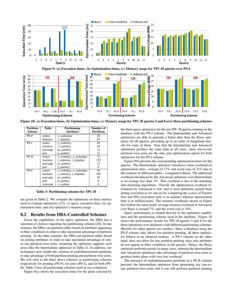
Figure 9: (a) Execution times, (b) Optimization times, (c) Memory usage for TPC-H queries over PS-J

Figure 10: (a) Execution times, (b) Optimization times, (c) Memory usage for TPC-H queries 5 and 8 over three partitioning schemes

Partition Table Partitioning Number ofScheme Attributes Partitions

PS-P orders o_orderdate 28lineitem l_shipdate 85

PS-J orders o_orderkey 48lineitem l_orderkey 48partsupp ps_partkey 12part p_partkey 12

PS-B orders o_orderkey, o_orderdate 72lineitem l_orderkey, l_shipdate 120partsupp ps_partkey 12part p_partkey 6

PS-C orders o_orderkey, o_orderdate 36lineitem l_orderkey, l_shipdate 168partsupp ps_partkey 30part p_partkey 6customer c_custkey 6

Table 3: Partitioning schemes for TPC-H

are given in Table 2. We compare the optimizers on three metricsused to evaluate optimizers [12]: (i) query execution time, (ii) op-timization time, and (iii) optimizer’s memory usage.

8.2 Results from DBA-Controlled SchemesGiven the capabilities of the query optimizer, the DBA has a

spectrum of choices regarding the partitioning scheme [26]. In oneextreme, the DBA can partition tables based on attributes appearingin filter conditions in order to take maximum advantage of partitionpruning. At the other extreme, the DBA can partition tables basedon joining attributes in order to take maximum advantage of one-to-one partition-wise joins; assuming the optimizer supports suchjoins (like the Intermediate optimizer in Table 2). In addition, ourtechniques now enable the creation of multidimensional partitionsto take advantage of both partition pruning and partition-wise joins.We will refer to the three above schemes as partitioning schemesrespectively for pruning (PS-P), for joins (PS-J), and for both (PS-B). Table 3 lists all partitioning schemes used in our evaluation.

Figure 9(a) shows the execution times for the plans selected by

the three query optimizers for the ten TPC-H queries running on thedatabase with the PS-J scheme. The Intermediate and Advancedoptimizers are able to generate a better plan than the Basic opti-mizer for all queries, providing up to an order of magnitude ben-efit for some of them. Note that the Intermediate and Advancedoptimizers produce the same plan in all cases, since one-to-onepartition-wise joins are the only join optimization option for bothoptimizers for the PS-J scheme.

Figure 9(b) presents the corresponding optimization times for thequeries. The Intermediate optimizer introduces some overhead onoptimization time—average of 17% and worst case of 21% due tothe creation of child-join paths—compared to Basic. The additionaloverhead introduced by the Advanced optimizer over Intermediateis on average less than 3%. This overhead is due to the matchingand clustering algorithms. Overall, the optimization overhead in-troduced by Advanced is low, and is most definitely gained backduring execution as we can see by comparing the y-axes of Figures9(a) and 9(b) (execution time is in minutes whereas optimizationtime is in milliseconds). The memory overheads shown in Figure9(c) follow the same trend: average memory overhead of Advancedover Basic is around 7%, and the worst case is 10%.

Query performance is related directly to the optimizer capabil-ities and the partitioning scheme used in the database. Figure 10shows the performance results for TPC-H queries 5 and 8 for thethree optimizers over databases with different partitioning schemes.(Results for other queries are similar.) Since a database using thePS-P scheme only allows for partition pruning, all three optimiz-ers behave in an identical manner. A PS-J scheme on the otherhand, does not allow for any partition pruning since join attributesdo not appear in filter conditions in the queries. Hence, the Basicoptimizer performs poorly in many cases, whereas the Intermediateand Advanced optimizers take advantage of partition-wise joins toproduce better plans with very low overhead.

The presence of multidimensional partitions in a PS-B schemeprevents the Intermediate optimizer from generating any one-to-one partition-wise joins, but it can still perform partition pruning

Figure 11: (a) Execution times, (b) Optimization times, (c) Memory usage for TPC-H queries over PS-C with partition size 128MB

Figure 12: (a) Execution times, (b) Optimization times, (c) Memory usage as we vary the partition size for TPC-H queries 5 and 8

like the Basic optimizer. The Advanced optimizer utilizes bothpartition pruning and partition-wise joins to find better-performingplans. Consider the problem of picking the best partitioning schemefor a given query workload. The best query performance can be ob-tained either from (a) partition pruning (PS-P is best for query 8 inFigure 10), or (b) from partition-aware join processing (PS-J is bestfor query 5 in Figure 10), or (c) from a combination of both due tosome workload or data properties. In all cases, the Advanced opti-mizer enables finding the plan with the best possible performance.

8.3 Results from Constrained SchemesAs discussed in Section 1, external constraints or objectives may

limit the partitioning scheme that can be used. For instance, dataarrival rates may require the creation of daily or weekly partitions;file-system properties may impose a maximum partition size to en-sure that each partition is laid out contiguously; or optimizer limi-tations may impose a maximum number of partitions per table.

For a TPC-H scale factor of 30, biweekly partitions of the fact ta-ble lead to a 128MB partition size. We will impose a maximum par-tition size of 128MB to create the partitioning scheme PS-C used inthis section (see Table 3). Figure 11 shows the results for the TPC-H queries executed over a database with the PS-C scheme. Theconstraint imposed on the partitioning scheme does not allow forany one-to-one partition-wise joins. Hence, the Intermediate opti-mizer produces the same plans as Basic, and is excluded from thefigures for clarity. Once again, the Advanced optimizer was able togenerate a better plan than the Basic optimizer for all queries, pro-viding over 2x speedup for 50% of them. The average optimizationtime and memory overheads were just 7.9% and 3.6% respectively.

8.4 Effect of Size and Number of PartitionsIn this section, we evaluate the performance of the optimizers

as we vary the size (and thus the number) of partitions created foreach table, using the PS-C scheme. As we vary the partition sizefrom 64MB to 256MB, the number of partitions for the fact tablevary from 336 to 84. Figure 12(b) shows the optimization timestaken by the two optimizers for TPC-H queries 5 and 8. As the

Figure 13: Execution times as we vary the total data size

partition size increases (and the number of partitions decreases),the optimization time decreases for both optimizers. We observethat (i) the optimization times for the Advanced optimizer scalein a similar way as for the Basic optimizer, and (ii) the overheadintroduced by the creation of the partition-wise joins remains small(around 12%) in all cases.

The overhead added by our approach remains low due to tworeasons. First, Clustering bounds the number of child joins forR ./ S to min(number of partitions in R,S); so we cause only alinear increase in paths enumerated per join. Second, optimizershave other overheads like parsing, rewrites, scan path enumeration,catalog and statistics access, and cardinality estimation. Let us con-sider Query 5 from Figure 12(b). Query 5 joins 5 tables, includingorders and lineitem with 72 and 336 partitions respectively. In thiscase, Basic enumerated 2317 scan and join paths in total, whileAdvanced enumerated 2716 paths. The extra 17% paths are forthe 72 partition-wise joins created by Advanced. The trends aresimilar for the memory consumption of the optimizers as seen inFigure 12(c).

Decreasing the partition size for the same total data size has apositive effect on plan execution times as seen in Figure 12: smaller

Figure 14: (a) Execution times, (b) Optimization times, (c) Memory usage as we vary the number of tables joined on the sameattribute for a modified TPC-H schema and queries 2 and 5

Figure 15: (a) Execution times, (b) Optimization times, (c) Memory usage for enabling and disabling clustering

partition sizes force finer-grained partition ranges, leading to betterpartition pruning and join execution. Looking into execution timesat the subplan level, we observed that PostgreSQL was more effec-tive in our experimental settings when it accessed partitions in the64MB range. It is worth noting that current partitioning schemerecommenders [2, 18, 26] do not consider partition size tuning.

8.5 Effect of Data SizeWe used the PS-C scheme with a partition size of 128 MB to

study the effects of the overall data size on query performance. Fig-ure 13 shows the query execution times as the amount of data storedin the database increases. For many queries, the plans selected bythe Basic optimizer lead to a quadratic or exponential increase inexecution time as data size increases linearly. We observed thatjoins for large data sizes cause the Basic optimizer to frequently re-sort to index nested loop joins (the system has 7.5GB RAM only).

On the other hand, the Advanced optimizer is able to generatesmaller partition-wise joins that use more efficient join methods(like hash and merge joins); leading to the desired linear increasein execution time as data size increases linearly. For the querieswhere the Basic optimizer is also able to achieve a linear trend, theslope is much higher compared to the Advanced optimizer. Fig-ure 13 shows that the benefits from our approach become moreimportant for larger databases. Note that optimization times andmemory consumption are independent of the data size.

8.6 Stress Testing on a Synthetic BenchmarkThere exist practical scenarios where multiple tables may share a

common joining key. In Web analytics, for example, customer datamay reside in multiple tables—storing information such as pageclicks, favorites, preferences, etc.—that have to be joined on thecustomer key. However, in traditional star and snowflake schemas,the fact tables join with the dimension tables on different attributes;so it is hard to create n-way child joins for n ≥ 3. No TPC-H queryplan, regardless of the partitioning schema, contains n-way childjoins for n ≥ 4. To evaluate our approach in non-star schemas,as well as to stress-test our approach, we came up with a synthetic

partitioning schema where the tables part and orders from TPC-Hare partitioned vertically into four tables each. Once again, we usethe PS-C scheme with a partition size of 128 MB.

We modified TPC-H queries 2 and 5 to join all the vertical tablesfor part and orders respectively. Figure 14(a) shows the executiontimes for the two queries with increasing number of joining tables.We observe how the Advanced optimizer was again able to generateplans that are up to an order of magnitude better compared to theplans selected by the Basic optimizer. It is interesting to note that asthe number of joining tables in the query increases, the executiontimes for the plans from the Advanced optimizer increase barely(due to efficient use of child joins); unlike the Basic optimizer’splans whose execution times increase drastically.

Figures 14(b) and 14(c) show the optimization times and mem-ory consumption, respectively, as the number of “same-key-joining”tables in the query increases. Both metrics increase non-linearlyfor both optimizers; but the increase is more profound for the Ad-vanced optimizer. The increasing optimization overhead comesfrom the non-linear complexity of the path selection process usedby the regular PostgreSQL query optimizer (which we believe canbe fixed through engineering effort unrelated to our work). Withoptimization times still in milliseconds, the additional overhead iscertainly justified by the drastic reduction in execution times.

8.7 Effect of the Clustering AlgorithmClustering (Section 5) is an essential phase in our overall partition-

aware optimization approach that is missing from the data localiza-tion approach discussed in Section 2. When matching is appliedwithout clustering, our optimizer implements a rough equivalentof the four-phase approach to distributed query optimization [16].Figures 15(b) and 15(c) compare the optimization time and mem-ory consumption of the optimizer when clustering is enabled anddisabled in a database with the PS-C scheme. Disabling clusteringcauses high overhead—as seen in both figures—since the optimizermust now generate join paths for each child join produced by thematching phase. This issue shows why clustering is essential for

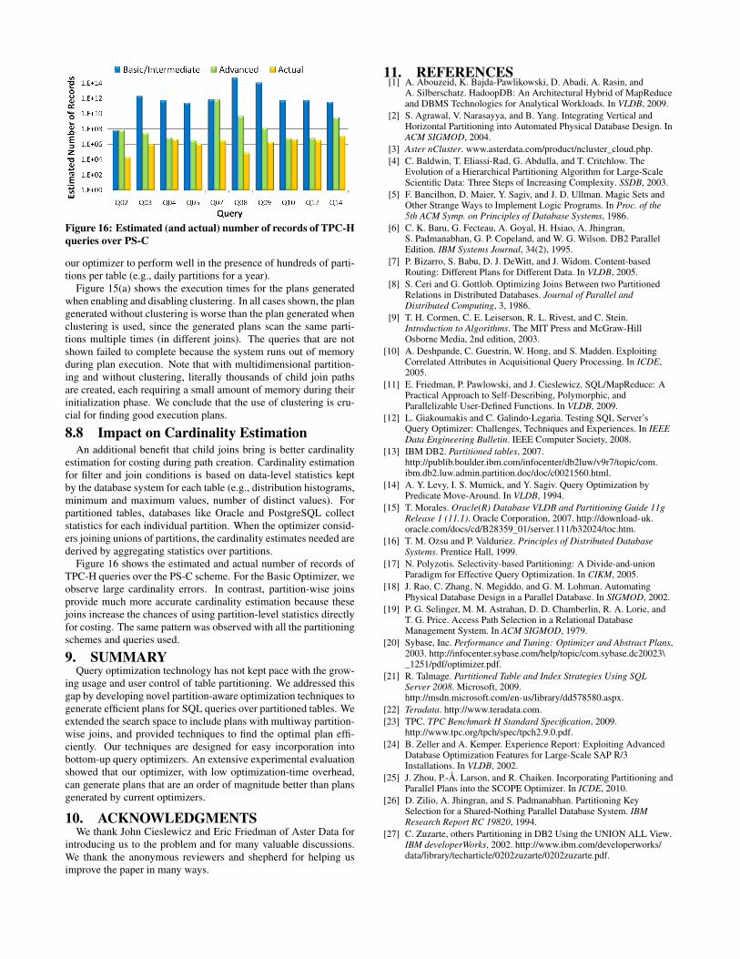
Figure 16: Estimated (and actual) number of records of TPC-Hqueries over PS-C

our optimizer to perform well in the presence of hundreds of parti-tions per table (e.g., daily partitions for a year).

Figure 15(a) shows the execution times for the plans generatedwhen enabling and disabling clustering. In all cases shown, the plangenerated without clustering is worse than the plan generated whenclustering is used, since the generated plans scan the same parti-tions multiple times (in different joins). The queries that are notshown failed to complete because the system runs out of memoryduring plan execution. Note that with multidimensional partition-ing and without clustering, literally thousands of child join pathsare created, each requiring a small amount of memory during theirinitialization phase. We conclude that the use of clustering is cru-cial for finding good execution plans.

8.8 Impact on Cardinality EstimationAn additional benefit that child joins bring is better cardinality

estimation for costing during path creation. Cardinality estimationfor filter and join conditions is based on data-level statistics keptby the database system for each table (e.g., distribution histograms,minimum and maximum values, number of distinct values). Forpartitioned tables, databases like Oracle and PostgreSQL collectstatistics for each individual partition. When the optimizer consid-ers joining unions of partitions, the cardinality estimates needed arederived by aggregating statistics over partitions.

Figure 16 shows the estimated and actual number of records ofTPC-H queries over the PS-C scheme. For the Basic Optimizer, weobserve large cardinality errors. In contrast, partition-wise joinsprovide much more accurate cardinality estimation because thesejoins increase the chances of using partition-level statistics directlyfor costing. The same pattern was observed with all the partitioningschemes and queries used.

9. SUMMARYQuery optimization technology has not kept pace with the grow-

ing usage and user control of table partitioning. We addressed thisgap by developing novel partition-aware optimization techniques togenerate efficient plans for SQL queries over partitioned tables. Weextended the search space to include plans with multiway partition-wise joins, and provided techniques to find the optimal plan effi-ciently. Our techniques are designed for easy incorporation intobottom-up query optimizers. An extensive experimental evaluationshowed that our optimizer, with low optimization-time overhead,can generate plans that are an order of magnitude better than plansgenerated by current optimizers.

10. ACKNOWLEDGMENTSWe thank John Cieslewicz and Eric Friedman of Aster Data for

introducing us to the problem and for many valuable discussions.We thank the anonymous reviewers and shepherd for helping usimprove the paper in many ways.

11. REFERENCES[1] A. Abouzeid, K. Bajda-Pawlikowski, D. Abadi, A. Rasin, and

A. Silberschatz. HadoopDB: An Architectural Hybrid of MapReduceand DBMS Technologies for Analytical Workloads. In VLDB, 2009.

[2] S. Agrawal, V. Narasayya, and B. Yang. Integrating Vertical andHorizontal Partitioning into Automated Physical Database Design. InACM SIGMOD, 2004.

[3] Aster nCluster. www.asterdata.com/product/ncluster_cloud.php.[4] C. Baldwin, T. Eliassi-Rad, G. Abdulla, and T. Critchlow. The

Evolution of a Hierarchical Partitioning Algorithm for Large-ScaleScientific Data: Three Steps of Increasing Complexity. SSDB, 2003.

[5] F. Bancilhon, D. Maier, Y. Sagiv, and J. D. Ullman. Magic Sets andOther Strange Ways to Implement Logic Programs. In Proc. of the5th ACM Symp. on Principles of Database Systems, 1986.

[6] C. K. Baru, G. Fecteau, A. Goyal, H. Hsiao, A. Jhingran,S. Padmanabhan, G. P. Copeland, and W. G. Wilson. DB2 ParallelEdition. IBM Systems Journal, 34(2), 1995.

[7] P. Bizarro, S. Babu, D. J. DeWitt, and J. Widom. Content-basedRouting: Different Plans for Different Data. In VLDB, 2005.

[8] S. Ceri and G. Gottlob. Optimizing Joins Between two PartitionedRelations in Distributed Databases. Journal of Parallel andDistributed Computing, 3, 1986.

[9] T. H. Cormen, C. E. Leiserson, R. L. Rivest, and C. Stein.Introduction to Algorithms. The MIT Press and McGraw-HillOsborne Media, 2nd edition, 2003.

[10] A. Deshpande, C. Guestrin, W. Hong, and S. Madden. ExploitingCorrelated Attributes in Acquisitional Query Processing. In ICDE,2005.

[11] E. Friedman, P. Pawlowski, and J. Cieslewicz. SQL/MapReduce: APractical Approach to Self-Describing, Polymorphic, andParallelizable User-Defined Functions. In VLDB, 2009.

[12] L. Giakoumakis and C. Galindo-Legaria. Testing SQL Server’sQuery Optimizer: Challenges, Techniques and Experiences. In IEEEData Engineering Bulletin. IEEE Computer Society, 2008.

[13] IBM DB2. Partitioned tables, 2007.http://publib.boulder.ibm.com/infocenter/db2luw/v9r7/topic/com.ibm.db2.luw.admin.partition.doc/doc/c0021560.html.

[14] A. Y. Levy, I. S. Mumick, and Y. Sagiv. Query Optimization byPredicate Move-Around. In VLDB, 1994.

[15] T. Morales. Oracle(R) Database VLDB and Partitioning Guide 11gRelease 1 (11.1). Oracle Corporation, 2007. http://download-uk.oracle.com/docs/cd/B28359_01/server.111/b32024/toc.htm.

[16] T. M. Ozsu and P. Valduriez. Principles of Distributed DatabaseSystems. Prentice Hall, 1999.

[17] N. Polyzotis. Selectivity-based Partitioning: A Divide-and-unionParadigm for Effective Query Optimization. In CIKM, 2005.

[18] J. Rao, C. Zhang, N. Megiddo, and G. M. Lohman. AutomatingPhysical Database Design in a Parallel Database. In SIGMOD, 2002.

[19] P. G. Selinger, M. M. Astrahan, D. D. Chamberlin, R. A. Lorie, andT. G. Price. Access Path Selection in a Relational DatabaseManagement System. In ACM SIGMOD, 1979.

[20] Sybase, Inc. Performance and Tuning: Optimizer and Abstract Plans,2003. http://infocenter.sybase.com/help/topic/com.sybase.dc20023\_1251/pdf/optimizer.pdf.

[21] R. Talmage. Partitioned Table and Index Strategies Using SQLServer 2008. Microsoft, 2009.http://msdn.microsoft.com/en-us/library/dd578580.aspx.

[22] Teradata. http://www.teradata.com.[23] TPC. TPC Benchmark H Standard Specification, 2009.

http://www.tpc.org/tpch/spec/tpch2.9.0.pdf.[24] B. Zeller and A. Kemper. Experience Report: Exploiting Advanced

Database Optimization Features for Large-Scale SAP R/3Installations. In VLDB, 2002.

[25] J. Zhou, P.-Å. Larson, and R. Chaiken. Incorporating Partitioning andParallel Plans into the SCOPE Optimizer. In ICDE, 2010.

[26] D. Zilio, A. Jhingran, and S. Padmanabhan. Partitioning KeySelection for a Shared-Nothing Parallel Database System. IBMResearch Report RC 19820, 1994.

[27] C. Zuzarte, others Partitioning in DB2 Using the UNION ALL View.IBM developerWorks, 2002. http://www.ibm.com/developerworks/data/library/techarticle/0202zuzarte/0202zuzarte.pdf.