Query Optimization in Heterogeneous DBMS - CiteSeer

Query Optimization in Heterogeneous DBMS

Weimin Du Ravi Krishnamurthy Ming-Chien Shan HP Labs, Mailstop 3U-4, P.O. Box 10490, Palo Alto, 94303-0969

email: lastnameQhp1. hp. corn

Abstract

We propose a query optimization strategy for heterogeneous DBMSs that extends the traditional optimizer strategy widely used in commercial DBMSs to allow execution of queries over both known (i.e., proprietary) DBMSs and foreign vendor DBMSs that conform to some standard such as providing the usual relational database statistics. We assume that participating DBMSs are autonomous and may not be able, even if willing, to provide the cost model parameters. The novelty of the strategy is to deduce the necessary information by calibrating a given DBMS. As the calibration has to be done as a user, not as a system administrator, it poses unpredictability problems such as inferring the access methods used by the DBMS, idiosyncrasies of the storage subsystem and coincidental clustering of data. In this paper we propose a calibrating database which is synthetically created so as to make the process of deducing the cost model coefficients reasonably devoid of the unpredictability problems. Using this procedure, we calibrate three commercial DBMSs, namely Allbase, DB2, and Informix, and observe that in 80% of the cases the estimate is quite accurate.

1 Mot ivat ion

Heterogeneity of databases and database management systems (DBMSs) h ave gained its due recognition as a result of the advent of open systems. Typically this heterogeneity may result from semantic discrepancies in the data, multiple data models, different systems, etc. All of these are consequences of the need for independent database systems to interoperate while

Permission to copy without fee all or part of this material is granted provided that the copies are not made or distributed for direct commercial advantage, the VLDB copyright notice and the title of the publication and its date appear and notice is given that copying is by permission of the Very Large Data Base Endowment. To copy otherwise, or to re- publish, requires a fee and/or special permission from the Endowment.

Proceedings of the 18th VLDB Conference Vancouver, British Columbia, Canada, 1992.

preserving their autonomy. Lots of research has been done in the context of integration and interoperability, where the center of focus has been in the semantics of translation and integration[HWKSPl, HWKSP2]. Very few papers have been published on the problem of query processing [Da851 and even less on query optimization in the context of heterogeneous DBMSs, referred to as heterogeneous query optimization, or HQO.

In [LS92] some important issues concerning HQO problem were enumerated. In this paper, we address the problem of optimization of queries over heterogeneous DBMSs, where the degree of heterogeneity, with respect to the optimizer, may vary over the participating systems. These participating DBMSs are typically supplied by multiple database vendors and can be classified, in relationship to the integrating DBMS (referred to as HDBMS), into the following three categories:

l Proprietary DBMS: The participating DBMS is called a proprietary DBMS if it is from the same vendor as the HDBMS. A vendor would naturally like to have an optimizer that is at least as good as its DBMS product. This necessitates that the optimizer is at least as capable as their participating DBMS optimizer and uses all the relevant information on cost functions and database statistics’. The HQO problem in the context of proprietary DBMS is quite similar to the distributed query optimization problem.

l Conforming DBMS: The participating DBMS is called a conforming DBMS if it is from a foreign vendor and the DBMS is capable of providing some important database statistics but incapable of divulging the cost functions either due to the lack of such abstractions in the system or due to such information being proprietary.

l Non-Conforming DBMS: The participating foreign vendor DBMS is incapable of divulging either the database statistics or the cost functions.

‘In fact, any non-proprietary DBMS that is capable of providing the necessary information (i.e., cost functions and database statistics) for customizing the optimizer can be ac- commodated in this category.

277

This would be the case when supporting a data server that exports a set of functions. Therefore, the system has to be viewed as a black box whose only characteristics known to the optimizer are those observable by the execution of queries.

The HDBMS query optimizer should be capable of not only providing the expected level of optimization when the participating systems are all proprietary but also degrading gracefully in the presence of either conforming or non-conforming DBMSs. Thus, it is imperative for the optimizer to view these systems in a seamlessly integrated fashion. We present such an approach for the optimizer that not only achieves this goal but also is presented as an extension to the widely used architecture for the optimizer proposed in [Se1179].

In HDBMSs, the execution space must be extended to handle global queries across DBMSs. This can be done by simply allowing new join methods across DBMSs. Therefore, the execution space and search strategy used in commercial DBMSs can be used in HDBMS if only a cost model is made available for all categories of DBMSs. In short, the crux of the HQO problem is in deriving the cost model for autonomous DBMSs. This involves calibrating a given relational DBMS and deducing the cost coefficients of the cost formulae.

As the calibration has to be done as a user to the DBMS, the association of cause and (observed) effect poses unpredictability problems. Thus, such a proposal should be able to answer questions such as, is the system actually using index scan for the inner loop of the join, is the observed value not distorted by some idiosyncrasies of the storage management of data, and is the observed value due to per-chance clustering of data.

The novelty of our approach is in the design of the synthetic database and the properties that can be derived for both the database and the DBMS. Prior benchmarking efforts [BDT83] has relied on generat- ing the database in a probabilistic fashion. In contrast we provide a deterministic generation algorithm using which formal properties of that relation can be stated. These properties ensure the avoidance of unpredictability problems. We argue that some of these properties cannot be attained using the traditional benchmarking approach. Another advantage of the synthetic database is that a million tuple database can be generated in minutes whereas the technique used in [BDT83] would take significantly more time.

A calibrating procedure has been presented that has been applied to three commercial systems - namely Allbase, DB2, and Informix. The validation results indicate that this approach is reasonably accurate to

the extent that estimated values of majority of the validation queries were within 20% error of the observed values. All the queries that had error in excess of 20% were found to be of a particular type. Being the first attempt to calibrate the system using an arms-length procedure, this is not only novel but also promising.

In section 2 we review the traditional optimizer tech- nology and conclude that the crux of the problem is to design cost models for proprietary and conforming DBMSs such that they can be used by the heterogeneous query optimizer. Section 3 outlines an extension of the traditional cost model for heterogeneous envi- ronment. Section 4 deals with the problem of calibrating an autonomous DBMS. Here a logical cost model is presented that is devoid of physical information such as page sizes, number of I/OS, etc. Using this cost model, a calibrating procedure using the calibrating database is presented. Then we present practical calibrations of Allbase, DB2, and Informix and show that the estimated values are reasonably accurate. Finally we conclude that such an approach is practical based on the following widely held maxim for the traditional query optimizer: “It is more important to avoid the worst execution than to obtain the best execution”[KBZ86].

This work has been done in the context of Pegasus project at HP Labs.

2 Optimizer Overview

A heterogeneous DBMS, HDBMS, can be viewed as a DBMS that has a set of participating DBMSs and provides both interoperability of DBMSs as well as integration of data. In this paper we assume that participating DBMSs are all relational and for the sake of simplicity assume that all data are schematically and representationally compatible; i.e., there is no integration problem. In this sense, the HDBMS provides a point for querying all the participating DBMSs and provides database transparency (i.e., the user needs not to know where data reside and how queries are de- composed). Therefore, the HDBMS is relegated the re- sponsibility for decomposing and executing the query over the participating DBMSs. This is the motivating need for a query optimizer for HDBMSs. Without loss of generality, we assume that the query is a conjunctive relational query.

2.1 Traditional Optimizer Revisited

The optimization of relational queries can be described abstractly as follows:

278

Given a query Q, an execution space E, and a cost function C defined over E, find an execution e in EQ that is of minimum cost, where EQ is the subet of E that computes Q.

mkm,C(e)

Any solution to the above problem can be character- ized by choosing: 1) an execution model and, therefore, an execution space; 2) a cost model; and 3) a search strategy.

The execution model encodes the decisions regarding the ordering of the joins, join methods, access methods, materialization strategy, etc. The cost model computes the execution cost. The search strategy is used to enumerate the search space, while the minimum cost execution is being discovered. These three choices are not independent; the choice of one can affect the others. For example, if a linear cost model is used, as in [KBZSS], then the search strategy can enumerate a quadratic space; on the other hand, an ex- ponential space is enumerated if a general cost model is used, as in the case of commercial database management systems. Our discussion in this paper does not depend on either the execution space (except for the inflection mentioned below) or the search strategy employed. However, it does depend on how the cost model is used in the optimization algorithm. There- fore, we make the following assumptions.

The execution space used in [Se11791 can be abstractly modeled as the set of all join orderings (i.e., all permutations of relations) in which each relation is annotated with access/join methods and other such inflections to the execution. These and other inflections to the tradional execution space is formalized in the next subsection.

We assume the exhaustive search as the search strategy over the execution space, which has been widely used in many commercial optimizers. This space of executions is searched by enumerating the permutations and for each permutation choosing an optimal annotation of join methods and access methods based on the cost model. The minimum cost execution is that permutation with the least cost.

The traditional cost model uses the description of the relations, e.g., cardinality and selectivity, to compute the cost. Observe that the operands for these operations such as select and join may be intermediate relations, whose descriptions must be computed. Such a descriptor encodes all the information about the relation that is needed for the cost functions.

Let the set of all descriptors of relations be ZJ, and let Z be the set of cost values denoted by integers. We

are interested in two functions for each operation, u, such as join, select, project etc. These functions for a binary operation cr are:

COST,:2)xD-,Z and DESC,:Dx2)-+2).

Intuitively, the COST, function computes the cost of applying the binary operation u to two relations, and DESC, gives a descriptor for the resulting relation. The functions for the unary operators are similarly defined. In this paper we shall be mainly concerned with the COST function and assume the traditional definitions for the DESC function given in [Se1179]. This has the information such as the cardinality of the relation, number of distinct values for each column, number of pages, index information, etc.

2.2 Execution Model for HDBMSs

Here we outline the space of executions allowed by the HDBMS. Intuitively, an execution plan for a query can be viewed as a plan for a centralized system wherein some of the joins are across DBMSs. These joins can be viewed as alternate join methods. Here we formally define a plan for a traditional DBMS and then extend it by allowing these new join methods.

A plan for a query, in most commercial DBMSs, denotes the order of joins and the join method used for each join and the access plan for each argument of the join. Besides this, we assume the usual infbrma- tion needed to denote the sideway information passing (also known as the binding information).

Formally, a plan for a given conjunctive query is ex- pressed using a normal form defined in [CGKSO] called Chomsky Normal Form or CNF. A CNF program is a Datalog program in which all rules have at most two predicates in the body of the rule. Consider a conjunctive query on k relations. This can be viewed as a rule in Datalog with k predicates in the body. An equivalent CNF program can be defined using k - 1 rules each of which has exactly two predicates in the body. This is exemplified below.

PK Y) - ~l(X,Xl),r2(Xl,X2),~3(XZ,X3),~4(X3,Y).

has the following equivalent CNF program:

P(X Y) - ~13(XX3),T4(X3,Y).

713(X, X3) - n2(X, X2), rs(X2, X3).

n2(X,X2) + n(X,Xl),r2(X1,X2).

In the above CNF program we give the added restric- tion that the execution is left to right in the body of the rule. As a result, the sideway information passing through binding is from ris to r4 in the first rule. Fur- ther note that the CNF program completely denotes

279

the ordering of joins of the relations. Therefore, ~1 and ~2 are joined before the join with 7-s. Note that the above CNF program can represent all type of bushy join trees; in contrast most commercial DBMSs allow only left deep join trees. For simplicity, we make the assumption that all CNF programs are left-deep (i.e., only the first predicate in the body can be a derived predicate) and thus omit other CNF programs from consideration.

For each join in the CNF program, a join method is assigned; one join method is associated with the body of each rule. Two join methods are considered: nested loop (NL) and ordered merge (OM) such as sort merge or hash merge. Further, each predicate is annotated with an access method; i.e., at most2 two access methods per rule. The following are four access methods we considered:

sequential scan (SS): access and test all tuples in the reIation; index-only scan (IO): access and test index only; clustered index scan (CI): access and test clustered index to find qulifying tuples and access the data page to get the tuple; and unclustered index scan (UI): same as CI, but for unclustered index.

This list of methods reflect the observations in many commercial DBMSs such as differentiating accessing index page only versus accessing both index and data pages. Access to clustered and unclustered index pages is not differentiated.

Even though all access methods can be used with all join methods, some combinations do not make sense. Nevertheless, we assume that the optimizer can avoid these cases by assigning a very large cost. Note that the list of join methods and access methods can easily be extended and the cost formulae specified in a similar manner. For the discussion in most of this paper, this list of methods would suffice. We shall discuss in specific context some variations to these access methods by inflecting them with techniques such as preselect (also known as prefetch), create index, etc.

As mentioned before, the list of join methods is increased by a new method called remote join that is capable of executing a join across two DBMSs. This may be done by shipping the data directly to the other DBMS or to the HDBMS which in turn coordinates with the other DBMS to compute the join. Obviously, there is a host of variation in achieving this remote join

2Note that in some cb~es such as the outer loop (of a nested loop join) that is being pipelined from another join, annotation of an access method does not make sense.

and distributed DBMS literature has a wide variety of them documented [CP84]. For expository simplicity, we assume that some such remote joins are chosen. For each such remote join, a cost function is associated and the cost of the complete execution is computed in the traditional manner. Even though the specific choices for the remote joins and the cost model used for estimating the cost of remote join are important for a HDBMS optimizer, we can omit this aspect of the problem in the paper without loss of generality.

In summary, we view the optimizer as one that searches a large space of executions and finds the minimum cost execution plan. As execution space and search strategy largely remain unchanged, we need only describe the cost model for each category of DBMSs in order to describe the optimizer for HDBMSs. In particular, we shall concentrate on the cost model for select and join operations in the context of a single DBMS, using which joins across DBMSs can be computed based on the remote join cost model. The cost models for proprietary and conforming DBMS are the topics of the next two sections.

3 Cost Model for Proprietary DBMSs

As mentioned before, the cost model for a query over multiple proprietary DBMSs must be comparably capable to the cost model used in the DBMS itself. This requires that the cost model knows the internal details of the participating DBMS. For a proprietary DBMS, this is possible. In this section, we outline the cost model at a very high level. Our purpose is not to present the model details per se but to observe the use of physical parameters such as prefetch, buffering, page size, number of instructions to lock a page and many other such implementation dependent characteristics.

Typically the cost model estimates the cost in terms of time; in particular the minimum elapsed time that can occur. This estimated time usually does not pre- dict any device busy conditions, which in reality would increase the elapsed time. We use this notion of time as the metric of cost. This is usually justified on the ground that minimizing this elapsed time has the effect of minimizing the total work and thereby ‘maximizing’ the throughput.

In HDBMSs, elapsed time can be estimated by estimating three components:

280

CPU time incurred in both the participating DBMSs and the HDBMS. I/O time incurred in both the participating DBMSs and the HDBMS. Communication time between the HDBMS and the participating DBMSs.

Traditional centralized DBMSs included only CPU and I/O time in their estimate. We propose to use a similar estimate for both these components. For each of the join methods and access methods allowed, a cost formula is associated.

The CPU estimate includes the time needed to do the necessary locking, to access the tuples either se- quentially or using an index, to fetch the tuples, to do the necessary comparisons, to do the necessary projec- tions, etc. The cost formulae are based on estimating the expected path length of these operations and on the specific parameters of the relations such as number of tuples, etc. Obviously, these parameters are continually changing with the improvement in both the hardware and the software. For a proprietary system these changes can be synchronized with the new versions.

The I/O time is estimated using the device characteristics, page size, prefetch capabilities, and the CPU path length required to initiate and do the I/O.

The time taken to do the necessary communication can be estimated based on the amount of data sent, packet size, communication protocol, CPU path length needed to initiate and do the communication, etc. It is assumed that the physical characteristics of the communication subsystem are known to the HDBMS and accurate cost model can be developed using these parameters.

In summary, we have described the cost model for a proprietary DBMS to be one that has complete knowledge of the internals of the participating DBMS.

4 Cost Model for Conforming DBMSs

A conforming DBMS is a relational DBMS with more or less standard query functionality. The purpose in this section is to design a cost model that would estimate the cost of a given query such that the model is based on the logical characteristics of the query. In this section, we first outline a cost model for estimating the cost of a given plan for a query. Then we describe the procedure by which to estimate the constants of

the cost model as well as experimental verification of this procedure. Finally, a dynamic modulation of these constants is presented to overcome any discrepancy.

4.1 Logical Cost Model

The logical cost model views the cost on the basis of the logical execution of the query. There are two implications. First, the cost of a given query is estimated based on logical characteristics of the DBMS, the relations, and the query. Second, the cost of com- plex queries (e.g., nested loop joins) is estimated using primitive queries (e.g., single table queries). In this subsection, we outline such a cost model.

4.1.1 Cost Formulae

For the sake of brevity, we restrict our attention to that part of the cost model which estimates the cost of select and join operations. Formally, given two relations ri and 7-2 with Ni and N2 tuples, we estimate the cost of the following two operations:

l a select operation on ri with selectivity Si; and l a join operation on ~1 and 13 with selectivity J12.

The formulae for these two operations are given in Fig- ure 1 with the following assumptions, all of which will be relaxed in the next subsection:

l The size of the tuple is assumed to be fixed. l There is exactly one selection/join condition on a

relation. l The entire tuple is projected in the answer. l All attributes are integers.

Intuitively, the select cost formulae can be viewed as a sum of the following three (independent) components:

CO M PO : initialization cost. COMPl : cost to find qulifying tuples. COMPz: cost to process selected tuples.

The COMPo component is the cost of processing the query and setting up the scan. This is the component that is dependent on the DBMS, but independent of either the relation or the query.

In the case of sequential scan, the COMPl component consists of locking overhead, doing the ‘get-next’ operation, amortized I/O cost and all the other overhead incurred per tuple of the scan. Note that the fixed size of the tuple assures that the number of pages accessed is directly proportional to the number of tuples. Therefore, the cost per tuple is a constant. In the case

281

The selection cost formulae are categorized as follows:

Sequential Scan: cs,, = cso,, + ((CSl:o, + csl:y) * N1)+

(CSL * NI * SI)

Index-Only Scan: c.%s = CSO,, + CSL, + (CS2,, * Nl * 5’1)

Clustered Index Scan: (csci = CSO,, + CSI,, + (CS2,, * N1 * S1)

Unclustered Index Scan: CSui = CSOui + CSl,, + (CS2,i + Nl * S1)

where,

cso,,

CSlZ

csl::”

CSl,,

c=s,

CSL

( i.e., CSO,,, CSOi,, CSO,, and CSO,,) The initialization cost for selects;

The amortized I/O cost of fetching each tuple of the relation, irrespective of whether the tuple is selected or not.

The CPU cost of processing each tuple of the relation (e.g., checking selection conditions).

(similarly, CSl,, and CSI,,) The cost of initial index lookup.

The cost of processing a result tuple for sequential scan.

(similarly, CS2,i and CS2,i) The cost of processing each tuple selected by an index. This includes the I/O cost to fetch tuple if necessary.

The join cost formulae are categorized as follows:

l Nested Loop: (if sequential scan on,rz) CJd = CS*,(71)+CSOss(f2)+ CS1:0,(72)+

(NI*SI*(CS~~(~~)-CSL(~~)-CSGY(~~)))

o Nested Loop: (if index scan on 72) CJnI = CS,z(r1)+ CS0,*(72)+

(NI * SI * (CL(r2) - CSOzz(r2))

l Ordered Merge: CJ,, = C&r(Q)+ C&472)+ CSss(n)t

CSss(r2) + CJ2,, * NI * N2 * J12

where,

CA, The cost of ordering (e.g., sorting) a relation. Note that it may be zero if there is an index on the joining column.

CJ%-n, The cost of merging join tuples.

Figure 1: Cost Formulae for Select and Join

of index scans, COMPl is the initial index look up cost. Note that in all the three cases of index scans, we assume that COMPl is independent of the relation. This is obviously not true as the number of levels in the index tree is dependent on the size of the relation. But this number is not likely to differ by a lot due to high fanout of a typical B-tree or any other indexing mech- anism. Thus we believe this independence assumption is reasonable.

The COMPz component is the cost of processing each of the selected tuples. This component cost is also likely to be a constant because of the selection and projection assumption made earlier.

The join formulae are straightforward derivation from the nested loop and ordered merge algorithms. Note that they are composed of selection cost formulae with certain adjustments to handle operations (e.g., sorting and merging) and problems (e.g., buffering effect) special to join operations.

For example, the cost of accessing a relation in the inner most loop is modeled in the same manner as that of accessing a relation in the outer most loop. This is obviously not the case if the inner most relations are buffered to avoid the I/O. This uniformity was experi- mentally found to be quite acceptable for index scans. If a sequential scan is used in the inner loop of the join, the IjO cost may only incur once (for small tables) due to buffering whereas the table look up is done once for each tuple in the outer loop. In order to handle this, COMPl is broken into two parts in the formulae for sequential scans. These two parts represent the I/O and the CPU costs of ‘get-next’ operation.

4.1.2 Relaxing Assumptions

Let us now relax the assumptions made in the previous subsection. As the size of the tuple is varied, the constants will be affected. In particular only the constant CSl,, (= CSlg + CSl~$“) is expected to be affected and is likely to increase linearly with the size of the tuple. All the other constants are component costs for selected tuples and thus are not likely to be affected. But these constants (i.e., CS2,,‘s) are affected by the number of selection and projection clauses. In order to take these into account, we redefine the above constants to be functions with the following definitions:

l CSl,, is a linear function on the size of the tuple in the relation.

l CS2,,‘s are linear functions on the number of selection and projection clauses.

282

As these are no longer constants we refer to them as coefficients.

Assuming that the checking is terminated by the first failure, the expected number of select condition checked is bounded by 1.5 independent of the number of selection conditions. This was formally argued in [WK90]. Further more, the experiments show that the costs of checking selection conditions and projecting attributes are negligible comparing to other costs, e.g., I/O (see Section 4.3).

Finally, we relax the assumption that all attributes are integers by requiring one set of cost formulae for each data type in the DBMS. The respective coefficients would capture the processing, indexing, paging characteristics of that data type. As this is orthogonal to the rest of the discussion, we present the rest of the paper for just one data type.

The fundamental basis for the above cost model is that the cost can be computed based on factoring the costs on a per tuple basis in the logical processing of the query. Indeed, the coefficients CSO,,, CSl,,, and CS2,, are all composite cost including CPU, I/O, and any other factors that may be of interest such as the cost of connection. In this sense, the cost formulae are logical versus the cost formulae used in most commercial DBMSs which estimate based on physical parameters. The above formulae are structurally very similar to the ones that were used in the commercial DBMSs. There are three major differences.

The traditional formulae assumed that the coefficients are constants. Here we view them as functions. The value associated to these coefficients are composite cost of CPU, I/O, etc.; whereas these costs were separately computed in the formulae used in most commercial DBMSs. The value associated to the coefficients also reflect other system dependent factors such as hardware speed and operating system and DBMS configu- ration, etc.

The above basis for computing the cost is obviously approximations of the more involved formulae used by the commercial DBMSs. But the important question is whether this approximations are significant to affect the optimizer decision? It is our claim that the above cost model will sufficiently model the behavior of the execution. We shall confirm this claim by experiment- ing with three commercial DBMSs.

4.2 Calibrating Database and Proce- dure

The purpose of the calibrating database is to use it to calibrate the coefficients in the cost formulae for any given relational DBMS. Our approach is to construct a synthetic database and query it. Cost metric values (e.g., elapsed time) for the queries are observed to deduce the coefficients. Note that there are no hooks assumed in the system and therefore the system cannot be instrumented to measure the constants (e.g., number of I/O issued) of the traditional cost model. Further, the construction of the database, posing of the query, and the observations are to be done as a user to this ‘black-box’ DBMS. This poses the following two major predicatability problems:

the problem of predicting how the system will ex- ecute (e.g, use index or sequntial scan, use nested loop or sort merge) a given query; the problem of eliminating the effect of data place- ment, pagination and other storage implementation factors that can potentially distort the observations and thus lead to unpredictable behavior.

In order to deduce the coefficients in the cost formulae, it is imperative that the query and the database are set up such that the resulting execution is predictable; i.e., the optimizer will choose the predicted access and join methods. Even if the execution is predicatable, it should be free from the above mentioned distortion or else the determination of the cause for the observed effect is not possible. For example, if all the tuples having a particular value for an attribute just hap- pened to be in a single page then the observed value can be misleading.

In this subsection we set up a database and a set of queries that are free from the above two problems and show that the coefficients of the cost formulae can be deduced.

4.2.1 Calibrating Database

For any integer n, let R,, be a relation of seven columns containing 2” tuples. The seven attributes have the following characteristics:

Cl: integer [O, n], indexed, clustered. C2: integer [0,2” - 11, indexed, de facto clustered but

not specified as such to DBMS. C’s: integer [0, n], indexed, unclustered. Cd: integer [0, n], no index. Cs: integer [0,2” - 11, indexed, unclustered. Cs: integer [0,2” - 11, no index.

283

Cr: a long character string to meet the size of the tuple requirement.

The values in these attributes are defined below. Even though the relation is a set and as such unordered, we can conceptually view it as a matrix. Thus, the iih tuple in & is defined as follows:

l Cl[n,i] = bell(i), where bell(O) = 0, bell(i) = L such that cqr,’ f(j) < i + 1 5 Xi=0 f(j) and

1, ifj=O; 2, ifj=landniseven;

‘(j)=

1

ifj=landnisodd; 2* f(j- l), if j < \fJ; f(i - I)/4, ifj< [t+lJ; f(j - 1)/T ifj= [:+lJ.

0 C&z, i] = i. 0 C&i] = mf[j] such that i mod 2j+l = 2j where

mfIj] = [?J + (-l)j+’ [YJ . 0 C4[n, i] = cqn, i]. l Cs[n,i]=2”-k+jsuchthati=2k-1*(1+2*j)

and Cs[n,O] = 0. 0 C6[7,ii] = C&i].

The value for the seventh attribute is a padding field and can be set to anything and therefore, for conve- nience, omitted from the rest of the discussion. Figure 4 has the relation & tabulated.

The multicolumn key for the relation is (Cl ,Cz). This relation is indexed on this key, in ascending order, with Cr being the major key and CZ being the minor key. This index is clustered in the sense that the values of the major key (i.e., Cl) are clustered. In general the values of Ca may not be clustered. As it is clear from the construction of the relation, the values of the minor key (i.e., C2) are also clustered. In fact, the values in Cz are unique and have 2” values in the range [0,2* - l] and therefore these values can also be in ascending order. So, in some sense, we can view this column, Cz, as a sequence number for the rows. We shall refer to this Cz value as the row index. The need for multicolumn key and index is so that the tuples are ordered in the disk pages based on Cz and the system is informed that Ci has a clustered index. This could be achieved by inserting the tuples in that order as long as the index creation in DBMS is stable, which most DBMSs do satisfy3.

Note that the database can be generated by a procedure that evaluates the above formulae. Therefore, it is possible to generate a million tuple database in minutes. In contrast the database generated using tra-

31n fact this was used in calibration of systems presented in the next subsection.

-c- cz Z = 0 0 1 1 1 2 2 3 2 4 2 5 2 6 2 7 2 8 2 9 2 10 3 11 3 12 3 13 3 14 4 15 - -

z = 2 3 2 1 2 3 2 4 2 3 2 1 2 3 2 0 -

c, cs E X 2 0 3 8 2 4 1 9 2 2 3 10 2 5 4 11 2 1 3 12 2 6 1 13 2 3 3 14 2 7 0 15 - -

- G E 0 8 4 9 2 10 5 11 1

12 6 13 3 14 7 15 -

Figure 2: & relation

ditional benchmarking technique [BDT83] would take significantly more time.

4.2.2 Properties of the Database

Before we describe the data, let us present some definitions. Let SEQ(n, i) (similarly SIQ(n, i)) be a select query on & using an equality (similarly inequality) predicate with the cardinality of the output result being 2’ for i < n. Such a query will be of use in the following discussion.

The values in Cr are in ascending order with a clustered index. The f[i] gi ves the number of tuples in which the value i occurs in Cl. Let us define mf[i] to be the ith most frequently occurring value in Cl. The distribution of values exhibits a ‘normal’ pattern such that the mf[.] 1 z va ue occurs in 1/2i of the number of tuples. The formulae for Ci[n, i] above has encoded this pattern, from which we can make the following lemma.

Lemma 1 For any relation &, and any selectivity Si = 1/2’,i E [l,n], there ezis2s un equality predicate on Cl whose selectivity is si.

Corollary 1 There ezists queries SEQ(n,i) and SEQ(n + 1, i) on relations R, and &,+I respectively fori=1,2 ,..., n.

The above observations provide us with the guarantee that queries exist that

284

l select varying number of tuples using equality predicate on the same relation; and

l select the same number of tuples using equality predicate from multiple relations of different sizes.

For these queries using Ci, the following claim can be argued with reasonable assurance.

Claim 1 Execution of any SEQ(*, *) query on Cl will result in the use of the clustered indez scan.

As mentioned before, the predictability of the cost of executing a query SEQ(n, i) on Ci will depend on the CPU and I/O components4. CPU cost increases monotonically with the size of the result. Because of the above claim, the I/O cost also increases monotonically until the maximum number of pages are accessed. Thus the number of I/O is a nondecreasing function of the size of the result. We shall refer to this class of function as saturating monotonically increasing function.

Lemma 2 For any storage implementation, and page size used, the number of pages accessed by a SEQ(n,i) query using Cl will be given by a saturating monotonically increasing function on i.

Note that calibration of the cost formulae in the satu- rated region will result in incorrect calibration. How- ever, observe that almost half the number of pages will not be accessed in the worst c&e. Therefore, if we use large relations, the problem of saturation can be avoided. Thus, we can conclude that unpredictability problems are avoided for any query on Ci.

Note that the values in Ci are functionally determined by the value in Cz’. In fact the values of Cz are in ascending order because of the ascending-order indexing of the key. This observation and the fact that the index is clustered lead us to the following lemma.

Lemma 3 Any storage implementation of this relation will retain this order of the tuples amongst pages of the relation.

This observation gives us a handle on the pagination of the data. We shall use this to argue that Cs and C4 values are uniformly distributed across all pages.

The following two observations are obvious but stated here for completeness.

‘We omit communication cost for simplicity. This can be also included without loss of generality.

5For this reason, this relation is not in 2NF. As we me not concerned with updates to this relation, lack of normalization is not of concern.

Lemma 4 For any relation &, and any selectivity si = l/2’, i E [l, n] there ezists an inaquality predicate on C2 whose selectivity is si.

Corollary 2 There exists queries SIQ(n,i) and SIQ(n + 1,i) on relations hl,, and R,,+l respectively for i = 1,2, . . . , 72.

Let us observe that the values in Ci are permuted into different rows of Cs. Therefore, the frequency distribution f [i] also applies to C’s and C4. This redistribu- tion is done with the observation that $ of the number of tuples have row index in binary representation the pattern *0 (i.e., last bit is zero), f of the number of tuples have row index in binary representation the pattern *Ol, etc. Therefore, the distribution can be done as follows:

l All row index in binary that has the pattern *0 has mf[l] value.

l All row index in binary that has the pattern *Ol has mf[2] value.

l All row index in binary that has the pattern *Oil has mf[3] value.

0 . . . etc. . . .

Thus we can conclude that any value in [0, n] is uniformly distributed in the rows for Cs and (7.4. This leads us to the following lemma.

Lemma 5 For any storage implementation, and page size used, and given a value i E [O,n], tuples containing value i for C3 and C4 are uniformly distributed amongst all the pages.

Using this lemma we can make the following observation that overcomes one predicatability problem when using C3 or C4.

Lemma 6 For any storage implementation, and page size used, the number of pages accessed by a SEQ(n,i) query using C3 or C4 will be given by a saturating monotonically increasing function on i.

Once again we argue that saturating is not a problem because the unclustered index is mostly useful in the region when the selectivity is low. So if the calibration is restricted to this region then the I/O will be monotonically increasing. With CPU cost increasing monotonically, we have avoided one of the predicatability problem.

In order to determine the region when the index is being used we make the following observations.

285

Claim 2 Ezecuhon of any SEQ(*, *) query on C3 will result in the use of the index scan if the selectivity is low; but if the selectivity is high then the system may use sequential scan.

Claim 3 Execution of any SEQ(+, *) query on Cd will result in the use of the sequential scan.

Knowing that C’s and CJ are identical, we can easily determine the region of selectivities when index is being used and use that data to calibrate the system. Thus we can conclude that unpredictability problems are avoided for queries on Cs and Cd.

Cs and Cs are also permutations of CZ and are intended for use with inequality queries. So the preclicatability problem for such a query involves the number of pages accessed by a selection with an inequality predicate of the form Cs < i. The values need to be distributed in such a fashion that the number of pages accessed are increasing as the selectivity is increased. This is achieved by distributing the values with the following property.

Lemma 7 For any i E [0, n], the set of values [0,2’ - l] are distributed uniformly in C’s and Ce.

Intuitively, this results in requiring a SIQ(n, i) query to access a sequence of row indices such that successive row indices differ by a constant. Consider a query C’s < 8. This will access the rows (0, 2, 4, 6, 8, 10, 12, and 14) in R4 with the property that successive rows differ by 2. Note that the condition is of the form C’s < 2’. Using this observation we can state the following lemma.

Lemma 8 For any storage implementation, and page size used, the number of pages accessed by a SIQ(n,i) query using Cs or Ce will be given by a saturating monotonically increasing function on i.

Once again using the argument similar to the one used for Cs and C, we can argue that preclicatability problems can be avoided. The above observation for the relation & is particularly important because such a conclusion cannot be made if the relation is generated probabilisticdly as it was clone in the benchmarking studies.

In summary we have argued that the queries posed against any of the attributes in the relation have predictable behavior.

4.2.3 Calibrating Procedure

Now we proceed to show the procedure to deduce the coefficients from the observed execution of these queries.

Claim 4 Cost of execution of queries SEQ(n,i) and SEQ(n + l,i) are identical except for the COMPl component of the cost due to the fact that they are accessing relations of different sizes.

From this observation we can construct the following experiment:

l Evaluate SEQ(n, i) and SEQ(n + 1, i) using an equality predicate on C, and observe the cost.

l Knowing that the system will choose sequential scan, solve for the coefficient CSl,,.

Note that the above experiment is not to be done with one or two points. Rather, many values are to be used to get the value for the coefficient so that error is min- imized. These observations will be elaborated in the experimentation section.

Claim 5 Cost of execution of queries SEQ(n,i) and SEQ(n, i + 1) are identical except for the COMPz component of the cost due to the fad that they are selecting different number of tuples.

From this observation we can construct the following experiment:

l Evaluate SEQ(n, i) and SEQ(n, i + 1) using an equality predicate on C, and observe the cost.

l Knowing that the system will choose sequential scan, solve for the coefficient CS2,,.

Similar experiment on Cl and Cs can compute the coefficient CS2,i and CS2,i for clustered index and unclustered index respectively. As before, by projecting only the value for Cl with selection for Cl, the coefficient CS2is can be computed using a similar procedure as above.

Knowing CSl,, and CS2,, for the sequential scan cost formula, we can compute CSO,, from the respective of the observed cost for SEQ(*,*).

The bifurcation of CSl,, into CSliO, and CSl:? is done by scanning a table twice in the same query in the manner specified by the following SQL query:

select ti.cg from Rn ti,Rn t2 where ti.Cg=t2.C6 & tl.Cg<c

Note that computing CSli,, CSl,i and CSl,i poses a problem. Because these values are expected to be

286

small compared to other components and factoring them to a reasonable degree of accuracy is difficult. So we make the assumption that these coefficients have the same value as CS2,i. This is because the main cost of initial index tree lookup is the amortized I/O cost of fecthing index page. Since the index tree is usually clustered, this cost should be similar to that of fetching data page for clustered index, i.e., CS2,i. Our validation on Allbase, DB2, and Inform& also corroborated this point of view.

Thus we can compute the coefhcients in the cost formulae for selection using a series of observations from queries.

Further note that similar experiments can be done using C2, Cs and Cs to compute the coefficients for the inequality select operation.

Next we outline the method to determine the cost of ordering a relation. This is needed in the ordered merge cost formulae. This is done by joining two h’s, in the manner specified by the following SQL query:

select tl.Cq, t2.Cq from 4 ti $?i t2 where tl.C4 =ta.c, & ti.C6+t2.C6<C

Note that the first condition is preferable for as the join condition and C, does not have an index. There- fore, ordered merge algorithm will be used to compute the join. The output can be varied with the appropri- ate choice of the constant. Using the observation for queries on one relation with varying size of the output, the constant CJ2,, can be deduced. Further the same query can be computed for three or four values of n and the cost of sorting the relation can be deduced from the knowledge of the cost of sequential scan.

Using the cost formulae for selection and ordering, we can compute the cost of joins without predicatability problems.

Theorem: The coefficients of the cost formulae are computed without the unpredictability problems.

Note that the viability of this approach is predicated on the following two assumptions.

l Some relations can be stored in the participating DBMS, either as a multidatabase user of the system or if such privilege is not available to the multidatabase user then by special request to the database administrator. These relations are to be used temporarily for calibration and not needed after calibration.

l The observed behavior of the queries are repeat- able in the sense that the effect of other concur- rent processes do not distort the observations.

Relation Name

t1 t2 t3 t4 t5 t6 t7 t8 t9

t10 t11 t12 t13 t14 t15

Relation

Type RIO RIO RIO R13

R13

R13

RlS

RlS

Rl5

R17

&7

R17

R20

R20

R20

Size of tuple

42 42 84 42 42 84 42 42 84 42 42 84 42 42 84

Card. of Relation

2’0 210 210 213 2i3 213 215 215 215 217 217 217 220 220 220

Figure 3: Calibrating Relations

4.3 Practical Calibrations

In the last section we outlined a procedure to cal- culate the coefficients of the cost formulae. We use this technique to caliberate three commercial DBMSs - Allbase, DB2, and Inform@ i.e., compute the co- effiecients of the cost formulae. The experiments are set up so as to use mostly single table queries. This is not only because the join queries are time consuming and therefore takes too long to caliberate the system, but also because the cost of most join queries can be estimated using those of single table queries. As a validation, we ran various kinds of join queries and compared the estimated cost with the actual observed cost. The result showed that the coefficients can be estimated to the extent that subsequent estimation of the join queries were within 20% of actual observations. In this subsection we discuss the queries posed and the calibrated coefficients. Finally we discuss the verification queries and the results.

The systems calibrated were an Allbase DBMS (version HP36217-02A.07.00.17) running on an HP 835 Hisc workstation, a DB2 DBMS (version V2.2) running on an IBM 3090 Mainframe and an Informix DBMS (version 4.00.UE2) running on an HP 850 Rise workstation. The calibrations were done at night when DB2 was comparably lightly loaded whereas the All- base and Informix had no other contender. DB2 and Informix DBMSs were intended for production use and were set up to suit their applications. For that reason as well as to respect the autonomy of that installation,

287

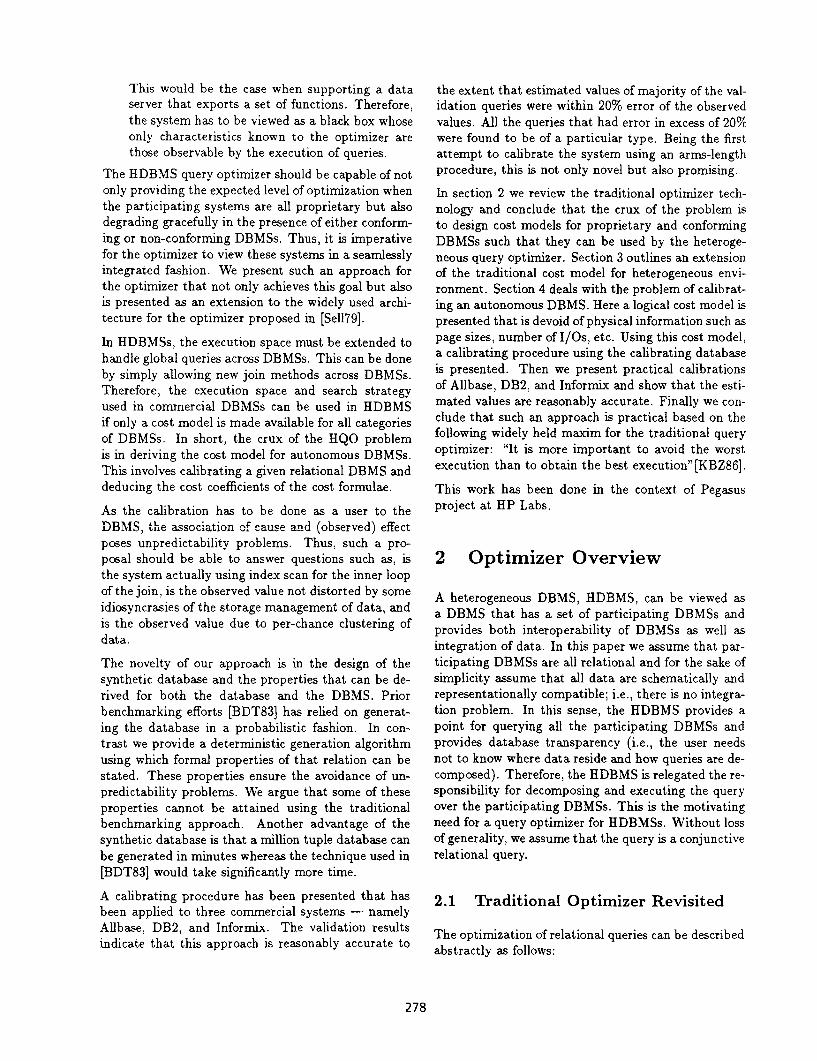
1.1. select Cl from R, where Cl = c 1.2. select C3 from R, where C3 = c 1.3. select Ch from R, where Cd = c 2.1. select Cz from R, where Cl = c 2.2. select C’z from R, where C’s = c 2.3. select Cz from R, where C, = c 3.1. select Cz from R, where Cz < c 3.2. select C’s from R, where C’s < c 3.3. select CS from R, where CS < c 4.1. select Cl from R, where Cz < c 4.2. select Cl from R, where C’s < c 4.3. select Cl from R, where CS < c

/pEx Allbase 1 DB2

1.9 1 0.60 ts/105 0.000175 1.35 0.0007 0.00036 1.35 0.0007 0.0007 1.35 0.0007

ts/1.4*106 0.0003 1.2 0.0003 0.0003 1.2 0.0003 0.0003 1.2 0.0003

Figure 4: Calibration Queries for Table & .014 - .024 1 .007 - .009

Note:

the system parameters were not altered. l ts is the tuple size (in bytes). l CS2,i varies slightly on table size.

There are 16 relations used in these calibrations as shown in Figure 3. Each type of relation was instan- tiated with two sizes of tuples and the smaller tuple relation was duplicated. This duplication is because the join queries needed two identical relations. Rela- tions of type RIO, R13, Rls and R17 were used in the calibration of Allbase and Informix whereas relations of type R13, R15, R17 and Rzo were used in the calibration of DB2. This choice is because of the availability of disk space. The calibration procedure is identical.

Figure 5: Allbase, DB2, and Informix Cost Formulae

The actual queries used in the calibration are given in Figure 4, where R,, is a table of cardinality 2” and c is a constant which determines the selectivity. For each type of query against R,,, a set of queries with selectivity 2-” (i=1,2,...,n) are constructed and observed.

For each query the elapsed time in the DBMS is recorded. For DB2, the elapsed time is defined as class 2 elapse time (see [IBM-DBS]). For Allbase and In- formix, it is calculated by subtracting the start times- tamp (when the query is received) from the end times- tamp (when the result has been sent out). In all DBMSs the queries were posed after flushing all the buffers to eliminate the distortion due to buffering. Each query is issued 30 times and the average elapse time is calculated. Except few cases, relative error between actual data and average value is within 5% with confidence coefficient of 95%. Thus, the repeatability of the observation was assured.

Figure 7. This corroborates two facts: 1) DB2 access to index only queries are not sensitive to size of the relation; 2) the approximation used for CSli, is not affecting the accuracy very much. As it can be seen, the error is quite small and this was true for all tests using the queries above.

To explore the effect of multiple selection and projection clauses, we modify and rerun the twelve basic queries on DB2. The new queries have upto five predicates and return upto five attributes. The following are two example queries.

select C1,C2,C3,CqlC5 from Iln where C5<c

Select C5 from Rn where C5<c & Cl>0 & Cz>O & ($20 & C4>0

From these, the coefficients for the cost formulae for Allbase, DB2, and Informix can be deduced. Least square fitting algorithm was used to minimize the er- rors and estimate the coefficients, These are reported in Figure 5. The elapsed time for queries of the type 3.1 running on DB2 for relations RI3 and R17 along with the estimated time by the cost formula, which is independent of the size of the relation, are shown in

Note that in the second query, the ‘2’ predicates are true for all tuples. This guarantees that they are checked for those and only those tuples that have suc- ceeded with the first (original) predicate.

The result of the experiments shows that in all cases, the differences are within 10%. It seems to suggest that the cost of projecting additional columns is negligible once the tuple is in the memory and the cost to check predicates is also minimal comparing to other processing costs (e.g., I/O).

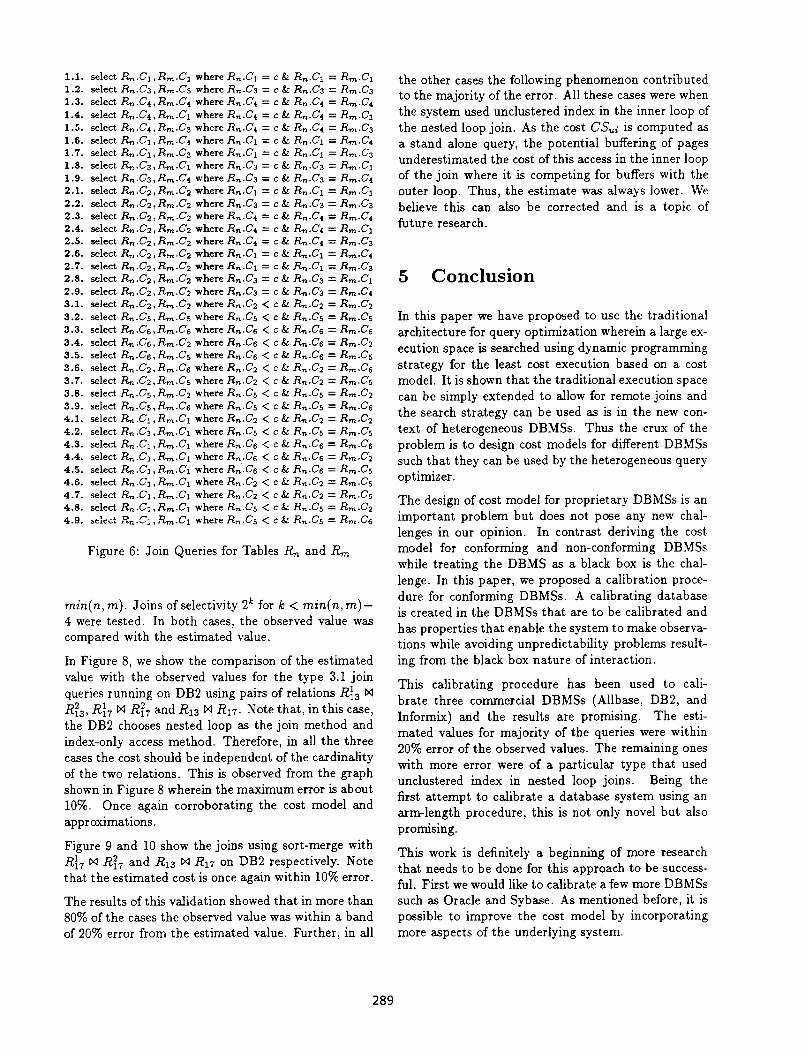
The above cost formulae were also validated using the 36 types of join queries shown in Figure 6. Queries of type 1.1-2.9 return 22*i tuples depending on constant c, where i = O,l,..., n. In this validation, joins of selectivity 22*k for k < (n - 4) were tested. Queries of type 3.1-4.9 return 2’ tuples depending on c, where i 6

Informix

0.06 (168+ts)/7*105 0.00045 0.06 0.001 0.001 0.06 0.001 0.001 0.06 0.001 .OOl - .002

288

1.1. select &,.CI, R,.Cl where R,.CI = c & R,,.Cl = R,.CI 1.2. select R,.C3, R,.C3 where R,.C3 = c & R,.C3 = Rm.C3 1.3. select R,,.C4,R,.C4 where Rn.C4 = c & Rn.C4 = R,.C4 1.4. select &.C4, R,.Cl where R,.C4 = c & R,.C4 = R,.Cl 1.5. select R,,.C4, R,.C3 where Rn.C4 = c & R,.C4 = R,,,.C3 1.6. select R,,.Cl,R,.C4 where Rn.Cl = c & R,.Cl = R,.C4 1.7. select R,,.C,,R,.C3 where Rn.4 = c & Rn.C1 = Rm.C3 1.8. select R,,.C3,Rm.C1 where Rn.C3 = c & Rn.C3 = R,.Cl 1.9. select R,,.C3, Rm.C4 where Rn.C3 = c & R,.C3 = R,.C4 2.1. select &.C2, Rm.C2 where Rn.Cl = c & R,.Cl = Rm.Cl 2.2. select R,,.C2,Rm.C2 where Rn.C3 = c & Rn.C3 = Rm.C3 2.3. select R.,,.C2, Rm.C2 where R,.G = c & Rn.C4 = Rm.C4

2.4. select &.C2, R,.C2 where Rn.C4 = c & R,.C4 = R,.Cl 2.5. select R,,.C2,R,.C2 where Rn.C4 = c & Rn.C4 = R,.C3

2.6. select R,,.C2, R,.C2 where R,.CI = c & R,.Cl = R,.C4 2.7. select R,,.C2,R,.C2 where R,.Cl = c & Rn.C1 = Rm.C3 2.8. select R,,.Cz,R,.Cz where Rn.C3 = c & Rn.C3 = R,.Cl 2.9. select R,,.C2,Rm.C2 where R,.C3 = c & Rn.C3 = R,.C4

3.1. select R,,,C2,Rm.C2 where Rn.C2 < c & R,.C2 = Rm.C2 3.2. select R,,.Cs,R,.Cs where R,.Cs < c & R,.Cs = Rm.Cs 3.3. select R,,.Cc,R,.Cg where Rn.Cs < c & Rn.Ce = R,.Cs 3.4. select I&,.&., Rm.C2 where R,.Cs < c & Rn.C% = R,.C2

3.5. select R,,.C6,R,.C5 where R,.Cs < c & Rn.C6 = R,.C5 3.6. select&,.C2,R,.,,.C6 where R,.C2 < c& R,.C2 =%-,.C6

3.7. select R,,.C2, R,.Cs where Rn.C2 < c & R,.C2 = R,.Cs

3.8. select F&,.(75, R,.C2 where Rn.Cs < c & Rn.C3 = R,.C2 3.9. select &.Cs, Rm.C6 where Rn.C5 < c & R,.Cs = R,.Cs 4.1. select R,,.Cl, R,.Cl where Rn.C2 < c & Rn.C2 = R,.C2 4.2. select R,,.Cl,R,.Cl where %.CS < c & h.C5 = Rm.Cs 4.3. select R,,.Cl,Rm.C~ where Rn.Cs < c& Rn.Ce = Rm.Cs 4.4. select &,.CI , R,.Cl where R,.C6 < c & R,.Cs = R,.C2 4.5. select R,,.CI ,R,.Cl where Rn’.Cs < c & R,.Cs = R,.Cs 4.6. select R,,.CI,R~.CI where SC2 < c 8~ JL.C2 = %.CS 4.7. select I&,.Cl, R,.Cl where R,.C2 < c & Rn.C2 = R,.Cs 4.8. select R,,.Cl, R,.Cl where R,.Cs < c & Rn.C3 = R,.C2 4.9. aekit Rn.Ci,a m 9 .Cl where Rn.C5 < c & Rn.Cs = Rm.Ce

Figure 6: Join Queries for Tables R,, and R,,,

min(n, m). Joins of selectivity 2’ for Ic < min(n, m)- 4 were tested. In both cases, the observed value was compared with the estimated value.

In Figure 8, we show the comparison of the estimated value with the observed values for the type 3.1 join queries running on DB2 using pairs of relations Ri3 W Rf3, Ri7 W Rf7 and RI3 W R17. Note that, in this case, the DB2 chooses nested loop as the join method and index-only access method. Therefore, in all the three cases the cost should be independent of the cardinality of the two relations. This is observed from the graph shown in Figure 8 wherein the maximum error is about 10%. Once again corroborating the cost model and approximations.

Figure 9 and 10 show the joins using sort-merge with R:, W Rf7 and RI3 W RI7 on DB2 respectively. Note that the estimated cost is once again within 10% error.

The results of this validation showed that in more than 80% of the cases the observed value was within a band of 20% error from the estimated value. Further, in all

the other cases the following phenomenon contributed to the majority of the error. All these cases were when the system used unclustered index in the inner loop of the nested loop join. As the cost C’Sui is computed as a stand alone query, the potential buffering of pages underestimated the cost of this access in the inner loop of the join where it is competing for buffers with the outer loop. Thus, the estimate was always lower. We believe this can also be corrected and is a topic of future research.

5 Conclusion

In this paper we have proposed to use the traditional architecture for query optimization wherein a large execution space is searched using dynamic programming strategy for the least cost execution based on a cost model. It is shown that the traditional execution space can be simply extended to allow for remote joins and the search strategy can be used as is in the new context of heterogeneous DBMSs. Thus the crux of the problem is to design cost models for different DBMSs such that they can be used by the heterogeneous query optimizer.

The design of cost model for proprietary DBMSs is an important problem but does not pose any new chal- lenges in our opinion. In contrast deriving the cost model for conforming and non-conforming DBMSs while treating the DBMS as a black box is the chal- lenge. In this paper, we proposed a calibration procedure for conforming DBMSs. A calibrating database is created in the DBMSs that are to be calibrated and has properties that enable the system to make observations while avoiding unpredictability problems resulting from the black box nature of interaction.

This calibrating procedure has been used to calibrate three commercial DBMSs (Allbase, DB2, and Informix) and the results are promising. The estimated values for majority of the queries were within 20% error of the observed values. The remaining ones with more error were of a particular type that used unclustered index in nested loop joins. Being the first attempt to calibrate a database system using an arm-length procedure, this is not only novel but also promising.

This work is definitely a beginning of more research that needs to be done for this approach to be success- ful. First we would like to calibrate a few more DBMSs such as Oracle and Sybase. As mentioned before, it is possible to improve the cost model by incorporating more aspects of the underlying system.

289

D. naps* TlY w nap** Tlr (in l c0n4) (In •~cona

2.30 210

210 24s

230 240

2m 2s

210 2%

200 2.15

190 2.u)

II0

1.70 23s

1.60 w

150 2u

1.M 220

1.30 21s

130 210

1.10 2w

1.00

0.00 1.00 200 3.00 4.00 0.00 moo am.00 3oam yx).w sm.00

21.60

2I10

2I.20

21.m

21 IO

2760

2740

2120

2700

24.u)

2460

26.ro

26.20

26.00

n.uJ

Y.60

n.yI

2.5.20

2s.00 0.00 200 4.00 6oD I.m

I Of mp1r Dmcurn.4 x low

2.530

n.00

24.m

24.60

24.40

24.20

2400

23Io

2360

13.40

23.20

23.00

2240

22.0

PO

pzo

2200

2l.W 0.00 2oQ 4.m am 1.m

t Of Tu91r D.turnd x 1000

i-w- 10. dm ’ bum RI>. I,, rbm R,,.C.<c ud Rt, C.= Rtr C.

290

Quantifying the effect of buffering on unclustered iildex is an important extension. As mentioned before, almost all the queries that had significant error could be argued to be due to this problem. Inferring de facto clustering from the data, such as Cz in the database would be quite useful. Sys- tems such as DB2 have knowledge of the degree of clustering for this column to be 100% and therefore may use it. In general, such information can still be used to interpolate the cost of ‘less clustered’ data. Detecting when an index scan switches to sequential scan for an unclustered index is an important information if this access method is used in a nested loop. As the system may be using some rule of thumb for the switch, the HDBMS optimizer should know the point of transition.

Finally the approach proposed here was in the context of a particular cost model. It should be obvious to the reader that even if the cost model is changed the approach can still be used to devise a new procedure. Thus, we feel the process of designing a synthetic database in a deterministic manner has merit.

Using the knowledge of the proposal here for conforming DBMSs, it is possible to extrapolate an approach for the non-conforming DBMSs. We are developing a single invocation and execution model for DBMSs in all three categories so that the query optimization process developed in this paper can be extended to cover non-conforming DBMSs. To serve the purpose, we plan to integrate some widely used non-conforming DBMSs such as IMS, VSAM and Unix applications. The calibration procedure may need to be enhanced to measure DBMSs of this category.

We also plan to explore issues of post query optimization such as dynamic reconfiguration of execution plan at run time. This is important, especially in HDBMSs, because it is difficult (and sometimes im- possible) to get accurate cost formulae. Other related issues include reduction of invocations to participating DBMSs, cross site data buffering, new global join methods, etc. These are topics of future research.

Acknowledgements

We wish to acknowledge the following people in HP Corpo- rate Computing and Services for their help in our calibration. Mike Wang and Arthur Walasek of SOLID project provided accesses to DB2 and Informix. Charlene Yoshizu, Jeff Litalien, and Kim Iverson provided considerable system support and patience while our calibration consumed vast amounts of their resources.

References

[AetalSl]

[BDT83]

[CGKSO]

[CP84]

[D&51

[GHK92]

Ahmed, R., et al, “The Pegasus Heteroge- neous Multidatabase System”, IEEE Com- puter Magazine, Vol. 24, No. 12, 1991.

Bitton, D., D. Dewitt, and C. Turbyfill, “Benchmarking Database Systems: A Sys- tematic approach” Proc. of VLDB, 1983.

Chimenti, D., R. Gamboa, and R. Krish- namurthy, “Abstract Machine for LVL,” Proc. of EDBT, 1990.

Ceri, S. and G. Pelagat ti , Distributed Databases: Principles & Sys- terns, McGraw-Hill Book Company, 1984.

Dayal, U., “Query Processing in Multi- database System”, Query Processing in Database Systems, Edited by W. Kim, D. Reiner and D. Batory, Springer Verlag, 1985.

Ganguly, S., W. Hasan, and R. Krishna- murthy, “Query Optimization for Parallel Execution”, Proc. of SIGMOD, 1992.

[HWKSPl] Proc. of Workshop on Multidatabases and Semantic Interoperability, Tulsa, OK., Nov. 1990, Tulsa, OK.

[HWKSPS] Proc. of 1st Intl. Workshop on Interoper- ability in Multidatabase Systems, Kyoto, Japan, Apr., 1991.

[IBM-DBS] “DB2 Performance Monitor (DB2PM) Usage Guide”, Document no. GG24-3413- 00, Published by IBM Corporation, 1989.

[KBZSS]

[LS92]

[Sell791

lYK903

Krishnamurthy, R., H. Boral, and C. Zaniolo, “Optimization of Non-Recursive Q ueries,” Proc. of VLDB, 1986.

Lu, H., and M. Shan, “Global Query Optimization in Multidatabase Systems”, 1992 NFS Workshop on Heterogeneous Databases and Semantic Interoperability, 1992.

Sellinger, P.G. et al., “Access Path Selec- tion in a Relational Database Management System,” Proc. of SIGMOD, 1979.

Whang, K., and R. Krishnamurthy, “Query Optimization in a Memory-Resident Do- main Relational Calculus Database Sys- tem” TODS, Vol, 15, No. 1, 1990.

291

Query Optimization in Heterogeneous DBMS - CiteSeer

Documents

Transcript of Query Optimization in Heterogeneous DBMS - CiteSeer