Query Optimization: Chap. 15
44
Query Optimization: Chap. 15 CS634 Lecture 12 Slides based on “Database Management Systems” 3 rd ed, Ramakrishnan and Gehrke
Transcript of Query Optimization: Chap. 15

Query Optimization: Chap. 15
CS634Lecture 12
Slides based on “Database Management Systems” 3rd ed, Ramakrishnan and Gehrke

Query Evaluation Overview
SQL query first translated to relational algebra (RA)
Actually, some additional operators needed for SQL
Tree of RA operators, with choice of algorithm among
available implementations for each operator
Main issues in query optimization
For a given query, what plans are considered?
Algorithm to search plan space for cheapest (estimated) plan
How is the cost of a plan estimated?
Objective
Ideally: Find best plan
Practically:Avoid worst plans!

Evaluation Example
SELECT S.snameFROM Reserves R, Sailors SWHERE R.sid=S.sid AND
R.bid=100 AND S.rating>5
Reserves Sailors
sid=sid
bid=100 rating > 5
sname
(Simple Nested
Loops)
(On-the-fly)
(On-the-fly)
Annotated Tree

Cost Estimation
For each plan considered, must estimate:
Cost of each operator in plan tree
Depends on input cardinalities
Operation and access type: sequential scan, index scan, joins
Size of result for each operation in tree
Use information about the input relations
For selections and joins, assume independence of predicates

Query Blocks
SQL query parsed into a collection of query blocks
Blocks are optimized one at a time
Nested blocks can be treated as calls to a subroutine
One call made once per outer tuple
In some cases cross-block optimization is possible
A good query optimizer can unnest queries
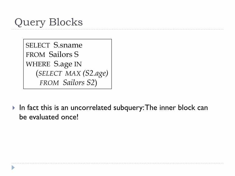
SELECT S.snameFROM Sailors SWHERE S.age IN
(SELECT MAX (S2.age)FROM Sailors S2)
Nested block
Outer block
Query Blocks
In fact this is an uncorrelated subquery: The inner block can
be evaluated once!
SELECT S.snameFROM Sailors SWHERE S.age IN
(SELECT MAX (S2.age)FROM Sailors S2)
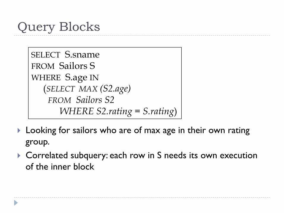
Query Blocks
Looking for sailors who are of max age in their own rating
group.
Correlated subquery: each row in S needs its own execution
of the inner block
SELECT S.snameFROM Sailors SWHERE S.age IN
(SELECT MAX (S2.age)FROM Sailors S2
WHERE S2.rating = S.rating)
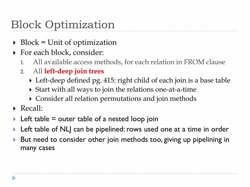
Block Optimization
Block = Unit of optimization
For each block, consider:1. All available access methods, for each relation in FROM clause
2. All left-deep join trees
Left-deep defined pg. 415: right child of each join is a base table
Start with all ways to join the relations one-at-a-time
Consider all relation permutations and join methods
Recall:
Left table = outer table of a nested loop join
Left table of NLJ can be pipelined: rows used one at a time in order
But need to consider other join methods too, giving up pipelining in many cases

Expressions
Query is simplified to a selection-projection-cross
product expression
Aggregation and grouping can be done afterwards
Optimization with respect to such expressions
Cross-product includes conceptually joins
Will talk about equivalences in a bit

Statistics and Catalogs
To choose an efficient plan, we need information about the
relations and indexes involved
Catalogs contain information such as:
Tuple count (NTuples) and page count (NPages) for each relation
Distinct key value count (NKeys) for each index, INPages
Index height, low/high key values (Low/High) for each tree index
Histograms of the values in some fields (optional)
Catalogs updated periodically
Approximate information used, slight inconsistency is ok
Databases provide tools for updating stats on demand

Size Estimation and Reduction Factors
Maximum number of tuples is cardinality of cross product
Reduction factor (RF) associated with each term reflects its
impact in reducing result size
Implicit assumption that terms are independent!
col = value has RF =1/NKeys(I), given index I on col
col1 = col2 has RF = 1/max(NKeys(I1), NKeys(I2))
col > value has RF = (High(I)-value)/(High(I)-Low(I))
Example: rating > 6 has RF = 4/10 = 0.4
SELECT attribute listFROM relation listWHERE term1 AND ... AND termk

Histograms
Most often, data values are not uniformly distributed within
domain
Skewed distributions result in inaccurate cost estimations
Histograms
More accurate statistics
Break up the domain into buckets
Store the count of records that fall in each bucket
Tradeoff
Histograms are accurate, but take some space
The more fine-grained the partition, the better accuracy
But more space required

Histogram Classification
Equiwidth
Domain split into equal-length partitions
Large difference between counts in different buckets
Dense areas not sufficiently characterized
Equidepth
Histograms “adapts” to data distribution
Fewer buckets in sparse areas, more buckets in dense areas
Used by Oracle (pg. 485)

Relational Algebra Equivalences
Why are they important?
They allow us to:
Convert cross-products to joins
Cross products should always be avoided (when possible)
Choose different join orders
Recall that choice of outer/inner influences cost
“Push-down” selections and projections ahead of joins
When doing so decreases cost

Relational Algebra Equivalences
Selections:
c cn c cnR R1 1 ... . . .
c c c cR R1 2 2 1 Commute
Cascade
Cascade property:
Allows us to check multiple conditions in same pass
Allows us to “push down” only partial conditions (when not
possible/advantageous to push entire condition)

Relational Algebra Equivalences
Projections:
a a anR R1 1 . . . Cascade
If every ai set is included in ai+1,
Example:a1 = {a,b}, a2 = {a,b,c}a2(T) has (a, b, c) columns
a1(a2(T)) has (a,b) columns, same as a1(T)

R (S T) (R S) T
Relational Algebra Equivalences
Joins:
Associative
(R S) (S R) Commute
Sketch of proof:
Show for cross product
Add join conditions as selection operators
Use cascading selections in associative case

Relational Algebra Equivalences
Joins:
Associative
Commute
Commutative property:
Allows us to choose which relation is inner/outer
Associative property:
Allows us to restrict plans to left-deep only, i.e., any query tree can be turned into a left-deep tree.
R (S T) (R S) T
(R S) (S R)

Relational Algebra Equivalences
Commuting selections with projections
Projection can be done before selection if all attributes in the
condition evaluation are retained by the projection
)()( RR acca
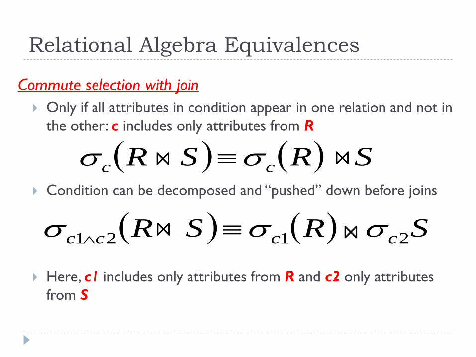
Relational Algebra Equivalences
Commute selection with join
Only if all attributes in condition appear in one relation and not in
the other: c includes only attributes from R
Condition can be decomposed and “pushed” down before joins
Here, c1 includes only attributes from R and c2 only attributes
from S
SRSR cc
SRSR cccc 2121

Relational Algebra Equivalences
Commute projection with join
Only if attributes in join condition appear in the corresponding
projection lists (so they aren’t “projected out”)
)( 2c1c SRSR aaa

System R Optimizer
Developed at IBM starting in the 1970’s
Most widely used currently; works well for up to 10 joins
Cost estimation
Statistics maintained in system catalogs
Used to estimate cost of operations and result sizes
Query Plan Space
Only the space of left-deep plans is considered
Left-deep plans allow output of each operator to be pipelined into
the next operator without storing it in a temporary relation
Cartesian products avoided

SQL Query Semantics (pg. 136, 156)
1. compute the cross product of tables in FROM
2. delete rows that fail the WHERE clause
3. project out columns not mentioned in select list or group by or having clauses
4. group rows by GROUP BY
5. apply HAVING to the groups, dropping some out
6. if necessary, apply DISTINCT
7. if necessary, apply ORDER BY
Note this all follows the order of the SELECT clauses, except for projection and DISTINCT, so it’s not hard to remember.

Single-Relation Plans

Single-Relation Plans
FROM clause contains single relation
Query is combination of selection, projection, and aggregates
(possibly GROUP BY and HAVING, but these come late in
the logical progression, so usually less crucial to planning)
Main issue is to select best from all available access paths
(either file scan or index)
Access path involves the table and the WHERE clause
Another factor is whether the output must be sorted
E.g., GROUP BY requires sorting (or hashing)
Sorting may be done as separate step, or using an index if an
indexed access path is available

Plans Without Indexes
Only access path is file scan
Apply selection and projection to each retrieved tuple
Projection may or may not use duplicate elimination, depending on whether there is a DISTINCT keyword present
GROUP BY:
Write out intermediate relation after selection/projection
(or pipeline into sort)
Sort intermediate relation to create groups
Apply aggregates on-the-fly per each group
HAVING also performed on-the-fly, no additional I/O needed
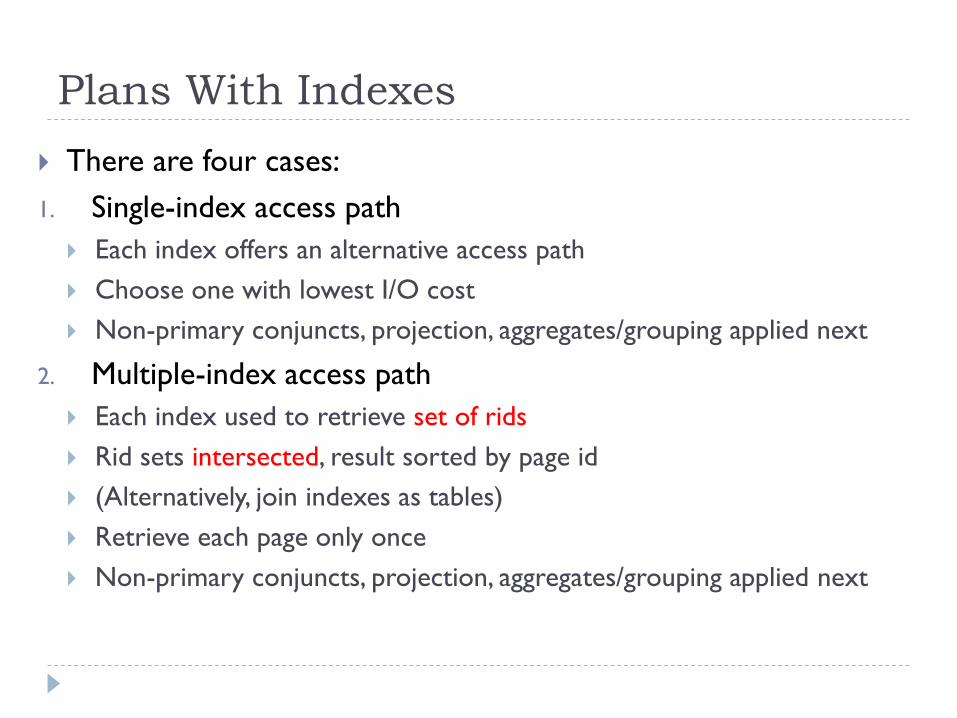
Plans With Indexes
There are four cases:
1. Single-index access path
Each index offers an alternative access path
Choose one with lowest I/O cost
Non-primary conjuncts, projection, aggregates/grouping applied next
2. Multiple-index access path
Each index used to retrieve set of rids
Rid sets intersected, result sorted by page id
(Alternatively, join indexes as tables)
Retrieve each page only once
Non-primary conjuncts, projection, aggregates/grouping applied next

Plans With Indexes (contd.)
3. Tree-index access path: extra possible use…
If GROUP BY attributes prefix of tree index, retrieve tuples in
order required by GROUP BY
Apply selection, projection for each retrieved tuple, then aggregate
Works well for clustered indexes
Example: With tree index on rating
SELECT count(*), max(age)FROM Sailors SGROUP BY rating

Plans With Indexes (contd.)
3. Index-only access path
If all attributes in query included in index, then there is no need to
access data records: index-only scan
If index matches selection, even better: only part of index examined
Does not matter if index is clustered or not!
If GROUP BY attributes prefix of a tree index, no need to sort!
Example: With tree index on rating
Note count(*) doesn’t require access to row, just RID.
SELECT max(rating),count(*)FROM Sailors S

Example Schema
Similar to old schema; rname added
Reserves:
40 bytes long tuple, 100K records, 100 tuples per page, 1000 pages
Sailors:
50 bytes long tuple, 40K tuples, 80 tuples per page, 500 pages
Assume index entry size 10% of data record size
Sailors (sid: integer, sname: string, rating: integer, age: real)Reserves (sid: integer, bid: integer, day: dates, rname: string)
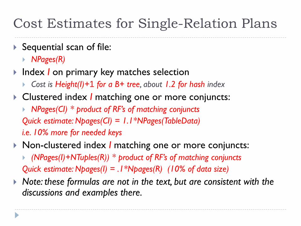
Cost Estimates for Single-Relation Plans
Sequential scan of file:
NPages(R)
Index I on primary key matches selection
Cost is Height(I)+1 for a B+ tree, about 1.2 for hash index
Clustered index I matching one or more conjuncts:
NPages(CI) * product of RF’s of matching conjuncts
Quick estimate: Npages(CI) = 1.1*NPages(TableData)
i.e. 10% more for needed keys
Non-clustered index I matching one or more conjuncts:
(NPages(I)+NTuples(R)) * product of RF’s of matching conjuncts
Quick estimate: Npages(I) = .1*Npages(R) (10% of data size)
Note: these formulas are not in the text, but are consistent with the discussions and examples there.

Example
File scan: retrieve all 500 pages
Clustered Index I on rating
(1/NKeys(I)) * (NPages(CI)) = (1/10) * (50+500) pages
Unclustered Index I on rating
(1/NKeys(I)) * (NPages(I)+NTuples(S)) = (1/10) * (50+40000) pages
SELECT S.sidFROM Sailors SWHERE S.rating=8
Note: One rating value owns a fraction
(1/10) of the index at all levels, so
#pages accessed = (1/10) Npages(CI)
Or (1/10) Npages(I)

Multiple-Relation Plans

Queries Over Multiple Relations
In System R only left-deep join trees are considered
In order to restrict the search space
Left-deep trees allow us to generate all fully pipelined plans
Intermediate results not written to temporary files.
Not all left-deep trees are fully pipelined (e.g., sort-merge join)
BA
C
D
BA
C
D
C DBA
Left-deep

Enumeration of Left-Deep Plans
Among all left-deep plans, we need to determine:
the order of joining relations
the access method for each relation
the join method for each join
Enumeration done in N passes (if N relations are joined):
Pass 1: Find best 1-relation plan for each relation
Pass 2: Find best way to join result of each 1-relation plan (as outer) to another relation - result is the set of all 2-relation plans
Pass N: Find best way to join result of a (N-1)-relation plan (as outer) to the N’th relation - result is the set of all N-relation plans
Speed-up computation using dynamic programming (remember details of good plans to avoid recalc)

For each subset of relations, retain only:
Cheapest plan overall, plus
Cheapest plan for each interesting order of the tuples
Interesting order: order that allows execution of GROUP BY
without requiring an additional step of sorting, aggregates
Avoid Cartesian products if possible
An N-1 way plan is not combined with an additional relation
unless there is a join condition between them
Exception is case when all predicates in WHERE have been used
up (i.e., query itself requires a cross-product)
Ex: select … from T1, T2, T3 where T1.x = T2.x
Only one join condition, 3 tables, so end up with cross product
Enumeration of Left-Deep Plans (contd.)

Cost Estimation for Multi-Relation Plans
Two components:
1. Size of intermediate relations Maximum tuple count is the product of the cardinalities of relations in
the FROM clause
Reduction factor (RF) associated with each condition term
Result cardinality estimate = Max # tuples * product of all RF’s
Example query on next slide: Result cardinality estimate = (40K*100K) * ((1/100)*(5/10)*(1/40K)) = 500
This means we estimate the query returns 500 rows as its result
It is not a “cost” calculation
Here 1/40K = RF of join condition, 1/100 assumes 100 boats.
2. Cost of each join operator Depends on join method

Example
SELECT S.snameFROM Sailors S, Reserves RWHERE S.sid=R.sid AND S.rating>5 AND R.bid=100
Reserves Sailors
sid=sid
bid=100 rating > 5
sname
Reserves Sailors
sid=sid
bid=100 rating > 5
sname
But this is not left-deep!

Pass 1 Single-relation plans
Sailors
B+ tree matches rating>5
Most selective access path
But index unclustered!
Sometimes may prefer scan
Reserves
B+ tree on bid matches selection bid=100
Cheapest plan for this table
Note: Here we are evaluating plans as candidates for the leftmost spot in the final plan
Result of Pass 1: One plan for each table.
Sailors:Unclustered B+ tree on ratingUnclustered Hash on sid
Reserves:Unclustered B+ tree on bid
Example

Example
Pass 2
Consider each plan retained from Pass 1 as the outer, and how
to join it with the (only) other relation
Sailors outer, Reserves inner
No index matches join condition, this could be done as block
nested loop
Reserves outer, Sailors inner
Since we have hash index on sid for Sailors, this could be a
cheap plan using an indexed nested loop
This would mean S.rating>5 is done after join.
Also see discussion of this on pg. 412, point 3
End up with left-deep plan.

Example, cont. (pipelining not in book)
Also need to check sort-merge join
But that requires materialization of input tables, an extra
expense (or use pipelining into sort)
Need to cost all three competing plans, choose least
expensive
Note that left-deep plans assume nested-loop joins are in
use, so may miss good hash join plans
Note on pg. 500: Oracle considers non-left-deep plans to
better utilize hash joins.

Nested Queries
Nested block is optimized independently, with the outer tuple
considered as providing a selection condition
Outer block is optimized with the cost of “calling” nested
block computation taken into account
Implicit ordering of these blocks means that some good
strategies are not considered
The non-nested version of the query is typically optimized better

Nested Queries
SELECT S.snameFROM Sailors SWHERE EXISTS
(SELECT *FROM Reserves RWHERE R.bid=103 AND R.sid=S.sid)
Equivalent non-nested query:
SELECT S.snameFROM Sailors S, Reserves RWHERE S.sid=R.sid
AND R.bid=103