Query Compiler: 16.7 Completing the Physical Query-Plan

CS257 Spring 2009Professor Tsau Lin

Student: Suntorn Sae-EungID: 212

Outline

16.7 Completing the Physical-Query-PlanI. Choosing a Selection Method

II. Choosing a Join Method

III. Pipelining Versus Materialization

IV. Pipelining Unary Operations

V. Pipelining Binary Operations

Before complete Physical-Query-Plan

A query previously has been Parsed and Preprocessed (16.1)Converted to Logical Query Plans (16.3) Estimated the Costs of Operations (16.4)Determined costs by Cost-Based Plan

Selection (16.5)Weighed costs of join operations by

choosing an Order for Joins

16.7 Completing the Physical-Query-Plan

3 topics related to turning LP into a complete physical plan

1. Choosing of physical implementations such as Selection and Join methods

2. Decisions regarding to intermediate results (Materialized or Pipelined)

3. Notation for physical-query-plan operators

I. Choosing a Selection Method (A)

Algorithms for each selection operators1. Can we use an created index on an

attribute? If yes, index-scan. Otherwise table-scan)

2. After retrieve all condition-satisfied tuples in (1), then filter them with the rest selection conditions

Choosing a Selection Method(A) (cont.)

Recall Cost of query = # disk I/O’s How costs for various plans are estimated from σC(R) operation

1. Cost of table-scan algorithm

a) B(R) if R is clustered

b) T(R) if R is not clustered

2. Cost of a plan picking an equality term (e.g. a = 10) w/ index-scan

a) B(R) / V(R, a) clustering index

b) T(R) / V(R, a) nonclustering index

3. Cost of a plan picking an inequality term (e.g. b < 20) w/ index-scan

a) B(R) / 3 clustering index

b) T(R) / 3 nonclustering index

Example

Selection: σx=1 AND y=2 AND z<5 (R)

- Where paremeters of R(x, y, z) are :

T(R)=5000, B(R)=200,

V(R,x)=100, and V(R, y)=500

- Relation R is clustered

- x, y have nonclustering indexes, only index on z is clustering.

Example (cont.)

Selection options:1. Table-scan filter x, y, z. Cost is B(R) = 200 since

R is clustered.2. Use index on x =1 filter on y, z. Cost is 50 since

T(R) / V(R, x) is (5000/100) = 50 tuples, index is not clustering.

3. Use index on y =2 filter on x, z. Cost is 10 since T(R) / V(R, y) is (5000/500) = 10 tuples using nonclustering index.

4. Index-scan on clustering index w/ z < 5 filter x ,y. Cost is about B(R)/3 = 67

Example (cont.)

Costsoption 1 = 200 option 2 = 50 option 3 = 10 option 4 = 67

The lowest Cost is option 3. Therefore, the preferred physical plan

1. retrieves all tuples with y = 2 2. then filters for the rest two conditions (x, z).

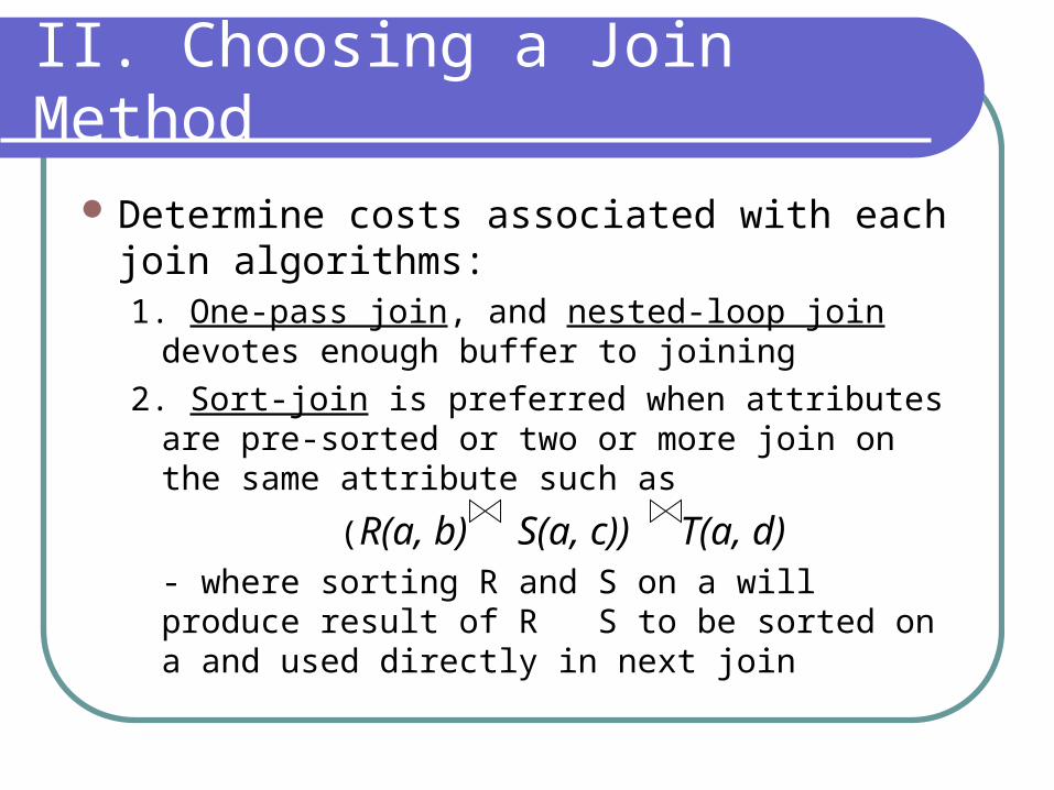
II. Choosing a Join Method

Determine costs associated with each join algorithms: 1. One-pass join, and nested-loop join devotes

enough buffer to joining

2. Sort-join is preferred when attributes are pre-sorted or two or more join on the same attribute such as

(R(a, b) S(a, c)) T(a, d) - where sorting R and S on a will produce result of R S to be sorted on a and used directly in next join

3. Index-join for a join with high chance of using index created on the join attribute such as R(a, b) S(b, c)

4. Hashing join is the best choice for unsorted or non-indexing relations which needs multipass join.

Choosing a Join Method (cont.)

III. Pipelining Versus Materialization

Materialization (naïve way)

store (intermediate) result of each operations on disk

Pipelining (more efficient way)

Interleave the execution of several operations, the tuples

produced by one operation are passed directly to the

operations that used it

store (intermediate) result of each operations on buffer, which

is implemented on main memory

Unary = a-tuple-at-a-time or full relationselection and projection are the best

candidates for pipelining.

IV. Pipelining Unary Operations

R

In buf Unaryoperation

Out buf

In buf Unaryoperation

Out buf

M-1 buffers

Pipelining Unary Operations (cont.)

Pipelining Unary Operations are implemented by iterators

V. Pipelining Binary Operations

Binary operations : , , - , , xThe results of binary operations can also

be pipelined.Use one buffer to pass result to its

consumer, one block at a time.The extended example shows tradeoffs

and opportunities

Example

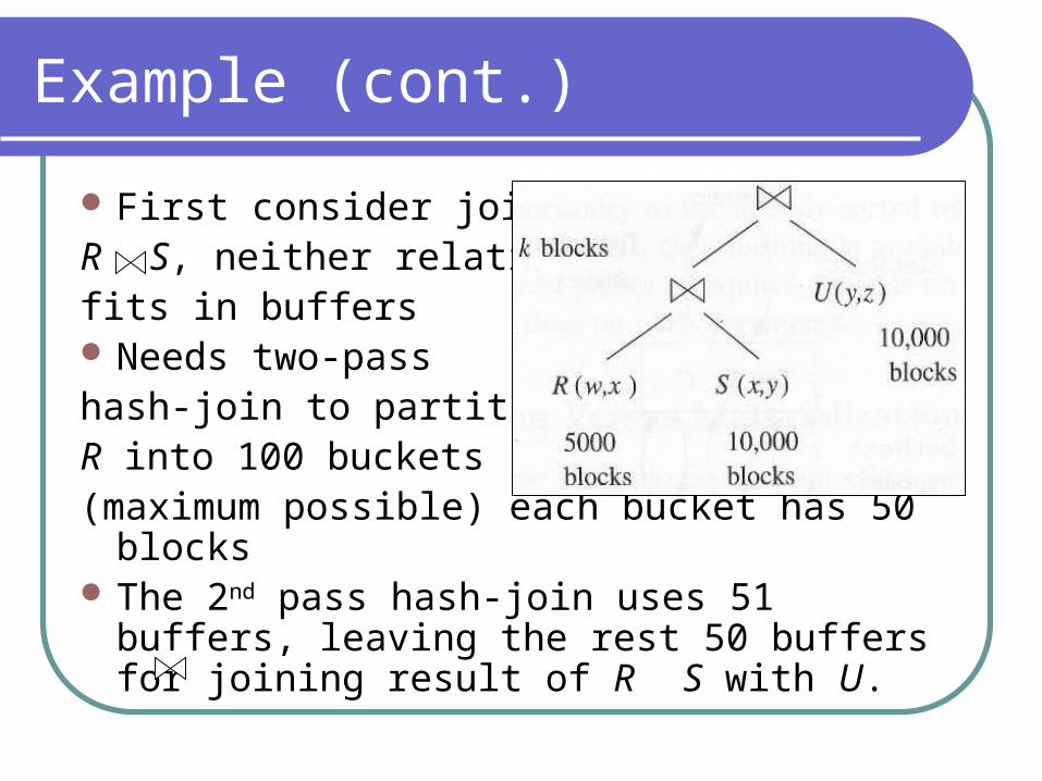
Consider physical query plan for the expression

(R(w, x) S(x, y)) U(y, z) Assumption

R occupies 5,000 blocks, S and U each 10,000 blocks.

The intermediate result R S occupies k blocks for some k.

Both joins will be implemented as hash-joins, either one-pass or two-pass depending on k

There are 101 buffers available.

Example (cont.)

First consider join R S, neither relations fits in buffers Needs two-pass hash-join to partition R into 100 buckets (maximum possible) each bucket has 50 blocks The 2nd pass hash-join uses 51 buffers, leaving

the rest 50 buffers for joining result of R S with U.

Example (cont.)

Case 1: suppose k 49, the result of R S occupies at most 49 blocks.

Steps 1. Pipeline in R S into 49 buffers

2. Organize them for lookup as a hash table

3. Use one buffer left to read each block of U in turn

4. Execute the second join as one-pass join.

Example (cont.)

The total number of I/O’s is 55,000 45,000 for two-pass

hash join of R and S 10,000 to read U for

one-pass hash join of (R S) U.

Example (cont.)

Case 2: suppose k > 49 but < 5,000, we can still pipeline, but need another strategy which intermediate results join with U in a 50-bucket, two-pass hash-join. Steps are:

1. Before start on R S, we hash U into 50 buckets of 200 blocks each.

2. Perform two-pass hash join of R and U using 51 buffers as case 1, and placing results in 50 remaining buffers to form 50 buckets for the join of R S with U.

3. Finally, join R S with U bucket by bucket.

Example (cont.)

The number of disk I/O’s is:20,000 to read U and write its tuples into

buckets45,000 for two-pass hash-join R Sk to write out the buckets of R Sk+10,000 to read the buckets of R S and U

in the final joinThe total cost is 75,000+2k.

Example (cont.)

Compare Increasing I/O’s between case 1 and case 2k 49 (case 1)

Disk I/O’s is 55,000k > 50 5000 (case 2)

k=50 , I/O’s is 75,000+(2*50) = 75,100k=51 , I/O’s is 75,000+(2*51) = 75,102k=52 , I/O’s is 75,000+(2*52) = 75,104

Notice: I/O’s discretely grows as k increases from 49 50.

Example (cont.)

Case 3: k > 5,000, we cannot perform two-pass join in 50 buffers available if result of R S is pipelined. Steps are

1. Compute R S using two-pass join and store the result on disk.

2. Join result on (1) with U, using two-pass join.

Example (cont.)

The number of disk I/O’s is:45,000 for two-pass hash-join R and Sk to store R S on disk30,000 + k for two-pass join of U in R S

The total cost is 75,000+4k.

Example (cont.)

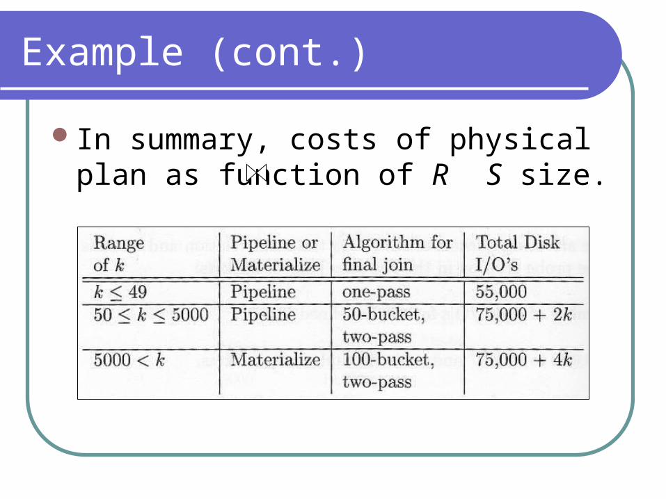
In summary, costs of physical plan as function of R S size.

Questions & Answers

For your attention

Reference

[1] H. Garcia-Molina, J. Ullman, and J. Widom, “Database System: The Complete Book,” second edition: p.897-913, Prentice Hall, New Jersy, 2008