QUBE – Array Programming with Dependent Types · to perform any dynamic checks such as array...
161
Aus dem Institut für Softwaretechnik und Programmiersprachen der Universität zu Lübeck Direktor: Prof. Dr. Martin Leucker Q UBE – Array Programming with Dependent Types Inauguraldissertation zur Erlangung der Doktorwürde der Universität zu Lübeck Aus der Sektion Informatik/Technik vorgelegt von Dipl.-Inf. Kai Trojahner aus Flensburg Lübeck 2011
Transcript of QUBE – Array Programming with Dependent Types · to perform any dynamic checks such as array...
Aus dem Institut für Softwaretechnik und Programmiersprachender Universität zu Lübeck
Direktor: Prof. Dr. Martin Leucker
QUBE – Array Programming withDependent Types
Inauguraldissertationzur
Erlangung der Doktorwürdeder Universität zu Lübeck
Aus der Sektion Informatik/Technik
vorgelegt von
Dipl.-Inf. Kai Trojahneraus Flensburg
Lübeck 2011

1. Berichterstatter: Prof. Dr. Till Tantau
2. Berichterstatter: Dr. Clemens Grelck
Vorsitzender des Prüfungsausschusses: Prof. Dr. Martin Leucker
Tag der mündlichen Prüfung: 1. Juni 2011

Walter Dosch
1947 – 2010


Zusammenfassung
Arrayprogrammiersprachen wie APL oder MATLAB verwenden multidimensio-nale Arrays als grundlegende Datenstrukturen. Rank-generische Operationensind gleichermaßen auf Vektoren, Matrizen, und höherdimensionale Arrays an-wendbar. Bei vielen Operationen unterliegen die Operanden jedoch spezifischenEinschränkungen bezüglich der Typen ihrer Elemente und ihrer Form. Beispiels-weise überprüft die MATLAB-Operation A + B zur Laufzeit, ob beide Operan-den die gleiche Form haben und ob die Addition der Elemente definiert ist. ImFalle einer Anwendung auf inkompatible Operanden wird die Ausführung desgesamten Programms abgebrochen.In dieser Arbeit stelle ich die Programmiersprache QUBE vor, welche die statischeVerifikation von Arrayprogrammen unterstützt, so dass Fehler schon währendder Übersetzung entdeckt werden. Dazu verwendet QUBE abhängige Typen, diesowohl den Elementtyp als auch die Form eines Arrays beschreiben. Weil Ar-rays unterschiedlicher Form verschiedene Typen haben, können die erlaubtenArgumente einer Funktion genau angegeben werden. Das Typsystem kann Ele-menttypfehler, Formfehler und Indexfehler ausschließen.Als formales Modell von QUBE definiere ich die Kernsprache QUBECORE. Eineoperationelle Semantik definiert die korrekte Auswertung von QUBECORE unddie möglichen Laufzeitfehler. Das Typsystem von QUBECORE wird durch eineMenge von Ableitungsregeln für wohlgeformte Typen, die Subtyprelation und dieTypüberprüfung von Ausdrücken beschrieben. Ich beweise, dass bei der Auswer-tung von wohlgetypten Ausdrücken keine Laufzeitfehlern auftreten können.Um zu untersuchen, wie abhängige Typen genutzt werden können, um aus rank-generischen Spezifikationen effiziente Programme zu erzeugen, habe ich zusam-men mit meinen Studenten einen Übersetzer für QUBE konstruiert. Der Über-setzer verwendet für die Typüberprüfung einen Theorembeweiser für das SMTProblem. Da QUBE-Programme statisch verifiziert werden, brauchen sie keinedynamischen Tests wie etwa Bereichstests durchzuführen. MultidimensionaleArrays werden als reine Sequenzen von Daten ohne Typannotationen oder Form-deskriptoren repräsentiert. Erste Experimente zeigen, dass für einige interes-sante Benchmarks QUBE-Programme ähnlich schnell wie C-Programme sind.
v

Abstract
Array programming languages such as APL or MATLAB use multidimensional ar-rays as the primary data structures. Rank-generic operations apply transparentlyto vectors, matrices, and arrays with an even higher rank. Often, these opera-tions require that the ranks, shapes, and the elements of their arguments satisfycertain constraints. For example, in MATLAB, the element-wise addition A + Bdynamically checks that both arrays have the same shape. In case of an improperapplication, the entire program aborts with an error message.In this thesis, I present QUBE, a new programming language that checks arrayprograms at compile time, such that errors are detected before a program is run.For this purpose, QUBE employs an advanced type system based on dependenttypes, i. e., types that depend on values. Since dependent types distinguish be-tween arrays of different shapes, the allowed arguments of a function can beprecisely characterised. The type system is sufficiently expressive to staticallyrule out base type errors, shape errors, and even array boundary violations.As a formal model of QUBE, I define the core language QUBECORE. An opera-tional semantics defines both the proper evaluation of QUBECORE as well as thepotential run-time errors. The type system of QUBECORE is described by a setof inference rules that formally specify well-formed types, the subtype relation,and type checking of QUBECORE expressions. I provide a proof that QUBECORE istype-safe, i. e., evaluating a well-typed expression will not cause a run-time error.To explore how the power of dependent types can be harnessed to generate ef-ficient code from rank-generic programs, I, with help from my students, haveconstructed a compiler for QUBE. The compiler performs type checking in col-laboration with an SMT solver. Due to static verification, programs do not needto perform any dynamic checks such as array bounds checks. Moreover, multidi-mensional arrays are represented as mere sequences of data without additionaltype tags or shape descriptors. Early experiments show that for some interestingbenchmarks, the run-time performance of QUBE programs is comparable withhandwritten C code.
vii

Acknowledgements
I dedicate this thesis to Walter Dosch, who was my initial thesis advisor. When Iwas a freshman at the University of Lübeck, he introduced me to the wonderfulworld of functional programming. For my dissertation, he encouraged me todevelop my own programming language, then called the Lübeck Array Language,and patiently guided me through my research. Walter Dosch passed away far toosoon in August 2010.In July 2010, Till Tantau graciously consented to take care of me in the finalstages of my thesis. I especially thank him for taking over and providing helpfulcomments as well as inspiring discussions.A great deal of thanks goes to Clemens Grelck who initiated me to the SAC arrayprogramming language and compiler project. He supervised my diploma thesisand motivated me to make my own contributions to the field.Several students helped me implement the QUBE compiler in its various incarna-tions. Without Florian Büther, the compiler surely wouldn’t be here, but alsoMarkus Weigel, Johannes Blume, and Sebastian Hungerecker made valuablecontributions.I thank my colleagues from the Institute of Software Technology and Program-ming Languages, namely Bastian Dölle, Hedwig Hellkamp, Annette Stümpel,and Dietmar Wolf, for all the good times and the cakes we had together. MartinLeucker kindly provided me with an office after my contract with the universityexpired.Markus Hinkelmann deserves thanks for proofreading this document and forsome very enlightening discussions on theoretical computer science.I am particularly grateful to my parents who supported me during my studies.My wife Silke deserves the most thanks. For cheering me up when my researchstalled, for celebrating with me when there was a breakthrough, and for moti-vating me to finish this thesis at all times.
ix


Contents
1 Introduction 1
I Foundations 11
2 The λ-Calculus and Type Systems 132.1 The λ-Calculus . . . . . . . . . . . . . . . . . . . . . . . . . . . . . . . . 142.2 An Applied λ-Calculus . . . . . . . . . . . . . . . . . . . . . . . . . . . . 172.3 Simple Types . . . . . . . . . . . . . . . . . . . . . . . . . . . . . . . . . 20
3 Decidable First-Order Theories 293.1 Propositional Logic . . . . . . . . . . . . . . . . . . . . . . . . . . . . . . 303.2 First-Order Logic . . . . . . . . . . . . . . . . . . . . . . . . . . . . . . . 333.3 Quantifier-Free Fragments of First-Order Theories . . . . . . . . . . 363.4 Array Properties . . . . . . . . . . . . . . . . . . . . . . . . . . . . . . . 38
II A Formal Treatment of QUBE 41
4 A Core Language for Array Programming 434.1 QUBEλ: a Functional Foundation . . . . . . . . . . . . . . . . . . . . . 454.2 QUBE→: Integer Vectors . . . . . . . . . . . . . . . . . . . . . . . . . . . 504.3 QUBE[]: Multidimensional Arrays . . . . . . . . . . . . . . . . . . . . 534.4 Properties of Evaluation . . . . . . . . . . . . . . . . . . . . . . . . . . 59
xi

5 Type Checking QUBECORE 615.1 Well-Formed Types . . . . . . . . . . . . . . . . . . . . . . . . . . . . . . 635.2 Joining Structured Vectors . . . . . . . . . . . . . . . . . . . . . . . . . 645.3 Subtyping . . . . . . . . . . . . . . . . . . . . . . . . . . . . . . . . . . . 665.4 Type Checking . . . . . . . . . . . . . . . . . . . . . . . . . . . . . . . . . 675.5 Correctness of Type Checking . . . . . . . . . . . . . . . . . . . . . . . 745.6 SMT-Based Validity Checking . . . . . . . . . . . . . . . . . . . . . . . 91
III The QUBE Programming Language 97
6 The QUBE Programming Language 996.1 Expression Syntax . . . . . . . . . . . . . . . . . . . . . . . . . . . . . . 996.2 Module System . . . . . . . . . . . . . . . . . . . . . . . . . . . . . . . . 1026.3 Stateful Computations . . . . . . . . . . . . . . . . . . . . . . . . . . . . 104
7 Language Implementation 1077.1 Design of the QUBE Compiler . . . . . . . . . . . . . . . . . . . . . . . 1077.2 Compilation at a Glance . . . . . . . . . . . . . . . . . . . . . . . . . . 1097.3 Descriptor-Free Array Representation . . . . . . . . . . . . . . . . . . 112
8 Rank-Generic Array Operations 1178.1 Type Abbreviations . . . . . . . . . . . . . . . . . . . . . . . . . . . . . . 1188.2 Element-Wise Computations . . . . . . . . . . . . . . . . . . . . . . . . 1188.3 Selection Functions . . . . . . . . . . . . . . . . . . . . . . . . . . . . . 1208.4 Structural Functions . . . . . . . . . . . . . . . . . . . . . . . . . . . . . 1218.5 Higher-Order Functions . . . . . . . . . . . . . . . . . . . . . . . . . . . 124
9 Evaluation 1279.1 Matrix Multiplication and Inner Product . . . . . . . . . . . . . . . . 1279.2 Rank-Generic Convolution . . . . . . . . . . . . . . . . . . . . . . . . . 1299.3 Quicksort . . . . . . . . . . . . . . . . . . . . . . . . . . . . . . . . . . . . 132
10 Conclusion and Future Work 135
1Introduction
Some “very high-level languages”, like APL, are normally interpretedbecause there are many things about the data, such as size and shapeof arrays, that cannot be deduced at compile time.
Aho, Sethi, Ullman: Compilers: Principles, Techniques, and Tools [1]
This thesis presents QUBE, a new programming language that combines the ex-pressiveness of array programming with the power of dependent types. I claimthat this combination makes particular sense for three reasons: First, dependentarray types can distinguish between arrays of different shapes, allowing arrayoperations to be assigned accurate types that precisely specify the allowed ar-guments and how the type of the result depends on them. Second, dependenttypes provide static safety guarantees for array programs. QUBE uses a combina-tion of type checking and automatic theorem proving to statically rule out largeclasses of program errors, in particular array boundary violations. Third, the in-formation provided by dependent types is sufficient to compile array programsinto efficient target programs, even if the shapes of the arrays involved cannotbe determined at compile time. By virtue of static verification, QUBE programsdo not need to check whether an operation has been applied to appropriate ar-guments or whether an array is accessed outside its boundaries. Furthermore,multidimensional arrays can be represented as mere sequences of elements with-out additional type or shape tags.
1

2 CHAPTER 1. INTRODUCTION
Array Rank Shape vector
1 0 []�
1 2 3�
1 [3]�
1 2 34 5 6
�
2 [2 3]
4 5 6
1 2 3
10 11 12
7 8 9
3 [2 2 3]
Figure 1.1: Ranks and shape vectors
Array programming languages like APL [55, 35], J [57], MATLAB [76], ZPL [25],and SAC [89], use multidimensional arrays as the primary data structures. Sucharrays may be vectors, matrices, or tensors with an even higher number of axes;degenerate arrays without any axes are isomorphic to scalar values. Formally,an r-dimensional array organises a collection of homogeneous elements alongr orthogonal axes. Each element is identified by a vector of r natural numberscalled the element’s index vector.
Multidimensional arrays are characterised by two essential properties, namelytheir rank and their shape vector. The rank of a multidimensional array is anatural number that denotes its number of axes, i. e., the common length of theelements’ index vectors. The shape vector is a vector of natural numbers thatdescribe the extent of each axis. It is thus an element-wise upper bound forall index vectors into the array; the product of the shape components equalsthe number of array elements. Figure 1.1 shows the basic properties of someexample arrays. Rank zero arrays such as 1 do not have any axes and hencetheir shape vector is empty. Note that shape and index vectors are themselvesarrays of rank one.
Array programming is renowned for its conciseness. Programs are composedfrom general-purpose array operations that apply to entire arrays rather thanindividual elements. In particular, many array operations are rank-generic, i. e.,they are applicable to arrays with an arbitrary number of axes, each of whichmay have arbitrary length. For example, the expression A + B computes theelement-wise sum of the arrays A and B without explicit loops over the elements.Similarly, the APL inner product A +.* B generalises matrix multiplication to ar-

3
rays of arbitrary (positive) rank. The high abstraction level of the individualoperations allows the programmer to solve problems in large conceptual stepswith very few lines of code. Often, programs that would require several pagesof code in conventional programming languages can be expressed in a one-linearray program. Moreover, many array operations are inherently data parallelas they homogeneously apply to a large number of elements. This makes ar-ray programs well-suited for implicit parallelisation [39]. The recent advent ofmulti-core processors [93] has created new interest in the paradigm [24, 23, 38].
Despite its power and expressiveness, rank-generic programming also introducesa host of subtle programming pitfalls. Typically, array operations can only beevaluated if the arguments satisfy specific constraints between ranks, shapes,and even element values. For example, element-wise arithmetic can only beperformed on arrays that have the same number of axes, the same shape, andelements that are compatible with the operation at hand. Similarly, the innerproduct requires that the last axis of the first array is as long as the first axis ofthe second array. Even array indexing is more intricate in a rank-generic setting.Array elements are indexed by means of an integer vector whose length mustmatch the number of array axes. Furthermore, each index must range betweenzero and the corresponding element of the array shape.
Interpreted array languages like APL, J, and MATLAB are dynamically typed.When the interpreter encounters an array operation, it checks whether the op-eration has been applied to appropriate arguments and, if so, performs the com-putation, typically by invoking a (well-optimised) native implementation of theoperation. In case of an improper application, the program aborts with an errormessage. The combination of interpretation and dynamic typing allows for rapidprogram development. The programmer can interact with the programming sys-tem, new code can be loaded at run-time, and even an eval function, that allowsarbitrary data to be executed as code, is a common feature of interpreted arraylanguages. However, the absence of static types makes bugs hard to find becauseerrors are typically reported at a location different from where the programmingmistake was made. Thus, long-running or safety-critical applications must becarefully coded and thoroughly tested in order to find bugs and avoid that theprogram terminates abruptly, potentially after it has been deployed.
Beyond safety considerations, dynamic checks also carry a performance penalty.The run-time system must tag arrays with type and shape information so thatthese properties can be dynamically inspected. Checking and tagging both adda constant overhead to array operations that can even outweigh the actual com-putation when small arrays are processed. This is particularly unfavourable foralgorithms that loop over individual array elements instead of applying opera-tions to entire arrays.

4 CHAPTER 1. INTRODUCTION
To counter these issues, compiled array languages such as FORTRAN-90, HPF,FISH, ZPL, and SAC have been developed. Naturally, compilation rules out in-teractive program development and an eval function. But unlike interpreters,compilers can employ a broad range of optimisations to improve program effi-ciency. In particular, scalars can often be identified statically so that they can bestored in processor registers rather than on the heap and applications of complexarray operations can be replaced with simple processor instructions. By meansof type checking, compilers can perform some of the required consistency checksat compile time, which eliminates the need to check for these properties dynam-ically. The amount of bugs that can be statically found and thus the amount ofdynamic checks that can be avoided depends on the strength of the type system.
FISH [59, 58] is a compiled array programming language with an impure call-by-value semantics and support for polymorphic higher-order functions. Multidi-mensional arrays are supported as homogenous nestings of vectors. By means ofshape analysis, the FISH compiler determines the shapes of all intermediate arrayexpressions such that appropriate amounts of memory can be allocated statically.To describe array shapes, FISH uses expressions of a special kind size, which areevaluated by the compiler. Each function f is accompanied by a shape function#f that maps the size of the arguments to the size of the result. Shape analysisproceeds by first inlining all functions and then evaluating all shape functions.FISH rejects all programs that contain non-constant array shapes. Since arraysare indexed by run-time integers whereas array sizes are determined at compiletime, shape-analysis is insufficient to statically capture array boundary viola-tions. Still, applications of functions to arguments of incompatible shape will bereported as shape errors, so that combinations of functions that are free of arraybounds errors will produce programs without bounds errors.
SAC [42, 89, 94] is a compiled array programming language with a pure call-by-value semantics. The design of SAC aims at high run-time performance andautomatic parallelisation [39]. In SAC, multidimensional arrays are the onlyavailable data structures, even scalar values are considered arrays [90]. The lan-guage provides just a few array operations as built-in functions. Rank-generic ar-ray operations are specified by means of a powerful array comprehension calledWITH-loop. An extensive standard library provides numerous high-level, general-purpose array operations whose implementations are based on WITH-loops. SACprograms are typically assembled from these building blocks. This style of pro-gramming leads to lean and concise specifications, but also introduces manyintermediate arrays. To achieve competitive run-times, the SAC compiler em-ploys a host of powerful program optimisations that chiefly aim at avoiding thecreation of temporary arrays whenever possible [44, 88, 40].
More liberal than FISH, the type system of SAC classifies arrays with a hierar-

5
chy of types [89]. While the type of array elements is always monomorphic,arrays are described at four different levels of accuracy: there are types for ar-rays of statically known value (AKV, for example int[2,2]{1,2,3,4}), types forarrays of known shape (AKS, for example int[2,2]), types for arrays of knowndimensionality (AKD, for example int[.,.]), and types for arrays of unknowndimensionality (AUD, for example int[*]). Via subtyping, an expression of somespecific type can be safely used in a position where a less specific type is required.In contrast, when an expression of some unspecific type is used in a positionwhere a more specific type is expected, the compiler inserts a run-time shapecheck that potentially aborts the program with an error message.
The amount of program errors that can be statically detected by the SAC typesystem corresponds to the available type information. Array boundary violationswill only be captured at compile time when the array has at most an AKS type andwhen the index vector has an AKV type. Shape errors will only be found whenboth the actual type and the expected type are at most AKS types. Similarly, rankerrors will only be reported by the compiler if both types are at most AKD types.When an expression has an AUD type, or when an AUD type is expected at someposition, only base type errors can be detected statically.
Run-time checks that stay prevalent in compiled code cause overhead both di-rectly through their mere execution and indirectly by hampering program opti-misation. To improve the available type information and reduce run-time checks,the SAC compiler uses code specialisation [43] and partial evaluation tech-niques [51]. Symbolic array attributes serve as a uniform scheme to infer andrepresent structural information in shape-generic array programs such that itmay be used by optimisations [98]. Recently, the SAC compiler has been ex-tended with a framework for dynamic recompilation at run-time when all struc-tural properties of arrays are known [46].
This thesis contributes QUBE, a new array programming language that verifiesrank-generic array programs entirely statically such that no dynamic checks arenecessary. For this purpose, QUBE features an advanced type system based on de-pendent types, i. e., types that are parameterised by values [72, 7, 36, 86]. LikeSAC, QUBE is a compiled language with a pure call-by-value semantics that onlyprovides the most essential array operations as language primitives. However,QUBE does not follow the everything is an array paradigm. The type system dis-tinguishes between multidimensional arrays and other data structures, namelyunboxed scalars, tuples, and first-class functions.
The type system of QUBE classifies arrays using types of the form [T|e] wherethe type T describes the array elements and the expression e is an integer vectorthat represents the array shape. For example, a 2 × 3 integer matrix has type[int|[2,3]], but also type [int|[1+1,1+2]], because [1+1,1+2] evaluates to

6 CHAPTER 1. INTRODUCTION
[2,3]. Types of the form intvec e describe integer vectors of length e that areused as shape vectors and index vectors.The potential run-time values of an expression can be restricted with refinementtypes [36, 86]. A type of the form {x:T | e } describes the set of all values x oftype T for which the expression e evaluates to true. For example, nat is the typeof natural numbers and index n is the type of all integers that are valid indicesinto a vector of length n.type nat = { x:int | 0 <= x }type index n:nat = { x:int | 0 <= x & x < n }
Vector types can be refined, too. In such refinements, the vector predicatevfa v1, .., vm p (vector for all) expresses that a property p holds for all cor-responding elements of some vectors v1, .., vm. The property p has the form(x1, .., xm → e) where the variable x i represents an element from the vectorvi in the boolean expression e. For example, the type natvec n, which describesvectors of natural numbers of length n, is defined in terms of vfa. Similarly,indexvec r s describes valid index vectors into an array of rank r and shape s.type natvec n:nat = { x:intvec n | vfa x (xi → 0 <= xi) }type indexvec r:nat s:(natvec r) =
{ x:intvec r | vfa x,s (xi,si → 0 <= xi & xi < si) }
The type system is sufficient to statically rule out array boundary violations. Forall accesses a.[x] into an array a of rank r and shape s, the type checker verifiesthat the index x has type indexvec r s. For example, the type system rejects thefollowing definition of foo because the array access will fail for m< 2 or n< 3.let foo m:nat n:nat a:[int|[m,n]] = a.[ [1,2] ]
Type error in file test/abc.q, line 1, column 36:Index may violate the array boundaries.
Dependent function types of the form x:T → Tx allow the result type Tx of afunction to depend on the argument value x . Together with refinement typesand array types, dependent function types can be used to precisely specify theconstraints a function imposes on the ranks, shapes, and values of its argumentsand the result. Based on this information, the type checker can statically detectbase type errors, rank errors, shape errors, and illegal argument values, even ina rank-generic setting. For example, the type of the rank-generic array additionadd makes clear that the function takes two integer arrays of some arbitrary butequal shape s and yields a result of the same shape.val add : r:nat. s:(natvec r). [int|s]. [int|s] → [int|s]
The type of the inner product ip, which generalises matrix multiplication toarrays of arbitrary rank, makes the constraints on the arguments explicit: thelast axis of the first array must be as long as the first axis of the second array.

7
val ip : m:nat. n:nat. r:(natvec m). s:nat. t:(natvec n).[int|r,[s]]. [int|[s],t] → [int|r,t]
Dual to dependent function types, QUBE supports dependent tuple types of theform (x:T,Tx), i. e., tuples where the type of the second component dependson the value of the first. Dependent tuples are useful to form packages of arraysand their shape properties, so that arrays of different shape can be stored ina common data structure. QUBE uses dependent tuples to represent strings aspairs of an integer that describes the string length and a vector of characters. Thecommand-line arguments passed to a program are represented as a dependenttuple that combines the number of arguments with an array of strings.
type string = ( len:nat, [char|[len]])val commandline_args : ( argc: nat, [string|[argc]])
As pointed out above, the dependent type of an expression is not unique. Thetype of an array may be [int|[2,3]], or [int|[1+1,1+2]], or even [int|f x]if the expression f x happens to evaluate to [2,3]. In order to decide whetherthe array types [T|e1] and [T|e2] are equal, the type checker must decidewhether the expressions e1 and e2 denote the same value. Furthermore, to checkwhether a refinement type {x:T | e1 } is a subtype of some other refinementtype {x:T | e2 }, the type checker must prove that all values x that satisfy e1
also satisfy e2. Since arbitrary expression are allowed to appear in types, bothproblems are undecidable.
To sidestep this problem, the QUBE type checker encodes the constraints to bechecked as first-order formulas in the decidable fragment of uninterpreted func-tions and linear arithmetic. The resulting formulas are then verified in collabora-tion with the YICES theorem prover [33]. The encoding is sound but, naturally,incomplete: if an encoded formula is valid, the original constraint is valid, too.However, not all valid constraints are encoded as valid formulas. In effect, typechecking behaves conservatively. It rules out all programs with type errors, butit also rejects some programs that would actually behave well at run-time.
The type system of QUBE provides static guarantees that well-typed array pro-grams do not cause run-time errors. Beyond rendering dynamic checks obsolete,the type system also allows for a particularly efficient run-time representationof multidimensional arrays. To make ranks and shape vectors dynamically ac-cessible, for example to compute memory locations of array elements, languageimplementations typically associate each array with a shape descriptor. The im-plementation of QUBE dispenses with shape descriptors and represents arrays asmere sequences of elements [97]. The compiler uses information from the arraytypes to statically annotate programs with expressions that evaluate to ranks andshape vectors wherever these values will be required at run-time.

8 CHAPTER 1. INTRODUCTION
Other Related Work The contribution of QUBE is positioned at the intersec-tion of array programming, functional programming, and dependently typedprogramming. The following paragraphs briefly outline work from the differ-ent areas of research related to this thesis.
Attempts have been made to compile the classical array languages like APL andMATLAB in order to improve program efficiency, although the flexibility of theselanguages renders compilation difficult. The APEX compiler [11] translates anextended subset of ISO APL into SISAL, a functional vector language. Recently,APEX has been modified to target SAC, instead. A compiler for MATLAB is com-mercially available from MathWorks. However, instead of improving efficiency,the goals of the MATLAB compiler are chiefly to create standalone executablesor libraries from MATLAB programs, and code obfuscation. Rediscovering arrayproperties for better compilation of untyped array languages such as MATLAB isan area of ongoing research, see for example [31, 74, 61]. In QUBE, the arraytypes contain everything the programmer knows about the structural propertiesof the program, eliminating the need for such work.
The field of functional array programming was pioneered by SISAL [21] andNESL [14], although neither language supports rank-generic programming. SISAL
demonstrated that functional array programming and implicit parallelisation canachieve competitive run-time performance, despite the aggregate update prob-lem [53]. While SISAL restricts itself to (one-dimensional) vectors of homo-geneously nested vectors, NESL also supports irregularly nested vectors. In-spired by NESL, work has been going on to integrate nested data-parallelisminto HASKELL [24, 23]. Recently, support for rank-generic programming hasbeen added to DATA PARALLEL HASKELL as a library [63]. Although the HASKELL
type system cannot detect array boundary violations, many rank and shape er-rors can be detected statically.
Another field of related work is the research area of dependently typed program-ming [92]. Dependent types naturally lend themselves for describing arrays asthey allow the use of (dynamic) terms to index within families of types. Indeed,the classical example for dependently typed programming is the index family ofvectors from which an element with a particular length is selected [83]. Theexpressive power of dependent types renders deciding type equality generallyundecidable as it boils down to deciding whether any two expressions denote thesame value. For example, CAYENNE [4] is a fully dependently typed language.Its type system is undecidable and it lacks phase distinction. Both problems canbe overcome by restricting the type language as done in EPIGRAM [73, 2], whichrules out general recursion in type-forming expressions to retain decidability.
Languages with light-weight forms of dependent types such as DML [102], ap-plied type system [100], and indexed types [103] have been developed. These

9
languages allow indexing into type families only with compile-time expressionsof certain linear index sorts. The problem of deciding whether two types areequal or in a subtype relation is reduced to constraint solving on these sorts,which is decidable. Light-weight dependent types are sufficient to rule out ar-ray boundary violations for arrays of fixed rank [101]. An early version of QUBE
extended indexed types for rank-generic programming [96]. To automatically in-fer dependent types for programs, logically qualified data types, or LIQUID TYPES,that combine Hindley-Milner type inference with predicate abstraction have beenproposed [86].
Outline The remainder of this thesis is organised in three parts.The first part covers the theoretical foundations on which this work relies. Chap-ter 2 briefly recapitulates essential concepts of programming languages and typesystems. The chapter presents formalisms based on the λ-calculus that allowus to reason about syntax, semantics, and the type system of a language withmathematical rigour. Chapter 3 gives a brief introduction to propositional logic,first-order logic, and the relevant fragments of first-order theories that will berelevant in the remainder of the thesis.The second parts formally discusses the syntax, semantics, and the type system ofQUBE. To achieve a rigourous presentation, the discussion focusses on QUBECORE,a simplified language that captures the essential concepts of QUBE without syn-tactic sugar or convenience features. Chapter 4 presents the syntax and opera-tional semantics of QUBECORE and shows that evaluation of QUBECORE expressionsis deterministic. Chapter 5 explains the type system of QUBECORE and providesa formal proof of type safety. The main results are a progress and a preserva-tion theorem for QUBECORE. These state that a well-typed expression is either avalue or can be further evaluated, and that the type of an expression is preservedunder evaluation. Furthermore, the chapter describes how type constraints areencoded as logical formulas.The third part presents the implementation of QUBE. Chapter 6 describes thesyntax of the actual QUBE programming language. Chapter 7 explains the com-pilation process that translates QUBE programs via a series of intermediate rep-resentations into code for the Low-Level Virtual Machine (LLVM), which in turnemits native code. Chapter 8 illustrates the expressiveness of QUBE. A host ofrank-generic array operations, that are typically provided as built-ins primitivesby interpreted array languages, are defined as type-safe QUBE functions. Chap-ter 9 evaluates the QUBE language and its implementation by means of morecomplex example programs. Finally, Chapter 10 concludes the thesis and out-lines some directions for future work.

10 CHAPTER 1. INTRODUCTION

Part I
Foundations
11


2The λ-Calculus and Type Systems
This chapter gives an introduction to the formal treatment of programming lan-guages and type systems. The presented formalisms allow us to specify and rea-son about syntax, semantics, and typing rules of a language with mathematicalrigour. The presentation recapitulates concepts from textbooks on programminglanguage theory, mainly from [82] but also from [83, 64].The λ-calculus [26, 5, 8, 52, 64] is a formal system which was introduced byChurch and Kleene in the 1930s to investigate function definition, function appli-cation, and recursion. In the 1960s, Landin recognised [67] that the λ-calculuscaptures the essence of many programming languages and that their more elab-orate features may be understood by explaining them in terms of the calculus.λ-calculi exist in untyped and typed flavours. The untyped λ-calculus was in-fluential in the development of early functional programming languages such asLISP. Typed λ-calculi form the foundation of modern type systems used in bothtyped programming languages and mechanical proof assistants. By classifyingexpressions according to the kinds of values they compute, type systems help toidentify program errors early in the development cycle [82].The remainder of this chapter is structured as follows: Section 2.1 introduces themost essential definitions and properties of the untyped λ-calculus. Section 2.2presents an applied λ-calculus with a call-by-value semantics that resembles asimple programming language and examines its basic properties. Section 2.3extends the applied calculus with simple types that warrant orderly evaluationof expressions.
13
14 CHAPTER 2. THE λ-CALCULUS AND TYPE SYSTEMS
2.1 The λ-Calculus
This section formally introduces essentials of the λ-calculus by explaining itsgrammar, notational conventions, capture-avoiding substitution, β-reduction,normal forms, and fundamental evaluation strategies.
In the following, the metavariables x , y range over variables, and the metavari-ables e, e′, ei represent λ-expressions.
Definition 2.1 (λ-calculus)
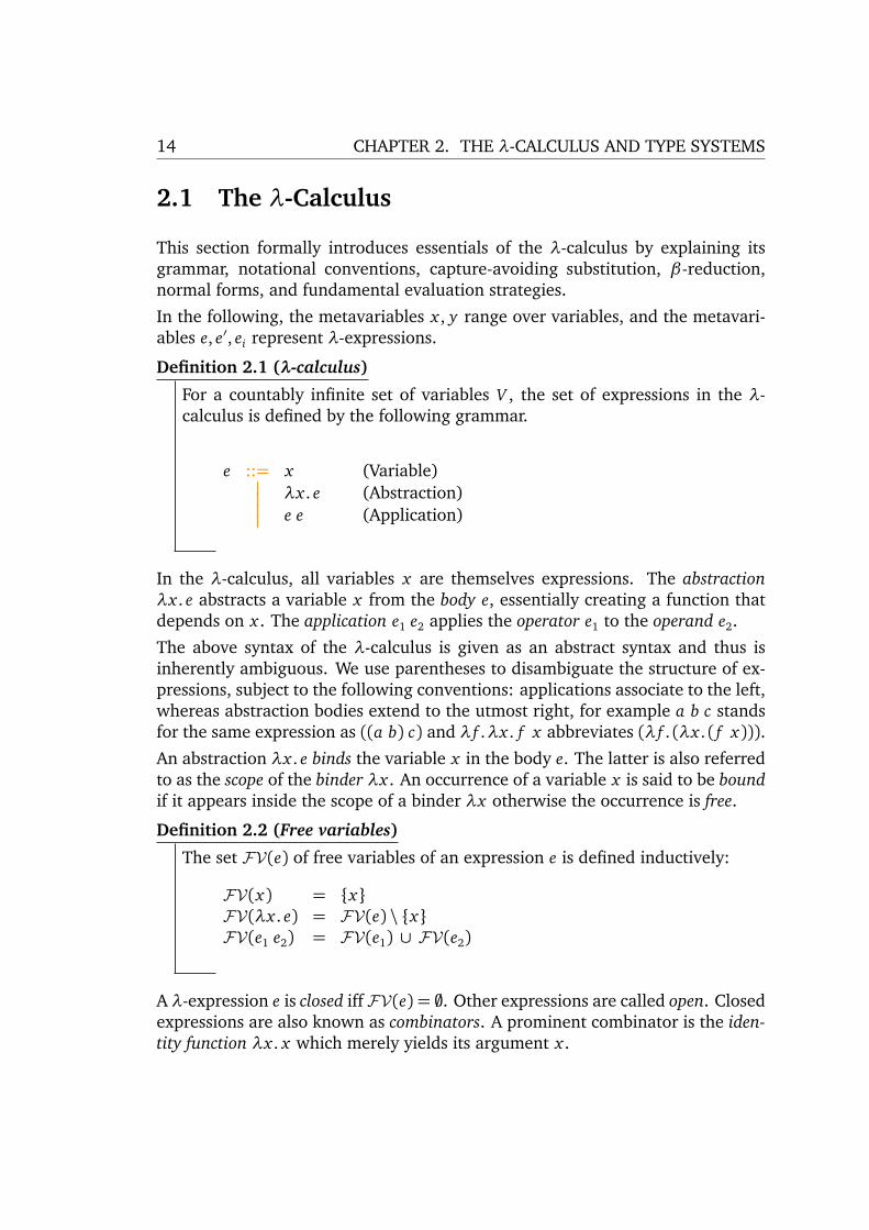
For a countably infinite set of variables V , the set of expressions in the λ-calculus is defined by the following grammar.
e ::= x (Variable)�
� λx . e (Abstraction)�
� e e (Application)
In the λ-calculus, all variables x are themselves expressions. The abstractionλx . e abstracts a variable x from the body e, essentially creating a function thatdepends on x . The application e1 e2 applies the operator e1 to the operand e2.
The above syntax of the λ-calculus is given as an abstract syntax and thus isinherently ambiguous. We use parentheses to disambiguate the structure of ex-pressions, subject to the following conventions: applications associate to the left,whereas abstraction bodies extend to the utmost right, for example a b c standsfor the same expression as ((a b) c) and λ f .λx . f x abbreviates (λ f . (λx . ( f x))).
An abstraction λx . e binds the variable x in the body e. The latter is also referredto as the scope of the binder λx . An occurrence of a variable x is said to be boundif it appears inside the scope of a binder λx otherwise the occurrence is free.
Definition 2.2 (Free variables)
The set FV(e) of free variables of an expression e is defined inductively:
FV(x) = {x}FV(λx . e) = FV(e) \ {x}FV(e1 e2) = FV(e1) ∪ FV(e2)
A λ-expression e is closed iff FV(e) = ;. Other expressions are called open. Closedexpressions are also known as combinators. A prominent combinator is the iden-tity function λx . x which merely yields its argument x .

2.1. THE λ-CALCULUS 15
Expressions that differ only in the names of bound variables are said to be syntac-tically equivalent or α-equivalent, written e1 ≡ e2. For example, λx . x ≡ λy. y. Wemay freely convert between α-equivalent expressions by consistent renaming ofbound variables. Without loss of generality, we adopt the following convention(also known as the Barendregt convention [5]):
Convention 2.3 (Variable convention)
If e1, ..., en appear in a certain mathematical context (definition, proof), thenin these expressions all bound variables are chosen to be different from thefree variables.
The variable convention allows us to provide a straightforward definition ofcapture-avoiding substitution. The function e[x 7→ e′] replaces all free occur-rences of a variable x in an expression e by an expression e′. For example,(λx . y)[y 7→ z] = λx . z, (λx . x)[y 7→ z] = λx . x , and ( f y)[ f 7→ λx . x] =(λx . x) y.
Definition 2.4 (Substitution)
The substitution function e[x 7→ e′] is defined recursively:
x[x 7→ e′] = e′
y[x 7→ e′] = y if y 6= x(λy. e)[x 7→ e′] = λy. (e[x 7→ e′]) if y 6= x , y /∈ FV(e′)(e1 e2)[x 7→ e′] = (e1[x 7→ e′]) (e2[x 7→ e′])
The variable convention ensures that the condition in the third clause alwaysholds so that no further clauses are required.Evaluation of λ-expressions is performed via β-reduction which captures the ideaof function application. The application of abstractions to operands is explainedin terms of substitution.Definition 2.5 (Redex, β-reduction)
An application of the form (λx . e1) e2 is called a reducible expression, β-redex,or simply redex. The β-reduction rule replaces a redex (λx . e1) e2 by the ab-straction body e1 in which all free occurrences of x are substituted with theoperand e2.
(λx . e1) e2→β e1[x 7→ e2]
Given two λ-expressions e and e′, we say that e is β-reducible to e′, writtene →∗β e′, iff there exists a finite, potentially empty sequence of β-reductions

16 CHAPTER 2. THE λ-CALCULUS AND TYPE SYSTEMS
e →β ...→β e′ that transforms e into e′. The evaluation of a λ-expression stopsonce no further redices remain in an expression. From an operational point ofview, such a normal form may be regarded as a computational result.Definition 2.6 (Normal form)
A λ-expression is said to be in normal form if it cannot be reduced any further.A λ-expression e is said to have a normal form if e →∗β e′ holds for some λ-expression e′ in normal form.
Not every λ-expression has a normal form. A simple counterexample of this isthe divergent combinator ω whose evaluation incessantly yields itself.
ω≡ (λx . x x) (λx . x x)→β (λx . x x) (λx . x x)≡ω.
Typically, an expression under evaluation contains more then one redex to choosefrom for the next evaluation step. This gives rise to evaluation strategies that re-duce the individual redices of a λ-expression in a deterministic order. A choicefor a particular strategy has significant impact on both the semantics and theimplementation of a programming language.
• Under normal order reduction (leftmost-outermost), the leftmost redex ofan expression that is not contained in any other redex is reduced first.This means that operations are applied to unevaluated operands therebydeferring the operands’ evaluation.
• Under applicative order reduction (leftmost-innermost), the leftmost redexof an expression that does not contain any further redices is reduced first.Therefore, both the operator and the operand of an application are reducedbefore the application itself.
Normal order evaluation has the advantage that it will reach the normal formof an expression if one exists. As a downside, normal-order evaluation can en-tail significant overhead as redices in the unevaluated operand may be copied,thereby duplicating computations.Applicative order will not normalise an expression if the evaluation of the operanddoes not terminate (for example (λx . e) ω). However, if the evaluation of theoperand terminates, the result will only be computed once and can potentiallybe used many times in the body of the abstraction.Functional programming languages such as SML [75, 70, 49], OCAML [69, 22],HASKELL [81, 13, 54], and CLEAN [84] employ strategies that, unlike the strate-gies presented so far, do not evaluate expressions inside of abstractions. Insteadof transforming expressions into full normal forms, these strategies merely com-pute weak normal forms [91, 80].

2.2. AN APPLIED λ-CALCULUS 17
Definition 2.7 (Weak normal form)
A λ-expression is said to be in weak normal form iff it is an abstraction thatmay contain redices in its body.
Restricting the above evaluation strategies to weak normal forms gives rise tothe two predominant evaluation strategies used by language implementations.
• The call-by-name strategy restricts normal order reduction. The opera-tor is reduced to weak normal form and then applied to the unevaluatedoperand. To avoid multiple evaluation of the operand, concrete implemen-tations such as HASKELL and CLEAN refine this strategy even further to avariant called call-by-need or lazy evaluation. Instead of copying the uneval-uated argument to all variable locations in the syntax tree, only a pointer toa common thunk containing the argument is propagated. Upon first evalu-ation of the argument, the thunk is updated to hold the appropriate valuefor future access.
• Similarly, the call-by-value regime restricts applicative order reduction suchthat both the operator and the operand are merely reduced to weak nor-mal forms before β-reduction is performed. Call-by-value is fairly easy toimplement in an efficient way and therefore is the most widely used eval-uation strategy. For example, SML and OCAML implement call-by-valueevaluation.
2.2 An Applied λ-Calculus
This section presents an applied λ-calculus that extends the bare λ-calculus withthe usual representations of truth values and integers along with primitive op-erators. We define δ-reduction, values, the evaluation relation, and formallydiscuss essential properties of the latter.Definition 2.8 (δ-redex, δ-reduction)
An application of a primitive operator to legitimate arguments is called aδ-redex. δ-reduction, written e ⇒δ e, replaces the redex by the result.
Legitimate arguments are those, on which the operator is defined. For example,* 6 7 ⇒δ 42. For the sake of readability, applications of binary operations mayalso be written in infix notation with the usual precedence rules.Figure 2.1 defines the syntax and the operational semantics of an applied λ-calculus with a call-by-value semantics that may be regarded as a simple pro-gramming language. The top half defines a set of expressions, a set of constant

18 CHAPTER 2. THE λ-CALCULUS AND TYPE SYSTEMS
Syntax
e ::= x�
� λx . e�
� e e�
� c�
� if e then e else e Expressionsc ::= B
�
� Z�
� f 1�
� f 2 Constantsf 1 ::= not Unopsf 2 ::= ↔
�
� &�
� |�
� =�
� <�
� +�
� -�
� * Binops
v ::= λx . e�
� c�
� f 2 v Values
Evaluation e ⇒ e
e1 ⇒ e′1 (E-APP1)e1 e2 ⇒ e′1 e2
e2 ⇒ e′2 (E-APP2)v1 e2 ⇒ v1 e′2
(λx . e1) v2 ⇒ e1[x 7→ v2] (E-ABSAPP)
f 1(v) ⇒δ v′(E-PRFAPP1)
f 1 v ⇒ v′f 2(v1, v2) ⇒δ v3 (E-PRFAPP2)( f 2 v1) v2 ⇒ v3
ep ⇒ e′p(E-COND)
if ep then et else ee ⇒ if e′p then et else ee
if true then et else ee ⇒ et (E-THEN)
if false then et else ee ⇒ ee (E-ELSE)
Figure 2.1: An applied λ-calculus with call-by-value evaluation
symbols and a set of values. In the remainder, the metavariables v, v′, vi rangeover values, the metavariable c represents constant symbols, and a metavariablef n represents function symbols of arity n.
The set of expressions consists of the expressions of the λ-calculus, constantsymbols c and the conditional expression if ep then et else ee, with the predicateep and the two branch expressions et , ee. The set of constant symbols comprisesthe truth values B = {true,false}, the integers Z = {..,−1,0, 1, ..}, and someof the usual logical, relational, and arithmetic operators. A value is either a λ-abstraction, a constant symbol c, or an application f 2 v of a binary operator to asingle argument.
Definition 2.9 (Value)
A value v is an expression that is considered a valid evaluation result.

2.2. AN APPLIED λ-CALCULUS 19
The bottom half of Figure 2.1 defines the operational semantics of the languageby means of inference rules.
Definition 2.10 (One-step evaluation relation, multi-step evaluation relation)
The one-step evaluation relation e ⇒ e is the smallest relation that satisfiesthe inference rules. The multi-step evaluation relation e ⇒∗ e is the reflexive,transitive closure of e ⇒ e.
The evaluation relation captures the call-by-value strategy: the rules E-APP1and E-APP2 process applications from left to right and bottom-up; when theoperator is an abstraction and the operand is a value, E-ABSAPP performs a β-reduction step. The definition of the capture-avoiding substitution carries overfrom Section 2.1, mutatis mutandis. The rules E-APPPRF1 and E-APPPRF2 eval-uate applications of primitive functions to legitimate arguments by means ofδ-reduction. Evaluation of the conditional is defined by the final three rules.E-COND evaluates the predicate. When it evaluates to either true or false, theentire conditional is evaluated to et (E-THEN) or ee (E-ELSE), respectively. Noevaluation takes place inside of abstractions.Every expression in normal form that is not a value is said to be a stuck expres-sion [82]. For example, not 42, (λx . x) + 0, if 42 then true else false. Theintuition behind stuck expressions is that due to a run-time error, the machinehas entered a meaningless state in which no further evaluation is possible.We can now formally discuss essential properties of the evaluation relation. First,we check that every value is in normal form, a crucial property of every languagedefinition.Theorem 2.11
Every value v is in normal form.
Proof : Immediate. There are no rules that evaluate abstractions λx . e, constant symbolsc, or partially applied binary operators f 2 v.
The next theorem states that one-step evaluation is deterministic, i. e., the resultof an expression that makes an evaluation step will always be the same.
Theorem 2.12 (Determinacy of one-step evaluation)
If e ⇒ e′ and e ⇒ e′′, then e = e′′.
Proof : By induction on a derivation of e ⇒ e′. For every rule E, we assume that eevaluates to e′. We show that no other rule that matches e than E is applicable. Inconsequence, e′′ can only be derived from e by rule E. By the induction hypothesis,evaluation of the subexpressions is deterministic and hence e′ = e′′.

20 CHAPTER 2. THE λ-CALCULUS AND TYPE SYSTEMS
1. Case E-APP1: e = e1 e2 with e1 ⇒ e′1. Since e1 is not a value, no other rule matchese. By the hypothesis e′1 = e′′1 and hence e′ = e′′.
2. Case E-APP2: e = v1 e2 with e2 ⇒ e′2. Similar.
3. Case E-ABSAPP: e = (λx . e1) v2. Both the operator and the operand are values, sono other rule matches e. Substitution is deterministic, so that e′ = e′′.
4. Case E-PRFAPP1: e = f 1 v with f 1(v) ⇒δ v′. No other rule matches and δ-reduction is deterministic, so that e′ = e′′
5. Case E-PRFAPP2: e = ( f 2 v1) v2 with f 2(v1, v2) ⇒δ v3. Similar.
6. Case E-COND: e = if ep then et else ee with ep ⇒ e′p. Since ep is not a value, noother rule matches e. By the hypothesis, e′p = e′′p and thus e′ = e′′.
7. Case E-THEN: e = if true then et else ee. No other rule matches e and thereforee′ = e′′.
8. Case E-FALSE: e = if false then et else ee. Similar.
An immediate corollary of the determinacy of one-step evaluation is that multi-step evaluation is also deterministic.Corollary 2.13 (Uniqueness of normal forms)
If e ⇒∗ e′ and e ⇒∗ e′′ where e′ and e′′ are normal forms, then e′ = e′′.
In addition to the facilities for function definition and application, an appliedλ-calculus features built-in constant symbols and operators whose operationalsemantics is defined in terms of δ-reduction. This section introduced an appliedλ-calculus with a call-by-value evaluation regime that serves as a language nu-cleus in the remainder of the thesis. We showed that evaluation is deterministicand that every value is in normal form. All language extensions must retain theseessential properties.
2.3 Simple Types
Every terminating evaluation sequence either yields a value or ends at a stuckexpression, i. e., an expression for which no evaluation rule applies although it isnot considered a valid result. A type system identifies such errors by classifyingexpressions according to the values they evaluate to. This section augments theapplied λ-calculus from the previous section with simple types. We define thetyping relation and discuss essential properties of the typed calculus, such astype safety.Figure 2.2 shows a typed version of the applied λ-calculus from Section 2.2 byproviding a syntax, an evaluation relation, and a typing relation.

2.3. SIMPLE TYPES 21
Syntax
T ::= B�
� T → T TypesB ::= bool
�
� int Base types
e ::= x�
� λx : T . e�
� e e�
� c�
� if e then e else e Expressionsc ::= B
�
� Z�
� f 1�
� f 2 Constantsf 1 ::= not Unopsf 2 ::= ↔
�
� &�
� |�
� =�
� <�
� +�
� -�
� * Binops
v ::= λx : T . e�
� c�
� f 2 v Values
Γ ::= ·�
� Γ, x : T Context
Evaluation e ⇒ ee1 ⇒ e′1 (E-APP1)
e1 e2 ⇒ e′1 e2
e2 ⇒ e′2 (E-APP2)v1 e2 ⇒ v1 e′2
(λx : T . e1) v2 ⇒ e1[x 7→ v2] (E-ABSAPP)
f 1(v) ⇒δ v′(E-PRFAPP1)
f 1 v ⇒ v′f 2(v1, v2) ⇒δ v3 (E-PRFAPP2)( f 2 v1) v2 ⇒ v3
ep ⇒ e′p(E-COND)
if ep then et else ee ⇒ if e′p then et else ee
if true then et else ee ⇒ et (E-THEN)
if false then et else ee ⇒ ee (E-ELSE)
Typing Γ ` e : Tx : T ∈ Γ (T-VAR)Γ ` x : T
Γ ` c : type(c) (T-CONST)
Γ, x : T1 ` e : T2 (T-ABS)Γ ` λx : T1. e : T1→ T2
Γ ` e1 : T11→ T12 Γ ` e2 : T11 (T-APP)Γ ` e1 e2 : T12
Γ ` ep : bool Γ ` et : T Γ ` ee : T(T-COND)
Γ ` if ep then et else ee : T
Figure 2.2: The applied λ-calculus with simple types
22 CHAPTER 2. THE λ-CALCULUS AND TYPE SYSTEMS
In addition to expressions, constants, and values, the syntax defines a set of typesand a set of typing contexts. In the following, the metavariables T, T ′, Ti rangeover types and the metavariables Γ,Γ′,Γi range over contexts.The set of types consists of the base types bool and int, that describe booleanand integer expressions, and function types T1→ T2 that describe functions withthe domain T1 and codomain T2. The function type associates to the right, so thatT1 → T2 → T3 stands for T1 → (T2 → T3). The expressions and values resemblethose from Section 2.2, except that abstractions λx : T . e are annotated with thetype of the bound variable.A type context or environment is a sequence ·, x1 : T1, ..., xn : Tn that, starting withthe empty context ·, associates variables with types. Convention 2.3 extends tothe variables bound in a context, so that a variable can appear in a context Γat most once. The function dom(Γ) yields the set of variables bound in Γ. Thenotation x : T ∈ Γ means that in Γ, the variable x is associated with type T .The evaluation relation e ⇒ e is, apart from the rule E-ABSAPP the same as inSection 2.2. The bottom of the figure defines the ternary typing relation Γ ` e : Tby a set of inference rules.Definition 2.14 (Typing relation, well-typed expression)
The typing relation Γ ` e : T is the smallest ternary relation between typingcontexts, expressions, and types that satisfies the inference rules. An expres-sion e is said to be well-typed under a context Γ iff there is some T such thatΓ ` e : T .
The typing rule T-VAR assigns a variable x the type T if x : T appears in thecontext Γ. The rule T-CONST gives types to constants c according to the tableshown in Figure 2.3. The typing rule T-ABS for abstractions assign the abstrac-tion λx : T . e the type T → T ′ when e has type T ′ under the extended contextΓ, x : T . Applications e1 e2 are checked by the rule T-APP. When the operator e1
is a function of type T → T ′ and when the operand e2 is an argument of typeT , then the application result has type T ′. Finally, the typing rule T-COND forconditionals if ep then et else ee ensures that the predicate ep is a booleanexpression and that the branch expressions et , ee have the same type T .The goal of type checking is to rule out programs whose evaluation might getstuck at some point. This property is called safety or soundness. To formallyprove that simple types indeed provide type-safety, two theorems are required.The progress theorem states that every (closed) well-typed expression is either avalue or able to make an evaluation step. The preservation theorem (or subjectreduction) states that evaluation preserves the type of an expression such thatthe progress theorem applies again.A basic assumption about the constant and function symbols in the calculus is

2.3. SIMPLE TYPES 23
true,false : bool
not : bool→ bool
↔,&,| : bool→ bool→ bool
..,-1,0,1, .. : int
=,< : int→ int→ bool
+,-,* : int→ int→ int
Figure 2.3: Types of the constant symbols
that every symbol has a type and that δ-reduction of a function symbol behavesas declared by its type.
Axiom 2.15 (Constant symbols are well-behaved)
Each constant symbol c has a type type(c) such that: if type( f 1) = T1 → T2,then δ-reduction f 1(v1) ⇒δ v2 is defined for all values v1 with · ` v1 : T1
so that · ` v2 : T2. The axiom also applies to binary functions f 2, mutatismutandis.
The canonical forms lemma recapitulates the possible forms the values of a giventype may have. The proof is omitted as it is straightforward from the syntax ofvalues, the types of constants, and the typing rules.
Lemma 2.16 (Canonical forms)
1. If v is a value with · ` v : bool then v ∈ B.
2. If v is a value with · ` v : int then v ∈ Z.
3. If v is a value with · ` v : T1 → T2 then v = f 1, v = f 2, v = f 2 v1, orv = λx : T . e.
With the canonical forms lemma, the progress theorem can be formalised andproved.
Theorem 2.17 (Progress)
If · ` e : T then e is a value or there is some e′ with e ⇒ e′.
Proof : By induction on type derivations · ` e : T .
1. Case T-VAR: e = xe is not closed.
2. Case T-CONST: e = ce is a value.

24 CHAPTER 2. THE λ-CALCULUS AND TYPE SYSTEMS
3. Case T-ABS: e = λx : T . ee is a value.
4. Case T-APP: e = e1 e2 with · ` e1 : T ′→ T and · ` e2 : T ′
By the hypothesis, the subexpressions e1 and e2 are either values or can make anevaluation step. If e1 can make a step, E-APP1 applies. If e1 is a value and e2 canmake a step then E-APP2 applies. If both expressions are values, the applicationcan have four different forms according to the canonical forms lemma:
(a) Case e1 = f 1: E-PRFAPP1 applies because of axiom 2.15.(b) Case e1 = f 2: e = f 2 e2 is a value.(c) Case e1 = f 2 v1: E-PRFAPP2 applies because of axiom 2.15.(d) Case e1 = λx : T ′. e′: E-ABSAPP applies.
5. Case T-COND: e = if ep then et else ee with · ` ep : boolBy the hypothesis, ep is a value or it can make an evaluation step. If e1 can make astep, then E-COND applies. If e1 is a value, then by the canonical forms lemma, itis either true or false and therefore either E-THEN or E-ELSE applies.
In order to prove preservation, some basic lemmas are required. The weakeninglemma states that extending a context with a fresh variable x does not changethe type of a well-typed expression. The proof is a straightforward induction ontyping derivations Γ1,Γ2 ` e : T .Lemma 2.18 (Weakening)
If Γ1,Γ2 ` e : T then Γ1, x : Tx ,Γ2 ` e : T .
The substitution lemma states that substituting an identifier x of type Tx with anexpression ex of the same type Tx in an expression e preserves the type of e.Lemma 2.19 (Substitution lemma)
If Γ1, x : Tx ,Γ2 ` e : T and Γ1 ` ex : Tx then Γ1,Γ2 ` e[x 7→ ex] : T .
Proof : By induction on the derivation of Γ1, x : Tx ,Γ2 ` e : T .
1. Case T-CONST: Γ1, x : Tx ,Γ2 ` c : type(c), c[x 7→ ex] = cBy T-CONST, Γ1,Γ2 ` c : type(c).
2. Case T-VAR: Γ1, x : Tx ,Γ2 ` x ′ : T , x ′ : T ∈ (Γ1, x : Tx ,Γ2).
(a) Case x ′ = x: x ′[x 7→ ex] = exSince Tx = T , Γ1 ` ex : T . By weakening, Γ1,Γ2 ` ex : T .
(b) Case x 6= x ′: x ′[x 7→ ex] = x ′
Since x 6= x ′, x ′ : T ∈ (Γ1,Γ2). By T-VAR, Γ1,Γ2 ` x ′ : T .
3. Case T-ABS: Γ1, x : Tx ,Γ2 ` λx ′ : T1. e : T1→ T2, Γ1, x : Tx ,Γ2, x ′ : T1 ` e : T2.By the variable convention 2.3, x 6= x ′ and x ′ 6∈ FV(ex). By the hypothesis,Γ1,Γ2, x ′ : T1 ` e[x 7→ ex] : T2. By T-ABS, Γ1,Γ2 ` λx ′ : T1. e[x 7→ ex] : T1→ T2.
2.3. SIMPLE TYPES 25
4. Case T-APP: e = e1 e2: By the induction hypothesis and T-APP.
5. Case T-COND: e = if ep then et else ee: By the induction hypothesis and T-COND.
The evaluation of β-redices involves substituting identifiers with expressions.The proof of the preservation theorem thus relies on the substitution lemma.
Theorem 2.20 (Preservation)
If Γ ` e : T and e ⇒ e′ then Γ ` e′ : T .
Proof : By induction on type derivations Γ ` e : T .
1. Case T-VAR: e = xThere is no e′ with x ⇒ e′.
2. Case T-CONST: e = ce is a value.
3. Case T-ABS: e = λx : T ′. ee is a value.
4. Case T-APP: e = e1 e2 with Γ ` e1 : T ′→ T and Γ ` e2 : T ′
The application can make an evaluation step in five possible ways:
(a) Case E-APP1: e1 ⇒ e′1 then e′ = e′1 e2The result follows from the induction hypothesis and T-APP.
(b) Case E-APP2: e1 = v1 and e2 ⇒ e′2 then e′ = v1 e′2Similar.
(c) Case E-APPAPS: e1 = λx : T ′. eb and e2 = v2 then e′ = eb[x 7→ v2]By the substitution lemma, Γ ` eb[x 7→ v2] : T .
(d) Case E-PRFAPP1: e1 = f 1 and e2 = v2 with f 1(v2) ⇒δ v then e′ = vBy axiom 2.15, δ-reduction is type-preserving.
(e) Case E-PRFAPP2: e1 = f 2 v1 and e2 = v2 with f 2(v1, v2) ⇒δ v then e′ = vSimilar.
5. Case T-COND: e = if ep then et else ee with Γ ` ep : bool, Γ ` et : T , Γ ` ee : TThe conditional can make an evaluation step in three possible ways:
• Case E-COND: ep ⇒ e′p then e′ = if e′p then et else eeBy the hypothesis and T-COND.
• Case E-THEN: ep = true then e′ = etImmediate, since Γ ` et : T .
• Case E-ELSE: ep = false then e′ = eeSimilar.
Unlike the untyped λ-calculus, the simply-typed λ-calculus is strongly normal-ising, i. e., the evaluation of every well-typed expression eventually terminates

26 CHAPTER 2. THE λ-CALCULUS AND TYPE SYSTEMS
yielding a value. For example, there is no typed form of the divergent combina-tor ω= (λx . x x) (λx . x x) as the inherent self-application x x cannot be typed.Lemma 2.21 (Self-application is ill-typed)
There is no context Γ and no type T so that Γ ` x x : T .
Proof : By reductio ad absurdum. Suppose that under some context Γ, there is sometype T so that Γ ` x x : T . By inversion of the typing rule T-APP, there must be some T ′
with Γ ` x : T ′→ T and simultaneously Γ ` x : T ′. Therefore the proposition is wrong.
To nonetheless enable the specification of recursive programs, typed λ-calculi arecommonly extended with some kind of fixed-point expression that reproducesitself upon evaluation.
Summary
This chapter presented essential concepts of the λ-calculus, operational seman-tics, and type systems. By restricting the set of allowed expressions, types enablea compiler to statically rule out erroneous programs. Type checking is inherentlyconservative: only programs for which the absence of certain behaviours can beproved are accepted. As a downside, a type system may also reject well-behavedprograms as ill-typed. To increase the number of typeable programs, more ad-vanced typing schemes have been studied.In the simply-typed λ-calculus, an abstraction λx : T . e may be regarded as anexpression that is parameterised by another expression of type T . Figure 2.4shows Barendregt’s λ-cube [6, 82] that nicely visualises three orthogonal exten-sions of this basic system. The cube places the simply typed λ-calculus in thelower left front corner as λ→. Each of its three axes represents a new form ofabstraction.
1. The vertical axis introduces type abstractions that map types to expressionsand thereby give rise to polymorphism. The resulting calculus is known asSystem F or the second-order λ-calculus.
2. The perpendicular axis introduces type operators, i. e., types that dependon types. The system λω is thus called the simply-typed λ-calculus withtype operators. The combination with System F is known as System Fω.
3. The horizontal axis introduces dependent types, i. e., types that dependon expressions. The λ-calculus with dependent types has become widelyknown as the logical framework LF. The calculus of constructions (CC)combines all three forms of abstraction.

2.3. SIMPLE TYPES 27
λ→
λω
F
Fω
LF
·
·
CC
Figure 2.4: Barendregt’s λ-cube [6, 82]

28 CHAPTER 2. THE λ-CALCULUS AND TYPE SYSTEMS

3Decidable First-Order Theories
The type system of QUBE uses dependent types to accurately model array shapesand to restrict the potential run-time values of expressions. Type checking pro-ceeds in collaboration with an automatic theorem prover for the SatisfiabilityModulo Theories problem. This chapter gives a brief introduction to proposi-tional logic, first-order logic, and the relevant fragments of first-order theoriesthat will be used in later chapters. More detailed presentations of these top-ics can be found in textbooks on logic and computer aided verification, suchas [66, 17, 50].
The remainder of this chapter is structured as follows: First, Section 3.1 intro-duces propositional logic and basic terminology. Section 3.2 then gives a briefaccount of first-order logic, which extends propositional logic with non-logicalfunction symbols, predicate symbols and quantifiers. Next, Section 3.3 presentssome decidable quantifier-free fragments of first-order theories that the QUBE
compiler uses to reason about programs, namely the theory of uninterpretedfunctions and equality as well as linear integer arithmetic. Section 3.4 presentsarray properties, a decidable fragment of quantified first-order logic that is usedby the QUBE compiler to model integer vectors.
29
30 CHAPTER 3. DECIDABLE FIRST-ORDER THEORIES
3.1 Propositional Logic
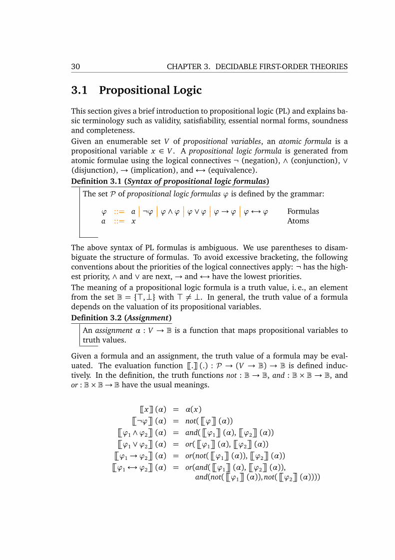
This section gives a brief introduction to propositional logic (PL) and explains ba-sic terminology such as validity, satisfiability, essential normal forms, soundnessand completeness.Given an enumerable set V of propositional variables, an atomic formula is apropositional variable x ∈ V . A propositional logic formula is generated fromatomic formulae using the logical connectives ¬ (negation), ∧ (conjunction), ∨(disjunction),→ (implication), and↔ (equivalence).Definition 3.1 (Syntax of propositional logic formulas)
The set P of propositional logic formulas ϕ is defined by the grammar:
ϕ ::= a�
� ¬ϕ�
� ϕ ∧ϕ�
� ϕ ∨ϕ�
� ϕ→ ϕ�
� ϕ↔ ϕ Formulasa ::= x Atoms
The above syntax of PL formulas is ambiguous. We use parentheses to disam-biguate the structure of formulas. To avoid excessive bracketing, the followingconventions about the priorities of the logical connectives apply: ¬ has the high-est priority, ∧ and ∨ are next,→ and↔ have the lowest priorities.The meaning of a propositional logic formula is a truth value, i. e., an elementfrom the set B = {>,⊥} with > 6= ⊥. In general, the truth value of a formuladepends on the valuation of its propositional variables.Definition 3.2 (Assignment)
An assignment α : V → B is a function that maps propositional variables totruth values.
Given a formula and an assignment, the truth value of a formula may be eval-uated. The evaluation function ¹.º (.) : P → (V → B) → B is defined induc-tively. In the definition, the truth functions not : B → B, and : B× B → B, andor : B×B→ B have the usual meanings.
¹xº (α) = α(x)�
¬ϕ�
(α) = not(�
ϕ�
(α))�
ϕ1 ∧ϕ2
�
(α) = and(�
ϕ1
�
(α),�
ϕ2
�
(α))�
ϕ1 ∨ϕ2
�
(α) = or(�
ϕ1
�
(α),�
ϕ2
�
(α))�
ϕ1→ ϕ2
�
(α) = or(not(�
ϕ1
�
(α)),�
ϕ2
�
(α))�
ϕ1↔ ϕ2
�
(α) = or(and(�
ϕ1
�
(α),�
ϕ2
�
(α)),and(not(
�
ϕ1
�
(α)), not(�
ϕ2
�
(α))))

3.1. PROPOSITIONAL LOGIC 31
Given an assignment α, a formula ϕ is said to hold under α, written α |= ϕ, iff�
ϕ�
(α) =>.Definition 3.3 (Validity, satisfiability)
A formula ϕ is called valid, written |= ϕ, iff ϕ holds under all assignments,otherwise ϕ is called invalid. A formula ϕ is called satisfiable iff ϕ holdsunder some assignment α, otherwise ϕ is called unsatisfiable.
Satisfiability and validity are dual concepts. A formula is valid iff its negationis unsatisfiable. Vice versa, a formula is invalid iff its negation is satisfiable. Asatisfying assignment of a formula ϕ is also called a model of ϕ. An assignmentthat satisfies ¬ϕ is said to be a counterexample of ϕ. Valid formulas are alsocalled tautologies.Definition 3.4 (Equivalence, implication)
Two formulas ϕ1 and ϕ2 are said to be equivalent, written ϕ1 ⇔ ϕ2, if theyevaluate to the same truth values under all assignments. I. e., for all assign-ments α, α |= ϕ1 iff α |= ϕ2, i. e., |= ϕ1↔ ϕ2.The formula ϕ1 is said to imply the formula ϕ2, written ϕ1 ⇒ ϕ2, if everyassignment α satisfying ϕ1 also satisfies ϕ2. I. e., for all assignments α, ifα |= ϕ1, then α |= ϕ2, i. e., |= ϕ1→ ϕ2.
A normal form imposes syntactic restrictions on formulas. The process of decid-ing whether a formula is satisfiable usually starts with transforming the formulato some normal form that is appropriate for the decision procedure at hand.Definition 3.5 (Negation normal form (NNF))
A formula is in negation normal form (NNF) if it is generated from literalsusing the logical connectives ∧ and ∨. A literal is an atom or its negation.
ϕnnf ::= l�
� ϕnnf ∧ϕnnf
�
� ϕnnf ∨ϕnnf NNF formulasl ::= a
�
� ¬a Literals
Every PL formula can be transformed into an equivalent formula in NNF by ex-haustively replacing the left hand sides of the following equivalences with therespective right hand sides.
¬¬ϕ ⇔ ϕ
¬(ϕ1 ∧ϕ2) ⇔ ¬ϕ1 ∨¬ϕ2
¬(ϕ1 ∨ϕ2) ⇔ ¬ϕ1 ∧¬ϕ2
ϕ1→ ϕ2 ⇔ ¬ϕ1 ∨ϕ2
ϕ1↔ ϕ2 ⇔ (ϕ1→ ϕ2)∧ (ϕ2→ ϕ1)

32 CHAPTER 3. DECIDABLE FIRST-ORDER THEORIES
Definition 3.6 (Conjunctive normal form (CNF))
A formula is in conjunctive normal form if it is a conjunction of clauses. Aclause is a disjunction of literals.
ϕcn f ::=∧
i
∨
j li, j CNF formulas
A formula can be transformed into an equivalent formula in CNF by first trans-forming the formula into NNF and then distributing the conjunction symbols byexhaustively applying the following equivalences from left to right.
(ϕ1 ∧ϕ2)∨ϕ3 ⇔ (ϕ1 ∨ϕ3)∧ (ϕ2 ∨ϕ3)ϕ1 ∨ (ϕ2 ∧ϕ3) ⇔ (ϕ1 ∨ϕ2)∧ (ϕ1 ∨ϕ3)
The decision problem is to determine whether a formula is valid. Because of theduality of validity and satisfiability, determining the satisfiability of the negatedformula is an equivalent problem. We are interested in automatic procedures todetermine the validity (or the unsatisfiability) of a given formula.
Definition 3.7 (Decision procedure)
A procedure for the decision problem is sound if when it returns valid (un-satisfiable), the formula is indeed valid (unsatisfiable). A procedure for thedecision problem is complete if it terminates on every input, and when theformula is valid (unsatisfiable), it returns valid (unsatisfiable).A procedure is called a decision procedure if it is sound and complete.
The satisfiability problem of boolean formulas (SAT) is naïvely decidable becausethe number of potential assignments is finite. Given a formula with n proposi-tional variables, a decision procedure may simply enumerate all 2n assignmentsand report whether any of these satisfies the formula.
SAT was the first knownNP-complete problem [27]. It is thus unknown whetherthere is an algorithm that finds a satisfying assignment for all satisfiable for-mulas in polynomial time. Nonetheless, the theoretical and practical signifi-cance of the problem has motivated the development of extremely powerful SATsolvers. Based on the Davis-Putnam-Loveland-Logemann (DPLL) algorithm [29,28], solvers like CHAFF [77] and MINISAT [34] are used in the industrial practiceto solve CNF formulas with hundreds of thousands or even millions of booleanvariables in reasonable amounts of time.

3.2. FIRST-ORDER LOGIC 33
3.2 First-Order Logic
First-order logic (FOL), also called predicate logic, extends propositional logicwith non-logical function and predicate symbols and quantification. Terms eval-uate to objects, predicates take objects to truth values. Quantifiers express prop-erties of entire sets of objects.A signature fixes the set of non-logical symbols that may appear in a first-orderformula.Definition 3.8 (Signature)
A signature Σ = (F,P) consists of a family F= (Fn)n∈N of function symbols, anda family P= (Pn)n∈N of predicate symbols. n is called the arity of a symbol. Weassume all sets to be mutually disjoint.
Nullary function symbols may be regarded as constant symbols. Given a signa-ture Σ = (F,P) and an enumerable set V of variables, a term is either a variablex ∈ V , or an application of a function symbol fn ∈ Fn to n terms. An atomicformula is an application of a predicate symbol pn ∈ Pn to n terms. A first-order formula consists of atomic formulas,combined with the logical connectives¬ (negation), ∧ (conjunction), ∨ (disjunction),→ (implication), and↔ (equiv-alence), and the quantifiers ∀x (for all x) and ∃x (for some x).Definition 3.9 (Syntax of terms and first-order formulas)
The set T of terms t and the set F of first-order formulas ϕ over Σ and V aredefined by the following grammar:
ϕ ::= a�
� ¬ϕ�
� ϕ ∧ϕ�
� ϕ ∨ϕ�
� ϕ→ ϕ�
� ϕ↔ ϕ Formulas�
� ∀x .ϕ�
� ∃x .ϕa ::= pn(t1, ..., tn) Atomst ::= x
�
� fn(t1, ..., tn) Terms
As before, we use parentheses to disambiguate the structure of first-order for-mulas. The following conventions about the order of operations apply: ¬ is eval-uated first, ∧ and ∨ are evaluated next, then quantifiers are evaluated, beforefinally→ and↔ are evaluated.In analogy with the λ-calculus, a variable is called free in a formula ϕ, iff at leastone occurrence is not bound by a quantifier. The set FV(ϕ) contains all freevariables of ϕ. A formula that contains no free variable is called a closed formulaor a sentence.An interpretation gives meaning to a signature. It provides a domain for in-terpreting variables and terms, for example, the integers or real numbers, and
34 CHAPTER 3. DECIDABLE FIRST-ORDER THEORIES
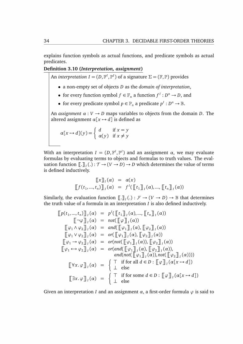
explains function symbols as actual functions, and predicate symbols as actualpredicates.Definition 3.10 (Interpretation, assignment)
An interpretation I = (D,FI ,PI) of a signature Σ = (F,P) provides
• a non-empty set of objects D as the domain of interpretation,
• for every function symbol f ∈ Fn a function f I : Dn→ D, and
• for every predicate symbol p ∈ Pn a predicate pI : Dn→ B.
An assignment α : V → D maps variables to objects from the domain D. Thealtered assignment α[x 7→ d] is defined as
α[x 7→ d](y) =�
d if x = yα(y) if x 6= y
With an interpretation I = (D,FI ,PI) and an assignment α, we may evaluateformulas by evaluating terms to objects and formulas to truth values. The eval-uation function ¹.ºI (.) : T → (V → D)→ D which determines the value of termsis defined inductively.
¹xºI (α) = α(x)�
f (t1, ..., tn)�
I (α) = f I(�
t1
�
I (α), ...,�
tn�
I (α))
Similarly, the evaluation function ¹.ºI (.) : F → (V → D) → B that determinesthe truth value of a formula in an interpretation I is also defined inductively.
�
p(t1, ..., tn)�
I (α) = pI(�
t1
�
I (α), ...,�
tn�
I (α))�
¬ϕ�
I (α) = not(�
ϕ�
I (α))�
ϕ1 ∧ϕ2
�
I (α) = and(�
ϕ1
�
I (α),�
ϕ2
�
I (α))�
ϕ1 ∨ϕ2
�
I (α) = or(�
ϕ1
�
I (α),�
ϕ2
�
I (α))�
ϕ1→ ϕ2
�
I (α) = or(not(�
ϕ1
�
I (α)),�
ϕ2
�
I (α))�
ϕ1↔ ϕ2
�
I (α) = or(and(�
ϕ1
�
I (α),�
ϕ2
�
I (α)),and(not(
�
ϕ1
�
I (α)), not(�
ϕ2
�
I (α))))�
∀x .ϕ�
I (α) =�
> if for all d ∈ D :�
ϕ�
I (α[x 7→ d])⊥ else
�
∃x .ϕ�
I (α) =�
> if for some d ∈ D :�
ϕ�
I (α[x 7→ d])⊥ else
Given an interpretation I and an assignment α, a first-order formula ϕ is said to

3.2. FIRST-ORDER LOGIC 35
hold in I under α, written α |=I ϕ, iff�
ϕ�
I (α) = >. A formula ϕ is said to holdin I , written |=I ϕ, iff ϕ holds in I under any assignment.
Definition 3.11 (Validity, satisfiability)
A first-order sentence ϕ is valid, written |= ϕ, iff ϕ holds in all interpretations,otherwise ϕ is invalid. The sentence ϕ is satisfiable, iff ϕ holds in someinterpretation, otherwise ϕ is unsatisfiable.
Validity and satisfiability are only defined for closed formulas. By convention,we say that a (non-closed) formula ϕ is valid, iff its universal closure ∀ ∗ .ϕ isvalid. Dually, we call ϕ satisfiable, iff its existential closure ∃ ∗ .ϕ is satisfiable.The normal forms of propositional logic have counterparts in first-order logic.We restrict the presentation to the first-order extension of negation normal formas we will use it later in Section 3.4.Definition 3.12 (Negation normal form (NNF))
A first order formula is in negation normal form (NNF) if it contains only ¬,∧, and ∨ as logical connectives and negation appears only in literals. A literalis an atom or its negation.
ϕnnf ::= l�
� ϕnnf ∧ϕnnf
�
� ϕnnf ∨ϕnnf NNF formulas�
� ∀x .ϕnnf
�
� ∃x .ϕnnf
l ::= a�
� ¬a Literals
In order to transform a first-order formula to an equivalent formula in negationnormal form, the equivalences for normalising propositional logic formulas fromSection 3.1 may be applied from left to right. Additionally, the following twoequivalences push down negation symbols into quantified formulas.
¬∀x .ϕ ⇔ ∃x .¬ϕ¬∃x .ϕ ⇔ ∀x .¬ϕ
The function and predicate symbols of a signature are purely syntactic. Theirmeanings are subject to interpretation. Coincidentally, we may decide to in-terpret the function symbol + ∈ F2 as integer addition, but entirely differentinterpretations are possible, too. A first-order theory restricts the interpretationof non-logical symbols by specifying additional axioms.
Definition 3.13 (First-order theory)
A theory T = (Σ,A) is defined by a signature Σ and a set A of axioms thatprovide meaning to the non-logical symbols of Σ. Each axiom is a Σ-sentence.
36 CHAPTER 3. DECIDABLE FIRST-ORDER THEORIES
The concepts of validity and satisfiability can be refined to take theory-specificaxioms into account.Definition 3.14 (T -validity, T -satisfiability)
For a given theory T = (Σ,A), a Σ-sentence ϕ is said to be T -valid iff allinterpretations that satisfy the axioms in A also satisfy ϕ. The sentence ϕ iscalled T -satisfiable, iff there is an interpretation that satisfies both the axiomsof T and ϕ.
A theory restricts the interpretation of the non-logical symbols in formulas. Incontrast, restricting the syntax of a logic language yields a fragment of that logic.For example, the quantifier-free fragment of a theory T is the set of all T -validformulas without quantifiers.
3.3 Quantifier-Free Fragments ofFirst-Order Theories
This section briefly describes the quantifier-free fragments of first-order theoriesthat the QUBE compiler uses to reason about expressions. Specifically, these arethe theory of equality and uninterpreted functions, and linear integer arithmetic.A simple but useful first-order theory is the theory of equality in conjunction withuninterpreted functions (and predicates).
Definition 3.15 (Equality with uninterpreted functions)
The theory of equality with uninterpreted functions TEU F extends an arbitrarysignature Σ = (F,P) with a single interpreted equality predicate =∈ P2.
The axioms of equality logic ensure that = denotes an equivalence relation byprescribing that = should be reflexive, symmetric, and transitive.
1. ∀x . x = x (Reflexivity)
2. ∀x , y. x = y↔ y = x (Symmetry)
3. ∀x , y, z. x = y ∧ y = z→ x = z (Transitivity)
Furthermore, all interpretations of function and predicate symbols should be-have consistent: functions and predicates must always evaluate to equal valueswhen given equal arguments. Apart from functional consistency, symbols areuninterpreted.The following axioms ensure that term and predicate construction is compatiblewith equality, such that it becomes a congruence relation.

3.3. QUANTIFIER-FREE FRAGMENTS OF FIRST-ORDER THEORIES 37
4. for all function symbols f ∈ Fn
∀xn, yn.�∧
i x i = yi
�
→ ( f (xn) = f (yn)) (Function congruence)
5. for all predicate symbols p ∈ Pn
∀xn, yn.�∧
i x i = yi
�
→ (p(xn)↔ p(yn)) (Predicate congruence)
Satisfiability checking in the quantifier-free fragment of TEU F is decidable. Incomputer aided verification, uninterpreted functions are widely used as substi-tutes for functions whose exact semantics is either too complex for mechanicalproof or even entirely irrelevant for proving the formula at hand.
Example 3.16 (Equality checking with uninterpreted functions)
Functional consistency is sufficient to prove the equality of the expressions1. let x = a ∗ b in let y = x ∗ c in y, and
2. (a ∗ b) ∗ c.Rewrite in TEU F , and prove the validity of
x = fmul(a, b)∧ y = fmul(x , c)→ y = fmul( fmul(a, b), c) ,
or equivalently, prove the unsatisfiability of
x = fmul(a, b)∧ y = fmul(x , c)∧ y 6= fmul( fmul(a, b), c) .
Merely relying on functional consistency is insufficient to prove all correct state-ments. Thus, validity checking of an arbitrary formula by approximating it inTEU F is sound but not complete. For example, equalities arising from the com-mutativity of addition such as a+ b = b+ a cannot be proved in TEU F . However,in the context of array programming, where ranks, shapes, and array indices areall (vectors of) integers, it is particularly important to accurately reason about(in-)equalities of integers. The theory of linear integer arithmetic allows us toexpress and reason about such constraints.
Definition 3.17 (Linear integer arithmetic)
The signature of the theory of linear integer arithmetic provides an infiniteset F0 = Z of constant symbols, an infinite set of unary function symbolsF1 = {c · | c ∈ Z}, two binary function symbols F2 = {+ ,−} and two binarypredicate symbols P2 = {= ,<}.
Intuitively rather than axiomatically, the theory is interpreted in the domain ofintegers where the constant symbols have interpretations as integer values. Sim-ilarly, the function and predicate symbols are interpreted as the correspondingfunctions and relations over the integers.

38 CHAPTER 3. DECIDABLE FIRST-ORDER THEORIES
Linear integer arithmetic is an extension of Presburger arithmetic [85]. Addi-tional functions and predicates can be expressed in terms of the existing, forexample, a ≤ b ↔ a = b ∨ a < b. However, the theory cannot be extended tocapture true multiplication as this would yield Peano arithmetic which, accordingto Gödel’s first incompleteness theorem [48], is undecidable.
3.4 Array Properties
The theories presented in the previous sections allow us to express linear con-straints between integer variables. In the context of rank-generic array pro-gramming, we also need to express constraints between entire vectors of inte-gers although their lengths may not be statically known. For example, whenan array of rank r and shape vector s is passed to a function that expects anarray of shape r ′ and shape vector s′, the compiler must verify that r = r ′ and∀i. 0≤ i < r → s[i] = s′[i]. Such vector constraints can be expressed in the arrayproperty fragment [18] which is a decidable fragment of quantified array logic.In array logic, there are two basic array operations: reading and writing. Theterm a[i] reads the element at position i from a. The term a[i← e] denotes thearray a where the element at position i has been replaced by e. The theoriesused to reason about the indices and the elements are called the index theoryand the element theory, respectively.Definition 3.18 (Array property)
A formula is called an array property if and only if it has the form
∀x i.ϕI → ϕV ,
where the variable x i belongs to a designated set of index identifiers. Theformula must satisfy the following syntactic conditions:
1. The index guard ϕI must obey the grammar
ϕI ::= ϕI ∧ϕI
�
� ϕI ∨ϕI
�
� t i ≤ t i
�
� t i = t i Index guardst i ::= x i
�
� t Index termst ::= Z
�
� Z · x�
� t + t Terms
The identifier x used in a term must not be an index identifier.
2. In the value constraint ϕV , the index identifier x i may only be used inarray read functions of the form a[x i]. The read cannot be nested, forexample, a[b[x i]] is not allowed.
The satisfiability problem for a formula in the array property fragment is decided

3.4. ARRAY PROPERTIES 39
by reduction to an equisatisfiable quantifier-free formula that uses the index andelement theories. Given a formula ϕ, the reduction proceeds in the followingsteps:
1. Convert ϕ to NNF.
2. Remove writes from ϕ by applying the write rule exhaustively:
ϕ(a[i← v])(WRITE)
ϕ(a′)∧ a′[i] = v ∧ (∀ j. j 6= i→ a[ j] = a′[ j])
where a′ is a fresh variable. Rephrase j 6= i to meet the syntax of arrayproperties.
3. Replace all existential quantifications ∃i.ϕE(i) in ϕ by ϕE( j), where j is afresh variable.
4. Instantiate the universal quantifiers. Replace quantifications of the form∀i.ϕA(i) by
∧
i∈I(ϕ)ϕA(i), where the index set I(ϕ) contains all relevantsymbolic indices that occur in the entire formula ϕ after step 3:
I(ϕ) = {t | ·[t] ∈ ϕ such that t is not a universally quantified variable}∪ {t | t occurs as a term in an index guard}
The resulting formula can then be decided with the corresponding decision pro-cedures.The syntax of the array property fragment demands that universally quantifiedvariables x i may only be used in the value constraint in array selections of theform a[x i]. Neither nested reads of the form b[a[x i]] nor any kind of arithmeticexpressions involving universally quantified variables such as x i+1 are allowed.It was shown in [18] that permitting either of the above expressions yields afragment for which the satisfiability problem is undecidable.As a consequence, array properties can only be used to compare vector elementsat corresponding index positions. The fragment suffices to express that all ele-ments of some vectors v and w of length n are equal. For the sake of brevity, wewrite 0≤ i < n instead of 0≤ i ∧ i ≤ n+ 1.Example 3.19 (Vector equality)
∀i. 0≤ i < n → v[i] = w[i]
For an access into a multidimensional array a of rank r and shape vector s withan index vector v, all elements of v must range between 0 and the correspondingelements of s. There is an array property for that, too.

40 CHAPTER 3. DECIDABLE FIRST-ORDER THEORIES
Example 3.20 (Bounded vector)
∀i. 0≤ i < n → 0≤ v[i]∧ v[i]< s[i]
As a negative example, the concatenation of vectors v and v′ with respectivelengths n and n′ cannot be interpreted in the array property fragment as thisrequires index shifting.
Example 3.21 (Concatenation is not expressible with array properties)
∀i. (0≤ i < n → w[i] = v[i])∧ (n≤ i < n+ n′ → w[i] = v′[i− n])
Similarly, dropping m elements from the beginning of a vector v of length n isalso not expressible as an array property.
Example 3.22 (Drop is not expressible with array properties)
∀i. 0≤ i < n−m → w[i] = v[i+m]
Summary
First-order logic is a framework that provides a generic syntax for defining cus-tom theories that restrict the non-logical function and predicate symbols. TheQUBE compiler uses the quantifier-free fragments of the theory of equality anduninterpreted functions as well as linear integer arithmetic to statically reasonabout programs. Using the Nelson-Oppen procedure [78, 79, 66], the decisionprocedures for both theories can be combined so that a decision procedure forthe combined theory is obtained. Hence, many modern SMT (Satisfiability Mod-ulo Theories) solvers such as YICES [33], Z3 [30] provide support for thesetheories.In order to reason about integer vectors, which represent array shapes and indexvectors, the QUBE compiler uses the array property fragment which reduces tothe aforementioned theories.

Part II
A Formal Treatment of QUBE
41


4A Core Language forArray Programming
This chapter formally discusses the syntax and the operational semantics of theQUBE programming language. To achieve a rigourous presentation, we specifya core language QUBECORE that captures the essential concepts of QUBE withoutsyntactic sugar or convenience features. QUBECORE is a typed language that usestype annotations to guide the type system. The syntax of QUBECORE is designed tosuperficially resemble the syntax of OCAML so that readers familiar with OCAML
should recognise many of the language elements.The language comprises three conceptual layers. Its foundation QUBEλ (QUBE
fun) is an applied λ-calculus with dependent types that provides essential pro-gramming features like abstractions, applications, tuples and let-bindings. Thenext layer QUBE→ (QUBE vector) adds support for specifying and manipulatinginteger vectors that serve as shape and index vectors. The topmost layer QUBE[](QUBE array) provides means for defining, accessing and manipulating multidi-mensional arrays.Figure 4.1 shows the abstract syntax of QUBECORE in extended Backus-Naur form.For every layer, the language defines types T , expressions e, and values v. Valuesform a designated subset of expressions which are accepted as legal results ofevaluation when no further step is possible. Types classify expressions accordingto the values they compute.The notational conventions and the variable convention carry over from Chap-
43

44 CHAPTER 4. A CORE LANGUAGE FOR ARRAY PROGRAMMING
Syntax
T ::= Tλ�
� T→�
� T[] Types
e ::= eλ�
� e→�
� e[] Expressions
v ::= vλ�
� v→�
� v[] Values
Tλ ::= B�
� {x:T | e }�
� x:T → T�
� (x:T,T) TypesB ::= bool
�
� int Base types
eλ ::= c�
� x�
� fun x:T → e�
� e e Expressions�
� let x = e in e�
� if :T e then e else e�
� (e:T)�
� (e,e:(x:T,T))�
� let (x,x) = e in ec ::= B
�
� Z�
� f 1�
� f 2 Constantsf 1 ::= not Unopsf 2 ::= ↔
�
� &�
� |�
� =�
� !=�
� <�
� <=�
� >=�
� >�
� +�
� -�
� *�
� /�
� % Binops
vλ ::= c�
� f 2 v�
� fun x:T → e�
� (v,v:(x:T,T)) Values
T→ ::= intvec e Vector typee→ ::= [
�
e�
,e�
]�
� e.(e)�
� e.(e)← e�
� vec e e Vector exprs.�
� vmap e e�
,e
(x�
,x
→ e)�
� vfa e e�
,e
(x�
,x
→ e)v→ ::= [
�
Z�
,Z�
] Vector value
T[] ::= [T|e�
,e
] Array typee[] ::= [
�
e�
,e�
: T|[�
Z�
,Z�
]]�
� e.[e�
,e
]�
� e.[e�
,e
]← e�
� reshape e�
,e
e Array exprs.�
� gen :T e�
,e
with x�
,x
→ e�
� loop x:T = e; e�
,e
with x�
,x
→ e
v[] ::= [�
v�
,v�
: T|[�
Z�
,Z�
]] Array value
Figure 4.1: Abstract syntax of QUBECORE

4.1. QUBEλ: A FUNCTIONAL FOUNDATION 45
ter 2. As before, e[x 7→ e′] denotes capture-avoiding substitution of all freeoccurrences of the variable x in the expression e with e′. Similarly, the notationT[x 7→ e] denotes capture-avoiding substitution of all free occurrences of thevariable x in the type T with e. The following table gives an overview of themetavariables that we use in the remainder of the part.
Metavariable Represented sete expressionsT typesv valuesx variablesc, f 1, f 2 constant and function symbolsn, i integer constants
We use overlined metavariables such as a to represent finite sequences of comma-separated metavariables a0, .., a|a|−1 where |a| denotes the length of the sequence.The remainder of this chapter is organised as follows: Section 4.1 describes thefunctional language QUBEλ that forms the foundation of QUBECORE. Section 4.2presents the language layer QUBE→ that provides syntax for handling integer vec-tors. Support for multidimensional arrays in QUBE[] is described in Section 4.3.After QUBECORE has been presented entirely, Section 4.4 presents essential prop-erties of the evaluation relation.
4.1 QUBEλ: a Functional Foundation
The language fragment QUBEλ (QUBE fun) forms the basis of QUBECORE. It aug-ments an applied λ-calculus with constant symbols, let-bindings, conditional ex-pressions, and tuples. As its most significant features, QUBEλ provides dependenttypes and refinement types.Fig 4.2 shows the abstract syntax of QUBEλ in isolation. In the course of thissection, we will explain the types T and the expressions e in the same order asthey appear in the figure. For every expression, we simultaneously discuss bothits syntax and its operational semantics which is shown in Figure 4.3.The types Tλ are either base types B or aggregate types. The base types booland int describe truth values and integers, respectively. Other base types suchas unit, double, or char may be added depending of the application.A refinement type {x:T | e } describes the subset of values x of type T that satisfythe boolean expression e. In particular, since true is satisfied by any x , the type{x:T |true} is equivalent to T .

46 CHAPTER 4. A CORE LANGUAGE FOR ARRAY PROGRAMMING
Syntax of QUBEλ
Tλ ::= B�
� {x:T | e }�
� x:T → T�
� (x:T,T) TypesB ::= bool
�
� int Base types
eλ ::= c�
� x�
� fun x:T → e�
� e e Expressions�
� let x = e in e�
� if :T e then e else e�
� (e:T)�
� (e,e:(x:T,T))�
� let (x,x) = e in ec ::= B
�
� Z�
� f 1�
� f 2 Constantsf 1 ::= not Unopsf 2 ::= ↔
�
� &�
� |�
� =�
� !=�
� <�
� <=�
� >=�
� >�
� +�
� -�
� *�
� /�
� % Binops
vλ ::= c�
� f 2 v�
� fun x:T → e�
� (v,v:(x:T,T)) Values
Figure 4.2: Abstract syntax of QUBEλ
To illustrate refinement types, we define two type abbreviations that will be usedfrequently in the remainder: a type nat for natural numbers and a type indexfor integers that range between zero and an upper bound. Note that type ab-breveations are not a part of QUBECORE. To obtain pure QUBECORE types, we onlyneed to replace the abbreveations with their definitions.
Example 4.1 (Refinement type)
type nat = { x:int | 0 <= x }type index b:nat = { x:int | 0 <= x & x < b }
The dependent function type x:T1 → T2 binds the variable x of the domaintype T1 in the codomain type T2. This allows the result type of a function tovary according to the supplied argument. For example, when an operator oftype x:T1 → T2 is applied to an operand e of type T1, the application has typeT2[x 7→ e]. The usual (non-dependent) function type is a special case of thedependent function type whose codomain does not depend on the argumentvalue, i. e., T1→ T2 is equivalent to x:T1→ T2 if x /∈ FV(T2).To exemplify dependent function types, we provide types that precisely specifyan integer identity function and safe integer division by means of refinementtypes.
Example 4.2 (Dependent function type)
id : x:int → { v:int | v = x }/ : x:int → y:{ v:int | not (v = 0) } → { v:int | v = x / y }
Similar to the dependent function type, the dependent tuple type (x:T1,T2)

4.1. QUBEλ: A FUNCTIONAL FOUNDATION 47
describes pairs (e1, e2) whose second components’ type depends on the value ofthe first component, so that if e1 has type T1, then e2 has type T2[x 7→ e1]. Thedependent tuple type generalises the conventional Cartesian product: the type(T1,T2) is equivalent to (x:T1,T2) if x /∈ FV(T2).
To illustrate dependent tuple types, we define type abbreviations for ascendinglyordered pairs of integers and, as a borderline case, for complex numbers.
Example 4.3 (Dependent tuple type)
type ordered_pair = (x:int, { v:int | v >= x })type cpx = (int,int)
We now describe the expressions of QUBECORE. The constant symbols c com-prise the booleans B = {true,false}, the integers Z = {..,-1,0,1, ..}, as well asthe sets f 1, f 2 of built-in unary and binary functions. The only unary functionsymbol is the logical negation not. Binary function symbols are the logical con-nectives & (and), | (or),↔ (iff), the relational operators =, !=, <, <=, >=, >, andthe arithmetic operators +, -, *, /, %.
An abstraction fun x:T → e represents a function. It binds the variable x oftype T in the abstraction body e. An abstraction is a value by itself. In partic-ular, abstraction bodies are never evaluated. As a simple example, we specifya function for computing the arithmetic mean of two integers. Note that, likeλ abstractions, fun associates to the right.
Example 4.4 (Function value: arithmetic mean)
fun x:int → fun y:int → (x + y) / 2
An application e1 e2 consists of an operator e1 and an operand e2. Evaluationof applications follows a call-by-value regime. E-APP1 first evaluates the opera-tor e1 before E-APP2 evaluates the operand e2. If the application evaluates to aβ-redex (fun x:T → e) v, E-ABSAPP β-reduces the application by substituting allfree occurrences of x in e with the evaluated operand. Applications of functionsymbols to legitimate arguments are evaluated via δ-reduction as described bythe rules E-PRFAPP1 and E-PRFAPP2. Ill-formed applications of function symbolssuch as 1/0 or 0 = false cannot be evaluated and are thus “stuck” expressions.Applications f 2 v of a binary function symbol to a single value f 2 v are consid-ered values.
The conditional expression if :T ep then et else ee consists of the predicate ep
and the two branches et and ee. The annotation : T guides the type checkingmechanism by providing a common supertype for both branches. E-COND evalu-ates the predicate. If it evaluates to either true or false, the entire conditional

48 CHAPTER 4. A CORE LANGUAGE FOR ARRAY PROGRAMMING
Evaluation rules e ⇒ ee1 ⇒ e′1 (E-APP1)
e1 e2 ⇒ e′1 e2
e2 ⇒ e′2 (E-APP2)v1 e2 ⇒ v1 e′2
(fun x:T → e) v ⇒ e[x 7→ v] (E-ABSAPP)
f 1(v) ⇒δ v′(E-PRFAPP1)
f 1 v ⇒ v′f 2(v1, v2) ⇒δ v3 (E-PRFAPP2)( f 2 v1) v2 ⇒ v3
e1 ⇒ e′1 (E-LETE)let x = e1 in e2 ⇒ let x = e′1 in e2
let x = v1 in e2 ⇒ e2[x 7→ v1] (E-LET)
e1 ⇒ e′1 (E-COND)if :T e1 then e2 else e3 ⇒ if :T e′1 then e2 else e3
if :T true then e2 else e3 ⇒ e2 (E-CONDT)
if :T false then e2 else e3 ⇒ e3 (E-CONDE)
e ⇒ e′ (E-COERCES)(e:T) ⇒ (e′:T) (v:T) ⇒ v (E-COERCE)
e1 ⇒ e′1 (E-TUP1)(e1, e2:T) ⇒ (e′1, e2:T)
e2 ⇒ e′2 (E-TUP2)(v1, e2:T) ⇒ (v1, e′2:T)
e1 ⇒ e′1 (E-UNPACKE)let (x1, x2) = e1 in e2 ⇒ let (x1, x2) = e′1 in e2
let (x1, x2) = (v11, v12:T) in e2 ⇒ e2[x1 7→ v11][x2 7→ v12] (E-UNPACK)
Figure 4.3: Evaluation rules of QUBEλ

4.1. QUBEλ: A FUNCTIONAL FOUNDATION 49
evaluates to et (E-CONDT) or ee (E-CONDE), respectively. The following exampleuses a conditional to define a safe integer division function.
Example 4.5 (Safe division)
fun a:int → fun b:int →if :int b != 0 then a / b else 0
The let-binding let x = e1 in e2 binds the variable x to the value of the right-hand side e1 in the body expression e2. E-LETE first evaluates the right-handside expression. If this yields a value v1, E-LET evaluates the entire let-bindingto e2[x 7→ v1].
As an example, we define a function squared_difference that uses a let-binding to avoid redundant computation of the difference.
Example 4.6 (Let-binding)
let squared_difference = fun a:int → fun b:int →let d = a - b ind * d
in ...
The coercion (e:T) serves to up-coerce an expression e to a type T . The expres-sion is evaluated by E-COERCES. If e evaluates to v, the entire coercion evaluatesto v after rule E-COERCE.
The tuple constructor (e1, e2:(x:T1,T2)) forms a (dependent) tuple with com-ponents e1 and e2. The type annotation (x:T1,T2) is necessary as the typing ofdependent tuples is ambiguous. For example, the tuple (0,1) may be regarded asa pair of integers (int,int), as an ordered pair (x:int,{ v:int | v >= x }),or as any other type that describes the tuple. The rules E-TUP1 and E-TUP2 eval-uate the expressions from left to right, yielding the value (v1, v2:(x:T1,T2)).
The unpack expression let (x1, x2) = e1 in e2 projects the component val-ues from a tuple. The expression binds the variables x1 and x2 to the respec-tive component values of the right-hand side e1 in the body expression e2. E-UNPACKE evaluates the right-hand side expression. If e1 evaluates to a tuplevalue (v11, v12:(x:T1,T2)), E-UNPACK evaluates the entire expression to e2, inthe process replacing x1 with v11 and x2 with v12, respectively. The example addsthe corresponding elements of two ordered pairs, which again yields an orderedpair.

50 CHAPTER 4. A CORE LANGUAGE FOR ARRAY PROGRAMMING
Example 4.7 (Adding ordered pairs)
let ordered_add = fun a:ordered_pair → fun b:ordered_pair →let (a1,a2) = a inlet (b1,b2) = b in(a1 + b1, a2 + b2 : ordered_pair)
4.2 QUBE→: Integer Vectors
Building on QUBEλ, the language layer QUBE→ (QUBE vector) adds support forinteger vectors. In the context of array programming, these vectors are partic-ularly important as array shapes and as index vectors into multidimensional ar-rays. QUBE→ provides language elements for defining, accessing, and manipulat-ing integer vectors. A vector comprehension allows the user to specify arbitraryoperations that combine corresponding elements from multiple vectors. Theseoperations can be encoded in the array property fragment of first-order logic, sothat the compiler can statically reason about the values of integer vectors.Figure 4.4 shows the abstract syntax of QUBE→, its operational semantics isshown in Figure 4.5. The evaluation rule E-SEQ defines the auxiliary relatione ⇒seq e that evaluates sequences e of expressions from left to right.To describe integer vectors, QUBE→ introduces a new type intvec e where theexpression e describes the length of the vector. Since vectors cannot have nega-tive extent, e must denote a natural number. The vector type is refinable so thatproperties of entire vectors can be encoded in the type.The vector constructor [e] defines a vector with elements e. The evaluation ruleE-VECTOR makes use of the relation e ⇒seq e to evaluate the vector elements. Ifall elements evaluate to integers, the resulting vector [Z] is a value.The vector selection e.(ei) selects the element at index ei from the vector e. Therules E-VSELV and E-VSELI evaluate the vector and the index, respectively. If
Syntax of QUBE→
T→ ::= intvec e Vector typee→ ::= [
�
e�
,e�
]�
� e.(e)�
� e.(e)← e�
� vec e e Vector exprs.�
� vmap e e�
,e
(x�
,x
→ e)�
� vfa e e�
,e
(x�
,x
→ e)v→ ::= [
�
Z�
,Z�
] Vector value
Figure 4.4: Abstract syntax of QUBE→
4.2. QUBE→: INTEGER VECTORS 51
Evaluation rules, continued e ⇒ e
ei ⇒ e′i (E-SEQ)v0, .., vi−1, ei , .., en−1 ⇒seq v0, .., vi−1, e′i , .., en−1
e ⇒seq e′(E-VECTOR)
[e] ⇒ [e′]
e ⇒ e′ (E-VSELV)e.(ei) ⇒ e′.(ei)
ei ⇒ e′i (E-VSELI)v.(ei) ⇒ v.(e′i)
0≤ i < |v|(E-VSEL)
[v].(i) ⇒ vi
e ⇒ e′ (E-VMV)e.(ei)← ee ⇒ e′.(ei)← ee
ei ⇒ e′i (E-VMI)v.(ei)← ee ⇒ v.(e′i)← ee
ee ⇒ e′e (E-VME)v.(vi)← ee ⇒ v.(vi)← e′e
0≤ i < |v|(E-VMOD)
[v].(i)← ve ⇒ [v[i 7→ ve]]en ⇒ e′n (E-VECL)
vec en ee ⇒ vec e′n ee
ee ⇒ e′e (E-VECE)vec vn ee ⇒ vec vn e′e
0≤ n (E-VEC)vec n v ⇒ [ v, .., v
︸ ︷︷ ︸
n
]
en ⇒ e′n (E-VMAPL)vmap en e f ⇒ vmap e′n e f
e ⇒seq e′(E-VMAPV)
vmap vn e f ⇒ vmap vn e′ f
0≤ n (n= |vi|)i (E-VMAP)vmap n [v0], ..,[vm] (x0, .., xm→ e) ⇒ [e′]
where e′j = e[x0 7→ v0 j]..[xm 7→ vmj]
en ⇒ e′n (E-VFAL)vfa en e p ⇒ vfa e′n e p
e ⇒seq e′(E-VFAV)
vfa vn e p ⇒ vfa vn e′ p
0≤ n (n= |vi|)i (E-VFA)vfa n [v0], ..,[vm] (x0, .., xm→ e) ⇒ e′0 & ..& e′n−1
where e′j = e[x0 7→ v0 j]..[xm 7→ vmj]
Figure 4.5: Evaluation rules of QUBE→

52 CHAPTER 4. A CORE LANGUAGE FOR ARRAY PROGRAMMING
the vector evaluates to a value [v] and the index evaluates to an integer i with0≤ i < |v|, then E-VSEL yields the element vi.The vector modification e.(ei)← ee yields a modified version of the vector e inwhich the element at the index ei is replaced with the new element ee. Vectormodification is non-destructive, i. e., the original vector is preserved as its ele-ments are copied to the new vector value. The rules E-VMV, E-VMI, and E-VMEevaluate the three subexpressions from left to right. If the vector and the indexexpression evaluate to a vector value [v] and an appropriate integer index i,and the new element successfully evaluates to a value ve, then E-VECE yields avector with elements v except that vi is replaced with ve.The following example illustrates the non-destructive behaviour of the vectormodification. Vector b is defined as a modification of vector a. Whereas b.(2)reflects the new element, the corresponding element of a remains unchanged.
Example 4.8 (Non-destructive vector modification)
let a = [1,2,3] inlet b = a.(2) ← a.(0) in (* b = [1,2,1] *)a.(2) ⇒∗ 3,
Unlike the vector constructor [e] which creates a vector of fixed length withdistinct elements, the constant-value vector expression vec en ee defines a vectorof non-constant length en that only contains copies of the element ee. The lengthand the element are evaluated by the rules E-VECL and E-VECE, respectively. Ifthe length evaluates to a non-negative integer n and the element evaluates to avalue v, the entire expression evaluates to a vector that contains n copies of vafter rule E-VEC.To illustrate constant-value vectors, we define a null vector whose length is de-termined by an expression.
Example 4.9 (Null vector with dynamic length)
let n = 1+3 invec n 0 ⇒∗ [0,0,0,0]
The vector comprehension vmap en e f simultaneously applies a k-ary function fto all corresponding elements of the argument vectors e1, .., ek of length en, wherek ≥ 1. Intuitively, the resulting vector is specified by (vmap en e1, .., ek f ).(i) =f (e1.(i), .., ek.(i)). The function f has the form (x → e) and may be understoodas an in-place abstraction of the variables x from the body e. The length andthe argument vectors are evaluated by the rules E-VMAPL and E-VMAPV. if thelength evaluates to an integer n and all vectors evaluate to vector values of length

4.3. QUBE[]: MULTIDIMENSIONAL ARRAYS 53
n, then V-MAP evaluates the expression to a vector constructor. It applies thefunction (x → e) to the respective vector elements by substituting the variablesx with the actual values.
As an example, we use vmap to specify an expression that computes the element-wise sum of two vectors.Example 4.10 (Vector sum)
let av = [1,2,3,4] inlet bv = [1,1,1,1] invmap 4 av,bv (a,b → a+b) ⇒∗ [2,3,4,5]
Similar to vmap, the vector predicate vfa en e p checks whether a k-ary predicatep holds for all corresponding elements of the vectors e1, .., ek of length en, withk ≥ 1. The result is specified by the formula ∀i. 0 ≤ i < en. p(e1.(i), .., ek.(i)).The predicate is an in-place abstraction (x → e) with variables x and a body e.The length and the argument vectors are evaluated by E-VFAL and E-VFAV. If thelength evaluates to an integer n and all vectors evaluate to vector values of lengthn, then V-VFA evaluates the entire expression to a conjunction of applications ofp to the corresponding vector elements.
To illustrate how vector predicates may be used to refine vector types, we definethe type natvec for vectors of natural numbers and the type indexvec that de-scribes vectors whose elements range between 0 and the corresponding elementsof a boundary vector.
Example 4.11 (Refining vector types)
type natvec n:nat = { xv:intvec n | vfa n xv (x → 0 <= x) }type indexvec n:nat bv:(natvec n) =
{ xv:intvec n | vfa n xv,bv (x,b → 0 <= x & x < b) }
4.3 QUBE[]: Multidimensional Arrays
The third language layer QUBE[] (QUBE array) adds support for multidimen-sional arrays and rank-generic programming. The layer relies on QUBE→ since ar-ray shapes and indices into multidimensional arrays are integer vectors. QUBE[]provides means for defining, accessing and modifying arrays. A rank-genericarray comprehension allows for the convenient specification of powerful arrayoperations. The abstract syntax of QUBE[] is shown in Figure 4.6, the corre-sponding operational semantics is detailed in Figure 4.7.

54 CHAPTER 4. A CORE LANGUAGE FOR ARRAY PROGRAMMING
Syntax of QUBE[]
T[] ::= [T|e�
,e
] Array typee[] ::= [
�
e�
,e�
: T|[�
Z�
,Z�
]]�
� e.[e�
,e
]�
� e.[e�
,e
]← e�
� reshape e�
,e
e Array exprs.�
� gen :T e�
,e
with x�
,x
→ e�
� loop x:T = e; e�
,e
with x�
,x
→ e
v[] ::= [�
v�
,v�
: T|[�
Z�
,Z�
]] Array value
Figure 4.6: Abstract syntax of QUBE[]
The type of arrays is [T|e] where T is the common type of the array elementsand e describes the array shape as a structured vector, i. e., a comma-separatedsequence of vectors. Structured vectors allow us to specify array shapes andindex vectors as compositions of multiple independent vectors. For example,an integer matrix of shape [2,3] is described by the type [int|[2,3]] but alsoby [int|[2],[3]] or even [int|fs,cs] for appropriate expressions fs and cs.The type of the rank-generic outer product oprod makes use of a structuredarray shape: given an array of type [int|sa] and an array of type [int|sb], thefunction yields an array of type [int|sa,sb].
Example 4.12 (Type of rank-generic outer product)
oprod: ra:nat → rb:nat → sa:(natvec ra) → sb:(natvec rb) →[int|sa] → [int|sb] → [int|sa,sb]
The array constructor [e : T|[n]] defines a multidimensional array with ele-ments e of the element type T and shape [n] (and thus rank |n|). As a datatype invariant, the array shape must not have negative shape components andthe number of array elements must equal the product of the shape vector. Sincethese restrictions go beyond mere syntax, they are enforced by the type checker.The annotated element type serves two purposes. First, it provides a commonsupertype for the array elements. Second, it allows the type checker to deter-mine the type of an empty array such as [ :int|[0,10]]. The evaluation ruleE-ARR evaluates the elements from left to right by applying the relation e ⇒seq e.An array of values [v : T|[n]] is itself a value, where v is the data vector andn is the shape vector. The data vector contains the array elements in row-majororder, i. e., the order of array elements in the data vector is determined by thelexicographic order of their corresponding index vectors. Fig. 4.8 shows therepresentation of some multidimensional arrays in QUBECORE.The array selection ea.[e] selects the element indexed by the structured index

4.3. QUBE[]: MULTIDIMENSIONAL ARRAYS 55
Evaluation rules, continued e ⇒ e
e ⇒seq e′(E-ARR)
[e : T|[n]] ⇒ [e′ : T|[n]]
ea ⇒ e′a (E-SELA)ea.[e] ⇒ e′a.[e]
e ⇒seq e′(E-SELI)
va.[e] ⇒ va.[e′]
|n|= |i1, .., im|�
0≤ (i1, .., im) j < n j
�
j(E-SEL)
[v : T|[n]].[[i1], ..,[im]] ⇒ vidx
where idx = ι n (i1, .., im)ea ⇒ e′a (E-MA)
ea.[e]← ee ⇒ e′a.[e]← ee
e ⇒seq e′(E-MI)
va.[e]← ee ⇒ va.[e′]← ee
ee ⇒ e′e (E-ME)va.[v]← ee ⇒ va.[v]← e′e
|n|= |i1, .., im|�
0≤ (i1, .., im) j < n j
�
j(E-MOD)
[v : T|[n]].[[i1], ..,[im]]← ve ⇒ [v[idx 7→ ve] : T|[n]]
where idx = ι n (i1, .., im)e ⇒seq e′
(E-RS)reshape e ea⇒ reshape e′ ea
ea ⇒ e′a (E-RA)reshape v ea⇒ reshape v e′a
�
0≤ i jk
�
jk
�
0< n j
�
j(E-RSHP)
reshape [i1], ..,[im] [v : T|[n]] ⇒ [v′ : T|[i1, .., im]]
where v′k = vk mod∏
n
e ⇒seq e′(E-GENS)
gen :T e with x → eb ⇒ gen :T e′ with x → eb
�
0≤ ni j
�
i j(E-GEN)
gen :T [n1], ..,[nm] with x1, .., xm→ eb ⇒ [e : T|[n1, .., nm]]
where |e| =∏
(n1, .., nm)ek = eb[x j 7→ [i j]] j such that ι (n1, .., nm) (i1, .., im) = k
Figure 4.7: Evaluation rules of QUBE[]

56 CHAPTER 4. A CORE LANGUAGE FOR ARRAY PROGRAMMING
Array Uniform array representation
1 [1 : int|[]]�
1 2 3�
[1, 2,3 : int|[3]]�
1 2 34 5 6
�
[1, 2,3, 4,5, 6 : int|[2, 3]]
4 5 6
1 2 3
10 11 12
7 8 9
[1,2, 3,4, 5,6, 7,8, 9,10, 11,12 : int|[2, 2,3]]
Figure 4.8: Representation of multidimensional arrays in QUBECORE
vector e from the array ea. The array and the index vector are evaluated bythe rules E-SELA and E-SELI, respectively. The selection requires that the arrayevaluates to a value [v : T|[n]] and that e evaluates to a sequence of integervectors [i1],..,[im] which jointly form a valid index vector iv = i1, .., im into thearray, i. e., the length of iv must equal the array’s rank |n| and all elements iv j
must range between 0 and the corresponding shape element n j. If all the pre-conditions are met, the selection yields the array element vidx. The appropriatelinear offset idx into the data vector v is determined by the offset computationfunction ι (iota).
Definition 4.13 (Offset computation function ι)
Let s with |s|= r be a shape vector and v with |v|= r be an appropriate indexvector into an array of shape s. The offset computation function ι s v (iota) isdefined as follows:
ι s v =r−1∑
j=0
(v j ·r−1∏
k= j+1
sk)
The example shows two equivalent selections into a matrix of shape [2,2], oneuses a single vector, the other a structured vector.
4.3. QUBE[]: MULTIDIMENSIONAL ARRAYS 57
Example 4.14 (Array selection)
[1,2,3,4 :int|[2,2]].[[0,1]] ⇒ 2[1,2,3,4 :int|[2,2]].[[0],[1]] ⇒ 2
The array modification ea.[e] ← ee modifies the array ea by replacing the ele-ment indexed by the (structured) index vector e with the new element ee. Arraymodification is non-destructive: the original array is preserved as its elementsare copied to the new array value. The three subexpressions are evaluated fromleft to right by the rules E-MA, E-MI, and E-ME. Similar to the selection, thearray modification requires that the array evaluates to a value [v : T|[n]] andthat the structured vector e evaluates to a valid index vector into that array. If ee
also evaluates to a value ve then E-MOD yields an array equal to the original oneexcept that the element idx in v is replaced with ve. The linear offset idx is oncemore defined by the index computation function ι.
As an example, we show two equivalent modification of a matrix of shape [2,2],one uses a single vector, the other a structured vector.
Example 4.15 (Array modification)
[1,2,3,4 :int|[2,2]].[[0,1]] ← 0 ⇒ [1,0,3,4 :int|[2,2]][1,2,3,4 :int|[2,2]].[[0],[1]] ← 0 ⇒ [1,0,3,4 :int|[2,2]]
The reshape operation reshape e ea gives a new shape e to an array ea. The eval-uation rules E-RS and E-RA evaluate the new shapes and the array from left toright. Provided that the array evaluates to a non-empty array value [v : T|[n]]and that the new shape evaluates to non-negative integer vectors [i1],..,[im],rule E-RSHP yields a new array [v′ : T|[i1, .., im]] whose elements are a repeti-tion of the data vector v: the element v′k is the element vk mod
∏
n.
To illustrate reshape, we use it to conveniently specify an identity matrix ofshape [4, 4] using a structured shape.
Example 4.16 (Reshape)
reshape [4],[4] [1,0,0,0,0 :int|[5]]⇒ [1,0,0,0, 0,1,0,0, 0,0,1,0, 0,0,0,1 :int|[4,4]]
The array comprehension gen :T e with x → eb defines an array with thestructured shape e and element type T . For each shape vector e j, the compre-hension binds an index vector x j in the body eb. The evaluation rule E-GENSevaluates the shape vectors. If they all evaluate to non-negative integer vectors[n1], ..,[nm], rule E-GEN evaluates the entire array comprehension to an array

58 CHAPTER 4. A CORE LANGUAGE FOR ARRAY PROGRAMMING
Evaluation rules, continued e ⇒ e
e ⇒seq e′(E-LOOPS)
loop xa:T = ea; e with x → eb ⇒ loop x:T = ea; e′ with x → eb
�
0≤ ni j
�
i j(E-LOOP)
loop xa:T = ea; [n1], ..,[nm] with x1, .., xm→ eb ⇒ fp−1 (...( f0 ea))
where p =∏
(n1, .., nm)fk = fun xa:T → eb[x j 7→ [i j]] j such that ι (n1, .., nm) (i1, .., im) = k
Figure 4.9: Evaluation rules of loop expressions
constructor [e : T|[n1, .., nm]]. Each element expression ek is obtained by in-stantiating the index vectors x j in eb as vectors [i j] with ι (n1, .., nm) (i1, .., im) = k.
The following example shows two equivalent array comprehensions that specifyan array of shape [2, 2] whose elements equal the sum of their correspondingindex positions.
Example 4.17 (Array comprehension)
gen :int [2,2] with x → x.(0)+x.(1) ⇒∗ [0,1,1,2 :int|[2,2]]gen :int [2],[2] with x,y → x.(0)+y.(0) ⇒∗ [0,1,1,2 :int|[2,2]]
Dual to gen, the loop expression loop xa:T = ea; e with x → eb specifies arank-generic reduction operation. Its semantics is shown in Figure 4.9. Foreach shape vector e j, loop binds an index vector x j in the body eb. Startingout with the initial value ea, the accumulator variable xa of type T , which isalso bound in eb, represents the intermediate loop result. E-LOOPS evaluatesthe shape vectors. If all shapes evaluate to non-negative vectors [n1],..,[nm],E-LOOP unfolds the loop into a sequence of function applications fp−1 (...( f0 ea))where p is the product of all shape components and each function fk is definedas fun xa:T → eb[x j 7→ [i j]] j with ι (n1, .., nm) (i1, .., im) = k.
To illustrate loop, we define an expression that computes the element-wise sumof a multidimensional array. The loop unfolds into an expression that, startingwith 0, selects and adds all elements from the array a in ascending lexicographicorder.

4.4. PROPERTIES OF EVALUATION 59
Example 4.18 (Array sum)
let a = [1,2,3,4 :int|[2,2]] inloop sum:int = 0; [2,2] with x → sum + a.[x]⇒ ((fun sum:int → sum + a.[[1,1]])
((fun sum:int → sum + a.[[1,0]])((fun sum:int → sum + a.[[0,1]])
((fun sum:int → sum + a.[[0,0]]) 0))))⇒∗ 10
4.4 Properties of Evaluation
The previous sections introduced the language QUBECORE and its operational se-mantics in the form of a small-step evaluation relation. This section shows thatthe properties introduced in Section 2.2 hold for QUBECORE as well.The set of values is a subset of expressions in normal form which are acceptedas legal results of evaluation, as formalised by the following theorem.
Theorem 4.19 (Every value is in normal form)
For all v there is no e with v ⇒ e.
Proof : By structural induction over v.
1. Case v = c: immediate, there is no rule to evaluate constants.
2. Case v = fun x:T → e: similar.
3. Case v = f 2 v′: only the rules E-APP1 and E-APP2 match the expression. By thehypothesis, the two subexpression are in normal form, so neither rule is applicable.
4. Case v = (v1, v2:(x:T1,T2)): only the rules E-TUP1 and E-TUP2 match the ex-pression. By the hypothesis, the two subexpression are in normal form, so neitherrule is applicable.
5. Case v = [v]: only E-VECTOR matches the expression. By the hypothesis, allsubexpressions are in normal form, hence E-SEQ and consequently E-VECTOR arenot applicable.
6. Case v = [v : T|[Z]]: only E-ARR matches the expression. By the hypothesis, allsubexpressions are in normal form, therefore E-SEQ and consequently E-ARR arenot applicable.
One-step evaluation of QUBECORE expression is deterministic, i. e., the result ofan expression taking an evaluation step will always be the same. The proof is

60 CHAPTER 4. A CORE LANGUAGE FOR ARRAY PROGRAMMING
omitted here because it is a straightforward extension of the proof of the corre-sponding Theorem 2.12 for the applied λ-calculus.
Theorem 4.20 (Determinacy of one-step evaluation)
If e ⇒ e′ and e ⇒ e′′ then e′ = e′′.
As one-step evaluation is deterministic, so is multi-step evaluation. In conse-quence, each expression has at most one normal form.
Summary
This chapter presented the syntax and the operational semantics of QUBECORE,a variant of the functional array programming language QUBE. The languagecomprises three conceptual layers: QUBEλ is a foundation that provides essentialfeatures of functional programming, QUBE→ adds support for processing integervectors, and QUBE[] enables rank-generic programming with multidimensionalarrays.We showed that the evaluation of QUBECORE expressions is deterministic and thatevery value is in normal form. The converse proposition does not hold: not everyexpression in normal form is a value, for example if :T 42 then e2 else e3, or[1, 2,3, 4 : int|[2, 2]].[[0,3]]. These expressions are “stuck” in the evaluationprocess. In the next chapter, we will present typing rules to rule out expressionswhose evaluation might get stuck.

5Type Checking QUBECORE
This chapter explains how QUBECORE programs are type checked so that programerrors are statically ruled out. Rank-generic programming adds a host of addi-tional constraints that cannot be addressed with conventional type systems. Forexample, an element can only be selected from an array of rank r and shapevector s with an index vector of length r whose elements all range between 0and the corresponding element of s.Type checking of QUBECORE is performed by several relations that act in concert.Figure 5.1 shows the common typing context and gives an overview of how therelations depend on each other.The typing context Γ is either empty (·), a context Γ extended with a pair x : Tthat associates a variable with a type, or a context Γ extended with a booleanguard expression e that is assumed to hold under the context. Guard expres-sions allow the type system to take path information about the branches of aconditional into account [96, 86].The typing relation Γ ` e : T assigns a type T to an expression e under a con-text Γ. The relation Γ ` T checks whether a type T is well-formed under Γ. In atype system with dependent types, both relations mutually depend on each othersince types appear in expressions and expressions appear in types. The typingrelation relies on the subtype relation Γ ` T <: T to check whether an expressionof some type T1 may be safely used in a position where an expression of someother type T2 is expected.To statically ensure that two array types have the same shape and to perform
61

62 CHAPTER 5. TYPE CHECKING QUBECORE
Typing context
Γ ::= ·�
� Γ, x : T�
� Γ, e Typing context
Typing relations
Γ ` e : T Γ ` T
Γ ` T <: T
Γ ` e
Γ ` e ./ e = (e, e)<e>
Figure 5.1: Overview of the type checking relations
array bounds checking at compile time, the type checker must reason about howcorresponding elements of structured vectors relate to each other. The relationΓ ` e ./ e = (e, e)<e> statically joins two structured vectors into a sequenceof pairs of vectors of equal length so that corresponding vector elements arealigned.
The proof relation Γ ` e which statically decides whether a boolean expression eis valid under a context Γ is the spine of the type system. Following the approachtaken in [87, 36], this chapter presents two different flavours of the proof rela-tion. In order to study the essential metatheoretic properties of QUBECORE, a con-ceptually simple but undecidable formalisation is used. In contrast, the QUBE
compiler soundly approximates the proof relation in a decidable fragment offirst-order logic.
The remainder of this chapter is structured as follows: Section 5.1 formaliseswhen types are considered well-formed. Section 5.2 explains how correspond-ing elements of structured vectors are statically aligned. Section 5.3 discussessubtyping. With all pieces in place, Section 5.4 finally explains type checking ofQUBECORE expressions. Section 5.5 proofs essential soundness properties of thetype system. Finally, Section 5.6 outlines the actual implementation of the proofrelation by means of an SMT solver.

5.1. WELL-FORMED TYPES 63
Well-formed types Γ ` T
Γ ` B (WF-BTYPE)
Γ ` T1 Γ, x : T1 ` T2 (WF-FUN)Γ ` x:T1→ T2
Γ ` T1 Γ, x : T1 ` T2 (WF-TUP)Γ ` (x:T1,T2)
Γ ` e : nat (WF-INTVEC)Γ ` intvec e
Γ ` T (Γ ` ei : natvec li)i (WF-ARR)Γ ` [T|e]
T ∈ {bool,int,intvec _} Γ ` T Γ, x : T ` e : bool(WF-REFTYPE)
Γ ` {x:T | e }
Figure 5.2: Well-formed types
5.1 Well-Formed Types
The relation Γ ` T checks whether a type T is well-formed under a context Γ.The context is needed for type checking the expressions that appear in dependenttypes. Figure 5.2 shows the rules of the well-formedness relation.The base types bool and int are well-formed under any context as they containno expressions (WF-BTYPE).Dependent function types x:T1 → T2 and dependent tuple types (x:T1,T2) arechecked by the rules WF-FUN and WF-TUP, respectively. Both types are well-formed under Γ when T1 is well-formed under Γ and when T2 is also well-formedunder the additional assumption x : T1.Integer vectors and array axes cannot have negative length. Consequently, a typeintvec e is only well-formed after rule WF-INTVEC when e has type nat. Simi-larly, WF-ARR states that an array type [T|e] is well-formed if T is a well-formedtype and each shape vector e j has type natvec . As pointed out in Chapter 4, thetypes nat and natvec are abbreviations for the respective refinement types.The final rule WF-REFTYPE checks the well-formedness of refinement types.Only the base types bool, int, and the vector type intvec e may be refined.A refinement type {x:T | e } is well-formed if T is well-formed and when e hastype bool under the extended context Γ, x : T .

64 CHAPTER 5. TYPE CHECKING QUBECORE
5.2 Joining Structured Vectors
The array type and the array primitives make use of structured vectors to de-scribe shapes and index vectors. During type checking, structured vectors mustbe statically compared, for example, to determine whether an array of type[T|e1, .., em] may be used in a position where an array of type [T|e′1, .., e′n] isrequired, or to decide whether a selection a.[e1, .., em] into an array a of type[T|e′1, .., e′n] violates the array boundaries.The generalised selection gsel illustrates the problem. Given an array a whoseshape fs,cs consists of the frame shape fs and the cell shape cs, and an indexvector x that indexes into the frame shape, the function selects the slice of ele-ments of a whose position is prefixed with x. The example uses an extended formof let to conveniently define functions. The notation let f x:int = e in e’is equivalent to let f = fun x:int → e in e’.
Example 5.1 (Generalised selection)
let gsel fr:nat fs:(natvec fr) cr:nat cs:(natvec cr)x:(indexvec fr fs) a:[int|fs,cs] =
gen :int cs with y → a.[x,y]
(gsel 1 [2] 1 [2] [0]) [1,2,3,4 :int|[2,2]]
The partially applied function (gsel 1 [2] 1 [2] [0]) expects an argument oftype [int|[2],[2]] but is applied to an array of type [int|[2,2]]. The ar-gument is legitimate because the structured vectors [2],[2] and [2,2] have thesame elements. In general however, structured vectors are not compile-time con-stants. In order to check the selection a.[x,y], the type checker must prove thatall elements of the structured vector x,y range between 0 and the correspond-ing elements of the structured shape fs,cs although neither the actual vectorelements nor even their number are known at compile time.
Figure 5.3 shows the relation Γ ` e ./ e = (e, e)<e> which statically joins twostructured vectors so that corresponding elements are aligned. Applied to twostructured vectors eV , eW , the relation yields a sequence of pairs of the form(e1, e2)<el> where e1 and e2 are vectors of length el whose elements stem fromeV and eW , respectively. Structured vectors may be joined in either of three cases.In the first case, handled by J-VECTORS, both structured vectors have the samestructure, i. e., they consist of the same number of vectors and correspondingvectors are known to have the same (typically non-constant) length. As its re-sult, the rule merely pairs corresponding vectors and augments each pair with alength expression. In the example, J-VECTORS aligns fs with x and cs with y

5.2. JOINING STRUCTURED VECTORS 65
Join structured vectors Γ ` e ./ e = (e, e)<e>
�
Γ ` eV j : intvec e j Γ ` eW j : intvec e j
�
j(J-VECTORS)
Γ ` eV1, .., eV n ./ eW1, .., eW n = (eV1, eW1)<e1>, ..,(eV n, eW n)<en>
Γ ` ⊕eV1, .., eV m = [e] Γ ` ⊕eW1, .., eW m = [e′] |e|= n= |e′|(J-ELEMS)
Γ ` eV1, .., eV m ./ eW1, .., eW m = ([e],[e′])<n>
Γ ` false (J-EXFALSO)Γ ` eV1, .., eV n ./ eW1, .., eW n = ([],[])<0>
Condense structured vector Γ ` ⊕e = [e]�
Γ ` e j : intvec e′j ∃!n j.Γ ` n j = e′j�
j(CONDENSE)
Γ ` ⊕e1, .., em = [e1.(0), .., e1.(n1-1), .., em.(0), .., em.(nm-1)]
Figure 5.3: Rules for joining structured vectors
during type checking of the selection.
... (J-VECTORS)Γ ` fs,cs ./ x,y= (fs,x)<fr>,(cs,y)<cr>
where Γ = fr:nat, fs:(natvec fr), cr:nat, cs:(natvec cr),x:(indexvec fr fs), a:[int|fs,cs], y:(indexvec cr cs)
In the second case, handled by J-ELEMS, both structured vectors are known tohave the same (constant) number of elements. In this case, the auxiliary ruleCONDENSE yields a set of expressions that represent the individual elements of astructured vector. To deduce the length of each vector, CONDENSE uses the aux-iliary relation ∃!n.Γ ` e = n, which determines a unique integer constant n suchthat Γ ` e = n. J-ELEMS yields a single pair of vectors. In the above example, J-ELEMS is used to prove that the array [1,2,3,4 :int |[2,2]] is an appropriateargument to the function gsel that expects an array of type [int|[2],[2]].
... (CONDENSE)· ` ⊕[2],[2]= [2,2]
... (CONDENSE)· ` ⊕[2,2]= [2,2]
(J-ELEMS)· ` [2],[2] ./ [2,2]= ([2,2],[2,2])<2>
The last rule J-EXFALSO explicitly deals with the case that the context Γ is in-valid. Under such a context, for example false, we can neither compare lengthexpressions (false ` e1 = e2 will always hold), nor can we use the relation

66 CHAPTER 5. TYPE CHECKING QUBECORE
Subtyping Γ ` T <: T
Γ ` B <: B (SUB-BTYPE)
Γ ` T21 <: T11 Γ, x : T21 ` T12 <: T22 (SUB-FUN)Γ ` x:T11→ T12 <: x:T21→ T22
Γ ` T11 <: T21 Γ, x : T11 ` T12 <: T22 (SUB-TUP)Γ ` (x:T11,T12)<: (x:T21,T22)
Γ ` e1 = e2 (SUB-VEC)Γ ` intvec e1 <: intvec e2
Γ ` T1 <: T2 Γ ` e1 ./ e2 = (v, w)<l> (Γ ` vfa li vi , wi (x , y → x=y))i (SUB-ARR)Γ ` [T1|e1]<: [T2|e2]
Γ ` T1 <: T2 Γ, x : T1 ` e1Ö e2 (SUB-REFTYPE)Γ ` {x:T1 | e1 }<: {x:T2 | e2 }
Figure 5.4: Subtyping rules
∃!n.false ` e = n to find a unique n equal to e. During type checking, an invalidcontext can only arise if an expression will never be evaluated at run-time, forexample the first branch et of the conditional if false then et else ee. To allowtype checking to proceed in these expressions, J-EXFALSO yields a pair of emptyvectors.
5.3 Subtyping
The subtype relation Γ ` T <: T for comparing (well-formed) types is shownin Figure 5.4. By rule SUB-BTYPE, every base type B is a subtype of itself. For(dependent) function types, SUB-FUN states that subtyping is contravariant forthe argument types and covariant for the result types. In contrast, SUB-TUP
states that subtyping on dependent tuple types is covariant in both componenttypes. Both rules bind the variable x to the lesser type in the context as x maybe referenced in the second part of the respective types.The subtyping rule SUB-VEC for integer vector types states that a type intvec e1
is a subtype of intvec e2 when the lengths e1 and e2 are provably equivalent.Similarly, the subtyping rule SUB-ARR for array types [T1|e1] and [T2|e2] iscovariant on the element types and requires that both structured vectors e1 and

5.4. TYPE CHECKING 67
e2 denote the same shape. To compare the array shapes, SUB-ARR joins thestructured vectors and compares the corresponding vector segments by provingthe validity of a suitable vector predicate.The subtyping rule for refinement types SUB-REF captures the intuition that a re-finement type {x:T1 | e1 } is a subtype of {x:T2 | e2 } when the former describesa subset of the values described by the latter. The first premise checks that T1
is a subtype of T2. This means that both types are either bool, int, or intvecof equal length, because of the restrictions on which types can be refined andthe above subtyping rules. The second premise establishes the subset relation bychecking whether e1 implies e2 under Γ, x : T1. As usual, the implication operatore1Ö e2 is an abbreviation of (not e1)| e2.
5.4 Type Checking
This section presents the typing relation Γ ` e : T that associates QUBECORE ex-pressions with types. Given the extensive syntax of QUBECORE, we incrementallypresent the typing rules for QUBEλ, QUBE→, and QUBE[].Type checking of QUBECORE requires to check the validity of boolean constraintsunder a context Γ, for example Γ ` 0 ≤ i & i < n. The implemented decisionprocedure for the proof relation converts the context and the boolean expressioninto a logical formula and applies a theorem prover. In particular, the transla-tion puts both the implicit function of vmap en e (x → e) and the predicate ofvfa en e (x → e) under a universal quantifier. To ensure that the resulting for-mula stays in the array property fragment [18], we restrict the expressions thatmay appear in the in-place function definitions (x → e) in both cases.
• Only constant and function symbols, variables, applications, conditionalexpressions, up-coercions, and let-bindings are allowed in the functionbody e.
• Only the bound variables x may be referenced in the function body e, i. e.,FV(e)⊆ {x}.
To enforce these restrictions, we augment the typing relation Γ ε e : T withan environment parameter ε ∈ {◦,•} that indicates whether an expression ischecked in a restricted (•) or unrestricted (◦) environment. Typing rules that arenot applicable under vfa or vmap require the parameter to be ◦ in the conclu-sion. For example, abstractions cannot be typed under vfa and vmap becausethe conclusion of the corresponding typing rule T-ABS reads Γ ◦ fun x:T → e :(x:T → T ′). In contrast, variables may occur everywhere. Therefore, the typ-ing rule T-VAR does not instantiate the environment parameter in its conclusion

68 CHAPTER 5. TYPE CHECKING QUBECORE
Γ ε x : T . When the typing relation is referred to in other sections as Γ ` e : T ,this is equivalent to Γ ◦ e : T .
Type Checking QUBEλ
The typing rules for QUBEλ are shown in Figure 5.5. As indicated by the en-vironment parameter ε, only constants, variables, applications, let-expressions,conditionals, and coercions may appear under vmap and vfa. All other kinds ofexpressions require an unrestricted context (◦).
The subsumption rule T-SUB connects the subtype relation and the typing rela-tion. It states that if an expression e has a type T ′ that is a subtype of somearbitrary well-formed type T , then e also has type T .
T-CONST gives types to constant and function symbols according to the tableshown in Figure 5.6. To model the semantics of the symbols as closely as possi-ble, the types are defined in terms of the symbols itself. T-VAR projects the typeof a variable x from the context Γ.
The typing rule T-ABS for abstractions fun x:T → e checks that T is well-formedunder Γ. When e has type T ′ under the extended context Γ, x : T then the entireabstraction has a function type x:T → T ′. Applications e1 e2 are checked by therule T-APP. When the operator has a (dependent) function type x:T1 → T2 andwhen the operand has type T1, then the application has type T2[x 7→ e1].
T-LET checks let-bindings let x = e1 in e2. When the right-hand side e1 hastype T1 under Γ, the rule proceeds to check the body expression e2 under theadditional assumption x : T1. Its type T2 is also the type of the entire expression.The antecedent Γ ` T2 enforces that T2 does not refer to x as it is not bound inthe outer context Γ.
The conditional expression if :T e then et else ee explicitly provides a commontype T for the two branches. The typing rule T-COND checks that T is well-formed under Γ and that the predicate e actually is a boolean expression. Theantecedents that check the branches take the path information into account byaugmenting Γ with e and not e, respectively. When both branches have type T ,the entire conditional has type T .
The coercion (e:T) serves to up-cast the type of an expression. Consequently, T-COERCE checks the well-formedness of T and whether e has the annotated type.Then, the entire coercion is associated with type T .
The typing rule T-TUP for tuple constructors (e1, e2:(x:T1,T2)) checks whetherthe type annotation is well-formed. When the components have types T1 andT2[x 7→ e1], respectively, the tuple constructor has the annotated type.

5.4. TYPE CHECKING 69
Type checking Γ ε eλ : T
Γ ε e : T ′ Γ ` T ′ <: T Γ ` T(T-SUB)
Γ ε e : T
Γ ε c : type(c) (T-CONST)x : T ∈ Γ (T-VAR)Γ ε x : T
Γ ` T Γ, x : T ◦ e : T ′(T-ABS)
Γ ◦ fun x:T → e : (x:T → T ′)
Γ ε e1 : (x:T1→ T2) Γ ε e2 : T1 (T-APP)Γ ε e1 e2 : T2[x 7→ e2]
Γ ε e1 : T1 Γ, x : T1 ε e2 : T2 Γ ` T2 (T-LET)Γ ε let x = e1 in e2 : T2
Γ ` T Γ ε e : bool Γ, e ε et : T Γ,not e ε ee : T(T-COND)
Γ ε (if :T e then et else ee) : T
Γ ` T Γ ε e : T(T-COERCE)
Γ ε (e:T) : T
Γ ` (x:T1,T2) Γ ◦ e1 : T1 Γ ◦ e2 : T2[x 7→ e1] (T-TUP)Γ ◦ (e1, e2:(x:T1,T2)) : (x:T1,T2)
Γ ◦ e′ : (x:T1,T2) Γ, x1 : T1, x2 : T2[x 7→ x1] ◦ e : T Γ ` T(T-UNPACK)
Γ ◦ let (x1, x2) = e′ in e : T
Figure 5.5: Typing rules for QUBEλ

70 CHAPTER 5. TYPE CHECKING QUBECORE
true : {x:bool| x }false : {x:bool|not x }
not : x:bool→ {y:bool| y↔ not x }◦ ∈ {↔,&,|} : x:bool→ y:bool→ {z:bool| z↔ x ◦ y }
n ∈ Z : {x:int| x = n}◦ ∈ {=,!=,<,<=,>=,>} : x:int→ y:int→ {z:bool| z↔ x ◦ y }
◦ ∈ {+,-,*} : x:int→ y:int→ {z:int| z = x ◦ y }
◦ ∈ {/,%} : x:int→ y:{y ′:int| y ′!=0}→ {z:int| z = x ◦ y }
Figure 5.6: Types of constants and function symbols
Unpack expressions let (x1, x2) = e′ in e are handled similar to let-expressions.First, T-UNPACK ensures that the right-hand side has a tuple type (x:T1,T2).Then, the body expression is checked under the context Γ, x1 : T1, x2 : T2[x 7→ x1].When its type T is well-formed under the outer context Γ (and thus does notreference x1, x2), then the entire expression has type T .
Type Checking QUBE→
The typing rules for the language fragment QUBE→ are shown in Figure 5.7.For type checking QUBECORE, static reasoning about integers and integer vectorsis essential. To capture the interrelationships of the expressions as precisely aspossible, the typing rules for QUBE→ reflect the semantics of each expression atthe type level.
None of the expressions in QUBE→ may appear under vmap or vfa, as indicatedby the environment parameter ◦. We use the notation 0 <= x < y as an abbre-viation of 0 <= x & x < y. Likewise, the notation a ~=n b abbreviates the equal-ity of two vectors a, b of common length n as defined by the vector predicatevfa n a, b (x , y → x = y).
Vectors [e] are typed by the rule T-VECTOR. All subexpressions ei must be inte-gers. The type of the vector expression is a refinement of intvec n that specifiesthe value in terms of the vector constructor [e] itself.
T-VSEL and T-VMOD check vector selections e.(ei) and vector modificationse.(ei)← ee, respectively. In both cases, e has to be a vector and the index ei mustrange within the vector bounds. In case of the vector modification, the new ele-

5.4. TYPE CHECKING 71
Type checking, continued Γ ε e→ : T
(Γ ◦ e j : int) j(T-VECTOR)
Γ ◦ [e] : {x:intvec |e|| x ~=|e| [e]}
Γ ◦ e : intvec en Γ ◦ ei : {x:int|0 <= x < en }(T-VSEL)
Γ ◦ e.(ei) : {x:int| x = e.(ei)}
Γ ◦ e :intvec en Γ ◦ ei :{x:int|0 <= x < en } Γ ◦ ee :int(T-VMOD)
Γ ◦ e.(ei)← ee : {x:intvec en | x ~=ene.(ei)← ee }
Γ ◦ en : nat Γ ◦ ee : int(T-VEC)
Γ ◦ vec en ee : {x:intvec en | x ~=envec en ee }
|e|= |x | Γ ◦ en :nat (Γ ◦ e j :intvec en) j x : int • eb :int(T-VMAP)
Γ ◦vmap en e (x → eb):{x ′:intvec en | x ′ ~=envmap en e (x → eb)}
|e|= |x | Γ ◦ en :nat (Γ ◦ e j :intvec en) j x : int • eb :bool(T-VFA)
Γ ◦ vfa en e (x → eb) : {x ′:bool| x ′↔ vfa en e (x → eb)}
where a ~=n b = vfa n a, b (x , y → x = y)
Figure 5.7: Typing rules for QUBE→
ment ee has to be an integer, too. The corresponding types {x:int| x = e.(ei)}and {x:intvec en | x ~=en
e.(ei)← ee } reflect the expressions at the type level.The constant-value vector expression vec en ee is well-typed when the vectorlength en has type nat and when the element ee has type int. T-VEC associatesthe expression with type {x:intvec en | x ~=en
vec en ee }.The rule T-VMAP checks vector comprehensions of the form vmap en e (x → eb).Under Γ, the vector length en is required to have type nat and all vectors e musthave type intvec en. The body eb is subject to the restrictions outlined in Sec-tion 4.2: only a subset of simple expressions is permitted and no variable apartfrom x may be referenced in eb. To ensure these requirements, eb is checkedwith the environment parameter • under a context that only binds the variablesx as integers. When eb has type int, the type of the vector comprehension is arefinement of intvec en that reflects the comprehension itself.Vector predicates vfa en e (x → eb) are checked by rule T-VFA which is similar toT-VMAP. The rule checks the same preconditions except that eb have type bool.The type of the vector predicate is bool refined by the predicate itself.

72 CHAPTER 5. TYPE CHECKING QUBECORE
Type Checking QUBE[]
Figure 5.8 shows the typing rules for the language fragment QUBE[] that dealswith multidimensional arrays. Unlike base and vector types, array types cannotbe refined. In consequence, an array type such as [int|[1024,1024]] abstractsaway the potentially huge number of individual array elements. For our goalof type checking array programs, reasoning about individual array elements isinessential. It is sufficient to reason about ranks, shape and index vectors. Noneof the expressions in QUBE[] may appear under vmap or vfa, as indicated by theenvironment parameter ◦.
Array constructors [e : T|[n]] are checked by T-ARR. The premises ensure thatall shape components ni are non-negative and that the number of elements |e|equals the shape product
∏
n. Furthermore, the annotated type T must be well-formed and every element must have type T . Then the array has type [T|[n]].
Selections e.[ei] and array modifications e.[ei]← ee are checked by the rules E-SEL and E-MOD, respectively. Both rules require that e is an array of some arraytype [T|es]. To avoid array boundary violations, the structured shape vectores has to be an upper bound for the structured index vector ei. The substitutedelement ee is required to have type T , too. The result of a selection has theelement type T whereas the result of array modification has the same type as theoriginal array e.
T-RSHP checks reshaping expressions reshape e ea. As pointed out in Sec-tion 4.3, the array ea can only be reshaped if it contains at least one element.Thus, the third premise ensures that the array’s shape vectors es are all strictlypositive. The new shape vectors e must all have type natvec to rule out negativeshapes. Reshaping yields an array of type [T|e].
Array comprehensions gen :T e with x → eb are checked by T-GEN. The an-notated type T has to be well-formed and all shape vectors e j are required tohave type natvec . Under the assumption that every x j denotes a vector thatranges between ~0 and e j, the body expression eb must have type T . When allpreconditions are met, the result array has type [T|e].
T-LOOP checks loop expressions of the form loop xa:T = ea; e with x → eb. Theannotated type T must be well-formed and the initial value ea must of coursehave type T . Furthermore, the loop bounds e have to be non-negative vectors.Assuming that every x j is a vector that ranges between ~0 and e j, and that theaccumulator xa has type T , the loop body eb must also have type T . In conse-quence, the result of the entire reduction also has type T .

5.4. TYPE CHECKING 73
Type checking, continued Γ ε e[] : T
�
0≤ ni�
i |e|=∏
n Γ ` T�
Γ ◦ e j : T�
j(T-ARR)
Γ ◦ [e : T|[n]] : [T|[n]]
Γ ◦ e : [T|es]Γ ` es ./ ei = (s, v)<r> (Γ ` vfa r j s j, v j (s, i→ 0 <= i < s)) j
(T-SEL)Γ ◦ e.[ei] : T
Γ ◦ e : [T|es] Γ ◦ ee : TΓ ` es ./ ei = (s, v)<r> (Γ ` vfa r j s j, v j (s, i→ 0 <= i < s)) j
(T-MOD)Γ ◦ e.[ei]← ee : [T|es]
�
Γ ◦ ei : natvec _�
i Γ ◦ ea : [T|es]�
Γ ` pos er j es j
�
j(T-RSHP)
Γ ◦ reshape e ea : [T|e]where pos n v = vfa n v (x → 0< x)
|e|= |x | Γ ` T (Γ ◦ e j : natvec e′j) j Γ, x : T ◦ eb : T(T-GEN)
Γ ◦ gen :T e with x → eb : [T|e]where T j = {x ′:intvec e′j |vfa en j x ′, e j (x , y → 0<= x < y)}
|e|= |x | Γ`T Γ ◦ ea : T (Γ ◦ e j :natvec e′j) j Γ, x : T , xa : T ◦ eb : T(T-LOOP)
Γ ◦ loop xa:T = ea; e with x → eb : Twhere T j = {x ′:intvec e′j |vfa en j x ′, e j (x , y → 0<= x < y)}
Figure 5.8: Typing rules for QUBE[]

74 CHAPTER 5. TYPE CHECKING QUBECORE
5.5 Correctness of Type Checking
The previous sections have formalised the syntax, semantics, and typing rules ofQUBECORE. This section gives proof that QUBECORE is type-safe, which means thatno well-typed program can go wrong. As in Chapter 2.3, type-safety is shownby proving the progress and preservation theorems. However, due to subtypingand dependent types, additional lemmas are required. Apart from the supportfor rank-generic programming, the metatheory of QUBECORE is similar to thatof other approaches that incorporate type checking and theorem proving, suchas [87, 36].QUBECORE provides an extensive set of constant and function symbols. The follow-ing axiom states that every symbol has a well-formed type and that δ-reductionof a function symbol behaves as declared by its type.
Axiom 5.2 (Constant symbols are well-behaved)
Each constant symbol c has a type type(c) such that1. · ` type(c)
2. If type( f 1) = x:T1 → T2, then the δ-reduction f 1(v1) ⇒δ v2 is definedfor all values v1 with · ` v1 : T1 so that · ` v2 : T2[x 7→ v1].
3. If type( f 2) = x:T1 → y:T2 → T3, then the δ-reduction f 2(v1, v2) ⇒δ v3
is defined for all values v1, v2 with · ` v1 : T1 and · ` v2 : T2[x 7→ v1] sothat · ` v3 : T3[x 7→ v1][y 7→ v2].
Well-formed types and well-typed expressions cannot contain any free variablesapart from those declared in the context Γ. As the relations are interdependent,the proof is by simultaneous induction on the derivations.
Lemma 5.3 (Free variables)
1. If Γ ` T , then FV(T )⊆ dom(Γ).
2. If Γ ` e : T , then FV(e)∪FV(T )⊆ dom(Γ).
As part of the proof, it is necessary to reason about the proof relation Γ ` ethat checks the validity of a predicate e under a context Γ. For this purpose,we use the undecidable but intuitive formalisation of the proof relation Γ ` eshown in Figure 5.9 [87, 36]. The relation is defined in terms of substitutionsσ = x1 7→ v1, x2 7→ v2, ... that map variables to values. The auxiliary relationΓ |= σ defines when a substitution σ is permitted by a context Γ. By S-EMPTY,the empty context permits the empty substitution. By S-TYPE, a substitutionσ, x 7→ v is permitted by a context Γ, x : T if σ is permitted by Γ and there is some
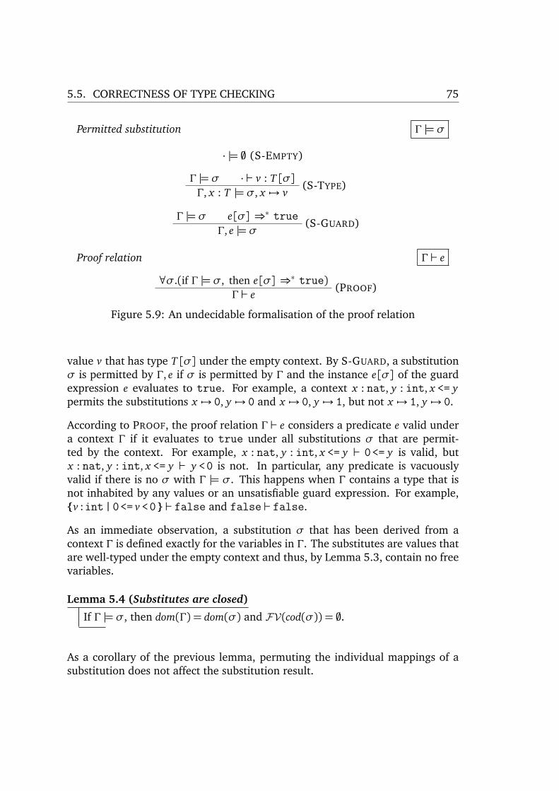
5.5. CORRECTNESS OF TYPE CHECKING 75
Permitted substitution Γ |= σ
· |= ; (S-EMPTY)
Γ |= σ · ` v : T[σ](S-TYPE)
Γ, x : T |= σ, x 7→ v
Γ |= σ e[σ] ⇒∗ true(S-GUARD)
Γ, e |= σ
Proof relation Γ ` e
∀σ.(if Γ |= σ, then e[σ] ⇒∗ true)(PROOF)
Γ ` e
Figure 5.9: An undecidable formalisation of the proof relation
value v that has type T[σ] under the empty context. By S-GUARD, a substitutionσ is permitted by Γ, e if σ is permitted by Γ and the instance e[σ] of the guardexpression e evaluates to true. For example, a context x : nat, y : int, x <= ypermits the substitutions x 7→ 0, y 7→ 0 and x 7→ 0, y 7→ 1, but not x 7→ 1, y 7→ 0.
According to PROOF, the proof relation Γ ` e considers a predicate e valid undera context Γ if it evaluates to true under all substitutions σ that are permit-ted by the context. For example, x : nat, y : int, x <= y ` 0<= y is valid, butx : nat, y : int, x <= y ` y <0 is not. In particular, any predicate is vacuouslyvalid if there is no σ with Γ |= σ. This happens when Γ contains a type that isnot inhabited by any values or an unsatisfiable guard expression. For example,{v:int|0<= v <0} ` false and false ` false.
As an immediate observation, a substitution σ that has been derived from acontext Γ is defined exactly for the variables in Γ. The substitutes are values thatare well-typed under the empty context and thus, by Lemma 5.3, contain no freevariables.
Lemma 5.4 (Substitutes are closed)
If Γ |= σ, then dom(Γ) = dom(σ) and FV(cod(σ)) = ;.
As a corollary of the previous lemma, permuting the individual mappings of asubstitution does not affect the substitution result.

76 CHAPTER 5. TYPE CHECKING QUBECORE
Well-formed contexts ` Γ
` · (C-EMPTY) ` Γ Γ ` T (C-TYPE)` Γ, x : T` Γ Γ ` e : bool (C-GUARD)` Γ, e
Figure 5.10: Well-formed contexts
Corollary 5.5 (Permutation of substitution)
If Γ |= σ1,σ2, then1. for all expressions e, e[σ1,σ2] = e[σ2,σ1]
2. for all types T , T[σ1,σ2] = T[σ2,σ1]
The following lemma establishes a link between the structures of substitutionsand permitting contexts.
Lemma 5.6 (Structure of substitutions)
1. If Γ |= σ1,σ2, then there are contexts Γ1,Γ2 such that Γ = Γ1,Γ2 withdom(Γ1) = dom(σ1) and dom(Γ2) = dom(σ2).
2. If Γ1,Γ2 |= σ, then there are substitutions σ1,σ2 such that σ = σ1,σ2
with dom(Γ1) = dom(σ1) and dom(Γ2) = dom(σ2).
3. Γ1,Γ2 |= σ1,σ2 with dom(Γ1) = dom(σ1) and dom(Γ2) = dom(σ2) iffΓ1 |= σ1, Γ2[σ1] |= σ2.
Figure 5.10 shows the relation ` Γ that defines whether a context Γ is consideredwell-formed. A well-formed context is either empty (·), a well-formed contextΓ extended with declaration of a type T that is well-formed under Γ, or a well-formed context Γ extended with a guard expression e that has type bool under Γ.
The weakening lemma states that the context under which any given fact hasbeen derived may be freely extended with additional variable bindings.

5.5. CORRECTNESS OF TYPE CHECKING 77
Lemma 5.7 (Weakening)
If ` Γ1,Γ2 and Γ1 ` Tx , then1. if Γ1,Γ2 ` e : T , then Γ1, x : Tx ,Γ2 ` e : T .
2. if Γ1,Γ2 ` T , then Γ1, x : Tx ,Γ2 ` T .
3. if Γ1,Γ2 ` T1 <: T2, then Γ1, x : Tx ,Γ2 ` T1 <: T2.
4. if Γ1,Γ2 ` e, then Γ1, x : Tx ,Γ2 ` e.
5. if ∃!n1.Γ1,Γ2 ` n1 = e, then either ∃!n2.Γ1, x : Tx ,Γ2 ` n2 = e with n1 = n2
or Γ1, x : Tx ,Γ2 ` false.
6. if Γ1,Γ2 ` e1 ./ e2 = (v, w)<l> and (Γ1,Γ2 ` vfa l j v j, w j f ) j, thenΓ1, x : Tx ,Γ2 ` e1 ./ e2 = (v′, w′)<l ′> and (Γ1, x : Tx ,Γ2 ` vfa l ′j v′j, w′j f ) j.
Proof : By simultaneous induction over the respective derivations. The proofs of 1.–3.are straightforward inductions.
4. We show that ∀σ.(if Γ1, x : Tx ,Γ2 |= σ, then e[σ] ⇒∗ true), so that the resultfollows from PROOF.
Assume Γ1, x : Tx ,Γ2 |= σ. By Lemma 5.6, Γ1 |= σ1, x : Tx[σ1] |= x 7→ vx , andΓ2[σ1, x 7→ vx] |= σ2. Since x 6∈ FV(Γ2), Γ2[σ1] |= σ2. By Lemma 5.6, Γ1,Γ2 |=σ1,σ2. Since x 6∈ e, e[σ1, x 7→ v,σ2] ⇒∗ true iff e[σ1,σ2] ⇒∗ true. By inversionof PROOF for the assumption Γ1,Γ2 ` e, we already know that ∀σ.(if Γ1,Γ2 |=σ1,σ2, then e[σ1,σ2] ⇒∗ true).
5. There is a unique n with ∀σ.(if Γ1,Γ2 |= σ, then (n = e[σ]) ⇒∗ true). Necessarily,there must be at least one σ with Γ1,Γ2 |= σ and (n = e[σ]) ⇒∗ true.
By Lemma 5.6, Γ1,Γ2 |= σ iff Γ1 |= σ1 and Γ1[σ1] |= σ2. If there is a value vxwith · ` vx : Tx[σ1], then by S-TYPE, Γ1, x : Tx |= σ1, x 7→ vx . As x 6∈ FV(Γ2),Γ2[σ1, x 7→ vx] |= σ2. By Lemma 5.6, Γ1, x : Tx ,Γ2 |= σ1, x 7→ vx ,σ2. Since x 6∈FV(e), (n = e[σ1, x 7→ vx ,σ2]) ⇒∗ true. If there is no vx with · ` vx : Tx[σ1],there is no σ satisfying Γ1, x : Tx ,Γ2 |= σ so that by PROOF, Γ1, x : Tx ,Γ2 ` falseis vacuously true.
6. By induction on the derivation of Γ1,Γ2 ` e1 ./ e2 = (v, w)<l>.
(a) Case J-VECTORS:Γ1,Γ2 ` ev1, .., evn ./ ew1, .., ewn = (ev1, ew1)<l1>, ..,(evn, ewn)<ln>,(Γ1,Γ2 ` ev j : intvec l j , Γ1,Γ2 ` ew j : intvec l j) jBy the hypothesis, the ev j , ew j keep their type under the extended context, sothat J-VECTORS applies, again yielding (ev1, ew1)<l1>,..,(evn, ewn)<ln>. By 4.,(Γ1, x : Tx ,Γ2 ` vfa l j ev j , ew j f ) j.
(b) Case J-ELEMS: Γ1,Γ2 ` ev1, .., evm ./ ew1, .., ewm = ([e],[e′])<n>,Γ1,Γ2 ` ⊕ev1, .., evm = [e], Γ1,Γ2 ` ⊕ew1, .., ewm = [e′]

78 CHAPTER 5. TYPE CHECKING QUBECORE
J-ELEMS relies on the auxiliary rule CONDENSE to statically form the joinedvectors. We inspect the premises of CONDENSE. By the hypothesis, if Γ1,Γ2 `e j : intvec e′j, then Γ1, x : Tx ,Γ2 ` e j : intvec e′j. CONDENSE then tries toguess a constant length n j for each vector e j under the extended context. By5., either the same length as before is guessed or the context is contradictory.If ∃!n j .Γ1, x : Tx ,Γ2 ` n j = e′j, then CONDENSE and subsequently J-ELEMS ap-
ply as before, so that by 4., Γ1, x : Tx ,Γ2 ` vfa n [e],[e′] f . If the contextis contradictory, then by J-EXFALSO, Γ1, x : Tx ,Γ2 ` ev1, .., evn ./ ew1, .., ewn =([],[])<0> and Γ1, x : Tx ,Γ2 ` vfa 0 [],[] f is trivially true.
(c) Case J-EXFALSO: Γ1,Γ2 ` e1 ./ e2 = ([],[])<0>, Γ1,Γ2 ` falseBy 4., Γ1, x : Tx ,Γ2 ` false, so that J-EXFALSO applies again and Γ1, x : Tx ,Γ2 `vfa 0 [],[] f is trivially true.
Similar to weakening, the guard weakening lemma states that the context underwhich a given fact has been derived may be extended with additional guardexpressions. The proof is similar to the proof of the weakening lemma.
Lemma 5.8 (Guard weakening)
If ` Γ1,Γ2 and Γ1 ` eG : bool, then1. if Γ1,Γ2 ` e : T , then Γ1, eG,Γ2 ` e : T .
2. if Γ1,Γ2 ` T , then Γ1, eG,Γ2 ` T .
3. if Γ1,Γ2 ` T1 <: T2, then Γ1, eG,Γ2 ` T1 <: T2.
4. if Γ1,Γ2 ` e, then Γ1, eG,Γ2 ` e.
5. if ∃!n1.Γ1,Γ2 ` n1 = e, then either ∃!n2.Γ1, eG,Γ2 ` n2 = e with n1 = n2 orΓ1, eG,Γ2 ` false.
6. if Γ1,Γ2 ` e1 ./ e2 = (v, w)<l>, and (Γ1,Γ2 ` vfa l j v j, w j f ) j,then Γ1, eG,Γ2 ` e1 ./ e2 = (v′, w′)<l ′> and (Γ1, eG,Γ2 ` vfa l ′j v′j, w′j f ) j
In a similar spirit, the narrowing lemma states that a context under which a facthas been derived may be restricted by confining the types of variables in thecontext. The proof is similar to the proof of the preceding lemmas.

5.5. CORRECTNESS OF TYPE CHECKING 79
Lemma 5.9 (Narrowing)
If ` Γ1, x : Tx ,Γ2 and Γ1 ` T ′x <: Tx , then1. if Γ1, x : Tx ,Γ2 ` e : T , then Γ1, x : T ′x ,Γ2 ` e : T .
2. if Γ1, x : Tx ,Γ2 ` T , then Γ1, x : T ′x ,Γ2 ` T .
3. if Γ1, x : Tx ,Γ2 ` T1 <: T2, then Γ1, x : T ′x ,Γ2 ` T1 <: T2.
4. if Γ1, x : Tx ,Γ2 ` e, then Γ1, x : T ′x ,Γ2 ` e.
5. if ∃!n1.Γ1, x : Tx ,Γ2 ` n1 = e, then either ∃!n2.Γ1, x : T ′x ,Γ2 ` n2 = e withn1 = n2 or Γ1, x : T ′x ,Γ2 ` false.
6. if Γ1, x : Tx ,Γ2 ` e1 ./ e2 = (v, w)<l> and (Γ1, x : Tx ,Γ2 ` vfa l j v j, w j ) j,then Γ1, x : T ′x ,Γ2 ` e1 ./ e2 = (v′, w′)<l ′>, (Γ1, x : T ′x ,Γ2 ` vfa l ′j v′j, w′j f ) j
In QUBECORE, variables can occur in both expressions and types. Due to the vari-able convention 2.3, all bound identifiers are different from the variable to besubstituted. Therefore, the substitution function for QUBECORE is a straightfor-ward extension of the substitution function for the untyped λ-calculus 2.4.The small-step semantics of QUBECORE only requires that values are substitutedinstead of full-blown expressions. We therefore prove a simplified variant of thesubstitution lemma which states that the type of an expression is preserved whenvariables are substituted with values of appropriate types.
Lemma 5.10 (Substitution lemma)
If ` Γ1, x : Tx ,Γ2 and Γ1 ` vx : Tx , then1. if Γ1, x : Tx ,Γ2 ` e : T , then Γ1,Γ2[x 7→ vx] ` e[x 7→ vx] : T[x 7→ vx].
2. if Γ1, x : Tx ,Γ2 ` T , then Γ1,Γ2[x 7→ vx] ` T[x 7→ vx]
3. if Γ1, x : Tx ,Γ2 ` T1<: T2, then Γ1,Γ2[x 7→ vx] ` T1[x 7→ vx]<: T2[x 7→ vx]
4. if Γ1, x : Tx ,Γ2 ` e, then Γ1,Γ2[x 7→ vx] ` e[x 7→ vx].
5. if ∃!n1.Γ1, x : Tx ,Γ2 ` n1 = e, then ∃!n2.Γ1,Γ2[x 7→ vx] ` n2 = e[x 7→ vx]with n1 = n2.
6. if Γ1, x : Tx ,Γ2 ` e1 ./ e2 = (v, w)<l> and (Γ1, x : Tx ,Γ2 ` vfa l j v j, w j f ) j,then Γ1,Γ2[x 7→ vx] ` e1[x 7→ vx] ./ e2[x 7→ vx] = ((v, w)<l>)[x 7→ vx]and (Γ1,Γ2[x 7→ vx] ` (vfa l j v j, w j f )[x 7→ vx]) j
Proof : By simultaneous induction over the respective derivations. Most cases are provedby straightforward induction, similar to the proofs of the previous lemmas.
1. Straightforward induction over typing derivations Γ1, x : Tx ,Γ2 ` e : T , except for
80 CHAPTER 5. TYPE CHECKING QUBECORE
the case T-VAR, where Γ1, x : Tx ,Γ2 ` x ′ : T , x ′ ∈ dom(Γ1, x : Tx ,Γ2)
(a) Case x ′ = x: x ′[x 7→ vx] = vxSince Tx = T , Γ1 ` vx : T . By lemma 5.3, x 6∈ FV(vx) ∪ FV(T ), so thatT[x 7→ vx] = T . By weakening and guard weakening, Γ1,Γ2[x 7→ vx] ` vx : T .
(b) Case x ′ 6= x: x ′[x 7→ vx] = x ′
As x ′ 6= x , x ′ ∈ dom(Γ1,Γ2) and hence, x ′ : T[x 7→ vx] ∈ (Γ1,Γ2[x 7→ vx]). ByT-VAR, Γ1,Γ2[x 7→ vx] ` x ′ : T[x 7→ vx].
2. Straightforward induction over type derivations Γ1, x : Tx ,Γ2 ` T .
3. Straightforward induction over subtype derivations Γ1, x : Tx ,Γ2 ` T1 <: T2.
4. By Γ1, x : Tx ,Γ2 ` e and inversion of PROOF, we know that ∀σ.(if Γ1, x : Tx ,Γ2 |=σ, then e[σ] ⇒∗ true). We show that for all substitutions σ with Γ1,Γ2[x 7→vx] |= σ, there is a substitution σ′ with Γ1, x : Tx ,Γ2 |= σ′, so that the result followsfrom PROOF.Assume Γ1,Γ2[x 7→ vx] |= σ1,σ2. By Lemma 5.6, Γ1 |= σ1, Γ2[x 7→ vx][σ1] |= σ2.By permutation of the substitution, Γ2[σ1, x 7→ vx] |= σ2. From Γ1 |= σ1 andΓ1 ` vx : Tx and by S-TYPE, Γ1, x : Tx |= σ1, x 7→ vx . By Lemma 5.6, Γ1, x : Tx ,Γ2 |=σ1, x 7→ vx ,σ2.
5. By 4., if Γ1, x : Tx ,Γ2 ` n= e, then Γ1,Γ2[x 7→ vx] ` n= e[x 7→ vx].
6. By induction on the derivation of Γ1, x : Tx ,Γ2 ` e1 ./ e2 = (v, w)<l>. Under substi-tution, all rules apply as before.
A subtype relation must be reflexive and transitive, so that subtyping is a pre-order on types.Theorem 5.11 (Subtyping is a preorder)
1. If Γ ` T , then Γ ` T <: T (reflexivity)
2. If Γ ` T1 <: T2 and Γ ` T2 <: T3, then Γ ` T1 <: T3 (transitivity)
Proof : We show reflexivity and transitivity independently.
1. By induction on the derivation of Γ ` T .
(a) Case WF-BTYPE: T = B:Immediate by SUB-BTYPE.
(b) Case WF-FUN: T = x:T1→ T2 with Γ ` T1 and Γ, x : T1 ` T2:By the induction hypothesis, Γ ` T1 <: T1 and Γ, x : T1 ` T2 <: T2. The resultfollows from SUB-FUN.
(c) Case WF-TUP: T = (x:T1,T2) with Γ ` T1 and Γ, x : T1 ` T2:Similar.
(d) Case WF-INTVEC: T = intvec e with Γ ` e : nat:By reflexivity of equality, Γ ` e = e. The result follows from SUB-VEC.

5.5. CORRECTNESS OF TYPE CHECKING 81
(e) Case WF-ARR: T = [T|e1, .., en] with Γ ` T and (Γ ` e j : natvec l j) j:By the hypothesis, Γ ` T <: T . By J-VECTORS, Γ ` e1, .., en ./ e1, .., en =(e1, e1)<l1>, ..,(en, en)<ln>. By reflexivity of equality, (Γ ` vfa l j e j , e j (x , y →x = y)) j. The result follows from SUB-ARR.
(f) Case WF-REFTYPE: T = {x:T ′ | e } with Γ ` T ′ and Γ, x : T ′ ` e : bool:By the hypothesis, Γ ` T ′ <: T ′. By reflexivity of implication, Γ, x : T ′ ` eÖ e.The results follows from SUB-REFTYPE.
2. By induction on the derivations of Γ ` T1 <: T2 and Γ ` T2 <: T3. As each subtypingrule compares two types of the same syntactic form, all three types must have thesame syntactic form. We can thus check the rules individually.
(a) Case SUB-BTYPE: T1 = B, T2 = B, T3 = B. Immediate.(b) Case SUB-FUN: T1 = x:T11→ T12, T2 = x:T21→ T22, T3 = x:T31→ T32 withΓ ` T21 <: T11, Γ, x : T21 ` T12 <: T22 and Γ ` T31 <: T21, Γ, x : T31 ` T22 <: T32By the hypothesis: Γ ` T31 <: T11. By narrowing Γ, x : T21 ` T12 <: T22 we ob-tain Γ, x : T31 ` T12 <: T22. With Γ, x : T31 ` T22 <: T32 and by the hypothesis,Γ, x : T31 ` T12 <: T32. By SUB-FUN, Γ ` x:T11→ T12 <: x:T31→ T32.
(c) Case SUB-TUP: T1 = (x:T11,T12), T2 = (x:T21,T22), T3 = (x:T31,T32) withΓ ` T11 <: T21, Γ, x : T11 ` T12 <: T22 and Γ ` T21 <: T31, Γ, x : T21 ` T22 <: T32By the hypothesis, Γ ` T11 <: T31. By narrowing Γ, x : T21 ` T22 <: T32, we ob-tain Γ, x : T11 ` T22 <: T32. With Γ, x : T11 ` T12 <: T22 and by the hypothesis,Γ, x : T11 ` T12 <: T32. By SUB-TUP, Γ ` (x:T11,T12)<: (x:T31,T32).
(d) Case SUB-VEC: T1 = intvec e1, T2 = intvec e2, T3 = intvec e3 withΓ ` e1 = e2 and Γ ` e2 = e3By transitivity of equality, Γ ` e1 = e3. By SUB-VEC, Γ ` intvec e1 <: intvec e3.
(e) Case SUB-ARR: T1 = [T ′1|e1], T2 = [T ′2|e2], T3 = [T ′3|e3] withΓ ` T ′1 <: T ′2, Γ ` e1 ./ e2 = (u, v)<m>, (Γ ` vfa mi ui , vi (x , y → x=y))i, andΓ ` T ′2 <: T ′3, Γ ` e2 ./ e3 = (v, w)<n>, (Γ ` vfa ni vi , wi (x , y → x=y))iBy the hypothesis, Γ ` T ′1 <: T ′3. We split cases on how the structured vectorsmay have been joined and show that all cases satisfy the premises of SUB-ARR,so that Γ ` [T ′1|e1]<: [T ′3|e3].
i. Case J-EXFALSO, J-EXFALSO: Γ ` falseBy J-EXFALSO, Γ ` e1 ./ e3 = ([],[])<0>. The element-wise equality ofthe empty vectors Γ ` vfa 0 [],[] (x , y → x=y) is trivially valid.
ii. Case J-VECTORS, J-VECTORS: |e1|= |e2|= |e3|= n,(Γ ` e1i : intvec li ,Γ ` e2i : intvec li , Γ ` e3i : intvec li)iBy J-VECTORS, Γ ` e1 ./ e3 = (e11, e31)<l1>, ..,(e1n, e3n)<ln> and by transi-tivity of equality, (Γ ` vfa li e1i , e3i (x , y → x=y))i.
iii. Case J-ELEMS, J-ELEMS: Γ ` ⊕e1 = [e′1], Γ ` ⊕e2 = [e′2], Γ ` ⊕e3 = [e′3]and |e′1|= |e
′2|= |e
′3|= n
By J-ELEMS, Γ ` e1 ./ e3 = ([e′1],[e′3])<n>. By transitivity of equality,Γ ` vfa n [e′1],[e′3] (x , y → x=y).

82 CHAPTER 5. TYPE CHECKING QUBECORE
iv. Case J-VECTORS, J-ELEMS: |e1|= |e2|= m, (Γ ` e1i : intvec li ,Γ ` e2i : intvec li)i, and Γ ` ⊕e2 = [e′2], Γ ` ⊕e3 = [e′3], |e′2|= |e
′3|= n:
The shapes e1, e2 have the same structure. By CONDENSE, Γ ` ⊕e1 = [e′1].By J-ELEMS, Γ ` e1 ./ e3 = ([e′1],[e′3])<n>. By transitivity of equality,Γ ` vfa n [e′1],[e′3] (x , y → x=y).
v. Case J-ELEMS, J-VECTORS: Similar(f) Case SUB-REF: T1 = {x:T ′1 | e1 }, T2 = {x:T ′2 | e2 }, T3 = {x:T ′3 | e3 } withΓ ` T ′1 <: T ′2, Γ, x : T ′1 ` e1Ö e2 and Γ ` T ′2 <: T ′3, Γ, x : T ′2 ` e2Ö e3:By the hypothesis Γ ` T ′1 <: T ′3. By narrowing Γ, x : T ′2 ` e2 Ö e3 we obtainΓ, x : T ′1 ` e2 Ö e3. By transitivity of implication, Γ, x : T ′1 ` e1 Ö e3 and thusby SUB-REF, Γ ` {x:T ′1 | e1 }<: {x:T ′3 | e3 }.
The following lemma captures the intuition that evaluation does not affect thevalidity of a predicate.Lemma 5.12 (Preservation of validity under evaluation)
If Γ ` eE[e] and e ⇒ e′, then Γ ` eE[e′].
Proof : From the assumption and by inversion of PROOF, we obtain ∀σ. (if Γ |= σ,then eE[e][σ] ⇒∗ true). By Theorem 4.20, evaluation is deterministic and therefore,eE[e][σ] ⇒∗ true iff eE[e′][σ] ⇒∗ true. The result follows from PROOF.
Similarly, evaluation has no effect on types.Lemma 5.13 (Equivalence of types under evaluation)
If Γ ` T[e] and e ⇒ e′, then Γ ` T[e] ≡ T[e′], i. e., Γ ` T[e′] <: T[e] andΓ ` T[e]<: T[e′].
Proof : By induction on type derivations Γ ` T .
1. Case WF-BTYPE: T = BB contains no expressions.
2. Case WF-FUN: T = x:T1[e]→ T2[e], Γ ` T1[e], Γ, x : T1[e] ` T2[e]By the hypothesis, Γ ` T1[e′]≡ T1[e] and Γ, x : T1[e] ` T2[e′]≡ T2[e]. By SUB-FUN,Γ ` x:T1[e′]→ T2[e′]≡ x:T1[e]→ T2[e].
3. Case WF-TUP: T = (x:T1[e],T2[e]), Γ ` T1[e], Γ, x : T1[e] ` T2[e]By the hypothesis, Γ ` T1[e′]≡ T1[e] and Γ, x : T1[e] ` T2[e′]≡ T2[e]. By SUB-TUP,Γ ` (x:T1[e′],T2[e′])≡ (x:T1[e],T2[e]).
4. Case WF-INTVEC: T = intvec eE[e], Γ ` eE[e] : nat.By Theorem 4.20, evaluation is deterministic. Therefore, eE[e] and eE[e′] will eval-uate to the same value under all permitted substitutions, so that Γ ` eE[e] = eE[e′].By SUB-VEC, Γ ` intvec eE[e]≡ intvec eE[e′].

5.5. CORRECTNESS OF TYPE CHECKING 83
5. Case WF-ARRAY: T = [T ′[e]|es[e]], Γ ` T ′[e], (Γ ` es j[e] : natvec el j) jBy the hypothesis, Γ ` T ′[e′] ≡ T ′[e]. Evaluation does not affect the structure ofa structured vector, so that by J-VECTORS, Γ ` es1[e′], .., esm[e′] ./ es1[e], .., esm[e] =(es1[e′], es1[e])<el1>, ..,(esm[e′], esm[e])<elm>. By Theorem 4.20, evaluation is de-terministic. Therefore, for each j, es j[e] and es j[e′] will evaluate to the samevalue under all permitted substitutions, so that Γ ` es j[e′] ~=el j
es j[e]. By SUB-ARR,
Γ ` [T ′[e′]|es[e′]]≡ [T ′[e]|es[e]].
6. Case WF-REFTYPE: T = {x:T ′[e]| eE[e]}, Γ ` T ′[e], Γ ` eE[e] : bool.By the hypothesis, Γ ` T ′[e′] ≡ T ′[e]. By Theorem 4.20, evaluation is determinis-tic. Therefore, eE[e] and eE[e′] will evaluate to the same value under all permit-ted substitutions, so that by reflexivity of implication Γ, x : T ′[e] ` eE[e] Ö eE[e′]and Γ, x : T ′[e] ` eE[e′] Ö eE[e]. By SUB-REFTYPE, Γ ` {x:T ′[e′]| eE[e′]} ≡{x:T ′[e]| eE[e]}
With all these facts in hand, we can now prove the preservation theorem.Theorem 5.14 (Preservation of types under evaluation)
If Γ ` e : T and e ⇒ e′, then Γ ` e′ : T .
Proof : By induction on type derivations Γ ` e : T . We split cases on the potentialevaluation steps.
1. Case T-SUB: Γ ` e : T ′, Γ ` T ′ <: T , Γ ` TBy the hypothesis, Γ ` e′ : T ′ and thus the result follows from T-SUB.
2. Case T-VAR: e = x . There is no e′ with e ⇒ e′.
3. Case T-CONST: e = c. e is a value.
4. Case T-ABS: e = fun x:T1→ e′. e is a value.
5. Case T-APP: e = e1 e2, Γ ` e1 : (x:T1→ T2), Γ ` e2 : T1, T = T2[x 7→ e2]
(a) Case E-APP1: e1 ⇒ e′1, e′ = e′1 e2By the hypothesis, Γ ` e′1 : (x:T1→ T2). The result follows from T-APP.
(b) Case E-APP2: e1 = v1, e2 ⇒ e′2, e′ = v1 e′2By T-APP, Γ ` e′ : T2[x 7→ e′2]. By Lemma 5.13, Γ ` T2[x 7→ e′2] <: T2[x 7→ e2],so that the result follows from T-SUB.
(c) Case E-APPABS: e1=fun x:T1→ eb, e2= v2, Γ, x : T1 ` eb : T2, e′ = eb[x 7→ v2]By Lemma 5.10, Γ ` e′ : T2[x 7→ v2].
(d) Case E-PRFAPP1: e1 = f 1, e2 = v2, f 1(v2) ⇒δ v, e′ = vBy Axiom 5.2, Γ ` v : T2[x 7→ v2].
(e) Case E-PRFAPP2: e1 = f 2 v1, e2 = v2, f 2(v1, v2) ⇒δ v, e′ = v. Similar.
6. Case T-LET: e = let x = e1 in e2, Γ ` e1 : T1, Γ, x : T1 ` e2 : T , Γ ` T
(a) Case E-LETR: e1 ⇒ e′1, e′ = let x = e′1 in e2The result follows from the induction hypothesis and T-LET.

84 CHAPTER 5. TYPE CHECKING QUBECORE
(b) Case E-LET: e1 = v1, e′ = e2[x 7→ v1]By the substitution lemma, Γ ` e′ : T[x 7→ v1]. Since Γ ` T , x is not free in Tand thus Γ ` e′ : T .
7. Case T-COND: e = if :T ep then et else ee, Γ ` T , Γ ` ep : bool,Γ ` et : T , Γ ` ee : T
(a) Case E-COND: ep ⇒ e′p, e′ = if :T e′p then et else eeThe result follows from the induction hypothesis and T-COND.
(b) Case E-CONDT: ep = true, e′ = et . Immediate.(c) Case E-CONDE: ep = false, e′ = ee. Immediate.
8. Case T-COERCE: e = (e1:T), Γ ` T , Γ ` e1 : T
(a) Case E-COERCES: e1 ⇒ e′1, e′ = (e′1:T)The result follows from the induction hypothesis and T-COERCE.
(b) Case E-COERCE: e1 = v1, e′ = v1. Immediate.
9. Case T-TUP: e = (e1, e2:(x:T1,T2)), Γ ` (x:T1,T2), Γ ` e1 : T1,Γ ` e2 : T2[x 7→ e1], T = (x:T1,T2)
(a) Case E-TUP1: e1 ⇒ e′1, e′ = (e′1, e2:(x:T1,T2))By the hypothesis, Γ ` e′1 : T1. By Lemma 5.13, Γ ` T2[x 7→ e1] <: T2[x 7→ e′1],so that by T-SUB, Γ ` e2 : T2[x 7→ e′1]. The result follows from T-TUP.
(b) Case E-TUP2: e1 = v1, e2 ⇒ e′2, e′ = (v1, e′2:(x:T1,T2))By the hypothesis, Γ ` e′2 : T2[x 7→ v1]. The result follows from T-TUP.
10. Case T-UNPACK: e = let (x1, x2) = e1 in e2, Γ ` e1 : (x:T1,T2),Γ, x1 : T1, x2 : T2[x 7→ x1] ` e2 : T , Γ ` T
(a) Case E-UNPACKE: e1 ⇒ e′1, e′ = let (x1, x2) = e′1 in e2The result follows from the induction hypothesis and T-UNPACK.
(b) Case E-UNPACK: e1 = (v1, v2:(x:T1,T2)), e′ = e2[x1 7→ v1][x2 7→ v2]By inversion of T-TUP, Γ ` v1 : T1, Γ ` v2 : T2[x 7→ v1]. By the substitutionlemma 5.10 and because x1 is not free in T , Γ, x2 : T2[x 7→ x1][x1 7→ v1] `e2[x1 7→ v1] : T . Since T2[x 7→ x1][x1 7→ v1] ≡ T2[x 7→ v1], and by thesubstitution lemma, Γ ` e2[x1 7→ v1][x2 7→ v2] : T .
11. Case T-VECTOR: e = [e], (Γ ` e j : int) j, T = {x:intvec |e|| x ~=|e| [e]}By E-SEQ and E-VECTOR, e ⇒seq e′ with |e| = |e′| so that e′ = [e′]. By T-VECTOR,Γ ` e′ : {x:intvec |e|| x ~=|e| [e′]}. The result follows from Lemma 5.13 andT-SUB.
12. Case T-VSEL: e = ev.(ei), Γ ` ev : intvec en, Γ ` ei : {x:int|0 <= x < en },T = {x:int| x = ev.(ei)}
(a) Case E-VSELV: ev ⇒ e′v, e′ = e′v.(ei)By the hypothesis, Γ ` e′v : intvec en. By T-VSEL, Γ ` e′ : {x:int| x = e′v.(ei)}.The result follows from Lemma 5.13 and T-SUB.
(b) Case E-VSELI: ev = vv, ei ⇒ e′i , e′ = vv.(e′i)
5.5. CORRECTNESS OF TYPE CHECKING 85
By the hypothesis, Γ ` e′i : {x:int|0 <= x < en }. According to T-VSEL, Γ ` e′ :{x:int| x = vv.(e′i)}. The result follows from Lemma 5.13 and T-SUB.
(c) Case E-VSEL: ev = [c], 0≤ ei = i < |c|, e′ = ciBy T-CONST, Γ ` e′ : {x:int| x = ci }. The result follows from Lemma 5.13and T-SUB.
13. Case T-VMOD: e = ev.(ei)← ee, Γ ` ev : intvec en, Γ ` ei : {x:int|0 <= x < en },Γ ` ee : int, T = {x:intvec en | x ~=en
ev.(ei)← ee }
(a) Case E-VMV: ev ⇒ e′v, e′ = e′v.(ei)← ee
(b) Case E-VMI: ev = vv, ei ⇒ e′i , e′ = vv.(e′i)← ee
(c) Case E-VME: ev = vv, ei = vi, ee ⇒ e′e, e′ = vv.(vi)← e′eThe results follow from the hypothesis, T-VMOD, Lemma 5.13, and T-SUB.
(d) Case E-VMOD: ev = [c], 0≤ ei = i < |c|, ee = ce, e′ = [c[i 7→ ce]]By T-VECTOR, Γ ` e′ : {x:intvec |c|| x ~=|c| [c[i 7→ ce]]}. The result followsfrom Lemma 5.13 and T-SUB.
14. Case T-VEC: e = vec en ee, Γ ` en : nat, Γ ` ee : int, T = {x:intvec en | x = vec en ee }
(a) Case E-VECL: en ⇒ e′n, e′ = vec e′n eeBy the hypothesis, Γ ` e′n : nat. By T-VEC, Γ ` e′ : {x:intvec e′n | x = vec e′n ee }.The result follows from Lemma 5.13 and T-SUB.
(b) Case E-VECE: en = vn, ee ⇒ e′e, e′ = vec vn veBy the hypothesis, Γ ` e′e : int. By T-VEC, Γ ` e′ : {x:intvec vn | x = vec vn e′e }.The result follows from Lemma 5.13 and T-SUB.
(c) Case E-VEC: 0≤ en = n, ee = ce, e′ = [ce, .., ce]By T-VECTOR, Γ ` e′ : {x:intvec n| x ~=n [ce, .., ce]}. The result follows fromLemma 5.13 and T-SUB.
15. Case T-VMAP: e = vmap en ev (x → eb), Γ ` en : nat, (Γ ` ev j : intvec en) j,x : int ` eb : int, T = {x ′:intvec en | x ′ ~=en
vmap en ev (x → eb)}
(a) Case E-VMAPL: en ⇒ e′n, e′ = vmap e′n ev (x → eb)By the hypothesis, Γ ` e′n : nat. According to the typing rule T-VMAP, Γ `e′ : {x ′:intvec e′n | x ′ ~=e′n
vmap e′n ev (x → eb)}. The result follows fromLemma 5.13 and T-SUB.
(b) Case E-VMAPV: en = vn, ev ⇒seq e′v, e′ = vmap vn e′v (x → eb)By the hypothesis, (Γ ` e′v j : intvec vn) j. According to T-VMAP, Γ ` e′ :
{x ′:intvec vn | x ′ ~=vnvmap vn e′v (x → eb)}. The result follows from Lemma
5.13 and T-SUB.(c) Case E-VMAP: 0≤ n= en, ev = [c0], ..,[cm], |ci|= n, e′ = [eb0, .., ebn−1] where
eb j = eb[x0 7→ c0 j]..[xm 7→ cmj]By Lemma 5.10, (· ` eb j : int) j. According to the typing rule T-VECTOR, Γ `e′ : {x ′:intvec n| x ′ ~=n [eb0, .., ebn−1]}. The result follows from Lemma 5.13and T-SUB.
16. Case T-VFA: e = vfa en ev (x → eb), Γ ` en : nat, (Γ ` ev j : intvec en) j, x : int `

86 CHAPTER 5. TYPE CHECKING QUBECORE
eb : bool, T = {x ′:bool| x ′ ↔ vfa en ev (x → eb)}
(a) Case E-VFAL: en ⇒ e′n, e′ = vfa e′n ev (x → eb)By the hypothesis, Γ ` e′n : nat. According to the typing rule T-VFA, Γ ` e′ :{x ′:bool| x ′ ↔ vfa e′n ev (x → eb)}. The result follows from Lemma 5.13and T-SUB.
(b) Case E-VFAV: en = vn, ev ⇒seq e′v, e′ = vfa vn e′v (x → eb)By the hypothesis, (Γ ` e′v j : intvec vn) j. According to the typing rule T-VFA,
Γ ` e′ : {x ′:bool| x ′ ↔ vfa vn e′v (x → eb)}. The result follows fromLemma 5.13 and T-SUB.
(c) Case E-VFA: 0 ≤ n = en, ev = [c0], ..,[cm], e′ = eb0 & .. & ebn−1 where eb j =eb[x0 7→ c0 j]..[xm 7→ cmj]By Lemma 5.10, (· ` eb j : bool) j. By T-APP, T-CONST, Γ ` e′ : {x ′:bool| x ′↔eb0 & .. & ebn−1 }. The result follows from Lemma 5.13 and T-SUB.
17. Case T-ARR: e = [e : T ′|[n]], Γ ` T ′, (Γ ` e j : T ′) j, T = [T ′|[n]]By E-SEQ and E-ARR, e ⇒seq e′ with |e|= |e′|. By the induction hypothesis,(Γ ` e′j : T ′) j. Thus, the result follows by T-ARR.
18. Case T-SEL: e = ea.[ei], Γ ` ea : [T|es], Γ ` es ./ ei = (s, v)<r>,(Γ ` vfa r j s j , v j (s, i→ 0<=i & i<s)) j(a) Case E-SELA: ea ⇒ e′a, e′ = e′a.[ei]
By the hypothesis, Γ ` e′a : [T|es], so that the result follows from T-SEL.
(b) Case E-SELI: ei ⇒seq e′i , e′ = ea.[e′i]By the hypothesis, the type of each ei j is preserved, so that e′i has the same
structure as ei. Hence, Γ ` es ./ e′i = (s, v′)<r>. According to Lemma 5.12,(Γ ` vfa r j s j , v′j (s, i→ 0<=i&i<s)) j. By T-SEL, Γ ` e′ : T .
(c) Case E-SEL: ea = [v : T|[n]], ei = [i1], ..,[im], e′ = v(ι n (i1,..,im)).
By inversion of T-ARR, (Γ ` v j : T ) j and therefore Γ ` e′ : T .
19. Case T-MOD: e = ea.[ei]← ee, Γ ` ea : [T ′|es], Γ ` ee : T ′, Γ ` es ./ ei = (s, v)<r>,(Γ ` vfa r j s j , v j (s, i→ 0<=i & i<s)) j, T = [T ′|es]
(a) Case E-MA: ea ⇒ e′a, e′ = e′a.[ei]← eeBy the hypothesis, Γ ` e′a : [T ′|es], so that the result follows from T-MOD.
(b) Case E-MI: ei ⇒seq e′i , e′ = ea.[e′i]← ee
By the hypothesis, the type of each ei j is preserved, so that e′i has the same
structure as ei. Hence, Γ ` es ./ e′i = (s, v′)<r>. By Lemma 5.12, (Γ `vfa r j s j , v′j (s, i→ 0<=i&i<s)) j. The result follows from T-MOD.
(c) Case E-ME: ee ⇒ e′e, e′ = ea.[ei]← e′eBy the hypothesis, Γ ` e′e : T ′, so that the result follows from T-MOD.
(d) Case E-MOD: ea = [v : T ′|[n]], ei = [i1], ..,[im], ee = ve,e′ = [v[ι n (i1, .., im) 7→ ve] : T ′|[n]].

5.5. CORRECTNESS OF TYPE CHECKING 87
By inversion of T-ARR, (Γ ` v j : T ′) j. Thus, by T-ARR, Γ ` e′ : [T ′|[n]]. SinceΓ ` ea : [T ′|es], we know that Γ ` [T ′|[n]] <: [T ′|es], and therefore byT-SUB, Γ ` e′ : [T ′|es].
20. Case T-RSHP: e = reshape et ea, (Γ ` et j : natvec el j) j, Γ ` ea : [T ′|es],(Γ ` vfa er j es j (x → 0< x)) j, T = [T ′|et]
(a) Case E-RS: et ⇒seq e′t , e′ = reshape e′t ea
By the hypothesis, (Γ ` e′t j : natvec el j) j. By T-RESHAPE, Γ ` e′ : [T ′|e′t]. By
Lemma 5.13, Γ ` [T ′|e′t]<: [T ′|et]. The result thus follows from T-SUB.(b) Case E-RA: ea ⇒ e′a, e′ = reshape et e′a
By the hypothesis, Γ ` e′a : [T ′|es]. The result follows from T-RESHAPE.(c) Case E-RSHP: et = [i1], ..,[im], ea = [v : T ′|[n]], (0< n j) j,
e′ = [v′ : T ′|[i1, .., im]], v′k = vk mod∏
n
By T-ARR, Γ ` e′ : [T ′|[i1, .., im]]. By J-ELEMS, Γ ` [i1, .., im] ./ [i1], ..,[im]=([i1, .., im],[i1, .., im])<r> and Γ ` vfa r [i1, .., im],[i1, .., im] (x , y → x = y)holds because of the reflexivity of equality. By SUB-ARR, Γ ` [T ′|[i1, .., im]]<:[T ′|[i1], ..,[im]], so that by T-SUB, Γ ` e′ : T .
21. Case T-GEN: e = gen :Tb es with x → eb, Γ ` Tb, (Γ ` es j : natvec er j) j,Γ, x1 : indexvec er1 es1, .., xm : indexvec erm esm ` eb : Tb, T = [Tb|es]
(a) E-GENS: es ⇒seq e′s, e′ = gen :Tb e′s with x → eb
By the hypothesis, (Γ ` e′s j : natvec er j) j. By T-GEN, Γ ` e′ : [Tb|e′s]. By
Lemma 5.13, Γ ` [Tb|e′s]<: [Tb|es]. The result follows from T-SUB.
(b) E-GEN: es = [n1], ..,[nm], e′ = [e′b : Tb|[n1, .., nm]], e′bk = eb[x j 7→ [i j]] j
By construction, (Γ ` [i j] : indexvec er j es j) j. By the substitution lemma 5.10,(Γ ` ebk : Tb)k. By T-ARR, Γ ` e′ : [Tb|[n1, .., nm]]. By rule J-ELEMS,Γ ` [n1, .., nm] ./ [n1], ..,[nm]= ([n1, .., nm],[n1, .., nm])<r> andΓ ` vfa r [n1, .., nm],[n1, .., nm] (x , y → x = y) holds because of the reflexiv-ity of equality. By SUB-ARR, Γ ` [Tb|[n1, .., nm]] <: [Tb|[n1], ..,[nm]], sothat by T-SUB, Γ ` e′ : T .
22. Case T-LOOP: e = loop xa:T = ea; es with x → eb, Γ ` T , (Γ ` es j : natvec er j) j,Γ ` ea : T , Γ, x1 : indexvec er1 es1, .., xm : indexvec erm esm, xa : T ` eb : T
(a) Case E-LOOPS: es ⇒seq e′s, e′ = loop xa:T = ea; e′s with x → ebBy the hypothesis, (Γ ` e′s j : natvec er j) j. By T-LOOP, Γ ` e′ : T .
(b) Case E-LOOP: (es j = [n j]) j, e′ = fp−1 (...( f0 ea)) with p =∏
(n1, .., nm) andfk = fun x:T → eb[x j 7→ [i j]] j such that ι (n1, .., nm) (i1, .., im) = kBy construction, (Γ ` [i j] : indexvec er j es j) j. By the substitution lemma 5.10,Γ, xa : T ` eb[x j 7→ [i j]] j : T . By T-FUN, Γ ` fk : T → T . By several applica-tions of T-APP, Γ ` e′ : T .

88 CHAPTER 5. TYPE CHECKING QUBECORE
The canonical forms lemma recapitulates the possible forms the values of a giventype may have. The lemma is a straightforward observation from the syntax ofvalues, the types of constants, and the typing rules.Lemma 5.15 (Canonical forms)
1. If v is a value with · ` v : bool then v is either true or false.
2. If v is a value with · ` v : int then v ∈ Z.
3. If v is a value with · ` v : x:T1 → T2 then v = f 1, v = f 2, v = f 2 v1, orv = fun x:T → e.
4. If v is a value with · ` v : (x:T1,T2) then v = (v1, v2:(x:T1,T2)).
5. If v is a value with · ` v : intvec e then v = [n] with e ⇒∗ |n| and(ni ∈ Z)i.
6. If v is a value with · ` v : [T|e1, .., em] then v = [v : T|[n]] whereeach element vi is a value with · ` vi : T and (ni ≥ 0)i, |v| =
∏
n.Furthermore, (ei ⇒∗ [si])i with s1, .., sm = n.
7. If v is a value with · ` v : {x:T | e } then v is any value v′ with · ` v′ : Tand e[x 7→ v′] ⇒∗ true.
Finally, we are ready to prove the progress theorem for QUBECORE.
Theorem 5.16 (Progress)
If · ` e : T , then e is a value or there is some e′ with e ⇒ e′.
Proof : By induction on typing derivations · ` e : T .
1. Case T-SUB: e = e, · ` e : T ′, · ` T ′ <: T , · ` TThe result follows directly from the induction hypothesis.
2. Case T-VAR: e = xe is not closed.
3. Case T-CONST: e = ce is a value.
4. Case T-ABS: e = fun x:T → e′
e is a value.
5. Case T-APP: e = e1 e2, · ` e1 : x:T1→ T2, · ` e2 : T1By the hypothesis, either e1 is a value or it can make an evaluation step; e2 similar.If e1 is not a value, then E-APP1 applies. If e1 is a value and e2 is not,then E-APP2applies. If both expressions are values, then by the canonical forms lemma either
• e1 = f 2 then e = f 2 v2 is a value, or• e1 = f 1 and E-PRFAPP1 applies because of axiom 5.2, or

5.5. CORRECTNESS OF TYPE CHECKING 89
• e1 = f 2 v1 and E-PRFAPP2 applies because of axiom 5.2, or• e1 = fun x:T ′→ e′ and E-ABSAPP applies.
6. Case T-LET: e = let x = e1 in e2By the hypothesis, e1 is a value or it can make an evaluation step. If e1 is not avalue, then E-LETE applies, else E-LET applies.
7. Case T-COND: e = if e1 then e2 else e3, · ` e1 : boolBy the hypothesis, e1 is a value or it can make an evaluation step. If e1 is not avalue, then E-COND applies. If e1 is a value, then by the canonical forms lemma, itis either true or false. Thus either E-CONDT or E-CONDE applies.
8. Case T-COERCE: e = (e1:T1)By the hypothesis, e1 is a value or it can make an evaluation step. If e1 is not avalue, then E-COERCES applies, else E-COERCE applies.
9. Case T-TUP: e = (e1, e2:(x:T1,T2))By the hypothesis, e1, e2 are values or they can make an evaluation step. If e1 is nota value, then E-TUP1 applies. If e1 is a value and e2 is not, then E-TUP2 applies. Ifboth expressions are values, then e is a value.
10. Case T-UNPACK: e = let (x1, x2) = e1 in e2By the hypothesis, e1 is a value or it can make an evaluation step. If e1 is not avalue, then E-UNPACKE applies. If e1 is a value, then by the canonical forms lemmae1 = (v1, v2:(x:T1,T2)) and hence, E-UNPACK applies.
11. Case T-VECTOR: e = [e], (· ` e j : int) jBy the hypothesis, the expressions e are either values of or they can make an eval-uation step. When an expression is not a value, then E-SEQ and E-VECTOR apply.When all expressions are values, they must all be integers (canonical forms lemma)and therefore, the vector is a value.
12. Case T-VSEL: e = ev.(ei), · ` ev : intvec el , · ` ei : {x:int|0<=x<el }By the hypothesis, e and ei are either values or they can make an evaluation step. Ifev is not a value, then E-VSELV applies. If ev is a value and ei is not, then E-VSELIapplies. If both expressions are values, then, by the canonical forms lemma, evmust be a vector [n] with el ⇒∗ |n| and ei must be an integer i with 0≤ i < |n|, sothat E-VSEL applies.
13. Case T-VMOD: Similar.
14. Case T-VEC: e = vec en ee, · ` en : nat, · ` ee : intBy the hypothesis, en and ee are either values or they can make an evaluation step.If en is not a value, then E-VECL applies. If en is a value and ei is not, then E-VECEapplies. If both expressions are values, then by the canonical forms lemma, en mustbe an integer n with 0≤ n and ei must be an integer, so that E-VEC applies.
15. Case V-MAP: e = vmap en e (x → eb), |e|= |x |, · ` en : nat, (· ` e j : intvec en) jBy the hypothesis, en and the expressions e are either values or they can make anevaluation step. If en is not a value, then E-VMAPL applies. If en is a value, and anei is not, then E-SEQ and E-VMAPV apply. If all expressions are values then, by the

90 CHAPTER 5. TYPE CHECKING QUBECORE
canonical forms lemma, en must be an integer n with 0≤ n and each expression e jmust be an integer vector [m j] with |m j|= n. Since also |e|= |x |, E-VMAP applies.
16. Case T-VFA: e = vfa en e (x → eb). Similar.
17. Case T-ARRAY: e = [e : T|[n]], (· ` e j : T ) jBy the hypothesis, each expressions ei is either a value of can make an evaluationstep. When some expression ei is not a value, then E-SEQ and E-ARR apply. Whenall expressions are values, the array is itself a value.
18. Case T-SEL: e = ea.[e1, .., em], · ` ea : [T|es1, .., esn], · ` es1, .., esn ./ e1, .., em =(s, v)<r>, (· ` vfa ri s j , v j (s, i→ 0<=i & i<s)) jBy the hypothesis, ea and the ei are either values or they can make an evaluationstep. If ea is not a value, E-SELA applies. If ea is a value, but some ei is not, thenE-SEQ and E-SELI apply. If all subexpressions are values, then, by the canonicalforms lemma, ea must be an array value [v : T|[n]] with (esi ⇒∗ [si])i so thats1, .., sm = n. Moreover, each index vector e j must be an integer vector [i j]. Theremaining preconditions ensure that the shapes es and ei can be joined and that theindex vectors describe a valid position in ea, i. e., |i1, .., in|= |n| and (0≤ (i1, .., in) j <n j) j. Thus, E-SEL applies.
19. Case T-MOD: e = ea.[ei]← ee. Similar.
20. Case T-RSHP: e = reshape e1, .., em ea, (· ` ei : natvec _)i, · ` ea : [T ′|es1, .., esn],(· ` vfa er j es j (x → 0< x)) jBy the hypothesis, ea and the ei are either values or they can make an evaluationstep. If some ei is not a value, then E-SEQ and E-RS apply. If all ei are values, butea is not, then E-RA applies. If all subexpressions are values, then, by the canonicalforms lemma, ea must be an array value [v : T|[n]] with (esi ⇒∗ [si])i so thats1, .., sm = n. By the precondition, (0 < n j) j. Moreover, each shape vector e j mustbe a vector of natural numbers [i j]. Therefore, E-RSHP applies.
21. Case T-GEN: e = gen :Tb es with x → eb, · ` Tb, (· ` es j : natvec er j) j,x1 : (indexvec er1 es1), .., xm : (indexvec erm esm) ` eb : TbBy the hypothesis, the esi are either values or they can make an evaluation step.If some ei is not a value, then E-SEQ and E-GENS apply. If all subexpressions arevalues, then by the canonical forms lemma, each esi must be a vector of naturalnumbers and therefore E-GEN applies.
22. Case T-LOOP: e = loop xa:T = ea; es with x → eb, · ` T , (· ` es j : natvec er j) j,· ` ea : T , x1 : (indexvec er1 es1), .., xm : (indexvec erm esm), xa : T ` eb : TBy the hypothesis, the esi are either values or they can make an evaluation step. Ifsome ei is not a value, then E-SEQ and E-LOOPS apply. If all subexpressions arevalues, then by the canonical forms lemma, each esi must be a vector of naturalnumbers and therefore E-LOOP applies.
The progress theorem states that each closed and well-typed term is either avalue or can make an evaluation step. As stated by the preservation theorem,
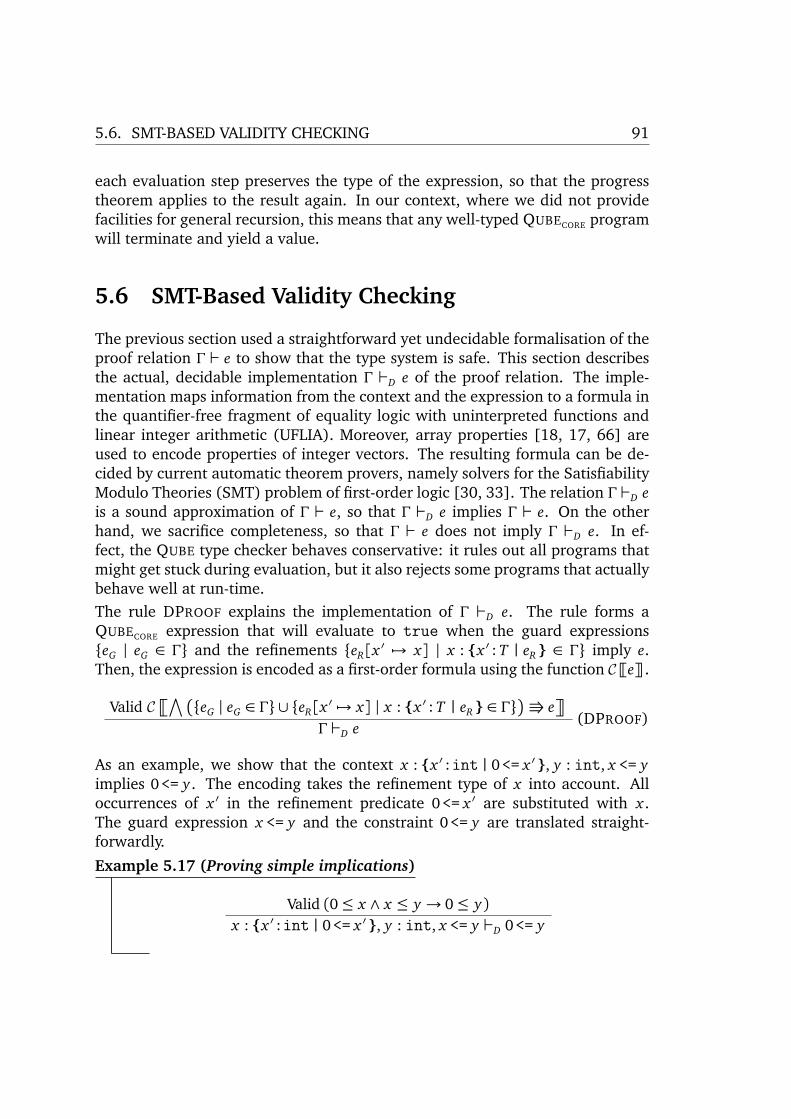
5.6. SMT-BASED VALIDITY CHECKING 91
each evaluation step preserves the type of the expression, so that the progresstheorem applies to the result again. In our context, where we did not providefacilities for general recursion, this means that any well-typed QUBECORE programwill terminate and yield a value.
5.6 SMT-Based Validity Checking
The previous section used a straightforward yet undecidable formalisation of theproof relation Γ ` e to show that the type system is safe. This section describesthe actual, decidable implementation Γ `D e of the proof relation. The imple-mentation maps information from the context and the expression to a formula inthe quantifier-free fragment of equality logic with uninterpreted functions andlinear integer arithmetic (UFLIA). Moreover, array properties [18, 17, 66] areused to encode properties of integer vectors. The resulting formula can be de-cided by current automatic theorem provers, namely solvers for the SatisfiabilityModulo Theories (SMT) problem of first-order logic [30, 33]. The relation Γ `D eis a sound approximation of Γ ` e, so that Γ `D e implies Γ ` e. On the otherhand, we sacrifice completeness, so that Γ ` e does not imply Γ `D e. In ef-fect, the QUBE type checker behaves conservative: it rules out all programs thatmight get stuck during evaluation, but it also rejects some programs that actuallybehave well at run-time.The rule DPROOF explains the implementation of Γ `D e. The rule forms aQUBECORE expression that will evaluate to true when the guard expressions{eG | eG ∈ Γ} and the refinements {eR[x ′ 7→ x] | x : {x ′:T | eR } ∈ Γ} imply e.Then, the expression is encoded as a first-order formula using the function C¹eº.
Valid C�∧�
{eG | eG ∈ Γ} ∪ {eR[x ′ 7→ x] | x : {x ′:T | eR } ∈ Γ}�
Ö e�
(DPROOF)Γ `D e
As an example, we show that the context x : {x ′:int|0<= x ′ }, y : int, x <= yimplies 0<= y. The encoding takes the refinement type of x into account. Alloccurrences of x ′ in the refinement predicate 0<= x ′ are substituted with x .The guard expression x <= y and the constraint 0<= y are translated straight-forwardly.
Example 5.17 (Proving simple implications)
Valid (0≤ x ∧ x ≤ y → 0≤ y)x : {x ′:int|0<= x ′ }, y : int, x <= y `D 0<= y

92 CHAPTER 5. TYPE CHECKING QUBECORE
The example only contains variables and applications of function symbols thatare readily available in the quantifier-free UFLIA fragment of first-order logic.In general however, the encoding must also translate the other QUBECORE ex-pressions, such as let-bindings, function definitions as well as vector and arrayexpressions. We now explain the translation in more detail.The languages of SMT solvers such as YICES [33] or Z3 [30] are variants ofmany-sorted first-order logic which generalises first-order logic as presented inChapter 3. Similar to programming languages that use types to classify expres-sions, many-sorted logic uses sorts to classify terms. For the sake of simplicity, wedo not consider sorts or well-sorted terms. We just assume that there are primi-tive sorts bool and int and that all our terms are well-sorted. Terms of sort boolare called formulas, so that a syntactic distinction between terms and formulasis redundant. Although the syntax of many-sorted logic permits arbitrary nest-ings of terms and formulas, both can be disentangled so that the conventionalstructure of first-order formulas can be restored.In many-sorted logic, a term t is either a variable x , an application f (t1, ..., tn)of a function symbol f to terms, a conditional term ite(t1, t2, t3), or a quantifiedterm ∀x . t or ∃x . t. Constants are nullary function symbols. The boolean functionsymbols >, ⊥, ¬, ∨, ∧, ∨, →, and ↔ have the usual meaning. The sort intintroduces function symbols for the integers Z, the predicate symbols =, 6=, <,≤, ≥, >, and the linear arithmetic functions +, −, and Z·. Moreover, there isa special binary function symbol t1[t2] for reading an element with the integerindex t2 from an array t1.Figure 5.11 shows the encoding function ¹eº(κ). The function takes a QUBECORE
expression e and a function κ, which maps QUBECORE variables to logic terms, forprocessing local variable definitions. The result (t, T ) consists of a term t thatapproximates the expression and a set T of additional constraints, which arealso terms. The encoding function is defined using pattern matching: the firstequation whose left-hand side matches the expression applies.The encoding function C¹·º used in DPROOF is defined in terms of ¹·º(·):
C¹eº=∧
({t} ∪ T ) where (t, T ) = ¹eº(κ0)
The function κ0 : x → t yields a logical variable x for every QUBECORE variable x .The operation ·[· ← ·] alters a function κ such that κ[x ← t](x) = t. A variablex always represents a fresh uninterpreted function symbol.¹xº(κ) encodes the variable x by applying κ. For let-bindings let x = e1 in e2,the encoding follows the operational semantics. First, e1 is translated to (t1, T1).Then, e2 is encoded under κ[x ← t1]which gives (t2, T2) so that the let-expressioncan be encoded as (t2, T1 ∪ T2).

5.6. SMT-BASED VALIDITY CHECKING 93
Logical encoding of QUBECORE expressions ¹eº(κ) = (t, T )
¹xº(κ) = (κ(x),;)�
let x = e1 in e2�
(κ) = (t2, T1 ∪ T2)
where (t1, T1) =�
e1�
(κ),(t2, T2) =
�
e2�
(κ[x ← t1])¹trueº(κ) = (>,;)¹falseº(κ) = (⊥,;)
¹nº(κ) = (n,;)¹not eº(κ) = (¬t, T ) where (t, T ) = ¹eº(κ)
◦ ∈ {↔,&,|}.�
e1 ◦ e2�
(κ) = (t1 ◦ t2, T1 ∪ T2) where (t i , Ti) =�
ei�
(κ)
◦ ∈ {=,<, ...}.�
e1 ◦ e2�
(κ) = (t1 ◦ t2, T1 ∪ T2) where (t i , Ti) =�
ei�
(κ)
◦ ∈ {+,-}.�
e1 ◦ e2�
(κ) = (t1 ◦ t2, T1 ∪ T2) where (t i , Ti) =�
ei�
(κ)
¹n * eº(κ) = (n ∗ t, T ) where (t, T ) = ¹eº(κ)
◦ ∈ {*,/,%}. ¹e ◦ nº(κ) = (t ◦n, T ) where (t, T ) = ¹eº(κ)�
e1 e2�
(κ) = (t1(t2), T1 ∪ T2) where (t i , Ti) =�
ei�
(κ)�
if :T e1 then e2 else e3�
(κ) = (ite(t1, t2, t3), T1 ∪ T2 ∪ T3)
where (t i , Ti) =�
ei�
(κ)�
(e1, e2:T)�
(κ) = ( x ,;)�
let (x1, x2) = e1 in e2�
(κ) =�
e2�
(κ)
¹(e:T)º(κ) = ¹eº(κ)�
e1.(e2)�
(κ) = (t1[t2], T1 ∪ T2) where (t i , Ti) =�
ei�
(κ)�
e1.(e2)← e3�
(κ) = ( x , { x[t2] = t3 ∧∀ j. j 6= t2→ x[ j] = t1[ j]} ∪ T )
where (t i , Ti) =�
ei�
(κ), T = T1 ∪ T2 ∪ T3
¹[e]º(κ) = ( x , { x[i] = t i}i ∪⋃
iTi) where (t i , Ti) =
�
ei�
(κ)�
vec e1 e2�
(κ) = ( x , { y = t2 ∧∀ j. 0≤ j < t1→ x[ j] = y} ∪ T1 ∪ T2)
where (t i , Ti) =�
ei�
(κ)�
vmap en e (y → eb)�
(κ) = ( x , {∀ j. 0≤ j < tn→ x[ j] = tb[yi 7→ t i[ j]]i} ∪ T )
where T = Tn ∪⋃
iTi , (t i , Ti) =
�
ei�
(κ)�
vfa en e (y → eb)�
(κ) = ( x , { x ↔∀ j. 0≤ j < tn→ tb[yi 7→ t i[ j]]i} ∪ T )
where T = Tn ∪⋃
iTi , (t i , Ti) =
�
ei�
(κ)
¹eº(κ) = ( x ,;)
Figure 5.11: A mapping from QUBECORE expressions to logical formulas. The firstequation whose left-hand side matches the expression applies.

94 CHAPTER 5. TYPE CHECKING QUBECORE
Booleans and integer constants map to the corresponding logical constants. Sim-ilarly, we encode applications of boolean operators, (linear) arithmetic opera-tors, and conditional expressions as applications of the equivalent interpretedfunctions. All other functions map to uninterpreted function symbols by thebottom-most rule.Tuples (e1, e2:T) are abstractly represented as uninterpreted functions x . Simi-larly, the encoding of unpack-expressions let (x1, x2) = e1 in e2 merely takes e2
into account, abstracting away from the relationship between the variables x1, x2
and the expression e1. The encoding function ignores type annotations (e:T).In contrast, the encoding function emphasises the accurate representation of vec-tors and vector operations. Selections e1.(e2) are encoded as logical array readst1[t2]. The vector modification e1.(e2) ← e3 represents a vector that is equalto e1 at all position except e2, where it is e3. We thus encode the vector modi-fication as a new logical array x with the additional constraints x[t2] = t3 and∀ j. j 6= t2 → x[ j] = t1[ j]. In a similar spirit, we encode vector constructors [e]as fresh arrays x with x[ j] = t j for all j and constant-value vector expressionsvec e1 e2 as arrays x with y = t2 and ∀ j. 0≤ j < t1→ x[ j] = y.Vectors defined by map expressions vmap en e (y → eb) are also converted tonew logical arrays x . Modelling the operational semantics of vmap, the array isconstrained such that each element x[ j]must equal tb[yi 7→ t i[ j]]i, i. e., every yi
in tb gets replaced with t i[ j]. The encoding of vector predicates vfa en e (x →eb) is similar, but introduces x as a truth variable that is constrained by theuniversally quantified formula ∀ j. 0≤ j < tn→ tb[x i 7→ t i[ j]]i.All other expressions, namely abstractions, and the expressions from QUBE[], areencoded as uninterpreted functions x .We now prove some essential properties of the transformation. Given an expres-sion, the encoding function yields a term and a set of constraints that are liftedout of their original context. In the presence of universal quantifiers, it is crucialthat no term that depends on a quantified variable is moved out of the scope ofthe quantifier.Proposition 5.18 (Expressions under vmap and vfa yield no constraints)
For map operations vmap en e (x → eb) and predicates vfa en e (x → eb),encoding of the eb yields an empty constraint set, i. e.,
�
eb�
(κ) = (tb,;)
Proof : Constraints are only generated by the encoding rules for [ · ], ·.( · ) ← ·, vec,vmap, and vfa. The typing rules treat eb as a restricted expression and thereby ensurethat none of the above expressions may appear in eb.
5.6. SMT-BASED VALIDITY CHECKING 95
An encoded formula may contain some universal quantifiers and thus may notbe immediately processed by an SMT solver. We show that the universally quan-tified terms all belong to the decidable array property fragment [18], so that theentire formula can be transformed into an equisatisfiable quantifier-free formulaby means of the decision procedure outlined in Section 3.4.
Proposition 5.19 (Quantified terms are array properties)
The universally quantified terms that result from encoding vector expressionsare array properties.
Proof : Only the encoding rules for ·.( · ) ← ·, vec, vmap, and vfa emit universallyquantified terms. We inspect the rules individually.
1. Case e1.(e2)← e3:The quantified term is ∀ j. j 6= t2 → x[ j] = t1[ j]. The index guard j 6= t2 is ashorthand for j ≤ t2−1∨ t2+1≤ j. By construction, e2 and thus t2 cannot dependon j, which allows us to abstract out t2 out of the index guard as a new variable.In the value constraint x[ j] = t1[ j], the index variable j is only used to select intoarrays.
2. Case vec e1 e2:The quantified term is ∀ j. 0 ≤ j < t1 → x[ j] = y. Similar to the above case, theindex guard may be rewritten as 0 ≤ j ≤ t1 − 1 and t1 may be abstracted out as itcannot depend on j. The value constraint obeys the required grammar.
3. Case vmap en e (x → e):The quantified term is ∀ j. 0 ≤ j < tn → x[ j] = tb[yi → t i[ j]]i. The index guardmay be transformed to meet requirements as in case 2. Since eb is a restrictedexpression, the term tb can only contain constants, the variables x as integers,logical and arithmetic functions and if-then-else terms. In particular, tb cannotby itself reference j. Therefore, substituting the variables x i with t i[ j] yields awell-formed value constraint.
4. Case vfa en e (x → e): Similar.
The encoding function is accurate for boolean expressions, integers and linearinteger operations, vector expressions and let-bindings. All other expressionsare soundly abstracted away with uninterpreted function symbols. When onlyexpressions of the former group are used in program positions where the proofrelation is used to reason about values, the type checker will not report any falsetype errors. Specifically, these positions are type refinements, length expres-sions in vector types, shape expressions in array types, conditional predicates,function arguments or tuple components when a value of some refinement typeis expected, length expressions in vec, vmap, and vfa, vector indices, shape

96 CHAPTER 5. TYPE CHECKING QUBECORE
expressions in reshape, gen, loop, and array index vectors. Despite the ex-tensive list, many interesting array programs can be typed. Some examples willbe shown in Section 8. Moreover, in cases where the proof machinery fails toaccurately reason about the value of a complex expression, appropriate run-timechecks can be inserted manually.
Summary
This chapter presented the type system of QUBECORE and gave proof of its safety.However, even with SMT-based constraint proving, the presented rules are notimmediately suitable for implementation. Responsible for this is the subsump-tion rule T-SUB which applies to every expression arbitrarily often. In contrast,all other rules are syntax directed: for every expression, there is one and onlyone type checking rule that matches that expression. Thus, to implement a ter-minating type checking algorithm, it is only necessary to tame the subsumptionrule.QUBECORE is constructed such that type checking never requires to guess an ap-propriate supertype for an expression. Instead, the language elements are an-notated with these types. For example the conditional if :T e then et else ee
provides a common supertype T for both branches. Thus, in all situations wherethe declarative rules use the subsumption rule to appropriately elevate the typeof an expression, it is sufficient to check whether the type is a subtype of therequired type and we can therefore eliminate T-SUB.

Part III
The QUBE Programming Language
97


6The QUBE Programming Language
This chapter describes the actual syntax of the QUBE programming language.The syntax of QUBE is heavily inspired by OCAML [69], a popular dialect of theML family of functional languages. Programmers familiar with OCAML shouldbe able to quickly learn QUBE, too. Aimed to be a practical language for ar-ray programming with dependent types, QUBE extends QUBECORE with a richerexpression syntax, more base types, some syntactic sugar, an ML-style modulesystem [83], and support for stateful computations and I/O. The latter two ex-tensions were added to the QUBE compiler by Florian Büther in the course ofhis Diploma thesis [20]. Hence, this chapter only gives a brief overview of thesefeatures and refers the reader to the aforementioned thesis for details.The remainder of the chapter is organised as follows: Section 6.1 explains theexpression syntax of QUBE and how it extends QUBECORE. Section 6.2 outlinesthe module system of QUBE. Finally, Section 6.3 explains how QUBE integratesstateful computations and I/O operations by means of uniqueness types.
6.1 Expression Syntax
This section explains the expression syntax of QUBE and how it is different fromQUBECORE. Fig. 6.1 specifies an (abstract) grammar of QUBE expressions in ex-tended Backus-Naur form.To facilitate general-purpose computations, QUBE provides the additional base
99

100 CHAPTER 6. THE QUBE PROGRAMMING LANGUAGE
types char, float, and double along with the required constants, arithmeticoperations, and conversion operations.
QUBE generalizes the unary functions of QUBECORE to functions of arbitrary arity.The n-ary function type has the form x1:T1. ... xn:Tn → Tn+1. The syntax offunction types allows the compiler to statically determine how many argumentsare required for an exact application of a given operator. The correspondingabstraction has the form fun x1:T1 ... xn:Tn :Tn+1 → e, where the declaration ofthe return type :Tn+1 is optional. The syntax of the extended application thatallows an operator to be applied to multiple operands is e e1 ... em, where m maydiffer from the arity of e. The following example illustrates the definition of aternary function and its function type.
Example 6.1 (Function with multiple arguments)
(fun x:int y:int z:int :int → x+y+z) : x:int. y:int. z:int → int
Variables that denote binary functions can be enclosed in backticks and be usedas infix operators. For example, x ‘add‘ y is equivalent to add x y .
Similar to the generalisation of functions, QUBE generalises pairs to (dependent)tuples with n components for n≥ 2. The dependent tuple type of length n has theform (x1:T1,...,xn−1:Tn−1,Tn). The syntax of the dependent tuple constructoris (e1,...,en:(x1:T1,...,xn−1:Tn−1,Tn)), whereas a non-dependent tuple maysimply be specified as (e1,...,en). The example shows how dependent triplescan be used to represent arrays of different rank and shape in a uniform way.
Example 6.2 (Dependent triples)
(1,[5] ,[1,2,3,4,5|[5]] : (r:nat, s:natvec r, [int|s]))(2,[2,2],[1,2,3,4|[2,2]] : (r:nat, s:natvec r, [int|s]))
The type annotation at the conditional expression is optional in QUBE. In mostexpressions if ep then et else ee, either the type of et is a supertype of the typeof ee, or vice versa. In these cases, the compiler will automatically assume thegreater type as the type of the conditional.
The let construct of QUBE combines the let and unpack expressions fromQUBECORE and adds support for mutually recursive function definitions. The non-recursive binding let p1 = e1 and ... and pn = en in en+1 evaluates the expressionse1, .., en in arbitrary order and matches the results with the patterns p1, .., pn suchthat all variables from the patterns are bound to values in en+1. Patterns may bevariables x and tuple patterns (p1,...,pm) for m≥ 2.
The recursive binding let rec p1 = e1 and ... and pn = en in en+1 defines aset of mutually recursive functions under the restriction that all patterns pi are

6.1. EXPRESSION SYNTAX 101
T ::= B�
� {x:T | e }�
�
��
x:�
T.�
x:�
T → T Types�
� (��
x:�
T,+T)
�
� intvec e�
� [T|e�
,e
]| X�
e
B ::= bool�
� int�
� char�
� float�
� double Base types
e ::= c�
� x�
� fun�
x:T+ �:T
�
→ e�
� e�
e+ Expressions
�
� (e:T)�
� (e�
,e+�:T
�
)�
� if�
:T�
e then e else e�
� let�
rec�
l b�
and l b
in e�
� e.(e)�
� e.(e)← e�
� vec e e�
� vmap e�
,e
(x�
,x
→ e)�
� vfa e�
,e
(x�
,x
→ e)�
� [�
e�
,e��
:T��
|[�
Z�
,Z�
]�
]�
� e.[e�
,e
]�
� e.[e�
,e
]← e�
� reshape e�
,e
e�
� gen�
:T�
e�
,e
with g�
� loop x�
:T�
= e; e�
,e
with g
l b ::= p = e�
� x�
x:T+ �:T
�
= e Let bindingsp ::= x
�
� (p�
,p+) Patterns
g ::= vp�
,vp
→ e�
� rp�
,rp
→ e | vp�
,vp
→ e Generatorsvp ::= x
�
� [�
x�
,x�
] Vector patternsrp ::=
�
@r as�
vp Range patternsr ::= e
�
� e..�
� ..e�
� e..e Ranges
Figure 6.1: The expression syntax of QUBE
mere variables x i and that all right-hand side expressions ei are abstractionsfun x1 : T1 ... xn : Tn : Tn+1→ e that provide a result type.
As a convenience notation, QUBE provides a special let binding for functiondefinitions. The binding x f x1 : T1 ... xn : Tn : Tn+1 = e is equivalent to writingx f = fun x1 : T1 .. xn : Tn : Tn+1 → e. In both notations, the result type is onlyrequired for declaring recursive functions. To illustrate the let expression, wedefine the well-known mutually recursive functions even and odd.
Example 6.3 (Mutually recursive functions)
let rec even n:nat :bool = if n = 0 then true else odd (n-1)and odd n:nat :bool = if n = 0 then false else even (n-1)in even 4
The vector and array expressions of QUBE differ very little from their counter-parts in QUBECORE. Most notably, the vector constructor and the array constructorhave been fused into a common expression. The element type and shape anno-

102 CHAPTER 6. THE QUBE PROGRAMMING LANGUAGE
tations are optional. If the type annotation is missing, the compiler determinesa common supertype of all elements. For empty array constructors, the elementtype defaults to int. If the shape annotation is missing, the array constructorwill be assumed to define a rank 1 array. Vectors with integer elements will begiven an intvec type, as described by rule T-VECTOR in Figure 5.7. Via an ad-ditional subtyping rule, the compiler allows integer vectors to be used as rank 1integer arrays. In QUBE, vmap and vfa do not require the vector length as anargument.The gen and loop expressions of QUBE employ a restricted form of patternmatching on index vectors to allow the elements in a convex sub-region of theindex space to be computed from a different expression than all other elements.An array comprehension of the formgen s with @lb..ub as x → e | x’ → e’
specifies an array of shape vector s, whose elements are either computed fromthe expression e or from the default expression e’. Which of these two expres-sions is chosen depends on the element’s index vector. If the index vector iswithin the range specified by the range pattern @lb..ub, where the lower boundvector lb is inclusive and the upper bound vector ub is exclusive, e is chosen, oth-erwise e’ is taken. In situations where the length of the index vector is constant,QUBE allows the index vector to be alternatively specified as a vector pattern [x].The element type of gen and the accumulator type of loop are optional as thecompiler can in many cases determine an appropriate type itself. To illustraterange and vector patterns, we define an operation that concatenates two vectorsof doubles.Example 6.4 (Range and vector patterns)
let concat m:nat n:nat a:[double|[m]] b:[double|[n]] =gen [m+n] with| @[0]..[m] as x → a.[x]| [i] → b.[[i-m]]
6.2 Module System
To support large-scale programming beyond individual expressions, QUBE fea-tures an elaborate module system [20, 83]. The system supports separate names-paces, separate compilation, information hiding, and interfacing with foreignfunctions.A module consists of a signature that describes all the types and values providedby the module and a structure that contains the actual definitions. Each source

6.2. MODULE SYSTEM 103
M ::= struct�
b
end�
�
�
m.
m�
� M:I Module expressionsb ::= type X
�
x:T
= T�
� let�
rec�
l b�
and l b
Bindings�
� structure m = M�
� signature i = I�
� open�
m.
m�
� external x : T = symbol
I ::= sig�
d
end�
�
�
m.
i Interface expressionsd ::= type X
�
x:T�
= T�
�
� val x : T Declarations�
� structure m: I�
� signature i = I�
� open�
m.
m�
� external x : T = symbol
T ::= ...�
�
�
m.
X Typese ::= ...
�
�
�
m.
x Expressions
Figure 6.2: The module syntax of QUBE
code file A.q implicitly defines a structure A. Similarly, a source code file A.qiimplicitly defines a signature A. Alternatively, structures and signatures can bedefined explicitly, even inside of other structures.Figure 6.2 shows the module syntax of QUBE. In the figure, four different kindsof identifiers are used. As before, the metavariables x and X represent value andtype identifiers, respectively. The metavariable m stands for a module identifierand i stands for an interface identifier. Module identifiers must begin with anuppercase letter, all other identifiers must begin with a lowercase letter.To navigate through the module hierarchy, both value identifiers and type iden-tifiers are extended with a module path. For example, Cpx.make selects the valuemake from a module Cpx.A module expression M is either a structure definition struct bs end that pack-ages together related bindings bs, a path m1.... mn.m that selects a structure mfrom a module tree, or a module expression of the form M : I that restricts theinterface of the module M to the interface I .The binding type X x1 : T1 ... xn : Tn = Tn+1 defines a new type X that takesarguments x i of type Ti as an abbreviation of the right-hand side type Tn+1. Sim-ilar to the let expression, the let binding simultaneously defines a number of(potentially recursive) values.A binding of the form structure m = M binds a structure m that is defined bythe module expression M . Similarly, a binding of the form signature i = I bindsa signature i that is defined by the interface expression I .A binding open m1.... mn.m makes all names from the module m1.... mn.m avail-able in the current structure without the module path.Finally, a binding of the form external x : T = symbol declares an externally

104 CHAPTER 6. THE QUBE PROGRAMMING LANGUAGE
structure Cpx = structtype t = (double,double)let make re:double im:double = (re,im)let re c:t = let (re,_) = c in relet im c:t = let (_,im) = c in im(* ... *)
end : sigtype tval make : double. double → tval re : t → doubleval im : t → double(* ... *)
end
Figure 6.3: An example module for complex numbers
defined function x of type T that is implemented by the linker symbol symbol.Analogue to module expressions, an interface expression is either a signaturedefinition sig ds end that packages a list ds of declarations, or a path m1.... mn.ithat selects an interface i from a module tree.
The declarations of a signature abstractly describe the bindings of a structure. Atype declaration may omit the implementation of the type to create an abstractdata type. A declaration of the form val x : T merely indicates the existence ofa value x of type t. Similarly, a structure can only be declared to have a certaininterface. In contrast, the signature, open, and external declarations areequivalent to the corresponding bindings.
To illustrate some of the module syntax, Figure 6.3 shows an example moduleCpx that provides basic support for complex numbers. The structure implementscomplex numbers as pairs of double and defines the necessary constructor anddestructor functions. The module is sealed by a signature that hides the imple-mentation type of complex numbers such that values of type Cpx.t can only bemanipulated by functions from Cpx.
6.3 Stateful Computations
QUBE expressions are referentially transparent, i. e., an expression will alwaysevaluate to the same result when applied to the same arguments. While theabsence of state and side-effects makes it easy to reason about QUBE expressions,additional measures are required to mimic the behaviour of imperative programs

6.3. STATEFUL COMPUTATIONS 105
T ::= TC
�
� *TC
�
� ?TC
�
� u^TC TypesTC ::= B
�
� {x:T | e }�
�
��
x:�
T.�
x:�
T → T Core Types�
� (��
x:�
T,+T)
�
� intvec e�
� [T|e�
,e
]| X�
e
e ::= ...�
� e!(e)�
� e!(e)← e�
� e![�
e,
e]�
� e![�
e,
e]← e Expressions
Figure 6.4: Syntax for uniqueness types and destructive array operations
that manipulate the machine state or interact with the execution environment.Similar to the programming languages CLEAN and SAC, QUBE uses uniquenesstypes [9] to incorporate side-effects into the referentially transparent setting.The implementation most closely resembles the approach described in [32].A variable with a unique type must be referenced at most once. Unique objectsare thus explicit representations of state. To manipulate such a state, a functionmust consume the corresponding unique object and produce a new unique ob-ject that represents the new state. The data dependencies between producersand consumers of unique objects then implicitly enforce the desired sequentialevaluation of unique expressions.Figure 6.4 shows the syntax extensions for uniqueness types. The types havebeen refined such that every type consists of a core type TC and a uniquenessattribute. Core types are essentially the types as defined in Section 6.1. A type*TC is unique. The absence of a uniqueness attribute implicitly makes a typeshared. A uniqueness variable u makes the type u^TC polymorphic with respectto the uniqueness attribute. The type checker determines an appropriate instanceof u depending on how the corresponding value is used. The notation ?TC is aconvenience notation for u^TC where u is a fresh variable.Each element of a data structure has its own uniqueness. In order to avoidillegal sharing of unique elements, the uniqueness propagation rule must beobeyed [84]: if a unique object is stored in a data structure, the data structurebecomes unique as well.To enable interactive programs, QUBE defines an abstract type *world whosevalues represent states of the execution environment. The function main, whichserves as the entry point of a QUBE program, must have type *world → *world.The type captures the intuition that an interactive program transforms the exe-cution environment from an initial to a final state. Using the library functionIo.print_endline of type string. *world → *world, we can write a HelloWorld program.Example 6.5 (Hello World)
let main w:*world = Io.print_endline "Hello␣World" w

106 CHAPTER 6. THE QUBE PROGRAMMING LANGUAGE
let swap n:nat arr:*[int|[n]] i:(index n) j:(index n) =let (arr,ai) = arr![[i]] inlet (arr,aj) = arr![[j]] inlet arr = arr![[i]] ← aj inlet arr = arr![[j]] ← ai inarr
Figure 6.5: Destructive swapping of array elements
In the context of array programs, uniqueness types have a desirable second ap-plication. Since a unique array type describes an array that has at most onereference to it, modifications of this array may be performed destructively. Thus,the asymptotic complexity of array modification drops from O(n) to O(1).QUBE provides a custom set of expressions to access and modify unique arrays.The unique vector selection e!(e) and the unique array selection e![e, ..., e]take unique arrays and shared indices. In order to preserve the array reference,the expressions return a fresh reference to the array in addition to the selectedelement. The unique vector modification e!(e)← e and the unique array modi-fication e![e, ..., e]← e take unique arrays, shared indices, and shared substituteelements.To illustrate destructive array modification, Figure 6.5 defines a function swapthat takes a unique array and two valid array indices i and j. The operationuses unique array selections to select the elements at the positions i and j, re-spectively. Afterwards, the array is updated destructively and the final referenceto the array is returned.
Summary
This chapter presented the syntax of the QUBE programming language. Basedon QUBECORE, the language provides a number of features for practical array pro-gramming with dependent types. The module system of QUBE allows complexprograms to be decomposed into smaller and more manageable modules that as-semble related definitions. QUBE uses the module system to provide an extensivestandard library of predefined functions. Via uniqueness types, QUBE supportsstateful computations such as I/O and destructive array updates without losingreferential transparency.

7Language Implementation
QUBE is implemented by a compiler that translates QUBE programs into codefor the Low-Level Virtual Machine (LLVM) which in turn emits machine-specificassembly language. The compiler was implemented by Florian Büther, MarkusWeigel, Sebastian Hungerecker, and myself.
The remainder of this chapter is organized as follows: Section 7.1 characterisesthe design goals of the QUBE compiler. Section 7.2 gives an overview of the com-piler architecture and describes the individual phases of the compilation process.The implementation dynamically represents multidimensional arrays as meresequences of elements. Section 7.3 explains how the QUBE compiler uses thedependent array types to statically augment intermediate programs with infor-mation about array ranks and shapes wherever these are required for evaluation.
7.1 Design of the QUBE Compiler
The design of the QUBE compiler aims at translating QUBE programs into well-performing executables. A secondary goal was to explore how to use the richtype information to produce even better code.
Most visible to the user, the compiler uses the types to statically detect programerrors such as array-boundary violations and give appropriate type error mes-sages. Type checking is performed in collaboration with a Satisfiability Modulo
107

108 CHAPTER 7. LANGUAGE IMPLEMENTATION
Theories (SMT) solver. Programs that pass the type checker are known not to ex-hibit program errors. In consequence, the compiler can avoid inserting dynamicchecks such as array bounds checks into the program.QUBE’s type system is monomorphic. Therefore, all basic values have unboxedrepresentations. Only closures, tuples, and arrays are allocated on the heap.Multidimensional arrays are represented solely by their linear data vectors. In-stead of also providing the corresponding shape vectors at run-time, the compileruses the shape expressions from the array types to statically annotate the pro-gram with shape information wherever necessary. The process will be describedin more detail in Section 7.3.Integer vectors have a pre-eminent role in array programming. They representshapes and allow us to index elements from multidimensional arrays. Unfor-tunately, the overhead of allocating a vector on the heap just to select a singlearray element is prohibitive. To avoid integer vectors from manifesting at run-time, the QUBE compiler employs two strategies. First, whenever the length ofan integer vector is statically known, the compiler represents the vector by itsindividual elements. Operations on these vectors can in most cases be unrolled,resulting in a number of scalar computations. Second, the compiler implementsindex vector elimination (IVE) [12], a technique develop in the context of the SACcompiler [42] that replaces linear operations on index vectors with equivalentoperations on scalar offsets.QUBE is a higher-order language that supports first-class functions and nestedfunction declarations. Inner functions may refer to variables that are bound inthe surrounding function. The QUBE compiler uses lambda lifting [60] to elim-inate free variables from inner functions. For each free variable, the procedureintroduces an additional function argument that must be passed at every appli-cation. The closed functions are moved to the top-level.The implementation of curried function applications takes advantage of QUBE’sn-ary function types. As the arity of any given function f is statically known, thecompiler can determine whether an application f e1 .. en provides too few, toomany, or the right number of arguments. If the number of arguments matchesthe function’s arity, an exact call is made. If there are too many arguments, thecompiler splits the application so that first an exact call is made whose result isthen applied to the remaining arguments. If the application has too few argu-ments, the compiler generates a closure that combines a tuple (e1, .., en) with apointer to a new function that takes the tuple and the remaining arguments sothat it can make an exact call to f .Another important feature of functional programming languages is automaticmemory management. The language implementation is responsible for allocat-ing space for new data structures and releasing the memory once the data struc-

7.2. COMPILATION AT A GLANCE 109
tures are no longer used. Currently, the QUBE compiler relies on the Boehm-Dehmers-Weiser conservative garbage collector [16] for storage reclamation. Inthe future however, we would like to replace it with a memory managementscheme based on reference counting, since this would allow us to safely performdestructive array updates even in the context of immutable arrays [45, 94].
The QUBE compiler targets the Low-Level Virtual Machine (LLVM) [68], a com-piler infrastructure that supports a variety of processor architectures. LLVMtakes programs in a machine-independent typed assembly language and per-forms extensive compile-time optimisations. The result is either statically com-piled to machine code or stored as bytecode for interpretation (aided by just-in-time compilation). A feature that makes compiling to LLVM particularly in-teresting is its support for tail-call optimisation (TCO) [62], a technique thatsubstitutes function calls in tail position with more efficient jump instructionsinto the called functions.
As LLVM can use the C calling conventions, the generated object files can belinked with native libraries. Interfacing between QUBE and C programs is straight-forward due to the similarities between the representations of QUBE data struc-tures and the corresponding data structures in C. The interoperation works inboth directions: QUBE programs can access library functions written in C and,vice versa, QUBE functions can serve as the trusted computational kernels ofprograms written in any other language that can interface with C.
The QUBE compiler itself is written in OCAML [69, 22], a popular language inthe ML family of programming languages [70, 75]. OCAML offers inductivedata types and facilities to define recursive functions over these types by patternmatching. In conjunction with type inference and automatic memory manage-ment, these features make OCAML well-suited for compiler construction.
7.2 Compilation at a Glance
This section describes the compilation process of the QUBE compiler. Fig. 7.1gives an overview of the compilation. The blocks represent the individual compi-lation phases that lower the source program to a native object file a.out througha series of intermediate representations.
The compiler accepts a QUBE program as a source file suffixed with .q. Scanningand parsing of the program yields a Parsetree, an abstract syntax tree that closelyresembles the source program.
Type checking is performed in collaboration with the YICES theorem prover [33].The implementation of the proof relation Γ `D e encodes the context and the

110 CHAPTER 7. LANGUAGE IMPLEMENTATION
Compilation process
Parsing
Type checking SMT solver
Normalization
Optimization
Index transformation
Lambda lifting
Memory management
Code generation
LLVM
.q
a.out
Function inliningConstant foldingCommon subexpression eliminationDead code removal
Parsetree
Typedtree
Coretree
Coretree
Indextree
Indextree
Memtree
LLVM code
UFLIA formula
UNSAT/Model
Figure 7.1: The compilation process of QUBE

7.2. COMPILATION AT A GLANCE 111
negated property not e as a logical formula in the decidable UFLIA1 fragmentof first-order logic as described in Section 5.6. When the SMT solver yieldsunsatisfiable then e is valid under Γ and thus the program is type correct. In casethat the SMT solver finds the encoded formula satisfiable, it reports a model,i. e., an assignment of the program variables in Γ that satisfies the encoding ofnot e. Since e may thus be invalid under Γ, the program is rejected with anappropriate type error message.Well-typed programs are emitted by the type checker in an intermediate repre-sentation called Typedtree. This abstract syntax tree still largely resembles thesource program with a few notable differences. First, all user-defined typesare replaced by their definitions. Second, all bound identifiers are uniquely re-named. Third, to admit descriptor-free representation, all language elementsthat deal with vectors or arrays are annotated with expressions that representthe vector lengths, array rank and shapes, respectively. The descriptor-free arrayrepresentation and the required compile-time annotations will be described inmore detail in section 7.3.The Normalisation phase systematically eliminates complex subexpressions fromthe syntax tree, yielding the intermediate representation Coretree. Similar toadministrative normal form [37], Coretree only allows functions to be applied totrivial arguments, called atoms, which are either constants or identifiers. Morecomplex expressions must only appear on the right-hand side of a let-binding.Thus, complex subexpressions are abstracted out of their original context andbound to fresh variables.Due to its regular structure, the Coretree representation is well-suited for programoptimisation. The side-effect free nature of (well-typed) QUBE programs allowsto straightforwardly apply a host of compiler optimisations without changingthe program semantics. Currently, the QUBE compiler performs the followinghigh-level program optimisations most of which are well-known from compilerconstruction text books [1, 3, 47]:
• Function inlining: non-recursive functions whose size do not exceed acertain threshold are inlined.
• Partial evaluation: the compiler reduces applications of the built-in logicand arithmetic operations to constant arguments. Conditionals with con-stant predicates are reduced to the adequate branch. Unpack expressionsare reduced when the definition of the tuple is known. For vectors andarrays that are defined by a constructor, selections and modifications withconstant index vectors and reshape operations with constant shape vec-tors are reduced. For vectors of known length, instances of vmap and vfa
1uninterpreted functions and linear integer arithmetic

112 CHAPTER 7. LANGUAGE IMPLEMENTATION
are expanded. Similarly, instances of gen and loop are expanded for smallshapes.
• Common subexpression elimination: identical right-hand sides of let-bindings are eliminated to avoid redundant computations.
• Dead code removal: the compiler eliminates all bindings of unreferencedvariables as these cannot contribute to the program result.
After program optimisation, the compiler phase index transformation lowers themultidimensional QUBE arrays to linear arrays that can be mapped to actualcomputing hardware. In particular, index vectors into multidimensional arraysare transformed into scalar offsets into the linear array representation. By meansof index vector elimination [12], the compiler converts many linear operationson heap-allocated integer vectors into equivalent scalar operations that can beperformed in processor registers. The compiler phase maps the syntax tree to arepresentation called Indextree that dispenses with dependent types in favour ofsimple types.The next phase Lambda lifting [60] eliminates nested function definitions. Theprocedure augments inner functions with additional arguments for each freevariable and modifies all applications of these functions to pass the necessaryvalue. The closed functions are then moved out of their original context to thetop-level.The Memory management phase augments the intermediate code with instruc-tions that explicitly allocate and modify memory. In effect, the purely functionalQUBE programs are transformed into stateful programs that perform computa-tions as a sequence of modifications of the machine state.As the final stage of the QUBE compiler, code generation transforms the syntaxtree into code for the Low-Level Virtual Machine (LLVM) [68] which in turnemits machine-specific object code.
7.3 Descriptor-Free Array Representation
Array ranks and shape vectors are essential for the evaluation of array programs:for a matrix a:[int|[m,n]] stored in row-major order, the element a.[[i,j]]is located in the linear memory representation of a at the offset i · n + j. Toprovide rank and shape vector wherever necessary, language implementationstypically associate each array with an array descriptor that is maintained at run-time in addition to the array itself. A descriptor-based array representation of atakes the form of a tuple <2,[m,n],[d_1,...,d_p]> where the first component

7.3. DESCRIPTOR-FREE ARRAY REPRESENTATION 113
2 is the array rank, the second component [m,n] is the shape vector, and thethird component [d_1,...,d_p] is the data vector whose length p equals theproduct of the shape vector elements. To the programmer, these arrays appearas abstract data types that provide means for obtaining the array shape and(safely) accessing the individual elements.
In the context of QUBE, a more compact representation of arrays can be em-ployed [97]. The type of an array captures both its element type and its shapeas a structured vector. The QUBE compiler uses this information to staticallyannotate the program with rank and shape information wherever these are re-quired for evaluation. The above selection thus becomes a.[([m,n],[i,j])<2>],removing the need for dynamically looking up the shape of a. The languageimplementation can thus dispense with array descriptors and instead representarrays as mere sequences of elements.
Once all structural properties of arrays are represented explicitly in intermediatecode, they become subject to program optimisation. For example, dead coderemoval eliminates superfluous computations of and on structural properties.Likewise, common subexpression elimination avoids repeated computation ofidentical shape information. Last not least, constant folding and algebraic sim-plification contribute their share to optimise computations on rank and shapeexpressions.
Fig. 7.2 shows the rules of the relation e ⇑ e which statically annotates programswith the required array properties. Program annotation takes place during typechecking where the type of each expressions is determined. For the sake ofclarity, we avoid reformulating the entire set of typing rules from Chapter 5 andomit the typing context Γ.
Each shape segment ei of an array type [T|e1, .., en] is annotated with its lengthli. The array type becomes [T|e1<l1>, .., en<ln>].
The vector expressions vfa e (x → e) and vmap e (x → e) implicitly loop overall input vectors e simultaneously to compute the result. Since type checkingensures that all vectors have the same length l, it is sufficient to annotate theexpressions with l once, yielding vfa<l> e (x → e) and vmap<l> e (x → e).
Array selections ea.[e] are annotated with the result of joining the structuredshape vector of ea and the structured index vector e. Both vectors are requiredto compute the offset into the linear representation of ea. As the join operationensures that corresponding shape and index segments have the same length, theoffset computation can be carried out without dynamically aligning the struc-tured vectors. Array modifications ea.[e]← ee are annotated in the same way.
Evaluation of a reshape expression reshape e ea involves computing the numberof elements of ea as well as the number of elements in the result which is given

114 CHAPTER 7. LANGUAGE IMPLEMENTATION
(ei : intvec li)i (A-TARRAY)[T|e1, ..., en] ⇑ [T|e1<l1>, .., en<ln>]
(ei : intvec l)i (A-VFA)vfa e1, .., en f ⇑ vfa<l> e1, .., en f
(ei : intvec l)i (A-VMAP)vmap e1, .., en f ⇑ vmap<l> e1, .., en f
(ei : intvec li)i ea : [T|e′1<l ′1>, .., e′m<l ′m>]e′1, .., e′m ./ e1, .., en = (s1, v1)<r1>, ..,(so, vo)<ro> (A-SEL)ea.[e1, .., en] ⇑ ea.[(s1, v1)<r1>, ..,(so, vo)<ro>]
(ei : intvec li)i ea : [T|e′1<l ′1>, .., e′m<l ′m>]e′1, .., e′m ./ e1, .., en = (s1, v1)<r1>, ..,(so, vo)<ro> (A-MOD)
ea.[e1, .., en]← ee ⇑ ea.[(s1, v1)<r1>, ..,(so, vo)<ro>]← ee
(ei : intvec li)i ea : [T|e′1<l ′1>, .., e′m<l ′m>] (A-RSHP)reshape e1, .., en ea⇑reshape<e′1<l ′1>, .., e′m<l ′m>> e1<l1>, .., en<ln> ea
(ei : intvec li)i (A-GEN)gen e1, .., en with g ⇑ gen e1<l1>, .., en<ln> with g
(ei : intvec li)i (A-LOOP)loop xa = ea; e1, .., en with g ⇑ loop xa = ea; e1<l1>, .., en<ln> with g
Figure 7.2: Static annotation of the required array properties
7.3. DESCRIPTOR-FREE ARRAY REPRESENTATION 115
by the product of the elements from e. Thus, we annotate the expression withthe entire shape of ea and the length of each vector ei.The shape vectors of the array comprehension gen and the loop expression arealso annotated with their respective lengths, since these are required to deter-mine the lengths of the corresponding index vectors and for computing the num-ber of elements in the index space.The idea of descriptor-free array representation is related to the compilationscheme devised for rank-generic SAC programs [65]. The SAC compiler usesdifferent representations for arrays of statically known shape, arrays of staticallyknown rank (but unknown shape), and arrays of statically unknown rank andshape to avoid creating run-time descriptors whenever possible. Thus the effi-ciency of compiled code depends on the available shape information. To improvethe amount of static shape information, the SAC compiler uses a combination ofpartial evaluation and function specialisation [43]. Recent work [98] proposedsymbolic array attributes as a uniform scheme to infer and represent structuralinformation in rank-generic array programs such that it may be used by op-timisations. Descriptor-free array representation takes all these ideas to theirconclusion.
Summary
This chapter presented the implementation of the QUBE programming language.The QUBE compiler translates programs to LLVM programs through a series ofintermediate representations. Most of the program transformations involved aresimilar to those employed by compilers for other strict, higher-order functionalprogramming languages, with a few notable exceptions.Type checking is performed in collaboration with an SMT solver to soundly de-cide whether two expressions denote the same value and, in extension, whethertwo types are equal.Dependent array types represent array ranks and shape vectors in the type sys-tem. The QUBE compiler uses this information to statically annotate intermediateprograms with array properties wherever these are required for evaluation. Thisallows the program to dispense with dynamic representations of ranks and shapevectors. Instead, arrays are stored as mere sequences of elements. Furthermore,exposing rank and shape computations explicitly in intermediate code makesthem subject to compile time optimisation. In effect, the compiled programscontain very little overhead.QUBE’s n-ary function types provide static information about the arity of a (po-tentially unknown) function. The compiler uses this information to determine

116 CHAPTER 7. LANGUAGE IMPLEMENTATION
whether an application is partial, exact, or an over application of a function.For each situation, appropriate code that does not require dynamic branchingis generated. In contrast, compilers for languages such as HASKELL, SML, orOCAML that only have unary function types (despite allowing to define n-aryfunctions) must deal with function application dynamically by either of two ba-sic approaches [71]. In the push/enter model, the caller pushes all argumentsto the stack. The called function, which knows its own arity, inspects the stackto determine how many arguments it has been passed. If there are too few ar-guments, the function must return an object representing a partial application,if there are too many arguments, some of them must be left on the stack forlater consumption. In the eval/apply model, the caller, which statically knowsthe number of arguments, evaluates the function and inspects the resulting clo-sure to determine its arity. By case distinction, the caller chooses appropriatecode that either extends the closure, makes an exact call, or makes an exact callfollowed by another application.

8Rank-Generic Array Operations
Traditional array languages such as APL [55], J [56], and MATLAB [76] providea large number of built-in array operations from which more complex programsare assembled. In contrast, QUBE allows the user to define her own set of type-safe array operations by means of the versatile gen and loop expressions.
This chapter introduces a number of essential rank-generic array operations. Theassortment of operations is inspired by those available in SAC and the interpretedarray languages mentioned above. As the current implementation of QUBE doesnot support polymorphism, we define all operations for arrays of integers. Theymay be instantiated for other types as deemed necessary.
The remainder of the chapter is organised as follows: Section 8.1 defines somecommon type abbreviations that will be used throughout the chapter. Section 8.2illustrates element-wise array operations that apply a function to all elementsof an array or pairs of corresponding elements from two arrays. Section 8.3defines selection functions that select larger chunks of array elements instead ofa single element. Section 8.4 presents structural array operations that affect theorganisation of elements inside an array. Finally, Section 8.5 presents powerfulhigher-order array functions.
117

118 CHAPTER 8. RANK-GENERIC ARRAY OPERATIONS
8.1 Type Abbreviations
The program shown in Example 8.1 defines several type abbreviations that willbe used throughout the remainder of the chapter.
The type nat describes non-negative integers. natvec n is the type of vectorsof length n that only contain non-negative integers. The type index n describesvalid indices into a vector of length n. indexvec r s is the type of valid indexvectors into an array of rank r and shape s.
The types nat_le b and natvec_le n b are the types of naturals and vectors ofnaturals of length n, respectively, that do not exceed the boundary (vector) b.Conversely, the types int_ge b and intvec_ge n b describe integers and inte-gers vectors of length n whose elements are greater or equal to the boundary(vector) b.
Example 8.1 (Type abbreviations)
type nat = { v:int | 0 <= v }type natvec n:nat = { v:intvec n | vfa v (vi → 0 <= vi) }
type index n:nat = { v:int | 0 <= v & v < n }type indexvec r:nat s:(natvec r) =
{ v:intvec r | vfa v,s (vi,si → 0 <= vi & vi < si) }
type nat_le b:int = { v:int | 0 <= v & v <= b }type natvec_le n:nat b:(intvec n) =
{ v:intvec r | vfa v,b (vi,bi → 0 <= bi & vi <= bi) }
type int_ge b:int = { v:int | b <= v }type intvec_ge n:nat b:(intvec n) =
{ v:intvec n | vfa b,v (bi,vi → bi <= vi) }
8.2 Element-Wise Computations
An important class of array operations are element-wise operations that apply afunction to each element of an array or to pairs of corresponding elements fromtwo arrays of equal shape. In this section, we develop the rank-generic additionoperation add by incrementally generalising a shape-specific implementation.
We start with a shape-specific function that adds matrices of shape [2,2] byselecting and adding the corresponding elements. The type system ensures that

8.2. ELEMENT-WISE COMPUTATIONS 119
add can only be applied to matrices of the required shape. As the new shape alsohas shape [2,2], all array accesses are known to be correct.
Example 8.2 (Shape-specific Add)
let add a:[int|[2,2]] b:[int|[2,2]] =[ a.[[0,0]] + b.[[0,0]], a.[[0,1]] + b.[[0,1]],
a.[[1,0]] + b.[[1,0]], a.[[1,1]] + b.[[1,1]] | [2,2]]
Using dependent types, we can generalise add such that it becomes applicableto arbitrary matrices of shape [m,n]. For this purpose, we abstract the shapecomponents m:nat and n:nat from the shape of the array types. Furthermore,we replace the array constructor with an array comprehension that creates anarray of shape [m,n] and at each index x adds the corresponding elements froma and b.Example 8.3 (Shape-generic Add)
let add m:nat n:nat a:[int|[m,n]] b:[int|[m,n]] =gen [m,n] with x → a.[x] + b.[x]
Even more general, by specifying the shape as a vector s:(natvec r) wherer:nat, we obtain a variant of add that is applicable to any two integer arrays ofshape s, no matter whether these are vectors, matrices, or anything else. It isnoteworthy that this generalisation does not require to change the function bodyof add apart from the shape.
Example 8.4 (Rank-generic Add)
let add r:nat s:(natvec r) a:[int|s] b:[int|s] =gen s with x → a.[x] + b.[x]
Other element-wise operations, like element-wise negation, subtraction or mul-tiplication can be defined in the same way.
A slight variation of this scheme is the function sum that adds all elements ofan array. The rank-generic operation is implemented by means of a loop ex-pression that, starting with the initial value 0, iterates over the array indices andsuccessively adds all array elements to the intermediate result.
Example 8.5 (Sum)
let sum r:nat s:(natvec r) a:[int|s] =loop acc:int = 0; s with x → acc + a.[x]

120 CHAPTER 8. RANK-GENERIC ARRAY OPERATIONS
8.3 Selection Functions
The array selection a.[x] selects a single element from an array a. In manysituations it is desirable to simultaneously select larger chunks of data. With thehelp of gen, many useful and type-safe generalisations of scalar selection can bespecified.The generalised selection gsel and its dual fsel perform rank-generic arrayslicing. Given an array a whose shape fs,cs consists of the frame shape fs andthe cell shape cs, and an index vector x that indexes into the frame shape, gselselects the slice of elements whose position in a is prefixed with x. Similarly,given the array a and a vector y that indexes into the cell shape, the operationfsel selects the slice of element whose position in a is suffixed with y.
Example 8.6 (Gsel and fsel: array slicing)
let gsel fr:nat fs:(natvec fr) cr:nat cs:(natvec cr)x:(indexvec fr fs) a:[int|fs,cs] =
gen cs with y → a.[x,y]
let fsel fr:nat fs:(natvec fr) cr:nat cs:(natvec cr)y:(indexvec cr cs) a:[int|fs,cs] =
gen fs with x → a.[x,y]
The function take selects an interval of items from an array. The operation takesan array a of some shape s and a vector t whose magnitude defines the extentof the interval along each axis of a. If t.(i) is positive, the interval starts at thebeginning of axis i. Otherwise, the interval ends at the tail of the axis. The dualfunction drop takes an array a and a vector d. Depending on the sign of d.(i),the operation discards the leading or the trailing |d.(i)| items along the axis i.Example 8.7 (Take and drop)
let take r:nat s:(natvec r) a:[int|s]t:{ v:intvec r | vfa s,v (si,vi → -si<=vi & vi<=si) } =
let off = vmap s,t (si,ti → if ti < 0 then si+ti else 0) ingen vmap t (ti → if ti < 0 then -ti else ti) with x →
a.[vmap x,off (xi,oi → xi+oi)]
let drop r:nat s:(natvec r) a:[int|s]d:{ v:intvec r | vfa s,v (si,vi → -si<=vi & vi<=si) } =
let off = vmap d (di → if di<0 then 0 else di) ingen vmap s,d (si,di → if di<0 then si+di else si-di) with x →
a.[vmap x,off (xi,oi → xi+oi)]

8.4. STRUCTURAL FUNCTIONS 121
Using take and drop, we can conveniently define the function tile that, start-ing at a position p, selects a block of elements of size ts from an array a. Toachieve the desired effect, the definition first drops p items from a and thentakes ts items from the result.Example 8.8 (Tile)
let tile r:nat s:(natvec r) a:[int|s]ts:(natvec_le r s)p:(natvec_le r (vmap s,ts (si,tsi → si-tsi))) =
take r (vmap s,p (si,pi → si-pi)) ts (drop r s p a)
The indirect selection msel simultaneously performs multiple independent se-lections. The function takes an array a and an array idxs of index vectors intoa. For every vector in idxs, msel performs a selection into a and yields thearray of results. It is worth noting that the arrays a and idxs may have dif-ferent ranks and shapes as long as all elements of idxs are appropriate indexvectors into a. The index generator iota computes the set of all possible indexvectors into an array of a given shape s. For an array a of rank r and shape s,msel r s r s (iota r s) a is equivalent to a.
Example 8.9 (Indirect selection and the index generator)
let msel di:nat si:(natvec di) r:nat s:(natvec r)idxs:[indexvec r s | si] a:[int|s] =
gen si with x → let y = idxs.[x] in a.[y]
let iota r:nat s:(natvec r) =gen s with x → (x : indexvec r s)
8.4 Structural Functions
This section defines functions that affect the structure of arrays, i. e. the organi-sation of elements inside the array.The operation reverse takes an array and reverses the order of its items bysubtracting the current index from the maximal array index.
Example 8.10 (Reverse)
let reverse r:nat s:(natvec r) a:[int|s] =gen s with x → a.[vmap s,x (si,xi → si-xi-1)]

122 CHAPTER 8. RANK-GENERIC ARRAY OPERATIONS
The function condense drops every second item along each axis of a given array,thereby halving the extent of each axis. The dual function scatter creates anarray whose extent in each axis is twice that of the corresponding axis from thegiven array a. The elements of a are copied into every even index position of theresult array, the other elements initialised with a specified default element def.
Example 8.11 (Condense and scatter)
let condense r:nat s:(natvec r) a:[int|s] =gen vmap s (si → si/2) with x → a.[vmap x (xi → 2 * xi)]
let scatter r:nat s:(natvec r) def:int a:[int|s]=gen vmap s (si → 2*si) with x →
if vfa x (xi → xi % 2 = 0)then a.[vmap x (xi → xi / 2)]else def
Variants of condense or scatter for other constant strides can be specifiedwhen required. However, generalising either function to some abstract stridestr requires that we perform an array bounds check for every selection. Thereason is that neither the multiplication of x by str nor the division of x by stris expressible in linear integer arithmetic and thus the compiler cannot staticallyverify the access into a.
The operation cat (catenate) joins two arrays a and b by appending the array bat the end of the outermost axis of array a. Therefore, the shapes of both arraysmust have a common suffix s of length r.
Example 8.12 (Catenate)
let cat m:nat n:nat r:nat s:(natvec r)a:[int|[m],s] b:[int|[n],s] =
gen [m+n],s with| @[0]..[m] as [i],j → a.[[i],j]| [i],j → b.[[i-m],j]
The function embed allows us to embed an array into a larger array of the samerank and is thus complementary to tile. The operation takes an array a, a newshape ns that must be at least as large as the shape of a, an outer array o ofshape ns and an index position p. It creates an array of shape ns into whichthe elements of a are copied starting from the index p. The other elements areinitialised with the corresponding elements from o.

8.4. STRUCTURAL FUNCTIONS 123
Example 8.13 (Embed)
let embed r:nat s:(natvec r) a:[int|s] ns:(intvec_ge r s)o:[int|ns] p:(natvec_le r (vmap ns,s (ni,si→ni-si))) =
let ub = vmap p,s (pi,si → pi+si) ingen ns with| @p..ub as x → a.[vmap x,p (xi,pi → xi-pi)]| x → o.[x]
The function shift moves the elements of a given array a as specified by theoffset vector off, whose length must equal the rank of a. A positive entry in offmeans that the elements are shifted to the left (i. e. towards the beginning) ofthe corresponding axis. Vice versa, the elements are shifted to the right if theentry in off is negative. The emerging vacancies are initialised with the defaultelement def.
The type of off statically ensures that not all elements can be shifted out of thearray. In case this functionality is required, a wrapper function can be writtenthat either shifts the elements or yields a new array entirely filled with def.
Example 8.14 (Shift)
let shift r:nat s:(natvec r) a:[int|s] def:intoff:{ v:intvec r | vfa s,v (si,vi → -si<vi & vi<si) } =
let lb = vmap off (oi → if oi < 0 then -oi else 0) inlet ub = vmap s,off (si,oi → if oi < 0 then si else si-oi) ingen s with| @lb..ub as x → a.[vmap x,off (xi,oi → xi+oi)]| x → def
Similar to shift is the function rotate. As indicated by its name, the functionrotates each axis of a given array by as many elements to the left as are specifiedby corresponding element of the rotation vector rot. The elements of rot mustrange between 0 and the length of the axis. To achieve unbounded rotation, therotation vector would need to be pre-processed, for example, by element-wisecomputation of rot % s.
The implementation realises multidimensional rotation as a sequence of rota-tions along the individual axes. For each axis ax, the items at positions belowthe boundary b = s.(ax)-rot.(ax) are obtained by adding rot.(ax) to the cur-rent index. The items beyond b are obtained by subtracting b from the currentindex.

124 CHAPTER 8. RANK-GENERIC ARRAY OPERATIONS
Example 8.15 (Rotate)
let rotate r:nat s:(natvec r) a:[int|s] rot:(indexvec r s) =let null = vec r 0 inloop a = a; [r] with [ax] →
let off = null.(ax) ← rot.(ax) inlet bound = null.(ax) ← (s.(ax) - rot.(ax)) ingen s with| @bound..s as x → a.[vmap x,bound (xi,bi → xi-bi)]| y → a.[vmap y,off (xi,oi → xi+oi)]
8.5 Higher-Order Functions
A powerful feature of functional programming is the ability to define higher-order functions, or functionals. These take functions as arguments or have afunction as a result. Higher-order functions are useful as they allow us to encap-sulate programming patterns that repeat across different functions.The higher-order functions map and map2 capture the pattern underlying element-wise operations such as add that apply a function to every element of an arrayand return the array of results. map takes a unary function f and applies it toeach element of an array. Similarly, map2 applies a binary operation to corre-sponding elements of two arrays.Example 8.16 (Map and Map2)
let map f:(int → int) r:nat s:(natvec r) a:[int|s] =gen s with x → f a.[x]
let map2 f:(int. int → int) r:nat s:(natvec r)a:[int|s] b:[int|s] =
gen s with x → f a.[x] b.[x]
By partial application of map2, we obtain an alternative rank-generic definitionof element-wise addition.let add = map2 (fun x:int y:int → x+y)
In the same style, the construction principle underlying functions such as sumcan be condensed into a higher-order function. The operation fold_left usesa loop to traverse an index space in ascending lexicographic order. Starting withan abstract identity element id, the function uses an abstract binary operationf to combine the intermediate result acc with the current loop element. Viceversa, fold_right traverses the index space in descending lexicographic order.

8.5. HIGHER-ORDER FUNCTIONS 125
Example 8.17 (Fold)
let fold_left f:(int. int → int) id:intr:nat s:(natvec r) a:[int|s] =
loop acc : int = id; s with x → f acc a.[x]
let fold_right f:(int. int → int) id:intr:nat s:(natvec r) a:[int|s] =
loop acc : int = id; s with x →f a.[vmap s,x (si,xi → si-xi-1)] acc
We use fold_left to simplify the definition of sum and to provide a functionprod that computes the product of all elements of an array.let sum = fold_left (fun x:int y:int → x+y) 0let prod = fold_left (fun x:int y:int → x*y) 1
The inner product ip is a generalisation of the matrix multiplication. Instead ofrestricting its arguments to (suitable) matrices, ip allows the arguments to havearbitrary shapes and an arbitrary number of axes as long as the last axis of thefirst argument is as long as the first axis of the second argument. The functioncombines from each vector along the last axis (rows) of the first array with eachvector along the first axis (columns) of the second array by applying the abstractfunction g to corresponding elements. Each result vector is reduced using thefunction f with identity id.
Example 8.18 (Inner product)
let ip f:(int. int → int) id:int g:(int. int → int)m:nat n:nat r:(natvec m) s:nat t:(natvec n)a:[int|r,[s]] b:[int|[s],t] =
gen r,t with i,j →loop sum :int = id; [s] with [k] → sum ‘f‘
a.[i,[k]] ‘g‘ b.[[k],j]
We can specialise ip to the common matrix multiplication by appropriately in-stantiating the shape vectors and the functions f as addition with the identityelement 0 and g as multiplication, respectively.let matmul r:nat s:nat t:nat =
let add x:int y:int = x+y inlet mul x:int y:int = x*y inip add 0 mul 1 1 [r] s [t]
Similar to ip, the outer product op combines each element from an array a ofshape s with each element from array b of shape t by applying the abstract
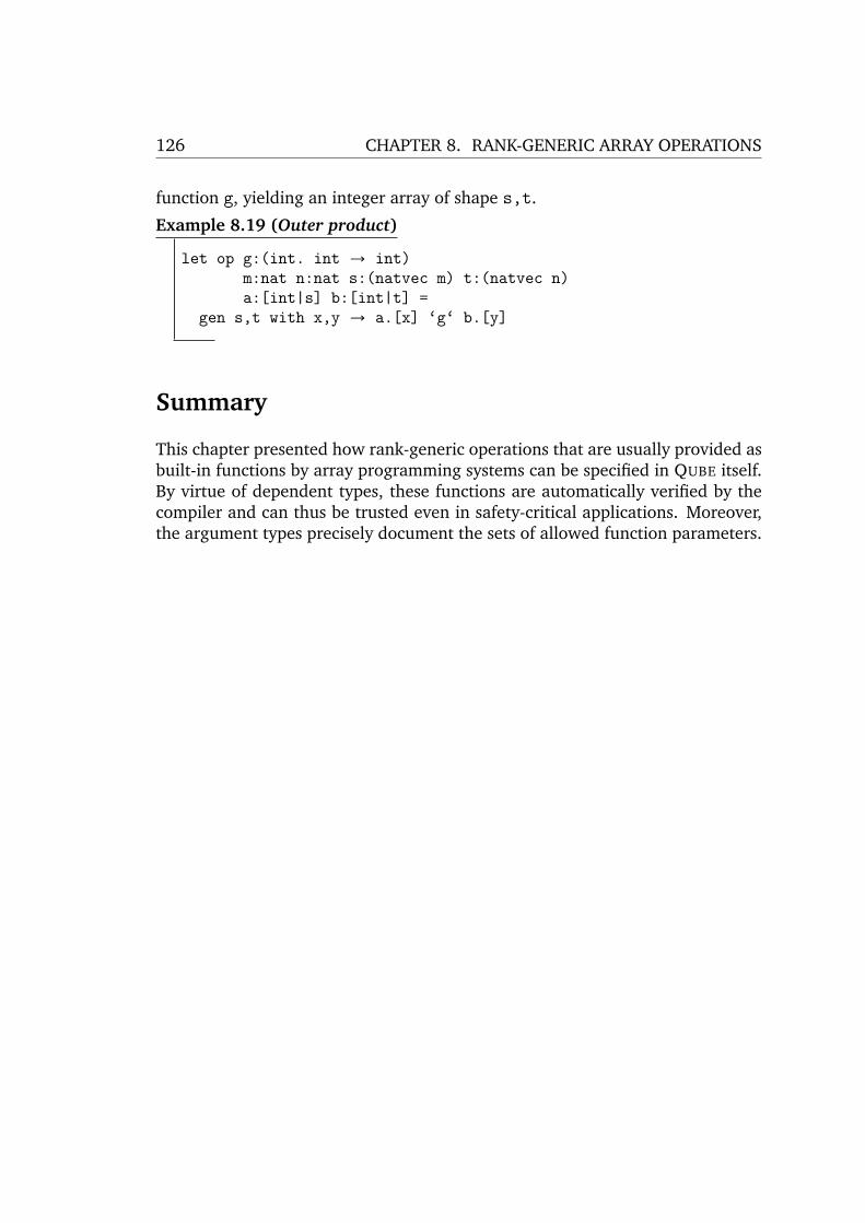
126 CHAPTER 8. RANK-GENERIC ARRAY OPERATIONS
function g, yielding an integer array of shape s,t.
Example 8.19 (Outer product)
let op g:(int. int → int)m:nat n:nat s:(natvec m) t:(natvec n)a:[int|s] b:[int|t] =
gen s,t with x,y → a.[x] ‘g‘ b.[y]
Summary
This chapter presented how rank-generic operations that are usually provided asbuilt-in functions by array programming systems can be specified in QUBE itself.By virtue of dependent types, these functions are automatically verified by thecompiler and can thus be trusted even in safety-critical applications. Moreover,the argument types precisely document the sets of allowed function parameters.

9Evaluation
This chapter evaluates the suitability of QUBE for practical program developmentby considering a number of example programs. The programs chosen are allwell-known and nicely demonstrate QUBE language features. Ideally, the eval-uation provides insights that motivate potential future extensions of the QUBE
language and compiler.All measurements were performed on an Apple iMac with a 2.8 GHz Core 2Duo processor and 4 GB RAM. The QUBE compiler uses LLVM version 2.8 as thebackend compiler. The reference C programs were compiled with GCC version4.2.1.The remainder of this chapter is structured as follows: Section 9.1 and Sec-tion 9.2 compare the efficiency of rank-generic implementations of the innerproduct and the convolution with C implementations of the algorithms. Sec-tion 9.3 investigates a QUBE implementation of Quicksort that makes use of de-structive array updates to achieve better run-time performance.
9.1 Matrix Multiplication and Inner Product
Matrix multiplication is an important operation in linear algebra. The innerproduct generalises matrix multiplication to arrays of arbitrary rank. As a firstmicro-benchmark, this section compares the rank-generic inner product with anaive (but reasonable) implementation of matrix multiplication in C.
127
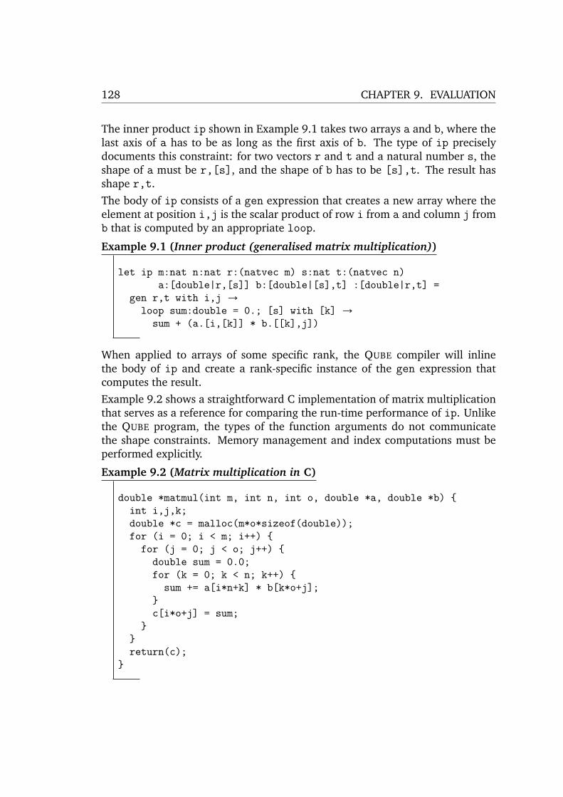
128 CHAPTER 9. EVALUATION
The inner product ip shown in Example 9.1 takes two arrays a and b, where thelast axis of a has to be as long as the first axis of b. The type of ip preciselydocuments this constraint: for two vectors r and t and a natural number s, theshape of a must be r,[s], and the shape of b has to be [s],t. The result hasshape r,t.The body of ip consists of a gen expression that creates a new array where theelement at position i,j is the scalar product of row i from a and column j fromb that is computed by an appropriate loop.
Example 9.1 (Inner product (generalised matrix multiplication))
let ip m:nat n:nat r:(natvec m) s:nat t:(natvec n)a:[double|r,[s]] b:[double|[s],t] :[double|r,t] =
gen r,t with i,j →loop sum:double = 0.; [s] with [k] →
sum + (a.[i,[k]] * b.[[k],j])
When applied to arrays of some specific rank, the QUBE compiler will inlinethe body of ip and create a rank-specific instance of the gen expression thatcomputes the result.Example 9.2 shows a straightforward C implementation of matrix multiplicationthat serves as a reference for comparing the run-time performance of ip. Unlikethe QUBE program, the types of the function arguments do not communicatethe shape constraints. Memory management and index computations must beperformed explicitly.
Example 9.2 (Matrix multiplication in C)
double *matmul(int m, int n, int o, double *a, double *b) {int i,j,k;double *c = malloc(m*o*sizeof(double));for (i = 0; i < m; i++) {
for (j = 0; j < o; j++) {double sum = 0.0;for (k = 0; k < n; k++) {
sum += a[i*n+k] * b[k*o+j];}c[i*o+j] = sum;
}}return(c);
}

9.2. RANK-GENERIC CONVOLUTION 129
Figure 9.1 compares the run-times of the rank-generic inner product, a rank-specific instance of the inner product and the C matrix multiplication when ap-plied to arrays of shape [1024,1024].
0s
2s
4s
6s
8s
10s
QUBE: ip QUBE: matmul C: matmul
6.9s 6.5s5.6s
Figure 9.1: Run-times of inner product in QUBE, matrix multiplication in QUBE,and matrix multiplication in C for arrays of shape [1024,1024].
All programs perform roughly equally well. In particular, the rank-generic in-stance performs so well because the compiler’s index vector elimination can re-place the offset computations ι r i and ι t j with scalar indices such that neitherof the index vectors i and j manifests at run-time. The rank-specific QUBE pro-gram performs somewhat better because the function is inlined into the applyingcontext where all shapes are constants. Somewhat mysteriously, the C programperforms even better. We attribute these improvements to differences betweenthe gcc and LLVM optimisation and code generation schemes.
9.2 Rank-Generic Convolution
As a second micro-benchmark, this section investigates array convolution. Rank-generic convolution is a straightforward extension of the well-known convolu-tion on time-discrete 1D signals f and g of length m and n≤ m, respectively.
( f ∗ g)(i) =m∑
j=0
( f (i+ j) · g(m− j))
m−n+1
i=0
Example 9.3 shows a rank-generic convolution function written in QUBE. For anyrank r, the function takes a rank r array f of some shape fs and another rank r

130 CHAPTER 9. EVALUATION
array g of some other shape gs that must not exceed fs. First, g is reverted bymeans of the function reverse defined in Section 8.4. Then, a gen expressionmoves the resulting array g’ over all subarrays of f of shape gs. At each position,a loop computes the sum of the element-wise product of g’ and the underlyingsubarray.
Example 9.3 (Rank-generic convolution)
let convolve r:nat fs:(natvec r) f:[double|fs]gs:(natvec_le r fs) g:[double|gs] =
let g’ = reverse r gs g ingen vmap fs,gs (fsi,gsi → fsi-gsi+1) with x →
loop sum:double = 0.; gs with y →sum + f.[vmap x,y (xi,yi → xi+yi)] * g’.[y]
Again, we use a rank-specific C implementation of the algorithm as a referenceto evaluate the efficiency of convolve. Example 9.4 shows the correspondingC program that computes a 2D convolution. With four nested for-loops andextensive index computations, the program is substantially more complicatedthan the QUBE program.
Example 9.4 (2D Convolution in C)
double *convolve( int fm, int fn, double *f,int gm, int gn, double *g) {
int ri,rj,gi,gj;double *gr = reverse(gm,gn,g);int rm = fm-gm+1;int rn = fn-gn+1;double *r = malloc(rm*rn*sizeof(double));for (ri = 0; ri < rm; ri++) {
for (rj = 0; rj < rn; rj++) {double sum = 0.0;for (gi = 0; gi < gm; gi++) {
for (gj = 0; gj < gn; gj++) {sum += f[(ri+gi)*fn+rj+gj] * gr[gi*gn+gj];
}}r[ri*rn+rj] = sum;
}}free(gr);return(r);
}

9.2. RANK-GENERIC CONVOLUTION 131
Figure 9.2 compares the run-times of the rank-generic convolution, a rank-specificconvolution in QUBE, and the C program. All programs have been applied to anarray of shape [10240,10240] and a [3,3] filter kernel.
0s
2s
4s
6s
8s
10s
QUBE: RG Conv QUBE: 2D Conv C: 2D Conv
6.1s
0.5s 0.8s
Figure 9.2: Run-times of rank-generic convolution in QUBE, 2D convolution inQUBE, and 2D convolution in C for arrays of shape [10240,10240] and [3,3].
Almost eight times slower than the reference program, the rank-generic convo-lution turns out to be a stress-test for the language implementation for three rea-sons. First, since r is unknown, the gen and loop expressions cannot be mappedto finite nestings of for-loops. Instead, both expressions are implemented bymeans of recursive functions which causes some function call overhead. Sec-ond, although the compiler’s index vector elimination scheme simplifies the off-set computation ι fs (vmap x,y (xi,yi → xi+yi)) into (ι fs x)+(ι fs y),it cannot further simplify the two offset computations such that they have becomputed by means of separate for-loops. Third, as both index vectors x and yare required to determine the offset into f, memory for the two vectors must bedynamically allocated. Since the amount of work performed by each instance ofthe innermost loop is small, the memory management overhead is significant.
As a more positive result, the rank-specific instance of convolve, which is thetypical case, only consumes 63% of the time required by the reference program.One reason for the good performance is that none of the problems hamperingthe rank-generic program occurs in the rank-specific setting. Moreover, the QUBE
compiler inlines the definition of convolve into the applying context where theloop boundaries and array sizes are constants instead of variables that must bekept in registers.

132 CHAPTER 9. EVALUATION
9.3 Quicksort
Fig. 9.3 shows a type-safe implementation of Hoare’s quicksort algorithm forsorting integer arrays. The program aims to mimic the well-known imperativeimplementations of quicksort as closely as possible. To achieve good perfor-mance, the program makes extensive use of uniqueness types that allow for de-structive array updates.The type bounded l u describes all integers in the inclusive interval [l,u]. Theauxiliary function swap takes a unique array and destructively exchanges theelements at two given index positions i and j. The types of the indices ensurethat no out-of-bounds accesses can occur.The function qsort takes a unique array arr of length n and two integers land r that specify the indices of the leftmost and the rightmost array elementto be sorted. When there are at least two elements to be sorted, the programdetermines a pivot element and partitions the array such that all elements lessthan or equal to the pivot element are moved to its left and all other elementsare moved to its right. Both parts of the array are then sorted recursively. Theresult of qsort has polymorphic uniqueness, such that it may be used in placeswhere either a unique array or a shared array is expected.The partitioning function partition takes the unique array, the interval of el-ements to be sorted given by l and r and the initial position pivot_idx ofthe pivot element in the interval. The function swaps the pivot element to therightmost position in the interval. Thereafter, it uses the tail-recursive functionploop to rearrange the array elements. The function traverses the array with aread index read and swaps all elements less than or equal to the pivot elementsto a store index store that marks the boundary between both parts of the in-terval. At the end of the loop, the pivot element is swapped to the final indexstore. partition returns the partitioned array and the new location of thepivot element.The second function qsort is merely a wrapper function that parameterises therecursive quicksort function.Figure 9.4 compares the run-times of a QUBE implementation of quicksort witha corresponding reference implementation in C. As a worst-case input, both pro-grams are applied to arrays with ten million integers that are initially sorted inreverse order. The QUBE program takes 50% more time to sort the array thanthe C program. The overhead stems from the memory management required toallocate and garbage collect the tuples returned by partition. Since ploop isa tail-recursive function that has no further call-sites, the LLVM inlines the func-tion into the body of partition and subsequently converts the tail-recursioninto a loop.

9.3. QUICKSORT 133
type bounded l:int u:int = { v:int | l <= v & v <= u }
let swap n:nat arr:*[int|[n]] i:(index n) j:(index n) =let (arr,ai) = arr![[i]] inlet (arr,aj) = arr![[j]] inlet arr = arr![[i]] ← aj inlet arr = arr![[j]] ← ai inarr
let partition n:nat arr:*[int|[n]]l:nat r:{v:int|v<n} pivot_idx:(bounded l r) =
let (arr,pivot) = arr![[pivot_idx]] inlet arr = swap n arr pivot_idx r inlet rec ploop arr:*[int|[n]] read:(bounded l r)
store:(bounded l read) :*(?[int|[n]],bounded l r) =if read < rthen
let (arr,arr_read) = arr![[read]] inif arr_read <= pivotthen ploop (swap n arr read store) (read+1) (store+1)else ploop arr (read+1) store
else (swap n arr store r,store)inploop arr l l
let rec qsort n:nat arr:*[int|[n]] l:nat r:{v:int|v<n} :?[int|[n]] =if l < rthen
let pivot_idx = (l+r)/2 inlet (arr,pivot_idx) = partition n arr l r pivot_idx inlet arr = qsort n arr l (pivot_idx-1) inlet arr = qsort n arr (pivot_idx+1) r inarr
else arr
let qsort n:nat a:*[int|[n]] = qsort n a 0 (n-1)
Figure 9.3: Quicksort in QUBE

134 CHAPTER 9. EVALUATION
0.00s
0.25s
0.50s
0.75s
1.00s
QUBE: QSort C: QSort
0.75s
0.5s
Figure 9.4: Run-times of quicksort in QUBE and in C for ten million elements.
Summary
This chapter evaluated the suitability of the QUBE programming language and itsimplementation for actual program development by means of some well-knownexample programs.The rank-generic implementations of the inner product and the convolution areat the same time simpler and more powerful than the corresponding rank-specificC programs. In both cases, the dependent types are unobtrusive and naturallydocument the constraints the functions impose on the arguments. The QUBE im-plementation of quicksort uses uniqueness types and destructive array updates tomimic the well-known imperative implementations of the algorithm. The com-bination of dependent types and uniqueness types causes some notational over-head, in particular since the partitioning loop maps to a tail-recursive functionthat requires its own set of typed arguments.At least in a rank-specific context, which is the typical case, the run-time perfor-mance of the QUBE programs for inner product and convolution is on par withthe C functions. In the case of quicksort, we have identified tuple constructionas a source of overhead. An optimisation that replaces passing boxed tuples be-tween functions with passing the individual components could eliminate largeparts of this overhead.

10Conclusion and Future Work
Making the expressive power of dependent types available for practical programdevelopment is a subject of ongoing research. It is a particular challenge to de-sign programming systems with dependent types in a way such that the user isnot required to have expert knowledge in type theory. QUBE is a new program-ming language that employs dependent types in the context of array program-ming where their use is both intuitive and beneficial.Dependent types are intuitive for array programs because rank and shape areinherent properties of multidimensional arrays. Scientific programmers are usedto specifying their algorithms in terms of array shapes: each undergraduatecourse on linear algebra teaches the function type of matrix multiplication asRm×n ×Rn×p → Rm×p. Dependent types allow the developer to concisely expressthe constraints on the array shapes.Dependent types are beneficial for array programs because base type errors, rankerrors, shape errors, and even array boundary violations can be statically ruledout. Array programs with dependent types are thus correct by construction.Since static verification makes dynamic checks such as array bounds checks ob-solete, dependent types also help to improve the run-time efficiency of arrayprograms.The syntax, semantics, and type system of QUBE have been formalised by meansof the core language QUBECORE that captures the essential concepts of QUBE with-out any syntactic sugar. Multidimensional array types are parameterised by in-teger vectors that represent the array shape. Integer vector types are in turn
135

136 CHAPTER 10. CONCLUSION AND FUTURE WORK
parameterised by integers that represent the vector length. As a significant re-sult of this thesis, the type system of QUBECORE has a formal correctness proof,i. e., a proof that well-typed expressions cannot exhibit any run-time errors.Based on QUBECORE, the actual QUBE programming language adds a host of fea-tures to facilitate practical programming, such as an ML-style module systemand support for stateful computations. QUBE is implemented by a compiler thattranslates programs into efficient native code. In order to decide whether twodependent types are equivalent or in a subtype relation, the compiler performstype checking in collaboration with a theorem prover for the Satisfiability Mod-ulo Theories problem of first-order logic. Since SMT solving proceeds fully au-tomatically, the QUBE type checker behaves very much like a (very powerful)type checker for a mainstream programming language that either accepts or re-jects a program without further interaction with the user. Moreover, the QUBE
compiler uses the rank and shape information from the dependent types to in-strument programs with corresponding expressions wherever these propertiesare required at run-time, for example to compute memory offsets. The benefitsof this strategy are twofold: First, once the structural properties of arrays areencoded explicitly in the intermediate program, they become subject to compileroptimisation. Second, multidimensional arrays may be represented as mere se-quences of data without additional shape descriptors or type tags. In effect, thecompiled programs contain very little overhead.Unlike interpreted languages, QUBE does not provide a large number of built-inarray operations. Instead, the standard array operations can be defined in QUBE
itself by means of the versatile gen and loop expressions. Due to static typing,these array operations are inherently type-safe. QUBE appears to be well-suitedfor developing practical array programs. For most rank-generic functions, depen-dent types are unobtrusive as they naturally express the constraints a functionimposes on its arguments. For the programs investigated, the run-time perfor-mance of QUBE programs is roughly on par with corresponding C programs.The development of QUBE has focused on static verification of rank-generic arrayprograms. There are several potential directions for future extensions of both thelanguage and the compiler.The most glaring omission in QUBE’s type system is missing support for poly-morphism. In the current system, functions must be re-implemented for eachargument type. Adding support for parametric polymorphism would allow theuser to define functions that operate on values of arbitrary types.Furthermore, the QUBE compiler would greatly benefit from additional programoptimisation schemes. QUBE encourages a programming style where programsare composed from predefined rank-generic array operations. Although elegant,the resulting code is plagued with excessive creation of temporary arrays that

137
increase both the program’s time and memory demands. In order to avoidtemporary arrays, QUBE could employ similar techniques as the SAC compiler.WITH-LOOP-FOLDING [88] is an effective deforestation technique that replacesselections into arrays with the selected element’s definition. In QUBE, it shouldbe possible to perform deforestation even in a rank-generic setting by using theSMT solver to determine the code that defines a given element.Finally, due to its functional and side-effect free semantics and its focus on arrayoperations that uniformly apply to a large number of elements, QUBE lends it-self well for non-sequential evaluation on multi-core processors or even general-purpose graphics processing units. Since almost all array operations are definedin terms of gen and loop expressions, the implementation efforts can be concen-trated on these expressions. The evaluation of gen can be trivially distributedover multiple worker threads. In contrast, the accumulator variable and the de-terministic evaluation order of loop preclude a naive approach to concurrentevaluation. Again, taking a leaf out of SAC’s book, a potential remedy could beto define a parallel loop that does not guarantee a certain evaluation orderand uses an additional function to combine the partial results.The current QUBE compiler may be used as a basis to explore all the directionsof future work outlined above.

138 CHAPTER 10. CONCLUSION AND FUTURE WORK

Bibliography
[1] Alfred V. Aho, Ravi Sethi, and Jeffrey D. Ullman. Compilers: Principles,Techniques, and Tools. Addison Wesley, Reading, Massachusetts, USA,1986.
[2] Thorsten Altenkirch, Conor McBride, and James McKinna. Why DependentTypes Matter. Manuscript, available online, April 2005.
[3] Andrew W. Appel. SSA is Functional Programming. ACM SIGPLAN No-tices, vol. 33(4), pp. 17–20, 1998.
[4] Lennart Augustsson. Cayenne – A Language with Dependent Types. In Pro-ceedings of the third ACM SIGPLAN International Conference on Func-tional Programming, ICFP ’98, pp. 239–250. ACM Press, New York, NY,USA, 1998.
[5] Henk Barendregt. The Lambda Calculus: Its Syntax and Semantics, vol. 103of Studies in Logics and the Foundations of Mathematics. North Holland,Amsterdam, The Netherlands, 1981.
[6] Henk Barendregt. Introduction to Generalized Type Systems. Journal ofFunctional Programming, vol. 1(2), pp. 125–154, 1991.
[7] Henk Barendregt. Lambda Calculi with Types, vol. 2 of Handbook of Logicin Computer Science, pp. 117–309. Oxford University Press, Inc. NewYork, NY, USA, 1992.
[8] Henk Barendregt and Erik Barendsen. Introduction to Lambda Calculus.Technical report, Department of Computer Science, Catholic University ofNijmegen, 1991.
[9] Erik Barendsen and Sjaak Smetsers. Conventional and Uniqueness Typ-ing in Graph Rewrite Systems. In Rashmi K. Shyamasundar, editor, Foun-dations of Software Technology and Theoretical Computer Science, 13thConference, FSTTCS’93, Lecture Notes in Computer Science, vol. 761, pp.41–51. Springer Verlag, Berlin, Germany, 1993.
139

140 BIBLIOGRAPHY
[10] Robert Bernecky. Compiling APL. In Lenore M. Restifo Mullin et. al.,editor, Arrays, Functional Languages, and Parallel Systems, pp. 19–33.Kluwer Academic Publishers, 1991.
[11] Robert Bernecky. An Overview of the APEX Compiler. Technical Report305/97, University of Toronto, Toronto, Canada, 1997.
[12] Robert Bernecky, Stephan Herhut, Sven-Bodo Scholz, Kai Trojahner,Clemens Grelck, and Alex Shafarenko. Index Vector Elimination: Mak-ing Index Vectors Affordable. In Zoltán Horváth and Viktória Zsók, editors,Proceedings of the 18th International Symposium on Implementation andApplication of Functional Languages, IFL’06, Technical Report, vol. 2006-S01. Eötvös Loránd University, Faculty of Informatics, Budapest, Hungary,2006.
[13] Richard S. Bird. An Introduction to Functional Programming using Haskell.Series in Computer Science. Prentice Hall Europe, London, UK, secondedition, 1998.
[14] Guy E. Blelloch. Programming Parallel Algorithms. Communications ofthe ACM, vol. 39(3), pp. 85–97, 1996.
[15] Johannes Blume. A Decision Procedure for Linear Vector Arithmetic. Bach-elor’s thesis, Institut für Softwaretechnik und Programmiersprachen, Uni-versität zu Lübeck, Lübeck, 2008.
[16] Hans Boehm, Alan Demers, and Scott Shenker. Mostly Parallel GarbageCollection. In Proceedings of the ACM SIGPLAN 1991 Conference on Pro-gramming Languages Design and Implementation, PLDI ’91, ACM SIG-PLAN Notices, vol. 26, pp. 157–164. ACM Press, New York, NY, USA,1991.
[17] Aaron R. Bradley and Zohar Manna. The Calculus of Computation.Springer-Verlag, Berlin, Heidelberg, Germany, 2007.
[18] Aaron R. Bradley, Zohar Manna, and Henny B. Sipma. What’s DecidableAbout Arrays? In E. Allen Emerson and Kedar S. Namjoshi, editors, Ver-ification, Model Checking, and Abstract Interpretation, 7th InternationalConference, VMCAI 2006, Lecture Notes in Computer Science, vol. 3855,pp. 427–442. Springer-Verlag, Berlin, Heidelberg, Germany, 2006.
[19] Florian Büther. A Compiler for Qube, a Functional Array Programming Lan-guage with Dependent Types. Studienarbeit, Institut für Softwaretechnikund Programmiersprachen, Universität zu Lübeck, Lübeck, 2008.

BIBLIOGRAPHY 141
[20] Florian Büther. Modules and State for the Functional Programming Lan-guage Qube. Diploma thesis, Institut für Softwaretechnik und Program-miersprachen, Universität zu Lübeck, Lübeck, 2010.
[21] David Cann. Retire Fortran? A Debate Rekindled. Communications of theACM, vol. 35(8), pp. 81–89, 1992.
[22] Emmanuel Chailloux, Pascal Manoury, and Bruno Pagano. Developing Ap-plications with Objective Caml, 2000.
[23] Manuel M. T. Chakravarty, Roman Leshchinskiy, Simon L. Peyton Jones,Gabriele Keller, and Simon Marlow. Data Parallel Haskell: a Status Report.In Proceedings of the 2007 Workshop on Declarative Aspects of MulticoreProgramming, DAMP ’07, pp. 10–18. ACM Press, New York, NY, USA,2007.
[24] Manuel M.T. Chakravarty and Gabriele Keller. An Approach to Fast Arraysin Haskell. In Johan Jeuring and Simon L. Peyton Jones, editors, AdvancedFunctional Programming, 4th International School, AFP 2002, LectureNotes in Computer Science, vol. 2638, pp. 27–58. Springer-Verlag, Berlin,Heidelberg, Germany, 2003.
[25] Bradford L. Chamberlain, Sung-Eun Choi, Steven J. Deitz, and LawrenceSnyder. The High-Level Parallel Language ZPL Improves Productivity andPerformance. In Proceedings of the First Workshop on Productivity andPerformance in High-End Computing (PPHEC-04), pp. 66–75, 2004.
[26] Alonzo Church. The Calculi of Lambda Conversion. Princeton UniversityPress, Princeton, NJ, USA, 1941.
[27] Stephen A. Cook. The Complexity of Theorem-Proving Procedures. In Pro-ceedings of the Third Annual ACM Symposium on Theory of Computing,STOC ’71, pp. 151–158. ACM Press, New York, NY, USA, 1971.
[28] Martin Davis, George Logemann, and Donald Loveland. A Machine Pro-gram for Theorem-Proving. Communications of the ACM, vol. 5(7), pp.394–397, 1962.
[29] Martin Davis and Hilary Putnam. A Computing Procedure for Quantifica-tion Theory. Journal of the ACM, vol. 7(3), pp. 201–215, 1960.
[30] Leonardo M. de Moura and Nikolaj Bjørner. Z3: An Efficient SMT Solver.In C.R. Ramakrishnan and Jakob Rehof, editors, Tools and Algorithms forthe Construction and Analysis of Systems, 14th International Conference,

142 BIBLIOGRAPHY
TACAS’08, Lecture Notes in Computer Science, vol. 4963, pp. 337–340.Springer-Verlag, Berlin, Heidelberg, Germany, 2008.
[31] Luiz de Rose and David Padua. Techniques for the Translation of MATLABPrograms into Fortran 90. ACM Transactions on Programming Languagesand Systems, vol. 21(2), pp. 286–323, 1999.
[32] Edsko de Vries, Rinus Plasmeijer, and David M. Abrahamson. UniquenessTyping Simplified. In Olaf Chitil, Zoltán Horváth, and Viktória Zsók, edi-tors, Implementation and Application of Functional Languages, 19th In-ternational Symposium, IFL’07, Lecture Notes in Computer Science, vol.5083, pp. 201 – 218. Springer-Verlag, Berlin, Heidelberg, Germany, 2008.
[33] Bruno Dutertre and Leonardo M. de Moura. A Fast Linear-ArithmeticSolver for DPLL(T). In Thomas Ball and Robert B. Jones, editors, Com-puter Aided Verification, 18th International Conference, CAV 2006, Lec-ture Notes in Computer Science, vol. 4144, pp. 81–94. Springer Verlag,Heidelberg, Germany, 2006.
[34] Niklas Eén and Niklas Sörensson. An Extensible SAT-solver. In EnricoGiunchiglia and Armando Tacchella, editors, SAT ’03, Lecture Notes inComputer Science, vol. 2919, pp. 502–518. Springer-Verlag, Berlin, Hei-delberg, Germany, 2003.
[35] Adin D. Falkoff and Kenneth E. Iverson. The Design of APL. IBM Journalof Research and Development, vol. 17(4), pp. 324–334, 1973.
[36] Cormac Flanagan. Hybrid Type Checking. In Conference Record of the33rd ACM SIGPLAN-SIGACT Symposium on Principles of ProgrammingLanguages, POPL ’06, pp. 245–256. ACM Press, New York, NY, USA, 2006.
[37] Cormac Flanagan, Amr Sabry, Bruce F. Duba, and Matthias Felleisen. TheEssence of Compiling with Continuations. In Proceedings of the ACM SIG-PLAN 1993 Conference on Programming Language Design and Implemen-tation, PLDI ’93, pp. 237–247. ACM Press, New York, NY, USA, 1993.
[38] Anwar Ghuloum, Terry Smith, Gansha Wu, Xin Zhou, Jesse Fang, PengGuo, Byoungro So, Mohan Rajagopalan, Yongjian Chen, and Biao Chen.Future-Proof Data Parallel Algorithms and Software on Intel Multi-Core Ar-chitecture. Intel Technology Journal, vol. 11(4), pp. 333–346, 2007.
[39] Clemens Grelck. Shared Memory Multiprocessor Support for FunctionalArray Processing in SAC. Journal of Functional Programming, vol. 15(3),pp. 353–401, 2005.

BIBLIOGRAPHY 143
[40] Clemens Grelck, Karsten Hinckfuß, and Sven-Bodo Scholz. With-Loop Fu-sion for Data Locality and Parallelism. In Andrew Butterfield, ClemensGrelck, and Frank Huch, editors, Implementation and Application ofFunctional Languages, 17th International Workshop, IFL’05, LectureNotes in Computer Science, vol. 4015, pp. 178–195. Springer-Verlag,Berlin, Heidelberg, Germany, 2006.
[41] Clemens Grelck, Frank Penczek, and Kai Trojahner. CAOS: A Domain-Specific Language for the Parallel Simulation of Cellular Automata. In Vik-tor Malyshkin, editor, Parallel Computing Technologies, 9th InternationalConference, PaCT’07, Lecture Notes in Computer Science, vol. 4671, pp.410–417. Springer-Verlag, Berlin, Heidelberg, Germany, 2007.
[42] Clemens Grelck and Sven-Bodo Scholz. SAC: A Functional Array Languagefor Efficient Multithreaded Execution. International Journal of Parallel Pro-gramming, vol. 34(4), pp. 383–427, 2006.
[43] Clemens Grelck, Sven-Bodo Scholz, and Alex Shafarenko. A BindingScope Analysis for Generic Programs on Arrays. In Andrew Butterfield,Clemens Grelck, and Frank Huch, editors, Implementation and Applica-tion of Functional Languages, 17th International Workshop, IFL’05, Lec-ture Notes in Computer Science, vol. 4015, pp. 212–230. Springer-Verlag,Berlin, Heidelberg, Germany, 2006.
[44] Clemens Grelck, Sven-Bodo Scholz, and Kai Trojahner. With-Loop Scalar-ization: Merging Nested Array Operations. In Philip W. Trinder, GregMichaelson, and Ricardo Pena, editors, mplementation of Functional Lan-guages, 15th International Workshop, IFL’03, Lecture Notes in ComputerScience, vol. 3145, pp. 118–134. Springer-Verlag, Berlin, Heidelberg, Ger-many, 2004.
[45] Clemens Grelck and Kai Trojahner. Implicit Memory Management for SAC.In Clemens Grelck and Frank Huch, editors, Implementation and Applica-tion of Functional Languages: 16th International Workshop, IFL’04, Tech-nical Report, vol. 0408, pp. 335–348. University of Kiel, 2004.
[46] Clemens Grelck, Tim van Deurzen, Stephan Herhut, and Sven-BodoScholz. An Adaptive Compilation Framework for Generic Data-Parallel Ar-ray Programming. In Andreas Krall and Gergö Barany, editors, 15th Work-shop on Compilers for Parallel Computing, CPC’10. Institute of ComputerLanguages, Vienna University of Technology, Vienna, Austria, 2010.

144 BIBLIOGRAPHY
[47] Dick Grune, Henri E. Bal, Ceriel J. H. Jacobs, and Koen G. Langendoen.Modern Compiler Design. John Wiley & Sons, West Sussex, England, 2000.
[48] Kurt Gödel. Über formal unentscheidbare Sätze der Principia Mathematicaund verwandter Systeme. Monatshefte für Mathematik und Physik, vol. 38,pp. 173–198, 1931.
[49] Robert Harper. Introduction to Standard ML. Carnegie Mellon University,Pittsburgh, Pennsylvania, USA, 1993.
[50] John R. Harrison. Handbook of Practical Logic and Automated Reasoning.Cambridge University Press, 2009.
[51] Stephan Herhut, Sven-Bodo Scholz, Robert Bernecky, Clemens Grelck,and Kai Trojahner. From Contracts Towards Dependent Types: Proofs by Par-tial Evaluation. In Olaf Chitil, Zoltan Horváth, and Viktória Zsók, editors,Implementation and Application of Functional Languages: 19th Interna-tional Workshop, IFL’07, Lecture Notes in Computer Science, vol. 5083,pp. 254–273. Springer-Verlag, Berlin, Heidelberg, Germany, 2008.
[52] J. Roger Hindley and Jonathan P. Seldin. Introduction to Combinators andLambda Calculus. London Mathematical Society Student Texts. CambridgeUniversity Press, Cambridge, UK, 1986.
[53] Paul Hudak and Adrienne Bloss. The Aggregate Update Problem in Func-tional Programming Systems. In Proceedings of the 12th ACM SIGACT-SIGPLAN symposium on Principles of programming languages, POPL’85,pp. 300–313. ACM Press, New York, NY, USA, 1985.
[54] Paul Hudak, Simon L. Peyton Jones, Philip Wadler, et al. Report on theProgramming Language Haskell, A Non-strict, Purely Functional Language.SIGPLAN Notices, vol. 27(5), 1992.
[55] Kenneth E. Iverson. A Programming Language. John Wiley, New York, NY,USA, 1962.
[56] Kenneth E. Iverson. Programming in J. Iverson Software Inc., Toronto,Canada, 1991.
[57] Kenneth E. Iverson. J Introduction and Dictionary. Iverson Software Inc.,Toronto, Canada, 1995.
[58] C. Barry Jay. The FISh Language Definition. Technical report, School ofComputing Sciences, University of Technology, Sidney, Australia, 1998.

BIBLIOGRAPHY 145
[59] C. Barry Jay and Paul A. Steckler. The Functional Imperative: Shape! InChris Hankin, editor, Proceedings of the 7th European Symposium onProgramming, ESOP’98, Held as Part of the Joint European Conferenceon Theory and Practice of Software, ETAPS’98, Lecture Notes in Com-puter Science, vol. 1381, pp. 139–53. Springer-Verlag, Berlin, Heidelberg,Germany, 1998.
[60] Thomas Johnsson. Lambda Lifting: Transforming Programs to RecursiveEquations. In Proceedings 1985 Conference on Functional ProgrammingLanguages and Computer Architecture, Lecture Notes in Computer Sci-ence, vol. 201. Springer-Verlag, Berlin, Heidelberg, Germany, 1985.
[61] Pramod G. Joisha and Prithviraj Banerjee. An Algebraic Array Shape Infer-ence System for MATLAB. ACM Transactions on Programming Languagesand Systems, vol. 28(5), pp. 848–907, 2006.
[62] Guy L. Steele Jr. Debunking the “Expensive Procedure Call” Myth, or Proce-dure Call Implementations Considered Harmful, or LAMBDA: The UltimateGOTO. In Proceedings of the 1977 Annual Conference, ACM’77, pp. 153–162. ACM Press, New York, NY, USA, 1977.
[63] Gabriele Keller, Manuel M.T. Chakravarty, Roman Leshchinskiy, Si-mon Peyton Jones, and Ben Lippmeier. Regular, Shape-Polymorphic, Par-allel Arrays in Haskell. In Proceedings of the 15th ACM SIGPLAN Inter-national Conference on Functional Programming, ICFP’10, pp. 261–272.ACM Press, New York, NY, USA, 2010.
[64] Werner Kluge. Abstract Computing Machines: A Lambda Calculus Perspec-tive. Springer-Verlag Berlin Heidelberg, 2005.
[65] Dietmar Kreye. A Compilation Scheme for a Hierarchy of Array Types. InThomas Arts and Markus Mohnen, editors, Implementation of FunctionalLanguages, 13th International Workshop, IFL’02, Lecture Notes in Com-puter Science, vol. 2312, pp. 18–35. Springer-Verlag, Berlin, Heidelberg,Germany, 2002.
[66] Daniel Kroening and Ofer Strichman. Decision Procedures. Springer-Verlag, Berlin, Heidelberg, 2008.
[67] Peter J. Landin. The Mechanical Evaluation of Expressions. Computer Jour-nal, vol. 6(4), pp. 308–320, 1964.

146 BIBLIOGRAPHY
[68] Chris Lattner. LLVM: An Infrastructure for Multi-Stage Optimization. Mas-ter’s thesis, Computer Science Dept., University of Illinois at Urbana-Champaign, Urbana, IL, Dec 2002.
[69] Xavier Leroy. The Objective Caml System release 3.11. INRIA, Rocquen-court, France, 2008.
[70] David MacQueen, Robert Harper, Robin Milner, et al. Functional Pro-gramming in ML. LFCS education, University of Edinburgh, Edinburgh,Scotland, UK, 1987.
[71] Simon Marlow and Simon Peyton Jones. Making a Fast Curry: Push/En-ter vs. Eval/Apply for Higher-Order Languages. In ICFP ’04: Proceedingsof the Ninth ACM SIGPLAN International Conference on Functional Pro-gramming, pp. 4–15. ACM Press, New York, NY, USA, 2004.
[72] Per Martin-Löf. Intuitionistic Type Theory. Bibliopolis, 1984.
[73] Conor McBride and James McKinna. The View from the Left. Journal ofFunctional Programming, vol. 14(1), pp. 69–111, January 2004.
[74] Cheryl McCosh. Type-Based Specialization in a Telescoping Compiler forMATLAB. Master Thesis TR03-412, Rice University, Houston, Texas, USA,2003.
[75] Robin Milner, Mads Tofte, and Robert Harper. The Definition of StandardML. MIT Press, Cambridge, Massachusetts, USA, 1990.
[76] Cleve Moler, John Little, and Steve Bangert. Pro-Matlab User’s Guide. TheMathWorks, Cochituate Place, 24 Prime Park Way, Natick, MA, USA, 1987.
[77] Matthew W. Moskewicz, Conor F. Madigan, Ying Zhao, Lintao Zhang, andSharad Malik. Chaff: Engineering an Efficient SAT Solver. In Proceedingsof the 38th Annual Design Automation Conference, DAC’01, pp. 530–535.ACM Press, New York, NY, USA, 2001.
[78] Greg Nelson and Derek C. Oppen. Simplification by Cooperating DecisionProcedures. ACM Transactions on Programming Languages and Systems,vol. 1(2), pp. 245–257, 1979.
[79] Derek C. Oppen. Complexity, Convexity and Combinations of Theories. The-oretical Computer Science, vol. 12(3), pp. 291 – 302, 1980.

BIBLIOGRAPHY 147
[80] Simon L. Peyton Jones. The Implementation of Functional ProgrammingLanguages. Series in Computer Science. Prentice-Hall, Englewood Cliffs,NJ, USA, 1987.
[81] Simon L. Peyton Jones. Haskell 98 Language and Libraries. CambridgeUniversity Press, Cambridge, UK, 2003.
[82] Benjamin C. Pierce. Types and Programming Languages. MIT Press, Cam-bridge, MA, USA, 2002.
[83] Benjamin C. Pierce. Advanced Topics in Types and Programming Languages.MIT Press, Cambridge, MA, USA, 2004.
[84] Marinus J. Plasmeijer and Marko van Eekelen. Concurrent Clean 2.0 Lan-guage Report. University of Nijmegen, The Netherlands, 2001.
[85] Mojzesz Presburger. Über die Vollständigkeit eines gewissen Systems derArithmetik ganzer Zahlen, in welchem die Addition als einzige Operationhervortritt. Comptes Rendus du I congrès de Mathématiciens des PaysSlaves, Warszawa, vol. , pp. 92–101, 1929.
[86] Patrick M. Rondon, Ming Kawaguchi, and Ranjit Jhala. Liquid Types. InProceedings of the ACM SIGPLAN 2008 Conference on Programming Lan-guage Design and Implementation, PLDI’08, SIGPLAN Notices, vol. 43(6),pp. 159–169. ACM Press, New York, NY, USA, 2008.
[87] Patrick M. Rondon, Ming Kawaguchi, and Ranjit Jhala. Liquid Types. CSETechreport, University of California, San Diego, California, USA, 2008.
[88] Sven-Bodo Scholz. With-loop-folding in SAC — Condensing Consecutive Ar-ray Operations. In Chris Clack, Tony Davie, and Kevin Hammond, editors,Selected Papers from the 9th International Workshop on Implementationof Functional Languages, IFL’97, Lecture Notes in Computer Science, vol.1467, pp. 72–92. Springer-Verlag, Berlin, Heidelberg, Germany, 1998.
[89] Sven-Bodo Scholz. Single Assignment C — Efficient Support for High-LevelArray Operations in a Functional Setting. Journal of Functional Program-ming, vol. 13(6), pp. 1005–1059, 2003.
[90] Sven-Bodo Scholz, Stephan Herhut, Clemens Grelck, and Frank Penczek.SAC 1.0 – Single Assignment C – Tutorial. Technical Report 498, School ofComputer Science, University of Hertfordshire, Hatfield, United Kingdom,2010.

148 BIBLIOGRAPHY
[91] Peter Sestoft. Demonstrating Lambda Calculus Reduction. In Torben Mo-gensen, David Schmidt, and I. Hal Sudburough, editors, The Essence ofComputation: Complexity, Analysis, Transformation. Essays Dedicated toNeil D. Jones, Lecture Notes in Computer Science, vol. 2566, pp. 420–435. Springer-Verlag, Berlin, Heidelberg, Germany, 2002.
[92] Jan Smith, Bengt Nordström, and Kent Petersson. Programming in Martin-Löf ’s Type Theory. Oxford University Press, 1990.
[93] Herb Sutter. A Fundamental Turn Toward Concurrency in Software. Dr.Dobb’s Journal, vol. 30(3), pp. 16–23, 2005.
[94] Kai Trojahner. Implicit Memory Management for a Functional Array Pro-cessing Language. Diploma thesis, Institut für Softwaretechnik und Pro-grammiersprachen, Universiät zu Lübeck, Lübeck, Germany, 2005.
[95] Kai Trojahner. Assembling Concurrent Programs Correctly from Data-Parallel Program Bricks. In Viktor Malyshkin, editor, Parallel ComputingTechnologies, 9th International Conference, PaCT’07, Lecture Notes inComputer Science, vol. 4671, pp. 410–417. Springer-Verlag, Berlin, Hei-delberg, Germany, 2007.
[96] Kai Trojahner and Clemens Grelck. Dependently Typed Array ProgramsDon’t Go Wrong. Journal of Logic and Algebraic Programming, vol. 78(7),pp. 643–664, 2009. The 19th Nordic Workshop on Programming Theory(NWPT 2007).
[97] Kai Trojahner and Clemens Grelck. Descriptor-Free Representation of Ar-rays with Dependent Types. In Sven-Bodo Scholz and Olaf Chitil, editors,Implementation and Application of Functional Languages, 20th interna-tional symposium, IFL’08, Lecture Notes in Computer Science, vol. 5836.Springer-Verlag, Berlin, Heidelberg, Germany, 2010.
[98] Kai Trojahner, Clemens Grelck, and Sven-Bodo Scholz. On OptimisingShape-Generic Array Programs using Symbolic Structural Information. InZoltán Horváth and Viktória Zsók, editors, Implementation and Appli-cation of Functional Languages, 18th International Symposium, IFL’06,Lecture Notes in Computer Science, vol. 4449, pp. 1–18. Springer-Verlag,Berlin, Heidelberg, Germany, 2007.
[99] Markus Weigel. Facilitating Array Programming with Dependent Types –Precise Error Messages and Implicit Index Arguments for Qube. Master’s the-sis, Institut für Softwaretechnik und Programmiersprachen, Universität zuLübeck, Lübeck, Germany, 2008.

BIBLIOGRAPHY 149
[100] Hongwei Xi. Applied Type System (extended abstract). In S. Baradi,M. Coppo, and F. Damiani, editors, Types for Proofs and Programs, ThirdInternational Workshop, TYPES’03, Lecture Notes in Computer Science,vol. 3085, pp. 394–408. Springer Verlag, Berlin, Germany, 2004.
[101] Hongwei Xi and Frank Pfenning. Eliminating Array Bound Checkingthrough Dependent Types. In Proceedings of ACM SIGPLAN Conferenceon Programming Language Design and Implementation, PLDI’98, ACMSIGPLAN Notices, vol. 33(5), pp. 249–257. ACM Press, New York, NY,USA, 1998.
[102] Hongwei Xi and Frank Pfenning. Dependent Types in Practical Program-ming. In Alexander Aiken, editor, Proceedings of the 26th ACM SIGPLAN-SIGACT symposium on Principles of programming languages, POPL’99,pp. 214–227. ACM Press, New York, NY, USA, 1999.
[103] Christoph Zenger. Indexed Types. Theorectical Computer Science, vol.187(1-2), pp. 147–165, 1997.