Quaternary Science Reviews · (sea-levelequivalent,SLE)(Table1);thisisapproximatelytwicethe size of...
28
Invited review Differences between the last two glacial maxima and implications for ice-sheet, d 18 O, and sea-level reconstructions Eelco J. Rohling a, b, *, 1 , Fiona D. Hibbert a, 1 , Felicity H. Williams a, b, 1 , Katharine M. Grant a , Gianluca Marino a , Gavin L. Foster b , Rick Hennekam c, d , Gert J. de Lange d , Andrew P. Roberts a , Jimin Yu a , Jody M. Webster e , Yusuke Yokoyama f, g, h a Research School of Earth Sciences, The Australian National University, Canberra, ACT 2601, Australia b Ocean and Earth Science, University of Southampton, National Oceanography Centre, Southampton SO14 3ZH, UK c Department of Ocean Systems, Royal Netherlands Institute for Sea Research (NIOZ), Utrecht University, PO Box 59,1790 AB Den Burg, Texel, The Netherlands d Department of Earth Sciences-Geochemistry, Faculty of Geosciences, Utrecht University, Utrecht, The Netherlands e School of Geosciences, The University of Sydney, NSW 2006, Australia f Atmosphere and Ocean Research Institute, The University of Tokyo, 5-1-5 Kashiwanoha, Chiba 277-8564, Japan g Department of Earth and Planetary Science, Graduate School of Science, The University of Tokyo, 7-3-1 Hongo, Bunkyoku, Tokyo 113-0033, Japan h Department of Biogeochemistry, Japan Agency for Marine-Earth Science and Technology, 2-15 Natsushimacho, Yokosuka 237-0061, Japan article info Article history: Received 8 May 2017 Received in revised form 31 August 2017 Accepted 20 September 2017 Available online 10 October 2017 Keywords: Last Glacial Maximum Penultimate Glacial Maximum Sea level Ice volume d 18 O Arctic ice shelf Last Interglacial Glacioisostatic adjustment abstract Studies of past glacial cycles yield critical information about climate and sea-level (ice-volume) vari- ability, including the sensitivity of climate to radiative change, and impacts of crustal rebound on sea- level reconstructions for past interglacials. Here we identify significant differences between the last and penultimate glacial maxima (LGM and PGM) in terms of global volume and distribution of land ice, despite similar temperatures and radiative forcing. Our analysis challenges conventional views of re- lationships between global ice volume, sea level, seawater oxygen isotope values, and deep-sea tem- perature, and supports the potential presence of large floating Arctic ice shelves during the PGM. The existence of different glacial ‘modes’ calls for focussed research on the complex processes behind ice-age development. We present a glacioisostatic assessment to demonstrate how a different PGM ice-sheet configuration might affect sea-level estimates for the last interglacial. Results suggest that this may alter existing last interglacial sea-level estimates, which often use an LGM-like ice configuration, by several metres (likely upward). © 2017 Elsevier Ltd. All rights reserved. 1. Introduction The volume and spatial distribution of continental ice masses during ice ages over the last 3 million years have been the focus of much research for several reasons. First, temporal changes in the radiative balance of climate are important because ice masses have high albedo and reflect incoming solar radiation (e.g., Hansen et al., 2007, 2008; K€ ohler et al., 2010, 2015; Rohling et al., 2012; PALAEOSENS project members, 2012; Martínez-Botí et al., 2015; Friedrich et al., 2016). Second, temporal development of ice-age cycles provides critical information about the nature of long-term climate cooling over the past few million years, in response to CO 2 reduction and interactions among ice, land cover, and climate (e.g., Clark et al., 2006; K€ ohler and Bintanja, 2008; de Boer et al., 2010, 2012; Hansen et al., 2013). Third, variable amplitude of in- dividual ice ages helps to determine the relationship between climate change, astronomical climate forcing cycles, and climate feedbacks on timescales of 10se100s of kiloyears (e.g., Oglesby, 1990; Imbrie et al.,1993; Raymo et al., 2006; Colleoni et al., 2011, 2016; Ganopolski and Calov, 2011; Carlson and Winsor, 2012; Abe-Ouchi et al., 2013; Hatfield et al., 2016; Liakka et al., 2016). Fourth, the size and spatial distribution of land ice during past glacials determines crustal rebound processes when ice masses * Corresponding author. Research School of Earth Sciences, The Australian Na- tional University, Canberra, ACT 2601, Australia. E-mail address: [email protected] (E.J. Rohling). 1 Joint first authors. Contents lists available at ScienceDirect Quaternary Science Reviews journal homepage: www.elsevier.com/locate/quascirev https://doi.org/10.1016/j.quascirev.2017.09.009 0277-3791/© 2017 Elsevier Ltd. All rights reserved. Quaternary Science Reviews 176 (2017) 1e28
Transcript of Quaternary Science Reviews · (sea-levelequivalent,SLE)(Table1);thisisapproximatelytwicethe size of...

lable at ScienceDirect
Quaternary Science Reviews 176 (2017) 1e28
Contents lists avai
Quaternary Science Reviews
journal homepage: www.elsevier .com/locate/quascirev
Invited review
Differences between the last two glacial maxima and implications forice-sheet, d18O, and sea-level reconstructions
Eelco J. Rohling a, b, *, 1, Fiona D. Hibbert a, 1, Felicity H. Williams a, b, 1, Katharine M. Grant a,Gianluca Marino a, Gavin L. Foster b, Rick Hennekam c, d, Gert J. de Lange d,Andrew P. Roberts a, Jimin Yu a, Jody M. Webster e, Yusuke Yokoyama f, g, h
a Research School of Earth Sciences, The Australian National University, Canberra, ACT 2601, Australiab Ocean and Earth Science, University of Southampton, National Oceanography Centre, Southampton SO14 3ZH, UKc Department of Ocean Systems, Royal Netherlands Institute for Sea Research (NIOZ), Utrecht University, PO Box 59, 1790 AB Den Burg, Texel, TheNetherlandsd Department of Earth Sciences-Geochemistry, Faculty of Geosciences, Utrecht University, Utrecht, The Netherlandse School of Geosciences, The University of Sydney, NSW 2006, Australiaf Atmosphere and Ocean Research Institute, The University of Tokyo, 5-1-5 Kashiwanoha, Chiba 277-8564, Japang Department of Earth and Planetary Science, Graduate School of Science, The University of Tokyo, 7-3-1 Hongo, Bunkyoku, Tokyo 113-0033, Japanh Department of Biogeochemistry, Japan Agency for Marine-Earth Science and Technology, 2-15 Natsushimacho, Yokosuka 237-0061, Japan
a r t i c l e i n f o
Article history:Received 8 May 2017Received in revised form31 August 2017Accepted 20 September 2017Available online 10 October 2017
Keywords:Last Glacial MaximumPenultimate Glacial MaximumSea levelIce volumed18OArctic ice shelfLast InterglacialGlacioisostatic adjustment
* Corresponding author. Research School of Earthtional University, Canberra, ACT 2601, Australia.
E-mail address: [email protected] (E.J. Roh1 Joint first authors.
https://doi.org/10.1016/j.quascirev.2017.09.0090277-3791/© 2017 Elsevier Ltd. All rights reserved.
a b s t r a c t
Studies of past glacial cycles yield critical information about climate and sea-level (ice-volume) vari-ability, including the sensitivity of climate to radiative change, and impacts of crustal rebound on sea-level reconstructions for past interglacials. Here we identify significant differences between the lastand penultimate glacial maxima (LGM and PGM) in terms of global volume and distribution of land ice,despite similar temperatures and radiative forcing. Our analysis challenges conventional views of re-lationships between global ice volume, sea level, seawater oxygen isotope values, and deep-sea tem-perature, and supports the potential presence of large floating Arctic ice shelves during the PGM. Theexistence of different glacial ‘modes’ calls for focussed research on the complex processes behind ice-agedevelopment. We present a glacioisostatic assessment to demonstrate how a different PGM ice-sheetconfiguration might affect sea-level estimates for the last interglacial. Results suggest that this mayalter existing last interglacial sea-level estimates, which often use an LGM-like ice configuration, byseveral metres (likely upward).
© 2017 Elsevier Ltd. All rights reserved.
1. Introduction
The volume and spatial distribution of continental ice massesduring ice ages over the last 3 million years have been the focus ofmuch research for several reasons. First, temporal changes in theradiative balance of climate are important because ice masses havehigh albedo and reflect incoming solar radiation (e.g., Hansen et al.,2007, 2008; K€ohler et al., 2010, 2015; Rohling et al., 2012;PALAEOSENS project members, 2012; Martínez-Botí et al., 2015;
Sciences, The Australian Na-
ling).
Friedrich et al., 2016). Second, temporal development of ice-agecycles provides critical information about the nature of long-termclimate cooling over the past few million years, in response toCO2 reduction and interactions among ice, land cover, and climate(e.g., Clark et al., 2006; K€ohler and Bintanja, 2008; de Boer et al.,2010, 2012; Hansen et al., 2013). Third, variable amplitude of in-dividual ice ages helps to determine the relationship betweenclimate change, astronomical climate forcing cycles, and climatefeedbacks on timescales of 10se100s of kiloyears (e.g., Oglesby,1990; Imbrie et al., 1993; Raymo et al., 2006; Colleoni et al., 2011,2016; Ganopolski and Calov, 2011; Carlson and Winsor, 2012;Abe-Ouchi et al., 2013; Hatfield et al., 2016; Liakka et al., 2016).Fourth, the size and spatial distribution of land ice during pastglacials determines crustal rebound processes when ice masses

E.J. Rohling et al. / Quaternary Science Reviews 176 (2017) 1e282
melt, which in turn affects sea-level reconstructions for subsequentinterglacials. The latter are key to investigations of sea-levelchanges above the present level during warmer-than-present in-terglacials (e.g., the Last Interglacial, LIG, ~130-118 kyr ago (ka);Hibbert et al., 2016; Hoffman et al., 2017; Hansen et al., 2017), whichcan reveal ice-sheet disintegration processes of relevance to thefuture (e.g., Dutton and Lambeck, 2012; Dutton et al., 2015a,b;Yamane et al., 2015; DeConto and Pollard, 2016).
Despite the relevance of these issues, we lack detailed infor-mation about ice volumes and their spatial extent during glacialmaxima. Based on intervals of maximum global ice volume (lowestsea level), the Last Glacial Maximum (LGM) spanned the ~26.5e19ka interval (Clark et al., 2009), while the Penultimate GlacialMaximum (PGM) spanned ~155e140 ka, comprising two sea-levelminima separated by a minor rise centred on ~145 ka (Grant et al.,2014). In general, we know most about the LGM, and informationdecreases markedly for older glacial maxima. Even for the PGM,information is so limited that studies often invoke an LGM-like icevolume (e.g., Lambeck and Chappell, 2001; Yokoyama and Esat,2011). Initial assessment of Red Sea glacial sea-level lowstandsseemed to support that view (Rohling et al., 1998), but only con-strained the LGM sea-level drop to have been at least as low as thatof the PGM, without giving a maximum value. Here we show thatsubsequent improvements to the Red Sea record firmly indicate agreater sea-level drop during the LGM than during the PGM. In-dependent evidence from western Mediterranean palaeo-shorelines also suggests that the LGM sea-level drop exceededthe PGM sea-level drop by about 10 m (Rabineau et al., 2006).
Robust quantitative assessment of sea-level differences betweenthe last two glacial maxima is especially important because theirspatial ice-mass distributions were markedly different (Table 1summarises previously modelled ice-volume changes, relative tothe present). Geological data and numerical modelling stronglysuggest that the Eurasian ice sheet (EIS) covered a larger areaduring the PGM than during the LGM (Svendsen et al., 2004;Colleoni et al., 2011, 2016) (Fig. 1), with most estimates suggest-ing a PGM EIS volume equivalent to a 33e53 m global sea-level fall(sea-level equivalent, SLE) (Table 1); this is approximately twice thesize of the LGM EIS (14e29 mSLE; Table 1 and Clark and Tarasov,2014). Such contrasting ice-mass distributions between succes-sive glacial maxima highlight significant complexity in the pro-cesses that drive glaciation into different ‘modes’ (e.g., Liakka et al.,2016). The difference also has repercussions for glacioisostaticadjustment (GIA) studies of sea-level history during the LIG, whichwas about 1 �C warmer than the Holocene (Clark and Huybers,2009; Turney and Jones, 2010; McKay et al., 2011; Hoffman et al.,2017; Hansen et al., 2017), with sea levels that reached 4e10 mhigher than today (Rohling et al., 2008; Dutton and Lambeck, 2012;Grant et al., 2012; Stocker et al., 2013; Dutton et al., 2015a, 2015b).Dendy et al. (2017) investigated the sensitivity of the predictions ofthe last interglacial highstand to uncertainties in the configurationof the major northern hemisphere ice sheets during MIS 6. Theyfocused on the sensitivity of the GIA correction to three majorcomponents of sea-level uncertainty during the MIS 6/5 transition:the age model and duration of deglaciation; the number of glacialcycles modelled during the GIA analysis; and the relative distri-bution of ice volume between the North American and Eurasian icesheets, assuming that total ice volume for these complexesremained the same at MIS 2 and MIS 6. A key result is that sensi-tivity to different ice-sheet configurations is in the ~5 m range(relative to the þ4 to þ10 m observed for LIG sea level). This callsfor exploration of further total ice-volume and ice-mass distribu-tion scenarios for the MIS 6/5 transition.
Little evidence exists regarding the PGM North American IceSheet complex (NAIS), because the LGM advance obliterated
virtually all PGM glaciomorphological evidence (we use EIS andNAIS to refer to all Eurasian and North American ice sheets,respectively, rather than separating all ice masses). For example,even when assuming an LGM-like (~130 mSLE, Clark et al., 2009) orsmaller total PGM sea-level drop, with comparable Antarctic icevolume (Table 1) and a 33 to 53 or even 71 mSLE EIS (Table 1), itfollows that the NAIS must have been smaller than during the LGM.There is GIA modelling support for a smaller PGM NAIS to accountfor sea-level observations in Bermuda (Potter and Lambeck, 2003;Wainer et al., 2017), and climate modelling results agree bestwith global environmental proxy data in scenarios that combine alarge EIS with a small NAIS (~30 mSLE) (Colleoni et al., 2016). Thelack of glaciomorphological evidence for the PGM NAIS also qual-itatively supports a larger NAIS at the LGM than at the PGM.
Here we compile highly resolved data from multiple mutuallyindependent sea-level reconstruction methods to gauge PGM sealevel relative to the LGM. All have methodological and glacioiso-static uncertainties, and chronological uncertainties affect com-parisons between records. But within individual records from thesame method, high coherence is commonly achieved. Hence, con-fidence is higher for PGMeLGM comparisons within individualrecords than for relative sea-level comparisons among records. Weuse our PGMeLGM sea-level compilation in conjunction with aglaciogeomorphological synthesis of the PGM EIS and NAIS extent(Fig. 1, Appendix I; see acknowledgements for data access), as wellas information from published ice-sheet modelling studies, to testthe small-NAIS hypothesis. We then consider the implications ofPGMeLGM differences in ice volume and extent, with respect to: 1)concepts of glacial inception; 2) glacioisostatic corrections to lastinterglacial sea levels; and 3) global sea-level/ice-volume/d18Orelationships.
2. PGMeLGM sea-level comparison
We use five primary data sources to quantify PGM versus LGMice volume/sea level (Fig. 2, Table 2). The first two are (near)continuous relative sea-level records derived from surface-waterd18O residence-time effects in the highly evaporative Red Sea andMediterranean Sea (Siddall et al., 2003; Rohling et al., 2014). Thethird source is a (near) continuous time-series of past ice volume/sea level from deep-sea seawater d18O, hereafter named dsw (e.g.,Martin et al., 2002; Sosdian and Rosenthal, 2009; Elderfield et al.,2012). The fourth source for our assessment of a PGMeLGM sea-level offset concerns fossil coral position data (Zcp) from acomprehensive database that has been harmonised in terms ofdating and uplift-correction protocols (Hibbert et al., 2016). Thefifth source consists of western Mediterranean palaeo-shorelines(Rabineau et al., 2006). The latter was discussed before, while theother four sources are detailed below.
2.1. Red Sea and Mediterranean records
The marginal-sea method for sea-level reconstruction relies onthe fact that water residence time in the highly evaporative, semi-enclosed Red Sea and Mediterranean Sea is a function of sea-levelchange because of the narrow and shallow straits that connectthe basins with the open ocean. In today's Red Sea, the Bab-el-Mandab Strait is only 137 m deep, mean annual evaporation is~2my�1, and the basin has a narrow catchment with nomajor riversystems or other hydrological complications (Siddall et al., 2004).For the Mediterranean, the Strait of Gibraltar is 284 m deep, meanannual evaporation is ~1 m y�1, and large river systems provideconsiderable hydrological complications. Thus, relative sea-levelreconstructions have a higher signal-to-noise ratio at Bab-el-Mandab than at Gibraltar. Accordingly, 1s precision of individual

Table 1Previously modelled ice-volume changes (excess ice compared to present in m sea-level equivalent) for the Eurasian, North American, Greenland and Antarctic ice sheets.
Study Eurasia North America Greenland Antarctica TOTAL
LGM PGM LGM PGM LGM PGM LGM PGM LGM PGM
Colleoni et al., 2016 (PGM centred on 140 ka)Topo1 n/r 70a,b n/r 78a,d n/r 2c n/r 17a n/r ~175b
Topo2 n/r 70a,b n/r 30a,c,d n/r 2c n/r 17a n/r ~120b
Wekerle et al., 2016 (PGM centred on 140 ka)K140_Topo1 n/r 71a n/r 80c,d n/r 2c n/r 17 n/r 167K140_Topo2 n/r 71a n/r 36c,d n/r 2c n/r 17 n/r 123REF_Topo1 (GRISLI) n/r 52 n/r 84d n/r 2c n/r 17 n/r 163REF_Topo2 (GRISLI) n/r 50 n/r 59d n/r 2c n/r 17 n/r 149
Lambeck et al., 2006, 2010, 2017 g (PGM centred on 150 ka) 18.25e 52.5e 85f 68f f f n/r n/r 130 130
de Boer et., 2014 h (PGM centred on 144 ka) 33.5 33.2 49.8 58.3 0.9 2.7 12.6 12.6 98.0 107.7
this study (PGM centred on 152 ka)ICE-1 23c 23c 85.2c 85.2c 2c 2c 18.1c 18.1c 129.5 129.5ICE-2 23c 20.7 85.2c 76.7 2c 1.1 18.1c 10.2c 129.5 109.5ICE-3 23c 60 85.2c 32 2c 1.1 18.1c 15.8c 129.5 109.5ICE-4 23c 60 85.2c 32 2c 1.1 18.1c 15.8c 129.5 109.5
CMIP5/PMIP3 composite (Abe-Ouchi et al., 2015) 16.6 n/r 78.6 n/r n/r 22.3 n/r 121.5 n/r
ICE-4G (Peltier, 1994, 1996) (LGM at 21 ka)i 24.86j n/r 64.24 n/r 6.38k n/r 18.09 n/r 114.12 n/rICE-5G v.1.2 (Peltier, 2004) (LGM at 26 ka)i 22.73j n/r 83.71 n/r 2.45k n/r 18.04 n/r 127.48 n/rICE-6G v.2 (Argus et al., 2014; Peltier et al., 2015) (LGM at 26 ka)i 22.23j n/r 88.14 n/r 2.34k n/r 13.23 n/r 126.81 n/r
Siegert et al., 2001 (LGM at ~20 ka) 14 n/r n/r n/r n/r n/r n/r n/r n/r n/rvan den Berg et al., 2008 (LGM at ~25 ka) ~22 n/r n/r n/r n/r n/r n/r n/r n/r n/rPatton et al., 2016 (LGM at ~22 ka) 17 n/r n/r n/r n/r n/r n/r n/r n/r n/r
Marshall et al., 2002 n/r n/r 69 to 94 n/r n/r n/r n/r n/r n/r n/rTarasov et al., 2012 (LGM at ~20 ka) n/r n/r 70.1 ± 2 n/r n/r n/r n/r n/r n/r n/r
Denton and Hughes, 2002 n/r n/r n/r n/r n/r n/r 14 n/r n/r n/rIvins and James, 2005 (LGM at ~21 ka) n/r n/r n/r n/r n/r n/r 10.12 n/r n/r n/rWhitehouse et al., 2012 (LGM at ~20 ka) n/r n/r n/r n/r n/r n/r 9 ± 1.5 n/r n/r n/rBriggs et al., 2014. (LGM at ~24 ka) n/r n/r n/r n/r n/r n/r 5.6 to
14.3n/r n/r n/r
Argus et al., 2014. (ICE-6G) n/r n/r n/r n/r n/r n/r 13.6 n/r n/r n/r
Huybrechts, 2002 (LGM at ~21 ka) n/r n/r n/r n/r 2 to 3 n/r 14 to 18 n/r n/r n/rHuy2 (Simpson et al., 2009) n/r n/r n/r n/r 4.1 n/r n/r n/r n/r n/rHuy3 (Lecavalier et al., 2014) n/r n/r n/r n/r >4.7 n/r n/r n/r n/r n/r
Range (excepting ICE-1 to ICE-4 values and any initial, offline boundaryestimates)
14 to29
33.2 to52.5
50.6 to94
32 to84
2 to~6
2 9 to 22.3 10.2 to17
98 to130
107 to163
n/r Not reconstructed.a Initial volumes used as boundary conditions for offline GCM climate modelling, rather than modelled ice-volume estimates per se.b Peyaud (2006), based on the Lambeck et al. (2006) PGM model estimate of 140 mSLE total ice volume, of which the EIS constitutes 50%.c Values based on LGM ICE-5G files made available by R. Peltier at atnwww.atmosp.physics.utoronto.ca/~peltier/data.php, which differ slightly from the published ICE-5G
reconstruction of Peltier (2004).d Laurentide only.e Eurasian ¼ Fennoscandian in this reconstruction.f North American estimates include Greenland Ice Sheet.g Values used in the most recent iteration of the ANU model (values from A. Purcell, pers. comm.).h Values used were obtained from ice files provided by de Boer (pers. comm., and now available in slightly different format on http://www.staff.science.uu.nl/~boer0160/
data.php), re-gridded and assuming ice/water density constants of 1000/920 kg/m3, to translate values to mSLE.i Values based on ICE-5G version 1.2. of R. Drummond, available at https://wiki.lsce.ipsl.fr/pmip3/doku.php/pmip3:design:21k:icesheet:index.j Eurasian ¼ Fennoscandian, Barents/Kara Seas, and British-Irish Ice Sheets.k These values, provided by R. Drummond (see note i), are combined volumes for the Greenland and Iceland Ice Sheets, although each ice sheet is modelled separately in ICE-
4G, -5G, -6G.
E.J. Rohling et al. / Quaternary Science Reviews 176 (2017) 1e28 3
Red Sea values from this method is about ±6 m (Siddall et al., 2003,2004), compared with ±9 m to ±14 m for individual Mediterraneanvalues at interglacial to glacial conditions, respectively (Rohlinget al., 2014). Near-continuous records can be evaluated probabilis-tically, accounting for both age uncertainties and sea-level un-certainties. These assessments identify probability maxima and
their 95% probability bounds (Grant et al., 2012, 2014; Rohling et al.,2014), whichwe use here. The two basins are independent; they arenot connected, and link with separate oceans with different climateand ocean circulation dynamics (Schott et al., 2009; Buckley andMarshall, 2016).
A data-gap exists in the Red Sea LGM record due to an indurated

Fig. 1. Maximum mapped extents of the former Eurasian ice sheets. Ice extents are in blue for the LGM (Weichselian); black for the maximum of the Saalian glacial complex (orlocal equivalent); and red for the PGM. Black dots denote locations of glacial features of inferred Saalian age; red dots denote locations of glacial features of inferred PGM/MIS 6 age;and white dots are Saalian sites with age control, where material dated is not necessarily of glacial origin. For site details, including age determinations and references, see AppendixI. References for the mapped/inferred Saalian, PGM, and LGM ice extents are as follows. LGM: Astakhov, 2011; Balson and Jeffery, 1991; Carr, 2004; Clark et al., 2004a, b; Demidovet al., 1998 (unpublished), 2004, 2006; Ehlers et al., 2004, 2011a, b; Gaunt et al., 1992; Gey et al., 2001, 2004; Guobyte and Satkunas, 2011; Houmark-Nielsen, 2011; Karabanov andMatveyev, 2011; Knight et al., 2004; Lippstreu, 2002 (unpublished); Mangerud et al., 2002; Marks, 2012; Straw, 1979; Svendsen et al., 2004; Velichko et al., 2011. Saalian maximum:Astakhov, 2001, 2011; Astakhov et al., 2016; Ehlers et al., 2011a, b; Gibbard and Clark, 2011; Gibbard et al., 1992, 2009; Gurski et al., 1990; Mohr, 1993; Seidel, 2003; Knight et al.,2004; Marks, 2012; Matoshko, 2011; Matoshko and Chugunny, 1993, 1995; Palienko, 1982; Rose et al., 2002; Rose, 2009; Ruzicka, 2004; Svendsen et al., 2004; Velichko et al., 2011.PGM/MIS 6: Astakhov, 2011; Astakhov et al., 2016; Ehlers et al., 2011a, b; Gurski et al., 1990; Mohr, 1993; Karabanov and Matveyev, 2011; Rose, 2009; Rose et al., 2002, Ruzicka, 2004;Velichko et al., 2011.
E.J. Rohling et al. / Quaternary Science Reviews 176 (2017) 1e284
layer without planktonic foraminifera (e.g., Fenton et al., 2000 andreferences therein); only a few sea-level values could be recoveredfrom this “aplanktonic” layer (Fig. 2b). However, sparse LGM datafrom bulk carbonate are supported by other Red Sea records thatindicate a 5e5.5‰ change in foraminiferal d18O between the LGMand present (Arz et al., 2003, 2007), compared with 4‰ betweenthe PGM and present (Rohling et al., 2009). Moreover, the aplank-tonic LGM Red Sea conditions offer strong independent evidencethat LGM sea level was lower than in the PGM. It formed underextreme salinities (S ¼ ~50 to ~70) due to near-isolation of the RedSea from the world ocean by the shallow Hanish Sill, Bab-el-Mandab Strait (~137 m deep, relative to an LGM global mean sea-level drop of ~130 m); such extreme conditions were not reachedduring the PGM (Rohling et al., 1998; Fenton et al., 2000; Siddall
et al., 2003). This implies either that: (a) the sill was uplifted be-tween the PGM and LGM; and/or (b) sea level droppedmore duringthe LGM than the PGM. Sill uplift has been quantified at0.02e0.04 m kyr�1, which gives at most 5 m of uplift from PGM toLGM (Rohling et al., 1998; Siddall et al., 2003). This is insufficient toexplain the large LGM-to-PGM environmental contrast, so weconclude that sea level droppedmuchmore during the LGM than inthe PGM.
Our newMediterranean d18O stack-based RSL record (Fig. 2a andFig. 3) includes d18O data from four cores: LC21 (35� 400 N, 26� 350 E,1522 m water depth) (Grant et al., 2012); MS21 (32�20.70N,31�39.00E, 1022 m water depth) (Hennekam, 2015); M40-67(34.814167�N, 27.296000�E, water depth 2157 m), and M40-71(34.811160�N, 23.194160�E, water depth 2788 m) (Weldeab et al.,

Fig. 2. Compilation of relative sea-level records. Dz is the inferred PGMeLGM sea-level difference. a. Mediterranean relative sea-level data (for the Strait of Gibraltar) from a newhighly resolved planktonic foraminiferal d18O stack (Fig. 3). The ~1900 individual values are shown after conversion into relative sea level with 1s age and RSL uncertainties (lightblue) (Rohling et al., 2014), with the probabilistically determined maximum (thick blue line) with 95% bounds (thin blue lines) (Grant et al., 2012; Rohling et al., 2014). b. Com-parison between probabilistic results from a for the Mediterranean (blue) with (~800) individual data points with 1s uncertainties (orange), and probabilistic results (red lines, 95%bounds) from the Red Sea method for the Bab-el-Mandab Strait (Grant et al., 2012). “Sapr.” indicates sapropels that resulted from African monsoon flooding into the Mediterranean(Rohling et al., 2015). “?” is a “missing sapropel”; section 2.1. The LGM gap in the Red Sea data-series represents the prominent LGM aplanktonic zone discussed in the text. c. Resultsfrom a and b compared with SW Pacific deep-sea dsw sea-level estimates with 1s uncertainties (Elderfield et al., 2012), and its probabilistic assessment (Rohling et al., 2014). d. As c,but compared with fossil coral positions (Zcp) (Hibbert et al., 2016) with 95% uncertainties. Magenta: Tahiti. Cyan: Barbados. No species-specific habitat depth uncertainties areindicated (Hibbert et al., 2016), but the deepest PGM and LGM Tahiti values are both based on Porites sp. from Tiarei, deep LGM values from Barbados are also based on Porites sp.,but possess wider depth ranges. Hence, we focus on the PGMTahitieLGMTahiti comparison (Table 2).
E.J. Rohling et al. / Quaternary Science Reviews 176 (2017) 1e28 5
2003a,b). d18O records include data for the surface-dwellingplanktonic foraminifer Globigerinoides ruber (white) for all cores,and for the subsurface-dwelling planktonic foraminifer Neo-globoquadrina pachyderma (dextral) for core LC21 (habitats afterRohling et al., 2004), and we use conversions to sea level afterRohling et al. (2014). The agemodel for each core is based on tuningto the Soreq Cave (Israel) speleothem d18O record (Bar-Matthews
et al., 2003; Grant et al., 2012; Hennekam, 2015), and recalibrat-ing original 14C datings with the most recent 14C calibration curve(Reimer et al., 2013) using a DR value of 35 ± 70 years (Siani et al.,2000).
In the Mediterranean, the marginal-basin method has limita-tions at times of strong northern hemisphere insolation maxima,when African monsoon intensification led to large-scale freshwater

Table 2Results of PGMeLGM sea-level comparisons.
MeanzLGM
95% bounds MeanzPGM
95% bounds Dz 95% boundsto Dz
df Probability that means are equal
Mediterranean Sea �124 11 �90 11 34 15 3998 P « 0.0001Red Sea (e116) 6 �96 3 20 7 999 P « 0.0001Elderfield et al. (2012) �113 13 �101 13 12 18 1998 P ¼ 0.09Corals (Tahiti only) �129 3 (e101) 15 28 15 3 P ¼ 0.02Corals (PGMTahiti eLGMBarbados) �142 1 (e101) 15 41 15 8 P ¼ 0.0003Rabineau et al. (2006)* �102 6 �92 7 10 9 n/a n/a
Over the five main estimates (i.e., without the PGMTahiti eLGMBarbados coral estimate), mean DzPGMeLGM ¼ 21 ± 14 m (95% probability). Parentheses indicate values based onsmall numbers of observations. Probabilities of means being equal were assessed with a one-tailed t-test, where t ¼ Dz/se, where se is the standard error of the mean (thereported 95% probability bounds are equivalent to 2se, and df¼ degrees of freedom for the combined means). *¼ 95% bounds on western Mediterranean palaeoshorelines arehighly unlikely to overlap between LGM and PGM because both depend systematically on regional subsidence rate (if uncertainty is positive in one estimate, it is positive in theother); hence, the t-test is not applicable, as it assumes random-normal distributions instead of systematically related uncertainties.
Fig. 3. Mediterranean relative sea-level stack. a. Mediterranean planktonic foraminiferal d18O records on the Grant et al. (2012) chronology. b. Combined Mediterranean RSLdataset (blue) after transformation of d18O data for Globigerinoides ruber (white) and Neogloboquadrina pachyderma (dextral) into RSL (Rohling et al., 2014). Individual datapoints areshown with relative sea level with 1s age and RSL uncertainties. Sapropel intervals (Rohling et al., 2014) with anomalous values are indicated. We include Red Sea RSL data (red,Fig. 2) for comparison of full data ranges between the two marginal-basin RSL records. The LGM gap in the Red Sea data-series represents the prominent LGM aplanktonic zonediscussed in the text.
E.J. Rohling et al. / Quaternary Science Reviews 176 (2017) 1e286
flooding into the basin from the Nile and other (now dry) NorthAfrican river systems (e.g., Rohling et al., 2002, 2004, 2014, 2015;Larrasoa~na et al., 2003; Scrivner et al., 2004; Osborne et al., 2008;Hennekam, 2015). Such times are identified in Mediterraneansediment cores based on sharply delineated intervals of lowsurface-water oxygen isotope (d18O) anomalies (Fig. 3), increasedsediment organic-matter accumulation under low-oxygen toanoxic deep-water conditions, and sediment barium enrichments(for a review, see Rohling et al., 2015). These organic-rich intervalsare known as sapropels. Some sapropels have been oxidised afterdeposition (ghost sapropels), or organic carbon burial remainedlimited due to continued deep-water ventilation (missing sapro-pels), but in those cases the intervals can still be identified usingother characteristic signals (Rohling et al., 2014). Hence, sapropelintervals are easily identified, and they do not affect ourMediterranean-based RSL values for the LGM or PGM (Figs. 2 and3).
For both the Red Sea andMediterranean records, individual datavalues (with uncertainties in both age and sea-level value) are notinstructive for determining the PGMeLGM difference. Instead the
overall structure of the records needs to be used, which accountsfor covariations and autocorrelations within the record (systematicelements in the uncertainties). For this, we use Monte-Carlo-styleprobabilistic evaluations of the highly resolved data series thatdetermine the probability maximum (modal value) and its 95%probability interval. Here we use published results for the Red Sea(Grant et al., 2012) and new results from the same method for ournew Mediterranean stack (Fig. 2a and b). Good signal agreementexists between the Mediterranean and Red Sea records, exceptduring the sharply delineated Mediterranean sapropel intervals. Inthose intervals, freshwater-induced low-d18O surface-water con-ditions (e.g., Rohling et al., 2002, 2004) yield spurious (high) sea-level extremes in the Mediterranean reconstruction (Fig. 2b andFig. 3), which can be discarded when identified using associatedsapropel indicators (Rohling et al., 2014, 2015).
2.2. Deep-sea seawater d18O
Highly resolved time-series of past sea-level variability can alsobe obtained from dsw data (e.g., Sosdian and Rosenthal, 2009;

E.J. Rohling et al. / Quaternary Science Reviews 176 (2017) 1e28 7
Martin et al., 2002; Elderfield et al., 2012). These are derived frombenthic foraminiferal carbonate d18O data (dc) that are corrected fortemperature changes using Mg/Ca analyses of the same benthicforaminifera (Martin et al., 2002; Sosdian and Rosenthal, 2009;Elderfield et al., 2010, 2012). Variations in dsw primarily representglobal ice-volume changes that are related to global sea-levelchanges via isotope mass-balance calculations. But deep-sea tem-perature changes are relatively small (~3 �C between glacials andinterglacials), and the Mg/Ca method cannot resolve them to betterthan about ±1 �C (1s). Note that the deep-sea dsw method alsoinvolves assumptions about the ice-d18O valuewhen converting dswinto ice-volume estimates (this is further discussed on the basis ofresults from this study, in section 4.3). Overall, the deep-sea dswmethod yields individual sea-level estimates with uncertainties ofabout ±30 m. Again, probabilistic assessment of highly resolved,coherent dsw records from single cores with strictly constrainedstratigraphy allows recovery of the overall structure of changeswith narrower uncertainties. Therefore, we use the results from aprobabilistic assessment of a single coherent dsw record of SW Pa-cific abyssal waters that likely presents a well-integrated globalsignal (Elderfield et al., 2012). Specifically, we use a probabilisticassessment of that record, which highlights the overall signalstructure, and accounts for both chronological and sea-level un-certainties (Rohling et al., 2014) (Fig. 2c).
2.3. Fossil coral data
Fossil corals provide valuable insights into past changes in sealevel. However, they are discrete rather than continuous estimatesand are associated with several locational (tectonic and glacio-isostatic) as well as biological (e.g., palaeo-water depth) assump-tions. For coral-based evidence of past sea levels, we extract fossilcoral position data (Zcp) from the methodologically harmoniseddatabase of Hibbert et al. (2016), with 2s uncertainties (Fig. 2d). Weconsider only samples that pass the following screening criteria: (a)% calcite < 2; (b) 232Th concentration < 2 ppb; and (c)d234Uinitial ¼ 147 ± 5‰ (ages <17 ka and 71 to 130 ka),d234Uinitial ¼ 142 ± 8‰ (ages 17 to 71 ka), and d234Uinitial ¼ 147þ5/�10‰ (ages >130 ka).
It is difficult to use fossil corals to determine sea-level lowstandsof glacial maxima before the LGM because the evidence is hidden atpoorly accessible water depths, buried under younger sediments, orovergrown by corals from subsequent lowstands. Consequently, nosite currently has both LGM and PGM coral sea-level estimates. Drillcores from Tahiti, however, have corals from the PGM (Thomaset al., 2009) as well as corals ‘bracketing’ the LGM (Bard et al.,1996, 2010; Thomas et al., 2009; Deschamps et al., 2012). Tahiti isalso unusual in that it has independently constrained subsidencerates (based on radiometrically dated lava flows; Bard et al., 1996;Le Roy, 1994), which e when assumed to be constant throughtime e help in obtaining good tectonically corrected elevations. Adrill core from Tiarei (Tahiti; Thomas et al., 2009) has in-growth-position corals of the same genus (Porites sp.) for the PGM andthe end of Marine Isotope Stage 3 (end of MIS 3; ~29 ka). Whiletaxonomically similar, these corals are from different assemblagesand have been assigned different palaeo-waterdepth estimates,with the MIS 3 samples likely representing a deeper, fore-reefsetting (Montaggioni, 2005). The same site (Tiarei) also has ataxonomically different in-growth-position coral at a similartectonically corrected elevation as the MIS 3 corals, dated to ~16 ka(Pocillopora sp., Deschamps et al., 2012). Taken together, the coralsdated at ~29 ka and 16 ka provide a minimum estimate of the LGMsea-level drop, given that LGM sea level likely fell below theelevation of these ‘bracketing’ corals. Based on this minimum LGMsea-level-drop estimate, we infer a coral-based minimum estimate
for the PGMeLGM sea-level difference of ~14 m. If the mean Zcpvalues for the end-of-MIS 3 and PGM corals are taken at face value(taking the end-of-MIS 3 as indicative of the LGM), then theinferred PGMeLGM sea-level difference is ~27m (Fig. 2d). Note thatcomparisonwith Barbados LGM data (also Porites; Bard et al., 1990;Fairbanks et al., 2005) suggests a potentially greater PGMeLGMoffset (~41 m), but this estimate is subject to differences betweenthe geological and glacioisostatic settings of Barbados and Tahiti.We therefore concentrate on the ‘face-value’ estimate fromTahiti asthe most representative coral-based estimate (Fig. 2d, Table 2).
We do not suggest that the data in Fig. 2d represent a finishedcoral-based sea-level record because that would require e mostimportantly e additional high-quality coral data for both the LGMand PGM, and additional study-specific considerations that includestratigraphic and biological assemblage arguments, and glacioiso-static corrections among sites (for discussion, see Hibbert et al.(2016) and references therein). Given the current limited avail-ability of (screened) data, such a complete assessment is not yetfeasible. Instead, we merely use the data to show amplitudeagreement between coral data and other reconstructions, and thenfocus on the PGMeLGM difference.
2.4. Synthesis of PGMeLGM sea-level contrasts
The depth difference (Dz) between PGM and LGM sea-level es-timates is highlighted in Fig. 2 for each method considered, andconsidered alongside the western Mediterranean palaeo-shorelineevidence of Rabineau et al. (2006) (see also Table 2). We find that allfive methods (six with two coral options) reveal a coherentPGMeLGM sea-level offset with mean Dz ¼ 21 ± 14 m (95% prob-ability). In IPCC terminology (Stocker et al., 2013), therefore, it isvirtually certain for the PGMeLGM that Dz exceeds 0 m, andextremely likely that Dz falls between 7 and 35 m. The fact that thefive methods are independent of each other is strong validation ofour Dz observations. Furthermore, a lower LGM global sea level(hence a larger global ice volume), relative to the PGM, agreesqualitatively with glacial-cycle model results driven by astronom-ical cycles and greenhouse gas (CO2) fluctuations (Dz ¼ ~10 m)(Abe-Ouchi et al., 2013), and with the aforementioned Red Seaaplanktonic-zone observations.
To test the sensitivity of our approach for detecting sea-leveldifferences, we also compare sea levels for the PGM with thosefor MIS 4 (Table 3, Fig. 2). Observed DzPGMeMIS4 values are bothpositive and negative. Even if the anomalous value with negativeDzPGMeMIS4 is omitted, the 95% probability bounds for meanDzPGMeMIS4 still overlap with zero. At 95% probability, therefore,PGM and MIS 4 sea levels cannot be distinguished, whereas PGMand LGM sea level were clearly different.
3. PGMeLGM contrasts in ice extent and volume
3.1. Synthesis of PGM ice-sheet extents, mapping and dating
Extensive mapping of glacial features (moraines, till and glacialoutwash sequences, etc.) suggests that the southern limit of the EISextended much further to the south during the Saalian maximum,relative to the LGM (see compilation of Svendsen et al. (2004),updated in Ehlers et al. (2011a) and references therein). The Saaliancomplex of glaciogenic landforms and sediments includes multipleglacial episodes between the Holsteinian and Eemian interglacials(Gibbard and Cohen, 2008), including the PGM. The maximumextent of each of these glaciations was not necessarily reached atthe same time along the entirety of the ice margin; effectively theywere spatially variable and diachronous glacial maxima. The PGMlimits are well-documented only for the SWmargins of the EIS (e.g.,

Table 3Results of PGMeMIS4 sea-level comparisons.
MeanzMIS4
95% bounds MeanzPGM
95% bounds Dz 95% bounds(2 se equi-valent)
df Probability that means are equal
Mediterranean Sea �105 11 �90 11 15 15 3998 P ¼ 0.02Red Sea �100 3 �96 3 4 5 1998 P ¼ 0.06Elderfield et al. (2012) �93 13 �101 13 �8 18 1998 P ¼ 0.19
Over the three estimates, mean DzPGMeMIS4 ¼ 4 ± 14 m (95% probability). NB: the third record has a reversed sign. Omitting this only changes the overall result toDzPGMeMIS4 ¼ 10 ± 11 m (95% probability). Probabilities of means being equal were assessed as in Table 2.
E.J. Rohling et al. / Quaternary Science Reviews 176 (2017) 1e288
Netherlands, Busschers et al., 2005, 2008; Laban and van der Meer,2004, 2011 and references therein; Germany, Ehlers et al., 2011b;Litt et al., 2007; Poland, Marks, 2011 and references therein). Re-constructions for the eastern sector are more tentative (e.g.,Astakhov, 2011, 2013; Velichko et al., 2011; M€oller et al., 2015;Astakhov et al., 2016), and much of the literature is restricted toRussian sources (for reviews, see Astakhov, 2013; Astakhov et al.,2016).
The record of the PGM glaciation in North America is morefragmentary than that for Eurasia. In general, the Laurentide LGMice limits are the most extensive (e.g., Dyke et al., 2002), except forsome protrusions of older glacial material, e.g., in Illinois (typesection for the pre-LGM Illinoian glaciation that includes the PGM,Curry et al., 2011), where several glacial till members and glacialridges extend beyond the Wisconsinan (LGM) limits, with OSLconstraints that suggest three advances within MIS 6 (McKay andBerg, 2008; McKay et al., 2008; Webb et al., 2012). More exten-sive pre-LGM (including Illinoian) ice limits have also been re-ported in Ohio (e.g., Pavey et al., 1999; Szabo and Totten, 1995;Szabo et al., 2011; Fugitt et al., 2016), Pennsylvania (Braun, 2011and references therein), Missouri (e.g., Rovey and Balco, 2011),and Wisconsin (Syverson and Colgan, 2011), but age control andcorrelations are problematic. For the Cordilleran Ice Sheet(contributing to our broad NAIS interpretation), continental-icepresence is documented in NW Canada and Alaska only for theLate Pleistocene (i.e., post-PGM). The sedimentary record capturesa succession of plateau/montane glaciations (often successively lessextensive than the previous), but only a single continental glacia-tion (Liverman et al., 1989; Jackson et al., 1991; Young et al., 1994;Duk-Rodkin et al., 1996; Harris, 2005; Barendregt and Duk-Rodkin, 2011; Clague and Ward, 2011; Jackson et al., 2011;Demuro et al., 2012; Turner et al., 2013). Uncertain, and ofteninconsistent age control again hinders correlation of these pre-LGMglaciations (e.g., Stroeven et al., 2010, 2014).
Marine records offer a (potentially) continuous record of PGMice-sheet dynamics. The input of ice-rafted debris (IRD) allowsreconstruction of ice sheet dynamics, ice source, and iceberg-meltlocation (Ruddiman, 1977; Bond and Lotti, 1995; Hemming,2004). The marine record of Eurasian glacial episodes (e.g.,Spielhagen et al., 2004; Sejrup et al., 2005; Toucanne et al., 2009;Obrochta et al., 2014; L€owemark et al., 2016) and geophysicalmapping (e.g., Polyak et al., 2001, 2004; Jakobsson et al., 2010;Niessen et al., 2013; Dove et al., 2014), indicate differences be-tween the LGM and PGM glaciations, with suggestions that thePGM/MIS 6 glaciation was one of the more extensive glacial epi-sodes. Conversely, IRD from North America (Hudson Strait) doesnot seem to have reached the North Atlantic IRD belt during thepenultimate glacial cycle (Obrochta et al., 2014), while it stilloccurred in the Labrador Sea, in close proximity to the easternNorth American margin (Channell et al., 2012). This contrasts withlarge quantities of North American IRD in the IRD belt during thelast glacial cycle (e.g., Ruddiman, 1977; Hemming, 2004), whichsuggests likely differences in ice-mass distribution and ice-streamdynamics between the PGM and LGM NAIS.
Robust correlations and chronology of mapped pre-LGM iceadvances have proven elusive, not least due to difficulties incontinental-scale correlation of glacial features/stratigraphic unitsand the proliferation of stratigraphic terminology. These difficultiesare compounded when comparing terrestrial records of glaciationwith marine records (e.g., Mix et al., 2001). For example, the lastglacial interval in the marine record, MIS2 (Imbrie et al., 1984;Martinson et al., 1987; Lisiecki and Raymo, 2005), represents aninterval of maximum global ice volume, which does not necessarilycorrespond to the timing of maximum mapped glacial extents onland, which are themselves globally asynchronous (e.g., Ehlers andGibbard, 2007). Correlations between glacial units, and correlationsto the marine record are also affected by methodological con-straints of the various absolute dating methods. The PGM fallsoutside the range of the radiocarbon method, and for other abso-lute methods (optically stimulated luminescence (OSL) andcosmogenic nuclide dating) care must be takenwith both samplingand interpretation because of inherent methodological assump-tions (e.g., Aitken, 1998; Gosse and Phillips, 2001) and geologicaluncertainties (e.g., erosion, prior exposure and shielding issuesassociated with cosmogenic nuclide dating, Fabel and Harbor, 1999;Putkonen and Swanson, 2003; and incomplete bleaching of quartzand feldspar grains in glacial settings for OSL dating, e.g., Gemmell,1988). Relative age control for some glacial sediments has beenachieved using the stratigraphic position of glacial deposits relativeto interglacial sediments (e.g., peats, the ages of which are occa-sionally constrained by U-series dating), and tephra (e.g., the OldCrow tephra that provides a youngest age limit for underlyingglaciogenic sediments in North America; e.g., Ward et al., 2008).Available PGM terrestrial evidence for the EIS with currentlyavailable dating constraints is summarised in Fig. 1. Note that wemake no judgement regarding the reliability of ages, and includesites only where the original authors specifically attribute glacialsediments/features to the PGM, where this is either identified asMIS 6 or the youngest Saalian/Illinoian glacial episodes. Our data-base for these PGM-specific data is available at the URL listed in theacknowledgements.
The mapped extents in Fig. 1 help to constrain the maximumPGM ice-sheet area, but are not indicative of ice-sheet thickness(i.e., topography, volume). Instead, model inversion techniqueswith varying assumptions and input datasets (e.g., Peltier, 2004;Lambeck et al., 2006; Abe-Ouchi et al., 2015) are needed to pro-vide dynamic ice histories with volume, extent, and topographicconstraints (see Stokes et al., 2015 for an overview on modellingpast ice sheets). Ice-sheet extent, form, and thickness result frominteractions between glaciological and climatological factors onlocal, regional, and global scales. Limits to ice-sheet extent includeice rheology (Glen, 1958) and ice-flow mechanisms driven by ice-elevation gradients, including the ice-thickness/basal-meltingnegative feedback (Payne, 1995; Marshall and Clark, 2002), andvariations in basal conditions such as topography, sub-glacial tillrheology (e.g., Clark and Pollard, 1998; Licciardi et al., 1998), andgeothermal heat flux (e.g., Pattyn, 2010). Regional ice thicknessdepends primarily on near-surface temperatures and rates of snow

E.J. Rohling et al. / Quaternary Science Reviews 176 (2017) 1e28 9
accumulation and ablation (e.g., Seguinot et al., 2014). In addition,the mass balance of an ice sheet can be affected by factors such as:dust deposition that alters snow and ice albedo (e.g., Krinner et al.,2006; Bar-Or et al., 2008); albedo feedbacks from changes invegetation cover around the ice sheet (e.g., Gallimore and Kutzbach,1996); and changes in the sources and pathways of moistureadvection. Differences in these factors may account (partly) for thedifferent spatial EIS extents between the PGM and LGM. Forexample, dust transportation is thought to have been more intenseduring the LGM than the PGM (e.g., Naafs et al., 2012). In addition,the PGM EIS was affected by large pro-glacial lakes, which (becauseof large heat capacities) can cool regional summer climates, andwhich also modify precipitation through meso-scale atmosphericfeedbacks (e.g., Krinner et al., 2004; Colleoni et al., 2009). Nogeological evidence exists for such lakes during the LGM(Mangerud et al., 2004).
Even under favourable conditions for glaciation, other controlssuch as topographic (including ice-sheet) barriers may blockmoisture advection, limiting ice-sheet growth above a certainheight (e.g., Kageyama and Valdes, 2000; Ullman et al., 2014; Liakkaet al., 2016). Ice-sheet orography by itself affects local weathersystems e e.g., lee-side cyclogenesis by increasing the advection ofcold air, with impacts on precipitation e in addition to alteringatmospheric stationary-wave patterns over the ice topography(e.g., Cook and Held, 1988; Roe and Lindzen, 2001; Abe-Ouchi et al.,2007; L€ofverstr€om et al., 2014). Such influences affect ice-sheetablation and elevation through temperature changes at both localand regional scales (e.g., Roe and Lindzen, 2001; Liakka et al., 2012).For example, NAIS-elevation changes during the last glacial cyclealtered both the position and strength of the North Atlantic jetstream (e.g., Kageyama and Valdes, 2000; Abe-Ouchi et al., 2007).This caused changes in North Atlantic storm tracks and Europeanprecipitation (Liakka et al., 2016): a higher NAIS results in a morezonal jet stream (Roe and Lindzen, 2001; L€ofverstr€om et al., 2014),with drier (wetter) conditions in northern (southern) Europe(L€ofverstr€om et al., 2014). Conversely, a small NAIS has limitedimpact on European precipitation (Liakka et al., 2016). Other im-pacts on the storm track relate to sea-ice and sea-surface temper-ature distributions (Kageyama and Valdes, 2000): during the LGM,for example, extensive Arctic/North Atlantic sea-ice cover isthought to have caused considerable southward storm-trackdisplacement (e.g., Kageyama et al., 1999). These various in-fluences likely account for the significant difference in EIS distri-butions between the PGM and LGM (e.g., Liakka et al., 2016), giventhat (i) the PGM had less extensive and seasonally open sea-iceconditions, relative to extensive and severe sea-ice conditionsduring the LGM (e.g., Spielhagen et al., 2004; Nørgaard-Pedersenet al., 2007; Polyak et al., 2010; de Vernal et al., 2013; Arndt et al.,2014; L€owemark et al., 2016), and (ii) the NAIS was smaller/lowerduring the PGM than during the LGM (e.g., Svendsen et al., 2004;Ehlers et al., 2011a).
Stationary wave patterns also affect the southernmost boundaryof the NAIS, by enhancing or decreasing local ablation (Cook andHeld, 1988; Roe and Lindzen, 2001; Liakka et al., 2012). Certainconfigurations induce warming in the northwest of North America,cooling over the central continent, and awarm anomaly in the east;this pattern facilitates southward ice-sheet expansion over thecentral continent, and poleward deflection of the ice margin in theeast (Liakka et al., 2012). A reduced wavelength of the stationarywave e a function of differences in the zonal-mean backgroundstate, latitude, and size of the NAIS (Cook and Held, 1988; Ringlerand Cook, 1997; Liakka et al., 2012, 2016) e tends to shift thecentre of mass eastward, which facilitates southward penetrationof a NAIS lobe along the eastern continental boundary (Roe andLindzen, 2001). Ice-volume hysteresis may also be (partly) related
to variations in the latitudinal extent of the Laurentide ice sheet(Abe-Ouchi et al., 2013). Overall, differences between PGM andLGM reconstructions of the NAIS likely reflect differences in thezonal-mean atmospheric circulation and the induced temperatureanomalies (e.g., Liakka et al., 2012).
3.2. PGM ice-volume estimates
We now use our PGMeLGM Dz of 21 ± 14 m to calculate rangesof PGM ice volumes for the EIS and NAIS, based on published ice-sheet reconstructions (Table 1). Relative to an LGM sea-level dropof about 130m, our Dz suggests a PGM sea-level drop of 109 ± 14m.A selection of recent ice-volume estimates for the PGM and LGM icesheets is given in Table 1, with a focus on models that are con-strained by geological or sea-level evidence, which illustrates theevolution of estimates within the last decade (notably, a reductionin LGM EIS estimates). Comparisons between estimates may becomplicated by differing methods (e.g., whether estimates areconstrained by glacio-geomorphological observations), the as-sumptions made when calculating mSLE (e.g., choice of water/icedensities, and whether the modern ocean area is used or a reducedvalue due to sea-level lowering), and incremental model develop-ment, which can lead to differences between originally publishedvalues and those from subsequent modelling.
Assuming a PGM sea-level drop of 109 ± 14 m, a PGM EIS vol-ume of 33e53 mSLE, and comparable Antarctic excess ice volumebetween the PGM and LGM (assuming ~17 mSLE as an upper bound,based on geologically constrained glaciological modelling; Table 1),the inferred values imply a North American NAIS volume as small as59 to 39mSLE (±14mSLE), respectively. A caveat applies with respectto attribution of component contributions to the overall sea-leveldrop, namely that various indicators for the maximum EIS extentmay represent different glacial advance phases at different loca-tions (Svendsen et al., 2004; Lambeck et al., 2006; Hughes et al.,2013; Colleoni et al., 2016) (Fig. 1). In that case, PGM EIS volumemay have been overestimated; a conservative limit may be calcu-lated for the PGMNAIS by assuming a 29mSLE limit for the PGM EIS,similar to the upper limit for the LGM EIS and in agreement withice-sheet models that suggest a maximum EIS of 40 mSLE (Bintanjaet al., 2005; Abe-Ouchi et al., 2015) (which conflicts with data-driven estimates of 50e71 mSLE; Table 1). This conservative limitfor PGM NAIS volume is 63 ± 14 mSLE, so that we infer a PGM NAISice-volume range of 39e63 mSLE (±14 mSLE) from our Dz assess-ment, while previous PGM NAIS reconstructions infer a volume of30e84 mSLE (Table 1). In contrast to our PGM NAIS ice-volumerange of 39e63 mSLE (±14 mSLE), LGM NAIS estimates range over51e94 mSLE (Table 1).
Overall, our analysis indicates that PGM global land-based icevolume was smaller than LGM global land-based ice volume; morerobust analysis requires improved individual component ice-volume estimates. A strong case exists for a small PGM NAIS,from a combination of climate and ice-sheet modelling (Colleoniet al., 2014, 2016; Wekerle et al., 2016), GIA modelling (Potter andLambeck, 2003; Lambeck et al., 2006, 2010, 2017; Wainer et al.,2017), and North Atlantic IRD observations (Obrochta et al., 2014),in addition to our sea-level assessment (this study).
4. Implications of PGMeLGM ice-volume differences
4.1. Implications for concepts of glacial inception
To provide a wider climatic context to the PGMeLGM ice-volume differences documented in this study, we also deter-mined PGMeLGM contrasts in other key climate parameters(Table 4). For this analysis, we performed Monte-Carlo-style

Table 4PGMeLGM comparisons between important climate parameters.
LGM 95% bounds PGM 95% bounds DPGM-LGM 95% bounds
Insolation (W m�2)a 464.34 463.97 �0.37Summer energy (Ga-Joules m�2)b 2.89 2.97 0.08CO2 (p.p.m.v.)c 182.17(181.59) 4.27(1.45) 188.79(188.32) 6.72(1.41) 6.62(6.74) 7.96(2.02)DFCO2 (W m�2)c,d,e,f,g,h,j �2.41(-2.43) 0.16(0.06) �2.11(-2.12) 0.20(0.05) 0.30(0.32) 0.26(0.08)CH4 (p.p.b.v.)i 354.20(356.49) 18.24(17.45) 354.04(350.02) 42.63(7.59) �0.16(-6.47) 46.37(19.03)DFCH4 (W m�2)i,j �0.25(-0.25) 0.02(0.01) �0.25(-0.25) 0.04(0.01) 0.00(-0.01) 0.05(0.02)DFGHG (W m�2)j �3.03(-3.03) 0.36(0.09) �2.74(-2.73) 0.38(0.09) 0.29(0.30) 0.52(0.13)Antarctic Temperature (�C)k �9.60(-9.61) 3.24(0.77) �9.03(-9.03) 3.24(0.72) 0.57(0.58) 4.58(1.05)Antarctic Temperature (�C)l �9.18(-9.21) 3.25(0.78) �8.49(-8.50) 3.33(0.87) 0.69(0.71) 4.65(1.17)Dd18Obenthic stackm 1.78 0.10 1.77 0.10 �0.01 0.14
Insolation is calculated at 65�N on June 21st. Summer energy is calculated at 65�N, for t ¼ 400 W m�2. For CO2, DFCO2, CH4, DFCH4, DFGHG, and Antarctic temperatures bothmedian and probability maximum (latter in parenthesis) values and their 95% bounds are reported. The standard error associated to the Dd18Obenthic stack is 0.05‰.
a Laskar et al., 2004.b Huybers, 2006.c Monnin et al., 2001.d Monnin et al., 2004.e Schmitt et al., 2012.f Schneider et al., 2013.g Landais et al., 2013.h Ahn and Brook, 2014.i Loulergue et al., 2008.j K€ohler et al., 2010.k Stenni et al., 2010.l Parrenin et al., 2013.
m Lisiecki and Raymo, 2005.
E.J. Rohling et al. / Quaternary Science Reviews 176 (2017) 1e2810
probabilistic assessments (n ¼ 10,000 simulations) based on theuncertainties associated with the various records. For CO2, CH4, andAntarctic temperature records (Monnin et al., 2001, 2004;Loulergue et al., 2008; Lourantou et al., 2010; Stenni et al., 2010;Schmitt et al., 2012; Schneider et al., 2013; Landais et al., 2013;Parrenin et al., 2013; Ahn and Brook, 2014), we account for un-certainties associated with chronology (AICC 2012, Veres et al.,2013; Bazin et al., 2013) and proxy measurement in each recordto determine the 68% (16the84th percentile) and 95% (2.5the97.5thpercentile) probability intervals, the median (50th percentile), andthe probability maximum (modal value) with its 95% probabilityinterval (e.g., Grant et al., 2012; Rohling et al., 2014; Marino et al.,2015). We probabilistically calculate greenhouse gas (GHG) com-ponents of Earth's radiative balance (DFCO2, DFCH4, and DFGHG) fromice-core time series of CO2 and/or CH4, referencing radiative forcingestimates to the values at AD1000 (cf. Rohling et al., 2012). Thisprobabilistic analysis accounts for (i) chronological and measure-ment uncertainties for CO2 (Monnin et al., 2001, 2004; Schmittet al., 2012; Schneider et al., 2013; Landais et al., 2013; Ahn andBrook, 2014) and/or CH4 time series (Loulergue et al., 2008), and(ii) uncertainties associated with conversion of CO2 and/or CH4 toDFCO2,DFCH4, and DFGHG. Input data for theMonte Carlo routines arethe ice-core ‘gas ages’ with uncertainties of the AICC2012 chro-nology (Veres et al., 2013; Bazin et al., 2013) and CO2 and/or CH4data with analytical uncertainties (Monnin et al., 2001, 2004;Loulergue et al., 2008; Schmitt et al., 2012; Schneider et al., 2013;Landais et al., 2013; Ahn and Brook, 2014). Each data point wasseparately and randomly sampled n times within its uncertaintiesand converted to DF values, using the equations of K€ohler et al.(2010) with their uncertainties. Each iteration was interpolatedlinearly and the probability distribution was assessed at each timestep to determine probability intervals and probability maxima.Finally, minima in the median and probability maximum of eachclimate parameter (with 95% probability bounds) were determinedwithin the 19e26.5 kyr ago (cf. Clark et al., 2009) and 138e155 kyrago intervals for the LGM and PGM, respectively. LGM and PGMminima for summer insolation and energy at 65�N were deter-mined directly from the original datasets (Laskar et al., 2004;
Huybers, 2006) through the same time intervals. In our analysiswe also considered deep-sea benthic foraminiferal carbonate d18Ofrom a stack of 57 globally distributed global records (Lisiecki andRaymo, 2005): PGM and LGM maxima are reported as anomalies(Dd18Obenthic) with respect to the mean of the most recent 2 kyrs.
Our assessment reveals similar values of commonly used keyclimate parameters between the two glacial maxima (Table 4), incontrast to the significant sea-level difference between the PGMand LGM (section 2.4). The identified contrasts between the PGMand LGM highlight a need for future research to unravel the causesof ice-age development into either a PGM-like, or an LGM-likemode. Different PGM and LGM ice distributions between NorthAmerica and Eurasia imply different moisture fluxes over thecontinents between these glacial cycles, partly due to interactionsbetween NAIS size and atmospheric dynamics (e.g., Colleoni et al.,2016; Liakka et al., 2016), and partly due to complex interactingprocesses that drive glaciations toward large- or small-NAIS sizes(e.g., Colleoni et al., 2011). For example, not only summer insolationand GHG forcing (Table 4), but also ice-albedo feedbacks,vegetation-albedo feedbacks, dust deposition on snow/ice, sea-iceexpansion, and sea surface temperature reduction need to beconsidered (e.g., Oglesby, 1990; Calov et al., 2009; Clark et al., 2009;Colleoni et al., 2011; Abe-Ouchi et al., 2013; Liakka et al., 2016).Moreover, ice-sheet accumulationmay not be related directly to thecommonly used summer insolation at specific latitudes, but mayalso be affected (more) by insolation in other seasons, particularlyspring (Colleoni et al., 2011; Jakobsson et al., 2014a). Ice-sheetnucleation may, in addition, depend on chaotic aspects of theweather/climate system; for example, successive winters withheavy snowfall may e almost randomly e cause some locations toreceive an initial snow cover with enough volume and albedofeedback to ensure its survival and subsequent growth potential(e.g., Oglesby, 1990). Finally, modelling studies (e.g., Abe-Ouchiet al., 2013) indicate that glacial culminations like the PGM andLGM reflect the outcome of temporal developments in forcings andfeedbacks through the preceding glacial cycle that include insola-tion (e.g., Laskar et al., 2004; Colleoni et al., 2011), CO2 and CH4concentrations (Monnin et al., 2001; Loulergue et al., 2008; Schmitt

E.J. Rohling et al. / Quaternary Science Reviews 176 (2017) 1e28 11
et al., 2012; Schneider et al., 2013; Landais et al., 2013), and sealevel/ice volume (e.g., Waelbroeck et al., 2002; Rohling et al., 2009,2014; Elderfield et al., 2012; Grant et al., 2014), and also in statevariables such as surface and deep-sea temperature (e.g., Stenniet al., 2010; Elderfield et al., 2012; Parrenin et al., 2013; Rohlinget al., 2012, 2014; Martínez-Botí et al., 2015; Snyder, 2016a,b).Climate simulations by Colleoni et al. (2014) suggest that orbitaland greenhouse-gas changes for the penultimate glacial cycle weremore favourable for glacial inception over Eurasia than over NorthAmerica, relative to the last glacial cycle. Targeted high-resolution,coupledmodelling of full glacial cycles on a global scale may furtherimprove understanding of differences between the PGM and LGM,and other glacial maxima, and use of stable O-isotope-enabledmodels may then help to explore the major issue highlighted insection 4.3.
4.2. Glacioisostatic corrections to Last Interglacial sea level
Proxy-based sea-level reconstructions generally refer to alocation-specific relative sea level (RSL). This is related to globalmean sea level (GMSL) via a glacial isostatic correction: GIAcorrection ¼ GMSL e RSL. Different PGM and LGM ice-mass dis-tributions may critically affect last interglacial glacioisostatic cor-rections, and therefore reconstructions of LIG GMSL. We present anexploration of this influence using several hypothetical scenarios(Figs. 4e7; Table 5). We solve the sea-level equation using theKendall et al. (2005) method, which is adapted to account forfeedback from Earth's rotational vector (Mitrovica et al., 2005). Themodel takes into account self-gravitational feedbacks, movingshorelines, and marine-terminating ice sheets, and the sea-levelequation is solved in an iterative, pseudo-spectral manner(Mitrovica et al., 2005; Tamisiea, 2011; Williams, 2016) that in-corporates a spherically symmetric Earth representation.
We use three model outputs: (a) a global grid of RSL valuesgenerated for a suite of earth-model parameterisations; (b) an RSL
Fig. 4. Hypothetical scenarios of PGM ice-mass distribution used to explore GIA impliclocations modelled here: 1. Camarinal Sill, 2. Rosh Hanikra, 3. Hanish Sill, 4. Seychelles, 5. Wesin ice heights compared to ICE-2. d. ICE-4 scenario. Note the different geographical bounda
curve for several key reconstruction sites; and (c) a GMSL curvewhere ocean volume and area are corrected for GIA effects at eachmodelled time step. We model GIA for representative sites for keyfossil-coral locations at Barbados (13.116 �N, 59.542 �W), Tahiti(17.567 �S, 149.58 �W), Western Australia (22.32 �S, 113.8 �E), andthe Seychelles (4.67 �S, 55.5 �E) (e.g., Fairbanks, 1989; Stirling et al.,1995; Bard et al., 1996; Israelson and Wohlfarth, 1999 e as earlyexamples from the extensive literature summarised by Hibbertet al., 2016). Hanish Sill, Bab-el-Mandab Strait (13.733 �N,42.533 �E), is the control point for Red Sea reconstructions, as isCamarinal Sill, Strait of Gibraltar (35.92 �N, 5.72 �W), for Mediter-ranean Sea reconstructions (Siddall et al., 2003; Grant et al., 2012,2014; Rohling et al., 2014). Finally, we model a point for the east-ernmost Mediterranean, at Rosh Hanikra (33.093 �N, 35.105 �E), forwhich a detailed LIG coastal stratigraphic sequence has been pub-lished (Sivan et al., 2016).
GIA assessment requires an ice history, which is a series of time-point files with ice-height data on a global grid (here a 512 � 256Gauss-Legendre grid). We developed four hypothetical ice historiesbased on the arguments in this study, in 2-kyr time steps (Table 5,Fig. 5). We emphasise that these are idealised hypothetical sce-narios, designed to test the GIA response at each key location. Formore conclusive GIA corrections, extensive reconstruction isneeded of the time development of total ice mass and its distri-bution between continental locations, at discrete time stepsthrough entire glacial cycles.
Our hypothetical “ICE-1” ice history (Fig. 5a) is a version of theICE-5G model (Peltier, 2004) that is extended to cover 2 identicalglacial cycles, placed before and after a 14-kyr interglacial high-stand between 130 and 116 ka (Dutton and Lambeck, 2012).Because of the way this is constructed by copying the last glacialcycle, the peak amplitude for the PGM happens to fall on 152 ka.Our further hypothetical scenarios keep timing-structure the same,and only change total ice-volume amplitudes and relative NAIS:EISice-mass distributions as explained below. Amplitude changes
ations. For details, see text, Fig. 5, and Table 5. a. ICE-1 scenario. Numbered sites aretern Australia, 6. Tahiti, 7. Barbados. b. ICE-2 scenario. c. ICE-3 scenario. Note the switchries of the EIS, relative to other scenarios.

Fig. 5. Total ice volume and constituent ice-sheet volumes for each hypothetical ice history. a. ICE-1, b. ICE-2, c. ICE-3, and d. ICE-4 scenarios (for details, see text and Table 5).
E.J. Rohling et al. / Quaternary Science Reviews 176 (2017) 1e2812
prior to 26 ka are scaled according to the SPECMAP curve (Imbrieet al., 1984). Note that our scenarios are hypothetical and usearbitrary values from within ranges outlined above, to investigatethe potential sense and scale of impacts; more definitive re-constructions are contingent upon future research to determineice-mass distributions, Antarctic contributions, and GIA modeldevelopments (e.g., allowing for incorporation of inhomogeneousEarth models), etc.
In our hypothetical “ICE-2” ice history (Fig. 5b), the impact ofreduced ice mass at the PGM is compared with the LGM, whilekeeping constant the NAIS:EIS mass-distribution proportionality.ICE-2 features a 16% sea-level change for the PGM, from an LGM-like �130 m to a reduced value of �109 m. A 16% total ice-volume reduction at maximum glaciation represents ~21 mSLE ofchange when applied to the ICE-5G model. Change to an ice historyrequires adjustment over a sequence of time steps. To create ICE-2by changing the PGM of ICE-1 (152 kyr ago), we also scaled thesurrounding 154,152, 150, 148,146,144 and 142 ka time points: 154ka has a 14% ice reduction; 152,150, and 148 ka have 16% reduction;146 ka has 10% reduction; and 144 and 142 ka have 8% reduction,relative to ICE-1.
Hypothetical ice history “ICE-3” (Fig. 5c) was designed toinvestigate how a changed PGM ice-mass distribution (i.e., smallerNAIS, larger EIS) affects RSL histories at our study sites. We con-strained the NAIS to 32 mSLE between 200 and 140 ka, and EIS to a60mSLE maximum between 152 and 142 ka, and left the interglacialto present day identical to ICE-1 and ICE-2. Temporal scaling for theEIS through the penultimate glacial cycle is applied as follows(Fig. 5c): between 236 and 198 ka, we scaled the EIS volume of ICE-2 by a factor of 1.25, between 196 and 162 kawe scaled it by a factorof 3, from 160 to 154 ka we scaled it by a factor of 3.2, from 140 to136 ka we scaled it by a factor 5.5, and from 152 to 142 ka we heldthe ice volume at 60 mSLE. All these adjustments were made within
the geographical boundaries set out by ICE-5G. Within theextended ICE-1 glacial history, the NAIS reached a greater ice vol-ume early in the penultimate glacial cycle. To accommodate this inICE-3, we allowed initial penultimate glacial variation to the NAIS(up to 36 mSLE), but when its ice volume would have increasedfurther we capped it at 32 mSLE. The required variation for totalglobal volume was then distributed into the EIS, and any remnantrequired volume was pushed into the East and West Antarctic icesheets (Fig. 5c).
In a hypothetical ice history “ICE-4” (Fig. 5d), impacts ofallowing the EIS to occupy a larger area are assessed (cf. Fig. 1). InICE-3, the EIS remained within its ICE-5G boundaries despite givingit greater mass. In ICE-4, we used the EIS distribution of de Boeret al. (2014), and spliced it into ICE-3 instead of the ICE-5G extent(EIS only). This new penultimate glacial EIS was scaled to matchICE-3 volume variations, with the same rule as applied to NAISvolume. Resulting ice-volume variations are identical to ICE-3 forall ice sheets; the only difference is the EIS spatial distribution.
All ice histories were run using a range of 495 Earth models thatcomprise 3 parameters for lithosphere thickness (71, 96, and120 km), 11 parameters for upper mantle viscosity (1 � 1020 to1 � 1021 Pa s), and 15 parameters for lower mantle viscosity(2 � 1021 to 5 � 1022 Pa s). Results at each location are comparedwith an LGM-like PGM (ICE-1) (Table 6). Appendix Ib provides aglobal representation of the range in peak (maximum) RSL resultswithin the LIG across all 495 Earth models, for each of our icehistories. While results for the LIG (Fig. 7) and for the wider intervalof 160e110 ka (Fig. 6) are e for clarity e only shown for a VM2-likeEarth model (with lithosphere thickness of 96 km, and upper andlower mantle viscosities of 5 � 1020 and 2.5 � 1021 Pa s, respec-tively), they can be compared to Fig. 8 to understand the range ofresponse possible across our wide suite of Earth parameters(Table 6).

Fig. 6. Glacioisostatic adjustment results between 160 and 110 kyr ago. a. Global mean sea level (GMSL) results for the four ice histories (Table 5, and Fig. 4 and 5). b-h. Relativesea-level (RSL) results for key sea-level reconstruction locations for the four simulated ice histories (Table 5, and Fig. 4 and 5). In each panel, corresponding GMSL results arerepeated in grey for reference. Results are shown for the VM2-like Earth Model as part of a wider suite of 495 Earth models (Table 6). Note that the GMSL output derived from ICE-1tracks a different ice volume, relative to GMSL outputs from scenarios ICE-2, -3, and -4, which over-plot one another.
E.J. Rohling et al. / Quaternary Science Reviews 176 (2017) 1e28 13
Reviewing the RSL response at the LIG onset (~130 ka), we findthat key differences in sensitivity (to Earthmodel) and amplitude ofRSL differences between a small (ICE-1, 2) or large EIS (ICE-3, 4) aresystematic across locations. Some sites have relatively low sensi-tivity to, and small amplitude offset for, this change (WesternAustralia, Barbados). Others have intermediate impact (2e6 mdifference, with Earth-model sensitivity characterised in the rangeof 1e2.5 m; Hanish Sill, Tahiti, Seychelles), and some have evenlarger impacts, with additional sensitivity to ice-sheet configura-tion and Earth model (Camarinal Sill, Rosh Hanikra) (Fig. 7, Table 6).
Our results are explored in a global context for three differentrepresentative Earthmodels (Fig. 8 and Table 7). Each panel in Fig. 8represents the difference between peak (maximum) RSL within thelast interglacial for two ice histories: ICE 1 for an LGM-like PGM,and ICE 3 for a PGM with reduced total ice volume, larger EIS, andsmaller NAIS, albeit with constant geographical ice-sheet bound-aries. Fig. 8a, b, and c represent data generated using Earth modelsE1, E2, and E3, respectively (Table 7). All three panels indicate that avariation in PGM ice volume and distribution is likely to result in achange to the GIA correction during the interglacial period, and that

Fig. 7. As Fig. 6, but magnified for the interval between 135 and 115 kyr ago. a. Global mean sea-level (GMSL) results for the four ice histories (Table 5, and Fig. 4 and 5). b-h.Relative sea level (RSL) results for key sea-level reconstruction locations for the four ice histories (Table 5, and Fig. 4 and 5). In each panel, corresponding GMSL results are repeatedin grey, for reference. Results are shown for the VM2 Earth Model, as part of a wider suite of 495 Earth models (Table 6). Note that GMSL values for all ice scenarios (ICE-1 to �4) arevirtually indistinguishable through the interglacial period because they track the same global ice volume.
Table 5Characteristics of hypothetical ice histories for GIA modelling.
Ice History Scenario Features
Contains a 14-kyr LIG highstand Reduced ice volume through PGM relative to LGM Small NAIS, large EIS at PGM Changed extent of PGM EIS
ICE 1 XICE 2 X XICE 3 X X XICE 4 X X X X
E.J. Rohling et al. / Quaternary Science Reviews 176 (2017) 1e2814
the magnitude of this GIA correction depends strongly on thechoice of Earth model. Variation in LIG peak RSL between ICE-1 and
ICE-3 for E1 ranges from �2 to þ4 m for the sites considered here(Fig. 8a) and corresponds to 0 to þ2.9 m changes in the GIA

Table 6RSL at each study site for each ice-history scenario.
PGM (152 ka) ICE 2 e ICE1 ICE 3 e ICE 1 ICE 4 e ICE 1
Location Mean Difference Standard Deviation Mean Difference Standard Deviation Mean Difference Standard Deviation
Western Australia 19.8 0.4 18.1 0.7 17.9 0.8Hanish Sill 19.2 0.6 22.1 1.9 22.2 1.7Camarinal Sill 18.0 0.3 18.1 3.5 17.9 1.9Rosh Hanikra 19.2 0.2 24.1 4.3 24.8 3.9Tahiti 23.9 0.5 26.4 1.5 26.5 1.3Barbados 20.6 0.3 15.6 0.9 15.3 1.2Seychelles 21.1 0.6 20.9 0.7 21.1 0.7
Start of LIG (130 ka) ICE 2 e ICE1 ICE 3 e ICE 1 ICE 4 e ICE 1Location Mean Difference Standard Deviation Mean Difference Standard Deviation Mean Difference Standard Deviation
Western Australia �0.4 0.2 �1.3 0.7 �1.1 0.8Hanish Sill �0.7 0.3 �5.5 2.5 �5.1 2.1Camarinal Sill �0.1 0.2 �12.7 5.2 �7.5 3.0Rosh Hanikra �0.2 0.1 �15.8 7.2 �11.0 6.3Tahiti �0.5 0.3 �5.4 1.9 �5.3 1.9Barbados 0.1 0.2 �0.2 1.9 0.0 2.1Seychelles �0.3 0.3 �2.2 1.0 �2.5 1.1
End of LIG (116 ka) ICE 2 e ICE1 ICE 3 e ICE 1 ICE 4 e ICE 1Location Mean Difference Standard Deviation Mean Difference Standard Deviation Mean Difference Standard Deviation
Western Australia �0.1 0.1 �0.2 0.6 �0.1 0.7Hanish Sill �0.2 0.2 �2.3 1.7 �2.1 1.4Camarinal Sill 0.0 0.1 �5.2 4.4 �2.6 2.0Rosh Hanikra �0.1 0.1 �7.2 5.4 �5.5 4.5Tahiti �0.2 0.2 �2.2 1.4 �2.2 1.4Barbados 0.0 0.1 0.6 1.6 0.7 1.9Seychelles �0.1 0.1 �0.6 0.3 �0.7 0.5
Across the range of 495 Earth Models, we take the difference between RSL values calculated at the same time point, and present the mean and standard deviation of thedistribution of values across the 495 Earth models.
E.J. Rohling et al. / Quaternary Science Reviews 176 (2017) 1e28 15
correction between the two scenarios. Repeating this exercise forthe seven locations considered for all Earth models e given thatpeak RSL varies markedly between Earth models (Fig. 8b and c) ethe difference between GIA corrections for ICE-1 and ICE-3 rangesbetween �0.6 and þ 7.2 m (average values for each location overthe full suite of Earth models). This range of likely adjustments is ofthe same order of magnitude as the existing range of GMSL esti-mates for the LIG (i.e., þ4 to þ10 m above present), and thereforecannot be ignored. We infer that considering alternate ice-sheetconfigurations for the PGM will cause adjustments of several me-tres in GIA corrections, even at far-field sites (Fig. 8; Table 6). Moreprecise PGM ice-volume and mass-distribution reconstructions,and improved GIA models, will be needed to obtain more conclu-sive LIG GMSL estimates. For example, Dendy et al. (2017) high-lighted the inadequacy of constructing past ice histories byreplicating the same glacial cycle. They quantified the scale of thesensitivity by comparing results from a MIS 6/5 deglaciation basedon a particular age model (Waelbroeck et al., 2002; Shakun et al.,2015) with a deglaciation that replicated the most recent one.This uncertainty is likely to be refined further as constraints on agemodels for the MIS 6 deglaciation continue to evolve (Marino et al.,2015).
Our initial assessment with hypothetical scenarios indicates ahigh probability that LIG GMSL estimates will need to be alteredsignificantly. One caveat applies, namely that the inferred adjust-ments are partly due to the selection of sites used, given that noneseems to sample the major regions of negative adjustment in Fig. 8.This suggests that these commonly used key sites for LIG sea-levelstudy may not be the most representative sampling for deter-mining GMSL, and that sound LIG estimates will need a denser suiteof sites at which LIG RSL observations are made. Then, the sameexercise performed here for 7 sites should be performed for awidersuite, to evaluate the impact of different ice-mass distributions.
4.3. The global d18O:sea-level/ice-volume relationship
The PGMeLGM value of Dz estimated from dsw (Elderfield et al.,2012) appears less well defined and less conclusive than thatestimated from the other sea-level records (Table 2). Ice-volume/sea-level reconstructions from seawater d18O records have so fareither assumed a temporally invariant relationship, or one inwhichice became isotopically more negative with increasing ice volumewithin a glacial cycle (e.g., Duplessy et al., 2002; Waelbroeck et al.,2002; Bintanja et al., 2005; Siddall et al., 2010; de Boer et al., 2014).Potential seawater d18O bias among glacial cycles due to differentice-volume to ice-d18O relationships would therefore affect allocean-d18O-based methods, including the Red Sea and Mediterra-nean sea-level methods. However, the relative impact of this biasdepends on the signal-to-noise ratio of each record, and specificallyon the strength of themarginal-sea residence-time effect in the RedSea and Mediterranean. Relative to open-ocean deep-sea glacial-interglacial d18O gradients (~1e1.5‰), Mediterranean and Red Sead18O gradients are 2e3 times and 5e6 times as large, respectively. Aglobal seawater d18O bias of, for example, ~0.2‰ would thereforehave limited impact in Red Sea or Mediterranean sea-level re-constructions, but would substantially affect the open-ocean dswmethod.
With this in mind, we note that global deep-sea benthic fora-miniferal carbonate d18O records (dc) commonly have PGM andLGM values that are identical within uncertainties (Table 4). Suchrecords represent combined ice-volume and deep-sea temperatureinfluences, in a proportional relationship of ~22 ± 3 m �C�1 (1s)(Adkins et al., 2002; Martin et al., 2002; Sosdian and Rosenthal,2009; Elderfield et al., 2012). Thus, our mean Dz of 21 m implies~1 �C lower deep-sea temperatures during the PGM than the LGM(see also Rohling et al., 2014). SW Pacific Mg/Ca-based deep-seatemperature estimates suggest 1 ± 0.5 �C lower values during the
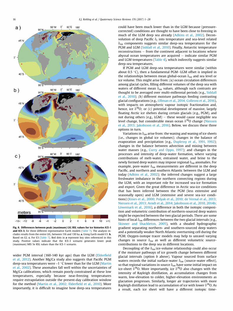
Fig. 8. Differences between peak (maximum) LIG RSL values for ice histories ICE-1and ICE-3, for three different representative Earth models (Table 7). The analysis in-cludes results from the entire LIG, between 116 and 130 ka. a. Using Earth model E1. b.Based on E2. c. For E3 (Table 7). Red dots in a represent key sites referenced in thisstudy. Positive values indicate that the ICE-3 scenario generates lower peak(maximum) MIS 5e RSL values than the ICE-1 scenario.
E.J. Rohling et al. / Quaternary Science Reviews 176 (2017) 1e2816
wider PGM interval (160-140 kyr ago) than the LGM (Elderfieldet al., 2012). Another Mg/Ca study also suggests that Pacific PGMdeep-sea temperatures were ~1 �C lower than for the LGM (Martinet al., 2002). These anomalies fall well within the uncertainties ofMg/Ca calibrations, which remain poorly constrained at these lowtemperatures, especially because near-freezing temperaturesrequire extrapolation outside the present-day calibration windowfor the method (Martin et al., 2002; Elderfield et al., 2010). Moreimportantly, it is difficult to imagine how deep-sea temperatures
could have been much lower than in the LGM because (pressure-corrected) conditions are thought to have been close to freezing inmuch of the LGM deep sea already (Adkins et al., 2002). Decon-volution of deep Pacific dc into temperature and sea-level relateddsw components suggests similar deep-sea temperatures for thePGM and LGM (Siddall et al., 2010). Finally, Antarctic temperaturereconstructions e from the continent adjacent to locations whereabyssal ocean temperatures are acquired e indicate similar PGMand LGM temperatures (Table 4), which indirectly suggests similardeep-sea temperatures.
If PGM and LGM deep-sea temperatures were similar (withinabout 0.5 �C), then a fundamental PGMeLGM offset is implied inthe relationships between mean global-ocean dsw and sea level orice volume. This might arise from: (a) ocean circulation differencesamong glacial cycles, filling different volumes of the deep sea withwaters of different mean dsw values, although such contrasts arethought to be averaged over multi-millennial periods (e.g., Siddallet al., 2010); (b) different moisture pathways feeding contrastingglacial configurations (e.g., Ullman et al., 2014; Colleoni et al., 2016),with impacts on atmospheric vapour isotopic fractionation and,hence, ice d18O; or (c) potential development of massive, largelyfloating Arctic ice shelves during certain glacials (e.g., PGM), andnot during others (e.g., LGM) e these would cause negligible sealevel change, but considerable mean ocean d18O change (Niessenet al., 2013; Jakobsson et al., 2016). Below, we discuss these threeoptions in turn.
Variations in dsw arise from: thewaxing andwaning of ice sheets(i.e., changes in global ice volumes); changes in the balance ofevaporation and precipitation (e.g., Duplessy et al., 1991, 1992);changes in the balance between advection and mixing betweenwater masses (e.g., Curry and Oppo, 1997); and changes in theprocesses and intensity of deep-water formation, where varyingcontributions of melt-water, entrained water, and brine to thenewly formed deep waters may impose regional dsw anomalies. Forexample, pore-water dsw measurements are different in the deepPacific, and northern and southern Atlantic between the LGM andtoday (Adkins et al., 2002); the inferred changes suggest a largefreshwater imbalance in the northern convecting regions duringthe LGM, with an important role for increased sea-ice formationand export. Given the great difference in Arctic sea-ice conditionsthat has been inferred between the PGM (less extensive andseasonally open) and LGM (extensive and severe sea-ice condi-tions) (Knies et al., 2000; Polyak et al., 2010; de Vernal et al., 2013;Niessen et al., 2013; Arndt et al., 2014; Jakobsson et al., 2010, 2014b;L€owemark et al., 2016), a difference in both the isotopic composi-tion and volumetric contribution of northern-sourced deep watersmight be expected between the two glacial periods. There are somehints of local dsw differences between the two glacial intervals (e.g.,Skinner and Shackleton, 2005), with a shoaled hydrographicgradient separating northern- and southern-sourced deep watersand a potentially weaker North Atlantic overturning cell during thePGM. Oxygen-isotope tracer models may help to unravel varyingchanges in source dsw as well as different volumetric source-contributions to the deep sea in different locations.
Decoupling of the dsw:ice-volume relationship could also occurif the moisture pathways of ice growth change between differentglacial intervals (option b above). Vapour sourced from surfacewaters records the initial surface-water dsw (source-water effect),so that regional variations in source dsw have some initial impact onice-sheet d18O. More importantly, ice d18O also changes with theintensity of Rayleigh distillation, as accumulation changes fromwarm, low-elevation to colder, higher-elevation environments asglaciation progresses. Similarly, longer air trajectories with moreRayleigh distillation lead to accumulation of ice with lower d18O. Asa result, each ice sheet will have a different isotopic time-

Table 7Summary of three representative Earth models used in Fig. 8.
EarthModel
Parameterisations Rationale
E1 96 km thick lithosphere VM2-like (Peltier, 2004).5 � 1020 Pa s upper mantle viscosity2.5 � 1021 Pa s lower mantle viscosity
E2 120 km thick lithosphere Closest within suite of earthmodels to a recent preferredearth model for North Americanice history (Lambeck et al., 2017).
5 � 1020 Pa s upper mantle viscosity1.3 � 1022 Pa s lower mantle viscosity
E3 71 km thick lithosphere Closest within suite of earthmodels to recent preferred earthmodel for the last deglaciation(Lambeck et al., 2014).
1.6 � 1020 Pa s upper mantle viscosity5 � 1022 Pa s lower mantle viscosity
E.J. Rohling et al. / Quaternary Science Reviews 176 (2017) 1e28 17
“evolution” (e.g., Mix and Ruddiman, 1984) depending upon theirvolume/height and the latitudinal range over which they expand.As discussed before, the different configurations of the NAIS and EISduring the PGM, relative to the LGM, strongly suggest that theirprocesses of glacial inception and ice-sheet growth were alsodifferent (e.g., Colleoni et al., 2011). Thus, differences in atmo-spheric circulation e and hence moisture supply and degree ofisotopic fractionation e as induced by a lower PGM NAIS may haveaffected the isotopic composition of globally integrated ice volume,leading to potential misrepresentations of both amplitude andtiming of the ice-volume signal (e.g., Mix and Ruddiman, 1984;Clark and Mix, 2002). So far, even the LGM isotopic compositionsof various ice sheets (and their time-evolution) remain poorlyconstrained (e.g., Duplessy et al., 2002; Ferguson and Jasechko,2015), and even less information is available for the PGM. Again,isotope-enabled models may help to characterise the potentialimpact of different moisture-transport pathways and fractionationeffects in the dsw:ice-volume difference between the PGM and LGM.
Contributions from options (a) and (b), outlined above, cannotbe excluded. But option (c), which involves potential developmentof massive, largely floating Arctic ice shelves during the PGM andnot during the LGM, may be particularly important given the largesize and longstanding character of the PGM dc:sea-level discrep-ancy relative to the LGM. Evidence of past floating ice shelves canbe elusive or equivocal because, by their nature, they preserve fewtraces. However, ice-grounding features (e.g., parallel streamlinedsubmarine landforms and ploughmarks) may be preserved in sea-floor sediments, and their occurrence on bathymetric highs, inconjunctionwith regions devoid of glaciogenic seabed disturbance,has been used to suggest evidence of past floating ice (e.g., Polyaket al., 2001; Jakobsson et al., 2008). In the Arctic, erosional fea-tures have been found at depths of ~1 km on the Lomonosov Ridge,Chukchi Borderlands, Yermak Plateau, East Siberian Margin, BaffinBay, and Hovgaard Ridge (Fram Strait) (e.g., Polyak et al., 2001;Kuijpers et al., 2007; Dowdeswell et al., 2010; Gebhardt et al.,2011; Niessen et al., 2013; Arndt et al., 2014), while other por-tions of the Lomonosov andMendeleev Ridges are largely devoid ofglaciogenic features, which may suggest ice-free conditions(Jakobsson et al., 2010). Bathymetric highs in the Arctic may haveacted as pinning points, allowing ice-rise formation that stabilisedand facilitated ice-shelf thickening (Vogt et al., 1994; Grosswaldand Hughes, 1999; Jakobsson et al., 2016).
(Largely) floating Arctic ice shelves during glacial intervals wereproposed in the 1970s and 1980s (Mercer, 1970; Hughes et al., 1977;Broecker, 1975; Grosswald, 1980; Denton and Hughes, 1981;Williams et al., 1981; Chappell and Shackleton, 1986), but thenwere overlooked due to difficulties in obtaining data from the re-gion and a lack of direct evidence for such shelves during the LGM(for an overview, see Jakobsson et al., 2016). Recent geophysical
mapping in the Arctic, however, has led to a re-evaluation of largefloating Arctic ice shelves during the Pleistocene. Various mecha-nisms have been proposed to account for the mapped submarinefeatures, including the drifting of ice-shelf remnants or mega-bergstrapped in multi-year sea ice, or a transient surge or briefgrounding of a floating ice shelf (Polyak et al., 2001, 2009; Engelset al., 2008; Dowdeswell et al., 2010; O'Regan et al., 2010;Gebhardt et al., 2011; Niessen et al., 2013; Dove et al., 2014). Agecontrol for many of the features remains enigmatic, often relying onstratigraphic correlation and biostratigraphy; for example, identi-fication of diagnostic MIS 5e nannofossils gives a likely, or mini-mum, MIS 6 age estimate for features on Morris Jesup Rise,Lomonosov Ridge, Yermak Plateau, Hovgaard Ridge, MendeleevRidge, and Arlis Plateau (Jakobsson, 1999; Polyak et al., 2001;Matthiessen and Knies, 2001; Kristoffersen et al., 2004;Spielhagen et al., 2004; Jakobsson et al., 2008, 2010, 2016; Arndtet al., 2014; L€owemark et al., 2016). Debate continues not onlyabout the age of the submarine features (e.g., Flower, 1997; Niessenet al., 2013), but also about the scale of any ice shelves, from Arctic-wide as proposed by Hughes et al. (1977) and more recently byJakobsson et al. (2016), to (much) more limited extents (Engelset al., 2008; Jakobsson et al., 2010; Niessen et al., 2013; Steinet al., 2017).
The potential presence of an Arctic ice shelf raises questionsabout regional oceanography. Seasonally open waters (leads in theice) are thought to have been continually present in portions of theArctic throughout the last two glacial-interglacial cycles, albeit to alesser degree during glacial periods (Hebbeln and Wefer, 1997;Lloyd et al., 1996; Spielhagen et al., 2004; Knies and Spielhagen,2016). Such open waters may have provided an important mois-ture source for ice growth in Eurasia (Spielhagen et al., 2004). Inorder to reconcile the presence of a large ice shelf with continuedwarm-water advection into the Arctic (Lloyd et al., 1996; Knieset al., 2000; Spielhagen et al., 2004), deepening of the cold halo-cline and advection of Atlantic waters at greater depth than presenthave been proposed (e.g., Jakobsson et al., 2010; Cronin et al., 2012).The Lomonosov Ridge may have acted as a topographic barrier toAtlantic water circulation in the Amerasian Basin, possibly pro-moting ice-shelf growth in this region (Jakobsson et al., 2010).Extensive MIS 6 ice-shelf/shelves covering the central Arctic (e.g.,Hughes et al., 1977; Jakobsson et al., 2016) suggest partial contactwith warmer Atlantic waters in cavities under the ice shelf, anal-ogous to modern Antarctic ice shelves (e.g., Kirschner et al., 2013),with a potential for continued exchange of warmer waters acrossLomonosov Ridge below the grounded ice shelf. Alternatively,Kristoffersen et al. (2004) suggested that advection of warmerAtlantic waters to Lomonosov Ridge during MIS 6 was associatedwith surges or collapses of Saalian ice-sheets, which may havefacilitated northward drift of deep-draft icebergs across Lomonosov

Column Identifier Description
A Identifier Numerical database entry numberB Location Geographic locationC Site Local site nameD Latitude Decimal latitudeE Longitude Decimal longitudeF Lat/Long
estimated?Whether the latitude or longitude of the site isestimated
G Unitdesignation
Stratigraphic unit (as determined by the originalauthors), e.g., Saalian, Warthe etc.
H Feature Type of depositI Reference Publication sourceJ Dating
methodDating method
K Materialdated
The type of material dated
L Reported age(ka)
Calculated age as originally reported
M Ageuncertainty
Age uncertainty as originally reported
N Interpretation Palaeo-environmental interpretation of the deposit (bythe original authors)
E.J. Rohling et al. / Quaternary Science Reviews 176 (2017) 1e2818
Ridge from their discharge areas in the northern Barents-Kararegion.
Overall, the above discussion indicates that evidence forgrounded ice in the Arctic is unequivocal, and some seabed featureshave been attributed to ice-shelf processes (e.g., Polyak et al., 2001;Jakobsson et al., 2010, 2016; Niessen et al., 2013). However, the ageand extent of any Arctic ice-shelves remain elusive, and the exis-tence of Arctic (or even pan-Arctic) ice shelves remains an open andongoing field of research. We investigate what a sea-water-displacing Arctic ice mass/shelf might imply for the dsw:ice-vol-ume relationship for the PGM. First, assuming a modern ArcticOcean area at about 800m depth (5.3� 1012m2) and aworld-oceansurface area of 362 � 1012 m2, our inferred sea-level discrepancybetween the LGM and PGM (~21 mSLE ±14 m at 95% probability)would produce an ice shelf of the correct thickness (~1.4 ± 0.9 km)to account for the observed glacial erosional features in the Arctic.Massive Arctic ice shelves that consist of continental ice with lowd18O values e largely floating, but also as water-displacing groun-ded ice e would alter the relationship between dsw and sea level(and hence, land-based/grounded ice volume) relative to the LGM,even if the relationship between dsw and total (land-based þ floating/water-displacing) global ice volume remainedconstant. It has been estimated that PGM Arctic ice shelves mayhave caused a 0.14 ± 0.03‰ increase in global dsw (and dc), withonly a 0.4 m sea-level impact (Jakobsson et al., 2016). If we use theLGM land-ice-based ratio of 0.009 ± 0.001 m per ‰ (1s) (Adkinset al., 2002; Schrag et al., 2002), then such a dsw anomaly wouldequate to 16 ± 10 m of sea-level change, at 95% probability. Thisagain suggests that our observed Dz ¼ 21 ± 14 m (with indistin-guishable deep-sea d18O) may be largely accounted for by thepresence of massive PGM Arctic ice shelves, and by their absenceduring the LGM. Contribution of both land-based and floating/water-displacing ice volume to PGM dsw (and dc) results in asmaller sea-level drop, while contributions of only land-based iceto LGM dsw (and dc) gives a larger sea-level drop.
5. Conclusions
We provide independent evidence that continental ice volumeson North America (NAIS) and Eurasia (EIS) differed between thePGM and the LGM. During the PGM, the EIS likely reached 33e53mSLE and the NAIS 39e59 mSLE. This compares with reported(Table 1) LGM values of 14e29 and 51e88mSLE for the EIS and NAIS,respectively. Our results provide independent support for theinference that Arctic-wide ice shelves existed during the PGM andnot the LGM, with a previously estimated volume of ~16 mSLE(actual sea-level impact was negligible because the ice was dis-placing seawater). The existence of different ice-sheet configura-tions between Eurasia, North America, and the Arctic implies thatcomplex ice-sheet nucleation processes and growth processes canlead to different glacial modes and that one glacial cycle cannot beused as an analogue for another. Among glacial cycles, we inferdistinctly different relationships between mean global seawaterd18O and global continental ice volume/sea level, and/or betweendeep-sea and Antarctic temperatures. New research using PGM andLGM glaciation ‘modes’may improve understanding of the controlson ice-mass distribution and on Arctic ice-shelf development dur-ing glacial inception. Comparison of the last two glacial cycles witholder glacial cycles is needed to test if there are only two funda-mental modes, or many. Finally, we infer that sea-level studies forthe last interglacial ewhich was warmer and had higher sea levelsthan modern pre-industrial times e may contain considerable biasfrom erroneous assumptions about PGM ice volume and distribu-tion. Depending on the global location of a given site of relative sea-level reconstruction, the adjustment to GIA correction as inferred
here for different ice configurations can be several metres in apositive or negative direction. Results across three representativeEarth models suggest that e if a global assessment were madebased on the sites of LIG sea-level reconstruction considered hereeLIG global mean sea level would be estimated �2 m higher thanconventional estimates (from the same sites) with GIA correctionbased on an LGM-like PGM ice distribution. This requires validationby more complete assessments because it has ramifications forstudies of potential ice-reduction processes that are being used toevaluate sea-level risk in our warming future.
Acknowledgements
This work was supported by Australian Laureate FellowshipFL120100050 (E.J.R.), UK Natural Environment Research Council(NERC) consortium project iGlass (NE/1009906/1 and NE/1008365/1; E.J.R., F.D.H., F.H.W., A.P.R.), Australian Research CouncilDP1094001 (J.M.W.), and Japan Society for the Promotion of ScienceKAKENHI projects JP26247085, and JP15KK0151 (Y.Y.). F.H.W. ac-knowledges constructive discussions withMark Tamisiea regardingthe GIA modelling and results. We thank Tony Purcell (ANU) forproviding LGM and PGM ice-volume estimates reported in Table 1,using the model detailed in Lambeck et al. (2006, 2010, 2017). Ourstudy uses two databases, one on the coral sea-level markers(published in 2016), and the other on glaciomorphological evidence(this study). Both are available via http://www.highstand.org/erohling/ejrhome.htm, where they will be regularly updated. Theglaciomorphological dataset in a fixed form precisely as used in thisstudy is also archived at https://doi.org/10.6084/m9.figshare.5131963.v1.
Appendix I
Appendix 1a. Details and references for the newglaciogeomorphological database
The database contains locations and dates of PGM glaciogenicsediments, or other dated deposits (not necessarily of glacial origin)that directly over- or under-lie glacial deposits relating to the PGM.The database is available directly via the URL listed in the main-textacknowledgements (https://doi.org/10.6084/m9.figshare.5131963.v1). The field descriptors for the database are given in the tablebelow.

E.J. Rohling et al. / Quaternary Science Reviews 176 (2017) 1e28 19
Appendix 1b. Further detail on the GIA analysis
Fig. A1. Range of peak MIS 5e interglacial relative sea levels due to choice of Earth model, for each modelled ice history. a. Output for ICE-1, b. for ICE-2, c. for ICE-3, and d. forICE-4. Red dots in a indicate sea-level reconstruction sites referenced within this study. Each panel illustrates the range of sensitivity of sea-level reconstruction at any given locationto the choice of Earth model, for each ice history. A far greater range of sensitivity exists for choice of Earth model during the LIG for ice histories that contain a larger EIS through thePGM (ICE-3 and ICE-4) than for ICE histories that infer an LGM-like PGM (ICE-1 and ICE-2).
References
Abe-Ouchi, A., Segawa, T., Saito, F., 2007. Climatic conditions for modelling theNorthern Hemisphere ice sheets throughout the ice age cycle. Clim. Past. 3,423e438.
Abe-Ouchi, A., Saito, F., Kawamura, K., Raymo, M.E., Okuno, J.I., Takahashi, K.,Blatter, H., 2013. Insolation-driven 100,000-year glacial cycles and hysteresis ofice-sheet volume. Nature 500, 190e193.
Abe-Ouchi, A., Saito, F., Kageyama, M., Braconnot, P., Harrison, S.P., Lambeck, K.,Otto-Bliesner, B., Peltier, W.R., Tarasov, L., Peterschmitt, J.Y., Takahashi, K., 2015.Ice-sheet configuration in the CMIP5/PMIP3 last glacial maximum experiments.Geosci. Model Dev. 8, 3621e3637.
Adkins, J.F., McIntyre, K., Schrag, D.P., 2002. The salinity, temperature, and d18O ofthe glacial deep ocean. Science 298, 1769e1773.
Ahn, J., Brook, E.J., 2014. Siple Dome ice reveals two modes of millennial CO2 changeduring the last ice age. Nat. Commun. 5, 3732. https://doi.org/10.1038/ncomms4723.
Aitken, M.J., 1998. An Introduction to Optical Dating. The Dating of QuaternarySediments by the Use of Photon-stimulated Luminescence. Oxford UniversityPress, Oxford, 267 pp.
Argus, D.F., Peltier, W.R., Drummond, R., Moore, A.W., 2014. The Antarcticacomponent of postglacial rebound model ICE-6G_C (VM5a) based upon GPSpositioning, exposure age dating of ice thicknesses, and relative sea level his-tories. Geophys. J. Int. 198, 537e563.
Arndt, J.E., Niessen, F., Jokat, W., Dorschel, B., 2014. Deep water paleo-icebergscouring on top of Hovgaard RidgeeArctic Ocean. Geophys. Res. Lett. 41,5068e5074.
Arz, H.W., P€atzold, J., Müller, P.J., Moammar, M.O., 2003. Influence of NorthernHemisphere climate and global sea level rise on the restricted Red Sea marineenvironment during termination I. Paleoceanography 18, 1053,. https://doi.org/10.1029/2002PA000864.
Arz, H.W., Lamy, F., Ganopolski, A., Nowaczyk, N., P€atzold, J., 2007. Dominant
Northern Hemisphere climate control over millennial-scale glacial sea-levelvariability. Quat. Sci. Rev. 26, 312e321.
Astakhov, V., 2001. The stratigraphic framework for the Upper Pleistocene of theglaciated Russian Arctic: changing paradigms. Glob. Planet. Chang. 31, 283e295.
Astakhov, V., 2011. Ice margins of Northern Russia revisited. In: Ehlers, J.,Gibbard, P.L., Hughes, P.D. (Eds.), Quaternary Glaciations e Extent and Chro-nology: a Closer Look. Elsevier, Amsterdam, pp. 323e336. Developments inQuaternary Science 15.
Astakhov, V.I., 2013. Pleistocene glaciations of northern Russiaea modern view.Boreas 42, 1e24.
Astakhov, V., Shkatova, V., Zastrozhnov, A., Chuyko, M., 2016. Glaciomorphologicalmap of the Russian federation. Quat. Int. 420, 4e14.
Balson, S., Jeffery, D.H., 1991. The glacial sequence of the southern North Sea. In:Ehlers, J., Gibbard, P.L., Rose, J. (Eds.), Glacial Deposits in Great Britain andIreland. A. A. Balkema, Rotterdam, pp. 245e254.
Bar-Matthews, M., Ayalon, A., Gilmour, M., Matthews, A., Hawkesworth, C.J., 2003.Seaeland oxygen isotopic relationships from planktonic foraminifera and spe-leothems in the Eastern Mediterranean region and their implication for pale-orainfall during interglacial intervals. Geochim. Cosmochim. Acta 67,3181e3199.
Bar-Or, R., Erlick, C., Gildor, H., 2008. The role of dust in glacialeinterglacial cycles.Quat. Sci. Rev. 27, 201e208.
Bard, E., Hamelin, B., Fairbanks, R.G., Zindler, A., 1990. Calibration of the 14Ctimescale over the past 30,000 years using mass spectrometric U-Th ages fromBarbados corals. Nature 345, 405e410.
Bard, E., Hamelin, B., Arnold, M., Montaggioni, L., Cabioch, G., Faure, G., Rougerie, F.,1996. Deglacial sea-level record from Tahiti corals and the timing of globalmeltwater discharge. Nature 382, 241e244.
Bard, E., Hamelin, B., Delanghe-Sabatier, D., 2010. Deglacial meltwater pulse 1B andYounger Dryas sea levels revisited with boreholes at Tahiti. Science 327,1235e1237.

E.J. Rohling et al. / Quaternary Science Reviews 176 (2017) 1e2820
Barendregt, R.W., Duk-Rodkin, A., 2011. Chronology and extent of Late Cenozoic icesheets in North America: a magnetostratigraphical assessment. In: Ehlers, J.,Gibbard, P.L., Hughes, P.D. (Eds.), Quaternary Glaciations e Extent and Chro-nology: a Closer Look. Elsevier, Amsterdam, pp. 419e426. Developments inQuaternary Science 15.
Bazin, L., Landais, A., Lemieux-Dudon, B., Toy�e Mahamadou Kele, H., Veres, D.,Parrenin, F., Martinerie, P., Ritz, C., Capron, E., Lipenkov, V., Loutre, M.F., 2013. Anoptimized multi-proxy, multi-site Antarctic ice and gas orbital chronology(AICC2012): 120e800 ka. Clim. Past. 9, 1715e1731.
Bintanja, R., van de Wal, R., Oerlemans, J., 2005. Modelled atmospheric tempera-tures and global sea levels over the past million years. Nature 437, 125e128.
Bond, G., Lotti, R., 1995. Iceberg discharges into the North Atlantic on millennialtime scales during the last glaciation. Science 267, 1005e1010.
Braun, D.D., 2011. The glaciation of Pennsylvania, USA. In: Ehlers, J., Gibbard, P.L.,Hughes, P.D. (Eds.), Quaternary Glaciations e Extent and Chronology: a CloserLook. Elsevier, Amsterdam, pp. 521e529. Developments in Quaternary Science15.
Briggs, R.D., Pollard, D., Tarasov, L., 2014. A data-constrained large ensemble analysisof Antarctic evolution since the Eemian. Quat. Sci. Rev. 103, 91e115.
Broecker, W.S., 1975. Floating glacial ice caps in the Arctic Ocean. Science 188,1116e1118.
Buckley, M.W., Marshall, J., 2016. Observations, inferences, and mechanisms of theatlantic meridional overturning circulation: a review. Rev. Geophys. 54, 5e63.
Busschers, F.S., Weerts, H.J.T., Wallinga, J., Cleveringa, P., Kasse, C., Wolf, H.D.,Cohen, K.M., 2005. Sedimentary architecture and optical dating of Middle andLate Pleistocene Rhine-Meuse depositsefluvial response to climate change, sea-level fluctuation and glaciation. Geol. Mijnb. 84, 25e41.
Busschers, F.S., Van Balen, R.T., Cohen, K.M., Kasse, C., Weerts, H.J.T., Wallinga, J.,Bunnik, F.P.M., 2008. Response of the Rhine-Meuse fluvial system to Saalian ice-sheet dynamics. Boreas 37, 377e398.
Calov, R., Ganopolski, A., Kubatzki, C., Claussen, M., 2009. Mechanisms and timescales of glacial inception simulated with an Earth system model of interme-diate complexity. Clim. Past. 5, 245e258.
Carlson, A.E., Winsor, K., 2012. Northern Hemisphere ice-sheet responses to pastclimate warming. Nat. Geosci. 5, 607e613.
Carr, S.J., 2004. the North Sea basin. In: Ehlers, J., Gibbard, P.L. (Eds.), QuaternaryGlaciations Extent and Chronology e Part I: Europe. Elsevier, Amsterdam,pp. 261e270. Developments in Quaternary Sciences 2.
Channell, J.E.T., Hodell, D.A., Romero, O., Hillaire-Marcel, C., de Vernal, A., Stoner, J.S.,Mazaud, A., R€ohl, U., 2012. A 750-kyr detrital-layer stratigraphy for the northatlantic (IODP site U1302-U1303, orphan knoll, labrador sea). Earth Planet. Sci.Lett. 317e318, 218e230.
Chappell, J., Shackleton, N., 1986. Oxygen isotopes and sea level. Nature 324,137e140.
Clague, J.J., Ward, B., 2011. Pleistocene glaciation of british Columbia. In: Ehlers, J.,Gibbard, P.L., Hughes, P.D. (Eds.), Quaternary Glaciations e Extent and Chro-nology: a Closer Look. Elsevier, Amsterdam, pp. 419e426. Developments inQuaternary Science 15.
Clark, P.U., Huybers, P., 2009. Interglacial and future sea level. Nature 462, 856e857.Clark, P.U., Mix, A.C., 2002. Ice sheets and sea level of the last glacial maximum.
Quat. Sci. Rev. 21, 1e7.Clark, P.U., Pollard, D., 1998. Origin of the middle Pleistocene transition by ice sheet
erosion of regolith. Paleoceanography 13, 1e9.Clark, P.U., Tarasov, L., 2014. Closing the sea level budget at the last glacial
maximum. Proc. Natl. Acad. Sci. U. S. A. 111, 15861e15862.Clark, C.D., Evans, D.J., Khatwa, A., Bradwell, T., Jordan, C.J., Marsh, S.H.,
Mitchell, W.A., Bateman, M.D., 2004a. Map and GIS database of glacial land-forms and features related to the last British Ice Sheet. Boreas 33, 359e375.
Clark, C.D., Gibbard, P.L., Rose, J., 2004b. Pleistocene glacial limits in England,Scotland and wales. In: Ehlers, J., Gibbard, P.L. (Eds.), Quaternary Glaciations.Extent and Chronology Part I: Europe. Elsevier, Amsterdam, pp. 47e82. De-velopments in Quaternary Sciences 2.
Clark, P.U., Archer, D., Pollard, D., Blum, J.D., Rial, J.A., Brovkin, V., Mix, A.C.,Pisias, N.G., Roy, M., 2006. The middle Pleistocene transition: characteristics,mechanisms, and implications for long-term changes in atmospheric pCO2.Quat. Sci. Rev. 25, 3150e3184.
Clark, P.U., Dyke, A.S., Shakun, J.D., Carlson, A.E., Clark, J., Wohlfarth, B.,Mitrovica, J.X., Hostetler, S.W., McCabe, A.M., 2009. The last glacial maximum.Science 325, 710e714.
Colleoni, F., Krinner, G., Jakobsson, M., Peyaud, V., Ritz, C., 2009. Influence ofregional parameters on the surface mass balance of the Eurasian ice sheetduring the peak Saalian (140 kya). Glob. Planet. Change 68, 132e148.
Colleoni, F., Liakka, J., Krinner, G., Jakobsson, M., Masina, S., Peyaud, V., 2011. Thesensitivity of the Late Saalian (140 ka) and LGM (21 ka) Eurasian ice sheets tosea surface conditions. Clim. Dyn. 37, 531e553.
Colleoni, F., Masina, S., Cherchi, A., Iovino, D., 2014. Impact of orbital parameters andgreenhouse gas on the climate of MIS 7 and MIS 5 glacial inceptions. J. Clim. 27,8918e8933.
Colleoni, F., Wekerle, C., N€aslund, J.-O., Brandefelt, J., Masina, S., 2016. Constraint onthe penultimate glacial maximum Northern Hemisphere ice topography (z 140kyrs BP). Quat. Sci. Rev. 137, 97e112.
Cook, K.H., Held, I.M., 1988. Stationary waves of the ice age climate. J. Clim. 1,807e819.
Cronin, T.M., Dwyer, G.S., Farmer, J., Bauch, H.A., Spielhagen, R.F., Jakobsson, M.,Nilsson, J., Briggs Jr., W.M., Stepanova, A., 2012. Deep Arctic Ocean warming
during the last glacial cycle. Nat. Geosci. 5, 631e634.Curry, W.B., Oppo, D.W., 1997. Synchronous, high-frequency oscillations in tropical
sea surface temperatures and North Atlantic Deep Water production during thelast glacial cycle. Paleoceanography 12, 1e14.
Curry, B.B., Grimley, D.A., McKay III, E.D., 2011. In: Ehlers, J., Gibbard, P.L.,Hughes, P.D. (Eds.), Quaternary Glaciations e Extent and Chronology: a CloserLook. Elsevier, Amsterdam, pp. 467e487. Developments in Quaternary Science15.
de Boer, B., Van de Wal, R.S.W., Bintanja, R., Lourens, L.J., Tuenter, E., 2010. Cenozoicglobal ice-volume and temperature simulations with 1-D ice-sheet modelsforced by benthic d18O records. Ann. Glaciol. 51, 23e33.
de Boer, B., van de Wal, R.S.W., Lourens, L.J., Bintanja, R., 2012. Transient nature ofthe Earth's climate and the implications for the interpretation of benthic d18Orecords. Palaeogeogr. Palaeoclimatol. Palaeoecol. 335e336, 4e11.
de Boer, B., Lourens, L., van de Wal, R.S., 2014. Persistent 400,000-year variability ofAntarctic ice volume and the carbon cycle is revealed throughout the Plio-Pleistocene. Nat. Commun. 5, 2999,. https://doi.org/10.1038/ncomms3999.
de Vernal, A., Gersonde, R., Goosse, H., Seidenkrantz, M.S., Wolff, E.W., 2013. Sea icein the paleoclimate system: the challenge of reconstructing sea ice fromproxiesean introduction. Quat. Sci. Rev. 79, 1e8.
DeConto, R.M., Pollard, D., 2016. Contribution of Antarctica to past and future sea-level rise. Nature 531, 591e597.
Demidov, 1998 (unpublished e see Svendsen, J.I., Astakhov, V.I., Bolshiyanov, D.Y.,Demidov, I., Dowdeswell, J.A., Gataullin, V., Hjort, C., Hubberten, H.W., Larsen, E.,Mangerud, J., Melles, M., M€oller, P., Saarnisto, M., Siegert, M.J., 1999. Maximumextent of the eurasian ice sheets in the Barents and Kara sea region during theweichselian. Boreas 28, 234e242.
Demidov, I.N., HoumarkeNielsen, M., Kjær, K.H., Funder, S., Larsen, E., Lyså, A.,Lunkka, J.P., Saarnisto, M., 2004. Valdaian glacial maxima in the Arkhangelskdistrict of northwestern Russia. In: Ehlers, J., Gibbard, P.L. (Eds.), QuaternaryGlaciations - Extent and Chronology e Part I: Europe. Elsevier, Amsterdam,pp. 321e336. Developments in Quaternary Sciences 2.
Demidov, I.N., HoumarkeNielsen, M., Kjaer, K.H., Larsen, E., 2006. The last Scandi-navian Ice Sheet in northwestern Russia: ice flow patterns and decay dynamics.Boreas 35, 425e443.
Demuro, M., Froese, D.G., Arnold, L.J., Roberts, R.G., 2012. Single-grain OSL dating ofglaciofluvial quartz constrains Reid glaciation in NW Canada to MIS 6. Quat. Res.77, 305e316.
Dendy, S., Austermann, J., Creveling, J.R., Mitrovica, J.X., 2017. Sensitivity of LastInterglacial sea-level high stands to ice sheet configuration during MarineIsotope Stage 6. Quat. Sci. Rev. 171, 234e244.
Denton, G.H., Hughes, T.J., 1981. Ch. 8. In: Denton, G.H., Hughes, T.J. (Eds.), The LastGreat Ice Sheets. Wiley Interscience, pp. 437e467.
Denton, G.H., Hughes, T.J., 2002. Reconstructing the Antarctic ice sheet at the LastGlacial Maximum. Quat. Sci. Rev. 21, 193e202.
Deschamps, P., Durand, N., Bard, E., Hamelin, B., Camoin, G., Thomas, A.L.,Henderson, G.M., Okuno, J., Yokoyama, Y., 2012. Ice-sheet collapse and sea-levelrise at the Bolling warming 14600 years ago. Nature 483, 559e564.
Dove, D., Polyak, L., Coakley, B., 2014. Widespread, multi-source glacial erosion onthe Chukchi margin, Arctic Ocean. Quat. Sci. Rev. 92, 112e122.
Dowdeswell, J.A., Jakobsson, M., Hogan, K.A., O'Regan, M., Backman, J., Evans, J.,Hell, B., L€owemark, L., Marcussen, C., Noormets, R., Cofaigh, C.�O, 2010. High-resolution geophysical observations of the Yermak Plateau and northern Sval-bard margin: implications for ice-sheet grounding and deep-keeled icebergs.Quat. Sci. Rev. 29, 3518e3531.
Duk-Rodkin, A., Barendregt, R.W., Tarnocai, C., Phillips, F.M., 1996. Late tertiary tolate quaternary record in the Mackenzie Mountains, Northwest Territories,Canada: stratigraphy, paleosols, paleomagnetism, and chlorine-36. Can. J. EarthSci. 33, 875e895.
Duplessy, J.C., Labeyrie, L., Juillet-Leclerc, A., Maitre, F., Duprat, J., Sarnthein, M.,1991. Surface salinity reconstruction of the north-Atlantic ocean during the lastglacial maximum. Oceanol. Acta 14, 311e324.
Duplessy, J.C., Labeyrie, L., Arnold, M., Paterne, M., Duprat, J., van Weering, T.C., 1992.Changes in surface salinity of the North Atlantic Ocean during the last degla-ciation. Nature 358, 485e488.
Duplessy, J.C., Labeyrie, L., Waelbroeck, C., 2002. Constraints on the ocean oxygenisotopic enrichment between the Last Glacial Maximum and the Holocene:paleoceanographic implications. Quat. Sci. Rev. 21, 315e330.
Dutton, A., Lambeck, K., 2012. Ice volume and sea level during the last interglacial.Science 337, 216e219.
Dutton, A., Carlson, A.E., Long, A.J., Milne, G.A., Clark, P.U., DeConto, R., Horton, B.P.,Rahmstorf, S., Raymo, M.E., 2015a. Sea-level rise due to polar ice-sheet massloss during past warm periods. Science 349. https://doi.org/10.1126/science.aaa4019.
Dutton, A., Webster, J.M., Zwartz, D., Lambeck, K., Wohlfarth, B., 2015b. Tropicaltales of polar ice: evidence of last interglacial polar ice sheet retreat recorded byfossil reefs of the granitic Seychelles islands. Quat. Sci. Rev. 107, 182e196.
Dyke, A.S., Andrews, J.T., Clark, P.U., England, J.H., Miller, G.H., Shaw, J., Veillette, J.J.,2002. The Laurentide and Innuitian ice sheets during the last glacial maximum.Quat. Sci. Rev. 21, 9e31.
Ehlers, J., Gibbard, P.L., 2007. The extent and chronology of Cenozoic global glaci-ation. Quat. Int. 164, 6e20.
Ehlers, L., Eissmann, L., Lippstreu, L., Stephan, H.eJ., Wansa, S., 2004. Pleistoceneglaciations of north Germany. In: Ehlers, J., Gibbard, P.L. (Eds.), QuaternaryGlaciations. Extent and Chronology Part I: Europe. Elsevier, Amsterdam,

E.J. Rohling et al. / Quaternary Science Reviews 176 (2017) 1e28 21
pp. 135e146. Developments in Quaternary Science 2.Developments in Quaternary Science 15. In: Ehlers, J., Gibbard, P.L., Hughes, P.D.
(Eds.), 2011a. Quaternary Glaciations e Extent and Chronology, a Closer Look.Elsevier, Amsterdam, 1108 pp.
Ehlers, J., Grube, A., Stephan, H.J., Wansa, S., 2011b. Pleistocene glaciations of NorthGermany e new results. In: Ehlers, J., Gibbard, P.L., Hughes, P.D. (Eds.), Qua-ternary Glaciations e Extent and Chronology: a Closer Look. Elsevier, Amster-dam, pp. 149e162. Developments in Quaternary Science 15.
Elderfield, H., Greaves, M., Barker, S., Hall, I.R., Tripati, A., Ferretti, P., Crowhurst, S.,Booth, L., Daunt, C., 2010. A record of bottom water temperature and seawaterd18O for the Southern Ocean over the past 440 kyr based on Mg/Ca of benthicforaminiferal Uvigerina spp. Quat. Sci. Rev. 29, 160e169.
Elderfield, H., Ferretti, P., Greaves, M., Crowhurst, S., McCave, I.N., Hodell, D.,Piotrowski, A.M., 2012. Evolution of ocean temperature and ice volume throughthe Mid-Pleistocene Climate Transition. Science 337, 704e709.
Engels, J.L., Edwards, M.H., Polyak, L., Johnson, P.D., 2008. Seafloor evidence for iceshelf flow across the AlaskaeBeaufort margin of the Arctic Ocean. Earth Surf.Proc. Landf. 33, 1047e1063.
Fabel, D., Harbor, J., 1999. The use of in-situ produced cosmogenic radionuclides inglaciology and glacial geomorphology. Ann. Glaciol. 28, 103e110.
Fairbanks, R.G., 1989. A 17,000-year glacio-eustatic sea level record: influence ofglacial melting rates on the Younger Dryas event and deep-ocean circulation.Nature 342, 637e642.
Fairbanks, R.G., Mortlock, R.A., Chiu, T.C., Cao, L., Kaplan, A., Guilderson, T.P.,Fairbanks, T.W., Bloom, A.L., Grootes, P.M., Nadeau, M.J., 2005. Radiocarboncalibration curve spanning 0 to 50,000 years BP based on paired230Th/234U/238U and 14C dates on pristine corals. Quat. Sci. Rev. 24, 1781e1796.
Fenton, M., Geiselhart, S., Rohling, E.J., Hemleben, C., 2000. Aplanktonic zones in thered sea. Mar. Micropal 40, 277e294.
Ferguson, G., Jasechko, S., 2015. The isotopic composition of the Laurentide IceSheet and fossil groundwater. Geophys. Res. Lett. 42, 4856e4861.
Flower, B.P., 1997. Overconsolidated section on the Yermak Plateau, Arctic Ocean: icesheet grounding prior to ca. 660 ka? Geology 25, 147e150.
Friedrich, T., Timmermann, A., Tigchelaar, M., Timm, O.E., Ganopolski, A., 2016.Nonlinear climate sensitivity and its implications for future greenhousewarming. Sci. Adv. 2, e1501923,. https://doi.org/10.1126/sciadv.1501923.
Fugitt, F.L., Spahr, P.N., Pavey, R.R., Aden, D.J., Jones, M., Angle, M.P., 2016. SurficalGeology of the Hillsboro 30 X 60-minute Quadrangle in Ohio. Ohio Departmentof Natural Resources, Columbus. Division of Geological Survey Map SG-2-HIL,scale 1:100,000.
Gallimore, R.G., Kutzbach, J.E., 1996. Role of orbitally induced changes in tundra areain the onset of glaciation. Nature 381, 503e505.
Ganopolski, A., Calov, R., 2011. The role of orbital forcing, carbon dioxide andregolith in 100 kyr glacial cycles. Clim. Past. 7, 1415e1425.
Gaunt, G.D., Fletcher, T.P., Wood, C.J., 1992. Geology of the country around kingstonupon hull and brigg. Brit. Geol. Surv. Mem. 172. HMSO, London.
Gebhardt, A.C., Jokat, W., Niessen, F., Matthießen, J., Geissler, W.H., Schenke, H.W.,2011. Ice sheet grounding and iceberg plow marks on the northern and centralYermak Plateau revealed by geophysical data. Quat. Sci. Rev. 30, 1726e1738.
Gemmell, A.M.D., 1988. Thermoluminescence dating of glacially transported sedi-ments: some considerations. Quat. Sci. Rev. 7, 277e285.
Gey, V., Saarnisto, M., Lunkka, J.P., Demidov, I., 2001. Mikulino and Valdai palae-oenvironments in the Vologda area, NW Russia. Glob. Planet. Change 31,347e366.
Gey, V.P., Kozlov, V.V., Malakhovsky, D.B., 2004. On the age and extent of themaximum Late Pleistocene ice advance along the BalticeCaspian watershed. In:Ehlers, J., Gibbard, P.L. (Eds.), Quaternary Glaciations Extent and Chronology ePart I: Europe. Elsevier, Amsterdam, pp. 355e358. Developments in QuaternarySciences 2.
Gibbard, P.L., Clark, C.D., 2011. Pleistocene glaciation limits in great britain. In:Ehlers, J., Gibbard, P.L., Hughes, P.D. (Eds.), Quaternary Glaciations e Extent andChronology: a Closer Look. Elsevier, Amsterdam, pp. 75e94. Developments inQuaternary Science 15.
Gibbard, P.L., Cohen, K.M., 2008. Global chronostratigraphical correlation table forthe last 2.7 million years. Episodes 31, 243e247.
Gibbard, P.L., West, R.G., Andrew, R., Pettit, M., 1992. The margin of a middlePleistocene ice advance at Tottenhill, Norfolk, England. Geol. Mag. 129, 59e76.
Gibbard, P.L., Pasanen, A.H., West, R.G., Lunkka, J.P., Boreham, S., Cohen, K., Rolfe, C.,2009. Late middle Pleistocene glaciation in east Anglia, England. Boreas 38,504e528.
Glen, J.W., 1958. The flow law of ice: a discussion of the assumptions made in glaciertheory, their experimental foundations and consequences. IASH Publ. 47,171e183.
Gosse, J.C., Phillips, F.M., 2001. Terrestrial in situ cosmogenic nuclides: theory andapplication. Quat. Sci. Rev. 20, 1475e1560.
Grant, K.M., Rohling, E.J., Bar-Matthews, M., Ayalon, A., Medina-Elizalde, M.,Ramsey, C.B., Satow, C., Roberts, A.P., 2012. Rapid coupling between ice volumeand polar temperature over the past 150 kyr. Nature 491, 744e747.
Grant, K.M., Rohling, E.J., Ramsey, C.B., Cheng, H., Edwards, R.L., Florindo, F.,Heslop, D., Marra, F., Roberts, A.P., Tamisiea, M.E., Williams, F., 2014. Sea-levelvariability over five glacial cycles. Nat. Commun. 5, 5076.
Grosswald, M.G., 1980. Late Weichselian ice sheets of northern Eurasia. Quat. Res.13, 1e32.
Grosswald, M.G., Hughes, T.J., 1999. The case for an ice shelf in the Pleistocene ArcticOcean 1. Polar Geogr. 23, 23e54.
Guobyte, R., Satkunas, J., 2011. Pleistocene glaciations in Lithuania. In: Ehlers, J.,Gibbard, P.L., Hughes, P.D. (Eds.), Quaternary Glaciations e Extent and Chro-nology: a Closer Look. Elsevier, Amsterdam, pp. 231e246. Developments inQuaternary Science 15.
Gurski, B.N., Levkov, E.A., Karabanov, A.K., Bessarab, D.A., 1990. New data aboutglaciations limits within the Belarus territory. Dokl. Akad. Nauk. Belarusi 34,345e348 (in Russian).
Hansen, J., Sato, M., Kharecha, P., Russell, G., Lea, D.W., Siddall, M., 2007. Climatechange and trace gases. Phil. Trans. R. Soc. Lond. A 365, 1925e1954.
Hansen, J., Sato, M., Kharecha, P., Beerling, D., Berner, R., Masson-Delmotte, V.,Pagani, M., Raymo, M., Royer, D.L., Zachos, J.C., 2008. Target atmospheric CO2:where should humanity aim? Open Atmos. Sci. J. 2, 217e231.
Hansen, J., Sato, M., Russell, G., Kharecha, P., 2013. Climate sensitivity, sea level, andatmospheric carbon dioxide. Phil. Trans. R. Soc. A 371, 20120294. https://doi.org/10.1098/rsta.2012.0294.
Hansen, J., Sato, M., Kharecha, P., von Schuckmann, K., Beerling, D.J., Cao, J.,Marcott, S., Masson-Delmotte, V., Prather, M.J., Rohling, E.J., Shakun, J., Smith, P.,Lacis, A., Russell, G., Ruedy, R., 2017. Young people's burden: requirement ofnegative CO2 emissions. Earth Syst. Dyn. 8, 577e616.
Harris, S.A., 2005. Thermal history of the Arctic Ocean environs adjacent to NorthAmerica during the last 3.5 Ma and a possible mechanism for the cause of thecold events (major glaciations and permafrost events). Prog. Phys. Geogr. 29,218e237.
Hatfield, R.G., Reyes, A.V., Stoner, J.S., Carlson, A.E., Beard, B.L., Winsor, K., Welke, B.,2016. Interglacial responses of the southern Greenland ice sheet over the last430,000 years determined using particle-size specific magnetic and isotopictracers. Earth Planet. Sci. Lett. 454, 225e236.
Hebbeln, D., Wefer, G., 1997. Late quaternary paleoceanography in the Fram Strait.Paleoceanography 12, 65e78.
Hemming, S.R., 2004. Heinrich events: massive late Pleistocene detritus layers ofthe North Atlantic and their global climate imprint. Rev. Geophys 42, RG1005.https://doi.org/10.1029/2003RG000128.
Hennekam, R., 2015. High-frequency climate variability in the late Quaternaryeastern Mediterranean e associations of Nile discharge and basin overturningcirculation dynamics. Utrecht Stud. Earth Sci. 78, 160 pp., ISBN 978-90-6266-390-3.
Hibbert, F.D., Rohling, E.J., Dutton, A., Williams, F.H., Chutcharavan, P.M., Zhao, C.,Tamisiea, M.E., 2016. Corals as indicators of past sea-level change: a globalrepository of U-series dated benchmarks. Quat. Sci. Rev. 145, 1e56.
Hoffman, J.S., Clark, P.U., Parnell, A.C., He, F., 2017. Regional and global sea-surfacetemperatures during the last interglaciation. Science 355, 276e279.
HoumarkeNielsen, M., 2011. Pleistocene glaciations in Denmark: a closer look atchronology, ice dynamics and landforms. In: Ehlers, J., Gibbard, P.L., Hughes, P.D.(Eds.), Quaternary Glaciations e Extent and Chronology: a Closer Look. Elsevier,Amsterdam, pp. 47e58. Developments in Quaternary Science 15.
Hughes, T.J., Denton, G.H., Grosswald, M.G., 1977. Was there a late-Würm Arctic icesheet? Nature 266, 596e602.
Hughes, P.D., Gibbard, P.L., Ehlers, J., 2013. Timing of glaciation during the last glacialcycle: evaluating the concept of a global ‘Last Glacial Maximum’ (LGM). Earth-Sci. Rev. 125, 171e198.
Huybers, P., 2006. Early Pleistocene glacial cycles and the integrated summerinsolation forcing. Science 313, 508e511.
Huybrechts, P., 2002. Sea-level changes at the LGM from ice-dynamic re-constructions of the Greenland and Antarctic ice sheets during the glacial cy-cles. Quat. Sci. Rev. 21, 203e231.
Imbrie, J., Hays, J.D., Martinson, D.G., McIntyre, A., Mix, A.C., Morley, J.J., Pisias, N.G.,Prell, W.L., Shackleton, N.J., 1984. The orbital theory of Pleistocene climate:support from a revised chronology of the marine d18O record. In: Berger, A.(Ed.), Milankovitch and Climate, Part I. Springer, New York, pp. 269e305.
Imbrie, J., Berger, A., Boyle, E.A., Clemens, S.C., Duffy, A., Howard, W.R., Kukla, G.,Kutzbach, J., Martinson, D.G., McIntyre, A., Mix, A.C., Molfino, B., Morley, J.J.,Peterson, L.C., Pisias, N.G., Prell, W.L., Raymo, M.E., Shackleton, N.J.,Toggweiler, J.R., 1993. On the structure and origin of major glaciation cycles. 2,the 100,000-year cycle. Paleoceanography 8, 699e735.
Israelson, C., Wohlfarth, B., 1999. Timing of the last-interglacial high sea level on theSeychelles Islands, Indian Ocean. Quat. Res. 51, 306e316.
Ivins, E.R., James, T.S., 2005. Antarctic glacial isostatic adjustment: a new assess-ment. Antarct. Sci. 17, 541e553.
Jackson, L., Ward, B., Duk-Rodkin, A., Hughes, O., 1991. The last Cordilleran ice sheetin southern Yukon Territory. G�eogr. Phys. Quat. 45, 341e354.
Jackson, L.E., Andriashek, L.D., Phillips, F.M., 2011. Limits of successive Middle andLate Pleistocene continental ice sheets, interior plains of southern and centralAlberta and adjacent areas. In: Ehlers, J., Gibbard, P.L., Hughes, P.D. (Eds.),Quaternary Glaciations e Extent and Chronology: a Closer Look. Elsevier,Amsterdam, pp. 575e590. Developments in Quaternary Science 15.
Jakobsson, M., 1999. First high-resolution CHIRP sonar profiles from the centralArctic Ocean reveal erosion of Lomonosov Ridge sediments. Mar. Geol. 158,111e123.
Jakobsson, M., Polyak, L., Edwards, M., Kleman, J., Coakley, B., 2008. Glacial geo-morphology of the central Arctic Ocean: the Chukchi borderland and theLomonosov Ridge. Earth Surf. Proc. Landf. 33, 526e545.
Jakobsson, M., Nilsson, J., O'Regan, M., Backman, J., L€owemark, L., Dowdeswell, J.A.,Mayer, L., Polyak, L., Colleoni, F., Anderson, L.G., Bj€ork, G., 2010. An Arctic Oceanice shelf during MIS 6 constrained by new geophysical and geological data.Quat. Sci. Rev. 29, 3505e3517.
E.J. Rohling et al. / Quaternary Science Reviews 176 (2017) 1e2822
Jakobsson, M., Andreassen, K., Bjarnad�ottir, L.R., Dove, D., Dowdeswell, J.A.,England, J.H., Funder, S., Hogan, K., Ing�olfsson, �O., Jennings, A., Larsen, N.K.,2014a. Arctic Ocean glacial history. Quat. Sci. Rev. 92, 40e67.
Jakobsson, M., Ing�olfsson, �O., Long, A.J., Spielhagen, R.F., 2014b. The dynamic Arctic.Quat. Sci. Rev. 92, 1e8.
Jakobsson, M., Nilsson, J., Anderson, L., Backman, J., Bj€ork, G., Cronin, T.M.,Kirchner, N., Koshurnikov, A., Mayer, L., Noormets, R., O'Regan, M., 2016. Evi-dence for an ice shelf covering the central Arctic Ocean during the penultimateglaciation. Nat. Commun. 7, 10365.
Kageyama, M., Valdes, P.J., 2000. Impact of the North American ice-sheet orographyon the Last Glacial Maximum eddies and snowfall. Geophys. Res. Lett. 27,1515e1518.
Kageyama, M., Valdes, P.J., Ramstein, G., Hewitt, C., Wyputta, U., 1999. NorthernHemisphere storm tracks in present day and last glacial maximum climatesimulations: a comparison of the European PMIP models. J. Clim. 12, 742e760.
Karabanov, A.K., Matveyev, A.V., 2011. The Pleistocene glaciations in Belarus. In:Ehlers, J., Gibbard, P.L., Hughes, P.D. (Eds.), Quaternary Glaciations e Extent andChronology: a Closer Look. Elsevier, Amsterdam, pp. 29e35. Developments inQuaternary Science 15.
Kendall, R.A., Mitrovica, J.X., Milne, G.A., 2005. On post-glacial sea level e II. Nu-merical formulation and comparative results on spherically symmetric models.Geophys. J. Int. 161, 679e706.
Kirschner, N., Furrer, R., Jakobsson, M., Zwally, H.J., Robbins, J.W., 2013. Statisticalmodeling of a former Arctic Ocean ice shelf complex using Antarctic analogies.J. Geophys. Res. 118, 1105e1117.
Knies, J., Spielhagen, R.F., 2016. A pan-Arctic ice shelf during late Marine IsotopeStage (MIS) 6: fact or fiction?. In: Abstracts, Past Gateways 4th InternationalConference, pp. 45e46. Trondheim, Norway, 23e27 May 2016.
Knies, J., Nowaczyk, N., Müller, C., Vogt, C., Stein, R., 2000. A multiproxy approach toreconstruct the environmental changes along the Eurasian continental marginover the last 150 000 years. Mar. Geol. 163, 317e344.
Knight, J., Coxon, P., McCabe, A.M., McCarron, S.G., 2004. Pleistocene glaciations inIreland. In: Ehlers, J., Gibbard, P.L. (Eds.), Quaternary Glaciations Extent andChronology e Part I: Europe. Elsevier, Amsterdam, pp. 183e191. Developmentsin Quaternary Sciences, 2.
K€ohler, P., Bintanja, R., Fischer, H., Joos, F., Knutti, R., Lohmann, G., Masson-Delmotte, V., 2010. What caused Earth's temperature variations during the last800,000 years? Data-based evidence on radiative forcing and constraints onclimate sensitivity. Quat. Sci. Rev. 29, 129e145.
K€ohler, P., de Boer, B., von der Heydt, A.S., Stap, L.B., van de Wal, R., 2015. On thestate dependency of the equilibrium climate sensitivity during the last 5 millionyears. Clim. Past. 11, 1801e1823.
K€ohler, P., Bintanja, R., 2008. The carbon cycle during the mid Pleistocene transi-tion: the southern ocean decoupling hypothesis. Clim. Past. 4, 311e332.
Krinner, G., Mangerud, J., Jakobsson, M., Crucifix, M., 2004. Enhanced ice sheetgrowth in Eurasia owing to adjacent ice-dammed lakes. Nature 427, 429e432.
Krinner, G., Boucher, O., Balkanski, Y., 2006. Ice-free glacial northern Asia due todust deposition on snow. Clim. Dyn. 27, 613e625.
Kristoffersen, Y., Coakley, B., Jokat, W., Edwards, M., Brekke, H., Gjengedal, J., 2004.Seabed erosion on the Lomonosov Ridge, central Arctic Ocean: a tale of deepdraft icebergs in the Eurasia Basin and the influence of Atlantic water inflow oniceberg motion? Paleoceanography 19. https://doi.org/10.1029/2003PA000985.
Kuijpers, A., Dalhoff, F., Brandt, M.P., Hümbs, P., Schott, T., Zotova, A., 2007. Gianticeberg plow marks at more than 1km water depth offshore West Greenland.Mar. Geol. 246, 60e64.
Laban, C., van der Meer, J.J.M., 2004. Pleistocene glaciation in The Netherlands. In:Ehlers, J., Gibbard, P.L. (Eds.), Quaternary Glaciations Extent and Chronology ePart I: Europe. Elsevier, pp. 251e260. Developments in Quaternary Sciences, 2.
Laban, C., van der Meer, J.J., 2011. Pleistocene glaciation in The Netherlands. In:Ehlers, J., Gibbard, P.L., Hughes, P.D. (Eds.), Quaternary Glaciations e Extent andChronology: a Closer Look. Elsevier, pp. 247e260. Developments in QuaternaryScience 15.
Lambeck, K., Chappell, J., 2001. Sea level change through the last glacial cycle.Science 292, 679e686.
Lambeck, K., Purcell, A., Funder, S., Kjær, K., Larsen, E., Moller, P.E.R., 2006. Con-straints on the Late Saalian to early Middle Weichselian ice sheet of Eurasiafrom field data and rebound modelling. Boreas 35, 539e575.
Lambeck, K., Purcell, A., Zhao, J., Svensson, N.O., 2010. The scandinavian ice sheet:from MIS 4 to the end of the last glacial maximum. Boreas 39, 410e435.
Lambeck, K., Rouby, H., Purcell, A., Sun, Y., Sambridge, M., 2014. Sea level and globalice volumes from the Last Glacial Maximum to the Holocene. Proc. Natl. Acad.Sci. U.S.A. 111, 15296e15303.
Lambeck, K., Purcell, A., Zhao, S., 2017. The North American Late Wisconsin ice sheetand mantle viscosity from glacial rebound analyses. Quat. Sci. Rev. 158,172e210.
Landais, A., Dreyfus, G., Capron, E., Jouzel, J., Masson-Delmotte, V., Roche, D.M.,Pri�e, F., Caillon, N., Chappellaz, J., Leuenberger, M., Lourantou, A., 2013. Two-phase change in CO2, Antarctic temperature and global climate during Termi-nation II. Nat. Geosci. 6, 1062e1065.
Larrasoa~na, J.C., Roberts, A.P., Rohling, E.J., Winklhofer, M., Wehausen, R., 2003.Three million years of monsoon variability over the northern Sahara. Clim. Dyn.21, 689e698.
Laskar, J., Robutel, P., Joutel, F., Gastineau, M., Correia, A.C.M., Levrard, B., 2004.A long-term numerical solution for the insolation quantities of the Earth.Astron. Astrophys. 428, 261e285.
Le Roy, I., 1994. Evolution des volcans en syst�eme de point chaud: île de Tahiti,Archipel de la Soci�et�e (Polyn�esie Française). PhD thesis. University of Paris, 271pp.
Lecavalier, B.S., Milne, G.A., Simpson, M.J., Wake, L., Huybrechts, P., Tarasov, L.,Kjeldsen, K.K., Funder, S., Long, A.J., Woodroffe, S., Dyke, A.S., 2014. A model ofGreenland ice sheet deglaciation constrained by observations of relative sealevel and ice extent. Quat. Sci. Rev. 102, 54e84.
Liakka, J., Nilsson, J., L€ofverstr€om, M., 2012. Interactions between stationary wavesand ice sheets: linear versus nonlinear atmospheric response. Clim. Dyn. 38,1249e1262.
Liakka, J., L€overstr€om, M., Colleoni, F., 2016. The impact of the North Americanglacial topography on the evolution of the Eurasian ice sheet over the lastglacial cycle. Clim. Past. 12, 1225e1241.
Licciardi, J.M., Clark, P.U., Jenson, J.W., Macayeal, D.R., 1998. Deglaciation of a soft-bedded Laurentide ice sheet. Quat. Sci. Rev. 17, 427e448.
Lippstreu, L., 2002 (unpublished e see Lippstreu, L., Brose, F., Marcinek, J., 1995.Brandenburg. Das Quart€ar Deutschlands, 116e147.).
Lisiecki, L.E., Raymo, M.E., 2005. A Pliocene-Pleistocene stack of 57 globallydistributed benthic d18O records. Paleoceanography 20, PA1003,. https://doi.org/10.1029/2004PA001071.
Litt, T., Behre, K.-E., Meyer, K.-D., Stephan, H.-J., Wansa, S., 2007. StratigraphisheBegriffe für das Quart€ar des Norddeutschland Vereisungsgebietes. Quat. Sci. J.56, 7e65.
Liverman, D.G., Catto, N.R., Rutter, N.W., 1989. Laurentide glaciation in west-centralAlberta: a single (Late Wisconsinan) event. Canad. J. Earth Sci. 26, 266e274.
Lloyd, J.M., Kroon, D., Boulton, G.S., Laban, C., Fallick, A., 1996. Ice rafting historyfrom the Spitsbergen ice cap over the last 200 kyr. Mar. Geol. 131, 103e121.
L€ofverstr€om, M., Caballero, R., Nilsson, J., Kleman, J., 2014. Evolution of the large-scale atmospheric circulation in response to changing ice sheets over the lastglacial cycle. Clim. Past. 10, 1453e1471.
Loulergue, L., Schilt, A., Spahni, R., Masson-Delmotte, V., Blunier, T., Lemieux, B.,Barnola, J.M., Raynaud, D., Stocker, T.F., Chappellaz, J., 2008. Orbital andmillennial-scale features of atmospheric CH4 over the past 800,000 years. Na-ture 453, 383e386.
Lourantou, A., Lavric, J.V., Koehler, P., Barnola, J.-M., Paillard, D., Michel, E.,Raynaud, D., Chappellaz, J., 2010. Constraint of the CO2 rise by new atmosphericcarbon isotopic measurements during the last deglaciation. Glob. Biogeochem.Cycles 24. https://doi.org/10.1029/2009GB003545.
L€owemark, L., Chao, W.S., Gyllencreutz, R., Hanebuth, T.J.J., Chiu, P.Y., Yang, T.N.,Su, C.C., Chuang, C.K., Dominguez, D.C., Jakobsson, M., 2016. Variations in glacialand interglacial marine conditions over the last two glacial cycles off northernGreenland. Quat. Sci. Rev. 147, 164e177.
Mangerud, J., Astakhov, V., Svendsen, J.I., 2002. The extent of the barentsekara icesheet during the last glacial maximum. Quat. Sci. Rev. 21, 111e119.
Mangerud, J., Jakobsson, M., Alexanderson, H., Astakhov, V., Clarke, G.K.,Henriksen, M., Hjort, C., Krinner, G., Lunkka, J.P., M€oller, P., Murray, A., 2004. Ice-dammed lakes and rerouting of the drainage of northern Eurasia during the LastGlaciation. Quat. Sci. Rev. 23, 1313e1332.
Marino, G., Rohling, E.J., Rodríguez-Sanz, L., Grant, K.M., Heslop, D., Roberts, A.P.,Stanford, J.D., Yu, J., 2015. Bipolar seesaw control on last interglacial sea level.Nature 522, 197e201.
Marks, L., 2011. Quaternary glaciations in Poland. Dev. Quat. Sci. 15, 299e303.Marks, L., 2012. Timing of the late vistulian (weichselian) glacial phases in Poland.
Quat. Sci. Rev. 44, 81e88.Marshall, S.J., Clark, P.U., 2002. Basal temperature evolution of North American ice
sheets and implications for the 100-kyr cycle. Geophys. Res. Lett. 29, 671e674.Marshall, S.J., James, T.S., Clarke, G.K., 2002. North American ice sheet re-
constructions at the last glacial maximum. Quat. Sci. Rev. 21, 175e192.Martin, P.A., Lea, D.W., Rosenthal, Y., Shackleton, N.J., Sarnthein, M., Papenfuss, T.,
2002. Quaternary deep sea temperature histories derived from benthic fora-miniferal Mg/Ca. Earth Planet. Sci. Lett. 198, 193e209.
Martínez-Botí, M.A., Foster, G.L., Chalk, T.B., Rohling, E.J., Sexton, P.F., Lunt, D.J.,Pancost, R.D., Badger, M.P.S., Schmidt, D.N., 2015. Plio-Pleistocene climatesensitivity evaluated using high-resolution CO2 records. Nature 518, 49e54.
Martinson, D.G., Pisias, N.G., Hays, J.D., Imbrie, J., Moore, T.C., Shackleton, N.J., 1987.Age dating and the orbital theory of the ice ages: development of a high-resolution 0 to 300,000-year chronostratigraphy. Quat. Res. 27, 1e29.
Matoshko, A.V., 2011. Chapter 31. Limits of the Pleistocene glaciation in the Ukraine:a closer look. In: Ehlers, J., Gibbard, P.L., Hughes, P.D. (Eds.), Quaternary Glaci-ations e Extent and Chronology: a Closer Look. Elsevier, Amsterdam,pp. 405e416. Developments in Quaternary Science 15.
Matoshko, A.V., Chugunny, Yu G., 1993. The Dnieper Glaciation of Ukraine(Geological Aspect). Naukova Dumka, Kiev, p. 192 (In Russian).
Matoshko, A.V., Chugunny, Yu G., 1995. Geological activity and dynamic evolution ofthe Dnieper glaciation. In: Ehlers, J., Kozarski, S., Gibbard, P.L. (Eds.), GlacialDeposits in NortheEast Europe. A.A. Balkema, Rotterdam, Brookfield,pp. 225e230.
Matthiessen, J., Knies, J., 2001. Dinoflagellate cyst evidence for warm interglacialconditions at the northern Barents Sea margin during marine oxygen isotopestage 5. J. Quat. Sci. 16, 727e737.
McKay III, E.D., Berg, R.C., 2008. Optical ages spanning two glacial-interglacial cyclesfrom deposits of the ancient Mississippi river, north-central Illinois. Geol. Soc.Am. Abstr. Progr 40, 78.
McKay III, E.D., Berg, R.C., Hansel, A.K., Kemmis, T.J., Stumpf, A.J., 2008. Quaternarydeposits and history of the ancient Mississippi river valley, north-central

E.J. Rohling et al. / Quaternary Science Reviews 176 (2017) 1e28 23
Illinois. Ill. State Geol. Surv. Guideb. 35, 106 pp.McKay, N.P., Overpeck, J.T., Otto-Bliesner, B.L., 2011. The role of ocean thermal
expansion in Last Interglacial sea level rise. Geophys. Res. Lett. 38, L14605.https://doi.org/10.1029/2011GL048280.
Mercer, J.H., 1970. A former ice sheet in the Arctic Ocean? Palaeogeogr. Palae-oclimatol. Palaeoecol. 8, 19e27.
Mitrovica, J.X., Wahr, J., Matsuyama, I., Paulson, A., 2005. The rotational stability ofan ice-age earth. Geophys. J. Int. 161, 491e506.
Mix, A.C., Ruddiman, W.F., 1984. Oxygen-isotope analyses and Pleistocene ice vol-umes. Quat. Res. 21, 1e20.
Mix, A.C., Bard, E., Schneider, R., 2001. Environmental processes of the ice age: land,oceans, glaciers (EPILOG). Quat. Sci. Rev. 20, 627e657.
Mohr, K., 1993. Terti€ar und Quart€ar. In: Mohr, K. (Ed.), Geologie und Miner-allagerst€atten des Harzes. Schweizerbart Science Publications, Stuttgart, p. 384.
M€oller, P., Alexanderson, H., Funder, S., Hjort, C., 2015. The Taimyr Peninsula and theSevernaya Zemlya archipelago, Arctic Russia: a synthesis of glacial history andpalaeo-environmental change during the Last Glacial cycle (MIS 5ee2). Quat.Sci. Rev. 107, 149e181.
Monnin, E., Indermühle, A., D€allenbach, A., Flückiger, J., Stauffer, B., Stocker, T.F.,Raynaud, D., Barnola, J.M., 2001. Atmospheric CO2 concentrations over the lastglacial termination. Science 291, 112e114.
Monnin, E., Steig, E.J., Siegenthaler, U., Kawamura, K., Schwander, J., Stauffer, B.,Stocker, T.F., Morse, D.L., Barnola, J.M., Bellier, B., Raynaud, D., Fischer, H., 2004.Evidence for substantial accumulation rate variability in Antarctica during theHolocene, through synchronization of CO2 in the Taylor Dome, Dome C andDML ice cores. Earth Planet. Sci. Lett. 224, 45e54.
Montaggioni, L.F., 2005. History of Indo-Pacific coral reef systems since the lastglaciation: development patterns and controlling factors. Earth Sci. Rev. 71,1e75.
Naafs, B.D.A., Hefter, J., Acton, G., Haug, G.H., Martínez-Garcia, A., Pancost, R.,Stein, R., 2012. Strengthening of north american dust sources during the latePliocene (2.7 ma). Earth Planet. Sci. Lett. 317, 8e19.
Niessen, F., Hong, J.K., Hegewald, A., Matthiessen, J., Stein, R., Kim, H., Kim, S.,Jensen, L., Jokat, W., Nam, S.I., Kang, S.H., 2013. Repeated Pleistocene glaciationof the east siberian continental margin. Nat. Geosci. 6, 842e846.
Nørgaard-Pedersen, N., Mikkelsen, N., Lassen, S.J., Kristoffersen, Y., Sheldon, E.,2007. Reduced sea ice concentrations in the Arctic Ocean during the lastinterglacial period revealed by sediment cores off northern Greenland. Paleo-ceanography 22, PA1218,. https://doi.org/10.1029/2006PA001283.
O'Regan, M., Jakobsson, M., Kirchner, N., 2010. Glacial geological implications ofoverconsolidated sediments on the Lomonosov Ridge and Yermak plateau.Quat. Sci. Rev. 29, 3532e3544.
Obrochta, S.P., Crowley, T.J., Channell, J.E.T., Hodell, D.A., Baker, P.A., Seki, A.,Yokoyama, Y., 2014. Climate variability and ice-sheet dynamics during the lastthree glaciations. Earth Planet. Sci. Lett. 406, 198e212.
Oglesby, R.J., 1990. Sensitivity of glaciation to initial snow cover, CO2, snow albedo,and oceanic roughness in the NCAR CCM. Clim. Dyn. 4, 219e235.
Osborne, A.H., Vance, D., Rohling, E.J., Barton, N., Rogerson, M., Fello, N., 2008.A humid corridor across the Sahara for the migration “Out of Africa” of earlymodern humans 120,000 years ago. Proc. Natl. Acad. Sci. U. S. A. 105,16444e16447.
Palienko, V.P., 1982. Features of glacial relief of the Dnieper glacier marginal zonewithin Volyn' Polessie area. In: Bondarchuk, V.G. (Ed.), Materialy Po IzucheniyuChetvertichnogo Perioda Na Teritorii Ukrainy. Naukova dumka, Kiev,pp. 203e211.
Parrenin, F., Masson-Delmotte, V., K€ohler, P., Raynaud, D., Paillard, D., Schwander, J.,Barbante, C., Landais, A., Wegner, A., Jouzel, J., 2013. Synchronous change ofatmospheric CO2 and Antarctic temperature during the last deglacial warming.Science 339, 1060e1063.
Patton, H., Hubbard, A., Andreassen, K., Winsborrow, M., Stroeven, A.P., 2016. Thebuild-up, configuration, and dynamical sensitivity of the Eurasian ice-sheetcomplex to Late Weichselian climatic and oceanic forcing. Quat. Sci. Rev. 153,97e121.
Pattyn, F., 2010. Antarctic subglacial conditions inferred from a hybrid ice sheet/icestream model. Earth Planet. Sci. Lett. 295, 451e461.
Pavey, R.R., Goldthwait, R.P., Brockman, C.S., Hull, D.N., Swinford, E.M., VanHorn, R.G., 1999. Quaternary Geology of Ohio. Ohio Division of GeologicalSurvey. Map No. 2.
Payne, A.J., 1995. Limit cycles in the basal thermal regime of ice sheets. J. Geophys.Res. 100, 4249e4263.
Peltier, W.R., 1994. Ice age paleotopography. Science 265, 195e201.Peltier, W.R., 1996. Mantle viscosity and ice-age ice sheet topography. Science 273,
1359e1364.Peltier, W.R., 2004. Global glacial isostasy and the surface of the ice-age Earth: the
ICE-5G (VM2) model and GRACE. Ann. Rev. Earth Planet. Sci. 32, 111e149.Peltier, W.R., Argus, D.F., Drummond, R., 2015. Space geodesy constrains ice-age
terminal deglaciation: the global ICE-6G_C (VM5a) model. J. Geophys. Res.120, 450e487.
Peyaud, V., 2006. Role de la dynamique des calottes glaciaires dans les grandschangements climatiques des p�eriodes glaciaires-interglaciaires. PhD thesis.Universit�e Joseph-Fourier-Grenoble, 247 pp.
Polyak, L., Edwards, M.H., Coakley, B.J., Jakobsson, M., 2001. Ice shelves in thePleistocene Arctic Ocean inferred from glaciogenic deep-sea bedforms. Nature410, 453e457.
Polyak, L., Curry, W.B., Darby, D.A., Bischof, J., Cronin, T.M., 2004. Contrasting glacial/
interglacial regimes in the western Arctic Ocean as exemplified by a sedi-mentary record from the Mendeleev Ridge. Palaeogeogr. Palaeoclimatol.Palaeoecol. 203, 73e93.
Polyak, L., Bischof, J., Ortiz, J.D., Darby, D.A., Channell, J.E.T., Xuan, C., Kaufman, D.S.,Løvlie, R., Schneider, D.A., Eberl, D.D., Adler, R.E., 2009. Late Quaternary stra-tigraphy and sedimentation patterns in the western Arctic Ocean. Glob. Planet.Chang. 68, 5e17.
Polyak, L., Alley, R.B., Andrews, J.T., Brigham-Grette, J., Cronin, T.M., Darby, D.A.,Dyke, A.S., Fitzpatrick, J.J., Funder, S., Holland, M., Jennings, A.E., 2010. History ofsea ice in the Arctic. Quat. Sci. Rev. 29, 1757e1778.
Potter, E.K., Lambeck, K., 2003. Reconciliation of sea-level observations in theWestern North Atlantic during the last glacial cycle. Earth Planet. Sci. Lett. 217,171e181.
Putkonen, J., Swanson, T., 2003. Accuracy of cosmogenic ages for moraines. Quat.Res. 59, 255e261.
Rabineau, M., Bern�e, S., Olivet, J.L., Aslanian, D., Guillocheau, F., Joseph, P., 2006.Paleo sea levels reconsidered from direct observation of paleoshoreline positionduring Glacial Maxima (for the last 500,000 yr). Earth Planet. Sci. Lett. 252,119e137.
Raymo, M.E., Lisiecki, L.E., Nisancioglu, K.H., 2006. Plio-Pleistocene ice volume,Antarctic climate, and the global d18O record. Science 313, 492e495.
Reimer, P.J., Bard, E., Bayliss, A., Beck, J.W., Blackwell, P.G., Ramsey, C.B., Buck, C.E.,Cheng, H., Edwards, R.L., Friedrich, M., Grootes, P.M., 2013. INTCAL13 and MA-RINE13 radiocarbon age calibration curves 0-50,000 years cal BP. Radiocarbon55, 1869e1887.
Ringler, T.D., Cook, K.H., 1997. Factors controlling nonlinearity in mechanicallyforced stationary waves over orography. J. Atmos. Sci. 54, 2612e2629.
Roe, G.H., Lindzen, R.S., 2001. The mutual interaction between continental-scale icesheets and atmospheric stationary waves. J. Clim. 14, 1450e1465.
Rohling, E.J., Fenton, M., Jorissen, F.J., Bertrand, P., Ganssen, G., Caulet, J.P., 1998.Magnitudes of sea-level lowstands of the past 500,000 years. Nature 394,162e165.
Rohling, E.J., Cane, T.R., Cooke, S., Sprovieri, M., Bouloubassi, I., Emeis, K.C.,Schiebel, R., Kroon, D., Jorissen, F.J., Lorre, A., Kemp, A.E.S., 2002. Africanmonsoon variability during the previous interglacial maximum. Earth Planet.Sci. Lett. 202, 61e75.
Rohling, E.J., Sprovieri, M., Cane, T., Casford, J.S., Cooke, S., Bouloubassi, I.,Emeis, K.C., Schiebel, R., Rogerson, M., Hayes, A., Jorissen, F.J., 2004. Recon-structing past planktic foraminiferal habitats using stable isotope data: a casehistory for Mediterranean sapropel S5. Mar. Micropal 50, 89e123.
Rohling, E.J., Grant, K., Hemleben, C.H., Siddall, M., Hoogakker, B.A.A., Bolshaw, M.,Kucera, M., 2008. High rates of sea-level rise during the last interglacial period.Nat. Geosci. 1, 38e42.
Rohling, E.J., Grant, K., Bolshaw, M., Roberts, A.P., Siddall, M., Hemleben, C.,Kucera, M., 2009. Antarctic temperature and global sea level closely coupledover the past five glacial cycles. Nat. Geosci. 2, 500e504.
PALAEOSENS Project Members, Rohling, E.J., Sluijs, A., Dijkstra, H.A., K€ohler, P., vande Wal, R.S.W., von der Heydt, A.S., Beerling, D., Berger, A., Bijl, P.K., Crucifix, M.,deConto, R., Drijfhout, S.S., Fedorov, A., Foster, G., Ganopolski, A., Hansen, J.,H€onisch, B., Hooghiemstra, H., Huber, M., Huybers, P., Knutti, R., Lea, D.W.,Lourens, L.J., Lunt, D., Masson-Demotte, V., Medina-Elizalde, M., Otto-Bliesner, B., Pagani, M., P€alike, H., Renssen, H., Royer, D.L., Siddall, M., Valdes, P.,Zachos, J.C., Zeebe, R.E., 2012. Making sense of palaeoclimate sensitivity. Nature491, 683e691.
Rohling, E.J., Medina-Elizalde, M., Shepherd, J.G., Siddall, M., Stanford, J.D., 2012. Seasurface and high-latitude temperature sensitivity to radiative forcing of climateover several glacial cycles. J. Clim. 25, 1635e1656.
Rohling, E.J., Foster, G.L., Grant, K.M., Marino, G., Roberts, A.P., Tamisiea, M.E.,Williams, F., 2014. Sea-level and deep-sea-temperature variability over the past5.3 million years. Nature 508, 477e482.
Rohling, E.J., Marino, G., Grant, K.M., 2015. Mediterranean climate and oceanog-raphy, and the periodic development of anoxic events (sapropels). Earth-Sci.Rev. 143, 62e97.
Rose, J., 2009. Early and middle Pleistocene landscapes of eastern England. Proc.Geol. Assoc. 120, 3e33.
Rose, J., Candy, I., Moorlock, B.S.P., Wilkins, H., Lee, J.A., Hamblin, R.J.O., Lee, J.R.,Riding, J.B., Morigi, A.N., 2002. Early and early Middle Pleistocene river, coastaland neotectonic processes, southeast Norfolk, England. Proc. Geol. Assoc. 113,47e67.
Rovey, C.W., Balco, G., 2011. Summary of early and middle Pleistocene glaciations innorthern Missouri, USA. In: Ehlers, J., Gibbard, P.L., Hughes, P.D. (Eds.), Qua-ternary Glaciations e Extent and Chronology: a Closer Look. Elsevier,pp. 553e562. Developments in Quaternary Science 15.
Ruddiman, W.E., 1977. Late Quaternary deposition of ice-rafted sand in the sub-polar North Atlantic (40-60� N). Geol. Soc. Am. Bull. 88, 1813e1827.
Ruzicka, M., 2004. The Pleistocene glaciation of Czechia. In: Ehlers, J., Gibbard, P.L.(Eds.), Quaternary Glaciations Extent and Chronology e Part I: Europe. Elsevier,Amsterdam, pp. 27e34. Developments in Quaternary Sciences, 2.
Schmitt, J., Schneider, R., Elsig, J., Leuenberger, D., Lourantou, A., Chappellaz, J.,K€ohler, P., Joos, F., Stocker, T.F., Leuenberger, M., Fischer, H., 2012. Carbon isotopeconstraints on the deglacial CO2 rise from ice cores. Science 336, 711e714.
Schneider, R., Schmitt, J., Koehler, P., Joos, F., Fischer, H., 2013. A reconstruction ofatmospheric carbon dioxide and its stable carbon isotopic composition from thepenultimate glacial maximum to the last glacial inception. Clim. Past. 9,2507e2523.

E.J. Rohling et al. / Quaternary Science Reviews 176 (2017) 1e2824
Schott, F.A., Xie, S.-P., McCreary Jr., J.P., 2009. Indian Ocean circulation and climatevariability. Rev. Geophys. 47, RG1002. https://doi.org/10.1029/2007RG000245.
Schrag, D.P., Adkins, J.F., McIntyre, K., Alexander, J.L., Hodell, D.A., Charles, C.D.,McManus, J.F., 2002. The oxygen isotopic composition of seawater during theLast Glacial Maximum. Quat. Sci. Rev. 21, 331e342.
Scrivner, A.E., Vance, D., Rohling, E.J., 2004. New neodymium isotope data quantifyNile involvement in Mediterranean anoxic episodes. Geology 32, 565e568.
Seguinot, J., Khroulev, C., Rogozhina, I., Stroeven, A.P., Zhang, Q., 2014. The effect ofclimate forcing on numerical simulations of the Cordilleran ice sheet at the LastGlacial Maximum. Cryosphere 8, 1087e1103.
Seidel, G., 2003. Geologische Ubersichtskarte von Thüringen 1:200,000. In:Seidel, G. (Ed.), Geologie von Thüringen. Schweizerbart Science Publishers,Stuttgart, p. 548.
Sejrup, H.P., Hjelstuen, B.O., Dahlgren, K.T., Haflidason, H., Kuijpers, A., Nygård, A.,Praeg, D., Stoker, M.S., Vorren, T.O., 2005. Pleistocene glacial history of the NWEuropean continental margin. Mar. Petrol. Geol. 22, 1111e1129.
Shakun, J.D., Lea, D.W., Lisiecki, L.E., Raymo, M.E., 2015. An 800-kyr record of globalsurface ocean d18O and implications for ice volume-temperature coupling.Earth Planet. Sci. Lett. 426, 58e68.
Siani, G., Paterne, M., Arnold, M., Bard, E., M�etivier, B., Tisnerat, N., Bassinot, F., 2000.Radiocarbon reservoir ages in the mediterranean sea and black sea. Radio-carbon 42, 271e280.
Siddall, M., Rohling, E.J., Almogi-Labin, A., Hemleben, C., Meischner, D., Schmelzer, I.,Smeed, D.A., 2003. Sea-level fluctuations during the last glacial cycle. Nature423, 853e858.
Siddall, M., Smeed, D.A., Hemleben, C., Rohling, E.J., Schmelzer, I., Peltier, W.R., 2004.Understanding the Red Sea response to sea level. Earth Planet. Sci. Lett. 225,421e434.
Siddall, M., H€onisch, B., Waelbroeck, C., Huybers, P., 2010. Changes in deep Pacifictemperature during the mid-Pleistocene transition and Quaternary. Quat. Sci.Rev. 29, 170e182.
Siegert, M.J., Dowdeswell, J.A., Hald, M., Svendsen, J.I., 2001. Modelling the eurasianice sheet through a full (weichselian) glacial cycle. Glob. Planet. Change 31,367e385.
Simpson, M.J.R., Milne, G.A., Huybrechts, P., Long, A.J., 2009. Calibrating a glacio-logical model of the Greenland ice sheet from the Last Glacial Maximum topresent-day using field observations of relative sea level and ice extent. Quat.Sci. Rev. 28, 1631e1657.
Sivan, D., Sisma-Ventura, G., Greenbaum, N., Bialik, O.M., Williams, F.H.,Tamisiea, M.E., Rohling, E.J., Frumkin, A., Avnaim-Katav, S., Shtienberg, G.,Stein, M., 2016. Eastern Mediterranean sea levels through the last interglacialfrom a coastal-marine sequence in northern Israel. Quat. Sci. Rev. 145, 204e225.
Skinner, L.C., Shackleton, N.J., 2005. An Atlantic lead over Pacific deep-water changeacross Termination I: implications for the application of the marine isotopestage stratigraphy. Quat. Sci. Rev. 24, 571e580.
Snyder, C.W., 2016a. Bayesian hierarchical regression analysis of variations in seasurface temperature change over the past million years. Paleoceanography 31,1283e1300.
Snyder, C.W., 2016b. Evolution of global temperature over the past two millionyears. Nature 538, 226e228.
Sosdian, S., Rosenthal, Y., 2009. Deep-sea temperature and ice volume changesacross the Pliocene-Pleistocene climate transitions. Science 325, 306e310.
Spielhagen, R.F., Baumann, K.H., Erlenkeuser, H., Nowaczyk, N.R., Nørgaard-Pedersen, N., Vogt, C., Weiel, D., 2004. Arctic Ocean deep-sea record of northernEurasian ice sheet history. Quat. Sci. Rev. 23, 1455e1483.
Stein, R., Fahl, K., Gierz, P., Niessen, F., Lohmann, G., 2017. Arctic Ocean sea ice coverduring the penultimate glacial and the last interglacial. Nat. Commun. 8, 373.https://doi.org/10.1038/s41467-017-00552-1.
Stenni, B., Masson-Delmotte, V., Selmo, E., Oerter, H., Meyer, H., R€othlisberger, R.,Jouzel, J., Cattani, O., Falourd, S., Fischer, H., Hoffmann, G., 2010. The deuteriumexcess records of EPICA Dome C and Dronning Maud Land ice cores (EastAntarctica). Quat. Sci. Rev. 29, 146e159.
Stirling, C.H., Esat, T.M., McCulloch, M.T., Lambeck, K., 1995. High-precision U-seriesdating of corals from Western Australia and implications for the timing andduration of the Last Interglacial. Earth Planet. Sci. Lett. 135, 115e130.
Stocker, T.F., Qin, D., Plattner, G.K., Tignor, M., Allen, S.K., Boschung, J., Nauels, A.,Xia, Y., Bex, V., Midgley, P.M., 2013. Climate Change 2013: the Physical ScienceBasis. Contribution of Working Group I to the Fifth Assessment Report of theIntergovernmental Panel on Climate Change. Cambridge University Press,Cambridge, UK, 1535 pp.
Stokes, C.R., Tarasov, L., Blomdin, R., Cronin, T.M., Fisher, T.G., Gyllencreutz, R.,H€attestrand, C., Heyman, J., Hindmarsh, R.C., Hughes, A.L., Jakobsson, M., 2015.On the reconstruction of palaeo-ice sheets: recent advances and future chal-lenges. Quat. Sci. Rev. 125, 15e49.
Straw, A., 1979. The Devensian glaciation. In: Straw, A., Clayton, K.M. (Eds.), TheGeomorphology of the British Isles: Eastern and Central England. Methuen,London, pp. 21e45.
Stroeven, A.P., Fabel, D., Codilean, A.T., Kleman, J., Clague, J.J., Miguens-Rodriguez, M., Xu, S., 2010. Investigating the glacial history of the northernsector of the Cordilleran Ice Sheet with cosmogenic 10Be concentrations inquartz. Quat. Sci. Rev. 29, 3630e3643.
Stroeven, A.P., Fabel, D., Margold, M., Clague, J.J., Xu, S., 2014. Investigating absolutechronologies of glacial advances in the NW sector of the Cordilleran Ice Sheetwith terrestrial in situ cosmogenic nuclides. Quat. Sci. Rev. 92, 429e443.
Svendsen, J.I., Alexanderson, H., Astakhov, V.I., Demidov, I., Dowdeswell, J.A.,
Funder, S., Gataullin, V., Henriksen, M., Hjort, C., Houmark-Nielsen, M.,Hubberten, H.W., 2004. Late quaternary ice sheet history of northern Eurasia.Quat. Sci. Rev. 23, 1229e1271.
Syverson, K.M., Colgan, P.M., 2011. The Quaternary of Wisconsin: an updated reviewof stratigraphy, glacial history and landforms. In: Ehlers, J., Gibbard, P.L.,Hughes, P.D. (Eds.), Quaternary Glaciations e Extent and Chronology: a CloserLook. Elsevier, Amsterdam, pp. 537e552. Developments in Quaternary Science15.
Szabo, J.P., Totten, S.M., 1995. Multiple pre-Wisconsinan glaciations along thenorthwestern edge of the Allegheny Plateau in Ohio and Pennsylvania. Canad. J.Earth Sci. 32, 2081e2089.
Szabo, J.P., Angle, M.P., Eddy, A.M., 2011. Pleistocene glaciation of Ohio, USA. In:Ehlers, J., Gibbard, P.L., Hughes, P.D. (Eds.), Quaternary Glaciations e Extent andChronology: a Closer Look. Elsevier, Amsterdam, pp. 521e529. Developments inQuaternary Science 15.
Tamisiea, M.E., 2011. Ongoing glacial isostatic contributions to observations of sealevel change. Geophys. J. Int. 186, 1036e1044.
Tarasov, L., Dyke, A.S., Neal, R.M., Peltier, W.R., 2012. A data-calibrated distributionof deglacial chronologies for the North American ice complex from glaciologicalmodeling. Earth Planet. Sci. Lett. 315, 30e40.
Thomas, A.L., Henderson, G.M., Deschamps, P., Yokoyama, Y., Mason, A.J., Bard, E.,Hamelin, B., Durand, N., Camoin, G., 2009. Penultimate deglacial sea-leveltiming from uranium/thorium dating of Tahitian corals. Science 324,1186e1189.
Toucanne, S., Zaragosi, S., Bourillet, J.F., Cremer, M., Eynaud, F., Van Vliet-Lano€e, B.,Penaud, A., Fontanier, C., Turon, J.L., Cortijo, E., Gibbard, P.L., 2009. Timing ofmassive ‘Fleuve Manche’ discharges over the last 350kyr: insights into theEuropean ice-sheet oscillations and the European drainage network from MIS10 to 2. Quat. Sci. Rev. 28, 1238e1256.
Turner, D.G., Ward, B.C., Bond, J.D., Jensen, B.J., Froese, D.G., Telka, A.M., Zazula, G.D.,Bigelow, N.H., 2013. Middle to Late Pleistocene ice extents, tephrochronologyand paleoenvironments of the White River area, southwest Yukon. Quat. Sci.Rev. 75, 59e77.
Turney, C.S.M., Jones, R.T., 2010. Does the Agulhas Current amplify global temper-atures during super-interglacials? J. Quat. Sci. 25, 839e843.
Ullman, D.J., LeGrande, A.N., Carlson, A.E., Anslow, F.S., Licciardi, J.M., 2014.Assessing the impact of Laurentide Ice Sheet topography on glacial climate.Clim. Past. 10, 487e507.
van den Berg, J., van de Wal, R., Oerlemans, H., 2008. A mass balance model for theEurasian Ice Sheet for the last 120,000 years. Glob. Planet. Change 61, 194e208.
Velichko, A.A., Faustova, M.A., Pisareva, V.V., Gribchenko, Y.N., Sudakova, N.G.,Lavrentiev, N.V., 2011. Glaciations of the east European Plain: distribution andchronology. In: Ehlers, J., Gibbard, P.L., Hughes, P.D. (Eds.), Quaternary Glacia-tions e Extent and Chronology: a Closer Look. Elsevier, Amsterdam,pp. 337e359. Developments in Quaternary Science 15. Developments in Qua-ternary Science 15.
Veres, D., Bazin, L., Landais, A., Toy�e Mahamadou Kele, H., Lemieux-Dudon, B.,Parrenin, F., Martinerie, P., Blayo, E., Blunier, T., Capron, E., Chappellaz, J., 2013.The Antarctic ice core chronology (AICC2012): an optimized multi-parameterand multi-site dating approach for the last 120 thousand years. Clim. Past. 9,1733e1748.
Vogt, P.R., Crane, K., Sundvor, E., 1994. Deep Pleistocene iceberg plowmarks on theYermak Plateau: sidescan and 3.5 kHz evidence for thick calving ice fronts and apossible marine ice sheet in the Arctic Ocean. Geology 22, 403e406.
Waelbroeck, C., Labeyrie, L., Michel, E., Duplessy, J.C., McManus, J.F., Lambeck, K.,Balbon, E., Labracherie, M., 2002. Sea-level and deep water temperaturechanges derived from benthic foraminifera isotopic records. Quat. Sci. Rev. 21,295e305.
Wainer, K.A.I., Rowe, M.P., Thomas, A.L., Mason, A.J., Williams, B., Tamisiea, M.E.,Williams, F.H., Düsterhus, A., Henderson, G.M., 2017. Speleothem evidence forMIS 5c and 5a sea level above modern level at Bermuda. Earth Planet. Sci. Lett.457, 325e334.
Ward, B.C., Bond, J.D., Froese, D., Jensen, B., 2008. Old Crow tephra (140±10ka)constrains penultimate Reid glaciation in central Yukon Territory. Quat. Sci. Rev.27, 1909e1915.
Webb, N.D., Grimley, D.A., Phillips, A.C., Fouke, B.W., 2012. Origin of glacial ridges(OIS 6) in the Kaskaskia Sublobe, southwestern Illinois, USA. Quat. Res. 78,341e352.
Wekerle, C., Colleoni, F., Naslund, J.-O., Brandefelt, J., Masina, S., 2016. Numericalreconstructions of the penultimate glacial maximum Northern Hemisphere icesheets: sensitivity to climate forcing and model parameters. J. Glaciol. 62,607e622.
Weldeab, S., Emeis, K.C., Hemleben, C., Schmiedl, G., Schulz, H., 2003a. Spatialproductivity variations during formation of sapropels S5 and S6 in the Medi-terranean Sea: evidence from Ba contents. Palaeogeogr. Palaeoclimatol. Palae-oecol. 191, 169e190.
Weldeab, S., Siebel, W., Wehausen, R., Emeis, K.C., Schmiedl, G., Hemleben, C.,2003b. Late Pleistocene sedimentation in the Western Mediterranean Sea:implications for productivity changes and climatic conditions in the catchmentareas. Palaeogeogr. Palaeoclimatol. Palaeoecol. 190, 121e137.
Whitehouse, P.L., Bentley, M.J., Le Brocq, A.M., 2012. A deglacial model forAntarctica: geological constraints and glaciological modelling as a basis for anew model of Antarctic glacial isostatic adjustment. Quat. Sci. Rev. 32, 1e24.
Williams, F.H., 2016. A Geophysical Approach to Reconstructing Past Global MeanSea Levels Using Highly Resolved Sea-level Records. PhD Thesis. University of

E.J. Rohling et al. / Quaternary Science Reviews 176 (2017) 1e28 25
Southampton, UK, 503 pp.Williams, D.F., Moore, W.S., Fillon, R.H., 1981. Role of glacial Arctic Ocean ice sheets
in Pleistocene oxygen isotope and sea level records. Earth Planet. Sci. Lett. 56,157e166.
Yamane, M., Yokoyama, Y., Abe-Ouchi, A., Obrochta, S., Saito, F., Moriwaki, K.,Matsuzaki, H., 2015. Exposure age and ice-sheet model constraints on PlioceneEast Antarctic ice sheet dynamics. Nat. Commun. 6, 7016,. https://doi.org/10.1038/ncomms8016.
Yokoyama, Y., Esat, T.M., 2011. Global climate and sea level e enduring variabilityand rapid fluctuations over the past 150,000 years. Oceanography 24, 54e69.
Young, R.R., Burns, J.A., Smith, D.G., Arnold, L.D., Rains, R.B., 1994. A single, lateWisconsin, Laurentide glaciation, Edmonton area and southwestern Alberta.Geology 22, 683e686.
Further Reading
Arkhipov, S.A., 1990. Explanatory Note to the Regional Stratigraphic Scheme of theQuaternary of the West Siberian Plain. Institute of Geology and Geophysics,Siberian Branch of Academy of Sciences of USSR, Novosibirsk, p. 95 (in Russian).
Arkhipov, S.A., 1989. A chronostratigraphic scale of the glacial pleistocene of theWest Siberian North. In: Skabichevskaya, N.A. (Ed.), Pleistotsen Sibiri. Strati-grafia I Mezhregionalnye Korrelatsii. Nauka, Novosibirsk (in Russian).
Arkhipov, S.A., Levchuk, L.K., Shelkoplyas, V.N., 1994. Stratigraphy and geologicalstructure of Quaternary cover in the lower-Ob-Yamal-Taz region, West Siberia.Russ. J. Geol. Geophys. 35, 74e89 (in Russian).
Arkhipov, S.A., Levchuk, L.K., Shelkoplyas, V.N., 1992. Marine quaternary sedimentsof the lower ob. In: Murzayeva, V.E., Punning, J.-M.K., Chichagova, O.A. (Eds.),Geokhronolohgia Chetvertichnogo Perioda. Nauka, Moscow, pp. 90e101 (inRussian).
Arkhipov, S.A., Panychev, V.A., Shelekhova, T.G., Shelkoplyas, V.N., 1978. GlacialGeology of the Belogorsk Upland, the West Siberian Plain, the Lower Ob Region.Siberian Branch of Academy of Sciences of the USSR, Novosibirsk, p. 132.
Armstrong, J.E., 1981. Post-Vashon Wisconsin Glaciation, Fraser Lowland, BritishColumbia (No. 322). Geological Survey of Canada, Ottawa, p. 34. ON Paper.
Armstrong, J.E., 1975. Quaternary Geology, Stratigraphic Studies and Revaluation ofTerrain Inventory Maps, Fraser Lowland, British Columbia. Geological Survey ofCanada, Ottawa, pp. 377e380. ON Paper. Number 75e1A.
Arslanov, K.A., Maksimov, F.E., Kuznetsov, V.Y., Chernov, S.B., Velichkevich, F.Y.,Razina, V.V., Kuzmin, G.F., Baranova, N.G., 2005. U-Th age and paleobotanicalcharacteristics of the interglacial peat in the Rodionovo key section. In:Yushkin, N.P. (Ed.), Proceedings of the IV All-Russia Quaternary Congress.Geoprint, Syktyvkar, pp. 21e23 (in Russian).
Arslanov, K.A., Yevzerov, V.Y., Tertichnyi, N.I., Gerasimov, S.A., Lokshin, N.V., 1981.Kvoprocu o vozraste otlozhenii borealnoi transgressii (ponoiskikh sloev) naKolskom poluostrove (On the age of deposits (Ponoi layers) Boreal transgressionin the Kola Peninsula). In: Pleistotsenovye Oledeneniya Vostochno-evropeiskoiRavniny (Pleistocene Glaciations at the East European Plain). Nauka, Moscow,pp. 28e37 (in Russian).
Astakhov, V.I., 2013. Pleistocene glaciations of northern Russiaea modern view.Boreas 42 (1), 1e24.
Astakhov, V., 2011. Ice margins of Northern Russia revisited. In: Ehlers, J.,Gibbard, P.L., Hughes, P.D. (Eds.), Quaternary Glaciations e Extent and Chro-nology, a Closer Look, Developments in Quaternary Science, vol. 15. Elsevier,Amsterdam, pp. 323e336.
Astakhov, V.I., 2006. Evidence of Late pleistocene ice-dammed lakes in West Siberia.Boreas 35, 607e621.
Astakhov, V.I., 2004. Middle pleistocene glaciations of the Russian North. Quat. Sci.Rev. 23, 1285e1311.
Astakhov, V., Mangerud, J., 2007. The geochronometric age of Late Pleistocene ter-races on the lower Yenisei. Dokl. Earth Sci. 416, 1022e1026.
Astakhov, V., Nazarov, D., 2010. Correlation of upper pleistocene sediments innorthern West Siberia. Quat. Sci. Rev. 29, 3615e3629.
Astakhov, V.I., Mangerud, J., Svendsen, J.I., 2007. Trans-uralian correlation of thenorthern upper pleistocene. Reg. Geol. i Metallog. 30/31, 190e206 (in Russian).
Astakhov, V.I., Arslanov, K.A., Maksimov, F.E., Kuznetsov, V.Y., Razina, V.V.,Nazarov, D.V., 2005. The age of interglacial peat on the Lower Ob. Dokl. EarthSci. 401, 298e302.
Ballantyne, C.K., Hall, A.M., 2008. The altitude of the last ice sheet in Caithness andeast Sutherland, northern Scotland. Scott. J. Geol. 44 (2), 169e181.
Ballantyne, C.K., Stone, J.O., Fifield, L.K., 2009. Glaciation and deglaciation of the SWLake District, England: implications of cosmogenic 36 Cl exposure dating. Proc.Geol. Assoc. 120, 139e144.
Baltr�unas, V., �Seirien _e, V., Molodkov, A., Zinkut _e, R., Katinas, V., Karmaza, B.,Kisielien _e, D., Petro�sius, R., Tara�skevi�cius, R., Pili�ciauskas, G., Schm€olcke, U.,2013. Depositional environment and climate changes during the late Pleisto-cene as recorded by the Netiesos section in southern Lithuania. Quat. Int. 292,136e149.
Bardeyeva, M.A., 1986. The key sections of quaternary deposits in the central Si-berian upland. In: Velichko, A.A., Isayeva, L.L. (Eds.), Chetvertichnye Oledene-niya Srednei Sibiri. Nauka, Moscow, pp. 35e52 (in Russian).
Bardeyeva, M.A., Isayeva, L.L., Andreyeva, S.M., Kind, N.V., Nikolskaya, M.V.,Pirumova, L.G., Sulerzhitsky, L.D., Cherkasova, N.N., 1980. Stratigraphy,Geochronology and Palaeogeography of the Pleistocene and Holocene of theNorthern Central Siberian Upland. Geokhronologia Chetvertichnogo Perioda.
Nauka, Moscow, pp. 198e207.Barendregt, R.W., 2011. Magnetostratigraphy of quaternary sections in eastern
Alberta. In: Ehlers, J., Gibbard, P.L., Hughes, P.D. (Eds.), Quaternary Glaciations eExtent and Chronology, a Closer Look, Developments in Quaternary Science, vol.15. Elsevier, Amsterdam, pp. 591e600.
Ber, A., 2006. Pleistocene interglacials and glaciations of northeastern Polandcompared to neighbouring areas. Quat. Int. 149, 12e23.
Berg, R.C., McKay III, E.D., Stiff, B.J., 2012. Elevation of the Basal Sand and Gravel ofthe Middle Illinois River Valley, Bureau, LaSalle, Marshall, Peoria, Putnam, andWoodford Counties, Illinois. Illinois State Geological Survey. Illinois Map 17.Scale 1:62,500.
Bobrowsky, P., 1987. Quaternary Stratigraphy of the Northern Canadian CordilleraBased on New Evidence from the Finlay River of Northeastern British Columbia.International Quaternary Association, Xllth International Congress, Ottawa,p. 132.
Bobrowsky, P., Rutter, N.W., 1992. The quaternary geologic history of the Canadianrocky mountains. G�eogr. Physique Quaternaire 46, 5e50.
Bolshiyanov, D., Molodkov, A., 1999. Marine Pleistocene deposits of the TaymyrPeninsula and their age from ESR dating. In: Kassens, H., Bauch, H.A.,Dmitrenko, I.A., Eicken, H., Hubberten, H.-W., Melles, M., Thiede, J.,Timochov, L.A. (Eds.), Land-ocean Systems in the Siberian Arctic. Dynamics andHistory. Springer-Verlag, Berlin, pp. 469e475.
B€orner, A., Hrynowiecka, A., Kuznetsov, V., Stachowicz-Rybka, R., Maksimov, F.,Grigoriev, V., Niska, M., Moskal-del Hoyo, M., 2015. Palaeoecological in-vestigations and 230 Th/U dating of Eemian interglacial peat sequence ofBanzin (Mecklenburg-Western Pomerania, NE-Germany). Quat. Int. 386,122e136.
Brzezina, R., 2000. Detailed Geological Map of Poland at 1:50000 Scale, SheetKrzesk. Polish Geological Institute, Warszawa.
Busschers, F.S., van Balen, R.T., Cohen, K.M., Kasse, C., Weerts, H.J.T., Wallinga, J.,Bunnik, F.P.M., 2008. Response of the Rhine-Meuse fluvial system to Saalian icesheet dynamics. Boreas 37, 377e398.
Busschers, F.S., Kasse, C., Van Balen, R.T., Vandenberghe, J., Cohen, K.M.,Weerts, H.J.T., Wallinga, J., Johns, C., Cleveringa, P., Bunnik, F.P.M., 2007. LatePleistocene evolution of the Rhine-Meuse system in the southern North Seabasin: imprints of climate change, sea-level oscillation and glacio-isostacy.Quat. Sci. Rev. 26, 3216e3248.
Busschers, F.S., Weerts, H.J.T., Wallinga, J., Cleveringa, P., Kasse, C., Wolf, H.D.,Cohen, K.M., 2005. Sedimentary architecture and optical dating of Middle andLate Pleistocene Rhine-Meuse depositsefluvial response to climate change, sea-level fluctuation and glaciation. Geol. Mijnb. 84, 25e41.
Catt, J.A., 2007. The Pleistocene glaciations of eastern Yorkshire: a review. Proc.Yorks. Geol. Soc. 56, 177e207.
Counts, R.C., Murari, M.K., Owen, L.A., Mahan, S.A., Greenan, M., 2015. Late Qua-ternary chronostratigraphic framework of terraces and alluvium along thelower Ohio River, southwestern Indiana and western Kentucky. USA. Quat. Sci.Rev. 110, 72e91.
Curry, B.B., 1998. Evidence at lomax, Illinois, for Mid-Wisconsin (~40,000 yr BP)position of the Des Moines LLobe and for diversion of the Mississippi river bythe Lake Michigan Lobe (20,350 yr BP). Quat. Res. 50, 128e138.
Curry, B.B., Baker, R.G., 2000. Palaeohydrology, vegetation, and climate since the lateIllinois Episode (~130 ka) in south-central Illinois. Palaeogeogr. Palaeoclimatol.Palaeoecol. 155, 59e81.
Curry, B.B., Pavich, M.J., 1996. Absence of glaciation in Illinois during marine isotopestages 3 through 5. Quat. Res. 46, 19e26.
Curry, B.B., Troost, K.G., Berg, R.C., 1994. Quaternary geology of the Martinsvillealternative site, Clark County, Illinois, a proposed low level radioactive wastedisposal site. Ill. State Geol. Surv. Circ. 556, 85.
Demuro, M., Froese, D.G., Arnold, L.J., Roberts, R.G., 2012. Single-grain OSL dating ofglaciofluvial quartz constrains Reid glaciation in NW Canada to MIS 6. Quat. Res.77, 305e316.
Duk-Rodkin, A., Barendregt, R.W., 2011. Stratigraphical record of glacials/in-terglacials in northwest Canada. In: Ehlers, J., Gibbard, P.L., Hughes, P.D. (Eds.),Quaternary Glaciations e Extent and Chronology, a Closer Look, Developmentsin Quaternary Science, vol. 15. Elsevier, Amsterdam, pp. 661e698.
Duk-Rodkin, A., Barendregt, R.W., White, J.M., 2010. An extensive late Cenozoicterrestrial record of multiple glaciations preserved in the Tintina Trench ofwest-central Yukon: stratigraphy, paleomagnetism, paleosols, and pollen. Can. J.Earth Sci. 47, 1003e1028.
Duk-Rodkin, A., Barendregt, R.W., White, J.M., Singhroy, V.H., 2001. Geologic evo-lution of the Yukon River: implications for placer gold. Quat. Int. 82, 5e31.
Duk-Rodkin, A., Barendregt, R.W., Tarnocai, C., Phillips, F.M., 1996. Late tertiary tolate quaternary record in the Mackenzie mountains, Northwest territories,Canada: stratigraphy, paleosols, paleomagnetism, and chlorine-36. Can. J. EarthSci. 33 (6), 875e895.
Ehlers, J., Grube, A., Stephan, H.J., Wansa, S., 2011b. Pleistocene glaciations of NorthGermanyenew results. In: Ehlers, J., Gibbard, P.L., Hughes, P.D. (Eds.), Quater-nary Glaciations e Extent and Chronology, a Closer Look, Developments inQuaternary Science, vol. 15. Elsevier, Amsterdam, pp. 149e162.
Ehlers, L., Eissmann, L., Lippstreu, H.-J., Stephan, S., Wansa, 2004. Pleistocene gla-ciations of North Germany. In: Ehlers, J., Gibbard, P.L. (Eds.), 2004. QuaternaryGlaciations. Extent and Chronology Part I: Europe, Developments in QuaternaryScience, vol. 2. Elsevier, Amsterdam, pp. 135e146.
Elias, S.A., Hamilton, T.D., Edwards, M.E., Beg�et, J.E., Krumhardt, A.P., Lavoie, C., 1999.Late Pleistocene environments of the western Noatak basin, northwestern

E.J. Rohling et al. / Quaternary Science Reviews 176 (2017) 1e2826
Alaska. Geol. Soc. Am. Bull. 111, 769e789.Fard, A.M., Gruszka, B., 2007. Subglacial Conditions in a Branching Saalian Esker in
North-central Poland.Filonowicz, P., 1980. Obja�snienia Do Mapy Geologicznej Polski W Skali 1:200000,
Ark. Kielce [Explanations to the Geological Map of Poland 1: 200 000, KielceSheet], p. 143. Warszawa.
Follmer, L.R., Nelson, W.J., 2010. Surfical Geology of Johnston City Quadrangle.Willliamson and Franklin Counties, Illinois. Illinois State Geological Survey, Il-linois Quadrangle Map. IGQ Pittsburg, SG, 1: 24,000.
Fugitt, F.L., Spahr, P.N., Pavey, R.R., Aden, D.J., Jones, M., Angle, M.P., 2016. SurficalGeology of the Hillsboro 30 � 60-mintue Quadrangle in Ohio: Columbus. OhioDepartment of Natural Resources, Division of Geological Survey Map SG-2-HIL,scale 1:100,000.
Fulton, R.J., Irving, E., Wheadon, P.M., 1992. Stratigraphy and paleomagnetism ofbrunhes and matuyama (>790 ka) quaternary deposits at Merritt, BritishColumbia. Can. J. Earth Sci. 29, 76e92.
Gaigalas, A., Arslanov, K.A., Maksimov, F.E., Kuznetsov, V.Y., Chernov, S.B., 2007.Uranium-Thorium isochron dating results of penultimate (Late Mid-Pleisto-cene) Interglacial in Lithuania from Mardasavas site. Geologija 57, 21e29.
Gallagher, C., Thorp, M., 1997. The age of the Pleistocene raised beach near Fethard,County Wexford, using infrared stimulated luminescence (IRSL). Ir. Geogr. 30,68e89.
Gemmell, A.M.D., Murray, A.S., Connell, E.R., 2007. Devensian glacial events inBuchan (NE Scotland): a progress report on new OSL dates and their implica-tions. Quat. Geochronol. 2, 237e242.
Gey, V.P., Kozlov, V.V., Malakhovsky, D.B., 2004. On the age and extent of themaximum Late Pleistocene ice advance along the Baltic-Caspian watershed. In:Ehlers, J., Gibbard, P.L. (Eds.), Quaternary Glaciations e Extent and Chronology.Part 1: Europe, vol. 2. Developments in Quaternary Sciences, pp. 355e358.
Gey, V., Saarnisto, M., Lunkka, J.P., Demidov, I., 2001. Mikulino and Valdai palae-oenvironments in the Vologda area, NW Russia. Glob. Planet. Change 31,347e366.
Gibbard, P.L., Pasanen, A.H., West, R.G., Lunkka, J.P., Boreham, S., Cohen, K., Rolfe, C.,2009. Late middle pleistocene glaciation in East Anglia, England. Boreas 38,504e528.
Gibbard, P.L., West, R.G., Andrew, R., Pettit, M., 1992. The margin of a middlepleistocene ice advance at Tottenhill, Norfolk. Engl. Geol. Mag. 129, 59e76.
Gibbard, P.L., West, R.G., Andrew, R., Pettit, M., 1991. Tottenhill, Norfolk (TF 636115).1991. In: Lewis, S.G., Whiteman, C.A., Bridgland, D.R. (Eds.), Central East Angliaand the Fen Basin e Field Guide, Quaternary Research Association, pp. 131e144.London.
Gillespie, A.R., Clark, D.H., 2011. Glaciations of the sierra Nevada, California, USA. In:Ehlers, J., Gibbard, P.L., Hughes, P.D. (Eds.), 2011, Quaternary Glaciations eExtent and Chronology, a Closer Look, Developments in Quaternary Science, vol.15. Elsevier, Amsterdam, pp. 447e462.
Glapa, H., 1971. Warthezeitliche Eisrandlagen im Gebiet der Letzlinger Heide.Geologie 20, 1087e1110.
Godlewska, A., 2014. Dynamics of the Younger Saalian Ice-sheet in the MarginalZone in the Krzna and Bug Interfluve in the Light of Lithofacies Analysis. MariaCurie-Sklodowska University Press, Lublin (in Polish, with English summary).
Godlewska, A., Terpiłowski, S., 2012. Transverse, supraglacially derived crevasseinfillings in a Pleistocene ice-sheet margin zone (eastern Poland): genesis andsedimentary record. Geomorphology 161, 73e81.
Grichuk, V.P., Zaklinskaya, E.D., Mizerov, B.V., 1971. Excursion Guide on Silts ofCenozoic Deposits of Tomskoe Priob'ye. IGiG SO AN SSSR, Novosibirsk, pp. 1e64(in Russian).
Grimley, D.A., McKay, E.D., 2004. Surficial Geology of French Village Quadrangle, St.Clair County, IL. Illinois State Geological Survey, Illinois Geologic QuadrangleMap. IGQ French Village-SG, 1:24,000.
Grimley, D.A., Phillips, A.C., 2011. Surficial Geology of St. Clair County, Illinois. IllinoisState Geological Survey, Illinois County Geologic Map. ICGM St. Clair-SG, 2sheets, 1:62,500.
D.A.Grimley, Phillips, A.C., 2006. Surficial Geology of Grantfork Quadrangle, Madi-son County, Illinois. Illinois State Geological Survey, Illinois Geologic Quad-rangle Map. IGQ Grantfork-SG, 1:24,000.
Grimley, D.A., Webb, N.D., 2009. Surficial Geology of New Athens East Quadrangle,St. Clair County, Illinois. Illinois State Geological Survey, Illinois GeologicQuadrangle Map, p. 12. IGQ New Athens East-SG, 1:24,000, report.
Grimley, D.A., Phillips, A.C., Follmer, L.R., Wang, H., Nelson, R.S., 2001. Quaternaryand environmental geology of the St. Louis Metro East area. In: Malone, D. (Ed.),Guidebook for Field Trip for the 35th Annual Meeting of the North-CentralSection of the Geological Society of America, vol. 33. Illinois State GeologicalSurvey, Guidebook, pp. 21e73.
Grimley, D.A., Follmer, L.R., McKay, E.D., 1998. Magnetic susceptibility and mineralzonations controlled by provenance in loess along the Illinois and centralMississippi River valleys. Quat. Res. 49, 24e36.
Grüger, E., 1972. Late Quaternary vegetation development in south-central Illinois.Quat. Res. 2, 217e231.
Gruszka, B., Van Loon, A.J., Zielinski, T., 2006. Bridging the gap in quaternary ge-ology between East and West: the Brodzikowski heritage. Sediment. Geol. 193,1e5.
Guobyte, R., Satkunas, J., 2011. Pleistocene glaciations in Lithuania. In: Ehlers, J.,Gibbard, P.L. (Eds.), Quaternary Glaciations e Extent and Chronology. Part 1:Europe. Developments in Quaternary Sciences, vol. 2. Elsevier, Amsterdam,pp. 231e246.
Hamblin, R.J.O., Moorlock, B.S.P., Rose, J., Lee, J.R., Riding, J.B., Booth, S.J.,Pawley, S.M., 2005. Revised Pre-Devensian glacial stratigraphy in Norfolk, En-gland, based on mapping and till provenance. Geol. Mijnb. 84, 77e85.
Hicock, S.R., 1990. Last interglacial muir point formation, Vancouver island, BritishColumbia. G�eogr. Physique Quaternaire 44, 337e340.
Hicock, S.R., Lian, O.B., 1995. The Sisters Creek Formation: pleistocene sedimentsrepresenting a nonglacial interval in southwestern British Columbia at about 18ka. Can. J. Earth Sci. 32, 758e767.
Hjort, C., Funder, S., 2008. Mountain-derived versus shelf-based glaciations on thewestern Taymyr peninsula, Siberia. Polar Res. 27, 273e279.
H€ofle, H.C., Lade, U., 1983. The stratigraphic position of the lamstedter morainewithin the Younger Drenthe substage (middle Saalian). In: Muller, E.H. (Ed.),Glacial Deposits in North-West Europe. AA Balkema Rotterdam, pp. 343e346.
Houmark-Nielsen, M., Demidov, I., Funder, S., Grøsfjeld, K., Kjær, K.H., Larsen, E.,Lavrova, N., Lyså, A., Nielsen, J.K., 2001. Early and Middle Valdaian glaciations,ice-dammed lakes and periglacial interstadials in northwest Russia: new evi-dence from the Pyoza River area. Glob. Planet. Change 31, 215e237.
Huscroft, C.A., 2002. Late Cenozoic History of the Yukon River Valley, Fort Selkirk tothe Stevenson Ridge Map Area. PhD thesis. Simon Fraser University, Burnaby,British Columbia.
Huscroft, C.A., Ward, B.C., Barendregt, R.W., Jackson Jr., L.E., Opdyke, N.D., 2004.Pleistocene volcanic damming of Yukon river and the maximum age of the reidglaciation, west-central Yukon. Can. J. Earth Sci. 41, 151e164.
Isayeva, L.L., Kind, N.V., Laukhin, S.A., Kolpakov, V.V., Shofman, I.L., Fainer, Y.B., 1986.The Stratigraphic Scheme of the Quaternary of Central Siberia. ChetvertichnyeOledeneniya Srednei Sibiri. Nauka, Moscow, pp. 4e17.
Jackson, L.E., Andriashek, L.D., Phillips, F.M., 2011. Limits of successive Middle andLate Pleistocene continental ice sheets, interior plains of southern and centralAlberta and adjacent areas. In: Ehlers, J., Gibbard, P.L., Hughes, P.D. (Eds.), 2011,Quaternary Glaciations e Extent and Chronology, a Closer Look, Developmentsin Quaternary Science, vol. 15. Elsevier, Amsterdam, pp. 575e590.
Johnson, W.H., Follmer, L., Gross, D.L., Jacobs, A.M., 1972. In: Pleistocene stratigraphyof the east-central Illinois. Illinois State Geological Survey Guidebook Series, vol.9. Illinois State Geological Survey, pp. 1e97.
Kajak, K., 1995. Map of the Quaternary Deposits of Estonia 1:2500000. Eesti Geo-loogiakeskus, Tallinn, p. 26 (In Estonian).
Kajak, K., Raukas, A., Hütt, G., 1981. Experience in dating different-aged tills usingthermoluminescence method. In: Gaigalas, A., Jevzerov, V., Ivanova, L.,Raukas, A., Ruhina, E. (Eds.), Pleistocene Geology in Northwestern Part of theUSSR. Kola Branch of the USSR Academy of Sciences, Apatity, pp. 3e11 (inRussian).
Kalm, V., Raukas, A., Rattas, M., Lasberg, K., 2011. Pleistocene glaciations in Estonia.In: Ehlers, J., Gibbard, P.L., Hughes, P.D. (Eds.), Quaternary Glaciations e Extentand Chronology, a Closer Look, Developments in Quaternary Science, vol. 15.Elsevier, Amsterdam, pp. 95e104.
Karabanov, A.K., Matveyev, A.V., 2011. The Pleistocene glaciations in Belarus. In:Ehlers, J., Gibbard, P.L., Hughes, P.D. (Eds.), 2011. Quaternary Glaciations e
Extent and Chronology: a Closer Look, Developments in Quaternary Science,vol. 15. Elsevier, Amsterdam, pp. 29e35.
Kaufman, D.S., Manley, W.F., Forman, S.L., Layer, P.W., 2001a. Pre-late-Wisconsinglacial history, coastal Ahklun Mountains, southwestern Alaska e new aminoacid, thermoluminescence, and 40Ar/39Ar results. Quat. Sci. Rev. 20, 337e352.
Kaufman, D.S., Manley, W.F., Wolfe, A.P., Hu, F.S., Preece, S.J., Westgate, J.A.,Forman, S.L., 2001b. The last interglacial to glacial transition, Togiak Bay,southwestern Alaska. Quat. Res. 55, 190e202.
Kind, N.V., 1974. Late Quaternary Geochronology According to Isotopes Data. Nauka,Moscow, p. 255 (in Russian).
Kind, N.V., Leonov, B.N., 1982. The Anthropocene of Taimyr (Antropogen Taimyra).Nauke, Moscow, p. 184 (in Russian).
King, J.E., Saunders, J.J., 1986. Geochelone in Illinois and the Illinoian-Sangamonianvegetation of the type region. Quat. Res. 25, 89e99.
Kjaer, K.H., Larsen, E., Funder, S., Demidov, I., Jensen, M., Hakansson, L., Murray, A.,2006. Eurasian ice-sheet interaction in northwestern Russia throughout the lateQuaternary. Boreas 35, 444e475.
Korsakova, O.P., 2009. Pleistocene marine deposits in the coastal areas of KolaPeninsula (Russia). Quat. Int. 206, 3e15.
Krebetschek, M.R., Degering, D., Alexowsky, W., 2008. Ifrarot-Radiofluoreszenz-Alter (IR-RF) unter-saalezeitlicher Sedimente Mittel-und Ostdeutschlands, vol.159. Zeitschrift der Deutschen Gesellschaft für Geowissenschaften,pp. 133e140.
Krzyszkowski, D., 2002. Sedimentary successions in ice-marginal fans of the LateSaalian glaciation, southwestern Poland. Sediment. Geol. 149, 93e109.
Lang, J., Winsemann, J., Steinmetz, D., Polom, U., Pollok, L., B€ohner, U., Serangeli, J.,Brandes, C., Hampel, A., Winghart, S., 2012. The Pleistocene of Sch€oningen,Germany: a complex tunnel valley fill revealed from 3D subsurface modellingand shear wave seismics. Quat. Sci. Rev. 39, 86e105.
Larsen, E., Kjær, K.H., Jensen, M., Demidov, I., Håkansson, L., Paus, A., 2006. EarlyWeichselian palaeoenvironments reconstructed from a mega-scale thrust-faultcomplex, Kanin Peninsula, northwestern Russia. Boreas 35, 476e492.
Lauhkin, S., Gaigalas, A., 2008. On the palaeoclimatic structure of MIS-5 analoguesin the midland part of Siberia (palaeobotanical and U/Th dating data). Geologija50, 176e187.
Leonard, A.B., Frye, J.C., 1960. Wisconsinan molluscan faunas of the Illinois Valleyregion Ill. Geol. Surv. Circ. 304, 32.
Leonard, A.B., Frye, J.C., Johnson, W.H., 1971. Illinoian and kansan molluscan faunas

E.J. Rohling et al. / Quaternary Science Reviews 176 (2017) 1e28 27
of Illinois ill. State Geol. Surv. Circ. 461, 23.Levina, T.P., 1964. Quaternary Pollen Spectra from the Proglacial Zone of the
Samarovo Ice Sheet (The Yenissei Catchment). Sistematika I Metody IzucheniyaIskopayemykh Pyltsy I Spor. Nauka, Moscow, pp. 208e217.
Lewis, S.G., Rose, J., 1991. Tottenhill, Norfolk (TF 639 120). In: Lewis, S.G.,Whiteman, C.A., Bridgland, D.R. (Eds.), Central East Anglia and the Fen Basin,Field Guide. Quaternary Research Association, London, pp. 145e148.
Lian, O.B., Hu, J., Huntley, D.J., Hicock, S.R., 1995. Optical dating studies of Quater-nary organic-rich sediments from southwestern British Columbia and north-western Washington State. Can. J. Earth Sci. 32, 1194e1207.
Lindner, L., Astapova, S.D., 2000. The age and geological setting of Pleistoceneglacigenic beds around the border between Poland and Belarus. Geol. Quart. 44,187e198.
Lindner, L., Marks, L., 1994. Pleistocene glaciations and interglacials in the Vistula,the oder, and the Elbe drainage basins (central European Lowland). Acta Geol.Pol. 44, 153e165.
Lindner, L., Marciniak, B., Sanko, A.A., Khursevich, G.K., 2001. The age of the oldestScandinavian glaciations in mid-eastern Poland and southwestern Belarus.Geol. Quart. 45, 373e386.
Lippstreu, L., Brose, F., Marcinek, J., 1995. Brandenburg. Das Quart€ar Deutschlands,pp. 116e147.
Litt, T., Behre, K.-E., Meyer, K.-D., Stephan, H.-J., Wansa, S., 2007. StratigraphischeBegriffe für das Quart€ar des norddeutschen Vereisungsgebietes. Eiszeitalt. Ggw.56, 7e65.
Loseva, E.I., Duryagina, D.A., 1983. Palaeobotanic evidence for stratigraphy ofCenozoic sediments of the central Pai-Hoi. Tr. Inst. Geol. Komi Branch Acad. Sci.Syktyvkar, USSR 43, 56e68 (in Russian).
Ludwikowska-Kedzia, M., Pawelec, H., Adamiec, G., 2015. Sedimentological inter-pretation and stratigraphical position of glacigenic deposits in the Napek�owarea (Holy Cross Mountains, Poland). Geologos 21, 261e284.
Lunkka, J.P., Saarnisto, M., Gey, V., Demidov, I., Kiselova, V., 2001. Extent and age ofthe Last glacial maximum in the southeastern sector of the scandinavian icesheet. Glob. Planet. Change 31, 407e425.
Luethgens, C., Boese, M., Preusser, F., 2011. Age of the Pomeranian ice-marginalposition in northeastern Germany determined by Optically Stimulated Lumi-nescence (OSL) dating of glaciofluvial sediments. Boreas 40, 598e615.
Lüthgens, C., B€ose, M., Krbetschek, M., 2010a. On the age of the young morainicmorphology in the area ascribed to the maximum extent of the Weichselianglaciation in north-eastern Germany. Quat. Int. 222, 72e79.
Lüthgens, C., Krbetschek, M.R., B€ose, M., Fuchs, M.C., 2010b. Optically stimulatedluminescence dating of fluvioglacial (sandur) sediments from north-easternGermany. Quat. Geochron 5, 237e243.
Lüthgens, C., B€ose, M., Lauer, T., Krbetschek, M., Strahl, J., Wenske, D., 2010c. Timingof the last interglacial in Northern Europe derived from optically stimulatedLuminescence (OSL) dating of a terrestrial SaalianeEemianeWeichselian sedi-mentary sequence in NE-Germany. Quat. Int. 241, 79e96.
Maksimov, F.E., Laukhin, S.A., Arslanov, K.A., Kuznetsov, V.-Y., Shilova, G.N.,Chernov, S.B., Zherebtsov, I.E., Levchenko, S.B., 2010. The first uranium-thoriumdating of the middle neopleistocene peat in West Siberia. Dokl. Earth Sci. 433,915e919.
Mangerud, J., Gosse, J., Matiouchkov, A., Dolvik, T., 2008. Glaciers in the polar urals,Russia, were not much larger during the Last global glacial maximum thantoday. Quat. Sci. Rev. 27, 1047e1057.
Mangerud, J., Astakhov, V., Svendsen, J.I., 2002. The extent of the BarentseKara icesheet during the Last glacial maximum. Quat. Sci. Rev. 21, 111e119.
Mangerud, J., Astakhov, V.I., Murray, A., Svendsen, J.I., 2001. The chronology of alarge ice-dammed lake and the Barents-Kara Ice Sheet advances, NorthernRussia. Glob. Planet. Change 31, 321e336.
Mangerud, J., Svendsen, J.I., Astakhov, V.I., 1999. Age and extent of the Barents andKara ice sheets in Northern Russia. Boreas 28, 46e80.
McClenaghan, B., Seaman, A., Parkhill, M., Pronk, A., 2014. Till geochemical signa-tures associated with the Sisson W-Mo deposit, New Brunswick, Canada. Atl.Geol. 50, 116e137.
McCarroll, D., Stone, J.O., Ballantyne, C.K., Scourse, J.D., Fifield, L.K., Evans, D.J.,Hiemstra, J.F., 2010. Exposure-age constraints on the extent, timing and rate ofretreat of the last Irish Sea ice stream. Quat. Sci. Rev. 29, 1844e1852.
McKay, D., Berg, R.C., 2008. April. Optical ages spanning two glacial-interglacialcycles from deposits of the ancient Mississippi River, north-central Illinois. In:Geol. Soc. Am. Abstr, vol. 40, p. 78.
McKay, E.D., Berg, R.C., Hansel, A.K., Kemmis, T.J., Stumpf, A.J., 2008. QuaternaryDeposits and History of the Ancient Mississippi River Valley, North-central Il-linois. Illinois State Geological Survey Guidebook, 35, Illinois State GeologicalSurvey, Champaign, Illinois, pp. 1e98.
Meng, S., Wansa, S., 2008. Sedimente und Prozesse am Aubenrand der Saale-Ver-eisung südwestlich von Halle (Saale) [Sediments and processes at the border-line of Saalian glaciation southwest of Halle (Saale)]. Z. Dtsch. Ges. für Geowiss.159, 205e220.
Mirecki, J.E., Miller, B.B., 1994. Aminostratigraphic correlation and geochronology oftwo Quaternary loess localities, central Mississippi Valley. Quat. Res. 41,289e297.
M€oller, P., Hjort, C., Alexanderson, H., Sallaba, F., 2011. Glacial history of the Taymyrpeninsula and the severnaya Zemlya Archipeligo, Arctic Russia. In: Ehlers, J.,Gibbard, P.L., Hughes, P.D. (Eds.), Quaternary Glaciations e Extent and Chro-nology, a Closer Look, Developments in Quaternary Science, vol. 15. Elsevier,Amsterdam, pp. 373e384.
M€oller, P., Fedorov, G., Pavlov, M., Seidenkrantz, M.-S., Sparrenbom, C., 2008. Glacialand palaeoenvironmental history of the cape chelyuskin area, Arctic Russia.Polar Res. 27, 222e248.
M€oller, P., Lubinski, D.J., Ing�olfsson, O., Forman, S.L., Seidenkrantz, M.-S.,Bolshiyanov, D.Y., Lokrantz, H., Antonov, O., Pavlov, M., Ljung, K., Zeeberg, J.J.,Andreev, A., 2007. Erratum to: severnaya Zemlya, Arctic Russia: a nucleationarea for Kara sea ice sheets during the middle to Late quaternary [Quat. Sci. Rev.25, 2894e2936] Quat. Sci. Rev. 26, 1149e1191.
M€oller, P., Lubinski, D.J., Ing�olfsson, �O., Forman, S.L., Seidenkrantz, M.-S.,Bolshiyanov, D.Y., Lokrantz, H., Antonov, O., Pavlov, M., Ljung, K., Zeeberg, J.J.,Andreev, A., 2006. Severnaya Zemlya, Arctic Russia: a nucleation area for Karasea ice sheets during the middle to Late quaternary. Quat. Sci. Rev. 25,2894e2936.
Molodkov, A., 2001. ESR dating evidence for early man at a Lower Palaeolithic cave-site in the Northern Caucasus as derived from terrestrial mollusc shells. Quat.Sci. Rev. 20, 1051e1055.
Molodkov, A.N., Bolikhovskaya, N.S., 2009. Climate change dynamics in NorthernEurasia over the last 200 ka: evidence from mollusc-based ESR-chronostratig-raphy and vegetation sucessions of the loess-palaeosol records. Quat. Int. 201,67e76.
Molodkov, A.N., Bolikhovskaya, N.S., 2002. Eustatic sea-level and climate changesover the last 600 ka as derived frommollusc-based ESR-chronostratigraphy andpollen evidence in Northern Eurasia. Sediment. Geol. 150, 185e201.
Murray, A., Buylaert, J.-P., Henriksen, M., Svendsen, J.-I., Mangerud, J., 2008. Testingthe reliability of quartz OSL ages beyond the Eemian. Radiat. Meas. 43,776e780.
Murray, A.S., Svendsen, J.I., Mangerud, J., Astakhov, V.I., 2007. Quartz OSL age of anEemian site on the Sula River, northern Russia. Quat. Geochron 2, 102e109.
Nazarov, D.V., 2007. New data on quaternary sediments in the central part of theWest Siberian Arctic. Reg. Geol. i Metallog. 30/31, 213e221 (in Russian).
Nazarov, D., Henriksen, M., 2010. New Data on Quaternary Stratigraphy of the LowerYenissei Area, Arctic Siberia. APEX Fourth International Conference and Work-shop. University of Iceland, H€ofn, p. 62.
Nelson, W.J., 2013. Surficial geology of Carbondale quadrangle, Jackson and Wil-liamson Counties, Illinois. Illinois State Geological Survey, Illinois Geologicquadrangle Map. IGQ Carbondale-SG, 1:24,000.
O'Cofaigh, C.�O., Telfer, M.W., Bailey, R.M., Evans, D.J., 2012. Late Pleistocene chro-nostratigraphy and ice sheet limits, southern Ireland. Quat. Sci. Rev. 44,160e179.
Occhietti, S., Long, B., Clet, M., Boespflug, X., Sabeur, N., 1995. S�equence de latransition Illinoien-Sangamonien: forage IAC-91 de l'île aux Coudres, estuairemoyen du Saint-Laurent, Qu�ebec. Can. J. Earth Sci. 32, 1950e1964.
Pavlovskaya, I.E.P., 2000. The Middle and Late Pleistocene glacial-interglacial suc-cession of eastern Belarus. Geol. Quart. 44, 199e204.
Peeters, J., Busschers, F.S., Stouthamer, E., Bosch, J.H.A., Van den Berg, M.W.,Wallinga, J., Versendaal, A.J., Bunnik, F.P.M., Middelkoop, H., 2016. Sedimentaryarchitecture and chronostratigraphy of a late Quaternary incised-valley fill: acase study of the late Middle and Late Pleistocene Rhine system in TheNetherlands. Quat. Sci. Rev. 131, 211e236.
Philips, A.C., 2008. Surfical Geology of New Athens West Quadrangle. Munroe andSt. Claire Counties, Illinois. Illinois State Geological Survey, 1:10,000 (2 sheets).
Phillips, A.C., 2004. Surficial Geology of Collinsville Quadrangle, Madison and St.Clair Counties, Illinois. Illinois State Geological Survey. Illinois PreliminaryGeologic Map, IPGM Collinsville-SG scale 1:24,000.
Phillips, F.M., Zreda, M., Plummer, M.A., Elmore, D., Clark, D.H., 2009. Glacial geologyand chronology of Bishop Creek and vicinity, eastern Sierra Nevada, California.Geol. Soc. Am. Bull. 121, 1013e1033.
Phillips, W.M., Hall, A.M., Mottram, R., Fifield, L.K., Sugden, D.E., 2006. Cosmogenic10 Be and 26 Al exposure ages of tors and erratics, Cairngorm Mountains,Scotland: timescales for the development of a classic landscape of selectivelinear glacial erosion. Geomorphology 73, 222e245.
Preece, S.J., Pearce, N.J., Westgate, J.A., Froese, D.G., Jensen, B.J.L., Perkins, W.T., 2011.Old Crow tephra across eastern Beringia: a single cataclysmic eruption at theclose of Marine Isotope Stage 6. Quat. Sci. Rev. 30, 2069e2090.
Rattas, M., Kalm, V., Kihno, K., Liivrand, E., Tinn, O., T€anavsuu-Milkeviciene, K.,Sakson, M., 2010. Chronology of Late Saalian and Middle Weichselian episodesof ice-free lacustrine sedimentation recorded in the Arumetsa section, south-western Estonia. Est. J. Earth Sci. 59, 125e140.
Raukas, A., 1995. Properties, origin and stratigraphy of Estonian tills. Glacial De-posits North-East Eur. 93e101.
Raukas, A., Kajak, K., 1997. Quaternary cover. Geol. mineral Resour. Est. 125e136.Rose, J., 2009. Early and middle pleistocene landscapes of eastern England. Proc.
Geol. Assoc. 120, 3e33.Roskosch, J., Winsemann, J., Polom, U., Brandes, C., Tsukamoto, S., Weitkamp, A.,
Bartholom€aus, W.A., Henningsen, D., Frechen, M., 2015. Luminescence dating ofice-marginal deposits in northern Germany: evidence for repeated glaciationsduring the Middle Pleistocene (MIS 12 to MIS 6). Boreas 44, 103e126.
Salamon, T., 2014. Basal till and subglacial conditions at the base of the Upper Odraice lobe (southern Poland) during the Odranian (Saalian) Glaciation. Geol.Quart. 58, 779e794.
Scourse, J.D., Evans, D.J.A., Hiemstra, J., McCarroll, D., Rhodes, E., 2004. LateDevensian Glaciation of the Isles of Scilly. Quat. Res. Assoc. Research FundReport. Quaternary Newsletter, vol. 102, pp. 49e54.
Sier, M.J., Peeters, J., Dekkers, M.J., Par�es, J.M., Chang, L., Busschers, F.S., Cohen, K.M.,Wallinga, J., Bunnik, F.P., Roebroeks, W., 2015. The Blake Event recorded near the

E.J. Rohling et al. / Quaternary Science Reviews 176 (2017) 1e2828
Eemian type locality - a diachronic onset of the Eemian in Europe. Quat. Geo-chron 28, 12e28.
Stauch, G., Gualtieri, L., 2008. Late Quaternary glaciations in northeastern Russia. J.Quat. Sci. 23, 545e558.
Stauch, G., Lehmkuhl, F., 2011. Extent and timing of quaternary glaciations in theVerkhoyansk mountains. In: Ehlers, J., Gibbard, P.L., Hughes, P.D. (Eds.), Qua-ternary Glaciations e Extent and Chronology, a Closer Look, Developments inQuaternary Science, vol. 15. Elsevier, Amsterdam, pp. 877e881.
Stauch, G., Lehmkuhl, F., 2010. Quaternary glaciations in the Verkhoyansk moun-tains, Northeast Siberia. Quat. Res. 74, 145e155.
Stauch, G., Lehmkuhl, F., Frechen, M., 2007. Luminesence chronology from theVerkhoyansk mountains (North-Eastern Siberia). Quat. Geochron 2, 255e259.
Stea, R.R., Seaman, A.A., Pronk, T., Parkhill, M.A., Allard, S., Utting, D., 2011. Theappalachian glacier complex in Maratime Canada. In: Ehlers, J., Gibbard, P.L.,Hughes, P.D. (Eds.), Quaternary Glaciations e Extent and Chronology, a CloserLook, Developments in Quaternary Science, vol. 15. Elsevier, Amsterdam,pp. 631e660.
Stea, R.R., Piper, D.J.W., Fader, G.B.J., Boyd, R., 1998. Wisconsinan glacial and sea-level history of Maritime Canada and the adjacent continental shelf: a corre-lation of land and sea events. Geol. Soc. Am. Bull. 110, 821e845.
Stea, R.R., Mott, R.J., Belknap, D.F., Radtke, U., 1992. The preelate Wisconsinanchronology of Nova Scotia, Canada. Geol. Soc. Am. Spec. Pap. In: Clark, P.U.,Lea, P.D. (Eds.), The Last Interglaciation/glaciation Transition in North America,vol. 270, pp. 185e206.
Stepanov, A.N., 1974. Stratigraphy and Sedimentary Environments of the UpperCenozoic of the Pechora-kama Interfluve. Resume of PhD thesis. GeologicalFaculty of Moscow University, p. 34 (in Russian).
Stephan, H.J., 1980. Glazialgeologische Untersuchungen im südlichen GeestgebietDithmarschens.
Stroeven, A.P., Fabel, D., Margold, M., Clague, J.J., Xu, S., 2014. Investigating absolutechronologies of glacial advances in the NW sector of the Cordilleran Ice Sheetwith terrestrial ß cosmogenic nuclides. Quat. Sci. Rev. 92, 429e443.
Stroeven, A.P., Fabel, D., Codilean, A.T., Kleman, J., Clague, J.J., Miguens-Rodriguez, M., Xu, S., 2010. Investigating the glacial history of the northernsector of the Cordilleran Ice Sheet with cosmogenic 10Be concentrations inquartz. Quat. Sci. Rev. 29, 3630e3643.
Stumpf, A.J., Dey, W.S., 2012. Understanding the Mahomet Aquifer: Geological,Geophysical, and Hydrogeological Studies in Champaign County and AdjacentAreas. Prairie Research Institute, Illinois State Geological Survey, Champaign,Illinois, p. 350.
Svendsen, J.I., Alexanderson, H., Astakhov, V.I., Demidov, I., Dowdeswell, J.A.,Funder, S., Gataullin, V., Henriksen, M., Hjort, C., Houmark-Nielsen, M.,Hubberten, H.W., 2004. Late Quaternary ice sheet history of northern Eurasia.Quat. Sci. Rev. 23, 1229e1271.
Szabo, J.P., Totten, S.M., 1995. Multiple pre-Wisconsian glaciations along thenorthwestern edge of the Allegheny Plateau in Ohio and Pennsylvania. Can. J.Earth Sci. 32, 2081e2089.
Teed, R., 2000. A > 130,000-year-long pollen record from Pittsburg Basin, Illinois.Quat. Res. 54, 264e274.
Thomas, J.P., Murray, A.S., Kjaer, H., Funder, S., Larsen, E., 2006. Optically StimulatedLuminescence (OSL) dating of glacial sediments from Arctic Russia - deposi-tional bleaching and methodological aspects. Boreas 35, 587e599.
T€ornqvist, T.E., Wallinga, J., Busschers, F.S., 2003. Timing of the last sequenceboundary in a fluvial setting near the highstand shoreline e insights fromoptical dating. Geology 31, 279e282.
T€ornqvist, T.E., Wallinga, J., Murray, A.S., De Wolf, H., Cleveringa, P., De Gans, W.,2000. Response of the RhineeMeuse system (west-central Netherlands) to thelast Quaternary glacio-eustatic cycles: a first assessment. Glob. Planet. Change
27, 89e111.Van Gijssel, K., 1987. A lithostratigraphic and glaciotectonic reconstruction of the
Lamstedt Moraine, Lower Saxony (FRG). In: Houmark-Nielsen, M. (Ed.), Tills andGlaciotectonics. Boreas, vol. 18, pp. 145e155.
Velichko, A.A., Faustova, M.A., Pisareva, V.V., Gribchenko, Y.N., Sudakova, N.G.,Lavrentiev, N.V., 2011. Glaciations of the East European Plain: distribution andchronology. In: J Ehlers, J., Gibbard, P.L., Hughes, P.D. (Eds.), Quaternary Glaci-ations e Extent and Chronology, a Closer Look, Developments in QuaternaryScience, vol. 15. Elsevier, Amsterdam, pp. 337e359.
von Poblozki, B., 1995. Quaternary geology of the Altmark region. In: Ehlers, J.,Kozarski, S., Gibbard, P.L. (Eds.), 1995. Glacial Deposits in North-East Europe.Balkema, Rotterdam, Brookfield, pp. 473e484.
Wallinga, J., T€ornqvist, T.E., Busschers, F.S., Weerts, H.J., 2004. Allogenic forcing ofthe late Quaternary RhineeMeuse fluvial record: the interplay of sea-levelchange, climate change and crustal movements. Basin Res. 16, 535e547.
Wang, H., Follmer, L.R., Liu, J.C.L., 2000. Isotope evidence of paleoeElNi~noeSouthern Oscillation cycles in loess-paleosol record in the central UnitedStates. Geology 28, 771e774.
Ward, B.C., Bond, J.D., Froese, D.G., Jensen, B., 2008. Old Crow tephra (140 ± 10 ka)constrains penultimate Reid glaciation in central Yukon Territory. Quat. Sci. Rev.27, 1909e1915.
Waythomas, C.F., Lea, P.D., Walter, R.C., 1993. Stratigraphic context of Old Crowtephra, Holitna Lowland, interior southwest Alaska. Quat. Res. 40, 20e29.
Webb, N.D., Grimley, D.A., Phillips, A.C., Fouke, B.W., 2012. Origin of glacial ridges(OIS 6) in the Kaskaskia Sublobe, southwestern Illinois, USA. Quat. Res. 78,341e352.
Westgate, J.A., Hamilton, T.D., Gorton, M.P., 1983. Old Crow tephra: a new latePleistocene stratigraphic marker across north-central Alaska and westernYukon Territory. Quat. Res. 19, 38e54.
Włodarski, W., Godlewska, A., 2016. Sedimentary and structural evolution of aPleistocene small-scale push moraine in eastern Poland: new insight intopaleoenvironmental conditions at the margin of an advancing ice lobe. Quat.Sci. Rev. 146, 300e321.
Wood, J.R., Forman, S.L., Pierson, J., Gomez, J., 2010. New insights on Illinoiandeglaciation from deposits of Glacial Lake Quincy, central Indiana. Quat. Res. 73,374e384.
Zarkhidze, V.S., 1981. Stratigraphy and correlation of Pliocene and Pleistocene de-posits. In: Kamaletdinov, M.A., Yakhimovich, V.L. (Eds.), Pliotsen I PleistotsenVolgo-uralskoi Oblasti. Nauka, Moscow, pp. 7e28.
Zarkhidze, V.S., 1972. The Padimei formation of the western and central Timan-Uralian Region. In: Yakhimovich, V.L. (Ed.), Voprosy Stratigrafii I KorrelatsiiPliotsenovykh I Pleistotsenovykh Otlozheniy Ssevernoi I Yuzhnoi Chastei Pre-duralya, vol. 1. Bashkir Branch of Academy of Sciences of USSR, Ufa, pp. 56e66(in Russian).
Zech, M., Andreev, A., Zech, R., Müller, S., Hambach, U., Frechen, M., Zech, W., 2010.Quaternary vegetation changes derived from a loess-like permafrost palaosolsequence in northeast Siberia using alkane biomarker and pollen analyses.Boreas 39, 540e555.
Zech, M., Zech, R., Zech, W., Glaser, B., Brodowski, S., Amelung, W., 2008. Charac-terisation and palaeoclimate of the loess-like permafrost palaeosol sequence inNE Siberia. Geoderma 143, 281e295.
Zhu, H., Baker, R.G., 1995. Vegetation and climate of the last glacial-interglacial cyclein southern Illinois, USA. J. Paleolim 14, 337e354.
Zubakov, V.A., 1972a. Recent Sediments of the West Siberian Lowland. Nedra,Leningrad, p. 312 (in Russian).
Zubakov, V.A., 1972b. Anthropogene Deposits of the West Siberian Lowland. Nedsra,Leningrad, p. 312 (in Russian).


![[L.v. Tarasov] Calculus - Basic Concepts for High](https://static.fdocuments.in/doc/165x107/54652b9ab4af9f3f3f8b4e3b/lv-tarasov-calculus-basic-concepts-for-high.jpg)