Quasilinear-Size Zero Knowledge from Linear … Zero Knowledge from Linear-Algebraic PCPs Eli...

Quasilinear-Size Zero Knowledge from Linear-Algebraic PCPs

Eli [email protected]

Technion

Alessandro [email protected]

UC Berkeley

Ariel [email protected]

Technion

Madars [email protected]

MIT

April 28, 2016

Abstract

The seminal result that every language having an interactive proof also has a zero-knowledge interactive proofassumes the existence of one-way functions. Ostrovsky and Wigderson (ISTCS 1993) proved that this assumption isnecessary: if one-way functions do not exist, then only languages in BPP have zero-knowledge interactive proofs.

Ben-Or et al. (STOC 1988) proved that, nevertheless, every language having a multi-prover interactive proof alsohas a zero-knowledge multi-prover interactive proof, unconditionally. Their work led to, among many other things,a line of work studying zero knowledge without intractability assumptions. In this line of work, Kilian, Petrank, andTardos (STOC 1997) defined and constructed zero-knowledge probabilistically checkable proofs (PCPs).

While PCPs with quasilinear-size proof length, but without zero knowledge, are known, no such result is knownfor zero knowledge PCPs. In this work, we show how to construct “2-round” PCPs that are zero knowledge and oflength O(K) where K is the number of queries made by a malicious polynomial time verifier. Previous solutionsrequired PCPs of length at least K6 to maintain zero knowledge. In this model, which we call duplex PCP (DPCP),the verifier first receives an oracle string from the prover, then replies with a message, and then receives another oraclestring from the prover; a malicious verifier can make up to K queries in total to both oracles.

Deviating from previous works, our constructions do not invoke the PCP Theorem as a blackbox but instead relyon certain algebraic properties of a specific family of PCPs. We show that if the PCP has a certain linear algebraicstructure — which many central constructions can be shown to possess, including [BFLS91,ALMSS98,BS08] — wecan add the zero knowledge property at virtually no cost (up to additive lower order terms) while introducing onlyminor modifications in the algorithms of the prover and verifier. We believe that our linear-algebraic characterizationof PCPs may be of independent interest, as it gives a simplified way to view previous well-studied PCP constructions.

Keywords: zero knowledge, probabilistically-checkable proofs

1

Contents1 Introduction 3

1.1 Our contributions . . . . . . . . . . . . . . . . . . . . . . . . . . . . . . . . . . . . . . . . . . . . . . . . . . . 41.2 Open questions . . . . . . . . . . . . . . . . . . . . . . . . . . . . . . . . . . . . . . . . . . . . . . . . . . . . 5

2 Preliminaries 62.1 Probabilistically checkable proofs . . . . . . . . . . . . . . . . . . . . . . . . . . . . . . . . . . . . . . . . . . . 62.2 Probabilistically checkable proofs of proximity . . . . . . . . . . . . . . . . . . . . . . . . . . . . . . . . . . . . 72.3 Zero knowledge PCPs . . . . . . . . . . . . . . . . . . . . . . . . . . . . . . . . . . . . . . . . . . . . . . . . . 72.4 Reed–Muller and Reed–Solomon codes . . . . . . . . . . . . . . . . . . . . . . . . . . . . . . . . . . . . . . . . 8

3 Duplex PCPs 10

4 Main theorem 114.1 Proof sketch . . . . . . . . . . . . . . . . . . . . . . . . . . . . . . . . . . . . . . . . . . . . . . . . . . . . . . 114.2 Roadmap of the rest of the paper . . . . . . . . . . . . . . . . . . . . . . . . . . . . . . . . . . . . . . . . . . . 12

5 Linear algebraic CSPs and their canonical PCPs 145.1 Linear algebraic constraint satisfaction problems . . . . . . . . . . . . . . . . . . . . . . . . . . . . . . . . . . . 145.2 A canonical PCP for linear algebraic CSPs . . . . . . . . . . . . . . . . . . . . . . . . . . . . . . . . . . . . . . 14

6 Zero-knowledge duplex PCPs from randomizable linear algebraic CSPs 176.1 Randomizable linear algebraic CSPs . . . . . . . . . . . . . . . . . . . . . . . . . . . . . . . . . . . . . . . . . 176.2 Construction of zero-knowledge duplex PCPs . . . . . . . . . . . . . . . . . . . . . . . . . . . . . . . . . . . . . 17

7 From NTIME to randomizable linear algebraic CSPs 227.1 Algebraic problems and group preservation . . . . . . . . . . . . . . . . . . . . . . . . . . . . . . . . . . . . . . 227.2 Algebraic problems naturally reduce to linear algebraic CSPs . . . . . . . . . . . . . . . . . . . . . . . . . . . . 237.3 From group-preserving algebraic problems to randomizable linear algebraic CSPs . . . . . . . . . . . . . . . . . . 247.4 An efficient reduction from NTIME to group-preserving algebraic problems . . . . . . . . . . . . . . . . . . . . 257.5 Combining the two reductions . . . . . . . . . . . . . . . . . . . . . . . . . . . . . . . . . . . . . . . . . . . . . 27

8 Proof of Theorem 4.1 30

Acknowledgments 32

References 33

2

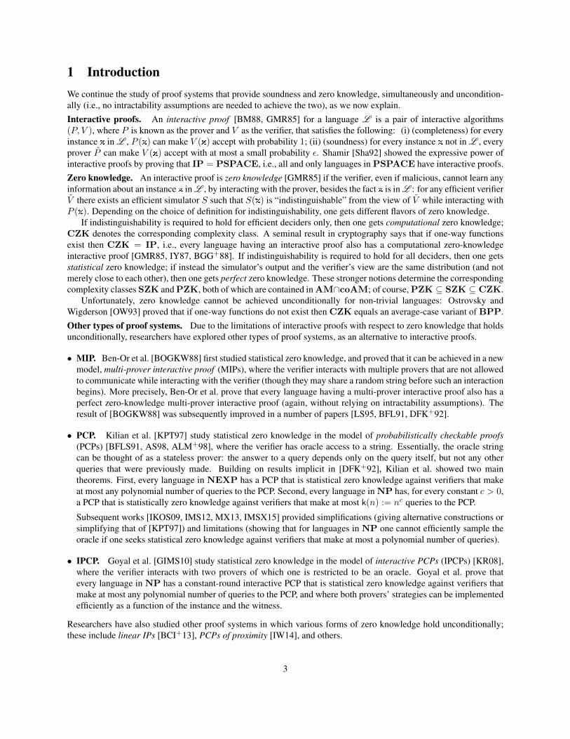
1 IntroductionWe continue the study of proof systems that provide soundness and zero knowledge, simultaneously and uncondition-ally (i.e., no intractability assumptions are needed to achieve the two), as we now explain.Interactive proofs. An interactive proof [BM88, GMR85] for a language L is a pair of interactive algorithms(P, V ), where P is known as the prover and V as the verifier, that satisfies the following: (i) (completeness) for everyinstance x in L , P (x) can make V (x) accept with probability 1; (ii) (soundness) for every instance x not in L , everyprover P can make V (x) accept with at most a small probability ε. Shamir [Sha92] showed the expressive power ofinteractive proofs by proving that IP = PSPACE, i.e., all and only languages in PSPACE have interactive proofs.Zero knowledge. An interactive proof is zero knowledge [GMR85] if the verifier, even if malicious, cannot learn anyinformation about an instance x in L , by interacting with the prover, besides the fact x is in L : for any efficient verifierV there exists an efficient simulator S such that S(x) is “indistinguishable” from the view of V while interacting withP (x). Depending on the choice of definition for indistinguishability, one gets different flavors of zero knowledge.

If indistinguishability is required to hold for efficient deciders only, then one gets computational zero knowledge;CZK denotes the corresponding complexity class. A seminal result in cryptography says that if one-way functionsexist then CZK = IP, i.e., every language having an interactive proof also has a computational zero-knowledgeinteractive proof [GMR85, IY87, BGG+88]. If indistinguishability is required to hold for all deciders, then one getsstatistical zero knowledge; if instead the simulator’s output and the verifier’s view are the same distribution (and notmerely close to each other), then one gets perfect zero knowledge. These stronger notions determine the correspondingcomplexity classes SZK and PZK, both of which are contained in AM∩coAM; of course, PZK ⊆ SZK ⊆ CZK.

Unfortunately, zero knowledge cannot be achieved unconditionally for non-trivial languages: Ostrovsky andWigderson [OW93] proved that if one-way functions do not exist then CZK equals an average-case variant of BPP.Other types of proof systems. Due to the limitations of interactive proofs with respect to zero knowledge that holdsunconditionally, researchers have explored other types of proof systems, as an alternative to interactive proofs.

• MIP. Ben-Or et al. [BOGKW88] first studied statistical zero knowledge, and proved that it can be achieved in a newmodel, multi-prover interactive proof (MIPs), where the verifier interacts with multiple provers that are not allowedto communicate while interacting with the verifier (though they may share a random string before such an interactionbegins). More precisely, Ben-Or et al. prove that every language having a multi-prover interactive proof also has aperfect zero-knowledge multi-prover interactive proof (again, without relying on intractability assumptions). Theresult of [BOGKW88] was subsequently improved in a number of papers [LS95, BFL91, DFK+92].

• PCP. Kilian et al. [KPT97] study statistical zero knowledge in the model of probabilistically checkable proofs(PCPs) [BFLS91, AS98, ALM+98], where the verifier has oracle access to a string. Essentially, the oracle stringcan be thought of as a stateless prover: the answer to a query depends only on the query itself, but not any otherqueries that were previously made. Building on results implicit in [DFK+92], Kilian et al. showed two maintheorems. First, every language in NEXP has a PCP that is statistical zero knowledge against verifiers that makeat most any polynomial number of queries to the PCP. Second, every language in NP has, for every constant c > 0,a PCP that is statistically zero knowledge against verifiers that make at most k(n) := nc queries to the PCP.

Subsequent works [IKOS09, IMS12, MX13, IMSX15] provided simplifications (giving alternative constructions orsimplifying that of [KPT97]) and limitations (showing that for languages in NP one cannot efficiently sample theoracle if one seeks statistical zero knowledge against verifiers that make at most a polynomial number of queries).

• IPCP. Goyal et al. [GIMS10] study statistical zero knowledge in the model of interactive PCPs (IPCPs) [KR08],where the verifier interacts with two provers of which one is restricted to be an oracle. Goyal et al. prove thatevery language in NP has a constant-round interactive PCP that is statistical zero knowledge against verifiers thatmake at most any polynomial number of queries to the PCP, and where both provers’ strategies can be implementedefficiently as a function of the instance and the witness.

Researchers have also studied other proof systems in which various forms of zero knowledge hold unconditionally;these include linear IPs [BCI+13], PCPs of proximity [IW14], and others.

3

A limitation of prior work. PCPs with quasilinear-size proof length, but without zero knowledge, are known:for every language L in NTIME(T (n)), there is a PCP with proof length O(T (n)) and query complexity O(1)[Din07, BS08, BGH+06, Mie08]. On the other hand, no such result for statistical zero knowledge PCPs is known:even when applied to PCPs of length O(T (n)), [KPT97]’s result and followup improvements yields a proof lengththat is polynomial in T (n) · k(n), where k(n), known as the knowledge bound, is a bound on the number of queriesby any verifier (see Section 4.1 for further discussion). We thus ask the following question: are there statistical zeroknowledge PCPs with proof length quasilinear in T (n) + k(n)?

1.1 Our contributionsWe do not answer the above question in the PCP model, but we give a positive answer in a closely related model thatcan be thought of as a “2-round PCP”, which we call duplex PCP (DPCP). At a high level, a DPCP works as follows:the prover first sends an oracle string π0 to the verifier, just as in a PCP; then, the verifier sends a message ρ to theprover; finally, the prover answers with a second oracle string π1; the verifier may query both oracles, and then acceptor reject. Thus, a DPCP is a special case of an interactive oracle proof (also known as a probabilistically checkableinteractive proof ) [BCS16, BCG+16, RRR16], which is an interactive proof in which the prover sends oracle stringsrather than messages. We prove the following theorem:

Theorem 1.1 (see Theorem 4.1 for formal statement). For every language L in NTIME(T )∩NP and polynomially-bounded knowledge bound k there exists a DPCP system satisfying the following:• the proof length (in fact, also the prover running time) is quasilinear in n+ T (n) + k(n);• the query complexity is polynomial in log(T (n) + k(n));• the verifier running time is polynomial in n+ log(T (n) + k(n));• perfect zero knowledge holds against any verifier that makes at most k(n) adaptive queries (in total to both oracles);• the soundness error is 1/2 (and can be reduced by repetition to 2−λ while preserving perfect zero knowledge,

provided that the number of queries does not exceed k(n)).

Moreover, similarly to the PCPs of [KPT97], the DPCP system that we construct is in fact not only sound but isalso a proof of knowledge [BG93]; however, in contrast to [KPT97], the DPCP verifier is non-adaptive, in the sensethat the query locations depend only on the verifier’s random tape.

Perhaps the main difference between our construction and prior work is the techniques that we use. While previousworks use the PCP Theorem as a black box, compiling a PCP into a zero knowledge PCP by using locking schemes[KPT97], we use certain algebraic properties of a specific family of PCPs to guarantee zero knowledge. In comparisonto the generic approach, we are more specific, but the addition of zero knowledge essentially comes “for free” whencompared to the corresponding constructions without zero knowledge. (In contrast, [KPT97] achieves a proof lengthof Ω(k(n)6 · l(n)c), for some large enough c, when starting from a PCP with proof length l(n).)DPCP vs IPCP. Duplex PCPs are an alternative to interactive PCPs that combine PCPs and interaction. In a DPCP,the verifier gets an oracle string from the prover, replies with a message, and then gets another oracle string from theprover; in an IPCP, the verifier gets an oracle string from the prover, and then engages in an interactive proof with him.

Both [GIMS10] and our work are similar in that both address aspects that we do not not know how to address inthe PCP model, and resort to studying alternative models, i.e., IPCP and DPCP respectively. The two works howevergive different flavors of results: [GIMS10] obtain IPCPs that are zero knowledge against verifiers that ask at most anypolynomial number of queries k(n) but their oracle is of polynomial size in k(n) (actually, of exponential size but witha polynomial-size circuit describing it); on the other hand, our work obtains DPCPs that are zero knowledge againstverifiers that ask at most a fixed polynomial number of queries k(n) and our oracles are of quasilinear size in k(n).

Finally, we note that our construction can be also cast as an IPCP, because the knowledge bound k(n) holds onlyfor the first oracle, i.e., perfect zero knowledge is preserved even if the verifier reads the second oracle in full. Thisprovides a result on a 2-round IPCP incomparable to [GIMS10]’s 4-round IPCP.On the minimal computational gap between prover and verifier needed for zero knowledge. IPs and MIPsassume a computational gap between prover and verifier. The prover is allowed (and often assumed) to be compu-tationally unbounded and the verifier is polynomially bounded. An intriguing corollary of our theorem is that thecomputational gap between prover and verifier can be drastically reduced, to a mere polylogarithmic one. Namely,

4

suppose that we wish to create zero-knowledge proof systems in which the verifier runs in time tv(n); in the modelabove, as long as tp(n) > tv(n) · (log tv(n))c for an absolute constant c, then perfect zero knowledge with a smallsoundness error can be obtained under no intractability assumptions. (See Corollary 4.2 for a formal statement.)

1.2 Open questionsThe duplex PCP model generalizes the PCP model. For which goals is this more powerful model necessary? Forexample, we have shown a construction of a duplex PCP with: (i) perfect zero knowledge with knowledge boundk(n); (ii) proof length O(T (n) + k(n)); and (iii) a non-adaptive verifier. In contrast, we do not know of PCPs thatachieve any one of these properties alone, while also maintaining unconditional zero knowledge. The work of Ishai,Weiss, and Yang [IWY16] obtains computational zero-knowledge PCPs with non-adaptive verifiers, using techniquesthat differ from both prior works on zero-knowledge PCPs and from ours; perhaps such techniques may lead to insightson the gap between duplex PCPs and PCPs.

Another intriguing open question concerns our main theorem (see Theorem 1.1), which only applies to languagesin NP, rather than all of NEXP. This limitation is due to an inefficiency of the simulator (see discussion of the timecomplexity of the simulator at the end of Section 6), but we do not know if the limitation is inherent.

5

2 Preliminaries

Functions and distributions. We use f : D → R to denote a function with domain D and range R; given a subsetD of D, we use f |D to denote the restriction of f to D. Given a distribution D, we write x ← D to denote that x issampled according to D.Distances. A distance measure is a function ∆: Σn × Σn → [0, 1] such that for all x, y, z ∈ Σn: (i) ∆(x, x) = 0,(ii) ∆(x, y) = ∆(y, x), and (iii) ∆(x, y) ≤ ∆(x, z) + ∆(z, y). For example, the relative Hamming distance overalphabet Σ is a distance measure: ∆Ham

Σ (x, y) := |i |xi 6= yi|/n. We extend ∆ to distances of strings to sets: givenx ∈ Σn and S ⊆ Σn, we define ∆(x, S) := miny∈S ∆(x, y) (or 1 if S is empty). We say that a string x is ε-close toanother string y if ∆(x, y) ≤ ε, and ε-far from y if ∆(x, y) > ε; similar terminology applies for a string x and a set S.Fields and polynomials. We denote by F a finite field, by Fq the field of size q, and by F the set of all finite fields.We denote by F[X1, . . . , Xm] the ring of polynomials inm variables over F; given a polynomial P in F[X1, . . . , Xm],degXi(P ) is the degree of P in the variable Xi; the total degree of P is the sum of all of these individual degrees. Forany set S ⊆ F let ZS(X) be the unique monic polynomial of degree |S| that vanishes on S: ZS(X) :=

∏α∈S(X−α).

Linear spaces. Given n ∈ N, a subset S of Fn is an F-linear space if αx+ βy ∈ S for all α, β ∈ F and x, y ∈ S.Languages and relations. We denote by R a relation consisting of pairs (x,w), where x is the instance and w is thewitness. We denote by Lan(R) the language corresponding to R, and by R|x the set of witnesses in R for x.Complexity classes. We write complexity classes in bold capital letters: NP, PSPACE, NEXP, and so on.We take a “relation-centric” point of view: we view NTIME as a class of relations rather than as the class of thecorresponding languages; we thus may write things like “let R be in NP”. If R is in NTIME(T ), we fix an arbitrarymachine MR that decides R in time T (n), i.e., MR(x,w) always halts after T (|x|) steps and MR(x,w) = 1 if andonly if (x,w) ∈ R; we then say that MR decides R (or Lan(R)). Throughout, we assume that T (n) ≥ n.Codes. An error correcting code C is a set of functions w : H → Σ, where H,Σ are finite sets. The messagelength of C is n := log|Σ| |C|, its block length is ` := |H|, its rate is ρ := n/`, its (minimum) distance is d :=min∆(w, z) |w, z ∈ C , w 6= z when ∆ is the (absolute) Hamming distance, and its (minimum) relative distanceis δ := d/`. Given a code family C , we denote by Rel(C ) the relation that naturally corresponds to C , i.e., (C,w) |C ∈ C , w ∈ C. A code C is linear if Σ is a finite field and C is a Σ-linear space in Σ`; we denote by dim(C)the dimension of C when viewed as a linear space. A code C is t-wise independent if, for every subset I of [`] withcardinality t, the distribution of w|I (viewed as a string) for a random w ∈ C equals the uniform distribution on Σt.Random shifts. We later use the following folklore claim about distance preservation for random shifts in linearspaces; for completeness, we include its short proof.

Claim 2.1. Let n be in N, F a finite field, S an F-linear space in Fn, and x, y ∈ Fn. If x is ε-far from S, then αx+ yis ε/2-far from S, with probability 1− |F|−1 over a random α ∈ F. (Distances are relative Hamming distances.)

Proof. Suppose, by way of contradiction, that there exist α1, α2 ∈ F and y1, y2 ∈ S with α1 6= α2 such that, for everyi ∈ 1, 2, αix+y is ε/2 close to yi. Then, by the triangle inequality, z := y1−y2 is ε-close to (α1x+y)−(α2x+y) =(α1 − α2)x. We conclude that x is ε-close to 1

α1−α2z ∈ S, a contradiction.

2.1 Probabilistically checkable proofsA PCP system [BFLS91, AS98, ALM+98] for a relation R is a tuple PCP = (P, V ) that works as follows.

• The prover P is a probabilistic algorithm that, given as input an instance-witness pair (x,w) with n := |x|, outputsa proof π : D(n)→ Σ(n), where both D(n) and Σ(n) are finite sets.

• The verifier V is a probabilistic oracle algorithm that, given as input an instance x with n := |x| and with oracleaccess to a proof π : D(n)→ Σ(n), queries π at a few locations and then outputs a bit.

The system PCP has (perfect) completeness and soundness error e(n) if the following two conditions hold. (Below,we explicitly denote the prover’s and verifier’s randomness as rP and rV .)

6

Completeness: For every instance-witness pair (x,w) in the relation R, PrrP ,rV[V P (x,w;rP )(x; rV ) = 1

]= 1 .

Soundness: For every instance x not in the language Lan(R) and proof π : D(n)→ Σ(n), PrrV [V π(x; rV ) = 1] ≤ e(n) .

A relation R belongs to the complexity class PCP[a, l, q, e, tp, tv] if there is a PCP system for R in which:– the answer alphabet (i.e., Σ(n)) is a(n),– the proof length over that alphabet (i.e., |D(n)|) is at most l(n),– the verifier queries the proof in at most q(n) locations,– the soundness error is e(n),– the prover runs in time tp(n), and– the verifier runs in time tv(n).Finally, we write na = Yes in the square brackets if the queries to the oracles are non-adaptive (i.e., the queriedlocations only depend on the verifier’s inputs); otherwise we write na = No.

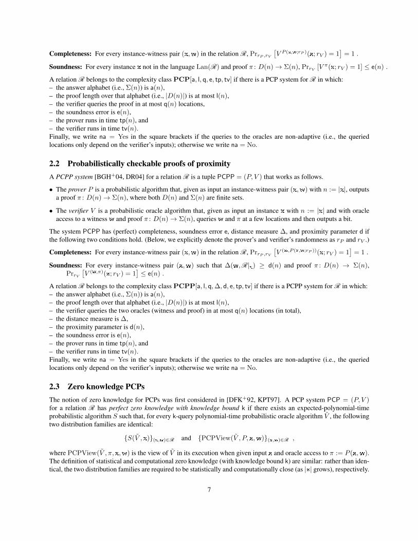
2.2 Probabilistically checkable proofs of proximityA PCPP system [BGH+04, DR04] for a relation R is a tuple PCPP = (P, V ) that works as follows.

• The prover P is a probabilistic algorithm that, given as input an instance-witness pair (x,w) with n := |x|, outputsa proof π : D(n)→ Σ(n), where both D(n) and Σ(n) are finite sets.

• The verifier V is a probabilistic oracle algorithm that, given as input an instance x with n := |x| and with oracleaccess to a witness w and proof π : D(n)→ Σ(n), queries w and π at a few locations and then outputs a bit.

The system PCPP has (perfect) completeness, soundness error e, distance measure ∆, and proximity parameter d ifthe following two conditions hold. (Below, we explicitly denote the prover’s and verifier’s randomness as rP and rV .)

Completeness: For every instance-witness pair (x,w) in the relation R, PrrP ,rV[V (w,P (x,w;rP ))(x; rV ) = 1

]= 1 .

Soundness: For every instance-witness pair (x,w) such that ∆(w,R|x) ≥ d(n) and proof π : D(n) → Σ(n),PrrV

[V (w,π)(x; rV ) = 1

]≤ e(n) .

A relation R belongs to the complexity class PCPP[a, l, q,∆, d, e, tp, tv] if there is a PCPP system for R in which:– the answer alphabet (i.e., Σ(n)) is a(n),– the proof length over that alphabet (i.e., |D(n)|) is at most l(n),– the verifier queries the two oracles (witness and proof) in at most q(n) locations (in total),– the distance measure is ∆,– the proximity parameter is d(n),– the soundness error is e(n),– the prover runs in time tp(n), and– the verifier runs in time tv(n).Finally, we write na = Yes in the square brackets if the queries to the oracles are non-adaptive (i.e., the queriedlocations only depend on the verifier’s inputs); otherwise we write na = No.

2.3 Zero knowledge PCPsThe notion of zero knowledge for PCPs was first considered in [DFK+92, KPT97]. A PCP system PCP = (P, V )for a relation R has perfect zero knowledge with knowledge bound k if there exists an expected-polynomial-timeprobabilistic algorithm S such that, for every k-query polynomial-time probabilistic oracle algorithm V , the followingtwo distribution families are identical:

S(V , x)(x,w)∈R and PCPView(V , P, x,w)(x,w)∈R ,

where PCPView(V , π, x,w) is the view of V in its execution when given input x and oracle access to π := P (x,w).The definition of statistical and computational zero knowledge (with knowledge bound k) are similar: rather than iden-tical, the two distribution families are required to be statistically and computationally close (as |x| grows), respectively.

7

A relation R belongs to the complexity class PCPpzk[a, l, q, e, tp, tv, k] if there exists a PCP system for R that(i) puts R in PCP[a, l, q, e, tp, tv], and (ii) has perfect zero knowledge with knowledge bound k; as for PCP, we addthe symbol na in the square brackets of PCPpzk to denote if the queries to the proof are non-adaptive. The complexityclasses PCPszk and PCPczk are similarly defined for statistical and computational zero knowledge.The KPT result. Kilian, Petrank, and Tardos proved the following theorem:

Theorem 2.2 ([KPT97]). For every polynomial time function T : N → N, polynomial security function λ : N → N,and polynomial knowledge bound function k : N→ N,

NTIME(T ) ⊆ PCPszk

answer alphabet a = F2poly(λ)

proof length l = poly(T, k)query complexity q = poly(λ)soundness error e = 2−λ

prover time tp = poly(λ, T )verifier time tv = poly(λ, T, k)knowledge bound knon-adaptive queries na = No

.

Remark 2.3. We make two remarks: (i) na = No because [KPT97]’s construction relies on adaptively querying theproof; (ii) inspection of [KPT97]’s construction reveals that l(n) ≥ poly(T (n)) · k(n)6.

2.4 Reed–Muller and Reed–Solomon codesWe define Reed–Muller and Reed–Solomon codes, as well as their “vanishing” variants [BS08]; all of these are linearcodes. We then state a theorem about PCPPs for certain families of RS codes.RM codes. Let F be a finite field, H,V subsets of F, m a positive integer, and % a constant in (0, 1]; % is calledthe fractional degree. The Reed–Muller code with parameters F, H,m, % is RM[F, H,m, %] := w : Hm → F |maxi∈[m] degXi(w) < %|H|; its message length is n = (%|H|)m, block length is ` = |H|m, rate is ρ = %m, and rela-tive distance is δ = 1− %. The vanishing Reed–Muller code with parameters F, H,m, %, V is VRM[F, H,m, %, V ] :=w ∈ RM[F, H,m, %] | w(V m) = 0; it is a subcode of RM[F, H,m, %]. We use the following folklore claim,whose correctness can be proved by induction on m:

Claim 2.4. Let F be a finite field, H,V subsets of F with H ∩V = ∅, m a positive integer, and t a positive integer notexceeding |H| − |V |. Then VRM[F, H,m, |V |+t|H| , V ] is t-wise independent.

RS codes. Let F be a finite field, H,V subsets of F, and % a constant in (0, 1]. The Reed–Solomon code withparameters F, H, % is RS[F, H, %] := RM[F, H, 1, %]. The vanishing Reed–Solomon code with parameters F, H, %, Vis VRS[F, H, %, V ] := w ∈ RS[F, H, %] | w(V ) = 0.Two RS code families and their PCPPs. Given `, χ : N→ N and % : N→ (0, 1), we denote by:• RS∗`,%,χ the set of Reed–Solomon codes RS[F, H, %] for which F has characteristic 2, H has cardinality at most `,

and the vanishing polynomial ZH is computable by a χ-size F-arithmetic circuit; and• VRS∗`,%,χ the set of vanishing Reed–Solomon codes VRS[F, H, %, V ] for which F has characteristic 2, H has car-

dinality at most `, and the vanishing polynomials ZH and ZV are computable by χ-size F-arithmetic circuits.The following theorem is from [BS08, BCGT13a] (the prover running time is shown in [BCGT13a] and the otherparameters in [BS08]).

8

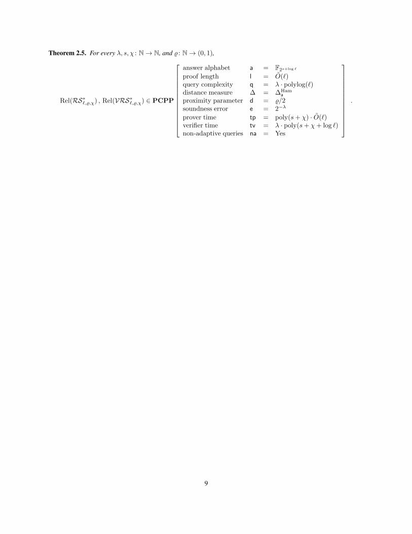
Theorem 2.5. For every λ, s, χ : N→ N, and % : N→ (0, 1),

Rel(RS∗`,%,χ) , Rel(VRS∗`,%,χ) ∈ PCPP

answer alphabet a = F2s+log `

proof length l = O(`)query complexity q = λ · polylog(`)distance measure ∆ = ∆Ham

a

proximity parameter d = %/2soundness error e = 2−λ

prover time tp = poly(s+ χ) · O(`)verifier time tv = λ · poly(s+ χ+ log `)non-adaptive queries na = Yes

.

9

3 Duplex PCPsWe define duplex PCPs, and then define notions of zero knowledge for this model. Our main theorem is the construc-tion of a duplex PCP with certain parameters; see Section 4. The difference between a PCP and a duplex PCP is thatall provers (both honest and malicious) produce two proof oracles rather than one: the prover produces a proof π0;then the verifier sends a message ρ to the prover; then the prover produces another proof π1; finally the verifier queriesboth π0 and π1 and either accepts or rejects. Thus, a PCP is a special case of a duplex PCP; in turn, a duplex PCP is aspecial case of an interactive oracle proof [BCS16, BCG+16, RRR16].

More precisely, a duplex PCP system for a relation R is a tuple DPCP = (P, V ) that works as follows.

• The prover P is a pair (P0, P1) of probabilistic algorithms, with shared randomness, where: (a) given as input aninstance-witness pair (x,w) with n := |x|, P0 outputs a proof π0 : D0(n)→ Σ(n); (b) given as input (x,w) and averifier’s message ρ (see below), P1 outputs a proof π1 : D1(n)→ Σ(n). Here D0(n), D1(n),Σ(n) are finite sets.

• The verifier V is a pair (V0, V1) of probabilistic algorithms, with shared randomness, where: (a) given as input aninstance xwith n := |x|, V0 outputs a message ρ; (b) given as input x and with oracle access to proofs π0 : D0(n)→Σ(n) and π1 : D1(n)→ Σ(n), V1 queries π0 and π1 at a few locations and then outputs a bit.

The system DPCP has (perfect) completeness and soundness error e(n) if the following two conditions hold. (Below,we explicitly denote the prover’s and verifier’s randomness as rP and rV .)

Completeness: For every instance-witness pair (x,w) in the relation R,

PrrP ,rV

V π0,π1

1 (x; rV ) = 1

∣∣∣∣∣∣π0 ← P0(x,w; rP )

ρ← V0(x; rV )π1 ← P1(x,w, ρ; rP )

= 1 .

Soundness: For every instance x not in the language Lan(R) and pair of algorithms P = (P0, P1),

PrrV

V π0,π1

1 (x; rV ) = 1

∣∣∣∣∣∣π0 ← P0

ρ← V0(x; rV )

π1 ← P1(ρ)

≤ e(n) .

A relation R belongs to the complexity class DPCP[a, l, q, e, tp, tv] if there is a DPCP system for R in which:– the answer alphabet (i.e., Σ(n)) is a(n),– the proof length over that alphabet (i.e., (|D0(n)|+ |D1(n)|)) is at most l(n),– the verifier queries the two proofs in at most q(n) locations (in total),– the soundness error is e(n),– the prover runs in time tp(n), and– the verifier runs in time tv(n).Finally, we write na = Yes in the square brackets if the queries to the oracles are non-adaptive (i.e., the queriedlocations only depend on the verifier’s inputs); otherwise we write na = No.Zero knowledge. A DPCP system DPCP = (P, V ) for a relation R has perfect zero knowledge with knowledgebound k if there exists an expected-polynomial-time probabilistic algorithm S such that for every pair of polynomial-time probabilistic oracle algorithms V := (V0, V1) the following two distribution families are identical:

S(V , x)(x,w)∈R and DPCPView(k, V , P, x,w)(x,w)∈R ,

where DPCPView(k, V , P, x,w) is the view of V1 in its execution when given input x and when allowed to makea total of k(n) adaptive queries to π0, π1, where π0 := P0(x,w) and π1 := P1(x,w, V π0

0 (x)). (As above, P0, P1

share the same randomness rP ; ditto for V0, V1.) The definition of statistical and computational zero knowledge (withknowledge bound k) are similar: rather than identical, the two distribution families are required to be statistically andcomputationally close (as |x| grows), respectively.

10

4 Main theoremThe main result of this paper is the following.

Theorem 4.1. For every polynomially-bounded time function T : N→ N and polynomially-bounded knowledge boundfunction k : N→ N with k ≤ T ,

NTIME(T ) ⊆ DPCPpzk

answer alphabet a = F2O(log(T+k))

proof length l = O(T + k)query complexity q = polylog(T + k)soundness error e = 1/2

prover time tp = poly(n) · O(T + k)verifier time tv = poly(n+ log(T + k))knowledge bound knon-adaptive queries na = Yes

.

The soundness error can be reduced from e = 1/2 to e = 2−λ via parallel repetition, with a corresponding λ-foldincrease in the query complexity q and verifier running time tv; perfect zero knowledge is preserved so long as thequery complexity does not exceed the knowledge bound k.A corollary. The above theorem says that, fixing T , the prover running time is quasilinear in the knowledge bound k,while the verifier running time is polylogarithmic in k. This yields an intriguing corollary: in the duplex PCP model,we only need a polylogarithmic computational overhead of the prover over the verifier in order to guarantee perfectzero knowledge. We state this formally next.

Corollary 4.2. For every polynomial time function T : N → N and relation R ∈ NTIME(T ), there is a constant csuch that, for every function tv : N→ N with tv(n) ≥ n · (log T (n))c, there is a DPCP system with:• completeness 1 and soundness 2−tv(n)/polylog(T (n));• perfect zero knowledge;• the verifier running time is tv(n) and prover running time is tp(n) := maxT (n)·(log T (n))c, tv(n)·(log tv(n))c.The verifier has no limitations other than a bound on its running time (its query complexity can be as large as tv(n)).

4.1 Proof sketchLet R be a relation in NP, and let (x,w) be an instance-witness pair in R. The prover and verifier both know x,while the prover also knows w. The prover wishes to convince the verifier that he knows a witness w for x, in such away that the verifier does not learn anything about w (beyond what can be inferred from the prover’s claim).The KPT approach. We introduce our ideas by contrasting them with those of [KPT97]. Suppose that the proverwishes to convince the verifier by sending him a PCP proof π = π(w) such that any k values in π do not revealanything about w. Loosely speaking, [KPT97] (building on [DFK+92]) provide a probabilistic transformation thatmaps the PCP proof π to a new proof π′, in which each bit of π is “hidden” amongst many bits of π′. The maintool employed in the transformation is a locking scheme, and its use imposes certain limitations: (i) the new proofπ′ is poly(k) larger than the original one (k6 by inspection of [DFK+92, KPT97]); (ii) zero knowledge holds onlystatistically, but not perfectly, because a malicious verifier can be “lucky” and obtain information on the bit of π beinglocked with fewer queries to π′ than expected.Our approach (ideally). We take a different approach: apply a “local” PCP to a “random” witness, as we nowexplain. Suppose that π = π(w) is (t, k)-local, i.e., any k positions of the PCP proof π jointly depend on at most tpositions of the witness w. Note that, even if π is (t, k)-local, a single bit of π can still leak information about w. Sosuppose further that the relation R is t-randomizable: given (x,w) ∈ R, one can efficiently sample a witnessw′ froma t-wise independent subset of the set of witnesses for x. In such a case, the prover can produce a zero-knowledgePCP as follows: (1) sample a witness w′ from the t-wise independent subset; then (2) send to the verifier the PCPproof π = π(w′). Indeed, the locality of π ensures that seeing any k indices of π reveals nothing about w, becausethese k indices are a function of t random bits. In sum, if we had a (t, k)-local PCP for a t-randomizable relation R,then we could obtain a PCP for R that is zero knowledge against verifiers that ask at most k queries.

11

Our approach (in reality). Unfortunately, we do not know how to obtain local PCPs for randomizable relations.However, we are able to obtain “partially local” duplex PCPs for certain randomizable relations, and also show thatNTIME can be efficiently reduced to these randomizable relations, as we now explain.

Our starting point are algebraic PCPs: certain PCPs that prove satisfiability of algebraic problems (APs) [PS94].Numerous known PCP constructions can be viewed as algebraic PCPs. Informally, in this work we make two basicobservations: (i) algebraic PCPs exist for certain randomizable relations; and (ii) an algebraic PCP proof can be splitin two parts, one part is local, while the other part is not local but enjoys convenient linear algebraic properties that,nevertheless, enable us to hide information about the witness, in the duplex PCP model. (Recall that, in the duplexPCP model, the prover produces a proof π0; then the verifier sends a message ρ to the prover; then the prover producesanother proof π1; finally the verifier queries both π0 and π1 and either accepts or rejects.)

In more detail, from a technical viewpoint, we proceed as follows. First, we introduce a family of constraintsatisfaction problems (CSPs) called linear algebraic CSPs, and show that NTIME is efficiently reducible to ran-domizable linear algebraic CSPs. The reduction consists of two parts: we go through an intermediary that we callgroup preserving algebraic problems (GAPs), a special case of APs that we believe to be of independent interest forthe study of algebraic PCPs. Second, we construct a duplex PCP system for randomizable linear algebraic CSPs thatis zero knowledge against verifiers that ask at most a certain number of queries.A technical piece: zero-knowledge duplex PCPP for low-degreeness. Later sections address all of the above steps(see Section 4.2 for a roadmap of these), and for now we only sketch one of these steps. Above we mention that analgebraic PCP proof has two parts: a local part, and a non-local part. This latter part of the proof arises from a centralcomponent of many PCP proofs: a PCP of proximity (PCPP) [BGH+05, DR04] that facilitates low-degree testing.Informally, given a function f : H → F and an integer d, a PCPP for degree d is a proof π(f) that f is ε-close to anevaluation of a polynomial degree at most degree d. We explain how to transform a PCPP for low-degreeness into aduplex PCPP for low-degreeness that is zero knowledge against verifiers that make at most t queries.

The set C of functions f : H → F that are evaluations of a polynomial of degree at most d is a subspace of F|H|.The basic idea is that, in order for the prover to convince the verifier that a function f is close to C, it suffices for theprover to convince the verifier that a random offset of f is close to C: one can verify that, for any u : H → F, if fis ε-far from C, then αf + u is ε/2-far from C, with probability 1 − |F|−1 over a random α ∈ F. Hence, we can letthe duplex PCP work as follows: (i) the prover samples a witness w′ from the t-wise independent subset, chooses arandom u ∈ C, and sends π0 := (w′, u) to the verifier; (ii) the verifier sends to the prover a random α ∈ F; (iii) theprover sends π1 = (v, π(v)) to the verifier, where v := αw′ + u and π(v) is a PCPP for low-degreeness of v; (iv) theverifier runs the PCPP verifier on (v, π) to check that v is close to C, and then checks that vi = αw′i + ui for a fewrandom indices i in 1, . . . , |H|.

Let us discuss the various properties of the duplex PCPP.• COMPLETENESS: If w ∈ C, then αw′ + u ∈ C; therefore, the prover convinces the verifier.• ZERO-KNOWLEDGE: If the verifier asks at most t queries, then he learns nothing about w because: π0 = (w′, u)

contains w′ sampled from a t-wise independent subset and u random in C; π1 = (v, π(v)) is running the PCPP ona vector v that is random in C.

• SOUNDNESS: If v does equal α ·w+ u, then the verifier rejects with high probability because v is far from C (andthe PCPP verifier rejects π with high probability). If instead v does not equal α ·w+ u, then the fact that v is closeto C does not prove anything about whether w is also close. So, in this case, we need to reason about the successprobability of the verifier’s linearity tests: if these pass with enough probability, then with high probability v is closeto αw + u, which again suffices for our purpose. Overall, soundness holds.

Next, we discuss how the technical sections are organized, and how they come together to yield our main theorem.

4.2 Roadmap of the rest of the paperThe rest of the paper is dedicated to turn the above intuition into a more formal proof. To do so, we introduce variousintermediate steps, as follows.• In Section 5, we introduce linear algebraic CSPs (a family of constraint satisfaction problems), and then describe

how to obtain a canonical PCP for any linear algebraic CSP.

12

• In Section 6, we introduce randomizable linear algebraic CSPs, a subfamily of linear algebraic CSPs; then we showthat, for every randomizable linear algebraic CSP, we can convert the CSP’s canonical PCP into a correspondingzero-knowledge duplex PCP, incurring only little overheads.

• In Section 7, we show an efficient reduction from NTIME to randomizable linear algebraic CSPs; along theway, we introduce a family of algebraic problems, having special symmetry properties, that we believe to be ofindependent interest (e.g., for studying other questions about PCPs).

Combining (i) the efficient reduction from NTIME to randomizable linear algebraic CSPs together with (ii) thezero-knowledge duplex PCP for such problems yields Theorem 4.1. In Section 8 we provide details about how thesecomponents are combined.

13

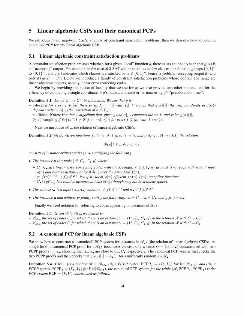
5 Linear algebraic CSPs and their canonical PCPsWe introduce linear algebraic CSPs, a family of constraint satisfaction problems; then we describe how to obtain acanonical PCP for any linear algebraic CSP.

5.1 Linear algebraic constraint satisfaction problemsA constraint satisfaction problem asks whether, for a given “local” function g, there exists an input α such that g(α) isan “accepting” output. For example, in the case of 3-SAT with n variables and m clauses, the function g maps 0, 1nto 0, 1m, and g(α) indicates which clauses are satisfied by α ∈ 0, 1n; hence α yields an accepting output if (andonly if) g(α) = 1m. Below we introduce a family of constraint satisfaction problems whose domain and range arelinear-algebraic objects, namely, linear error correcting codes.

We begin by providing the notion of locality that we use for g; we also provide two other notions, one for theefficiency of computing a single coordinate of g’s output, and another for measuring g’s “pseudorandomness”.

Definition 5.1. Let g : Σn → Σm be a function. We say that g is:– q-local if for every j ∈ [m] there exists Ij ⊆ [n] with |Ij | ≤ q such that g(α)[j] (the j-th coordinate of g(α))

depends only on α|Ij (the restriction of α to Ij);– c-efficient if there is a time c algorithm that, given j and α|Ij , computes the set Ij and value g(α)[j];– (γ, ε)-sampling if Pr[ Ij ∩ I 6= ∅ | j ← [m] ] ≤ γ for every I ⊆ [n] with |I|/n ≤ ε.

Next we introduce RLA, the relation of linear algebraic CSPs:

Definition 5.2 (RLA). Given functions f : N→ F , `, q, c : N→ N, and ρ, δ, γ, ε : N→ (0, 1], the relation

RLA[f, `, ρ, δ, q, c, γ, ε]

consists of instance-witness pairs (x,w) satisfying the following.

• The instance x is a tuple (1n, C, C•, g) where:

– C, C• are linear error correcting codes with block lengths `(n), `•(n) at most `(n), each with rate at mostρ(n) and relative distance at least δ(n) over the same field f(n);

– g : f(n)`(n) → f(n)`•(n) is a q(n)-local, c(n)-efficient, (γ(n), ε(n))-sampling function;– C• ∪ g(C) has relative distance at least δ(n) (though may not be a linear space).

• The witness w is a tuple (α, α•) where α ∈ f(n)`(n) and α• ∈ f(n)`•(n).

• The instance x and witness w jointly satisfy the following: α ∈ C, α• ∈ C•, and g(α) = α•.

Finally we need notation for referring to codes appearing in instances of RLA:

Definition 5.3. Given R ⊆ RLA, we denote by– CR, the set of codes C for which there is an instance x = (1n, C, C•, g) in the relation R with C = C;– CR,• the set of codes C for which there is an instance x = (1n, C, C•, g) in the relation R with C = C•.

5.2 A canonical PCP for linear algebraic CSPsWe show how to construct a “canonical” PCP system for instances in RLA (the relation of linear algebraic CSPs). Ata high level, a canonical PCP proof for a RLA-instance x consists of a witness w = (α, α•) concatenated with twoPCPP proofs π, π•, showing that α, α• are close to C, C• respectively. The canonical PCP verifier first checks thetwo PCPP proofs and then checks that g(α)[j] = α•[j] for a uniformly random j ∈ [`•].

Definition 5.4. Given (i) a relation R ⊆ RLA, (ii) a PCPP system PCPP = (P, V) for Rel(CR,), and (iii) aPCPP system PCPP• = (P•, V•) for Rel(CR,•), the canonical PCP system for the triple (R,PCPP,PCPP•) is thePCP system PCP = (P, V ) constructed as follows.

14

• Prover. Given (x,w) ∈ RLA, the PCP prover P outputs π := (w, π, π•) where π := P(C, α) and π• :=P•(C•, α•). In other words, the PCP prover outputs a PCP proof that is the concatenation of the witness w =(α, α•) and a pair of PCPP proofs, the first proving that α ∈ C and the second proving that α• ∈ C•.

• Verifier. Given x and oracle access to a PCP proof π = (w, π, π•), the PCP verifier V works as follows:

– (proximity) check that V (α,π) (C) and V (α•,π•)

• (C•) both accept;– (consistency) check that g(α)[j] = α•[j] for a uniformly random j ∈ [`•].

The next lemma says that the above construction is a PCP system when RLA’s parameters are sufficiently “good”.

Lemma 5.5 (RLA → PCP). Suppose that R is a relation that satisfies the following conditions:(i) R ⊆ RLA[f1, `1, ρ1, δ1, q1, c1, γ1, ε1] with ε1 < min δ12 , δ1 − γ1;

(ii) Rel(CR,),Rel(CR,•) ∈ PCPP[a2, l2, q2,∆Hama2

, d2, e2, tp2, tv2, na2] with a2 = f1 and d2 ≤ ε1.Then there is a canonical PCP system for a triple (R,PCPP,PCPP•) that yields

R ∈ PCP

answer alphabet a = f1 (= a2)proof length l = 2l2(`1) + 2`1query complexity q = 2q2(`1) + q1 + 1soundness error e = max1− δ1 + γ1 + ε1, e2prover time tp = 2tp2(`1)verifier time tv = 2tv2(`1) + c1 + log `1non-adaptive queries na = na2

.

Proof of Lemma 5.5. First, we show that the canonical PCP system satisfies completeness and soundness; afterwards,we discuss the efficiency parameters achieved by it.Completeness. Consider an instance-witness pair (x,w) in the relation R. Parse the instance x as (1n, C, C•, g)and the witness w as (α, α•). Since (x,w) ∈ R, we have that α ∈ C, α• ∈ C•, and g(α) = α•. Therefore,the PCP proof (w, π, π•) generated by the PCP prover is accepted by the PCP verifier with probability 1: the PCPPverifiers V (α,π)

(C) and V (α•,π•)• (C•) always accept and g(α)[j] = α•[j] for every j ∈ [`•].

Soundness. Consider an instance x not in the language Lan(R) and a PCP proof π = (w, π, π•). Parse the instancex as (1n, C, C•, g) and the wintess w, inside π, as (α, α•). We prove that V accepts π with probability at mostmax1− δ1 + γ + ε1, e2, by considering the following three cases.

• Case 1: α is ε1-far in relative Hamming distance from C. The canonical PCP verifier’s proximity test fails,because ∆Ham

a (α, C) ≥ ε1 ≥ d2, and so the PCPP verifier V (α,π) (C) accepts with probability at most e2.

• Case 2: α• is ε1-far in relative Hamming distance from C•. This case is analogous to the previous one.

• Case 3: there exist α ∈ C and α• ∈ C• with ∆Hama (α, α) ≤ ε1 and ∆Ham

a (α•, α•) ≤ ε1.

First, since ε1 is less than δ1/2 (the unique decoding radius of C and C•), the codewords α and α• are unique.

Next, we claim that α′• := g(α) and g(α) are γ1-close. Indeed, since g is (γ1, ε1)-sampling, α and α differ inat most ε1 · `(n) positions, and so at most γ1 · `•(n) positions of g(α) depend on an index where α and α differ.

Next, we claim that ∆Hama (α•, α

′•) ≥ δ1. Indeed, we have that α• 6= α′• because otherwise (α, α•) would be a

satisfying assignment for x (contradicting the assumption that x 6∈ Lan(R)); moreover, we also have thatC•∪g(C)has relative distance at least δ1.

We now use the triangle inequality, along with the above observations, to obtain that

δ1 ≤ ∆Hama (α•, α

′•)

≤ ∆Hama (α•, α•) + ∆Ham

a (α•, g(α)) + ∆Hama (g(α), α

′•)

≤ ε1 + ∆Hama (α•, g(α)) + γ1 .

Thus, ∆Hama (α•, g(α)) ≥ δ1 − (γ1 + ε1), and so the canonical PCP verifier’s consistency check passes with

probability at most 1− δ1 + γ1 + ε1.

15

We conclude that V accepts π with probability at most max1− δ1 + γ1 + ε1, e2.Other parameters. The remaining parameters are straightforward to establish. The canonical PCP does not changethe alphabet, so a = f1 (which also equals a2). The proof length, and the running times of the prover and verifier arethe sum of the same measures of the sub-components: the PCP proof has l = 2l2(`1) + 2`1 symbols, is produced intime tp = 2tp2(`1), and is verified in time tv = 2tv2(`1)+c1 +O(1). The canonical PCP verifier makes q1 +1 querieson top of those of the PCPP verifiers, so its query complexity is q = 2q2(`1) + q1 + 1. The q1 + 1 additional queriesare non-adaptive; so if the PCPP verifiers are non-adaptive, so is the canonical PCP verifier (i.e., na = na2).

16

6 Zero-knowledge duplex PCPs from randomizable linear algebraic CSPsWe introduce randomizable linear algebraic CSPs, a subfamily of linear algebraic CSPs. Then we show that, for everyrandomizable linear algebraic CSP, we can convert the CSP’s canonical PCP into a corresponding zero-knowledgeduplex PCP, incurring only little overheads.

6.1 Randomizable linear algebraic CSPsThe definition below specifies the notion of randomizability for linear algebraic CSPs.

Definition 6.1 (RRLA). The relation RRLA[f, `, ρ, δ, q, c, γ, ε, t, r] is the sub-relation of RLA[f, `, ρ, δ, q, c, γ, ε] ob-tained by restricting it to instances that are t-randomizable in time r. An instance x = (1n, C, C•, g) is t(n)-randomizable in time r(n) if: (i) there exists a t(n)-wise independent subcode C ′ ⊆ C such that if (w, g(w))satisfies x, then, for every w′ in C ′ + w := w′ + w | w′ ∈ C ′, the witness (w′, g(w′)) satisfies x; and (ii) onecan sample, in time r(n), three uniformly random elements in C ′, C and C• respectively.

Remark 6.2. A linear code C ⊆ F` is t-wise independent if and only if its dual distance is at least t, i.e., its dual codeC⊥ := w ∈ F` | ∀z ∈ C,

∑`i=1 wizi = 0 has distance at least t.

Remark 6.3. A random codeword in a linear code C ⊆ F` can be sampled with r := ` · dim(C) field operations inF, by using a generating matrix for C. In certain cases, a random codeword can be sampled more efficiently; e.g., inthe case of Reed–Muller codes, ` · polylog(dim(C)) field operations are sufficient (via a suitable use of FFTs).

6.2 Construction of zero-knowledge duplex PCPsWe construct a zero-knowledge duplex PCP system for randomizable linear algebraic CSPs. The duplex PCP systemdoes little more than invoking, as a subroutine, the canonical PCP system for the linear algebraic CSP; hence, theefficiency of the duplex PCP and of the canonical PCP system are closely related. The construction demonstrates that“adding zero knowledge to an algebraic PCP” is cheap, provided that one moves from the PCP model to the (moregeneral) duplex PCP model. More precisely, we prove the following theorem.

Theorem 6.4 (RRLA → DPCPpzk). Suppose that R is a relation that satisfies the following conditions:(i) R ⊆ RRLA[f1, `1, ρ1, δ1, q1, c1, γ1, ε1, t1, r1] with ε1 < min δ12 , δ1− γ1 and `1, c1, r1 polynomially bounded;

(ii) Rel(CR,),Rel(CR,•) ∈ PCPP[a2, l2, q2,∆Hama2

, d2, e2, tp2, tv2, na2] with a2 = f1 and d2 ≤ ε1/4.Then there is a duplex PCP system for R that yields

R ∈ DPCPpzk

answer alphabet a = f1 (= a2)proof length l = 2l2(`1) + 6`1query complexity q = 2q2(`1) + q1 + 7soundness error e = max1− δ1 + γ1 + ε1 , (1− |f1|−1) ·maxe2, ε1/4+ |f1|−1prover time tp = 2tp2(`1) + (c1 + 5)`1 + r1

verifier time tv = 2tv2(`1) + c1 + log `1knowledge bound k = t1/q1

non-adaptive queries na = na2

.

Proof. We prove the claim by constructing a suitable duplex PCP system DPCP = (P, V ) for the relation R. Recallthat: the prover P is a pair of algorithms (P0, P1), and the verifier V is also a pair of algorithms (V0, V1); moreover, aninstance x of R is of the form (1n, C, C•, g), while a witness w of R is of the form (α, α•); finally, randomizabilityimplies that there is a t(n)-wise independent subcode C ′ ⊆ C such that if (w, g(w)) satisfies x then so does thewitness (w′, g(w′)), for every w′ in C ′ + w.

We now describe the construction of the duplex PCP system DPCP = (P, V ):

• P0(x,w)→ π0

Sample uniformly random v ∈ C, v• ∈ C•, u′ ∈ C ′; compute w := u′ + α, w• := g(w) and output

π0 := (w‖v‖w•‖v•).

17

• V0(x)→ ρ

Sample uniformly random ρ, ρ• ∈ f1, and output ρ := (ρ, ρ•).

• P1(x,w, ρ)→ π1

Compute z := ρw + v and z• := ρ•w• + v•; compute π := P(C, z) and π• = P•(C•, z•); and outputπ1 := (z‖z•‖π‖π•). (Essentially, this step corresponds to running the canonical PCP prover with respect to auniformly random pair (z, z•) in (C, C•).)

• V π0,π1

1 (x)→ b

Conduct the following tests (and reject if any of them fails):

– (proximity) check that V (z,π) (C) and V (z•,π•)

• (C•) both accept;– (consistency) check that g(w)[j] = w•[j] for a random j ∈ [`•];– (linearity) check that z[i] = ρw[i]+v[i] and z•[k] = ρ•w•[k]+v•[k] for random i ∈ [`(n)] and k ∈ [`•(n)].

(Essentially the first two steps correspond to running the canonical PCP verifier on modified inputs, while the thirdstep consists of two linearity tests.)

Having described the duplex PCP system, we now show that it satisfies completeness, soundness and zero-knowledge;afterwards, we discuss the efficiency parameters achieved by it.Completeness. Consider an instance-witness pair (x,w) in the relation R. Since (x,w) ∈ R, we have that α ∈ C,α• ∈ C•, and g(α) = α•. Sincew ∈ C ′+α and R is randomizable, we have that (w, w•) := (w, g(w)) satisfiesx; thus V1’s consistency check passes with probability 1. Since the codes C and C• are linear and w, v ∈ C,w•, v• ∈ C•, we have that z := ρw + v ∈ C and z• := ρ•w• + v• ∈ C•; thus the PCPP verifiers V (z,π)

(C)

and V (z•,π•)• (C•) accept with probability 1. Finally, by construction of z and z•, V1’s linearity tests also accept with

probability 1. We conclude that the duplex PCP system described above has perfect completeness.Soundness. Consider an instance x not in the language Lan(R). Fix an arbitrary proof string π0 = (w‖v‖w•‖v•),and let the proof string π1 = (z‖z•‖π‖π•) depend arbitrarily on the verifier message ρ = (ρ, ρ•). We prove thisby distinguishing between the three cases below.

• Case 1: w is ε1-far in relative Hamming distance from C.

Claim 2.1 implies that z′ := ρw+ v is ε1/2-far from C, with probability 1−|f1|−1 over a random choice of ρ.Let θ := ∆Ham

a (z′, z) and η := ∆Hama (z, C). By the triangle inequality, θ+ η ≥ ∆Ham

a (z′, C) ≥ ε1/2; hence,at least one of the inequalities θ ≥ ε1/4 and η ≥ ε1/4 holds. In the former case, V1’s first linearity test accepts withprobability at most 1 − ε1/4; in the latter case, the PCPP verifier V (z,π)

(C) for V1’s first proximity test acceptswith probability at most e2, as ∆Ham

a (z, C) ≥ ε1/4 ≥ d2.

• Case 2: w• is ε1-far in relative Hamming distance from C•.

This case is analogous to the previous one.

• Case 3: there exist w ∈ C and w• ∈ C• with ∆Hama (w, w) ≤ ε1 and ∆Ham

a (w•, w•) ≤ ε1.

In this case we follow the very end of the soundness analysis in Lemma 5.5’s proof, replacing α, α• there withw, w•, and conclude that the verifier accepts with probability at most 1− δ1 + γ1 + ε1.

Summing up, in the first case the verifier’s acceptance probability is at most (1 − |f1|−1) ·maxe2, ε1/4 + |f1|−1;similarly for the second case. In the third case the rejection probability is 1− δ1 + γ1 + ε1, that of the canonical PCPconsistency verifier. This completes the soundness analysis.Zero knowledge. We construct a simulator S that yields perfect zero knowledge with knowledge bound k. Consideran instance-witness pair (x,w) in the relation R, and a malicious verifier V = (V0, V1) making at most k adaptivequeries. The output of the simulator S when given as input V and x, denoted S(V , x), has to be identically distributedto DPCPView(k, V , P, x,w), which is the view of V1 in its execution when given input x and when allowed to makea total of k(n) adaptive queries to π0, π1, where π0 := P0(x,w) and π1 := P1(x,w, V π0

0 (x)). In fact, we will prove a

18

stronger statement: the output of the simulator continues to exactly match the view of the verifier, interacting with thehonest prover, even if the verifier is allowed unbounded access to π1, provided that V makes at most k queries to π0.

We now discuss how S works. At a high level, S treats V as a black box, running it once without rewinding; alongthe way, S samples suitable answers for each query (as discussed below); when V halts, S outputs all the answers andV ’s message (which together form the view of the verifier). The simulator S runs in strict polynomial time, withoutever aborting. We now describe how S answers each query.

The simulator S maintains a proof string πS = (πS0 , πS1 ) where πS0 = (wS , v

S , w

S• , v

S• ) and πS1 = (zS , z

S• , π

S , π

S• ).

Initially, πS is unspecified at all locations. The simulator maintains two sets,A ⊆ [`] andA• ⊆ [`•], that are initiallyempty. At any stage of the simulation, A and A• contain the set of indices of wS , v

S and wS• , v

S• that are currently

specified, respectively.We now discuss how S adaptively specifies locations in πS . We distinguish between two parts of the simulation:

before the point when V sends his message ρ, and only queries to π0 are possible; and afterwards, when queries toboth π0 and π1 are possible. When V requests an index j ∈ [`] of w or v that is unspecified, the simulator willupdate both wS and vS at j. The value vS [j] is set to a random field element, unless its value is already determined bypreviously specified indices together with the linear constraint that vS must be a projection of an element of C. Thisimplies that at any stage of the simulation, the specified part of vS is a projection of a uniform element of C. Duringthe first part of the simulation, wS [j] is simply updated to a random field element. During the second part, it is updatedaccording to the linear relation ρ · wS + vS = zS . The strings wS• and vS• are updated similarly. An important thingto note is that to update wS• [j] the simulator first queries all indices of wS on which wS• [j] depends. In more detail, thesimulator works as follows.

• Simulating answers to π0 = (w‖v‖w•‖v•), before V outputs ρ = (ρ, ρ•).

1. Initialize A := ∅, A• := ∅.2. For a query j ∈ [`] to either w[j] or v[j] with j /∈ A:

– Check if vS [j] is determined by a linear constraint of C together with the values vS [j′] | j′ ∈ A and,if so, update vS [j] to that value. Otherwise, update vS [j] to a random field element γ ∈ f1.

– Set wS [j] to a random field element β ∈ f1.– Add j to A.

3. For a query j ∈ [`•] to either w•[j] or v•[j] with j /∈ A•:– Check if vS• [j] is determined by a linear constraint of C• together with the values vS• [j′] | j′ ∈ A• and,

if so, update vS• [j] to that value. Otherwise, update vS• [j] to a random field element γ ∈ f1.– Do the following: (i) compute the set Ij ⊆ [`•] of locations on which g(wS )[j] depends (see Defini-

tion 5.2); (ii) deduce wS |Ij by querying each i ∈ Ij according to Step 2; and (iii) set wS• [j] := g(wS |Ij ).– Add j to A•.

• Simulating answers to π0 = (w‖v‖w•‖v•) and π1 = (z‖z•‖π‖π•), after V outputs ρ = (ρ, ρ•).

4. After receiving ρ = (ρ, ρ•), immediately do the following:(a) sample a random zS ∈ C under the constraint “zS [i] = ρw

S [i] + vS [i] for all i ∈ A”;

(b) sample a random zS• ∈ C• under the analogous constraint;(c) compute πS := P(C, z

S );

(d) compute πS• := P•(C•, zS• ).

5. All queries to z, z•, π, π• are answered according to the values specified in Step 4.6. For a query j ∈ [`] to either w[j] or v[j] with j /∈ A:

– Check if vS [j] is determined by a linear constraint of C together with the values vS [j′] | j′ ∈ A and,if so, update vS [j] to that value. Otherwise, update vS [j] to a random field element γ ∈ f1.

– If ρ = 0, set wS [j] uniformly at random, otherwise set wS [j] := (zS [j]− vS [j])/ρ.– Add j to A.

7. For a query j ∈ [`•] to either w•[j] or v•[j] with j /∈ A•:– Do the following: (i) compute the set Ij ⊆ [`•] of locations on which g(wS )[j] depends (see Defini-

tion 5.2); (ii) deduce wS |Ij by querying each i ∈ Ij according to Step 6; and (iii) set wS• [j] := g(wS |Ij ).

– Set vS• [j] := zS• [j]− ρ• · wS• [j].

19

– Add j to A•.

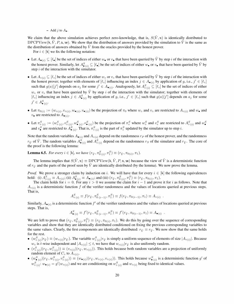
We claim that the above simulation achieves perfect zero-knowledge, that is, S(V , x) is identically distributed toDPCPView(k, V , P, x,w). We show that the distribution of answers provided by the simulation to V is the same asthe distribution of answers obtained by V from the oracles provided by the honest prover.

For i ∈ [k] we fix the following notation:

• Let A•(i) ⊆ [`•] be the set of indices of either w• or v• that have been queried by V by step i of the interaction withthe honest prover. Similarly, let AS• (i) ⊆ [`•] be the set of indices of either w• or v• that have been queried by V bystep i of the interaction with the simulator.

• Let A(i) ⊆ [`] be the set of indices of either w or v that have been queried by V by step i of the interaction withthe honest prover; together with elements of [`] influencing an index j ∈ A•(i) by application of g, i.e., j′ ∈ [`]

such that g(a)[j′] depends on aj for some j′ ∈ A•(i). Analogously, let AS (i) ⊆ [`] be the set of indices of eitherw or v that have been queried by V by step i of the interaction with the simulator; together with elements of[`] influencing an index j ∈ AS• (i) by application of g, i.e., j′ ∈ [`] such that g(a)[j′] depends on aj for somej′ ∈ AS• (i).

• Let π0(i) := (w(i), v(i), w•(i), v•(i)) be the projection of π0 where w and v are restricted to A(i) and w• andv• are restricted to A•(i).

• Let πS (i) := (wS (i), vS (i), w

S• (i), v

S• (i)) be the projection of πS where wS and vS are restricted to AS (i) and wS•

and vS• are restricted to AS• (i). That is, πS (i) is the part of πS updated by the simulator up to step i.

Note that the random variablesA•(i) andA(i) depend on the randomness rP of the honest prover, and the randomnessrV of V . The random variables AS• (i) and AS (i) depend on the randomness rS of the simulator and rV . The core ofthe proof is the following lemma:

Lemma 6.5. For every i ∈ [k], we have (rV , πS0 (i), π

S1 ) ≡ (rV , π0(i), π1).

The lemma implies that S(V , x) ≡ DPCPView(k, V , P, x,w) because the view of V is a deterministic functionof rV and the parts of the proof seen by V are identically distributed (by the lemma). We now prove the lemma.

Proof. We prove a stronger claim by induction on i. We will have that for every i ∈ [k] the following equivalenceshold: (i) AS (i) ≡ A(i); (ii) AS• (i) ≡ A•(i); and (iii) (rV , π

S0 (i), π

S1 ) ≡ (rV , π0(i), π1).

The claim holds for i = 0. For any i > 0 we assume the claim for i − 1 and prove it for i as follows. Note thatA(i) is a deterministic function f of the verifier randomness and the values of locations queried at previous steps.That is,

AS (i) ≡ f(rV , πS0 (i−1), π

S1 ) ≡ f(rV , π0(i−1), π1) ≡ A(i) .

Similarly,A•(i) is a deterministic function f ′ of the verifier randomness and the values of locations queried at previoussteps. That is,

AS• (i) ≡ f′(rV , π

S0 (i−1), π

S1 ) ≡ f ′(rV , π0(i−1), π1) ≡ A•(i) .

We are left to prove that (rV , πS0 (i), π

S1 ) ≡ (rV , π0(i), π1). We do this by going over the sequence of corresponding

variables and show that they are identically distributed conditioned on fixing the previous corresponding variables tothe same values. Clearly, the first components are identically distributed: rV ≡ rV . We now show that the same holdsfor the rest.• (wS (i)|rV ) ≡ (w(i)|rV ). The variable wS (i)|rV is simply a uniform sequence of elements of size |A(i)|. Becausew is t-wise independent and |A(i)| ≤ t, we have that w(i)|rV is also uniformly random.

• (vS (i)|(rV , wS (i))) ≡ (v(i)|(rV , w(i))). This holds because both random variables are a projection of uniformlyrandom element of C to A(i).

• (wS• (i)|(rV , wS (i), vS (i))) ≡ (w•(i)|(rV , w(i), v(i))). This holds because wS• (i) is a deterministic function g′ of

wS (i): w•(i) = g′(w(i)) and we are conditioning on wS (i) and w(i) being fixed to identical values.

20

• (vS• (i)|(rV , wS (i), vS (i), w

S• (i))) ≡ (v•(i)|(rV , w(i), v(i), w•(i))). This holds because both random variables are

a projection of uniformly random element of C• to A•(i).• (zS |(rV , wS (i), v

S (i), w

S• (i), v

S• (i))) ≡ (z|(rV , w(i), v(i), w•(i), v•(i))). This holds because both are a uniform

element a of C conditioned on ρ0 · w[j] + v[j] = a[j] for every j ∈ A(i).• (zS• |(rV , wS (i), v

S (i), w

S• (i), v

S• (i), z

S )) ≡ (z•|(rV , w(i), v(i), w•(i), v•(i), z)). This holds because both are a

uniform element a of C• conditioned on ρ1 · w•[j] + v•[j] = a[j] for every j ∈ A•(i).Recall that π0(i) = (w(i)‖v(i)‖w•(i)‖v•(i)) and π1 = (z‖z•‖π‖π•) and similarly for πS0 (i) and πS1 ; the abovethen implies that: (i) rV ≡ rV ; (ii) (πS0 (i)|rV ) ≡ (π0(i)|rV ); and (iii) (πS1 |(rV , πS0 (i))) ≡ (π1|(rV , π0(i))), that is,(rV , π

S0 (i), π

S1 ) ≡ (rV , π0(i), π1).

We conclude the discussion of the simulator by examining the time complexity of the simulation. Most steps of thesimulation require (a) sampling a random field element and, possibly, (b) solving a linear system with a polynomialnumber of equations. The only expensive part of the simulation is Step 4, because it requires sampling randomcodewords in C and C•, as well as computing PCPP proofs for these two codewords. Provided that `1, c1, r1 arepolynomially bounded, the entire simulation also runs in polynomial time in the instance size n. (The definition ofzero knowledge in Section 3 prescribes, as typically done, a simulator that runs in expected probabilistic polynomialtime; our simulator runs in strict probabilistic polynomial time.)Other parameters. The remaining parameters are straightforward to establish. The duplex PCP construction doesnot change the alphabet, so a = f1 (which also equals a2). The proof length, and the running times of the prover andverifier are the sum of the same measures of the duplex PCP’s components: the PCP proofs have l = 2l2(`1) + 6`1symbols in total, are produced in time tp = 2tp2(`1) + (c1 + 5)`1 + r1, and are verified in time tv = 2tv2(`1) +c1 + log `1. The duplex PCP verifier makes q1 + 7 queries on top of those made by the two PCPP verifiers, so itsquery complexity is q = 2q2(`1) + q1 + 7. The q1 + 7 additional queries are non-adaptive; so if the PCPP verifiersare non-adaptive, so is the duplex PCP verifier (i.e., na = na2).

Remark 6.6 (Necessity of duplex PCP). Claim 2.1 suggests a way to modify our duplex PCP construction so that theprover sends the oracle proof strings in one message (as in a standard PCP) rather than over two rounds of interaction.Namely, assuming w is ε-far from C, there is at most one verifier message ρ that makes z be ε/2-close to C.Hence the verifier can fix in advance r distinct ρ(1)

, . . . , ρ(r) and have the prover send, in addition to π0, the oracle

strings π(1) , . . . , π

(r) , where each π(j)

is a PCPP proof of proximity for z(j) := ρ

(j) w + v. The (honest) verifier

now samples j ∈ [r] and continues as before with π := π(j) . This modification yields perfect completeness; also it

yields small soundness error, because at most one of z(1) , . . . , z

(r) is ε/2-close to C.

Unfortunately, such a modification does not achieve zero knowledge against malicious verifiers, as we now explain.If the PCP proofs of proximity π(j)

are computed via a linear transformations applied to z(j) (as is the case for the

PCPPs mentioned in Section 2.4), then a malicious verifier can use π(1) and π(2)

to recover individual positions ofπ′ := P(C, w), as follows: π′[i] := (ρ

(1) · π(2)

[i]− ρ(2) · π(1)

[i])/(ρ(1) − ρ(2)

). Certain entries of π′ can (and do,for the aforementioned PCPPs) depend on more than t locations of w := u′ + α. Thus a security proof that makesblack-box use of the PCPP cannot claim that the contribution from u′ is uniformly random: a linear combination ofmore than t random variables from a t-wise independent ensemble is not necessarily random. Hence we cannot provethat the original assignment α is hidden by u′. In fact, the PCPPs considered in this paper reveal positive amount ofknowledge in this case.

However, the above modification is zero knowledge against honest verifiers: an honest execution of the modi-fied verifier above involves querying only one of the proof strings π(i)

so that there is a corresponding duplex PCPinteraction that is zero knowledge (as established in the proof above).

21

7 From NTIME to randomizable linear algebraic CSPsWe show an efficient reduction from NTIME to randomizable linear algebraic CSPs; we proceed as follows.

• RAP & RGAP. In Section 7.1, we define algebraic problems, implicit in several influential works on PCPs and IP[BFL91, LFKN92, BFLS91, ALM+98] and explicitly defined in [PS94, Sze99, HS00]. Afterward, we define group-preserving algebraic problems, a new “symmetric” variant of algebraic problems that not only are powerful enoughto efficiently capture NTIME but are also naturally “randomizable”, as discussed below.

• RAP → RLA. In Section 7.2 (see Lemma 7.3), we show that algebraic problems are a sublanguage of linear algebraicCSPs. This observation shows that the techniques of this paper could potentially be applied to many PCP systems(e.g., those in [BFL91, LFKN92, BFLS91, ALM+98, Sze99, HS00, BGH+05, BGH+06, BS08, BCGT13b, BV14]to name a few) and also provides a “warm up” for the next item.

• RGAP → RRLA. In Section 7.3 (see Lemma 7.5), we show an efficient reduction from group-preserving algebraicproblems to randomizable linear algebraic CSPs. In other words, the property of group preservation allows thecorresponding linear algebraic CSPs to be randomizable.

• NTIME→ RGAP. In Section 7.4 (see Lemma 7.6), we show an efficient reduction from NTIME to group-preserving algebraic problems.

• NTIME→ RRLA. In Section 7.5 (see Theorem 7.9), we explain how to combine the above to obtain the efficientreduction from NTIME to randomizable linear algebraic CSPs.

7.1 Algebraic problems and group preservationThe definition below of algebraic problems is essentially due to [PS94] (though the term “algebraic problem” is from[HS00]); variants of it appear in later works such as [Spi95, Sze99, HS00, BS08, BGH+06, BCGT13a, BV14].

Definition 7.1 (RAP). Given functions F : N→ F , and h,m, η, d, σ : N→ N, the relation

RAP[F, h,m, η, d, σ]

consists of instance-witness pairs (x,w) satisfying the following.

• The instance x is a tuple (1n, H,Q, ~N) where:

– H is a subset of F (n) with cardinality h(n);– Q is a polynomial in F (n)[X1, . . . , Xm(n), Y1, . . . , Yη(n)] such that (i) it has degree less than h(n) in each

variable Xi, (ii) it has total degree at most d(n) when viewed as a polynomial in the variables Y1, . . . , Yη(n) withcoefficients in F (n)[X1, . . . , Xm(n)], (iii) it can be evaluated by an arithmetic circuit of size σ(n);

– ~N = (N1, . . . , Nη(n)) and each Ni : F (n)m(n) → F (n)m(n) is an invertible affine function.

• The witness w is a polynomial A in F (n)[X1, . . . , Xm(n)] with degree less than h(n) in each variable Xi.

• The instance x and witness w jointly satisfy the following:

for every α ∈ Hm(n), (Q A ~N)(α) = 0 (1)

where

(Q A ~N)(X) := Q(X1, . . . , Xm(n), A(N1(X1, . . . , Xm(n))), . . . , A(Nη(n)(X1, . . . , Xm(n)))) . (2)

Next, we define group-preserving algebraic problems, a family of algebraic problems in which the set H is asubgroup of F (n) and the neighbor functions act on the product group Hm(n). The additional symmetry enables areduction to randomizable linear algebraic CSPs, which give rise to zero knowledge duplex PCPs. We believe thatgroup-preserving algebraic problems may find applications in the study of PCPs beyond their use in this paper.

22

Definition 7.2 (RGAP). The relation RGAP[F, h,m, η, d, σ] is the sub-relation of RAP[F, h,m, η, d, σ] obtained viarestriction to instances that are group preserving. An instance x = (1n, H,Q, ~N) is group preserving if: (i) H is anadditive or a multiplicative subgroup of F (n); (ii) each Ni : F (n)m(n) → F (n)m(n) in ~N can be identified with anelement χi in Hm(n) such that Ni(x) = χi x, where denotes the group operation of the product group Hm(n).

We also write RGAP[F, h,m, η, d, σ,+] to denote the further restriction to instances that are additively grouppreserving (i.e., H is an additive subgroup); similarly, we write RGAP[F, h,m, η, d, σ,×] to denote the the restrictionto instances that are multiplicatively group preserving.

7.2 Algebraic problems naturally reduce to linear algebraic CSPsThe next lemma says that algebraic problems naturally reduce to linear algebraic CSPs, i.e., there is an efficientreduction from the relation RAP[F, h,m, η, d, σ] to the relation RLA[f, `, ρ, δ, q, c, γ, ε], for suitable parameter choices.

Lemma 7.3 (RAP → RLA). For everyF : N→ F , h,m, η, d, σ : N→ N, ε : N→ (0, 1), and R ⊆ RAP[F, h,m, η, d, σ]there exist a relation R′ and algorithms inst,wit1,wit2 satisfying the following conditions:

• EFFICIENT REDUCTION. For every instance x, letting x′ := inst(x):

– for every witness w, if (x,w) ∈ R then (x′,wit1(x,w)) ∈ R′;– for every witness w′, if (x′,w′) ∈ R′ then (x,wit2(x,w′)) ∈ R.

Moreover, inst runs in time poly(|x|), wit1 in time poly(|x|) · O(|w| · η · σ), and wit2 in time poly(|x|) · O(|w′|).

• LINEAR ALGEBRAIC CSP. The relation R′ is a subset of

RLA

field f = Fblock length ` = |F |mrate ρ = ( hd|F | )

m

relative distance δ = 1− hd|F |

map locality q = ηmap efficiency c = σ + ηmap sampling I γ = ηεmap sampling II ε

.

• RM CODES. If x = (1n, H,Q, ~N) then inst(x) = (1n, C, C•, g) with

– C = RM[F (n), F (n),m(n), h(n)

|F (n)|

]and

– C• = VRM[F (n), F (n),m(n), h(n)d(n)

|F (n)| , H].

Proof of Lemma 7.3. Let x = (1n, H,Q, ~N) be an instance of RAP[F, h,m, η, d, σ], and construct x′ := inst(x) =

(1n, C, C•, g) with C, C• as above and g being the function that maps F (n)[X1, . . . , Xm(n)] to F (n)F (n)m(n)

asfollows: given A in F (n)[X1, . . . , Xm(n)] and ω ∈ F (n)m(n), the ω-th coordinate of g(A) equals to (Q A ~N)(ω).We first argue that x′ is an instance of RLA[f, `, ρ, δ, q, c, γ, ε].

First, C and C• are linear error correcting codes with block length at most ` := |F |m, rate at most ρ :=max( h

|F | )m, ( hd|F | )

m, and relative distance at least δ := min1 − h|F | , 1 −

hd|F | over the same field F . (See Sec-

tion 2.4.)By construction, the function g is q-local with q := η and c-efficient with c := σ + η; moreover, g is (γ, ε)-

sampling with γ := ηε, as we now explain. (See Definition 5.1 for definitions of these properties.) For every ω ∈ Fm,Iω denotes the set of indices in Fm that g(·)[ω] depends on; for the g above, Iω equals N1(ω), . . . , Nη(ω). Forevery ω′ ∈ Fm and ω ∈ Fm, if ω′ ∈ Iω then ω ∈ N−1

1 (ω′), . . . , N−1η (ω′). Hence, the number of ω’s with ω′ ∈ Iω

is at most η, because each Ni is invertible. We deduce that Pr[ Iω ∩ I 6= ∅ |ω ← Fm ] ≤ (η · |I|) /|F |m ≤ ηε.Finally, C• ∪ g(C) has relative distance at least δ because it is a subset of RM[F, F,m, hd|F | ]. This claim is

immediate for C•; for g(C), it follows from the fact that Q A ~N has, in each variable, a degree that is at most amultiplicative factor of d larger than the degree of A.

23

We conclude the proof by explaining how one obtains the two witness maps wit1,wit2. For wit1, suppose thatw = A ∈ F [X1, . . . , Xm] is a witness for x; then one can verify that w′ := (α, α•), where α := A and α• :=

Q A ~N , is a witness for x′; α• can be efficiently obtained by first computing the evaluation of A on Fm (via anFFT), then computing the evaluation of Q A ~N on Fm (via point-to-point computation), and finally interpolating(via an inverse FFT). Conversely, for wit2, suppose that w′ = (α, α•) is a witness for x′; then one can verify thatw := α is a witness for x.

Remark 7.4. By combining the reduction from algebraic problems to linear algebraic CSPs (Lemma 7.3) with thecanonical PCP for linear algebraic CSPs (Lemma 5.5), one can recover several known PCP results; these include PCPswith polylogarithmic verification of [BFLS91, BGH+06], constant-query PCPs of [ALM+98], quasilinear-size PCPsof [BS08] and, with some extra work, constant-rate PCPs based on algebraic geometry codes of [BKK+13]. Since thefocus of this paper is zero knowledge, we do not pursue this direction further here.

7.3 From group-preserving algebraic problems to randomizable linear algebraic CSPsThe following lemma gives an efficient reduction from group-preserving algebraic problems to randomizable linearalgebraic CSPs.

Lemma 7.5 (RGAP → RRLA). For every F : N→ F , h,m, η, d, σ, t : N→ N, δ, ε : N→ (0, 1) with |F | ≥ h, whereh denotes the smallest integral multiple of h that is greater than (h+t)d

1−δ , and for any R ⊆ RGAP[F, h,m, η, d, σ] thereexist a relation R′ and algorithms inst,wit1,wit2 satisfying the following conditions:



Moreover, inst runs in time poly(|x|), wit1 in time poly(|x|) · O(|w| · η · σ), and wit2 in time poly(|x|) · O(|w′|).

• RANDOMIZABLE LINEAR ALGEBRAIC CSP. The relation R′ is a subset of

RRLA

field f = F

block length ` = hm

rate ρ = (1− δ)mrelative distance δmap locality q = ηmap efficiency c = σ + ηmap sampling I γ = ηεmap sampling II εrandomizability t

randomize time r = O(hm)

.

• RM CODES WITH GROUP STRUCTURE. If x = (1n, H,Q, ~N) then inst(x) = (1n, C, C•, g) with

– C := RM[F (n), H,m(n), h(n)+t(n)

h(n)

]and

– C• := VRM[F (n), H,m(n), (h(n)+t(n))d(n)

h(n), H],

where H is a union of cosets of the subgroup H with cardinality h(n).

Proof of Lemma 7.5. Let x = (1n, H,Q, ~N) be an instance of RGAP[F, h,m, η, d, σ]. We construct an instance x′ :=inst(x) = (1n, C, C•, g) of RRLA[f, `, ρ, δ, q, c, γ, ε, t, r] as follows.

Let H be a subset of F that is a union of cosets of H with |H| = h and H ∩H = ∅. (This can be done as follows:let S be a subset of the quotient group F/H with cardinality |S| = h/h that does not include 1, where F denotesthe additive or multiplicative group of F , depending on whether H is additive or multiplicative, and 1 is the identityin H; then set H := x y |x ∈ S, y ∈ H.) Analogously to the proof of Lemma 7.3, we define:

24

• C := RM[F (n), H,m(n), h(n)+t(n)

h(n)

];

• C• := VRM[F (n), H,m(n), (h(n)+t(n))d(n)

h(n), H];

• g to be the function that maps F (n)[X1, . . . , Xm(n)] to F (n)Hm(n)

as follows: given A in F (n)[X1, . . . , Xm(n)]

and ω ∈ Hm(n), the ω-th coordinate of g(A) equals to (Q A ~N)(ω). Note that g is well-defined, i.e., g(A) isa function from Hm(n) to F (n); this follows from the group preservation property of x (see Definition 7.2): forevery ω ∈ Hm and i ∈ [η], it holds that Ni(ω) ⊆ Hm because H is a union of cosets of H and Ni multiplies everycoordinate of ω by an element of H .

We first argue that x′ constructed above is an instance of RRLA[f, `, ρ, δ, q, c, γ, ε, t, r].First, analogously to the proof of Lemma 7.3, we note that C and C• are linear error correcting codes with block

length at most ` := hm, rate at most max(h+th

)m, ( (h+t)d

h)m = ρ, and relative distance at least min1− h+t

h, 1−

(h+t)d

h = δ over the same field F ; also, we deduce that g is q-local with q := η, c-efficient with c := σ + η, and

(γ, ε)-sampling with γ := ηε.Next, recalling notions from Definition 6.1, we note that x′ is t-randomizable in time r := O(hm) because:

(i) C ′ := VRM[F (n), H,m, h+th, H] is a subcode of C and it is t-wise independent due to Claim 2.4 (C ′ satisfies the

hypotheses because H ∩ H = ∅ and h − h ≥ (h+t)d1−δ − h ≥ t); and (ii) one can sample random elements from C ′,

C and C• in time O(hm) by using FFT algorithms for multipoint evaluation (sampling from C involves selectingrandom coefficients for the multi-variate polynomial and then evaluating it on Hm, while sampling from C ′ and C•relies on Alon’s combinatorial Nullstellensatz [Alo99] to reduce this case to the previous case, as also done in [BS08]).

We conclude the proof by observing that necessary witness maps wit1,wit2 exist. Analogously to Lemma 7.3, ifw = A ∈ F (n)[X1, . . . , Xm(n)] is a witness for x then wit1(x,w) outputs w′ := (A,Q A ~N), which is a witnessfor x′; conversely, if w′ = (α, α•) is a witness for x′ then wit2(x,w′) outputs w := α, which is a witness for x.

7.4 An efficient reduction from NTIME to group-preserving algebraic problemsThe following lemma gives an efficient reduction from NTIME to group-preserving algebraic problems in whichinstances are over fields of characteristic 2 and preserve additive groups.

Lemma 7.6 (NTIME→ RGAP). For every h,m, T, s : N→ N with h(n)m(n) = Ω(T (n) log T (n)), s(n) ≥ 2, andR ∈ NTIME(T ) there exist a relation R′ and algorithms inst,wit1,wit2 satisfying the following conditions:



Moreover, inst runs in time poly(n+ log h(n) +m(n)) and wit1,wit2 run in time O(T (n)).

• GROUP PRESERVING ALGEBRAIC PROBLEM. The relation R′ is a subset of

RGAP

field F = F2log T+O(log log T )+s

size of subset hcopies of subset mnumber of neighbors η = polylog(T )circuit total degree d = O(1)circuit size σ = poly(n+ log T +m)+

.

Proof. The proof follows the reduction of [BV14, Section 2], which we summarize via the following statement.

25

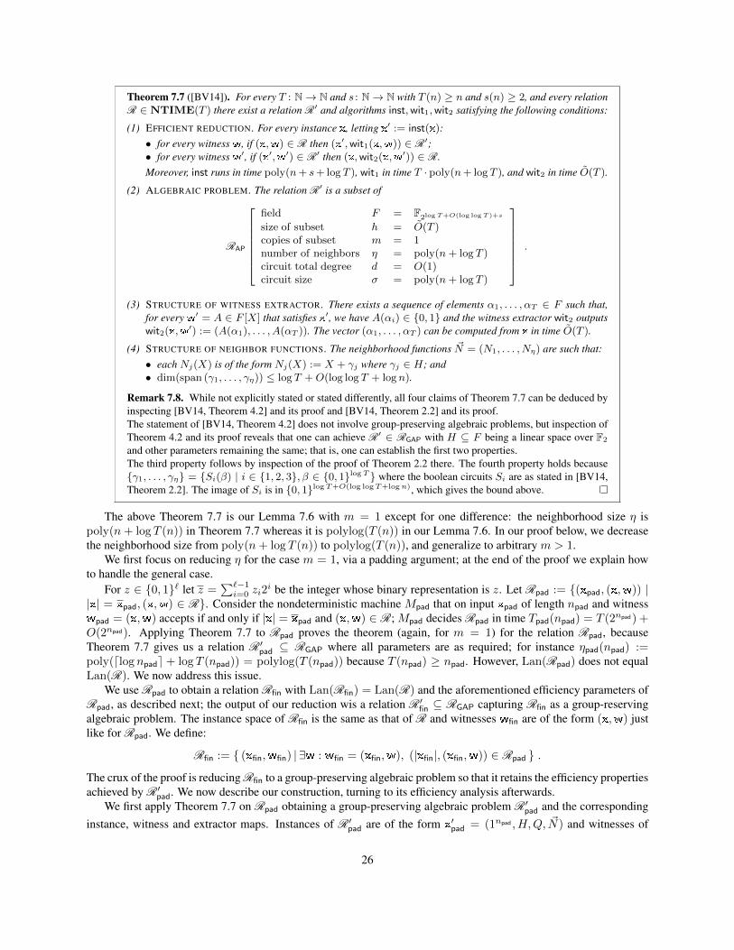
Theorem 7.7 ([BV14]). For every T : N→ N and s : N→ N with T (n) ≥ n and s(n) ≥ 2, and every relationR ∈ NTIME(T ) there exist a relation R′ and algorithms inst,wit1,wit2 satisfying the following conditions:

(1) EFFICIENT REDUCTION. For every instance x, letting x′ := inst(x):• for every witness w, if (x,w) ∈ R then (x′,wit1(x,w)) ∈ R′;• for every witness w′, if (x′,w′) ∈ R′ then (x,wit2(x,w′)) ∈ R.Moreover, inst runs in time poly(n+ s+ log T ), wit1 in time T · poly(n+ log T ), and wit2 in time O(T ).

(2) ALGEBRAIC PROBLEM. The relation R′ is a subset of

RAP


size of subset h = O(T )copies of subset m = 1number of neighbors η = poly(n+ log T )circuit total degree d = O(1)circuit size σ = poly(n+ log T )

.

(3) STRUCTURE OF WITNESS EXTRACTOR. There exists a sequence of elements α1, . . . , αT ∈ F such that,for every w′ = A ∈ F [X] that satisfies x′, we have A(αi) ∈ 0, 1 and the witness extractor wit2 outputswit2(x,w′) := (A(α1), . . . , A(αT )). The vector (α1, . . . , αT ) can be computed from x in time O(T ).

(4) STRUCTURE OF NEIGHBOR FUNCTIONS. The neighborhood functions ~N = (N1, . . . , Nη) are such that:• each Nj(X) is of the form Nj(X) := X + γj where γj ∈ H; and• dim(span (γ1, . . . , γη)) ≤ log T +O(log log T + logn).

Remark 7.8. While not explicitly stated or stated differently, all four claims of Theorem 7.7 can be deduced byinspecting [BV14, Theorem 4.2] and its proof and [BV14, Theorem 2.2] and its proof.The statement of [BV14, Theorem 4.2] does not involve group-preserving algebraic problems, but inspection ofTheorem 4.2 and its proof reveals that one can achieve R′ ∈ RGAP with H ⊆ F being a linear space over F2

and other parameters remaining the same; that is, one can establish the first two properties.The third property follows by inspection of the proof of Theorem 2.2 there. The fourth property holds becauseγ1, . . . , γη = Si(β) | i ∈ 1, 2, 3, β ∈ 0, 1log T where the boolean circuits Si are as stated in [BV14,Theorem 2.2]. The image of Si is in 0, 1log T+O(log log T+logn), which gives the bound above.

The above Theorem 7.7 is our Lemma 7.6 with m = 1 except for one difference: the neighborhood size η ispoly(n+ log T (n)) in Theorem 7.7 whereas it is polylog(T (n)) in our Lemma 7.6. In our proof below, we decreasethe neighborhood size from poly(n+ log T (n)) to polylog(T (n)), and generalize to arbitrary m > 1.

We first focus on reducing η for the case m = 1, via a padding argument; at the end of the proof we explain howto handle the general case.

For z ∈ 0, 1` let z =∑`−1i=0 zi2

i be the integer whose binary representation is z. Let Rpad := (xpad, (x,w)) ||x| = xpad, (x,w) ∈ R. Consider the nondeterministic machine Mpad that on input xpad of length npad and witnesswpad = (x,w) accepts if and only if |x| = xpad and (x,w) ∈ R; Mpad decides Rpad in time Tpad(npad) = T (2npad) +O(2npad). Applying Theorem 7.7 to Rpad proves the theorem (again, for m = 1) for the relation Rpad, becauseTheorem 7.7 gives us a relation R′pad ⊆ RGAP where all parameters are as required; for instance ηpad(npad) :=poly(dlog npade + log T (npad)) = polylog(T (npad)) because T (npad) ≥ npad. However, Lan(Rpad) does not equalLan(R). We now address this issue.

We use Rpad to obtain a relation Rfin with Lan(Rfin) = Lan(R) and the aforementioned efficiency parameters ofRpad, as described next; the output of our reduction wis a relation R′fin ⊆ RGAP capturing Rfin as a group-reservingalgebraic problem. The instance space of Rfin is the same as that of R and witnesses wfin are of the form (x,w) justlike for Rpad. We define:

Rfin := (xfin,wfin) | ∃w : wfin = (xfin,w), (|xfin|, (xfin,w)) ∈ Rpad .

The crux of the proof is reducing Rfin to a group-preserving algebraic problem so that it retains the efficiency propertiesachieved by R′pad. We now describe our construction, turning to its efficiency analysis afterwards.

We first apply Theorem 7.7 on Rpad obtaining a group-preserving algebraic problem R′pad and the correspondinginstance, witness and extractor maps. Instances of R′pad are of the form x

′pad = (1npad , H,Q, ~N) and witnesses of

26

R′pad are of the form w′pad = (A), where A is an assignment polynomial. Property (3) of Theorem 7.7 implies that

for every A that satisfies x′pad := inst(x), the sequence wpad := (A(α1), . . . , A(αn+T )) belongs to 0, 1n+T and(xpad,wpad) ∈ Rpad. It follows that the sequence x′ := (A(α1), . . . , A(αn)) belongs to Lan(R). However, asexplained above Lan(R) 6= Lan(Rpad): while |x| = |x′|, the x′ does not necessarily equal x. We now explain how tomodoify Rpad so it encodes a concrete instance x, not just fixes its length |x|.

We define an auxiliary instance xaux of RGAP to be xaux := (1npad , Haux, Qaux, ~Naux), where we chooseHaux,Qaux,~Naux as follows:• Haux := β +H , where β ∈ F \H (so Haux is a β-coset of H);• ηaux := 1 and Naux,1(X) := X − β; and• Qaux(X,Y1) :=

∑ni=1 Zβ+(H\αi)(X) · (Y1 − xi).

It can be verified that A satisfies xaux if and only if x′ defined above equals x: indeed, when evaluating (Qaux A ~Naux)(αi) all terms vanish except for Zβ+(H\αi)(αi) · (xi− x′i). We now use the fact that if set S consists of allpoints of an affine subspace, then the polynomial ZS(X) has at most dim(S) + 1 non-zero terms [Ore33]. Therefore,each summand of Qaux can be computed by an arithmetic circuit of size O(dim(H)2) because each β + (H \ αi)can be partitioned in dim(H) affine subspaces as β + (H \ αi) =

⋃dim(H)−1i=0 (βi +Hi), where the affine subspace

βi +Hi has dimension i.1

We combine xaux and x′pad to obtain x′fin := (1npad , Hfin, Qfin, ~Nfin) as follows:• Hfin := H ∪ (β +H);• ηfin := η + 1 and ~Nfin := ~N ∪ ~Naux = ~N1, . . . , ~Nη, ~Nη+1 := (X − β); and• Qfin(X,Y1, . . . , Yη+1) := Zβ+H(X) ·Q(X,Y1, . . . , Yη) + ZH(X) ·Qaux(X,Yη+1).It can also be verified that A satisfies xaux if and only if A encodes instance x′ and witness w′ with (x′,w′) ∈ R andx = x

′. We now verify that all parameters of R′fin match those in the statement of Lemma 7.6.All parameters are closely tied to those of R′pad and are established as follows. F is inherited from R′pad and is

F2log T+O(log log T )+s . The vanishing set has size hfin = O(T ), which matches the theorem statement asm = 1. Numberof neighborhood functions is polylog(T ) and total degree of Y in Qfin is d = O(1), both as required. Since β +H isan affine space and H is a linear space we see that Qfin can be computed by a circuit of size σfin = σpad + polylog(T )because dim(H) = O(log T (n)) (again, using the theorem of [Ore33]). Finally, Hfin is an additive group (it is unionof a linear space space and its shift and char(F ) = 2) and it can be verified that each ~Nfin,j satisfies ~Nfin,j(H) ⊆ H∗,therefore x′fin ∈ R′pad as claimed.

We now prove the case m = m(n) > 1. First, we invoke the reduction described above on R, next we modifyits output R′fin to achieve the required parameters m and h, as follows. Suppose that R′fin is defined over field Ffin

with |Ffin| = 2r and the vanishing set Hfin has size hfin. The theorem statement guarantees that hm = Ω(T log T )and therefore r ≤ h ·m. We first discuss the case that r = h ·m. Notice that the additive group F+

2r is isomorphicto (F+

2h)m, therefore H+

fin ⊆ F+2r is isomorphic to some Hm and we are done. If r < h ·m, then we just increase the

dimension of the field Ffin and modify Qfin to vanish whenever any variable Xi is set in the padded coordinates. Noother parameters are changed, except for the gain of an additive m term in σ to account for the additional constraints.

7.5 Combining the two reductionsBy combining Lemma 7.6 and Lemma 7.5, we obtain the following theorem, which gives the reduction claimed at thebeginning of this section.

Theorem 7.9 (NTIME → RRLA). For every T, t, s : N → N, δ, ε : N → (0, 1) with 2s(n) ≥ Ω( t(1−δ)Tpolylog(T ) ),

and R ∈ NTIME(T ) there exist a relation R′ and algorithms inst,wit1,wit2 satisfying the following conditions:


– for every witness w, if (x,w) ∈ R then (x′,wit1(x,w)) ∈ R′;

1For example, one can express αi in the basis of H and define βi +Hdim(H)−k to be the affine subspace where first k − 1 basis vectors arefixed with coefficients equal to that of αi, k-th basis vector is fixed with the opposite coefficient, and the last dim(H) − k basis vectors remainunfixed.

27

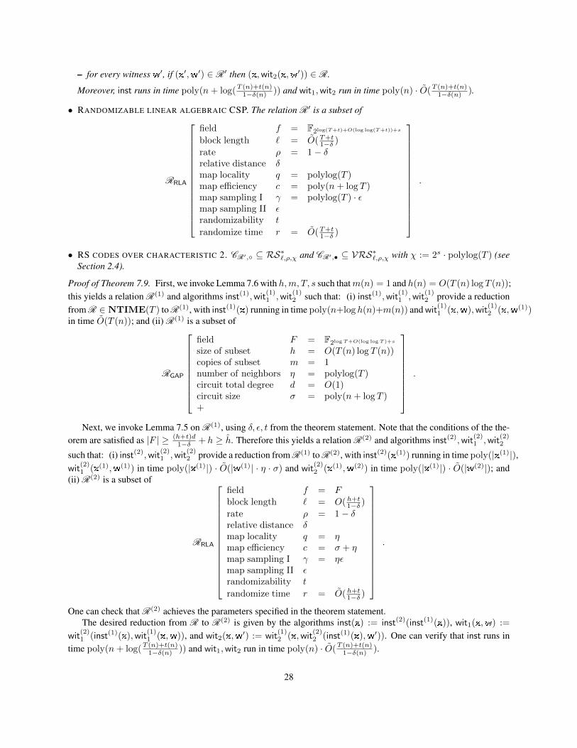
– for every witness w′, if (x′,w′) ∈ R′ then (x,wit2(x,w′)) ∈ R.

Moreover, inst runs in time poly(n+ log(T (n)+t(n)1−δ(n) )) and wit1,wit2 run in time poly(n) · O(T (n)+t(n)

1−δ(n) ).

• RANDOMIZABLE LINEAR ALGEBRAIC CSP. The relation R′ is a subset of

RRLA

field f = F2log(T+t)+O(log log(T+t))+s

block length ` = O(T+t1−δ )

rate ρ = 1− δrelative distance δmap locality q = polylog(T )map efficiency c = poly(n+ log T )map sampling I γ = polylog(T ) · εmap sampling II εrandomizability t

randomize time r = O(T+t1−δ )

.

• RS CODES OVER CHARACTERISTIC 2. CR′, ⊆ RS∗`,ρ,χ and CR′,• ⊆ VRS∗`,ρ,χ with χ := 2s · polylog(T ) (seeSection 2.4).

Proof of Theorem 7.9. First, we invoke Lemma 7.6 with h,m, T, s such thatm(n) = 1 and h(n) = O(T (n) log T (n));this yields a relation R(1) and algorithms inst(1),wit

(1)1 ,wit

(1)2 such that: (i) inst(1),wit

(1)1 ,wit

(1)2 provide a reduction

from R ∈ NTIME(T ) to R(1), with inst(1)(x) running in time poly(n+log h(n)+m(n)) and wit(1)1 (x,w),wit

(1)2 (x,w(1))

in time O(T (n)); and (ii) R(1) is a subset of

RGAP


size of subset h = O(T (n) log T (n))copies of subset m = 1number of neighbors η = polylog(T )circuit total degree d = O(1)circuit size σ = poly(n+ log T )+

.

Next, we invoke Lemma 7.5 on R(1), using δ, ε, t from the theorem statement. Note that the conditions of the the-orem are satisfied as |F | ≥ (h+t)d

1−δ + h ≥ h. Therefore this yields a relation R(2) and algorithms inst(2),wit(2)1 ,wit

(2)2

such that: (i) inst(2),wit(2)1 ,wit

(2)2 provide a reduction from R(1) to R(2), with inst(2)(x(1)) running in time poly(|x(1)|),

wit(2)1 (x(1),w(1)) in time poly(|x(1)|) · O(|w(1)| · η · σ) and wit

(2)2 (x(1),w(2)) in time poly(|x(1)|) · O(|w(2)|); and

(ii) R(2) is a subset of

RRLA

field f = Fblock length ` = O(h+t

1−δ )

rate ρ = 1− δrelative distance δmap locality q = ηmap efficiency c = σ + ηmap sampling I γ = ηεmap sampling II εrandomizability t

randomize time r = O(h+t1−δ )

.

One can check that R(2) achieves the parameters specified in the theorem statement.The desired reduction from R to R(2) is given by the algorithms inst(x) := inst(2)(inst(1)(x)), wit1(x,w) :=

wit(2)1 (inst(1)(x),wit

(1)1 (x,w)), and wit2(x,w′) := wit

(1)2 (x,wit

(2)2 (inst(1)(x),w′)). One can verify that inst runs in

time poly(n+ log(T (n)+t(n)1−δ(n) )) and wit1,wit2 run in time poly(n) · O(T (n)+t(n)

1−δ(n) ).

28

Finally, Lemma 7.6 implies that x(1) = (1n, H,Q, ~N) where H is an additive subgroup of F (n), which hascharacteristic 2. Hence, Lemma 7.5 implies that x(2) = (1n, C, C•, g) where C = RS[F (n), H, h(n)+t(n)

h(n)] ⊆

RS[F (n), H, δ] and C• = VRS[F (n), H, (h(n)+t(n))d(n)

h(n), H] ⊆ VRS[F (n), H, δ,H] where H is a union of cosets of

the subgroup H with cardinality h(n). Thus, C ∈ RS∗`,ρ,χ and C• ∈ VRS∗`,ρ,χ, as claimed.

29

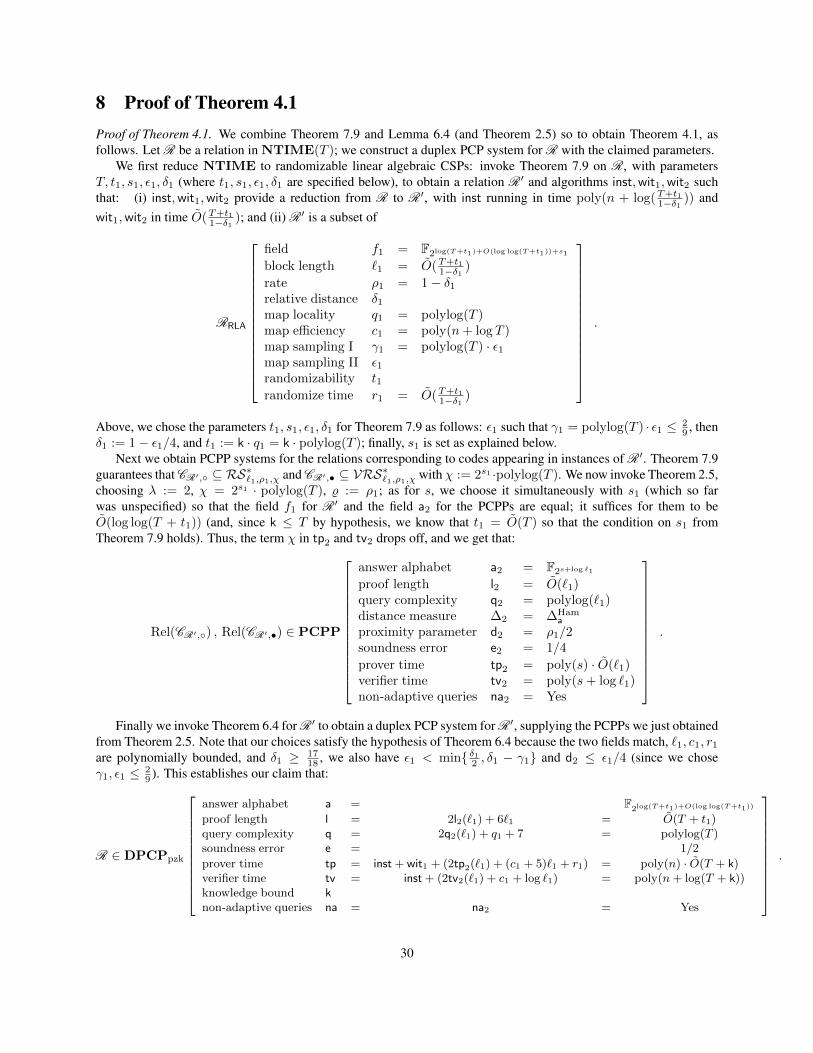
8 Proof of Theorem 4.1Proof of Theorem 4.1. We combine Theorem 7.9 and Lemma 6.4 (and Theorem 2.5) so to obtain Theorem 4.1, asfollows. Let R be a relation in NTIME(T ); we construct a duplex PCP system for R with the claimed parameters.

We first reduce NTIME to randomizable linear algebraic CSPs: invoke Theorem 7.9 on R, with parametersT, t1, s1, ε1, δ1 (where t1, s1, ε1, δ1 are specified below), to obtain a relation R′ and algorithms inst,wit1,wit2 suchthat: (i) inst,wit1,wit2 provide a reduction from R to R′, with inst running in time poly(n + log(T+t1

1−δ1 )) andwit1,wit2 in time O(T+t1

1−δ1 ); and (ii) R′ is a subset of

RRLA

field f1 = F2log(T+t1)+O(log log(T+t1))+s1

block length `1 = O(T+t11−δ1 )

rate ρ1 = 1− δ1relative distance δ1map locality q1 = polylog(T )map efficiency c1 = poly(n+ log T )map sampling I γ1 = polylog(T ) · ε1map sampling II ε1randomizability t1randomize time r1 = O(T+t1

1−δ1 )

.

Above, we chose the parameters t1, s1, ε1, δ1 for Theorem 7.9 as follows: ε1 such that γ1 = polylog(T ) · ε1 ≤ 29 , then

δ1 := 1− ε1/4, and t1 := k · q1 = k · polylog(T ); finally, s1 is set as explained below.Next we obtain PCPP systems for the relations corresponding to codes appearing in instances of R′. Theorem 7.9

guarantees that CR′, ⊆ RS∗`1,ρ1,χ and CR′,• ⊆ VRS∗`1,ρ1,χ with χ := 2s1 ·polylog(T ). We now invoke Theorem 2.5,choosing λ := 2, χ = 2s1 · polylog(T ), % := ρ1; as for s, we choose it simultaneously with s1 (which so farwas unspecified) so that the field f1 for R′ and the field a2 for the PCPPs are equal; it suffices for them to beO(log log(T + t1)) (and, since k ≤ T by hypothesis, we know that t1 = O(T ) so that the condition on s1 fromTheorem 7.9 holds). Thus, the term χ in tp2 and tv2 drops off, and we get that:

Rel(CR′,) , Rel(CR′,•) ∈ PCPP

answer alphabet a2 = F2s+log `1

proof length l2 = O(`1)query complexity q2 = polylog(`1)distance measure ∆2 = ∆Ham

a

proximity parameter d2 = ρ1/2soundness error e2 = 1/4

prover time tp2 = poly(s) · O(`1)verifier time tv2 = poly(s+ log `1)non-adaptive queries na2 = Yes

.

Finally we invoke Theorem 6.4 for R′ to obtain a duplex PCP system for R′, supplying the PCPPs we just obtainedfrom Theorem 2.5. Note that our choices satisfy the hypothesis of Theorem 6.4 because the two fields match, `1, c1, r1

are polynomially bounded, and δ1 ≥ 1718 , we also have ε1 < min δ12 , δ1 − γ1 and d2 ≤ ε1/4 (since we chose

γ1, ε1 ≤ 29 ). This establishes our claim that:

R ∈ DPCPpzk

answer alphabet a = F2log(T+t1)+O(log log(T+t1))

proof length l = 2l2(`1) + 6`1 = O(T + t1)query complexity q = 2q2(`1) + q1 + 7 = polylog(T )soundness error e = 1/2

prover time tp = inst + wit1 + (2tp2(`1) + (c1 + 5)`1 + r1) = poly(n) · O(T + k)verifier time tv = inst + (2tv2(`1) + c1 + log `1) = poly(n+ log(T + k))knowledge bound knon-adaptive queries na = na2 = Yes

.

30

The precise expression for soundness error is e := max1− δ1 + γ1 + ε1 , (1− |f1|−1) ·maxe2, ε1/4+ |f1|−1,but it is upper bounded by 1

2 , because for us 1− δ1 + γ1 + ε1 ≤ 12 , maxe2, ε1/4 = 1

4 and |f1| ≥ 4.

31

AcknowledgmentsWe thank Yuval Ishai and Mor Weiss for helpful discussions. The research leading to these results has received fundingfrom: the European Community’s Seventh Framework Programme (FP7/2007-2013) under grant agreement number240258; the Israeli Science Foundation (grant 1501/14); and the Center for Science of Information (CSoI), an NSFScience and Technology Center, under grant agreement CCF-0939370.

32

References[ALM+98] Sanjeev Arora, Carsten Lund, Rajeev Motwani, Madhu Sudan, and Mario Szegedy. Proof verification and the

hardness of approximation problems. Journal of the ACM, 45(3):501–555, 1998. Preliminary version in FOCS ’92.

[Alo99] Noga Alon. Combinatorial Nullstellensatz. Combinatorics, Probability and Computing, 8(1-2):7–29, Jan 1999.

[AS98] Sanjeev Arora and Shmuel Safra. Probabilistic checking of proofs: a new characterization of NP. Journal of theACM, 45(1):70–122, 1998. Preliminary version in FOCS ’92.

[BCG+16] Eli Ben-Sasson, Alessandro Chiesa, Ariel Gabizon, Michael Riabzev, and Nicholas Spooner. Short interactive oracleproofs with constant query complexity, via composition and sumcheck, 2016. Crypto ePrint 2016/324.

[BCGT13a] Eli Ben-Sasson, Alessandro Chiesa, Daniel Genkin, and Eran Tromer. Fast reductions from RAMs to delegatablesuccinct constraint satisfaction problems. In Proceedings of the 4th Innovations in Theoretical Computer ScienceConference, ITCS ’13, 2013.

[BCGT13b] Eli Ben-Sasson, Alessandro Chiesa, Daniel Genkin, and Eran Tromer. On the concrete efficiency of probabilistically-checkable proofs. In Proceedings of the 45th ACM Symposium on the Theory of Computing, STOC ’13, 2013.

[BCI+13] Nir Bitansky, Alessandro Chiesa, Yuval Ishai, Rafail Ostrovsky, and Omer Paneth. Succinct non-interactive argu-ments via linear interactive proofs. In Proceedings of the 10th Theory of Cryptography Conference, TCC ’13, pages315–333, 2013.

[BCS16] Eli Ben-Sasson, Alessandro Chiesa, and Nicholas Spooner. Interactive oracle proofs, 2016. Crypto ePrint 2016/116.

[BFL91] Laszlo Babai, Lance Fortnow, and Carsten Lund. Non-deterministic exponential time has two-prover interactiveprotocols. Computational Complexity, 1:3–40, 1991.

[BFLS91] Laszlo Babai, Lance Fortnow, Leonid A. Levin, and Mario Szegedy. Checking computations in polylogarithmictime. In Proceedings of the 23rd Annual ACM Symposium on Theory of Computing, STOC ’91, pages 21–32, 1991.

[BG93] Mihir Bellare and Oded Goldreich. On defining proofs of knowledge. In Proceedings of the 12th Annual Interna-tional Cryptology Conference on Advances in Cryptology, CRYPTO ’92, pages 390–420, 1993.

[BGG+88] Michael Ben-Or, Oded Goldreich, Shafi Goldwasser, Johan Hastad, Joe Kilian, Silvio Micali, and Phillip Rogaway.Everything provable is provable in zero-knowledge. In Proceedings of the 8th Annual International CryptologyConference, CRYPTO ’88, pages 37–56, 1988.

[BGH+04] Eli Ben-Sasson, Oded Goldreich, Prahladh Harsha, Madhu Sudan, and Salil Vadhan. Robust PCPs of proximity,shorter PCPs and applications to coding. In Proceedings of the 26th Annual ACM Symposium on Theory of Comput-ing, STOC ’04, pages 1–10, 2004.

[BGH+05] Eli Ben-Sasson, Oded Goldreich, Prahladh Harsha, Madhu Sudan, and Salil Vadhan. Short PCPs verifiable inpolylogarithmic time. In Proceedings of the 20th Annual IEEE Conference on Computational Complexity, CCC ’05,pages 120–134, 2005.

[BGH+06] Eli Ben-Sasson, Oded Goldreich, Prahladh Harsha, Madhu Sudan, and Salil Vadhan. Robust PCPs of proximity,shorter PCPs, and applications to coding. SIAM Journal on Computing, 36(4):889–974, 2006. Preliminary versionsof this paper have appeared in Proceedings of the 36th ACM Symposium on Theory of Computing and in ElectronicColloquium on Computational Complexity.

[BKK+13] Eli Ben-Sasson, Yohay Kaplan, Swastik Kopparty, Or Meir, and Henning Stichtenoth. Constant rate PCPs forCircuit-SAT with sublinear query complexity. In Proceedings of the 54th Annual IEEE Symposium on Foundationsof Computer Science, FOCS ’13, pages 320–329, 2013.

[BM88] Laszlo Babai and Shlomo Moran. Arthur-Merlin games: a randomized proof system, and a hierarchy of complexityclass. Journal of Computer and System Sciences, 36(2):254–276, 1988.

[BOGKW88] Michael Ben-Or, Shafi Goldwasser, Joe Kilian, and Avi Wigderson. Multi-prover interactive proofs: how to removeintractability assumptions. In Proceedings of the 20th Annual ACM Symposium on Theory of Computing, STOC ’88,pages 113–131, 1988.

[BS08] Eli Ben-Sasson and Madhu Sudan. Short PCPs with polylog query complexity. SIAM Journal on Computing,38(2):551–607, 2008. Preliminary version appeared in STOC ’05.

[BV14] Eli Ben-Sasson and Emanuele Viola. Short PCPs with projection queries. In Proceedings of the 41st InternationalColloquium on Automata, Languages and Programming, ICALP ’14, pages 163–173, 2014.

33

[DFK+92] Cynthia Dwork, Uriel Feige, Joe Kilian, Moni Naor, and Shmuel Safra. Low communication 2-prover zero-knowledge proofs for NP. In Proceedings of the 12th Annual International Cryptology Conference, CRYPTO ’92,pages 215–227, 1992.

[Din07] Irit Dinur. The PCP theorem by gap amplification. Journal of the ACM, 54(3):12, 2007.

[DR04] Irit Dinur and Omer Reingold. Assignment testers: Towards a combinatorial proof of the PCP theorem. In Pro-ceedings of the 45th Annual IEEE Symposium on Foundations of Computer Science, FOCS ’04, pages 155–164,2004.

[GIMS10] Vipul Goyal, Yuval Ishai, Mohammad Mahmoody, and Amit Sahai. Interactive locking, zero-knowledge PCPs, andunconditional cryptography. In Proceedings of the 30th Annual International Cryptology Conference, CRYPTO ’10,pages 173–190, 2010.

[GMR85] Shafi Goldwasser, Silvio Micali, and Charles Rackoff. The knowledge complexity of interactive proof-systems. InProceedings of the 17th Annual ACM Symposium on Theory of Computing, STOC ’85, pages 291–304, 1985.

[HS00] Prahladh Harsha and Madhu Sudan. Small PCPs with low query complexity. Computational Complexity, 9(3–4):157–201, Dec 2000. Preliminary version in STACS ’91.

[IKOS09] Yuval Ishai, Eyal Kushilevitz, Rafail Ostrovsky, and Amit Sahai. Zero-knowledge proofs from secure multipartycomputation. SIAM J. Comput., 39(3):1121–1152, 2009.

[IMS12] Yuval Ishai, Mohammad Mahmoody, and Amit Sahai. On efficient zero-knowledge PCPs. In Proceedings of the 9thTheory of Cryptography Conference on Theory of Cryptography, TCC ’12, pages 151–168, 2012.

[IMSX15] Yuval Ishai, Mohammad Mahmoody, Amit Sahai, and David Xiao. On zero-knowledge PCPs: Limitations, sim-plifications, and applications, 2015. Available at http://www.cs.virginia.edu/˜mohammad/files/papers/ZKPCPs-Full.pdf.

[IW14] Yuval Ishai and Mor Weiss. Probabilistically checkable proofs of proximity with zero-knowledge. In Proceedingsof the 11th Theory of Cryptography Conference, TCC ’14, pages 121–145, 2014.

[IWY16] Yuval Ishai, Mor Weiss, and Guang Yang. Making the best of a leaky situation: Zero-knowledge PCPs from leakage-resilient circuits. In Proceedings of the 13th Theory of Cryptography Conference, TCC ’16, pages 3–32, 2016.

[IY87] Russell Impagliazzo and Moti Yung. Direct minimum-knowledge computations. In Proceedings of the 7th AnnualInternational Cryptology Conference, CRYPTO ’87, pages 40–51, 1987.

[KPT97] Joe Kilian, Erez Petrank, and Gabor Tardos. Probabilistically checkable proofs with zero knowledge. In Proceedingsof the 29th Annual ACM Symposium on Theory of Computing, STOC ’97, pages 496–505, 1997.

[KR08] Yael Tauman Kalai and Ran Raz. Interactive PCP. In Proceedings of the 35th International Colloquium on Automata,Languages and Programming, ICALP ’08, pages 536–547, 2008.

[LFKN92] Carsten Lund, Lance Fortnow, Howard Karloff, and Nisan Noam. Algebraic methods for interactive proof systems.Journal of the ACM, 39(4):859–868, 1992.

[LS95] Dror Lapidot and Adi Shamir. A one-round, two-prover, zero-knowledge protocol for NP. Combinatorica,15(2):204–214, 1995.

[Mie08] Thilo Mie. Polylogarithmic two-round argument systems. Journal of Mathematical Cryptology, 2(4):343–363,2008.

[MX13] Mohammad Mahmoody and David Xiao. Languages with efficient zero-knowledge pcps are in SZK. In Proceedingsof the 10th Theory of Cryptography Conference, TCC ’13, pages 297–314, 2013.

[Ore33] Oystein Ore. On a special class of polynomials. Transactions of the American Mathematical Society, 35(3):559–584,1933.

[OW93] Rafail Ostrovsky and Avi Wigderson. One-way functions are essential for non-trivial zero-knowledge. In Proceed-ings of the 2nd Israel Symposium on Theory of Computing Systems, ISTCS ’93, pages 3–17, 1993.

[PS94] Alexander Polishchuk and Daniel A. Spielman. Nearly-linear size holographic proofs. In Proceedings of the 26thAnnual ACM Symposium on Theory of Computing, STOC ’94, pages 194–203, 1994.

[RRR16] Omer Reingold, Ron Rothblum, and Guy Rothblum. Constant-round interactive proofs for delegating computation.In Proceedings of the 48th ACM Symposium on the Theory of Computing, STOC ’16, pages ???–???, 2016.

[Sha92] Adi Shamir. IP = PSPACE. Journal of the ACM, 39(4):869–877, 1992.

34

http://www.cs.virginia.edu/~mohammad/files/papers/ZKPCPs-Full.pdf

http://www.cs.virginia.edu/~mohammad/files/papers/ZKPCPs-Full.pdf

[Spi95] Daniel Spielman. Computationally Efficient Error-Correcting Codes and Holographic Proofs. PhD thesis, Mas-sachusetts Institute of Technology, 1995.

[Sze99] Mario Szegedy. Many-valued logics and holographic proofs. In Proceedings of the 26th International Colloquiumon Automata, Languages and Programming, ICALP ’99, pages 676–686, 1999.

35

Quasilinear-Size Zero Knowledge from Linear … Zero Knowledge from Linear-Algebraic PCPs Eli...

Documents

Transcript of Quasilinear-Size Zero Knowledge from Linear … Zero Knowledge from Linear-Algebraic PCPs Eli...