Quasars in the SDSSclassic.sdss.org/education/kron_quasars.pdf · parameters of quasars in the SDSS...
51
NGC 1068 Quasars in the SDSS Rich Kron 28 June 2006 START CI-Team: Variable Quasars Research Workshop Yerkes Observatory
Transcript of Quasars in the SDSSclassic.sdss.org/education/kron_quasars.pdf · parameters of quasars in the SDSS...

NGC 1068
Quasars in the SDSSRich Kron
28 June 2006START CI-Team: Variable Quasars Research Workshop
Yerkes Observatory

About 10% of all of the spectra in the SDSS database are of quasars (as opposed to galaxies and stars).
We selected quasars deliberately because they are extremely luminous: we can see them to huge distances, which allows us to map an enormous volume of space.
A census of the quasars shows that they were more common and/or more luminous billions of years ago.

Statistical studies are greatly helped by the SDSS design: uniform selection, uniform data quality, and good calibrations.
And, of course, large numbers: 80,000 quasar spectra in DR5, expect more than 100,000 at the end of operations.

In order to get a spectrum, we need first to identify an object as a possible quasar, based on the u g r i z imaging data of the SDSS.
This is done by exploiting the property that quasars do not shine by the same processes that stars do.
That means that their colors (u-g, g-r, r-i, i-z) will be unlike the colors of normal stars.

19.5 < g < 20.5
-0.5
0
0.5
1
1.5
2
-0.5 0 0.5 1 1.5 2 2.5 3 3.5
u-g
g-r
region of sky:200 < ra < 202.543 < dec < 45.5


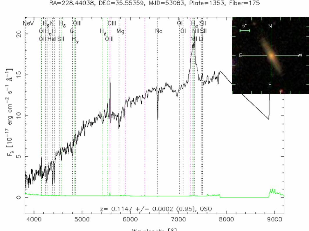
After spectra are obtained of all of the candidate quasars, how is it determined which ones really are quasars?
An automated analysis “pipeline” is run on each spectrum.
The algorithm looks for the presence of broad emission lines, which are characteristic of quasars.

Sun-like star

hot star

H II region

⇒ light is non-stellar⇒ emission lines are broad

More quantitatively:
The software detects absorption and emission lines, and fits a Gaussian function to each line profile.
The parameters are:
height (10-17 erg sec-1 cm-2 Å-1); + = em, - = abscontinuum (10-17 erg sec-1 cm-2 Å-1)sigma (Ångstroms)

SDSS adopts a practical definition of a quasar: at least one line must have a full-width at half-maximum (FWHM) broader than 1000 km/sec.
to convert from sigma in Ångstroms to FWHM in km/sec:
FWHM = c × [(2.354 × sigma) / λ]
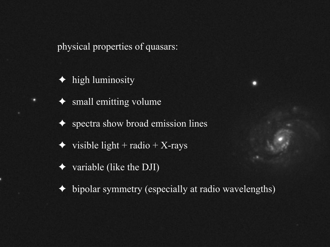
physical properties of quasars:
high luminosity
small emitting volume
spectra show broad emission lines
visible light + radio + X-rays
variable (like the DJI)
bipolar symmetry (especially at radio wavelengths)

physical model:
central supermassive black hole that is accreting gas
gas falls into the black hole because of viscosity (drag)
as the gas falls, the gravitational energy of falling is converted into heat and light

the emitting region (active nucleus) is tiny:
Mbh = 3 × 10⁷ Msun
RSch = 2 G Mbh / c2 = 0.6 AU
Raccretion ~ 10 RSch = 6 AU = 50 light-minutes
compare to:diameter of a galaxy ~ 70,000 light-years
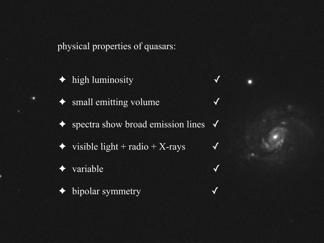
physical properties of quasars:
high luminosity ✓small emitting volume ✓spectra show broad emission lines ✓visible light + radio + X-rays ✓variable ✓bipolar symmetry ✓

parameters of quasars in the SDSS database:
redshift ≡ distance
apparent brightness in different filters; colors
image structure
linesheightsigmacontinuum

converting redshift to distance for quasars:
the symbol for the measured quantity of redshift is z
naive relation:
d = (c/H0) × z = 4200 megaparsecs × z
= 13.7 billion light-years × z
this is OK as long as z << 1

converting redshift to distance for quasars, continued:
since the distances are so large, effects such as the geometrical curvature of space (non-Euclidean geometry) are important
moreover, in an expanding Universe, the distances between all objects are increasing with time
⇒ what exactly is meant by “distance?”

what exactly is meant by “distance?”
L = 4π d2 × b d is “luminosity distance”
R = d × θ d is “angular-size distance”
You can get the values for these distances at
http://www.astro.ucla.edu/~wright/CosmoCalc.html
1) enter the redshift into the “z” window2) leave the default cosmological parameters as they are3) press “flat”

how do I get quasar data out of the SDSS database?
go to sdss.org ,
click on “skyserver,” then “search,” then “SQL”


the shape of a quasar emission line on a plot of flux versus wavelength is called the profile
if all the emitting gas were quiescent (no relative motion), then the line would look like a narrow spike
⇒ analysis of the profile tells us about the velocity distribution of the emitting gas

The velocity distribution of the emitting gas could be due to pressure of some sort (like weather, winds). For example, gas in the Milky Way is pushed around by the expanding shells of supernovae.
If there is no pressure, gas in a circular orbit around a mass M at radius R would have a velocity
v2 = G M / R
where G is Newton’s gravitational constant
v for Earth orbiting the Sun = 30 km/sec
v for Sun orbiting the center of the Milky Way = 220 km/sec

The Doppler shift allows us to determine the velocity from a measurement of the observed wavelength.
The Doppler shift only measures the part of the velocity that is along the line-of-sight.
By convention, positive means motion away from us, negative means motion towards us.

how fast is the gas moving inside this quasar?
Δλ = 600 Å, λ = 7600 Å v / c = Δλ / λ = 0.08v = 24,000 km/sec (!)
Δλ
v / c = Δλ / λ

If we can find the quasars with the widest lines, we would find the ones with gas moving at the highest velocities.
This is interesting because we would then be looking relatively close to the central black hole: high v means a high value for the quantity M/R (if the motion is due to gravity).
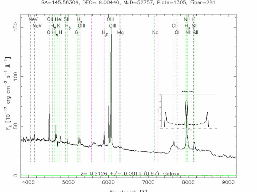
What do we know about quasars with the widest lines?

Chen, Halpern, and Filippenko 1989
double-peaked line profile for Arp 102B: evidence for an accretion disk?

SELECT S.z, S.ra, S.dec, S.plate, S.mjd, S.fiberid,S.mag_0, S.mag_1, S.mag_2, S.zConf, L.continuum, L.height, L.sigma, L.ew
FROM specobj as S, specline as L
WHERE L.specobjid = S.specobjid and(S.z between 0.1 and 0.36) andL.lineID = 6565 and L.category = 2 andL.height > 3 and L.sigma > 50 andS.sn_1 > 15
this query finds broad Hα emission lines:


model line profile
0
50
100
150
200
250
7500 7600 7700 7800 7900 8000 8100 8200 8300 8400 8500
wavelength
inte
nsi
ty
model: transparent, edge-on ring of gas orbiting at 18000 km/sec
model line profile
0
50
100
150
200
250
7500 7600 7700 7800 7900 8000 8100 8200 8300 8400 8500
wavelength
inte
nsi
ty
some ideas for projects:
within the “supernova stripe” area, look for spectroscopic objects with high S/N but low zConf. These could be BL Lac objects. BL Lac objects are highly variable. The supernova database http://www.sdss.org/drsn1/DRSN1_data_release.html enables study of their variability.
correlate a list of hard X-ray sources with the footprint of the supernova stripe (300 < ra < 60; -1.25 < dec < 1.25). Identify optical counterparts and look for variability.
search for changes in line profiles among quasars on the spectroscopic plates observed multiple times. Quasars with wide lines might vary on relatively short time scales. Wilhite did not look at z < 0.5.
for quasars at sufficiently low z that the host galaxy can be seen, investigate whether there are correlations between the properties of the emission lines (e.g. width, shape) and the properties of the host galaxy (e.g. inclination angle, luminosity)

run 2738, November 2001
run 5823, November 2005