QUARTERLY OF APPLIED MATHEMATICS - ams.org€¦arises because of the random motion of electrons in...

129

QUARTERLY OF APPLIED MATHEMATICSVol. VII JULY, 1949 No. 2

THE SPECTRUM OF FREQUENCY-MODULATED WAVESAFTER RECEPTION IN RANDOM NOISE-P

BY

DAVID MIDDLETONCruft Laboratory, Harvard University

Part I: Introduction and Discussion

The reception of radio, radar, and television signals is always accomplished in thepresence of noise, which exclusive of outside sources—either man-made or natural—arises because of the random motion of electrons in the various circuit elements of thereceiver, principally in the stages preceding the detecting devices. The noise is ac-cordingly assumed to be of the fluctuation type; impulse noise is not considered in thispaper. Knowledge of the spectral distribution and the power output following demodu-lation of a frequency-modulated carrier in such noise is essential to any critical theoryof receiver behavior. Accordingly, the principal purpose of the present work is to in-vestigate the spectral aspects of the problem. One of the chief reasons for our interestin the spectrum lies in the fact that the signal-to-noise ratio at the output as a functionof the ratio at the input depends markedly on the spectral distribution, in the so-calledcase of broad-band FM (where the maximum change in carrier frequency may be severaltimes the highest modulating components). The dependence in the instance of narrow-band FM (for which the maximum deviation in the carrier frequency is comparable withor less than the highest significant audio modulating frequency) is not nearly so critical.

Previous investigations, of which the work of Carson and Fry,1 Crosby,2 Blachman,3and Rice4 are particularly to be noted here,** have dealt chiefly with the strong-carriercase, in which the noise is largely suppressed and appears linearly with the signal in

*Received May 27, 1948. The research reported in this document was made possible through supportextended Cruft Laboratory, Harvard University, jointly by the Navy Department (Office of NavalResearch) and the Signal Corps, U. S. Army, under contract N50RI-76, T.O.I. The author wishes tothank Miss Marilyn Lang of the Electronics Research Laboratory, who performed most of the calcula-tions in this paper.

JJ. R. Carson and T. C. Fry, Variable frequency electric circuit theory with application to the theoryof frequency modulation, Bell Syst. Tech. J. 16, 513 (1937).

2M. C. Crosby, Frequency modulation noise characteristics, Proc. I. R. E. 25, 472 (1937).3N. M. Blachman, A theoretical study of the demodulation of a frequency-modulated carrier and random

noise by an FM receiver, Thesis (Harvard, June, 1947). Technical Report No. 31, (1948), Cruft Labora-tory, Harvard University. See also N. M. Blackman, J. Appl. Phys. 20, 38 (1949).

4S. O. Rice, Statistical properties of a sine-wave and random noise, Bell Syst. Tech. J. 27, 109 (1948).**An interesting paper by F. L. H. M. Stumpers (Proc. I.R.E. 36, 1080 (1948) has since appeared,

giving some of the same general conclusions reached here in the case of extreme limiting. The case of nolimiting, however, is not discussed.

130 DAVID MIDDLETON [Vol. VII, No. 2

the output. Rice's work4 is an exception, in that he determines the spectrum for thecase of arbitrary input carrier-to-noise power ratio (p), but only for the idealized ex-ample of extreme limiting (as do likewise Carson and Fry1 and Crosby2). Further, thecarrier is not modulated. Blachman's interesting treatment,3 on the other hand, is morecomprehensive, since he includes modulation and a discussion of the case of no limiting.Similarly, the present paper is more general than Rice's work in that modulation andno limiting are also considered, and is an extension of Blachman's efforts5 since spectra(and their associated correlation functions) are obtained for all values of the ratio p.

We consider the case of no limiting because it gives us one extreme of receiver per-formance as a function of limiting; superlimiting gives us the other. Since the passagefrom the former to the latter is monotonic, we may be able roughly to estimate thebehavior for intermediate degrees of limiting. The ability to handle all values of inputcarrier-to-noise power ratios is particularly useful when we desire the spectrum forthreshold signals (p ^ 1 or less), an important region when contrasting the maximumsensitivities of AM and FM reception. Specific calculations of spectra are made, whichutilize a Gaussian input noise distribution. This spectral shape is usually a somewhatbetter fit to actual responses than the rectangular spectrum. The results of the analysisare given in detail in Part II, while Part III contains a treatment of important specialcases: (1) noise alone, (2) unmodulated carrier and noise, and (3) a sinusoidally modu-lated carrier in noise.

The actual nonlinear or demodulating elements in an FM receiver are too involvedto yield satisfactorily to direct treatment, but a possible model of these essential circuitelements—the limiter, followed by the discriminator—may be constructed if we assumethat the physical discriminator is replaced by an "ideal" one which responds every-where linearly with frequency (the "quasi-stationary" hypothesis of Carson and Fry).Thus, the output current (or voltage) is directly proportional to the instantaneousdifference frequency between the wave and the central or resonant frequency of theIF, limiter, and discriminator bands (all tuned to the same frequency and assumed tobe symmetrical). The filter characteristic of the limiter is taken to be wide enough topass the IF portion of the limited signal and noise without distortion due to frequencyselection. In practice, of course, the real discriminator saturates for sufficiently largeexcursions about resonance, but such behavior is rare if only an insignificant portionof the wave's energy is redistributed into higher harmonics due to the "spreading"action of the limiter.6 This is assumed to be true here even for the extremes of super-limiting, in which the incoming disturbance is heavily clipped at top and bottom.

5Blachman has shown (ref. 3, ch. IV) that when there is no limiting, the characteristic functionmethod used by Rice and others8 in the solution of AM receiver problems may be adapted for all carrierstrengths to the problem in which the idealized discriminator is replaced by one closer to actual electronicpractice, namely, two diode rectifiers ir radians out of phase with one another. Unfortunately, themethod breaks down when there is limiting, since it does not seem practicable to determine, in anyuseful form, the distribution functions Wi and W% of the clipped, filtered noise and signal waves leavingthe limiter to enter a second nonlinear device of the above type. Kac and Siegert (J. Appl. Phys. 18,383 (1947)) have calculated the first-order distribution Wi , but it is the second-order density W-i thatis needed for the spectrum. (The analysis of the present paper has been extended by the author toinclude arbitrary limiting, with the idealized discriminator and similar assumptions as to the widthof the limiter's filter response. See Technical Report No. 62, Cruft Laboratory, Harvard University,Nov. 24, 1948).

6D. Middleton, The response of biased, saturated linear and quadratic rectifiers to random noise,J. Appl. Phys. 17, 778 (1946).

1949] SPECTRUM OF FREQUENCY-MODULATED WAVES 131

The wave leaving the IF and entering the limiter is narrow-band, that is to say, itmay be represented analytically by

V(t) = R(t) cos [oj0£ + 0{t)], (1.1)

where f( = o}0/2ir) is the central frequency of the IF, limiter, and discriminator, R isthe envelope and 8 a phase angle; both R and 6 are slowly varying functions of timecompared with u0t. If we let f(iz) be the Fourier transform of the limiter's dynamiccharacteristic g(V), i.e.

f(iz) = f" e-"vg(V) dV, (1.2)Jo

the output of the limiter may be written7 8

F0(<) = f fdz) exP faR cos (ai0t + 6)] dz. (1.3)Zt J c

The contour C extends along the real axis from — °° to + °° and is indented downwardabout a possible singularity at the origin. With the help of the expansion

exp (ia cos <f>) = ^ intnJn{a) cos n<t>, e0 = 1, e„>, = 2, (1.4)7J = 0

we obtain from (1.3)CO

Vo(t) = S Bn(R) cos n(w0t + d), (1.5)n = 0

where

Bn{R) = ^ Jc f(iz)Jn(Rz) dz. (1.6)

The quantities Bn(R) are the envelopes of the n ( = 0, 1, 2, • • •) spectral zones that areproduced in the limiter by its nonlinear action;7,8 nd is the phase relative to nw0t, then-th harmonic of the original central (angular) frequency. Only the band centeredabout f„(n = 1) is passed to enter the discriminator. The input wave is therefore

V»_d = Bi(R) cos (w0t + 6). (1.7)

In vector language, this input is represented by V,^ = Ve'*, where real quantitiescorrespond to the ^-components, and imaginary quantities to the ^-components. HereV = Bi(R) and $ = u0t + 6. Then we have

Vi-.d = F(cos $ + i sin <£) + F€>(—sin $ + i cos $) = rV + 0F$,

since the polar unit vectors (r, 0) are related to the rectangular ones by the transforma-tion

r = cos $ + i sin <£, 0 = —sin $ + i cos $;

V is the time-rate-of-change of the modulus, and is the time-derivative of the

7S. O. Rice, Mathematical analysis of random noise, Bell Syst. Tech. J. 24, 46 (1945).8D. Middleton, Some general results in the theory of noise through nonlinear devices, Quart. Appl.

Math. 5, 445 (1948). (D. M. I.)

132 DAVID MIDDLETOiN [Vol. VII, No. 2

phase, or, what is the same thing, the instantaneous frequency.9 The output E'0 of ouridealized discriminator is precisely this second term, namely

E'a(t) = kF6 = kB.ORXcoo + 6),

where k is a constant of proportionality with the dimensions (sees). In practice thehigh frequency term, represented above as the coefficient of o>0 , is not passed by thediscriminator filter, so that the final discriminator output is

E?0(<) = KB,{R)e = — [ f(iz)Ji(Rz) dz. (1.9)7T C

Notice that the effect of the limiter is contained in the term B1(R), the exact form ofwhich depends on our choice of g{V), cf. (1.2). We assume that the limiter amplifieslinearly (for both positive and negative amplitudes) up to a certain level, denoted by

Vj_d(tl/2

Fig. 1. A typical limiter characteristic.

R0 , beyond which point saturation occurs abruptly. The dynamic characteristic isshown schematically in Fig. 1. From (1.2) we find that here

f(iz) = 2/3(1 — exp [—iR0z])/{izY, (1.10)

where /3 is the dynamic transfer constant of the limiter and the factor 2 is present be-

9B. van der Pol, The f undamental principles of frequency modulation, Jour. I. E. E. 93, Part III,153 (1946).


cause both the positive and negative portions contribute to the envelope. Accordingly,ft, (ft) in (1.9) is10

ft, (ft) = - [ (i - e~iB")Ji(Rz) -f = 0R, 0 < R < R0 , (1.11a)7r J c z

= - £ft„ 2Fi( —1/2, 1/2; 3/2; ft*/ft2),7T

2 jft„ / ft2\1/2 . /e0-Jr\rV-W) +sm «

fto < ft. (1.11b)

The two cases of chief interest are (a), no limiting, and (b), superlimiting. From (1.11a)and (1.11b) it is evident that ft,(ft) = BR (no limiting); and B, (ft) = (4./ir')ftRn (super-limiting) in which the rms saturation level for the envelope is much less than the inputnoise level (60)1/2, i.e. fto « 2b0 .

Although the spectral behavior of the discriminator output depends on a considerablenumber of parameters, chief among them (1) carrier strength, (2) degree of limiting,(3) power and spectral distribution of the noise entering the demodulating elements, (4)deviation from resonance, (5) intensity and wave-form of the modulation, etc., certaingeneral observations can be made with regard to these factors and their effect on thepower output and spectrum. We summarize the more significant features below, referringto the appropriate figures and equations, the analytical details of whose derivation areavailable in Parts II and III.

1. Signal Output (Power and Spectrum). Spectrally speaking, the modulation isreproduced without distortion (2.32), since our model of the discriminator respondslinearly to all frequencies about resonance. In practice, this is only approximate, be-cause of unavoidable nonlinearities which result in harmonics of the modulation in thelow-frequency output. The effect is small, however, if the maximum deviation remainsmostly in the linear portion of the discriminator characteristic.

Figure 2 illustrates the output signal power fto(0)(sX«> [Eq. (2.32)] as a function ofthe input carrier-to-noise power ratio p. A significant difference between the limitingand non-limiting conditions of receiver operation is immediately evident. For no limiting(X = 1) and sufficiently large values of p (p2 » 1) the output signal power is directlyproportional to p, while for extreme limiting (X = 2) saturation is observed: the outputsignal strength is independent (^p°) of the carrier. The amount of noise is assumed tobe constant in both instances.

On the other hand, the threshold behavior for weak signals (p < 1) shows that thesignal output of the discriminator is proportional to p2, whether or not there is limiting.Thus, if the carrier is sufficiently weak, the limiter-discriminator combination behaveslike any (half-wave) second detector acting on an AM wave,11 as far as the dependenceon carrier strength is concerned. Similar remarks apply for the d-c output (Fig. 2),

10The integration is readily accomplished by representing exp (—iBoz) as the sum of two Besselfunctions and evaluating the resulting Weber-Schafheitlin integrals with the help of Eq. (2), p. 491,Watson, Theory of Bessel functions (Macmillan, 1945). See also D. M. I., Appendix III.

UD. Middleton, Rectification of a sinusoidally modulated carrier in the presence of noise, Proc. I. R. E.,36, 1467 (1948).


provided that we replace the mean-square modulation by the square of the mean.Accordingly, when the modulation possesses no d-c component, there will be no d-coutput, [cf. (2.36), (2.37)]. From these equations and from physical considerations itis also obvious that if the modulation is slow enough, r/ = 0, there will be no observablesignal.

O 1.0 2.0 3.0 P 4.0 5.0

Fig. 2. Output signal power for no limiting (X = 1) and extreme limiting (X = 2).

2. Noise Output (Power). The low-frequency noise power from the discriminatoris independent of the carrier when there is no limiting, provided the carrier is unmodu-lated [(Eq. (2.34)). It is also true that the output does not depend on the modulatingfrequencies in either case, as can be verified from (2.34) and (2.35). However, unlikethe analogous situation in AM reception11 (mentioned above in connection with thesignal) the magnitude of the noise power emanating from the discriminator does dependon the spectral distribution of the noise, i.e., on the /F-limiter-discriminator frequencyresponse. The dependence is not very critical, covering a range of about 20-30 per centbetween the extremes of rectangular and "optical," or single-tuned responses of thesame energy (see Appendix Y, and Table I of ref. 12).

Modulation suppression,13 a phenomenon whereby the signal suppresses the noisewhen the signal is large enough, occurs in FM as well as in AM reception.11 For nolimiting (X = 1) the low-frequency noise output is independent of carrier strengthwhen j)2y>l and is still random noise, though mixed with components of the modulation[Eq. (2.40) et seq.]. A like behavior occurs in extreme limiting (X = 2), except that

12D. Middleton, Spurious signals caused by noise in triggered circuits, J. Appl. Phys. 19, 817 (1948).1SJ. H. Van Vleck and D. Middleton, A theoretical comparison of the visual, aural, and meter re-

ception of pulsed signals in the presence of noise, J. Appl. Phys. 17, 940 (1946).


now the noise is absolutely, rather than relatively, suppressed, proportional to p~\The reverse, situation arises when the carrier is weak relative to the noise. The noiseis then dominant, and it is the signal which appears in the output as a perturbation ofthe noise. (See Sec. 1 above.)

3. Noise Output (Spectrum). It should be emphasized that discrimination, with orwithout limiting, is not a linear process, even though the noise output following it maybe the linear sum of the effects of the transient pulses (and their derivatives) whichmake up the incoming noise wave. In general, from the spectral point of view the noiseoutput after the nonlinear operations of limiting and discrimination will consist of threetypes of component, just as in conventional AM cases. These modulation products areproduced by (a) beats between noise and noise (nxn), (b) beats between the signaland noise (sxn), and finally, (c) a signal contribution (sxs), due to products generatedamong the signal harmonics. For weak carriers the output spectrum is primarily de-termined by the distribution of the noise before discrimination (on the assumption ofan ideal discriminator), while for strong carriers the spectrum of the discriminatoroutput is not so heavily dependent on the spectral shape of the input, but is modifiedin a way that depends markedly on the degree of limiting. Limiting spreads the spectrum

Win) IN UNITS Of

r(yf(ibT) " I0-"01 <*■*>

KV3«<Jbb0 IX=I) SPECTRUM OF THE NOISE OUTPUT OF THEdiscriminator; no carrier (p=o)

n=f/fb(ORIGINAL SPECTRUM)

i.o z.o 3.o n *° 50

Fig. 3. Low-frequency noise spectrum following discrimination, no carrier.

by redistributing the energy into the higher harmonics of the distorted wave obtainedin the clipping process.14

The significant feature of no limiting (strong carrier) is that the spectral intensity

14It has been implicitly assumed throughout that the limiter-discriminator filters are wide enoughto pass the limited wave without appreciable distortion due to frequency selection. Thus, to considerspectra in the neighborhood of (I = 5, for example, is to assume these filters are at least five times widerthan the IF band. The region of principal interest, however, is in most cases 0 < 2, so that when thereis limiting our model of a limiter-discriminator response several times as wide as the IF is not too farout of line with actual practice For no limiting this response need not be wider than the IF.


near the low-frequency end of the output does not as a rule vanish. For extreme limiting,however, the intensity is always very small near / = 0, unlike the analogous situationin AM reception. Moreover, the spectrum near / = 0 is proportional to f2 and is roughytriangular, becoming more nearly rectangular as the carrier diminishes in power relativeto the noise, in accordance with Crosby's results.2 Consequently, in broad-band FMthe amount of noise passed in the video or audio stages is noticeably reduced whenthere is heavy limiting as compared with the instance of no limiting (Part III). Comparethe spectra in Figs. 4, 5 and 9, for example. This shows the necessity for limiting if thereis to be an improvement (over AM, and FM without limiting) in the signal-to-noiseratio when the carrier is strong.2'3 Limiting, however, is not mandatory for weak signals,to which FM receivers respond like AM receivers in their dependence on carrier strength(see Sec. 1 above). For narrow-band FM the dependence on spectral distribution isnot critical, since it is the entire low-frequency spectrum, rather than a fraction of it,which is a measure of the interfering noise. Spectral shape is then unimportant. Figures6-11 illustrate various other special cases.

Fig. 4. Low-frequency noise spectrum following discrimination for a tuned,unmodulated carrier and no limiting.


1.0 2.0 3.0 A 4.0

Fig. 5.* The same as Fig. 4, except now the limiting is extreme.

*Corredion added in proof: The ordinate scale factor in Fig. 5 is 2x1'26o/1.85wt = 1.08 vllibn/ai,.


T/, 32 ."<)'> t , , NOISE SPECTRUM AT OUTPUT OF DISCRIMI-

WWHy ll/r (2b()j A o bj NATOR: TUNED, UNMODULATED CARRIERAND EXTREME LIMITING (X«2)

1.0 2.0 3.0 A

Fig. 6.* Figure 5, for large carrier amplitudes.

*Correction added in proof: For / < 0.3, the curve for p = 10 in Fig. 6 should lie between the curvesfor p =5 and p — 20.


Part II: Correlation Function of the Output (General Theory)

The correlation function of the low-frequency output of the discriminator is

R0(t) = [E(to)E(to + 0]«v. = Ka[2?1(iZ1).B1(i22)0\02]aT. • (2.1)

The bar indicates the statistical average over the random variables and [ ]aT. denotesthe average over the phases of the modulation, if any.15 The mean power spectrum isgiven by the well-known Wiener16-Khintchine17 relation

W(f) = 4 [ R(t) cos u>t dt, co = 2ir/, (2.2)Jo

with the transform

R(t) = [ W(f) cos co« df. (2.2a)Jo

The input voltage to our limiter-discriminator combination may be writtenco

7o(0 = V, VN = A0 cos (coj + ^) + X) (a" cos w» + sin w"t), (2.3)n—1

where fe is the carrier frequency (in the IF range) and

= J D0(t) dt, with D0(t) the modulation. (2.3a)

The quantities an and b„ are random parameters with the properties

(in = bm = 0; anbm = 0; anam = bnbm = w(fn)AfSl ; (2.4)

w(f„)Af is the mean power dissipated in a unit resistance by the n-th component f„ ,lsand bnm is the familiar Kronecker delta, such that 5nm = 0, n ^ m, 5^ = 1. Here A0 is aconstant representing the peak amplitude of the frequency-modulated carrier. Sincethe disturbance is assumed to be narrow-band, let

= £o0 + o>n and wc = co0 + oid , (2.5)

where to0 is some constant (angular) frequency, in this case the resonant or centralfrequency of the /F-limiter-discriminator elements; u'n is then a frequency relative too)0 , and ccd is simply the (fixed) deviation of the carrier from exact tuning (co = oj0).We have from (2.3) and (2.5)

OS

VN = ^2 [an cos (co0 + a'n)t + bn sin (co0 + u'n)t] = Vc cos co0t — V, sin a>0t, (2.6)

15The subscripts 1 and 2 on current or voltage amplitudes throughout refer to these amplitudes atthe initial time ti = to and a later time h = to + <( t >0), respectively.

"N. Wiener, Acta Math. 55, 117 (1930)."A. Khintchine, Math. Ann. 109, 604 (1934).18S. O. Rice, Bell Syst. Tech. J. 23, 282 (1944) and M. C. Wang and G. E. Uhlenbeck, Rev. Mod.

Phys. 17, 323 (1945).


so thatCO CO

Vc = 53 (an cos u>'„t + b„ sin w^t); V, = ^ (an sin u'nt — bn cos ui'J); (2.7)n=l n=1

Vc and F„ are the portions of the slowly varying part of the wave that are in phasewith cos ai0t and sin cc0t, respectively. A similar treatment for the signal yields finallyfor the complete wave

Vo(t) = [F„ + A0 cos (a)dt + ¥)] cos co01 — [Fs + Aa sin {wdt + ^)] sin w0t

= R cos (co01 + 0),

so that

R = [(Vc + a)2 + (F. + 0)2]1/2, and 6 = tan"1^' + ^ + rcx

n = 0, 1, 2,

(2.8)

(2.9)

in which

a = .40 cos (od< + Sfr) and 13 = A0 sin (udt + ^). (2.9a)

From (2.9) we obtain

e = [(Fe + «)(F. + 0) - (F. + /?)(FC + a)]/fl2. (2.10)

Consequently, the low-frequency output of our discriminator is [cf. (1.11)]

Eo(t) = 7x[(Fc + «)(F. + (3) - (F. + /3)(7. + i)]/fi\ (2.1l)

where = k/3 for X = 1 (no limiting), and 7X = ^R0/t for X = 2 (superlimiting).The correlation function (2.1) is therefore given by the eightfold integral

Ro(t)N = 7x / I dVc2 ■■■ J dV.2W2(Vcl , ■ ■ ■ , v., ; t)

X [(Vcl + ai)(Vcl + 0) - (F„ + fc)(F.i + a,)] (2"12)

x [(fc2 + (x2)(v,2 + ft) — (f,2 + /32)(Fc2 + <x2)]/r)rI .

The subscript N indicates that only the average over the random variables Vcl , ■ ■ ■ ,F»2 has been performed, and not that over the phases of the modulation. The completecorrelation function requires the additional average. The quantity W2 is the jointprobability density of the eight random variables Vcl , • • • , V.2 .

The evaluation of (2.12) will require the Fourier transform of W2 , namely, its char-acteristic function F2(zi , z2 , • • • , z8 ; t), which is specifically19

"The subscripts 1, 2, • • • , 8 here clearly do not have the time significance of those on Vci, Vct , ••• ;cf. footnote 15.


F2(z\ ,Z2, ■■■ ,zs;t) = [exp [iZiVcl + iz2Vc2 + iz3Val + iz4Va2 + iz6Vcl

+ iza VC2 + iz7Vsl + iz8F,2}]stat. av.

= exp |~ (2? +22+^3+24) — (25 + z\ + 2? + z\) (2.13)

- <f)o(t)(ZiZ2 + 2324) - <t>i{t)(zlZa - z2z5

+ 2328 — 2427) + <t>2(J){z^& + 2728)j,

where

K = [ w(f)(o> — io„)n df, and = — f w(f) cos (u — u0)t df. (2.14)Jo dt Jo

Since w(f) is the mean input power spectrum, determined by the shape of the IF filterresponse, b0 is the mean input noise power and 4>„(l) is the correlation function associatedwith it, by virtue of (2.2a). Observe that <t>0(0) = b0 ; then, for later use we find it con-venient to write 4>„{t) in semi-normalized form, viz.

<t>n{t)/b0 = rjt), and r„(<)ma* > rn^(t)>'•••> r0(t)m« = 1, (2.15)

as is easily shown. The determination of W2 and F2 is given in Appendix I. Our result(2.13) is somewhat specialized in that the input spectrum w(J) is assumed to be sym-metrical about f0 ■

Now, from the definition of the characteristic function and its Fourier transformrelation with W2 , the probability density may be expressed as

w.(Vcl , Vc2 , ■ ■ • , V„ ; t) = (2*T8 [" dzxJ _ CO

■■■ [ dzs exp {-i(zxvcx + z2Vc2 + • • • + zsV,2)}F2(zl , z2 , • • • , zs ; t). (2.16)J -co

The correlation function (2.12) is then

Ro(oN = - nX) - + /f'i, (2.i7)where

Z5X> = f dVcl ■■■ r dVl2(2t)-8 f dZlJ—CO J — CO — CO

• • • f • dz%F2(zi , ■ • • , 2S ; t)Gj(Vcl , • ■ • , V,2)J — CO (2.18)

X exp {—i(2jVcl + • • • + 28F,2)}^i R2 (j = 1, 2, 3, 4)


with<?1 = (Frt + <*0(7.! + ft)(F. 2 + a2)(V,2 + ft),

(?2 = (Fcl + «l)(y,l + ft)(F»2 + ft)(F:2 + <*2),

<?. = (F., + ft)(Fel + aO(Fc2 + «0(F.» + ft),(2.19)

(?4 = (Fsl + ft)(Fcl + ar) (F.2 + ft)(Fc2 + «2).

At this point we follow a procedure suggested by some recent work of Rice.4 We in-tegrate first over the random variables VcX and F,i , Fc2 and Fs2 , taken in pairs, fol-lowing which we perform the integration over the F. We need the value of

Kx = / dx dy X exp \-ixz - iy£\,J-co J(x + y)

and (2.20)

K2 = / dx dy y exp { -ixz - iy£\.•'-« •'-» (x + y)

Transformation to polar coordinates and integration give finally

„ —2iriz 1 ~ rG»)22M_2(z2 + f)2-"'

and (2.21)

^2 = —„ Ty ,,, 2 > a(2M - 2) > -1.r(M)22"-2(s2 + e)

For swperlimiting X is 2 and fx is unity, while in the other extreme of no limiting X is 1and n is 1/2. For this latter case the integrals (2.20) do not converge, but the results(2.21) still apply, as Appendix II demonstrates. Now, letting x = a, + F„i ,y = ft + Fsl , • • • and using (2.20), we obtain the twelve-fold integral

= f dFcl r dFe2 ... r dVM~* J dz\J —00 «/—co v — co J-co

••• f dzs exp {—i(z„Fei + ••• + Zs F,2)} , ••• , z8 ; £) (2.22)«/ — 00

w ( 2tTI) Z1Z2 GXp ~"f" 22QJ2 ~f" ^3/^1 "1" ^4^2)} /J7- 1 A \ /fr I A \ .x + 4)!.„(2, + + w<r" + «'

/2X), /f', and 7iX) are found from (2.22) if we replace ZiZ2(F,i + ft)(F,2 _+ ft) by^(F.X + ft)(Fc2 + a2), ^3(F.x + «i)(F,2 + ft), ^(F., + <*i)(Fe2 + a2) respec-tively. The integrations with respect to Vcl , • ■ ■ , V,2 are effected with the help of

b L dY /„exp dz =and (2.23)

i LrdY Lexp & - -{ffL. •


The first relation follows from Fourier's integral theorem and the second also, on in-tegration by parts; in both instances it is assumed that g(± oo) vanishes properly. Ap-plication of (2.23) in (2.22) for 7{X) yields the fourfold integral

7<X) = — (2ir)~2 f dz, ■ ■ ■ fJ —oo " — a

dz4

y ztz2 {<ftiZ3Z4 02 ~t~ iPtffriZj -f- 0j02] /q oa)(*? + Za)2-V2(4 + ^)2"X/2

X exp < —(z2 + z\ + zl + zl) — <t>0(ziZ2 + z^Zt) + i(«iZi + a^2 + P1Z3 + ftz.4The other 7,-X) are found from (2.24) if we replace its numerator, excluding the expo-nential, with

ZiZiitfaZi + ibi<t>\Zi - + CK2/S1},

Z2Z3-f- ^201^2 "I- 011^2} 1

and z3z4 {(4>iZiZ2 ~ <t>2) + ioii<t>\Zi — ia2<f>iZ2 + aia2},

respectively for j = 2, 3, 4. Returning to (2.17) with these expressions for 7,-X), addingand collecting terms give us finally

7x r rRo(t)„ = ^2 J dzl ■■■ J dzi{<t>2{t)(z\z2 + Z3Z4)

+ 0i(<)2(2iZ4 - Z2Z3)2 — ^j(0(ZiZ4 — Z2Z3)(aiZ3 + a2Z< — P1Z1 — biz2)

— (fiiP&iz2 + axa2zzzi — — ali32z2z3)}(zl + z2)x/2 2(z£ + z2)x/2 2 (2.25)

X exp j— | 6o(zi + Z2 + zl + zl) — 0o(O(ziZ2 + Z3Z4) + i(aiZi + 0^2 + ftZ3 + ftz-oj-

At this point we make the obvious transformation to polar coordinates20

Zi = Pi cos 6l , z2 — p2 cos 02 ,

z3 = pj sin 0i , z4 = P2 sin 02 ,

20When X = 2 (superlimiting), we can follow an alternative method suggested by Rice4 for the case(fj = 0, a — P' — 0) in which the denominator [(z\ + z*s) (z\ + z24)P_X/2 is expressed as a pair of infiniteintegrals in (say) u and v, whose integrands have the form exp [—m&0(z2i + z2«)/2] arid exp [—vbo(z2i+ z20 /2]. The integration over zi • • • z4 may be achieved with the help of a principal-axis transformation,leaving a sum of double integrals, each of which may be further reduced to a single one after suitablechanges of variable. The final integration, however, cannot be effected in closed form, except in specialcases. When there is no limiting (X = 1), this technique fails, as it is not possible to eliminate the radicals[(z*i + + A)]3'2-


for which the Jacobian is simply pip2. From (2.3) and (2.3a) we may define a phase ij by

7J = Ci}dt + >Er,

whenceV = <*d +

and fji = o}dt0 + j y2 — «d(4> -f- t) + , t2 > t\ = t0 , (2.26)

and since (a?,2 + j32,2)1/2 = A0 and (a?,2 + /J?,2)1/2 = V1.2A0, we can write the correlationfunction in its general polar form

BoM* = 71 f Pi"2 exp (— boPi/2) dPl f p\~2 exp (-60pl/2) dp, C ^Jo •'O ^0

r2T doX J 2^ exp {— <t>oPiP2 cos (02 — 00 + i^oPi cos (0i — 17,) + f40p2 cos (02 — j?2)}

X {<£2 COS (02 — 0i) + <l>iPiP2 sin2 (02 — 0i) + iAoif)! sin (02 — 0i)[?hPi cos (0j — iji)

+ 7]2p2 COS (02 — 172)] — A2oThr)2 COS (0j — TJi) cos (02 — 772)}. (2.27)

The integration over 0j and 02 is accomplished in straight-forward fashion with theaid of the Bessel expansions of the various trigonometric exponentials [cf. (1.4)] andthe orthonormality relations for the sine and cosine. The details are available in Ap-pendix III. The correlation function becomes finally

co co

Ro(t)N =7x Z Z ro(02m+' -ut) | cos (k +1)(^2 - 7,0

+ -^*,2™, | it—11 COS (k l)(l2

+ tf>x(02 | COS fc(lj2 - nO - | cos (fc + 2)(r?2 - *1)

2 #*,2m + l,IJfc-2| COS (fc 2)(jJ2 l?l)^

(2.28)+ (2b0p)1/2(f>1 «) ^UlJZ=) |^(1 _ 5S)ff^m.,+1(^:L+1.t+2 -

X sin (A: + l)(ij2 — li)

— Hl°\mt\k-l$H,k,2m+\ ,k H[?2m+l.\lc-2$ SU1 | fc 1 | (j/2 tyl) ̂

+ 2b0pviV2 cos k(t]2 — 7?i)j^5oi?i°2m,fc+i + 2 (0fc?2,»,*+i — ffi?2m.i4-n)2 j1,

where p = Al/2b0 is the ratio of the input mean-square carrier to mean-square noise


voltage. The amplitude functions Hik")2m+n,a , q — | fc — 1 |, A: -f- 1; q(n = 0); q = k,k + 2, | k — 2 |, (n = 1) are obtained from

r(2m + i)/2I In) / «0

Hk,2m + n,ti(j>i X) — ><2m+l)/2[m!(m + fc)!]1/2

2m + n + A:+X—2x p*m+„+,«-»eXp[-6oP72]J.(Aop)dp''0

_ r[(fc + 2m + ft + <? + X — l)/2]p°/" nq-iq\bf0n+x-')/22'3-"-X)/2[m\(m + A;)!]1'2

X iFi([fc + 2m + ft + q + X — l]/2; q + 1; —p),

where k, m, n, q are integral and positive. The integration is performed with the helpof21

[ J,(ax) exp (-bV)®*-1 dx = "I" (<^) 1^1^" + ^)/2>'" + ^ -a2/462),0 2b r(" + X) V26/ (2.30)

i2(j< + //) > 0

in which ^ is a confluent hypergeometric function. Recurrence relations for the variousH's are available in Appendix IV.22 The complete correlation function R(t) followsafter the average over the phases of the modulation has been taken, viz.

Ra(t) = 7fT [ Ro(£)n dt(mod) . (2.31)'« Jo

The mean power spectrum may be obtained in the usual way [cf. (2.2)], by determiningthe Fourier transform of Rn(t). Specific cases are considered in Part III.

As in the analogous situation for amplitude modulation,11 the output will consistof three sets of contributions: (1) (nxn) noise generated by the beating of the inputnoise components with each other, (2) (sxn) noise produced by the cross-modulation ofthe signal and the noise, and finally, (3), the discrete signal components (sxs). In ourexpression (2.28) for the correlation function, only the quantities in the first bracket[ ] for which q = 0 [cf. (2.29)] represent (nxn) terms; the remaining ones of the firstand all those in the second and third brackets [ ] represent (sxn) noise, except in thelatter when m — k = 0; these are signal components:

Ro(t) (sis) = Tx26oP[7/l7/2]av-f^001

(2.32)— 2ylb0pH200i{[o}d + D0(t0)][ud + D0(t0 + £)]}»v-

21G. N. Watson, Theory of bessel functions, Cambridge University Press, 1945.22In its present form the series (2.28), or its Fourier transform, does not converge very rapidly

when p < 1, so that it is more convenient to expand the amplitude functions H(p; X) and collectcoefficients of p" (n = 0, 1, 2, • • •) before summing. Only a few such terms are then necessary whenp is small, say 0.3 or less; interpolation between these values and those for p > 1 yields values of thecorrelation function and spectrum for the intermediate signal-to-noise ratios: 0.3 < p < 1.


from (2.3a) and (2.28). Observe that the modulation is received without distortion sinceour idealized discriminator responds linearly to all frequencies.

The mean low-frequency -power, Wa , may also be found from the correlation functionon setting t = 0, according to a well-known theorem (D.M.I.). Now <£i(0) vanishes,[cf. (2.14)], and rj2 — Vi — 0, so that (2.28) reduces to

(k

(2.33,

Wo = /«0) = [£„«„)2].t. = 7x Z E -U0) 9* = 0 m-0 \ A

X (Hi,2m,k + 1 + H k. 2m. 11 —11) "t~ 2 b0p{[o3d + -Do('o)]

X (^50Hkf2m.k + l 4" 2 (Mk,2m.k+l ~~ Hk_2m.\k-l\) I

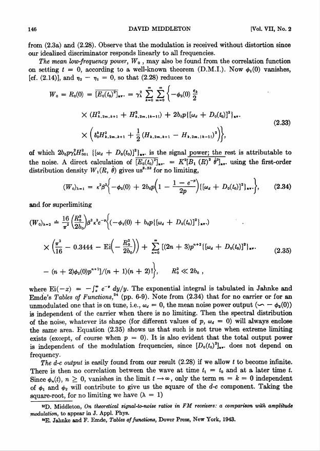
of which 2b0pylH200l {[cod + D0(<o)]2}a»- is the signal power; the rest is attributable tothe noise. A direct calculation of [Z?0(<0)2]av = K2[BX (R)2 d2]ay. using the first-orderdistribution density Wi(R, 9) gives us3,23 for no limiting,

(TFo)x-i = «2/32{-02(O) + 2b„p(l - + «o(«]2}avj, (2.34)

and for superlimiting

(TFo)x-2 = ^(fj-)/3V<r*{(-<*.2(0) + Mt«< + Do((o)]2|„.)

X - 0.3444 - Ei(— ^)) + £ [(2n + 3)p"+2{[co, + D0(t0)]2(2.35)

- (» + 2)<k(0)p" ]/(« + 1 )(n + 2)!>, Rz0 « 2b0 ,

where Ei( —x) = — JT e" dy/y. The exponential integral is tabulated in Jahnke andEmde's Tables of Functions,24 (pp. 6-9). Note from (2.34) that for no carrier or for anunmodulated one that is on tune, i.e., <ad = 0, the mean noise power output (^ — $2(0))is independent of the carrier when there is no limiting. Then the spectral distributionof the noise, whatever its shape (for different values of p, ud = 0) will always enclosethe same area. Equation (2.35) shows us that such is not true when extreme limitingexists (except, of course when p = 0). It is also evident that the total output poweris independent of the modulation frequencies, since [D0(£0)2]av does not depend onfrequency.

The d-c output is easily found from our result (2.28) if we allow t to become infinite.There is then no correlation between the wave at time tx = ta and at a later time t.Since n > 0, vanishes in the limit t only the term m — k = 0 independentof <t>i and <t>2 will contribute to give us the square of the d-c component. Taking thesquare-root, for no limiting we have (X — 1)

23D. Middleton, On theoretical signal-to-noise ratios in FM receivers: a comparison with amplitudemodulation, to appear in J. Appl. Phys.

"E. Jahnke and F. Emde, Tables of functions, Dover Press, New York, 1943.


[ud + D0(O].,.(ir/2) /2PiFi{1/2'i 2; —p),

= + flo((o)].,.W2)V/![IoW + I iip/2)].)(2.36)

in terms of modified Bessel functions (see Appendix IV). The superlimiting case (X = 2)yields

[®o(ô)]»»* — K@Ro[&d ~)~ -Do(ô)]av-P'1^1(1 j 2; P) ,7r

— K0RJut + -Do(ô)]«v(l 6 ").7r

(2.37)

-]•

Both (2.36) and (2.37) are in precise agreement with previous results.3,23 If[wj + Jo(io)],t. vanishes, there is no steady output component. (Figure 2 also illustratesthe square of [E0(<o)Lv , provided we replace {[w* + Z>0(<o)]2}av by [wd + Z)o(<o)]»T. •)

We are now ready to examine the two important limiting cases which occur whenthe incoming carrier is strong, or weak, relative to the rms (input) noise level. Let usconsider first the case when the carrier is strong, i.e., p2 1. The asymptotic expansionof 1 Fx (see D.M.I.) is needed here, namely,

F (a- B- —x) —^ x~a\ 1 4. a(a ft "t~ 1)P> x)_r(/?_a)x [_1 + a.

(2.38)a(a + l)(a — <3 + l)(o? — + 2)

+ 2!x2 +

1. Strong Carrier. For large ratios (p) we find accordingly that

_ T[(k + 2m + n + q + \- i)/2]p-<»"-+-"-»"a; _ &<"+x-1)/22<3—X)/2[m!(m + fc)!]1'2

(2.39)[1 + (k + 2m + n + q + \ — 1 )(fc + 2 m + n — q + \— l)/4 p + • • •]

T[(q + 3 — k — 2m — n — X)/2]

The correlation function (2.28) becomes

B-(1) *> ti-^rK4-'x)/2r <-*«- <• -

+ (x - ifamil + V2) sin (.h - m)].T. (2'40)

-j- (X — l)2^>o(i)['7lT72 COS (172 — »Jl)].v. + 260phi772]aT.}, p2 1.

The first three terms represent (sxn) noise, and the last term is the signal contribution(sxs); (nxn) noise is suppressed. Note that the contribution of the noise enters linearlyin the correlation function: only <p0 and its derivatives appear. This means that theoutput noise is still random in the "pure" sense in which it entered the limiter-dis-criminator elements. In other words, the effects of the transients which gave rise tothe original noise in the IF still add linearly in the output. In spite of this, discrimination


remains a nonlinear process, as the mixing of noise and signal indicates (Eq. 2.40).That the noise can still remain random in the present case is due to the fact that dis-crimination is (for our ideal discriminator) frequency selective and not amplitudeselective: the noise loses its "randomness" (normal properties) only when subject toamplitude limitation, i.e., distortion and/or clipping.

From (2.2) and with the help of (2.14) we may write the output noise spectrumwhen there is no limiting as

W,o(/)x-i — -4k2/S2 [ 02(<)[cos (ij2 - ih)]„. COS oit dt, p2 » 1,Jo

— 4k2(32 ̂ 2 An f cos (7wia + ud)t cos cot dt f («' — o>0)2 (2.41)n = 0 •'O ^0

X w(f) cos («' — oi„)t df, (/' = o>'/2 x),

after expanding [cos (ij2 — fOLv in a Fourier series; here fa( = ua/2ir) is the fundamentalfrequency of the modulation. Integration using the Dirac delta-function6"8 gives us

JFo(/)x-i — k2/32 [ («' — w0)2w(/')[5(<o' — £o0 — nwa — oid — a>)n = 0 JO

+ 5(to' — a>n — nua — ud + co)] df(2.42)

— K2/32 ^»[(^o + Wd + co)2w(a>0 + no),, + COi + co)71 = 0

+ (rko„ + &3<i — co)2w(co0 + + ud — co)].

Observe that the spectral density at and near / = 0 is finite and nonvanishing, nomatter what distribution the input spectrum w has.

The case of superlimiting (X = 2) when the carrier is strong is particularly inter-esting. If we let x = t0 and y — t0 + t, the three noise terms in (2.40) may be written •

So(<)noi.eO«2) ^ ^ *,'S#©P"I{~0,(<) °0S ̂ + I* DM

+ <^i(t)|[2ud + D0(x) + D0(y)] sin (udt + D0(t') dt'

+ 0o(o|["i + D0(x)][cad + D0(y)] cos

i+£)(ft+X cos j^corfi + J Do(t') dt' dx/x0|,

03dt + J Do(to) df'jjm.j

(2.43)16

27T

o (t)


where £0( = 2x/w„) is the period of the modulation and 4>n(t) = {dn / df)<t>0{t). Expansionof the integrand in a Fourier series, followed by the average over x, gives

j I*:c0 J" r*y = X+t J oo— / cos <u>dt + / D0(t') dt' \dx= An cos (nu>a + o)d)(y — x),%o Jo L x J n=o ^ 44)

y — x = t,

since the result must be even in t. The coefficients An are the same as those for thedevelopment in (2.41). Next, we substitute (2.44) into (2.43), which shows that

^ ^4 K2p2(§f)p~l X) An[-<j>2(t) cos (nco„ + oid)t■K \2 bo/ n-0 (245)

+ 2(nu„ + cod)<t>i(t) sin (moa + ud)t + (nua + a)d)2<t>0(t) cos (ruo„ + cod)<].

Use of the integral form of <t>n(t) gives us, finally, a relation similar to (2.41) for thenoise spectrum:

Wo(/)*-2 ^ k2/32(|^-)p-1 X) cos (Wco» + "<*)* cos cot dt

X [ [(co' - co0)2 + (nu* + ud)2]w(f ) cos (co' — coo)t df (2.46)Jo

— 2 ^ (noia + ud) sin (nco„ + ud)t cos wt dt ^ (a/ — o>a)w(f ) sin (co' — w0)t df

ytA-{CK"' co0) + (nwa + C0j) — 2 (ncoa + 0}d)

X (co' — w0)]w(/')[5(w' — o)0 — wco,, — ojj + co) + 5(co' — co0 — wco<. — co<i — co)] d/'

which is

Wo(/)x-2 — ^4 /c2/32(^-)p_1 X) Anco2[lc(co0 + ncoa + cod + co)7T \aOq/ n = 0 ^2 47)

• + w(co0 + nco„ + co,; — co)], p2 )8> 1.

The significant fact about (2.47) is that the spectral intensity for superlimiting alwaysvanishes at / = 0 and is small in the vicinity of / =0. Compared with our result forthe unlimited case [cf. (2.42)], this shows why for a sufficiently strong carrier, limitinggives a noticeable improvement over no limiting, provided we observe the signal components)in a band, near zero frequency, which is narrow relative to the width (^/6) of the (combined)IF-limiter-discriminator filter response, i.e., / <K fb ■ This result is identical with Blach-man's,3 which was derived by a different method, and it agrees with the earlier workof Carson and Fry.1

From (2.40) we observe that for p2 1 the noise is always suppressed, its contri-bution being proportional to p1-x and that of the signal to p2~\ Accordingly, when


there is no limiting, the noise power is constant and the output signal strength increasesas p1, whereas for extreme limiting, the noise actually vanishes as p —* «>, and the signalreaches a limiting value independent of p. These comments are illustrated in Fig. 2.We notice also from (2.40) that when X = 1, the noise power output is independent ofmodulation; this is not true for extreme limiting (X = 2);

2. Weak Signals. When the signal is weak or, at most, of the same order of magnitudeas the noise, the correlation function (2.28) is most conveniently described22 by a powerseries in p; if we use (2.29) and omit terms in pn(n > 3), we obtain finally after con-siderable reduction the following result:

Ro(t) = 7xr(X/2)22X 3&o~X{Cro(<) + p(?i(<) + p2[(?2(<) + 2{j7i7J2}.v] + •** }(2.48)

p3 « 1,

where

G0(t) = (r? - r0r2) 2F1(X/2, X/2; 2; r2), (2.49a)

G,(<) = (r2 - r„r2)|—X 2F1(X/2, X/2 + 1; 2; rl)

+ ra ^ ^1 (X/2 + 1, X/2 + 1; 3; r2)[cos (rh - + ^olvivt cos (r?2 ~ iji)].».

(2.49b)

- n[(i?i + Vi) sin (ij2 - t/OI.v — r2[cos (ij2 - r?1)]av.|2F1(X/2, X/2; 2;r2),

and

(?2(0 - (r? -r„r2)|^2F1(X/2 + l,X/2+ l;2;rJ) + X/4(X/2+ l)-2F1(X/2,X/2 + 2;2;r2)

- ^ (X/2 + 1) 2Fi(X/2 + 1, X/2 + 2; 3; r2)[cos (t,2 - „)]».

+ ^ [cos 2(7;2 - „)]a-[2 2Fa(X/2 + 1, X/2 + 1; 2; 7$ - 2Fa(X/2 + 1,

X/2 + 1; 3;r2)]| + 2Fi(X/2, X/2 + 1; 2;ro){ 77'"o['71'J2 cos (772 — ii)]«».2

+ Xn^Tj! + 7J2) sin (t;2 - 77OU. + r2 X/2[cos (772 - tjO] ■} (2.49c)

+ 2f\(X/2 + 1, X/2 + 1; 3; r2){-^ [(* + *) sin 2(„2 - t,,)].

+ [^1^72 cos 2(772 — TJjXU. — 7-~ [cos 2(772 -

+ 2[t7i772],t.[2F1(X/2, X/2; l;r0) — 1].


The reduction is accomplished with the aid of the recurrence relation

nnTjFtia, b; c; x) - 2F,(a, 6; c + 1; x) = ^ + ^ 2Fj(a + 1, b + 1; c + 2; x). (2.50)

We see at once from (2.48) and (2.49) that the output noise is no 'longer "pure," i.e.,the transients producing the noise no longer add linearly in the output, unlike the caseof a strong carrier and weak noise.

The first term in (2.48) represents the correlation function for the noise outputthat would exist in the absence of a carrier, and 2p2[r)ltj2]S:V. is the expression for theoutput signal or modulation. In threshold perception (p < 1) the observed signal is sup-pressed by the noise and the output signal-to-noise {power) ratio is therefore directly pro-portional to p2 (for the leading term), just as in the amplitude modulated cases.11,13' Thisis true whether or not there is limiting.26 Figure 2 shows the output signal power as afunction of the input carrier-to-noise power.

Part III: Special Cases

1. Noise alone. The first important example occurs when the demodulated wave isnarrow-band noise. Here »7i = i?2 = 171 = ij2 = 0 and p = 0 also, so that the correlationfunction (2.48) is simply.

r> /f\ 2/ 2 nt2—x«x—3 r2mr(m + X/2)2Ro(t) - 7x(ri - r0r2)b0 2 £ m!(m+1), ,

= yl(rt - r0r2)6rx2x"3r(X/2)2 2f\(X/2, X/2; 2; r2).

In the instance of no limiting we obtain

flo(0x-i = I kPMtI ~ r„r2) 2F\(l/2, 1/2; 2;r$),

= kY I (r? - r0r2)K(rl),

(3.1)

(3.2)

where K(rl) is an elliptic integral of the first kind, with modulus r0 . With the aid of

r(Y)r(y - a - fl)iFi(a, P; 7; 1) = r(7 - a)r(7 - j8)'

R(y) 5^ 0, —1, —2, R(7 - a — 0) 0,-1, -2, • • • ,

we find the mean low-frequency power to be

(TFo)x-! = Bo(0)x-i = - «2/3V2(0) = kY f (<* - «0)2to(f) df, (3.3)Jo

*See, in particular, Sec. VII, Part I and Sec. II, Part II, ref. 13."See references 23 and 3 for a discussion of signal-to-noise ratios.


a special case of (2.33) or (2.34) when p = 0. The spectrum follows from (2.2) and (3.1);it is

Woif)^x = irb0K2f}2 ± f [n(tf - r0(t)r2(t)]rT(t) cos »t dt. (3.4)m = 0 Jo

At this point, and 'for all subsequent calculations, we assume a Gaussian spectral dis-tribution for the incoming noise, representing the composite //'-limiter-discriminatorfrequency response, viz.,

w(f) = W0 exp {— (o — cooand b0 = W0ub/2ir1/2, (3.5)

where W0 is the maximum spectral intensity of the noise entering the limiter. From(2.14) and (2.15) we find that

r0(t) = exp {-w2ht2/4}, n(t) = —wbtr0(t)/2, r2{t) = Ji{u\t2 — 2)r-0(f)/4, (3.6)

so that (r\ — r0r2) = a>lr0(t)2/2. Similar relations for the "optical" or single-timed char-acteristic and for rectangular spectra are discussed briefly in Appendix V. Substitutionof (3.6) into (3.4) gives

KW>w - (IP^ ± ^where Q = co/cot = f/fb .

The distribution is shown in Fig. 3.The correlation function for extreme limiting assumes the form

22o(Ox-. = - r0r2) 2^( 1, 1; 2; rl)V260

- 16 2 l[^0 V /'(3.8)

n — r0r21rl > log, (1 - r20).

Although jBo(0)(x-2> is logarithmically divergent, the mean (low-frequency) outputpower is actually not infinite, but zero, since (3.8) applies rigorously when t —> 0 onlyif Rl/2b0 —> 0 also; in other words, the limiting is so extreme that essentially no low-frequency components are produced. All the energy goes into higher harmonics.6 Forcomputation of spectra, however, it is sufficient that Rl/2b0 <SC 1.

We obtain the spectrum (X = 2) at once from (3.1) or (3.8) and (2.2) for the Gaussiandistribution (3.5). We have

TTr ff\ ■ 32 (Rl\22 r v exp {- a2/(2m + 2)} , .TFo(/)x=2 - [WJ« P £ (m + 1}3/2 • (3.9)

Figure 3 also illustrates W0(f)\-2 as a function of 0. The spectral intensity at 0 = 0 is

T^o(0)x-2 = ^ (|j-)/3V<oAf(3/2), (3.10)

where f is Riemann's zeta-function26 and f (3/2) has the value 2.612. Some details ofthe evaluation of (3.7) and (3.9) are available in Appendix V. From (A5-2) it also

26Jahnke and Emde, loc. tit., pp. 269-273.

1949] • SPECTRUM OF FREQUENCY-MODULATED WAVES 153

follows that when 0 becomes infinite, the spectral intensity (3.9) falls to zero asl^oCOx-2 — 16/32K20)i,i2o/'T 0(0 —

2. Tuned, unmodulated carrier. The unmodulated carrier in noise is the next morecomplicated case. Now = r]2 — 0 and Vi — V2 — 0 also, provided the carrier is tunedto the center of the band, i.e., 01,, — 0. The correlation function (2.28) then becomes

Ro(t) = 7x Zw Er„(i)2"+t{-^«)(ffu„,i+i + Hl.2m, 1^,)= 0 6 OT = 0 I

(3.11)

~f~ <£l(0 (Hk,2m + \,k 2 Hk,2m + l,k + 2 Hk . 2m +1, I ib-2 I

with j) = Aa/2lj:i as before. The power output associated with the low-frequency termsis obtained at once from (2.34) and (2.35), viz:

(W0)x., = -V/J^O),(3.12)

* - 7(t>v*-(0)n?5 - ®(-1;) - °-3444 + § fr + UK. + DJ•Observe that the mean-square low-frequency output of the ideal discriminator is inde-pendent of carrier strength when there is no limiting. This is what one would expect,since the carrier is timed to the central frequency of the symmetrical band, and itsd-c therefore vanishes.

The mean power spectrum follows as before from (2.2) and (3.11). For the Gaussianinput noise distribution it is

2m + k + 2m +X + 2)(Hl-2m-k+l

« +1

Wn(f) = 7x2V/2o>A^ E % Efc=0 £ m=0

2 . exp {- Q,2/(2m + k + 1)} , / 202 . , -+ i*-i, ) (2m + fc + X)3/2 + °y 2m + fc + 2/ ( ' '

2 _ 1 tj2 _ 1 tt2 \ exp { — O2/(2m + fc + 2)}k,2m + l,k 2 fc,2m + l, fc + 2 2 ^ +1» I 21 y ~/c "j- 2)'*^

The spectra for no limiting are shown in Fig. 4 for various values of p, and for super-limiting in Figs. 5 and 6. The significance of the results is discussed briefly in Part I.

When the carrier is large, the spectrum is foimd at once from (2.42) or (2.47). Theseresults give the leading term, while a further use of the asymptotic development (2.39)gives the succeeding one. Here

A„ = 5°

and w(f) = 2b0cob1Tr1/2 exp {—(co — co0 )2/«&}> so that

Wo(/)x-i ^ 4ir1/V/32fo0w,,jfl2 exp (— A2) - ^ , (3-14)0 exp (— 0 )

4-21 (1 + O2) exp { -n2/2} + ■ • • I V » 1-


A similar procedure for superlimiting [cf. (2.47)] yields

Wo(f\,2 ~ 4^ K2p(^Qb0o,b i jo2 exp (- fi2) + eXP 2^2/2i + •■•}• (3-15)

The mean output power corresponding to (3.12) when p2 1 is simply — k'when X = 1 and is

(WA-, - [ W.(/V, i/ - 4 7 {l + ^ + ' • • <316>We notice that when there is extreme limiting (R20 <SC 2b0) and the carrier is strong(p2 5>> 1), suppression of the noise occurs, analogous to the similar situation in the re-ception of amplitude-modulated waves.11'13 The spectra for the strong carrier case areillustrated in Fig. 6.

The small-signal problem, on the other hand, gives us a different output spectrum.From (2.2), (2.48), and (2.49) the spectrum of the noise may be written

Wo(f) = 7xr(X/2)22x-1f>2-x f [G0(t) + pGJt) + p2G2(t) + • • •] cos ut dt, (3.17)*'0

which in the instance of the Gaussian distribution (3.5) becomes finally

w0(f) = ^„(/)noi8ep° + 7^r(x/2)W1/22x-2&rx

[ -X(\/2)m(X/2 + 1), exp {-02/(2m + 2)}1 tha m\(m + 1) !(2m + 2)1/2X \v

2(X/2)2(X/2 + l)j exp { - 02/(2m + 3)1m\(m + 2)!(2 m + 3)1/2

(X/2)2m\(m + l)!(2m +1)

exp { —fi2/(2m + 1)}

7 202 \_1,\ 2m + 1/ (2m + 1)

+ P2_ 771 = 0

x2/x , ,v , x /x4 V2 + + 4 V2 + 1 +2)„

+ 2MDtt + 'Iferi)](3.18)

exp { — O2/(2m + 2)}m\(m + l)!(2m + 2)1/'!

(X/2)2(X/2 + l)(X/2 + l),(X/2 + 2), exp { - Q2/(2tw + 3)jm\(m + 2)!(2t?i + 3)1/2

(X/2)(X/2)m(X/2 + 1).m\(m -f 1) !(27re + 1)1/2 1 " 2^Tt) (2m+1) " exp l-tf/fa- + Dl

(X/2)'(X/2 +1)1 ( tf \ _ a "I 1,m\(m + 2)!(2m + 2)3/2 V1 m + lj 6Xp 1 " /{Zm + Z)] J + J"


The curves of Figs. 4 and 5 for p < 0.3 have been calculated with the help of (3.18).223. Off-tune, unmodulated carrier. This is a generalization of the preceding case to

include the effects of a constant deviation of the carrier from the /F-limiter-discriminatorresonant frequency/0 . It is now evident that iji = &>dt0 , ij2 = uJh + t), and so vi =t)2 = ud . The correlation function (2.28) reduces to

Rod) = 7x E £ rlm+k{ -021 (m,2m,t+1 cos (k + 1 wt = n m. = 0 I & \

+ Hi, 2m, | k- -ii cos (1c — 1 )wdtj

~h 01 2 b,2m + l ,k COS 2 H iCi2m + l,k + 2 COS (/b 2 )c0d^

U20 "fc,2m + l, | fc —2 | COS (k - 2)wdtj (3.19)

+ (26oP) 7 ^(1 ^o)Hic,2m,k+l(Hh,2m + l,k + 2 Hk,m + \,k) SU1 (fc l)cCdt

Hk.2m,\k-l[(Hk,2m+l,k Hk, 2m + 1, 11_ 11) Sm | fc 1 |

+ 2b0Wdp COS + ~^(Hk,2m,k + \ ^it ,2m, I A-l l) ^ J*-

The effects of the carrier with constant deviation are discussed in Part I. The contri-bution of the signal component is illustrated in Fig. 2, where it is seen (from the ordinatescale) that the signal power varies as the square of the deviation fd. The general determi-nation of the noise spectrum may be made in the usual way with the aid of (2.2) and(3.5).

The example of a strong carrier is instructive. Then, with the Gaussian distributionas a particular example, we see from (2.42) and (2.47) that when there is no limitingthe output spectrum is

TFo(/)x-, ^ 2irI/V/32<oA[(0, + fl)2 exp {-(a, + Q)2}

+ (fl, - Q)2 exp { — (0d - 0)2}], Ud =(3.20)

since here the Fourier development of [cos (r?2 — *h)Ly. is simply An cos wdt, An = 5° .The mean output power is (uhK$)2b0/2, which is proportional to — #2(0), and is inde-pendent of modulation, which in this case is the deviation of the carrier from resonance.This can be observed at once from (2.40) or directly by integration of (3.20). Figure 7shows the spectrum (3.20) for various ratios .

The spectrum after extreme limiting is found in a similar manner to be

TF„(/)x-2^^ exp {-(12, + fi)2} + 02 exp {-(£2, - O)2}],

(3.21)V » 1.

156 DAVID MIDDLETON [Vol. VII, No.'j2

Fig. 7. Low-frequency noise spectrum following discrimination, for a weak noiseand an off-tune carrier and no limiting.

Figure 8 illustrates the spectrum in this instance. The mean power output of the dis-criminator may be obtained from

OFo)x_2 - 41 J n2[exp {-(a, + Q)2} + exp - 0)2}] dSl

— ^ (K/3o)t) {2bJ p + 2j,

2tt(3.22)

showing that the noise depends on fi2 , as can be seen from Fig. 8.The distribution in the neighborhood of / = 0 is easily determined with the help

of Taylor's series

exp {-(0, ± S2)2} = (2tt)1/2 £ (±1)' @5j!%(,)(2l/alU;

(3.23)(ovn f — O2 \ ^

(2*-)1/2 d(2U2ady<t>U) = m-lw ,, (exP {— o3}),


5.0

4.0

3.0

2.0

1.0 2.0 3.0 ft 4.0

Fig. 8. The same as Fig. 7, but for extreme limiting.

a development which is valid for all fl and Qd . Equations (3.20) and (3.21) are accord-ingly modified to

W0(/)x-i ^ 4:r1/V/32a,A{$ - 20firf + fl2(l - 5 ft + 2flJ) + ■ • • } exp { —Oj},(3.24)

fi3 « 1

and

TFo(/)x-2 ̂ % kY^Kp-1^{fi2 + • • • } exp { - . (3.25)


A comparison of (3.24) and (3.25) bears out the general observation made followingEq. (2.47).

w (fl. )/ (2 JtT k2/3 2 b0u> b]0.75 |-

p = 0

0.5 -

0.25 -

0

"o2.0 h-

n

P'O

0.5 -

(b)Fig. 9. Typical low-frequency spectra for an off-tune carrier: (a) no limiting,

(b) extreme limiting.

4. On- and off-tune carriers modulated by a sine wave. In this case we have

77 = oid + D0 cos o)at, and v — Udt + M sin uat) n = —2 = (—°)'7r- (3.26)\03b / "o

Here n is the modulation index, and D0 is the maximum deviation of the modulation,while o)a is its angular frequency. (For such modulations the inequalities D0 « o>0 ,


coa <5C co0 must hold.)9 Referring to the general correlation function (2.28) we see thatthe modulation enters by virtue of the coefficients

[cos 1(ti2 — 7h)].v. , [(»)1 + V2) sin l(r)2 — iji)]aT. ,

and [77^2 cos Z(i?2 — >h)]av •

A straightforward application of the techniques of Appendix III allows us to writethese averages as

[cos l{t)2 — »?i)]av. = X) e'nJn(l/i)2 COS (ruo„ + lad)t, (3.27)n = 0

[(171 + V2) sin l(ri2 — tj,)J„. = ^ enJn(ln)\~- Jn-i(ln) sin [(n — 1)«„ + lwd\tn = 0 I ^

+ 0}dJn(lfi) + + + «^n-l(M)j sin (ruca + lud)t

(3.28)

4—^ Jn+ i(W sin [(n + !)&)„ +

and

[V1V2 cos l{i)2 — »h)]a £ e„/n(w{[^p + Y Ulfi\

X cos [(n. — l)w„ + kod]t

+ + ^r4 (J„+1(W + J„-i(W) + ^ (/n+2(W (3.29)2

+ J„_3(Zm))J cos (nua + lwd)t

+ h (2m)]Jn+1(W + Y /„(&») 1 COS [(n + l)Wo + h>d]t).

When the carrier is tuned to resonance, ud vanishes and (3.27) to (3.29) simplify con-siderably. However, a precise determination of the spectrum in either instance (ud = 0,or i»i 9^ 0) is a very tedious process. Fortunately, for many purposes the qualitativeand semiquantitative conclusions obtained from the limiting behavior of the generalcase are sufficient; (see Part I).

We note that for strong carriers (p2 5>> 1) the output spectrum may be found asbefore from (2.42) or (2.47). Equation (3.26) shows that the Fourier expansion of[cos (t]2 — j?i)]av. is An cos (noia + wd)t, where A„ = e„./„(/x)2, so that for no limitingand our usual Gaussian noise distribution we find

Fo(/)x_i ^ 27Tl/V/rW>„ z + nd+ a)2 exp {-(nsia + nd + o)2}k (3.30)

+ (nQ. + nd - Q)2 exp {-(nfl. + 0, - O)2} >, fi0 = —,J "i,


and the mean output power is simply (k2/32<4)60/2, [cf. (2.40)]. For superlimiting weobtain

Wro(/)x-2 ~ 41 K2p2cobb0(^^p 'n2 <;n-/n(M)(exp {-(nO, + 0,, + 0)

+ exp {— (nUa + % — Q)2

CO 24 a es

Fig. 10. Low-frequency noise spectra following discrimination, for a weaknoise and a sinusoidally-modulated carrier on tune.

(3.31)


The mean output power associated with the noise in this instance is

+

(3.32)

(TF0)x=2 = [ W0(f)>_2 df

+ £ + 2naaad)J2Mj.

Figures 10 and 11 illustrate the variation in spectra for different modulation indices andmodulation frequencies in the somewhat less general case of zero displacement fromresonance, ttd = 0.

a

Fig. 11. The same as Fig. 10, but for extreme limiting.


APPENDIX I: Second-order probability density, its characteristic functionand associated moments

Let Xk (k = 1, 2, 3, • • • , s) be s random variables, each of which in turn is the sumof a large number (N) of independent random variables xik (i = 1, 2, 3, • • • , N), dis-tributed according to some law. Then the central limit theorem27 states that the dis-tribution of the X's is normal (i.e., multivariate Gaussian) in s dimensions, subjectto certain restrictions [see e.g. S. 0. Rice,27 Eqs. (2.10-3)] on the distribution of theXik's comprising Xk , restrictions which are assumed to be satisfied here. The probabilitydensity of the Xk's is

. exp { — XM X/2)<)- [(2r).ur

(Al.l)

where M is the reciprocal matrix to m, with elements y^'/l I/**' is the cofactor ofHu ; I m [ is the determinant of n, and X is the transpose of X. The matrix u is symmetricaland has elements

2V

Mfc! = Xik%il > (A1 .2)*

in which xik is the i-th element in the sum comprising Xk and xit is a similar elementin Xi . We assume here, without loss of generality, that Xa xiH = 0, i.e., that Xk — 0.All odd moments are therefore zero. The Fourier transform of W2 (Xi , • ■ ■ , X, ; t) isknown as the characteristic function and is8

F2(zi , • ■ • , z. ; t) = exp j^- | £ J2 MuZtZiJ. (A1.3)

Now, in particular, we denote here the various "in-phase" and "out-of-phase"components Vel , ■ ■ ■ , V,2 and their derivatives Vcl , ■ ■ ■ , V,2 [which by (2.6), (2.7)and the properties (2.4) are random variables] by , • • • , Xs , (s = 8). The subscript1 on Vc , Vc , or Vs , V, refers to an initial time and the subscript 2 to a time t later.The elements of our matrix u may be computed as follows, from (2.6) and (2.7) in(A1.2). For example, in the instance of /j„ we obtain

Mil = VclVc, = j J2 (an COS 0)% + b„ sin u'nt0)I n= 1

(A1.4)N 1 __ /•»

X X) (fflm cos u'mta + bm sin ^m^o) | stat* av« D (a2 + b2n)/2 w(f) df,n= 1 ) n= 1 ^0

with the aid of the characteristic properties (2.4) on passing to the limit N —»• co. It is

"Sec S. O. Rice, Bell Syst. Tech. J. 23, 282 (1944), sec. 2.10. D. M. I. also contains a discussionof some of these questions—Appendix I.


assumed throughout that w(f) is such that the various integrals involving w(f) con-verge. All 64 moments (nkl = iilk, p.kl = nu) are similarly found to be

M11 = Vcl = M22 = Fc2 = M33 = F,i — M 44 = F,2 — i>0

M55 = FC1 — M66 = VC2 — ^77 — Fsi — fig 8 = F s2 ~~ b2

Ml7 — FclFsl — H28 — Fc2Fs2 — ^35 — VslVel — /*46 — Fs2Fc2 — ^1 J

13 — VciVsi — 4 — ^02^02 — MlS — FclFc

— M37 — Fs- 1 F,,. 1 — M26 — Fc2Fc2 — M48 — Fs2Fe2 — Oj(A1.5)

Ml2 — VclV c2 — M34 — ^ si ^' s 2 — $d(0>

M14 — FciFs2 — M23 — Fc2Fsl — X0(<) J

Ml5 — FciFc2 — M38 — FslF„2 — M52 _ — FC1 F.-2 _ —M"4 — — FslFs2 = 4>l(f)

Ml8 — VclVs2 ~ M27 — Fo2Fsl — M54 — F<dFs2 — — M63 — — Fc2Fsl = ^l(Oj

M56 — FcIFc2 — /*78 — F,lF»2 — <f2(t) j

M08 — FclFs2 — /*67 — Fc2Fsi — X2(£) •

Here we have

b„ = f (to — too)nw(/) d/, 0„(<) — — \ w(f) COS (to — <0o)< rf/,•'0 3< •'0

(A1.6)X„(<) = —n I w(f) sin (to — to0)< (//.

dt Jo

When the input spectrum w(f) is symmetrical, X„(<) vanishes, as does alsohi+i (j = 0, 1, 2, • ■ •)• The probability density (Al.l) in such cases is given by

W2(VC1 , ••• , 7.2 ; t) = (2ir)~4 | M |-1/2exp 1 VTC + F?2 + V2.i + F,22)2 | n

+ m33(^2i + Vc2 + V2.i + VI2) + 2M12(FclFc2 + FalF,2)

(A1-7>+ 2//4(FclFc2 + F,iFs2) + 2^13(VclVcl + FalFsi — Fc2Fc2 — Fs2Fs2)

+ 2M14(FclFc2 + F.jF., - Fc2Fc1 - F.2Fr.o}].

(A1.8)


The determinant | n | and cofactors // ' are

| M I = Kb0b2 - tf)2 + (0i - 2 - («f + bUl + bl<t>l)f

H11 = I n |1/2[&o(^2 — 0a) — £>a0iL ai12 = I AI |1/2[—— 0o(&2 — 0a)],

M13 = — I M 11/201 [00^2 + &O02], M14 = — | M |V20l[0O&2 + 0002 ~ 0l],

M33 = I M - 0o) - bo0?], M34 = I M |1/2[02(b§ - 0?) + 0i&o],

The characteristic function (A1.3) is represented by (2.13). When the spectrum w(f) isnot symmetrical, the resulting expressions for W2 and F2 are correspondingly moreinvolved, containing in = 0, 1, 2). Specifically, the characteristic function is now

F2(zi , • • • , z8 ; «) = exP (— | j&o(z? + 4 + z\ + z\) + b2{z\ + z\ + z? + zl)

+ 20o(«)(ziz2 + z3zi) + 20I(i)(z1z6 - z2z5 + z8z3 - z4z7)

(A1.9)- 24>2(t)(z5z6 + z7z8) + 2x0(<)(ziz4 - z2z3) + 2x1(<)(zizs + z2z7 - z3z6 - z4z5)

2A,(i)(z5z8 ZgZ7) j j.

APPENDIX II: Evaluation of and K2 when i?0—>00

The integrals K, and K2 (Eq. 2.20) apparently are divergent when there is nolimiting (/i = 1/2 or X = 1, and R0 and it is not immediately evident that theresults of integration (2.21) still apply in this case. The difficulty may be removed ifwe return to the general form (1.11) for arbitrary clipping. Our expressions for Ky andK2 accordingly become

*■ - - 7 L 0" dx //_w xji(X(a;2 + y2)1/2)

dx dy

(A2.1)

2 , 2 exp \-ixz - iy£\x + y

and

K.--Z liin [ (' ~ ![' dx dy* (fto-co) J C \ A / J J -co

vJMf + f)'") %i|.x + y

(A2.2)


Transforming to polar coordinates gives us for Kx

;pw\ radr J,(Xr)i?-! = — — um [ (i - expj-*/uiu r

ft (R JC \ A / Jq

(A2.3)X

where

r2r/ cos 0 exp {z'Zr cos (0 — \j/)\ dd,

cos yp — ^2 _|_ ^2y/2, sin \p — ^ gy/2t and Z — (z + £ )17 >0.

We employ next Eq. (1.4), so that (A2.3) is found to be

K, - - | I (' " exPxi"'filM)[f W-W.W * dX. (A2.4)

The integral in r is a special case of Weber and Schafheitlin's integral10 and has thevalues

f Ji(rX)Ji(rZ) dr = ^.^,(1/2, 3/2; 2; X2/Z2), Z > X > 0

^•^(1/2, 3/2; 2; Z2/X2), \>Z> 0

(A2.5)

At Z = X the functions are identical, viz., 2r(0)/x, but logarithmically divergent.Since this divergence is only logarithmic, the integral in X is still convergent, includingthe point Z = X, and this independently of R„ . We observe now that (A2.5) may beextended to negative values of X if we replace X by | X | and multiply the expressions(A2.5) by ( — 1). The integrands containing the real part of (1 — exp [—z'floA]) thencancel, and we are left with

K, = - ~ limA (R O-CD)

b [ SJIirL aFi(1/2,3/2; 2; x2/z2) dx(A2.6)

+ £ I 2^(1/2, 3/2; 2; Z2/X2) rfx].

Utilizing the fact that lim..(sin R0\)/\ is a delta-function,6'8 with the value7r5(X — 0), we have finally

K - _ 2wiz / A Q 7\Al ~ Z3 ~ (z2 + ?)3/2' {AZJ)

the second integral in (A2.6) vanishes because of the property ft f(x)S(x — 0) dx = 0,b > a > 0. A corresponding expression for K2 is obtained on replacing z by £ in the nume-rator of (A2.7). If we set n = 1/2 in (2.21) we see that the result is precisely that givenabove, cf. (A2.7).


APPENDIX III: Integration for R(<).v

The Bessel expansions for the trigonometric exponentials in (2.27) are

exp {— 4>0p-ipi cos (02 — 0i) + iA0pi cos (0i — th) + iA0p2 cos (02 — jj2)}

00 00

= EE Z(-l)kt*IMoP1P2)l+neltnJ,(AoPl)Jn(AoP2) (A3.1)*=0 1=0 n=0

cos Jc(d2 — 00 cos l(9i — Th) cosn(02 — v*)-

The integration over and 02 indicated in (2.27) is accomplished with the help of

A r" (sin *k'si" *m) H - £/«. and i f" h *") ^ - 0. (A3.2)2tt Jo Vcos i/'fc-cos t^m/ 27t \cos ^K-sm \j/mJ

We at length obtain the following five expressions for the average over 0! and 02 :

C(„ = cos (wr,2 Z5O [a*+ij*+i + 8j»-ii4i»-ii] (A3 3)2e;€„

(t, _ cos (ny2 — ly 1)2e;en

r<<l> _^ 2,In —

1 r 1 fc—21 *. 1 &—212 5" J'lkX - \ s"i+28kn+2 - £ 21 21 I, (A3.4)

Cik.\n = -±- [5„fc+1(5r2 + 5?) cos Vl sin (nv2 - ZuO4«(€„

+ 5*+1(5?+2 — 5^) sin ?ji cos (rnj2 — Zj?,) — 5*~15l*~1|+1 sin ?nj2 cos (Z — 1)771 (A3.5)

+ 5^-ll5? cos ny2 sin (Z — 1)77! — 5*"1 sin n7j2(^l~11-1 cos rh cos Zt?!

— 5|1-11-1 sin rj! sin h+ 5^-11 cos nrj2 (S?-2 cos 57! sin hn + 5j4"21 sin rcos Z^i)],

C"«. = ~r~ [rf+W + Sn) cos „2 sin (n,2 - lVl)4«,en

— 5j+1(5*+2 — 5*) sin y2 cos (ny2 — lyO

+ 5j"15li:~1| + 1 sin Z?ji cos (n — l)y2 — cos Zt7X sin (n — \)y2 (A3.6)

+ b)'x sin lrii(.Slk~1]~1 cos y2 cos ny2 — Sj*-11-1 sin y2 sinn?j2)

— cos lyi(8*~~2 cos rj2 sin ny2 + 5i*~21 sin y2 cos nrj2)],


and

^ [cos „2 cos n* cos Vl cos lVl(8kn+1 + C"ll)(«Tl +

+ cos J)2 cos nrj2 sin 17! sin lvi(8k+1 + 5i*_1')(5t+1 — 5;_1)

+ sin rj2sinmj2 cos cos Zih(5*+1 — <>*~1)(5;+1 + Si*-11)

+ sin t)2 sinnr/2 sin 77, sin Zt7i(5'+1 - 8h~l){81\*1 - ^-1) ^ ^

+ cos 7/2 sin «t72 cos ?/a sin Zjh(5*+1 + 5*_1)(^+1 + 5;_1)

+ cos tj2 sin wj;2 sin 77! cos lTh(8k+1 + 5^_1)(5ife_l 1 — 8k+1)

+ sin 7]2 cos nr)2 cos vi sin — S*+1)(5(+1 -f S^-1)

+ sin 772 cosruj2sin ^ cos lvi(8[nk~li — 5^+1)(5|fc~l 1 — 5*+1)]

with the convention that 8^" = — . The correlation function may now be written

Ro(t)N = yl it £ £ €^!€„(-1)'+(,+b,/2 f pxr'J,(ptA0) exp (—60p?/2) dp,ifc = 0 I= 0 n = 0 ^0

X / P2 ii(P20) exp ( b0p2/2)Ik(<t>0p1p2) dp2Jo (A3.8)

X + (t>2iPiP2C{2k,\„ + iAo^iT/iPiC^L + iA0<l)1rj2p2Clk]n — Aoih^C^u} •

The series in n and i are eliminated because of the Kronecker deltas in (Z, /c) and (n, k),which appear everywhere in pairs in the various C's. If we separate the variables piand p2 by expanding [k(4>nplp2), integrate, and reduce the C's, we finally obtain (2.28).

APPENDIX IV: Some properties of Hk,2m+n,a(p; X)

The determination of spectra requires a wide range of values of the order(k, 2m + n, q) of the amplitude functions Hki2m+niQ(p; X). These values are best foundwith the help of recurrence relations, which greatly facilitate the work of computation.The amplitude function H is described by (Eq. 2.29)

r[(fc + 2m + n + q + X - l)/2]p°/2nk,2m+n.AP, AJ ~X)/2[ra!(m + k) !]1/2

(A4.1)X 1Ft([fc -(- 2m + n + q + X — l]/2; q -(- 1; —p),

k, m, n, q > 0 and integral. Here q is equal to k plus an integer, and n is either zero orunity. Using this fact we distinguish, for convenience, two classes of functions, denoted


respectively by superscript zero and superscript unity. The amplitude functions arethus only of double order (in k and to).

Recurrence relations between the H's are readily found from those of the confluenthypergeometric function 1f, , a table of which we list below,28 after multiplication bythe appropriate factors [cf. (A4.1)]. We have

1.

2.

3.

4.

5.

6.

-0

±p(0 - a)

±p(0 — a)

F13-

1 -

0 - 1

0(0— 1)

2a =F V

-0(ot ± p)

(0 — a — 1)

1 — a =F p

0(1 - 0 =F p)

(A4.2)

The subscripts on F heading the columns refer to an addition or subtraction of unityin a or 0 of F = iF^a] f}; ±p), the rows list the factors which multiply the headingF's, and the upper sign wherever (±) occurs refers to lF1 (a; (3; +p), while the lowerrefers to iFi(a; /3; — p). The sum of each row is zero.

There are five distinct H's, corresponding to <7 = /c + 1, [ /c — 1 j, with n = 0, andq — k, k -\- 2, \ k — 2 \, with n = 1. For each amplitude function, two recurrence formulasare needed to cover the complete manifold (k, m): one for k fixed, m — 0, 1, • • • , theother for m constant, k = 0, 1, 2, • • • . Since m appears only in a of iFx(a] 0; —p) [see(A4.1) above] the first row of (A4.2) may be used directly in the former case, viz:

[(/3 - a),Fj(a — 1; /3; —p) + (2a — fi — p)1F1(a; /3; —p)]/a

= + 1; 0; -p). (A4.3)

In the latter, where k is varied, both a and /3 contain k additively, and so we seek arelation between F, Fa-^ , and Fa+p+ . Now if we change 0 to /3 — 1 in 4. of (A4.2),and again alter a to a +1, use 5. and eliminate Fts_ and Fa+ from these three relations,we obtain

{—08 ~ l)iFi(a - 1; /J - 1; -p) + (0 - 1 + p)1F,(a; -p)}pa

= 1F1 (a + 1; /3 + 1; —p).

28See Appendix 4 in ref. 7.


The general recurrence formulas follow from (A4.3) and (A4.4), and are

1 / fk + 2m + n + X — 1 — q[(to + 2)(to + 2 + k)]1/2 \ ~ V 2~~

x (k + 2m + n + q + X - 1 j rr(n)fc . 2 wt + » , q

[(to + 1)(to + fc + 1)]

+ (2to + n + k + X — p)Hl"f lm + n + 2,a\ = jffi?2m + » + 4,0

(A4.5)

and

1 j ^k + 2 to + re + <? + X — l\ //r(«)

v 1/2(to -f fc + 2) I V 2 / (to + & + 1)

(g + P + 1) rrfn) \ (A4.6)1/2 "fc + l,2m + nffl + l fP

- TT(,n'>"fe + 2,2m+n,fl+2 •

We observe from (A4.1) that a = (k + 2to + n + g + X — l)/2 is either a positiveinteger or half-integer. When a is a half-integer we use 29

+ 1/2; 2M + 1; ±p) = + 1} exp {±p/2}/,(±p/2). (A4.7)(±p)

This is a convenient form for computation because of the available tables of e~'I0(x)and e~JIr(x)21 When a is integral, may be expressed in closed form as a polynomialin p and e~". In general, four fimctions must be known initially for n = 0 or n = 1,in order that (A4.5) and (A4.6) can be used to give us a complete set of H's.

The initial functions 30 to be used in the recurrence relations when n = 0 (q = k + 1)to give us are

HZiv, X) = «xPV2^i(X/2; 2; -p) = alP1/2e^/2[IQ(P/2) + /,(p/2)], (X = 1) (A4.8a)

= a2p~1/2(l - e~v) , (X = 2) (A4.8b)

= ^fVl/\Fx{\/2 + 1; 2; -p) = a1p1/2e-B/2[Z0(p/2) - /1(p/2)]/2 (A4.9a)

= a2pU2e-", (A4.9b)

HZ = ~P >F,(X/2 + 1; 3; -p) = axe~vnIM2) (A4.10a)

= a2(l — e~" — pe~")/p (A4.10b)

29Ref. 21, pp. 191.30W. R. Bennett, J. Acoust. Soe. Amer. 15, 164 (1944).

170 DAVID MIDDLETON [Vol. VII, No. :

and

H™ = (A/2 + 1) ̂ ftr* V /,(X/2 + 2; 3; -p)

= aie-^[PI0(P/2) - (p + l)/1(p/2)]/23/2 = (A4.1 la)r

= a2pe-p/2u* J (A4.11b)

where ax = r(A/2)/6^_1)2(3"X)/2;

in particular, = 7t1/2/2 and a2 = (260)~1/2. (A4.12)

A similar technique is applied to obtain (n — 0, q = | fc — 1 |). Whenfc = 0, i?o°2m,i may be obtained from (A4.8-A4.ll) above. The initial functions hereare

Hill = ax ̂ (A/2; 1; -p) = a^I^p/l) (A4.13a)

= a2e~p, (A4.13b)

^20 = iFi(X/2 + 1; 1; -p) = aie-*/2[(l - p)7„(p/2) + p/1(p/2)]/23/2 (A4.14a)

= 0,(1 - p)e"721/2, (A4.14b)

#S1 = |^p1/21FI(A/2 + 1; 2; -p) = a1p1/2e-r/2[/0(p/2) - 7,(p/2)]/23/2 (A4.15a)

= a2p1/2e~ 721/2, (A4.15b)and

= (A/2 + 1) p1/21F1(A/2 + 2; 2; -p)

•D1/2e"p/2a, V^tt [(3/2 - p)/„(p/2) + (p - l/2)Z1(p/2)]2-6

= 2o2p1/2e_1,(l — p/2)/6

= ^7T^ (A4.16a)Cx

(A4.16b)We continue in the same way to obtain (n = I, q = k). The initial func-

tions are

H(oll = cx 1F1(A/2; 1; -p) = Cle-"/27„(p/2) (A4.17a)

= 026"", (A4.17b)

-V —p/2

7^030 = 2 iF^A/2 + 1; 1; —p) = [(1 - p)7„(p/2) + p71(p/2)] (A4.18a)

= c2(l — p)e~v, (A4.18b)


1/2-P/2

H\\\ = X/2 <xpu\FM2 + 1; 2; -p) = Cl [/„(p/2) - /,(p/2)] (A4.19a)

= c2p1/2e"J', (A4.19b)and

//,<>> = (X/2 + 1) jpT? p1/2iF1(X/2 + 2; 2; -p)

1/2 —p/2

= P P/2 - p)/o(p/2) + (p - l/2)J1(p/2)] = 3I/2^;i (A4.20a)

= 2c2p1/V(l - p/2)/21/2, (A4.20b)

and here

Cx = r(X/2)/bo/22<2_X)/2; specifically, c, = (ir/260)1/2 and c2 = b^. (A4.21)

There remain *=+2 (n = l,q = k + 2) and Hi] L+i.it-21 , (n = 1,1 = I k ~ 2 I)-For the former we find the initial functions to be

Holl = (X/4) c\p-1F1(\/2 + 1; 3; -p) = c<T*nIx{Vl2) (A4.22a)

= c2(l - e-p - pe~")/p, (A4.22b)

^032 = (X/2 + 1) ^p-^X/2 + 2; 3; -p) = c, ^ \ph(p/2) - (p + l)/,(p/2)]

(A4.23a)

= c2pe~p, (A4.23b)

-P/2

\ —P/2

ff'ii = (X/2 + l)|p3/,/1(X/2 + 2; 4; -p) = ^75 [(4 + p)7I(p/2) - pj0(p/2)]

(A4.24a)

= c2p~3/2(2 - 2<T* - 2pe-p - pV),(A4.24b)

and= -(2 + X/2)(q1 ̂ /2V2)Xp3/2Cx >^(V2 + 3; 4; -p)

o • Z

_-l/2^-p/225/2

p-1/2e-"/2[(2p2 + p)70(p/2) - (2p2 + 3p + 4)7,(p/2)] (A4.25a)

= c2p3/V72,/2. (A4.25b)

l*-2| jWe have finally, for Hiv2m+x,

77<;> = ^ iT1 i(X/2 + 1; 1; -p) = [(1 - p)7„(p/2) + p7,(p/2)](A4.26a)

= ^22 (1 - p)e~", (A4.26b)


I "h

axQJ

•<s»

£

CQ

<NH

Q,X03

<NH

DhX03

«|<N

3_J

(M

OhXo>

D,xo

I1ft I

.3XJl

I

+0

V

V•©

1o

S—v,

©

IH.a

H.3

A

I

as<3

as

V•o

+

oAH

H

O

Ao— H

I IQ,X03

toM -O

3I

H

Tax03•o3I

o oA IIH H

©

H

Tax03

3I

^3

+

"<S>"S,o


\r -p/2Hill = (X/2 + 1) ̂ 72 iFi(X/2 + 2; 1; -p) = [(p2 - 3p + 3/2)/„(p/2)

(A4.27a)+ (2p - p2)J,(p/2)]

= ^ (2 - 4p + p2), (A4.27b)

■v 1/2

Han = (X/2 + 1) 1^75 lF1(\/2 + 2; 2; -p)

= f^<TP/2[(3/2 - p)/„(p/2) + (p - \/2)h(p/2)\ (A4.28a)

= 2c2p1/2e-p(l - p/2), (A4.28b)

and

= (x/2 + 2)(X/2 + 1) ̂ 75 pu\Fx{\/2 + 3; 2; -p)

r rt1/2p~"/2= ^17- [(P2 - 9p/2 + 15/4)/„(p/2) - (p2 - 7p/2 + 3/4)71(p/2)] (A4.29a)

i/2 -®

= • 6'6/2 ̂ ~ 6P + 6)- (A4.29b)

APPENDIX V: Evaluation of Series (Noise alone);

Remarks on Optical and Rectangular Spectra

We note here some possible methods of summing the series (3.7) and (3.9) in theinstance of noise alone. For no limiting (X = 1) Rummer's transformation31 puts theseries (3.7) in a form that is more rapidly convergent. Here we writeAm = 2(m + 1) exp {/S/(m + 1)}; am = (1/2);; exp {—0/(m + l)}/(m!)2(m + 1)3/2;

20 = <o2/a,62 ,and

= A —4 a"*+1

= 2(m + 1) exp {j8/(m + 1)}

The series becomes

n _ (m + ir (m +1/2)21L \m +2/ (m + l)2 J"

2Z ~ ^oa0 + (1 — Xm)am = 2 + (1 — X„)a,„ . (A5.1)

31E. P. Adams, Smithsonian mathematical formulas and tables of elliptic functions, Publication No.2672, Smithsonian Institution, 1939.


Because lim„,_,„ Xm —> 1, the series (1 — X„)a„ converges more rapidly than a>»alone.

On the other hand, for superlimiting (X = 2), we may use Euler's summationformula32 to sum the remainder after m -f- 1 = M terms. Our series (3.9) becomes

V exP I —P/(m + 1)} 'v exp {-/3/(m + 1)} , ,I/2 ... ,nr,V'-\h (» + ir = ^0 (rn + 1)3/2 +(x//3) 9 (C/3/M] }

+ M exp { -p/M] 2 + 8M 12M2J (A5'2)

+ 1 105 105/3 _ 21£ -8 + 4M 2M2 + I +720M

The function 0 (a;) = 2tt~1/2 Jo exp ( — y~) dy is the error-function.24 Observe that when► oo the series approaches the value (x//3) 1/2

When there is only random noise entering the limiter-discriminator elements, thecorrelation function of the output [cf. (3.2) or (3.8)] in the two extremes of no limitingand superlimiting is proportional to A(t) = [r\(t) — ra{()r2(t)], where r0 , , r2 aredefined by (2.14) and (2.15). It is instructive to determine A(t) for the case of "optical"and rectangular spectra, as well as for the Gaussian distribution used extensively inthe present paper. The results appear in the table. Here 8(t — 0) is the familiar delta-function of Dirac, and the spectral "width-factors" cob for the different distributionsare related by

(kJ&)Gauss 1/2 (^b) rect • ^ (^ft)opt* j (A5.3)7r

if the input noise power (b0) and the maximum spectral intensity W0 are the same inthese cases.

When the input spectrum is "optical," the output noise spectrum is found from(2.2) and (3.1) to be

W(f)op,. = 7x&o_X2x_1r(X/2)2 ^ [ cos »< 2Fl(\/2, A/2; 2; rl)8(t - 0) dt7T Jo

(A5.4)2j2_x„x-, r(x/2)2r(2 - x)

= 7A 2 2tt r(2 - X/2)2 ' (/>0)-

There is no d-c component, since A(<») = 0. The spectrum has a uniform intensityfor all frequencies, and hence the power output is infinite. This catastrophe is neverrealized physically, because it is not possible to produce an exact optical distribution.Owing to parasitic effects in the circuit elements the falling-off of w(f) at the higher andlower frequencies, away from resonance, is always greater than the ideal optical be-havior, and so A(<) is finite for all values of t. The output spectrum, widely spread whenparasitic effects are minimal, nevertheless encloses a finite area and hence finite power.The saturation of the discriminator in practical cases imposes a further deviation fromthe optical shape.

32Reference 31, Section 1.86. We follow a suggestion of Rice4 here.

QUARTERLY OF APPLIED MATHEMATICS - ams.org€¦arises because of the random motion of electrons in...

Documents

Transcript of QUARTERLY OF APPLIED MATHEMATICS - ams.org€¦arises because of the random motion of electrons in...