QUARTERLY JOURNAL OF THE HUNGARIAN METEOROLOGICAL SERVICE

Special Issue: Application of remote sensing and geoinformatics in environmental sciences and agriculture

Guest Editor: Kálmán Kovács

CONTENTS

Editorial......................................................................................... I

Szabolcs Rózsa, Tamás Weidinger, András Zénó Gyöngyösi, and Ambrus Kenyeres: The role of GNSS infrastructure in the monitoring of atmospheric water vapour....................... 1

Zsófia Kugler: Remote sensing for natural hazard mitigation and climate change impact assessment................................ 21

János Nagy: The effect of fertilization and precipitation on the yield of maize (Zea mays L.) in a long-term experiment .... 39

Róbert Víg, Attila Dobos, Krisztina Molnár, and János Nagy: The efficiency of natural foliar fertilizers ........................... 53

Attila Dobos, Róbert Víg, János Nagy, and Kálmán Kovács: Evaluation of the correlation between weather parameters and the Normalized Difference Vegetation Index (NDVI) determined with a field measurement method..................... 65

*******

http://www.met.hu/Journal-Idojaras.php

VOL. 116 * NO. 1 * JANUARY – MARCH 2012

Published by the Hungarian Meteorological Service

Budapest, Hungary

INDEX 26 361

HU ISSN 0324-6329

IDŐ

JÁR

ÁS

Vol

. 116

N

o. 1

Page

s 1–

7820

12

IDŐJÁRÁS Quarterly Journal of the Hungarian Meteorological Service Editor-in-Chief LÁSZLÓ BOZÓ Executive Editor MÁRTA T. PUSKÁS EDITORIAL BOARD AMBRÓZY, P. (Budapest, Hungary) ANTAL, E. (Budapest, Hungary) BARTHOLY, J. (Budapest, Hungary) BATCHVAROVA, E. (Sofia, Bulgaria) BRIMBLECOMBE, P. (Norwich, U.K.) CZELNAI, R. (Dörgicse, Hungary) DUNKEL, Z. (Budapest, Hungary) FISHER, B. (Reading, U.K.) GELEYN, J.-Fr. (Toulouse, France) GERESDI, I. (Pécs, Hungary) GÖTZ, G. (Budapest, Hungary) HASZPRA, L. (Budapest, Hungary) HORÁNYI, A. (Budapest, Hungary) HORVÁTH, Á. (Siófok, Hungary) HORVÁTH, L. (Budapest, Hungary) HUNKÁR, M. (Keszthely, Hungary)

LASZLO, I. (Camp Springs, MD, U.S.A.) MAJOR, G. (Budapest, Hungary)

MATYASOVSZKY, I. (Budapest, Hungary) MÉSZÁROS, E. (Veszprém, Hungary)

MIKA, J. (Budapest, Hungary) MERSICH, I. (Budapest, Hungary) MÖLLER, D. (Berlin, Germany) NEUWIRTH, F. (Vienna, Austria) PINTO, J. (Res. Triangle Park, NC, U.S.A.) PRÁGER, T. (Budapest, Hungary) PROBÁLD, F. (Budapest, Hungary) RADNÓTI, G. (Reading,U.K.) S. BURÁNSZKI, M. (Budapest, Hungary) SIVERTSEN, T.H. (Risør, Norway) SZALAI, S. (Budapest, Hungary) SZEIDL, L. (Budapest, Hungary) SZUNYOGH, I. (College Station, TX, U.S.A.) TAR, K. (Debrecen, Hungary) TÄNCZER, T. (Budapest, Hungary) TOTH, Z. (Camp Springs, MD, U.S.A.) VALI, G. (Laramie, WY, U.S.A.) VARGA-HASZONITS, Z. (Moson- magyaróvár, Hungary) WEIDINGER, T. (Budapest, Hungary)

Editorial Office: Kitaibel P.u. 1, H-1024 Budapest, Hungary P.O. Box 38, H-1525 Budapest, Hungary E-mail: journal.idojaras@met.hu Fax: (36-1) 346-4669

Indexed and abstracted in Science Citation Index ExpandedTM and

Journal Citation Reports/Science Edition Covered in the abstract and citation database SCOPUS®

Subscription by

mail: IDŐJÁRÁS, P.O. Box 38, H-1525 Budapest, Hungary E-mail: journal.idojaras@met.hu

INSTRUCTIONS TO AUTHORS OF IDŐJÁRÁS

The purpose of the journal is to publish papers in any field of meteorology and atmosphere related scientific areas. These may be • research papers on new results of

scientific investigations, • critical review articles summarizing the

current state of art of a certain topic, • short contributions dealing with a

particular question. Some issues contain “News” and “Book review”, therefore, such contributions are also welcome. The papers must be in American English and should be checked by a native speaker if necessary. Authors are requested to send their manuscripts to Editor-in Chief of IDŐJÁRÁS P.O. Box 38, H-1525 Budapest, Hungary E-mail: journal.idojaras@met.hu including all illustrations. MS Word format is preferred in electronic submission. Papers will then be reviewed normally by two independent referees, who remain unidentified for the author(s). The Editor-in-Chief will inform the author(s) whether or not the paper is acceptable for publication, and what modifications, if any, are necessary. Please, follow the order given below when typing manuscripts. Title page: should consist of the title, the name(s) of the author(s), their affiliation(s) including full postal and e-mail address(es). In case of more than one author, the corresponding author must be identified. Abstract: should contain the purpose, the applied data and methods as well as the basic conclusion(s) of the paper. Key-words: must be included (from 5 to 10) to help to classify the topic. Text: has to be typed in single spacing on an A4 size paper using 14 pt Times New Roman font if possible. Use of S.I. units are expected, and the use of negative exponent is preferred to fractional sign.

Mathematical formulae are expected to be as simple as possible and numbered in parentheses at the right margin. All publications cited in the text should be presented in the list of references, arranged in alphabetical order. For an article: name(s) of author(s) in Italics, year, title of article, name of journal, volume, number (the latter two in Italics) and pages. E.g., Nathan, K.K., 1986: A note on the relationship between photo-synthetically active radiation and cloud amount. Időjárás 90, 10-13. For a book: name(s) of author(s), year, title of the book (all in Italics except the year), publisher and place of publication. E.g., Junge, C.E., 1963: Air Chemistry and Radioactivity. Academic Press, New York and London. Reference in the text should contain the name(s) of the author(s) in Italics and year of publication. E.g., in the case of one author: Miller (1989); in the case of two authors: Gamov and Cleveland (1973); and if there are more than two authors: Smith et al. (1990). If the name of the author cannot be fitted into the text: (Miller, 1989); etc. When referring papers published in the same year by the same author, letters a, b, c, etc. should follow the year of publication. Tables should be marked by Arabic numbers and printed in separate sheets with their numbers and legends given below them. Avoid too lengthy or complicated tables, or tables duplicating results given in other form in the manuscript (e.g., graphs). Figures should also be marked with Arabic numbers and printed in black and white or color (under special arrangement) in separate sheets with their numbers and captions given below them. JPG, TIF, GIF, BMP or PNG formats should be used for electronic artwork submission. Reprints: authors receive 30 reprints free of charge. Additional reprints may be ordered at the authors’ expense when sending back the proofs to the Editorial Office. More information for authors is available: journal.idojaras@met.hu

The purpose of the journal is to publish papers in any field of meteorology and atmosphere related scientific areas. These may be

• research papers on new results of scien-tific investigations,

• critical review articles summarizing the current state of art of a certain topic,

• short contributions dealing with a par-ticular question.

Some issues contain “News” and “Book re-view”, therefore, such contributions are also welcome. The papers must be in American English and should be checked by a native speaker if necessary.

Authors are requested to send their manu-scripts to

Editor-in Chief of IDŐJÁRÁSP.O. Box 38, H-1525 Budapest, HungaryE-mail: journal.idojaras@met.hu

including all illustrations. MS Word for-mat is preferred in electronic submission. Papers will then be reviewed normally by two independent referees, who remain unidentified for the author(s). The Editor-in-Chief will inform the author(s) whether or not the paper is acceptable for publica-tion, and what modifications, if any, are necessary. Please, follow the order given below when typing manuscripts.

Title page: should consist of the title, the name(s) of the author(s), their affiliation(s) including full postal and e-mail address(es). In case of more than one author, the corresponding author must be identified.

Abstract: should contain the purpose, the applied data and methods as well as the basic conclusion(s) of the paper.

Key-words: must be included (from 5 to 10) to help to classify the topic.

Text: has to be typed in single spacing on an A4 size paper using 14 pt Times New Roman font if possible. Use of S.I. units are expected, and the use of negative exponent is preferred to fractional sign. Mathematical

formulae are expected to be as simple as possible and numbered in parentheses at the right margin.

All publications cited in the text should be presented in the list of references, arranged in alphabetical order. For an article: name(s) of author(s) in Italics, year, title of article, name of journal, volume, number (the latter two in Italics) and pages. E.g., Nathan, K.K., 1986: A note on the relationship between photo-synthetically active radiation and cloud amount. Időjárás 90, 10-13. For a book: name(s) of author(s), year, title of the book (all in Italics except the year), publisher and place of publication. E.g., Junge, C.E., 1963: Air Chemistry and Radioactivity. Academic Press, New York and London. Reference in the text should contain the name(s) of the author(s) in Italics and year of publication. E.g., in the case of one author: Miller (1989); in the case of two authors: Gamov and Cleveland (1973); and if there are more than two authors: Smith et al. (1990). If the name of the author cannot be fitted into the text: (Miller, 1989); etc. When referring papers published in the same year by the same author, letters a, b, c, etc. should follow the year of publication.

Tables should be marked by Arabic numbers and printed in separate sheets with their numbers and legends given below them. Avoid too lengthy or complicated tables, or tables duplicating results given in other form in the manuscript (e.g., graphs).

Figures should also be marked with Arabic numbers and printed in black and white or color (under special arrangement) in separate sheets with their numbers and captions given below them. JPG, TIF, GIF, BMP or PNG formats should be used for electronic artwork submission.

Reprints: authors receive 30 reprints free of charge. Additional reprints may be ordered at the authors’ expense when sending back the proofs to the Editorial Office.

More information for authors is available: journal.idojaras@met.hu

I

Editorial

Application of remote sensing and geoinformatics in environmental sciences and agriculture

At the beginning of the third millennium, the extensive variability of weather has become the most significant risk factor for a number of social-economic areas. This can be particularly seen in the state of the environment and in agriculture, which makes the research of these impacts a priority task. Reasonably, fast advancing scientific areas as space science and information technology play major roles in these research fields. As Chair of the Hungarian Space Board, a former minister of building the Hungarian information society, leader of certain environmental and sustainability research projects, and the member of several international bodies since the ‘90s, I have an overview of the development taking place in the areas of research and application of remote sensing and geoinformatics (GIS). In the present Special Issue of Időjárás, a segment of the research is presented targeting the correlation between weather and environmental and agricultural issues underlining the applications of remote sensing and geoinformatics. Hungary has numerous achievements in atmospheric and hydrological researches in the areas of analyzing climate changes and their impacts. The Faculty of Civil Engineering of the Budapest University of Technology and Economics, where the education of geodesy was initially started in Hungary more than two hundred years ago, and where a PhD school was first established in the subject, is an outstandingly significant research workshop. During the past two decades, I saw numerous internationally acknowledged applications of their excellent research results. The first paper contains the results of the study of five Hungarian research institutes (Department of Geodesy and Surveying the Budapest University of Technology and Economics; Department of Meteorology of the Eötvös Loránd University; the Satellite Geodetic Observatory of the Institute of Geodesy, Cartography and Remote Sensing; the Hungarian Meteorological Service, and the Geodetic and Geophysical Research Institute) on the application of GNSS observations in the estimation of atmospheric water vapor. The Hungarian Active Global Navigation Satellite Systems (GNSS) Network consists of 35 continuously operating reference stations (CORS), which collect the observations in real-time for surveying applications. In recent years, important atmospheric studies have been started using this network. This paper shows, that the introduced approach is suitable to estimate the precipitable water vapor (PW) content of the atmosphere with the temporal resolution of one hour or better in 35 points over the country with sufficient accuracy. Thus, this technique could be a complementary tool of the radiosonde observations in the measurement of precipitable water vapor. In the second paper, I would like to illustrate this statement with post doctorate research of a young colleague. This paper presents the efficiency of satellite images and Geographic Information Systems (GIS) for assisting disaster management before and during catastrophic events. Specially, it describes application of remote sensing in monitoring hydrological cycle not only in Hungary, but also in arctic and subarctic regions. Observations of continental hydrological processes reveal the impact of climate change on these cold regions. We have achieved similarly outstanding results in the scientific foundation of rational land use, landscape planning, formation of sustainable farming conforming to soil protection regulations, and environmentally friendly farming taking variable weather into account. The next three papers are a selection from the achievements of one of the most significant Hungarian agricultural research workshops. The Centre for Agricultural and Applied Economic

II

Sciences of the University of Debrecen (Agricultural Centre in short) has been performing researches into the impact and correlations of ecological, biological, and agronomical factors in the field for several decades. The objective is to form balanced and stable land use structures, to disseminate, in wide range, the environmentally friendly production methods, to preserve and improve the status of landscape, soil, and water resources. The agrometeorological measurements now collected for 60 years at the Agrometeorological Observatory as part of the Agricultural Centre, and the increasingly efficiently processed remote sensed data offer excellent basis for a more detailed understanding of changes in climate relations, for the determination of components making up the energy balance of the soil surface, for the research of regularities of energy and water flow. Based on the results – especially in maize production –, the agronomical and economical efficiency of production technologies can be improved, while the interventions comply with the requirements of sustainable farming. The third paper analyzes the joint effect of fertilization and precipitation in maize production. The research was able to verify significant statements on the basis of data from a long-term (17 years) multifactorial field experiment program: Fertilization explains nearly twice the share of crop dispersion than the amount of precipitation does. At the same time, fertilizer nutrient utilization is determined by the amount of precipitation: in dry years, smaller fertilizer doses (60 kg N/ha) were utilized, bigger doses are not justified, while in wet years larger (120 kg N/ha) doses reliably resulted in larger crop, larger nutrient utilization. The next paper focuses on examining maize production in stress situations (e.g., atmospheric drought). By applying as foliar fertilizer, we achieved more favorable crop increase in drought years as in year 2008 that was more favorable for fertility, which leads to the conclusion that the yield increasing effect of algae and algae extract based foliar fertilizers is due to their plant conditioning effect, more articulate in stress situations than under optimal circumstances. It follows that cost efficiency of treatments may be more favorable in stress situations. In the fifth paper, weather dependencies of the increasingly used optical measurement results were examined. The efficiency of optical measurements may be influenced by the change of weather parameters; therefore, practical application must know the correlations between measurement results and weather parameters. The statistical evaluation of results showed that the results of NDVI measurements were primarily biased by the relative atmospheric water vapor, secondarily by air temperature, thirdly by wind speed. Taking these into account it is important, for example, in the case of quick nitrogen supply measurement of the crop and in the determination of area specific intervention. It has been my hope to compile state-of-the-art testing tools and methods in the area of weather correlations of environmental and agricultural issues in present Special Issue. I am very grateful to the Editor-in-Chief of IDŐJÁRÁS to be open to put forward this Special Issue. I thank the authors of the articles for the high level of their scientific work, and for the TÁMOP 4.2.1./B-09/1/KMR-2010-0002 EU operative program and numerous other programs, funds, and grants detailed in the papers to support these researches. I also give thanks the reviewers for their comments and recommendations keeping the high standards of the journal. Finally I express our thanks together with the authors of the papers for the hard work of the Executive Editor of the journal.

Kálmán Kovács Guest Editor

Director, Federated Innovation and Knowledge Centre

Budapest University of Technology and Economics, Hungary kovacsk@mail.bme.hu

1

IDŐJÁRÁS Quarterly Journal of the Hungarian Meteorological Service

Vol. 116, No. 1, January–March 2012, pp. 1–20

The role of GNSS infrastructure in the monitoring of atmospheric water vapor

Szabolcs Rózsa1*, Tamás Weidinger 2, András Zénó Gyöngyösi

2, and Ambrus Kenyeres

3

1 Department of Geodesy and Surveying,

Budapest University of Technology and Economics, Muegyetem rkp. 3, H-1111 Budapest,Hungary

2 Department of Meteorology, Eötvös Loránd University,

Pázmány P. sétány 1/A, H-1117 Budapest, Hungary

3 Satellite Geodetic Observatory, Institute of Geodesy, Cartography and Remote Sensing,

P.O. Box 585, H-1592 Budapest, Hungary

*Corresponding author; E-mail: szrozsa@agt.bme.hu

(Manuscript received in final form December 12, 2011)

Abstract—The observations of the Global Navigation Satellite Systems (GNSS) are affected by various systematic error sources. These effects are usually eliminated in positioning applications using a suitable processing technique. With the emerging active GNSS networks, it became possible to use the GNSS infrastructure for monitoring various parameters of the atmosphere. One of these error sources is the delaying effect of the troposphere due to the atmospheric masses including the water vapor, too. The observed tropospheric delays can be used for monitoring the water vapor content of the troposphere. In several regions of the world GNSS derived products are already used on a routine basis for numerical weather prediction.

With the establishment of the active, GNSS network in Hungary, it became feasible to quantify and monitor the precipitable water vapor (PW) in the atmosphere. The advantage of this solution is the high spatial (approx. 60 km) and temporal (hourly, sub-hourly) resolution of the observations.

This paper introduces the near real-time processing system of GNSS observations in Hungary. The hourly observations of 35 Hungarian permanent GNSS reference stations are processed. This network is extended beyond the territory of Hungary with some 50 stations covering Eastern and Central Europe. The estimation of the PW from the zenith wet tropospheric delay (ZWD) is carried out in near-real time. Firstly, the zenith

2

hydrostatic delays are subtracted from the estimated total delays. Afterwards, the wet delays are scaled to precipitable water vapor content. Among the well known global models, some local models are also introduced to compute the scaling factor between the zenith wet delay and the PW.

The GPS derived PW values are validated by radiosonde observations over Central Europe, and they are also compared with some numerical weather model estimations, too.

The results show, that the estimated PW values agree with the radiosonde observations with the accuracy of slightly more than 1 mm in terms of standard deviation and a bias of 1 mm. Key-words: precipitable water, tropospheric water vapor, GNSS/GPS, numerical weather

prediction, radiosonde observations

1. Introduction

The atmospheric water vapor plays an important role in many meteorological applications. It is used for numerical weather predictions as well as for climatic studies, since the water vapor is one of the most significant greenhouse gases. Atmospheric water vapor content is measured by radiosondes, microwave radiometers, and some meteorological satellites, too (Niell et al, 2001; Li et al., 2003). This paper focuses on a relatively new technique: the atmospheric remote sensing with the Global Positioning System (or more broadly with the Global Navigation Satellite Systems - GNSS). Although the Global Positioning System is available since the early 1980s for positioning purposes, its application for atmospheric studies started in the last decades, because a dense GNSS network is needed for these applications (Rothacher and Beutler, 1998; Moore and Neilan, 2005; Plag and Pearlman, 2009; Igondova and Cibulka, 2010).

Fortunately, in the last decade the Hungarian Active GNSS Network has been established, and it is continuously maintained by the Satellite Geodetic Observatory of the Institute of Geodesy, Cartography and Remote Sensing. This network consists of 35 continuously operating reference stations (CORS), which collect the GNSS observations in real-time for surveying applications. Since all of the stations have accurate geodetic coordinates, they can be used as the pillars of the process of the estimation of atmospheric water vapor. Similar studies are carried out in other Central-European countries (Karabatic et al., 2011; Bosy et al., 2010).

This paper focuses on the estimation of atmospheric water vapor using GNSS observations. Although some prior studies have already been published in this field by Borbás (2000) and Bányai (2008), at that time the active GNSS network was not fully developed to assist the estimation of precipitable water vapor.

In the next sections, the theoretical background is shortly discussed and the developed near-realtime processing system is introduced. Moreover, some preliminary results are also shown, based on the validation with radiosonde observations.

3

2. Application of GNSS in Meteorology

The Global Navigation Satellite Systems are widely used for positioning applications. These GNSS receivers can be found in many cars to assist the drivers in the navigation, they are also used for monitoring the migration of wild birds, for assisting precise farming in the agriculture, or they can be even used on GPS buoys to predict tsunamis on the oceans. The global GNSS network operated by the International GNSS Service of the International Association of Geodesy is a backbone of many geodetic and geophysical applications. These observations are used for the determination of tectonic displacements, for the study of the ionosphere, as well as for the precise orbit determination of low Earth orbiting satellites, which measure and monitor the magnetic and gravity field of the Earth (Reigber et al., 2005).

GNSS positioning is based on range observations, which is carried out by the measurement of the travel time of a signal emitted from a satellite and received by a GNSS receiver (Hoffmann-Wellenhof et al., 2008). The range can be computed with the product of the travel time and the speed of the signal. Since the signal travels through the atmosphere (except for space applications), the speed of the signal is delayed due to the atmospheric masses. The atmospheric effect can be split into two parts. The ionospheric delay is caused by the free electron content of the ionosphere, while the tropospheric delay is caused by the atmospheric masses including the hydrostatic part and the wet part of the troposphere (Ádám et al., 2004):

ZWDZHDZTD += , (1)

where ZTD is the total tropospheric delay in the zenith direction, ZHD and ZWD are hydrostatic and ‘wet’ parts, respectively. Although these values include the effect of stratospheric masses, the term ‘tropospheric delay’ is used in the literature, since the majority of the delay is caused by the troposphere (2.5 metres) and not the stratosphere (approx. 3–5 cm).

These delays are systematic error sources in the positioning applications. The observation equation of the phase ranges is:

( ) ( ) ( ) ( )

( ) ( ) ( )ijL,k

ij

kij

k

jL,kL

jki

jiki

jki

jki

jL,k

tvtItT

Nttcttct,tt

1

111

Φ

λτδδτρΦ

+−+

++−+−−=, (2)

where jL,k 1

Φ is the observed phase range, jkρ is the geometrical distance

between the satellite j and the groundpoint k, c is the speed of light, ktδ is the

4

receiver clock error, jtδ is the satellite clock error, 1Lλ is the wavelength of the

carrier signal, jL,kN1

is the phase ambiguity, jkT is the tropospheric delay, j

kI is

the ionospheric delay, and v is the random error of the observation. In precise positioning applications the receiver and satellite clock errors are eliminated with the differencing technique. The ionospheric delay is either eliminated by forming the ionosphere free linear combination of phase ranges measured in the two carrier frequencies. The phase ambiguities are resolved during the processing, and the tropospheric delays and the coordinates of the stations are estimated from the observations.

Assuming that the positions (coordinates) of the receivers are known in Eq. (2), the inverse problem can be formulated, leaving only the tropospheric delays as unknowns. This ground based remote sensing of the atmospheric water vapor can be carried out in two ways: estimating the precipitable water vapor above the reference station in the zenith direction; or estimating the slant wet delays and create a 4D (space + time) water vapor model using a tomographic approach (Braun et al., 2001; Bi et al., 2006).

The simplest way is to estimate the tropospheric delay in the zenith direction. In order to achieve this, an appropriate mapping function must be used to map the zenith tropospheric delay to the raypath of the incoming satellite signal:

ZWDfZHDfT wdj

k += , (3)

where fd and fw are the values of the hydrostatic and wet mapping functions.

The Niell (1996) mapping function is a widely used mapping function:

( )E,Hf

cEsinbEsin

aEsin

cb

a

f dd δ+

++

+

++

+

= 11

1

, (4)

where E is the elevation angle of the satellite the a, b, c variables are the functions of the latitude and the day of the year, and H is the elevation of the station. dfδ is the elevation dependent correction value.

Since each reference station observes approximately 10–20 satellites in every second, a large number of phase range observations can be evaluated to estimate the zenith tropospheric delays (ZTD).

5

The atmospheric water vapor is highly correlated with the wet part of the tropospheric delay and it can be computed from the zenith wet delays with a simple regression model:

ZWDQPW ⋅= , (5)

where Q is a scale factor, that depends on the surface air temperature (measures at the weather station in 2 m height). A large number of slightly different mathematical models exist to compute the value of Q. One of them is the model proposed by Emardson and Derks (2000):

( ) ( )2210

1

TTaTTaaQ

ss −+−+= , (6)

where Ts is the surface temperature, a0 = 6.458 m3/kg, a1 = –1.78×10–2 m3/kg/K, a2 = –2.2×10–5 m3/kg/K, T =283.49 K.

Another widely used model is proposed by Bevis et al. (1992), where the scale factor is computed in two steps. Firstly the weighted mean temperature of the troposphere is computed:

sm T..T 720270 += , (7)

and the scale factor Q is determined from the following equation:

⎟⎟⎠

⎞⎜⎜⎝

⎛++−

=

mv

dv

m

Tkkk

RRR

TQ3

21

610)( , (8)

where Rd and Rv are the specific gas constant of dry air and water vapor respectively, and k1, k2, and k3 are empirical constants, which describe the refractivity of the air as a function of the temperature, partial water vapor pressure, and air pressure using the Essen-Froome equation (Ádám et al., 2004). The values of the constants can be found in Thayer (1974).

Summarizing the computational approach, the precipitable water vapor can be estimated using the following procedure:

• the total zenith tropospheric delays (ZTD) are estimated from the phase range observations based on the accurate coordinates of the GNSS reference stations,

• the zenith wet delays (ZWD) are computed by subtracting the hydrostatic delay from the total delay,

6

• the Q scale factor is computed using surface temperature values (at each reference station), and

• the precipitable water vapor is computed as the product of the ZWD and the Q scale factor.

It must be noted that these estimations can be carried out on an hourly or

even on a sub-hourly basis. Thus, the precipitable water vapor can be estimated with the frequency of 15 – 60 minutes at all of the stations of the GNSS network (35 points over the territory of Hungary).

The tomographic method estimates the slant tropospheric delays instead of the vertical ones. The number of the observed satellites is approximately 10–20 at each station, therefore, a set of 350–700 rays cross the troposphere in each hour over Hungary. Since the slant wet delays are estimated along these rays, therefore a three dimensional block model of the tropospheric water vapor can be created using the tomographic approach in each processing step (in every hour). Although this approach is more sophisticated than the previous one, it highly depends on the satellite and the network configuration, and additional observations or assumptions might also be necessary to solve the tomographic equations.

Although it is not the scope of this paper, it must also be noted that vertical humidity profiles can be extracted from GPS radio occultation observations on the Low-Earth Orbiters (LEOs). Based on the bending angle of the signal emitted by the occulting GPS satellite, the refractivity profile of the atmosphere can be determined. Depending on the altitude, this refractivity is related to the total electron content of the ionosphere or the density of the dry air and the water vapor in the troposphere. Thus, GPS radio occultations are used to study the upper atmosphere as well as the lower atmosphere. Unfortunately the spatial resolution of occultation observations is quite low, therefore, these observations can be used for continental or global investigations (Yahya et al., 2008; Reigber et al., 2005).

3. The estimation of precipitable water vapor over Hungary

In order to study the application of GNSS observations in the estimation of atmospheric water vapor, five Hungarian research institutes (the Department of Geodesy and Surveying of the Budapest University of Technology and Economics; the Satellite Geodetic Observatory of the Institute of Geodesy, Cartography and Remote Sensing; the Hungarian Meteorological Service; the Department of Meteorology of the Loránd Eötvös University; and the Geodetic and Geophysical Research Institute) started a research programme in 2011 funded by the Hungarian Research Fund. The first objective was to create the near real-time processing system, which is capable to process the GNSS

7

observations on a regular hourly basis, and it produces the ZWD estimates in each hour with an average latency of 1.5 hours.

The block diagram of the processing system can be seen in Fig. 1. The left part of the figure shows the GNSS data processing, including the data collection phase, the processing phase, and the estimation phase. The right part of the figure contains the meteorological data collection system, which collects radiosonde observations for validation purposes and surface meteorological data used for the estimation of PW.

Fig. 1. The block diagram of the near real-time processing system (IGS – International GNSS Service; EUREF – European Reference Network; ERP – Earth Rotation Parameters; METAR – Meteorological Aviation Report; BPE – Bernese Processing Engine). The automated processing system collects the hourly GNSS observations

from all the Hungarian Active GNSS Network (www.GNSSNet.hu). In order to extend the network beyond the borders of Hungary, additional stations have been introduced from the IGS and the EUREF Permanent Network. This extension is necessary to estimate the absolute value of the tropospheric delays. Since the GPS processing is realized using the relative positioning technique, a small network would be suitable for the estimation of relative tropospheric delays differences between the stations. Therefore, altogether 86 stations (Fig. 2.) are processed on a regular basis using the Bernese V 5.0 Software (Dach et al., 2007).

8

Fig. 2. The location of GNSS stations in the network.

In order to validate the estimations, radiosonde observations were collected

from the National Oceanic and Atmospheric Administration (NOAA). All the available observations in Central Europe from 23 radiosounding stations were downloaded from the NOAA RAOBS server. These observations were processed, and the precipitable water vapor and various tropospheric delays were computed from the temperature, humidity, and pressure profiles. Thus, these data sets are suitable for not only the validation of the PW estimates, but also for the evaluation of the various mathematical models applied in the computations.

4. Methodology

The following section introduces the computational algorithms of the precipitable water vapor estimations. Various computational methods are studied and evaluated using independent PW observations.

9

4.1. Computation of the zenith wet delays

The zenith total delays (ZTD) values can be estimated from the GNSS observations with the accuracy of 5–7 mm. Since the PW is correlated with the wet delays, therefore the hydrostatic delays should be modeled and subtracted from the estimated total delays. There are various models to describe the hydrostatic part of the tropospheric delay (Saastamoinen, 1972 a,b; Hopfield, 1969). In this study, two global tropospheric models and two locally fitted models have been compared to the hydrostatic delays estimated from the radiosonde observations.

The global models were the Saastamoinen and the modified Hopfield models. Saastamoinen (1972 a,b) proposed the following equation to compute the slant hydrostatic delay (SHD):

,p

zcos.SHD 0022770= (9)

where z is the zenith angle of the satellite and p is the surface air pressure in mbar.

Hopfield (1969) proposed a different idea to model the zenith hydrostatic delays:

,hNZHD d,d 0

6

510−

= (10)

where Nd,0 is the refractivity at the sea level (h = 0) and hd is the height of the troposphere.

Both the Saastamoinen and Hopfield models were derived from radiosonde observations. Thus, similar models could be fitted to Central-European radiosonde observations. Therefore, two fitted models have been computed using a linear regression between the surface air pressure and the zenith hydrostatic delays computed from the radiosonde observations. The second locally fitted model contains an additional bias correction, too.

It must be noted, that the radiosonde observations are not suitable to account for the whole delay caused by the neutral atmosphere, since the observations are usually taken up to the altitude of 33–35 km. Therefore, the effect of the higher levels of the neutral atmosphere must be added to the ZHD computed from the radiosonde observations. This correction can be computed from the International Standard Atmosphere (ISO 2533:1975). Fig. 3 shows the value of the correction depending on the highest observation level of the radiosonde. It can be seen, that the correction reaches the level of 1.4 cm in the altitude of 35 km. The neglection of this effect would correspond to a systematic bias of more than 2 mm in the PW estimates, since the PW is approximately one sixth of the zenith wet delay.

10

Fig. 3. Zenith hydrostatic delays as a function of the altitude.

In order to derive the regression parameters of the locally fitted models, the

zenith hydrostatic delays were computed from the radiosonde observations. The hydrostatic part of the refractivity can be computed from the density of the air at the various observation levels (Rózsa et al., 2010):

ρdh RkN 1= , (11)

where ρ is the density of the air (including dry air and water vapor), k1 is the empirical constant used in Eq. (8), and Rd is the specific gas constant of dry air.

The total zenith hydrostatic delay can be computed from the Thayer-integral (Thayer, 1974):

,10 6 dsNZHD

top

s

h

hh∫= − (12)

where hs is the elevation of the station and htop is the topmost level of the radiosonde observations.

After the application of the ZHD corrections computed from the standard atmosphere (Fig. 3), the regression model parameters could be derived from more than 10 years of radiosonde observations in the Central-European region. Thus, the following locally fitted models have been derived. The linear model (CE linear) is:

-0.01

0.00

0.01

0.02

0.03

0.04

0.05

0.06

25 30 35 40 45 50 55 60 65 70 75 80 85 90

ZHD

[m]

Elevation [km]

11

p.ZHD 00227660= . (13) The fitted model including the bias correction (CE linear + bias) is:

0027000227900 .p.ZHD −= . (14)

In Eqs. (13) and (14), p is the atmospheric pressure in mbar units. Since our aim is to compute the zenith wet delays with the utmost accuracy, the aforementioned four models have been validated with radiosonde observations between April 14 – May 31, 2011.

The results of the statistical comparisons can be found in Table 1. The results show that the Saastamoinen model outperforms the Hopfield model in terms of standard deviation. The locally fitted Saastamoinen models showed a slight improvement in terms of the bias, but no improvement could be detected in terms of standard deviation.

Table 1. Statistical properties of the ZHD residuals [mm]

Minimum [mm]

Maximum [mm]

Mean [mm]

Standard deviation [mm]

Saastamoinen –4.1 2.3 –1.4 1.2 Hopfield –4.5 5.6 –0.6 2.0 CE linear –3.7 2.7 –1.0 1.2 CE linear + bias –3.4 3.0 –0.7 1.2

It must also be noted, that 1 mm error in the ZHD determination corresponds to approximately 0.15 mm error in the PW values. Thus, the various models cause a bias in the PW estimates in the order of 0.1– 0.2 mm only.

4.2. Computation of the scale factor between the ZWD and PW

When the ZWD estimates are computed, the scale factor Q must be determined to compute the PW values according to Eq. (7). This scale factor can be computed using the Emardson-Derks model (Emardson-Derks, 2000), which was derived from more than 100,000 European radiosonde observations, or using the Bevis model (Bevis et al., 1992), which relies on the results of some 10,000 radisonde observations in the United States. Since both the ZWD and PW values can be computed from radiosonde observations, the accuracy of these models can be investigated and some local models could also be developed for Central and Eastern Europe.

12

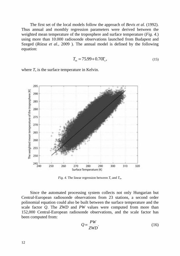
The first set of the local models follow the approach of Bevis et al. (1992). Thus annual and monthly regression parameters were derived between the weighted mean temperature of the troposphere and surface temperature (Fig. 4.) using more than 10.000 radiosonde observations launched from Budapest and Szeged (Rózsa et al., 2009 ). The annual model is defined by the following equation:

,70.099.75 sm TT += (15) where Ts is the surface temperature in Kelvin.

Fig. 4. The linear regression between Ts and Tm.

Since the automated processing system collects not only Hungarian but

Central-European radiosonde observations from 23 stations, a second order polinomial equation could also be built between the surface temperature and the scale factor Q. The ZWD and PW values were computed from more than 152,000 Central-European radiosonde observations, and the scale factor has been computed from:

.

ZWDPWQ = (16)

13

Finally, a second order polinomial was fit to the dataset of the surface temperature and the scale factor (Fig. 5):

( ) ( )2210

1)(TTaTTaa

TQSS

s −+−+= , (16)

where a0= 6.39 ± 0.0003,

a1= –1.75×10–2 ± 2.7×10–5 (1/K), a2= 7.5×10–5 ± 2.5×10–6 (1/K2) and T = 283.17 (K).

It must be noted that the polinomial coefficients a0 and a1 are quite

similiar to the original Emardson-Derks model, however the coefficient a2 has a different sign.

Fig. 5. 2nd order polinomial fit of the ratio between the ZWD and PW with respect to the surface temperature.

In order to compare the original Emardson-Derks model with the one fitted to the Central-European observations, the Q factors were computed from the surface temperatures. Afterwards, these values were compared with the factors computed from the radiosonde observations. The statistical properties of the residuals can be found in Table 2.

14

Table 2. The statistics of the residual of the scale factor (1/Q)

Minimum Maximum Mean Standard deviation

Emardson-Derks –0.344 0.289 0.061 0.092 2nd order fitted –0.277 0.277 0.000 0.092

4.2.1. Comparison of the direct and indirect approaches

The scale factor Q can be computed based on the aforementioned direct approach using the surface temperature, and using an indirect approach proposed by Bevis et al. (1992), too. In the indirect approach, the weighted mean temperature of the troposphere is computed from the observed surface temperature based on a linear regression model, and the scale factor is computed by Eq. (9).

The efficiency of the direct and indirect approaches has been compared. The scale factor Q has been computed according to both of the approaches and the values were compared with the reference values stemming from the radiosonde observations. The results (Table 3) show that the indirect approach causes a systematic bias in the computation of the Q factor in the order of 0.3%, which would lead to a similar systematic bias in the PW estimations. Although the indirect approach is more popular in the international practice, the direct approach provides slightly better results. It must also be noted, that the second order polinomial model fitted to the observed values with the standard deviation of approximately 1.5%.

Table 3. The statistics of the residual of the scale factor (1/Q) computed by the direct and indirect approaches

Minimum Maximum Mean Standard deviation

Q(Tm) –0.311 0.317 –0.020 0.092 Q(Ts) –0.277 0.277 0.000 0.092

5. Results

The automated processing system has been collecting and processesing the GNSS observations since April 14, 2011. In order to validate the results, the precipitable water vapor estimates were compared to radiosonde observations and the PW estimates stemming from ECMWF analysis. Although PW estimates

15

are available in 86 stations over Central Europe, comparisons could have been made at the 23 radiosonde sites. The results obtained in Budapest can be seen in Fig. 6, while the statistical properties can be found in Table 4. The residuals show that the ECMWF slightly underestimates the precipitable water vapor, while the GNSS overestimates it.

Fig. 6. Comparison of GNSS-derived PW with ECMWF analysis and radiosonde observations in Budapest (April 14 – May 31, 2011).

Table 4. Statistics of the fit between the precipitable water vapor from radiosonde and ECMWF analysis/GNSS estimations

Minimum [mm]

Maximum [mm]

Mean [mm]

Standard deviation [mm]

PW(Sonde) –PW(ECMWF) –4.6 4.7 0.4 ± 1.6

PW(Sonde) –PW(GNSS) –4.5 4.1 –1.2 ± 1.3

Fig. 6 shows that in some intervals the PW estimates derived from the

GNSS observations (grey continuous line) do not fit nicely to the radiosonde

0

5

10

15

20

25

30

35

Apr

il 14

Apr

il 21

Apr

il 28

May

5

May

12

May

19

May

26

[mm

]

PW (Sonde) PW (ECMWF) PW (GNSS) Precipitation

16

observations (black continuous line). This is the case for the periods April 25 – April 26, April 29 – May 1, May 21 – May 22, and for May 28. In order to find the reason for this misfit, the radar images obtained during the study period were checked and a simple function was created, which reflects the intensity of precipitation in the vicinity of the radiosonde station. The dashed black line at the bottom of Fig. 6 shows this function. Zero values mean no significant precipitation in the vicinity of Budapest, while the value of 1 denotes significant precipitation seen on the radar images. Despite this categorization is rather simple, the majority of misfits coincide with the periods, where significant precipitation could be observed. In these cases the GNSS derived PW values overestimate the precipitable water vapor with respect to the radiosonde observations.

Comparing the hourly PW estimates from GPS with the radiosonde observations, altogether 59 PW estimate residuals can be computed in the study period. Out of these, 19 had a higher absolute value than 2 mm, and in 15 cases significant precipitation could be observed on the radar images, which also show the relationship between the performance of PW estimates and the stability of the PW values around the GNSS station.

In order to find the reason for this deviation, various parameters, such as the zenith hydrostatic delay, zenith wet delay, and 1/Q factor have been compared with their counterparts computed from the radiosonde observations. The results can be seen in Fig 7, Fig 8 and Fig 9 respectively. Fig. 9 clearly shows that the estimation of the 1/Q factor does not cause large discrepancies in the PW estimates. The absolute values of the residuals are smaller than 0.2, which corresponds to the maximal error of 3% (approximately 0.6 mm) in the PW values.

The estimation of the zenith hydrostatic delays is not a key issue either. The maximal residual reached the level of – 4 mm, which corresponds to approximately 0.6 mm in the PW values. However a systematic bias can clearly be seen in Fig. 7, which needs further investigations.

The large discrepancies in the estimated PW values are most probably caused by the estimation of the zenith wet delays. Since zenith wet delays are estimated in the GNSS processing, the troposphere mapping functions need further investigations to improve the quality of ZWD estimates. Fig. 8 shows that the ZWD residuals vary in time with an order of magnitude larger amplitudes than the ZHD, reaching the level of 30 mm. This corresponds to 4.5 mm in terms of precipitable water vapor.

Since the estimation of the zenith wet delays is done using isotropic mapping functions, these estimates are likely to be less accurate when the precipitable water vapor content varies greatly in the vicinity of the GNSS stations. Thus the estimated PW values can be interpreted as mean PW values for an area with the radius of approximately 60 km.

17

Fig.7. Residuals of the ZHD values computed from the Saastamoinen model.

Fig. 8. Residuals of the ZWD values estimated from GNSS observations.

-5

-4

-3

-2

-1

0

1

2

Apr

il 14

Apr

il 21

Apr

il 28

May

5

May

12

May

19

May

26

ZHD

[mm

]

-60

-50

-40

-30

-20

-10

0

10

20

30

Apr

il 14

Apr

il 21

Apr

il 28

May

5

May

12

May

19

May

26

ZWD

[mm

]

ZWD Residual Precipitation

18

Fig. 9. Residuals of the 1/Q factor estimated from the surface temperature.

6. Conclusions and outlook

Our investigations showed that the estimation of precipitable water vapor is possible using the Hungarian Active GNSS Network (GNSSNet.hu). The near real-time processing system has been developed to process the GNSS data and collect the meteorological data sets for the estimation and validation of the precipitable water vapor.

Various mathematical models have been studied, too. A new polynomial model of the scale factor Q has been determined, which fits slightly better to the Central Europen radiosonde observations than the original Emardson-Derks model. Moreover, numerical studies prove that the direct computation of the Q factor is better than the indirect approach proposed by Bevis et al. (1992).

The results of the PW estimations agreed with the radiosonde observations at the level of ±1.3 mm in terms of standard deviation. However, large discrepancies have been found, when precipitation was observed in the vicinity of the GNSS stations. A reason for this could be the application of isotropic mapping functions, therefore, the application of advanced mapping functions should be investigated in the future.

The estimated PW values showed a systematic bias of 1.2 mm compared to the radiosonde observations. This systematic bias is most likely caused by

-0.25

-0.20

-0.15

-0.10

-0.05

0.00

0.05

0.10

0.15

0.20

0.25

Apr

il 14

Apr

il 21

Apr

il 28

May

5

May

12

May

19

May

26

1/Q

19

seasonal effects in the GNSS coordinates, which were neglected in this processing. Therefore, further adjustments in the GNSS processing strategy must be made to minimize the effect of these seasonal coordinate variations on the precipitable water vapor estimates. Acknowledgements—The authors would like to thank the financial support of the Hungarian Research Fund (OTKA) in the frame of the project K-83909. This work has been done in the frame of the „Development of quality-oriented and harmonized R+D+I strategy and functional model at BME" project. This project is supported by the New Hungary Development Plan (Project ID: TÁMOP-4.2.1/B-09/1/KMR-2010-0002). The authors would also like to thank the funding of the European Union and the co-financing of the European Social Fund in the frame of the project TÁMOP 4.2.1./B-09/1/KMR-2010-0003. Special thanks for István Ihász (Hungarian Weather Service) for preparation of ECMWF precipitable water vapor dataset.

References

Ádám, J., Bányai, L., Borza, T., Busics, Gy., Kenyeres, A., Krauter, A., Takács, B., 2004: Satellite

positioning (in Hungarian). Műegyetemi Kiadó, Budapest, 458. Bányai L., 2008: The application of Global Positioning System in Earth Sciences (in Hungarian).

Geomatikai Közlemények XI, Sopron, 1–181. Bevis, M., Businger, S., Herring, T.A., Rocken, C., Anthes, A., Ware, R., 1992: GPS meteorology:

Remote sensing of atmospheric water vapor using the global positioning system. J. Geophys. Res. 97, 15 787–15 801.

Bi, Y., Mao, J., Li, C., 2006: Preliminary results of 4-D water vapour tomography in the troposphere using GPS. Adv. Atmos. Sci. 23, 551–560.

Borbás, É, 2000: A new source of meteorological observations: the Global Positioning System. PhD thesis, Loránd Eötvös University, Budapest.

Bosy, J., Rohm, W., Sierny, J., 2010: The concept of near real time atmpshere model based on the GNSS and meteorological data from the ASG-EUPOS reference stations. Acta Geodyn. Geomater. 7, 253–263.

Braun, J., Rocken, C., Ware, R., 2001: Validation of line-of-sight water vapour measurements with GPS. Radio Sci. 36, 459–472.

Dach, R, Hugentobler, U., Fridez, P., Meindl, M., 2007: Bernese GPS Software, Version 5.0. Astronomical Institute, University of Bern.

Emardson, T.R., Derks, H.J.P., 2000: On the relation between the wet delay and the integrated precipitable water vapour in the European atmosphere. Meteorol. Appl. 7, 61–68.

Hoffmann-Wellenhof, B., Lichtenegger, H., Wasle, E., 2008: GNSS – Global Navigation Satellite Systems. Springer Verlag, 516.

Hopfield, H.S., 1969: Two-quartic tropospheric refractivity profile for correcting satellite data. J. Gephys. Res. 74, 4487–4499.

Igondova, M., Cibulka, D., 2010: Precipitable Water Vapour and Zenith Total Delay time series and models over Slovakia and vicinity. Contrib. Geophys. Geod. 40, 299–312.

Karabatic, A., Weber, R., Haiden, T., 2011: Near real-time estimation of tropospheric water vapour content from ground based GNSS data and its potential contribution to weather now-casting in Austria. Adv. Space. Res. 47, 1691–1703.

Li, Z., Muller, J.-P., Cross, P., 2003: Comparison of precipitable water vapor derived from radiosonde, GPS and Moderate Resolution Imaging Spectroradiometer measurements. J. Geophys. Res. 1008(D20), 4651.

Moore, A.W., Neilan, R.E., 2005: The International GPS Service tracking network: Enabling diverse

20

studies and projects through international cooperation. J. Geodyn. 40, 461–469. Niell, A.E., 1996: Global mapping functions for the atmosphere delay at radio wavelengths. J.

Geophys. Res. 101(B2), 3227–3246. Niell, A.E., Coster, A.J., Solheim, F.S., Mendes, V.B., Toor, P.C., Langley, R.B., Upham, C.A., 2001:

Comparison of Measurements of Atmospheric Wet Delay by Radiosonde, Water Vapor Radiometer, GPS and VLBI. J. Atmos. Ocean Tech. 18, 830–850.

Plag, H.-P., Pearlman, M. (eds.), 2009: The Global Geodetic Observing System: Meeting the Requirements of a Global Society on a Changing Planet in 2020. Springer, Doldrecht Heidelberg, London, New York, 325.

Reigber, C., Lühr, H., Schwintzer, P., Wickert, J., 2005: Observations with CHAMP. Results from Three Years in Orbit. Springer Verlag Berlin-Heidelberg-New York, 630.

Rothacher, M., Beutler, G., 1998:The role of GPS in the study of global change. Phys. Chem. Earth 23, 1029–1040.

Rózsa, Sz., Dombai, F., Németh, P., Ablonczy, D., 2009: The estimation of integrated water vapor from GPS observations. Geom. Közl., XII(1), 187–196.

Rózsa, Sz., Kenyeres, A., Weidinger, T., Gyöngyösi, A.Z., 2010: The near realtime processing of GNSS observations for meteorological applications. Geom. Közl., XIII(2), 55–65.

Saastamoinen, J., 1972a: Contributions to the theory of atmospheric refraction. B. Géodes. 105, 279–298. Saastamoinen, J., 1972b: Contributions to the theory of atmospheric refraction. B. Géodes. 105, 383–397. Thayer, G. D., 1974: An improved equation for the radio refractive index of air. Radio Sci. 9, 803–807. Yahya, M. H., Kamarudin, M.N., Lim, S., Rizos, C. 2008: The potential of Global Positioning System

in weather and environmental studies. 9th SENVAR & 2nd ISESEE 2008 Conference, Shah Alam, Malaysia, 1–3 December, 527–534.

21

IDŐJÁRÁS Quarterly Journal of the Hungarian Meteorological Service

Vol. 116, No. 1, January–March 2012, pp. 21-38

Remote sensing for natural hazard mitigation and climate change impact assessment

Zsófia Kugler

Department of Photogrammetry and Geoinformatics Budapest University of Technology and Economics

Műegyetem rkp. 3, H-1111 Budapest, Hungary E-mail: zsofia.kugler@mail.bme.hu

(Manuscript received in final form December 16, 2011)

Abstract—Geographic data and remote sensing have become sophisticated tools for obtaining knowledge on natural hazards of meteorological origin. In many cases the impact of disasters can not be prevented, however, efficient mitigation strategy and rapid response can reduce losses and damages in emergency situations. In addition, climate change is expected to increase the magnitude and frequency of natural hazards like extreme precipitation, floods, hurricanes, droughts. This paper aims at demonstrating the potential of satellite image analysis and Geographic Information Systems (GIS) for assisting disaster management before and during catastrophic events. Furthermore, it describes application of remote sensing to support climate change impact assessment on hydrological cycle in sensitive arctic regions. Divers applications in Hungary and around the world will illustrate the capabilities of the technology. Operational and scientific advantages of the practice will justify the use of geographical data in managing natural hazards with origin in meteorology. Not only for analyzing the hazard with an element at risk method but also for estimating the vulnerability factor accounting for physical and socio-economic resilience of the affected area.

Key-words: natural hazards, satellite imagery, GIS, flood mapping, flood detection, arctic

region, climate change impact, river ice break-up

1. Introduction

The rapid economical and social development of our ages appears to increase the number of total deaths caused by natural disasters of meteorological origin. Hydrological hazards are causing 40% of the damages globally each year. Although some catastrophes can not be avoided, the social-economic impact of natural risk may be reduced by enhancing the effectiveness of disaster management. The security of the residents on floodplains is highly determined

22

by finding the appropriate mitigation approach to reduce vulnerability. The state-of-the-art technology of remote sensing and Geographic Information Systems (GIS) can respond to this need by delivering accurate spatial information before, during, and after the disaster (Kovács, 2010).

During a natural disaster of meteorological origin, great amount of spatial information need rises. Where did the disaster strike? What is the extent of the disaster, what is the magnitude of the event? Who was affected? Where and how to execute emergency operations? Where to set up evacuation shelters? Traditionally, all these questions may be answered by extracting information from analogue printed maps. However, the state-of-the-art technology of GIS and remote sensing can respond more sophistically to this spatial information need. For this reason during the last decade, several Earth observation satellite sensors were launched with the specific aim to assist disaster management and hazard awareness. Not only to improve knowledge of the flood hazard before the disaster happens but also to assist disaster response when the disaster strikes.

A great number of advantages are related to the use of satellite imagery in disaster management:

• far, inaccessible areas can be monitored without the need of field observations;

• images can be acquired with high revisit frequency – in specific cases almost in near real-time;

• data can be obtained large-scale with a unique observation method.

All these advantages facilitate the technology to play a significant contribution in fulfilling the geographic information need of hazard assessment and disaster management. Remote sensing not only plays a role after the disaster strikes, but assists research to reduce the negative effect of flood hazard in a pre-disaster situation too.

In this paper, first, an application will be described in details assisting flood disaster response. Then the use of satellite technology for flood hazard mitigation and climate change impact assessment will be discussed.

2. Flood disaster response with satellite imagery and GIS

The use of remote sensing tools for flood disaster mapping dates back to the early years of the first optical satellite systems like the Multi-Spectral Scanner (MMS) in the 1970` and 1980`. With the technical development of our age, several satellite systems were put on orbit lately with the aim to assist not only Earth observation but, especially, to obtain information during crisis situations. The Moderate Resolution Imaging Spectroradiometer (MODIS), a low

23

resolution (250 m) NASA satellite is playing a key contribution in disaster applications. The two platforms carrying MODIS sensor on board the Aqua (launched in 2002) and Terra (launched in 1999) platforms are monitoring the Earth every day with an almost full coverage of its complete surface. It has the significant potential to enable observing and updating information on crisis situations every day. Data can be obtained on no charge basis. Furthermore, near real-time data is available some hours after acquisition, which can assist rapid response to crisis situations. Orbital swath images are available approximately 2.5 hours after observation from NASA’s LANCE data centre (LANCE, 2011).

For all the above advantages, MODIS is playing a unique contribution to map natural disasters, especially to monitor the evolution of floodplain flooding from day to day. Therefore, numerous applications have flourished in the past using MODIS images to assist disaster mapping (Zhan et al., 2002; Thenkabail et al., 2005; Sakamoto et al., 2007). One of the major contributors of flood mapping is the Dartmouth Flood Observatory (Brakenridge et al., 2005). A global flood atlas has been developed at DFO for major floods from 2000 to recent based on optical MODIS imagery.

During the large-scale inundation in Southern Africa at the beginning of the year 2001, flood mapping was carried out with the assistance of the author at the German Aerospace Center (DLR) too. Heavy long lasting rainy season starting in early January lasting several months was causing above normal flood peaks in the River Zambezi in Mozambique. The serious flood disaster was leading to over 100 deaths and 90 000 displaced people in the river basin. Information on flood hazard from satellite sensors was combined with spatial data on vulnerability. Resulting maps could assess the magnitude of damages and losses in the disaster. Consequently, they could help to reduce uncertainties in problem solving and improve decision making for stakeholders involved in the emergency response.

The assessment of the crisis situation in the Zambezi valley is a good example of how spatially related information combined with satellite images and digital maps can help in emergency situations. MODIS imagery was used to obtain information on the inundation extent (Fig. 1). After acquiring satellite data, geometric distortion was corrected using orbital reference data. Classification of inundated areas was carried out using the 250 m highest resolution spectral band of the visible red (0.620 – 0.670 μm) and the near-IR (0.841– 0.876 μm) channels. According to the spectral reflectance characteristics of water surfaces, the two bands were suitable for classifying water bodies. From several multispectral image transformation methods, best results were obtained when using a simple arithmetic subtraction of the two available bands as follows:

NIRRFloodmask −= . (1)

24

Near-IR was subtracted from red band, where resulting images showed an enhanced contrast between land and water. Finally, a threshold value has been set up on empirical basis to divide water from land. The only feature type of the image that had unfortunately the same spectral characteristic and could not be divided from water, was cloud shadow. Flood maps were derived for the Zambezi River valley in Mozambique resulting in more 12 000 km2 of area under water cover (Fig. 1).

In a next step, spatial analysis was performed in GIS environment combining the flood extent maps and spatial data on administrative entities plus the number of inhabitants. As a result information on the effected inhabitants could be extracted. In the example showed in lower Fig. 1, the number of affected inhabitants was weighted by the proportion of flooded and non-flooded area in each administrative entity. As a result, seriously hit regions could be revealed, like the province at the confluence of the Shire and Zambezi rivers, where large lakes were formed between the two rivers.

Fig. 1. Flood mapping from MODIS images along the River Zambezi in Mozambique, 2001, and the spatial analysis of the disaster situation by GIS. (Kugler, 2004/1)

25

Beyond obtaining data, the dissemination of the acquired information is crucial in disaster situations. In many cases Internet is used to target end-users. Interactive Web GIS systems – similarly to GoogleMap – can serve not only as a platform of data exchange, but as a possibility to visualize and transmit geographic data for a world-wide audience. For the demonstrated application in Mozambique, a Web GIS system of the freeware UMN MapServer was developed as one possibility to disseminate and publish geographic information about the flood crisis through the World Wide Web.

Further to this, a mobile GIS application was developed as a source of interactive spatial data on-site, for the case when communication with an online server storing the spatial database is interfered or completely cut (Fig. 2). It stores its own spatial database locally at the client’s side, thus, the system does not have to connect trough the Internet to the central database – like the Web GIS applications described above – in order to display geographic information at the client’s side. However, a central database is still a substantial part of the system, since it may serve as a platform of data exchange between the client and the central data server. Moreover, updates of geographic data captured by clients working on-site may be uploaded to the central database. Then spatial data can be downloaded to online. Consequently, the exchange of updated information can be carried out through the central database communicating both with mobile clients and Web GIS systems. The developed system was assisting flood mitigation efforts in Mozambique, yet it can be implemented to any further region.

Fig. 2. Architecture of mobile mapping system connected to a central database for on-site disaster data acquisition and update. (Kugler, 2004/2) In lack of spatial data to support risk modeling and calculation of

meteorological hazards, historical maps of past events can be processed too. The combination of satellite based information and GIS can not only provide updates

Database DLR

(E:35°, S:9°)

GPS

26

on current disaster situations but is also able to handle historical data about past events to assess their former impact. This allows a better understanding of natural hazards and their possible future impact based on historical events.

An example of that was the detailed analysis of the well documented great flood in 1838 in Budapest, Hungary, where the River Danube flooded almost 80% of the city in March. Historical maps recorded the extent of the flood event, from which spatial information could be collected. Historical maps were acquired by the crisis management team of the Department of Photogrammetry and Geoinformatics at the Budapest University of Technology and Economics. After a geometrical transformation of the map, inundation extent was collected and combined with current maps in a GIS environment (Fig. 3).

Historical flood extent shows that only a minor part of the city centre was saved on the Pest side, while the Buda side was affected less. The reason for that is obvious when further combining the flood extent data with topographic information. The Pest side of the riverbank is flat, the Buda side is more hilly.

The acquisition of spatial information on historical disaster events can help to obtain a primarily assessment of possible future impact.

Fig. 3. Virtual view of the great flood in 1838 along the River Danube in Budapest from historical maps (left). Historical map combined with current maps shows structural changes of the channel geometry after the great flood (right). (Ládai et al., 2004)

3. Satellite detection of flood events

Remote sensing and GIS can contribute to the mitigation of emergency situations as discussed in the previous chapters. Furthermore, the technology also enables to provide early detection of major flood disasters. Generally, emergency alerting relies on national or global network of in-situ river gauging measures or on international media reports of disaster events. However, in lack of in-situ measurements, satellite data can play a key contribution in detecting major flood disasters around the globe. To fill this lack, a space-borne methodology was developed using AMSR-E passive microwave data providing near real-time, systematic detection of river floods around the world.

27

Observing hydrological conditions of river reaches from space dates back to the earlier decades. The use of optical sensors in the visible or infrared portion of the spectrum introduced in the previous chapters can be limited due to cloud cover. Thus, the systematic tracking of river reaches is not feasible in constant time intervals. To overcome this, active satellite systems, penetrating cloud cover, were used for monitoring river hydrology. Besides inundation area delineation (Hess et al., 1995), radar altimetry was applied in different studies to measure stage elevation or water surface level change directly (Brikett, 1998; Koblinsky et al., 1993). The renowned scientific study of Alsdorf et al. (2000) describes water level measurement based on interferometic radar data acquired by the SRTM mission over the Amazon basin. Still, the mentioned NASA topographic mission was providing observations only over a short time period, thus the technology could not be implemented on an operational basis.

Other studies were using passive microwave emission of the Earth’s surface to estimate flooded area from space. The first pioneer study of using passive microwave sensors to estimate inundated area was set up by Stippel et al. (1994) in the Amazon basin using the Scanning Multichannel Microwave Radiometer (SMMR). The NASA sensor was providing measurements from 1978 to 1987 and has been used to measure time series of water levels on very large rivers, such as the Amazon. Nevertheless, the measurements of the SMMR instrument were only available in weekly intervals.

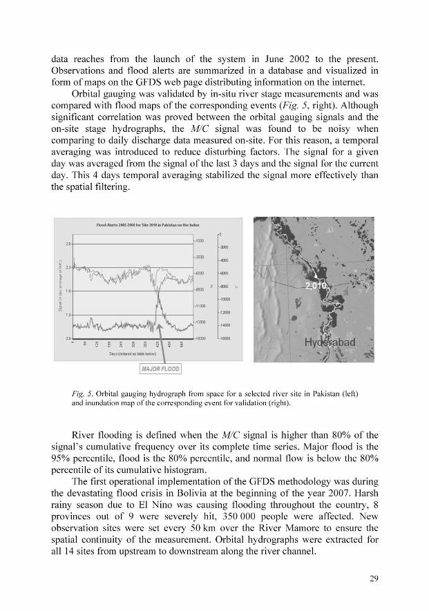
Yet, all these applications did not support operational daily observations of river gauging in near real-time with global coverage. For this reason, a system has been developed to monitor river conditions using passive microwave observations of Advanced Microwave Scanning Radiometer (AMSR-E). The system set-up at the Joint Research Center with the assistance of the author (Kugler et al., 2007) is based on the methodology developed by Brakenridge et al. (2007) at the Dartmouth Flood Observatory. The aim of the Global Flood Detection System (GFDS) is to monitor river sites and detect flooding by using the radiation difference of land and water on passive microwave images. The operational system is acquiring, updating, and providing data every day on a global scale not restricted by cloud cover. With current fast internet technologies data is delivered to the users in less than half a day after the acquisition (http://www.gdacs.org/flooddetection/).

The technique uses AMSR-E microwave remote sensing data of the descending orbit, H polarization, 36 GHz frequency band which is sensitive to water surface changes. Brightness temperature measured by the sensor onboard is related to the physical temperature (T ) and the emissivity (ε ) of an object:

.TTb ε= (2) Due to the different thermal inertia and emission properties of land and

water, the observed microwave radiation, in general, accounts for a lower

31

in flood disasters. Yet microwave data has the significant advantage of not being hindered by cloud cover during the event.

Fig. 7. Orbital gauging measurements in time and space along the Mamore River in Bolivia during the great flood event of 2007. Flood wave propagation is remarkably visible from 3D graph both in time and space. (Kugler, 2007).

4. Effects of global climate change on arctic river hydrology

Orbital GFDS technology allows not only the monitoring of flood events but also observing other changes in hydrological conditions. Using the GFDS methodology, river ice freezing and melting can be monitored in arctic regions without the need of in-situ measurements. The extent of polar sea ice cover and ice shield is a well-known indicator of global climate change. Satellite observations have been used for long time to operationally monitor sea ice cover and its changes in the past decades (Maslanik et al., 1999; Cavalieri et. al., 2003; Rodrigues et al., 2008; and Kwok et al, 2009). Yet no regular observations are carried out on continental arctic rivers, even though their annual spring ice break-up and freezing would also serve as a notable sign for climate change processes. The lack of traditional hydrological measurements in those remote inaccessible regions makes the use of satellite data a key technique in obtaining information on their hydrological cycle. The analysis of arctic regions can contribute to the quantitative and qualitative estimations of the global impact.

For this reason, satellite data was used to estimate spatial and temporal patterns of arctic river ice from satellite sources like MODIS and AVHRR

33

The aim was to reveal possible effects of global climate change on arctic rivers. Anomalies in the period of seasonal river ice melting in spring were analyzed in detail. Orbital gauging observations were set every 50 km in the selected large river valleys to obtain high spatial resolution of the analyses.

The selected rivers generally run from south to north crossing different climate zones. For this reason, melting in spring starts in the lower latitudes and propagates downstream to the north with time. Further to this, there is a strong drift of climatic origin from the most west river of Ob starting to melt at the begin of May to the most east river of Kolyma, where ice break-up starts only at the end of May.

A pilot study has been carried out to extend AMSR-E time series with Special Sensor Microwave/Imager (SSM/I) passive microwave satellite data. Both sensors have similar properties, and images are free of charge. Likewise AMSR-E data M/C signal was extracted from 37 GHz, H polarization band of the SSM/I sensor. During the SSM/I mission, several sensors were launched into orbit starting from F8 series in 1987 to F11, 13, 17 satellite missions acquiring data till present. Based on their images, ice melting time series from AMSR-E data was extended with 14 additional years. M/C signal was obtained for selected river sites, and orbital gauging was used to detect changes during the investigated years reaching from 1989 to 2010.

To detect the timing of the ice break-up at a given river site, statistical parameters of its complete time series were calculated and defined as magnitude:

( )( )s.dev.dtans

C/WmeanC/MMagnitude −= . (5)

As a result, the M / C signal was normalized to a value that enables

comparison of different sites in various river valleys. Magnitude was below 0 during the winter freezing period and increased to above 0 when spring ice break-up started.

To assess preliminary performance of the techniques, 5 orbital gauging sites were selected and analyzed in detail for the River Lena. Sites were located 1–200 km apart from each other along the river. The day of the ice break-up was extracted and plotted for each studied year demonstrated in Fig. 9. Applying a simple linear regression model, lines were fitted to the timing curves to give a preliminary assessment of the changes in the last two decades. Estimations revealed a negative shift over the investigated gauging sites, thus, river ice appeared to break earlier with time. In average, sites were having from –2 to – 6 days changes/decade in the timing of their ice-breaking during the past two decades.

34

Fig. 9. Ice break-up extracted from orbital gauging measurements from 1989 to 2010 in selected sites along the subarctic River Lena.

Besides the River Kolyma, 4 additional arctic rivers the Ob, Yenisey, Lena in Siberia and the Machenzie in North-America were put under similar investigation. Ice break-up was extracted using the magnitude of the signal (Eq. (5)). Relationship between the day of the ice break-up and the different years was estimated using linear regression approach described above. From 50 to 80 orbital gauging sites were investigated per river valley depending on the length of the reach. The slope of the linear regression line was calculated for each site along the river. The histogram of the slopes for each river is illustrated in Fig. 10.

The peak of the distribution lays in negative values meaning that the linear regression lines have a negative direction for the majority of the investigated sites. Thus, the majority of the river sites show a change towards earlier ice break-up in time. The quantitative estimation of the trends may have unexpected uncertainties, but the direction of the changes shows similar trends in the majority of the investigated arctic river valleys.

y = -0.4754x + 139.83R² = 0.1811

y = -0.3416x + 156.97R² = 0.1418

y = -0.3298x + 140.97R² = 0.2106

y = -0.2219x + 140.42R² = 0.0514

y = -0.6714x + 142.04R² = 0.377

Apr 27

May 4

May 11

May 18

May 25

Jun 1

Jun 8

Jun 15

1989 1991 1993 1995 1997 1999 2001 2003 2005 2007 2009

83 304 1752 305 312

Lineáris (83) Lineáris (304) Lineáris (1752) Lineáris (305) Lineáris (312)

36

Fig. 11. (70°41`N

This phazardmappinobtainialso prfrom squantit

Smany even ioperatiaffect considcontinureasonopticalresolutdemonopticalconsid

Gof natu

In-situ gaugN 127°24`E)

aper demod assessmng, and ining informroved to

space. Furtative influelecting thfactors. Tif sensors ional dailyso that

dered. Actiuous mons the GFDl systems.tion of panstrated gol and mic

dering theirGlobal clim

ural hazar

ging measur, Siberia. Re

onstrated ent. Sateln lack of

mation on be suitab

rther to invuence of che most a

The major have app

y, global opassive aive system

nitoring ofDS system. Since thassive micood resultcrowave sr above m

mate changrds. The

rement of icegression ana

5.

the operatllite resouf available

risk and le for opevestigatin

climate chappropriate

limitationpropriate observatioand activms have nf flood ev

m using pahe emittedcrowave ts even insensors h

mentioned ge is expeinfluence

e break-up aalysis shows

5. Conclus

tional use urces were data, hipossible

erational ng the poshange was e sensor fn of opticresolution

ons. Cloude microwno daily gents is nossive micr

d energy fsystems in sub-pixehave greatlimitation

ected to incof the g

along the Rinegative tren

sions

of satellitre demonistorical mfuture scedaily obssible impastudied in

for hazard cal satellitn and revd cover plawave sateglobal covot feasible rowave dafrom the sis coarse. el dimenst importa

ns. crease the

global cha

iver Lena atnd. (Vuglinsk

te technolstrated fo

maps wereenarios. Servation oact of natun arctic reg

mapping te systemsvisit capabays a signllite sens

verage, foron a dail

ata is a gosurface is Still, GF

sion. For nce in ha

e magnitudange can

t Kusur statiky, 2000).

logy and Gor flood de introducatellite daof river gural hazargions. is depend

s is cloudbility to s

nificant hinsors have r this reasly basis. Food alterna

low, the FDS applithis reasoazard mit

de and frebe measu

ion

GIS for disaster ced for ata was gauging rds, the

ding on d cover, support ndering

to be son the For this ative to spatial

ications on both tigation

quency ured on

37

sensitive areas such as polar and subpolar regions. For this reason, the paper also discussed the results from the study analyzing changes in the seasonal ice break-up along arctic rivers. Results concluded an anomaly towards earlier ice melting in the majority of the analyzed river sections in Siberia and Northern America. Even though the quantitative output of the anomalies may have high standard deviation and unexpected inaccuracies, the direction of the change was found to be the same over all investigated river sites. Acknowledgement—Part of the work presented was supported by Magyary Zoltán Postdoctoral Fellowship, Budapest with the grant of the EEA and the Norwegian Financial Mechanism, and by the TÁMOP-4.2.1/B-09/1/KMR-2010-0002 Project was partly supported by the EU.

References

Alsdorf, D.E., Melack, J.M., Dunne, T., Mertes, L.A.K., Hess, L.L., Smith, L.C., 2000: Interferometric radar measurements of water level changes on the Amazon floodplain. Nature 404, 174–177.

Birkett, C.M., 1998: Contribution of the TOPEX NASA radar altimeter to the global monitoring of large rivers and wetlands. Water Resour. Res. 34, 1223–1239.

Brakenridge, G.R., Anderson, E., 2005: MODIS-based flood detection, mapping, and measurement: the potential for operational hydrological applications. In Transboundary Floods, reducing risks through flood management NATO Science Series (eds.: J. Marselek, G. Stacnalie, G. Bálint): IV Earth and Environmental Scineces 72, Springer, The Netherlands, 1–12.

Brakenridge, G.R., Nghiem, S.V., Anderson, E., Mic, R., 2007: Orbital microwave measurement of river discharge and ice status. Water Resour. Res. 43, W04405, 16 pp., doi:10.1029/2006WR005238

Cavalieri, D.J., Parkinson, C.L., Vinnikov, K.Y., 2003: 30–year satellite record reveals contrasting Arctic and Antarctic decadal sea ice variability. Geophys. Res. Lett. 30(18), 4 pp., doi:10.1029/2003GL018031.

Hess, L.L., Melack, J.M., Filoso, S., Wang, Y., 1995: Delineation of inundated area and vegetation along the Amazon floodplain with SIR-C synthetic aperture radar. IEEE Trans. Geosci. Remote Sens. 33, 896–904.

Koblinsky, C.J., Clarke, R.T., Brenner, A.C., Frey, H., 1993: Measurement of river level variations with satellite altimetry. Water Resour.Res. 29(6), 1839–1848.

Kovács, K.I., 2010: Spatial information systems for emission reduction. Clean Technol. Environ Policy 12, 647–651.

Kugler, Zs., 2004/1: The Use of GIS and Remote Sensing in Flood Disaster Management in Mozambique. In: II. PhD CivilExpo Symposium Proceedings: BUTE Dept. of Highway and Railway Engineering (eds.: Barna Zs., Fenyős D.), Budapest, Hungary, 84–88., ISBN: 963-421-600-5.

Kugler, Zs., 2004/2: A 2001. évi mozambiki árvízkatasztrófa felmérése és koordinálása a távérzékelés és térinformatika segítségével. Geometriai Közlemények VII, 139–148.

Kugler, Zs., De Groeve, T., Brakenridge, G.R., Anderson, E., 2007: Towards Near real-time Global Flood Detection System. Int. Arch. Photogramm. Rem. S. XXXVI:(PART 7/C50), 1–8.

Kwok, R., Rothrock, D.A., 2009: Decline in Arctic sea ice thickness from submarine and ICESat records: 1958-2008. Geophys. Res. Lett. 36, L15501.

Ládai, A.D., Kugler, Zs., Tóth, Z., Barsi, Á., 2004: A pest-budai nagy árvíz térinformatikus szemmel. Térinformatika XVI (7), 16–18.

LANCE (Land Atmosphere Near Real-time Capability for EOS), 2011: Rapid Response system, Near Real Time (Orbit Swath) Images. [Online] available: http://lance-modis.eosdis.nasa.gov/cgi-bin/imagery/realtime.cgi, last access: 2011-09-16

Maslanik, J.A., Serreze, M.C., Agnew, T., 1999: On the record reduction in 1998 western Arctic sea-ice cover. J. Geophys. Res. 26, 1905–1908.

38

Overland, E., Wang, M. Salo S., 2008: The recent Arctic warm period. Tellus A 60, 589–597. Pavelsky, T.M., Smith, L.,C., 2004: Spatial and temporal patterns in Arctic river ice breakup observed

with MODIS and AVHRR time series, Remote Sensing of Environment, Volume: 93, 328–338. Rodrigues, J., 2008: The rapid decline of the sea ice in the Russian Arctic. Cold Reg. Sci. Technol. 54,

124–142. Sakamoto, T., Nguyen, N.V., Kotera, A., Ohno, H., Ishitsuka, N., Yokozawa, M., 2007: Detecting

temporal changes in the extent of annual flooding within the Cambodia and the Vietnamese Mekong Delta from MODIS time-series imagery. Remote Sens. Environ. 109, 295–313.

Shiklomanov, A.I., Lammers, R.B., Vörösmarty, C.J., 2002: Widespread Decline in Hydrological Monitoring. Threatens Pan-Arctic Research. EOS Transactions, American Geophysical Union 83(2), 13–17.

Sippel, S.J., Hamilton, S.K., Melack, J.M., Choudhury, B.J., 1994: Determination of inundation area in the Amazon River floodplain using SMMR 37 GHz polarization difference. Remote Sens. Environ. 48, 70–76.

Thenkabail, P.S., Schull, M., Turral, H., 2005: Ganges and Indus river basin land use/land cover (LULC) and irrigated area mapping using continuous streams of MODIS data. Remote Sens. Environ. 95, 317–341.

Vuglinsky, V., 2000: Russian river ice thickness and duration. Boulder, CO: National Snow and Ice Data Center/World Data Center for Glaciology. Digital media.

Zhan, X., Sohlberg, R.A., Townshend, J.R.G., DiMiceli, C., Carroll, M.L., Eastman, J.C., 2002: Detection of land cover change using MODIS 250 m data. Remote Sens. Environ. 83, 336–350.

39

IDŐJÁRÁS Quarterly Journal of the Hungarian Meteorological Service

Vol. 116, No. 1, January–March 2012, pp. 39–52

The effect of fertilization and precipitation on the yield of maize (Zea mays L.) in a long-term experiment

János Nagy Centre for Agricultural and Applied Economic Sciences,

University of Debrecen, Böszörményi út 138, H-4032 Debrecen, Hungary

Email: nagyjanos@agr.unideb.hu

(Manuscript received in final form February 22, 2012)

Abstract—This study examines how the amount of precipitation, the NPK fertilizer treatment and their interaction affects maize yield. The measurements were carried out at the Látókép experiment site of the University of Debrecen (Debrecen, Hungary N: 47o33’, E: 21o27’, 113−118 metres above sea level) on mid-heavy calcareous chernozem soil in a multifactoral long-term field experiment established in 1984. 17-year-long data series were used (1990–2008) in the study. We examined how the precipitation during the growing season and the winter period affected maize yield and demonstrated into that there was a strong positive correlation (r = 0.710; p < 0.01) between the amount of precipitation during the growing season and yield. Based on the effective heat units (EH) and the potential evapotranspiration (PET) values, the growing seasons of the long-term experiment were separated to dry and wet years. The difference between the average yields of dry and wet years was significant (p < 0.05). Significant difference was obtained (p < 0.05) between the non-fertilized and fertilized treatments (60 and 120 kg N ha–1). The 120 kg N ha–1 treatment did not significantly increase the maize yield in comparison with the 60 kg N ha–1 treatment. The evaluation of the joint effect of fertilization and precipitation on yield showed that fertilization is responsible for nearly twice as much of the standard deviation of yield as the amount of precipitation. In dry years, there was a significant difference only between the non-fertilized and fertilized treatments, whereas in wet years, we even found a statistical difference between fertilizer doses. As regards fertilizer treatments, higher yields were obtained in wet years than in dry ones. Altogether, statistical evaluations showed that the nutrient utilization of the applied fertilizer is determined by precipitation supply. In dry years, only smaller fertilizer doses (60 kg N ha–1) were utilized, higher doses were not necessary. In wet years, higher doses (120 kg N ha–1) induced significantly higher yield and higher extent of nutrient utilization.

Key-words: maize, precipitation, fertilization, long-term field experiment

40

1. Introduction

The high variability of climate is one of the biggest risk factors of production and agricultural producers have to continuously consider this factor. Over many years, differences in temperature and precipitation, as well as their distribution, significantly affect yield and yield quality, even in the case of very similar production technologies.

In the last century, the proportion of drought or extremely wet years significantly increased. Both have a negative effect on maize production and its predictability. Barrov et al. (2000) reached a similar conclusion when they determined the change of the quantity of precipitation in winter (0.4−3.6%) and summer ((–0.5)−3.7%) periods between 1961–1990. Láng (1976) and Márton (2002) showed the significant effect of weather on yield. Berényi (1956) established that natural water supply determined 55–75% of yield.

Water has multiple and rather complex roles in the life and metabolism of plants. The rate of growth of maize reacts in a much more sensible and much quicker way to the change of water supply than any other change in the environmental factors. Water stress during vegetative development reduces the growth of stem and leaf cells, which then leads to the decrease of crop height and leaf area (Lauer, 2003). Drought during tasselling could result in 40–50% yield loss (Claassen and Shaw, 1970). Water shortage during tasselling and flowering reduce the grain number per row, whereas water stress after pollination decreases grain weight, thereby causing a significant yield drop (Shaw, 1977; Westgate and Boyer, 1986; Lauer, 2003). Kiesselbach (1950) states that temperature and water supply have significant effects during grain filling. Drought during grain filling usually results in the development of smaller grains (Smith et al., 2004). As a result of unfavourable water supply, the speed and duration of dry matter incorporation decreases (Quattar et al., 1987). Westgate and Garnt (1989) pointed out that even a shorter period of water shortage caused a significant drop in the water content of grains.

Besides the level of water and nutrient supply, the efficiency of maize production is also determined by the date of fertilization and its distribution. Therefore, professional fertilization is the basic requirement of optimal crop production. During the determination of the optimal date of fertilization and the optimal fertilizer dose, producers have to consider the transformation, leaching and fixing processes in the soil, the nutrient absorption ability and fertilizer reaction of the produced hybrid, as well as the effect of precipitation (Hansen and Djurhuus, 1996; Delphin, 2000; Ichir et al.,2003; Nakamura et. al., 2004; Körschens, 2006).

The results of long-term fertilization field experiments provide an opportunity to evaluate multifactoral interactions in crop production and environmental protection research projects (Körschens, 2006; Nagy, 2008). The aim of this study was to examine the effect of precipitation – as an independent

41

variable – during winter and the growing season, as well as the effect of NPK fertilization on yield. Furthermore, we examined the effect of the interaction of these two factors on maize yield.

2. Materials and methods

The measurements were carried out at the Látókép experiment site of the University of Debrecen (Debrecen, Hungary N: 47o33’, E: 21o27’, 113−118 metres above sea level) in a multifactoral long-term field experiment established in 1984. 17 year long data series were used (1990–2008) in the study.

Soil properties of the field experiment: The experiment was carried out on mid-heavy calcareous chernozem soil.

Based on the soil analysis results obtained in 2008, the average pHKCl of the soil was 6.6 (slightly acidic), which is optimal from the aspect of the nutrient uptake of the crop. The physical type of the soil was mid-heavy adobe. The soil plasticity of the upper (0.2 m) layer was 39 (Arany’s number). The total soil water-soluble salt content (anions and cations) was 0.05% (low salt content soil). The calcium carbonate content in the upper 0.8 m of soil was 0% (i.e. there is a chalk deficiency), but it gradually increased between 1 m and 1.6 m, reaching 11% (i.e. moderately chalky). The organic matter of the soil was 2.4% in the upper 0.2 m of soil, whereas it did not exceed 1% at a depth of 1.2 m. The soil nitrogen and potassium supply was good and the phosphorous content was average.

Fertilizer treatments: The basic dose was 30 kg N ha–1, 23 kg P2O5 ha–1, 27 kg K2O ha–1. Fertilizer

treatments of 1, 2, 3, 4 and 5 times higher than this dose were applied and a non-fertilized treatment was also included. we examined the results of the non-fertilized treatment and the 60 kg N ha–1, 46 kg P2O5 ha–1, 54 kg K2O ha–1 (indication: 60 kg N ha–1), 120 kg N ha–1, 90 kg P2O5 ha–1, 106 kg K2O ha–1 (indication: 120 kg N ha–1) treatments. The entire quantity of fertilizers was applied in spring. The experiment had a strip plot design, with the 30 hybrid and fertilizer treatments located crosswise in four replications. The plant density was 70 thousand plants ha–1. In order to determine the nitrate N content of the soil, soil samples were taken twice a year in spring (one week before sowing) and after harvest from the 0 –200 cm soil layer.

Weather parameters: Environmental parameters at the Research Plant of the University were

continuously measured and logged by an automatic data-logging station. Air temperature (°C) at heights of 0.5, 1 and 2 m, relative humidity (%) soil

42

temperature (°C) at depths of 50, 250 and 500 mm, incoming radiation (W m–2) and the amount of precipitation (mm) were measured every sixth second. The statistical parameters derived from the data (average, standard deviation) were stored every 15 minutes. Basic data are accompanied by pheno- and phytometric observations and soil analyses. we used the following equation to calculate heat units – one of the most important criteria in maize growing – over the entire growing season (Table 1):

( )

basisminmax

n

iTTTHU −−=∑

= 2

1, (1)

where HU indicates the heat unit,

Tmax indicates maximum daily temperature,

Tmin stands for minimal daily temperature,

Tbasis indicates the base temperature for crop development, which is 10oC

in the case of maize (Davidson and Campbell, 1983; Gallagher, 1979; Nield and Seeley, 1977).

Table 1. Precipitation, effective heat sum and potential evapotranspiration (Debrecen, 1990–2008)

Years Precipitation during the growing season (mm)

Heat unit (oC)

Potential evapotranspiration (mm day–1)

1990 202 1175 625 1992 180 1531 693 1993 253 1381 665 1994 240 1461 681 1996 428 1336 655 1997 248 1424 672 1998 472 1420 671 1999 389 1537 691 2000 196 1502 687 2001 402 1380 666 2002 256 1288 650 2003 219 1439 679 2004 343 1168 624 2005 499 1302 649 2006 326 1414 670 2007 284 1573 704 2008 484 1475 680

43

There are numerous methods for the determination of potential evapotranspiration (PET), some of which are empirical correlations, others are multivariate functions calculated with statistical methods, whereas the most recently applied formulae are derived from the most important thermodynamic parameters. Among others, these are the methods of Penman (1948), Thornthwaite (1948), Mckenny and Rosenberg (1993) and Szász (1977). We used the method of Szász (1977) to determine the value of PET. This method provides a highly accurate estimation and it considers the atmospheric elements and processes significantly determining the evaporation of water – air temperature, the relative moisture content of water vapour, wind speed and microadvection effects.

( ) ( ) ( )[ ]vfRT.PET 322 12100950 −−= β , (2)

where PET is the potential evapotranspiration (mm day–1),

T is the daily mean temperature (°C), R is the degree of saturation, ƒ(ν) is the effect function of wind speed,

β is the coefficient for the expression of the oasis effect.

The oasis effect is the quotient of the environment and the evaporating water.

( )( )water

soilccρρβ = (3)

The numerator covers the heat capacity of the environment and the soil and the denominator is the heat capacity of water. The heat capacity of water is 4.19 J cm–3.

The heat capacity of wet soil: tftfv L.N..c 0012024840 ++= γ , (4)

where γ is the volume mass (g cm–3), Ntf is the moisture content (cm3

cm–3), Ltf is the air content (cm3

cm–3).

Statistical procedures: In order to examine the effect of precipitation during the winter period and

the growing season on yield, we determined the coefficient of correlation between the variables. Based on the available weather data, we separated the examined years into groups by using hierarchical cluster analysis. We used variance analysis to examine whether there is any difference between the two

44

groups as independent variables identified by the cluster analysis from the aspect of the effect on yield. We ran a Kruskal-Wallis non-parametric test generally used for the comparison of the means of three or more samples concerning the whole sample to examine the effect of fertilization on maize yield. We applied paired Mann-Whitney U test with Bonferroni correction to examine the differences between treatment means.

We analysed the common effect of dry and wet years and fertilizer treatments as independent variables on maize yield. We separately evaluated the differences between fertilizer effects in dry and wet years, as well as the effect of precipitation on different fertilizer levels. Following this, we categorized the examined years from the aspect of yield using hierarchical cluster analysis (very low, low, high, very high).

3. Results and conclusions

3.1. The effect of precipitation during the winter period and the growing season on maize yield

Based on the value of Pearson’s correlation coefficient (using a paired test), it was shown that there is a strong positive correlation between the precipitation in the growing season and yield (r = 0.718, p < 0.01) at 1% level of significance (Fig. 1), similar to the results of Aguilar et al. (2007).We could not show any correlation between the amount of precipitation in the winter period and the yield, therefore, we only analysed the correlation between the data during the growing season and yield.

600500400300200100

Precipitation during the growing season (mm)

R Sq Linear = 0,515

9 8 7 6 5 4 3

100 200 300 400 500 600 Precipitation during the growing season (mm)

R Sq Linear=0.515

Precipitation (mm)

Yie

ld (t

ha–1

)

Fig. 1. Correlation between the precipitation during the growing season and yield (Debrecen, 1990–2008).

45

In itself, the amount of precipitation does not determine the amount of water available for maize. Using the data available at the meteorological station of the university, we calculated the values of the effective temperature (ET) and potential evapotranspiration (PET) for the entire growing season (Table 1). Based on the amount of precipitation during the growing season, the ET and PET values, we used hierarchical cluster analysis to classify the years into groups. One of the groups was named dry years and the other one was named wet years. Of the 17 experimental years, the following ones were dry: 1990, 1992, 1993, 1994, 1997, 2000, 2002, 2003, 2007; wet years: 1996, 1998, 1999, 2001, 2004, 2005, 2006, 2008. (The years 1991 and 1995 were excluded from the analysis, due their extreme values and the „sensitivity” of the statistical analyses.) The average amount of precipitation in the growing season (April-September) was 231 mm in dry years and 418 mm in wet years. The potential evapotranspiration was 673 mm on average in dry years during the growing season and 626 mm in wet years.

The results of the variance analysis showed that there is a significant difference (p < 0.05) between the average maize yields of wet and dry years. The average yield was 6.96 t ha–1 in dry years and the water supplied by precipitation significantly increased maize yield (by 2.19 t ha–1). Every millimeter of precipitation in the growing season was associated with 34 kg grain yield in dry years and 45 kg in wet years.

During the 17 years of the long-term experiment, yields varied greatly from year to year. The lowest maize yield was obtained in 2007 (5.21 t ha–1), whereas the highest yield was harvested in 2008 (11.41 t ha–1) (Fig. 2 and 3).

1990 1992 1993 1994 1997 2002 2003 2007 Dry years

Yie

ld (t

ha–1

)

14

12

10

8

6

4

Fig. 2. Average yield of maize in dry years.

46

200820062005200420012000199919981996

4

2

0

8

6

4

1996 1998 1999 2000 2001 2004 2005 2006 2008 Wet years

Yie

ld (t

ha–1

) 14

12

10

8

6

4

Fig. 3. Average yield of maize in wet years.

3. 2. Evaluation of the effect of fertilization

Precipitation during the growing season greatly determines the leaching of nitrogen forms and the utilization of the nitrogen active ingredient. Only a part of the active ingredient content of the applied N fertilizer is present in the yield, the rest is leached out, it denitrificates or is transformed in other ways (Kavlen et al., 1998; Díez et al., 2008). Due to the high amount of precipitation and the high dose of applied nitrogen fertilizer, significant nitrate contamination can be observed in the soil water on certain areas (Ordofiez et al., 1990; Ramos and Varela, 1990). These phenomena caused serious problems in the recent years. Before evaluating the effect of fertilization on yield, we examined the 1990–2008 nitrate N content of the 0 –200 cm soil profile of the experimental plots that have different levels of nutrient supply. In the non-fertilized treatments, the amount of nitrate N found in the examined layers of the soil was rather low, reaching only 2–7 mg. Its distribution within the profile was even, we observed a slight increase from the surface soil to the deeper layers. In the period of examination, there was no difference in the amount of nitrate N and its distribution within the layer. Depending on the dose of fertilizer and the given year, there were differences in the entire depth of the soil profile. The nitrogen in the fertilizer applied after harvest during the autumn was accumulated in the upper layer of the soil at the time of measurement. The zone of accumulation was at the same depth in the case of both the 60 kg N ha–1 and the 120 kg N ha–1 fertilizer doses (Fig. 4).

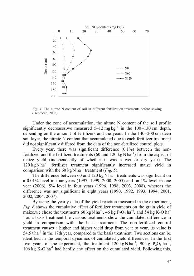
47

N0N60N120

Dep

th (c

m)

Soil NO3-content (mg kg-1) 0 10 20 30 40 50 60 70

0

20

40

60

80

100

120

140

160

180

200

Fig. 4. The nitrate N content of soil in different fertilization treatments before sowing (Debrecen, 2008) Under the zone of accumulation, the nitrate N content of the soil profile

significantly decreases,we measured 5–12 mg kg–1 in the 100 –130 cm depth, depending on the amount of fertilizers and the years. In the 140 –200 cm deep soil layer, the nitrate N content that accumulated due to each fertilizer treatment did not significantly differed from the data of the non-fertilized control plots.

Every year, there was significant difference (0.1%) between the non-fertilized and the fertilized treatments (60 and 120 kg N ha–1) from the aspect of maize yield (independently of whether it was a wet or dry year). The 120 kg N ha–1 fertilizer treatment significantly increased maize yield in comparison with the 60 kg N ha–1 treatment (Fig. 5).

The difference between 60 and 120 kg N ha–1 treatments was significant on a 0.01% level in four years (1997, 1999, 2000, 2005) and on 1% level in one year (2006), 5% level in four years (1996, 1998, 2003, 2008), whereas the difference was not significant in eight years (1990, 1992, 1993, 1994, 2001, 2002, 2004, 2007).

By using the yearly data of the yield reaction measured in the experiment, Fig. 6 shows the cumulative effect of fertilizer treatments on the grain yield of maize.we chose the treatments 60 kg N ha–1, 46 kg P2O5 ha–1, and 54 kg K2O ha–

1 as a basis treatment the various treatments show the cumulated difference in yield in comparison with the basis treatment. The non-fertilized control treatment causes a higher and higher yield drop from year to year, its value is 54.5 t ha–1 in the 17th year, compared to the basis treatment. Two sections can be identified in the temporal dynamics of cumulated yield differences. In the first five years of the experiment, the treatment 120 kg N ha–1, 90 kg P2O5 ha–1, 106 kg K2O ha-1 had hardly any effect on the cumulated yield. Following this,

48

yield increased from year to year, and the yield surplus was 10.8 t ha–1 in the 17th year of the experiment, compared to the basis treatment.

Non-fertilised 60 kg N ha–1 120 kg N ha–1

Fertilisation (kg ha–1)

Yie

ld (t

ha–1

) 16151413121110 9 8 7 6 5 4 3 2 1 0

Fig. 5. The effect of fertilization on maize yield (Debrecen, 1990–2008).

20082007200620052004200320022001200019991998199719961994199319921990

non-fertilised 60 kg N ha-1 120 kg N ha-1

Com

mul

ated

yie

ld d

iffer

ence

(t h

a–1)

1990

19

92

1993

19

94

1996

19

97

1998

19

99

2000

20

01

2002

20

03

2004

20

05

2006

20

07

2008

Non fertilised 60 kg N ha–1 120 kg N ha–1

Years

20

0

– 20

– 40

– 60

Fig. 6. Cumulated yield difference of the various treatments in comparison with the basis treatment (Debrecen, 1990–2008)

49

3.3. Effect of fertilization and precipitation on maize yield

Multifactoral analysis of variance of yield During the joint analysis of variance,we examined the effect of the two independent variables (1: fertilization, 2: precipitation) on yield at the same time. Based on the significance levels, both factors had significant effects on yield (p < 0.001) and the interaction of the two factors was also significant (p < 0.05). Fertilization is responsible for nearly twice as much of the standard deviation of yield as precipitation, that is the effect of fertilization treatments on maize yield is much more significant than that of precipitation (Table 2). Based on the value of R2, independent variables are 56.8% responsible for the variance of the dependent variable.

Table 2. The (combined) variance analysis of the effect of fertilization and precipitation, also considering years, yield t ha–1 (Debrecen, 1990 –2008)

Factors Mean Square

Degrees of Freedom F value Sig

Fertilization 706,9 2 237,7 0,000 Precipitation 363,8 1 122,3 0,000 Fertilization × Precipitation 11,7 2 3,9 0,049 Error 3,0 486

R squared = 0,568 (Adjusted R Squared = 0,523)

Effect of fertilizer treatments in dry and wet years In dry years,we analysed the effect of fertilizer treatments on the dependent

variable by the non-parametric equivalent of one-way ANOVA (Kruskal-Wallis) andwe established that the effect was significant (p < 0.01). The non-fertilized and fertilized (60 and 120 kg N ha–1) treatments significantly differed from each other: at the 60 kg N ha–1 fertilizer level, the average yield obtained was higher by 2.82 t ha–1 than in the case of non-fertilized treatments, whereas if 120 kg N ha–1 is applied, the yield obtained was higher by 3.25 t ha–1 (p < 0.001) in comparison with non-fertilized conditions.we compared median values by Mann-Whitney test and found that there was no significant difference between 60 and 120 kg N ha–1 treatments.

In wet years,we used variance analysis to show that different fertilizer treatments have different effects on maize yield (p < 0.01). As for the 60 kg N ha–1 fertilizer treatment, the utilization of fertilizer was significantly higher by 3.69 t ha–1 than in the case of the non-fertilized treatment, whereas this value was 4.46 t ha–1 when 120 kg N ha–1 was applied (p < 0.001). No statistical difference could be shown between the 60 and 120 kg N ha–1 fertilizer treatments.

50

The effect of precipitation in different fertilizer treatments After examining the normality of yield in every fertilizer treatment,we

established that the variable has a normal distribution on two fertilizer levels. Concerning these treatments,we performed variance analysis to examine the effect of precipitation on yield, whereaswe applied a non-parametric test in the case of non-fertilized treatment.

As for the non-fertilized treatment and the two different NPK effects, the amount of precipitation significantly affected yield (p < 0.001) and significantly higher yields were obtained in years when there was more precipitation. In the non-fertilized treatment, the yield was 1.50 t ha–1 higher in wet years, whereas it was 2.36 t ha–1higher in the case of the fertilizer treatment 60 kg N ha–1 and by 2.70 t ha–1 in the case of the fertilizer treatment 120 kg N ha–1 than in dry years.

During the wet years, the yield increasing effect of fertilization is higher than in dry years. The yield increment was 0.86 t ha–1 in the case of non-fertilized treatments and the 60 kg N ha–1 treatment, whereas it was 1.21 t ha–1 in the case of 120 kg N ha–1.

I classified the years by average yield into four groups using a hierarchic cluster analysis based on combination. Of the examined 17 years, very low yields were obtained in three years, low yields were obtained in seven years, whereas there were high yields in three years and very high yields in three years (Fig. 7).

C A S E

Label Num 1990 1 2003 12 2002 11 2000 9 2006 15 1993 3 1996 5 1994 4 2007 16 1992 2 1997 6 2004 13 2001 10 2005 14 1998 7 1999 8 2008 17

Rescaled Distance Cluster Combine

0 5 10 15 20 25 +---------+---------+---------+---------+---------+

Fig. 7. Hierarchical cluster analysis based on combination on the basis of the average maize yield (Debrecen, 1990–2008).

51

Acknowledgement—This work was supported by the National Office for Research and Technology NKTH 00210/2008, TÁMOP 4.2.1./B–09/1/KONV–2010–0007 and TÁMOP 4.2.2./B–10/1-2010-0024.

References

Aguilar, M., Borjas, F., Espinosa, M., 2007: Agronomic response of maize to limited levels of water under furrow irrigation in southern Spain. Spanish Agric. Res. 5, 587–592.

Barrov, E.M., Hulme, M., Semenov, M.A., Brooks, R.J., 2000: Climate change scenarios. In: Climate Change, Climatic Variablility and Agriculture in Europe (eds.: Downing, T.E., Harrison, P.A., Butterfield, R.E., Londsdale, K.G.) Europcan Commision, Brussel.

Berényi, D., 1956: A cukorrépa termésátlaga és az időjárási elemek közötti összefüggés. Acta Univ. Debr. 3, 229−249.

Claassen, M.M., Shaw, R.H., 1970: Water deficit effects on corn. II. Grain components. Agron. J. 62, 652–655.

Davidson, H.R., Campbell, C.A., 1983: The effect of temperature, moisture and nitrogen on the rate of development of spring wheat as measured by degree days. Can. Plant Sci. 63, 833–846.

Delphin, J-E., 2000: Estimation of nitrogen mineralization in the field from an incubation test and from soil analysis. Agron. Sustain. Dev. 20, 349–361.

Díez-López J.A., Hernaiz-Algarra, P., Arauzo-Sánchez, M., Carrasco-Martín, I., 2008: Effect of a nitrification inhibitor (DMPP) on nitrate leaching and maize yield during two growing seasons. Spanish Agric. Res. 6, 294–303.

Gallagher, J.N., 1979: Field studies of cereal leaf growth: I. Initation and expansion in relation to temperature and ontogeny. J. Exp. Bot. 30, 625–636.

Hansen, E.M., Djurhuus, J., 1996: Nitrate leaching as affected by long-term N fertilization on a coarse sand. Soil Use Manage. 12, 221–228.

Ichir, L.L., Ismaili, M., Hofman, G., 2003: Recovery of 15N labeled wheat residue and residual effect of N fertilization in a wheat-wheat cropping system under Mediterranean conditious. Nutr.Cycl. Agroecosys. 66, 201–207.

Kavlen, D.L., Kramer, L.A., Logsdon, S.D., 1998: Field-scale nitrogen balances associated with long-term continous corn production. Agron. J. 90, 644–650.

Kiesselbach, T.A., 1950: Progressive development and seasonal variation of corn crop. Univ. Nebraska Bull., 166.

Körschens, M., 2006: The importance of lond-term experiments for soil science and environmental research – a review. Plant Soil Environ. 52, (Special Issue) 1–8.

Láng, G., 1976: Szántóföldi növénytermesztés. Mezőgazdasági Kiadó, Budapest. Lauer J., 2003: What happens within the corn plant when drought occurs. Univer. Wisconsin Ext.,

http://www.uwex.edu/ces/ag/issues/drought2003/corneffect.html Márton, L., 2002: Az évhatás elemzése az északkelet-magyarországi, nyírlugosi műtrágyázási

tartamkísérletben. A természetes csapadék és a tápanyagellátottság hatása a burgonya (Solanum tuberosum L.) termésére. Növénytermelés 51, 71−87.

Mckenney, M.S., Rosenberg, N.J., 1993: Sensitivity of some potential evapotranspiration estimation methods to climate change. Agric. Forest Meteorol. 64, 81–110.

Nagy, J., 2008: Maize production. Akadémiai Kiadó, Budapest, 391. Nakamura, K., Harter, T., Hirono, Y., Hirono, H., Mitsuno, T., 2004: Assessment of root zone nitrogen

leaching as affected by irrigation and nutrient management practices. Vadose Zone J. 3, 1353–1366. Nield, R.E., Seeley, M.W., 1977: Growing degree days predictions for corn and sorghum development

and some applications to crop production in Nebraska. Nebr. Agric. Exp. Stn. Res. Bull. 280. Lincoln, Ne.

52

Ordofiez, R., Giraldez, J.V., Gonziiez, P., 1990: Nitrogen use on irrigated farms in the Guadalquivir Valley: approach to a rational design after soil column leaching experiments. International Symposium, Nitrate-Agriculture-Eau. Proc. ( ed. :R. Calvet), Paris, 437–443.

Penman, H.L., 1948: Natural evaporation from open water, bare soil and grass. Proc. R. Soc. Lond. 193, 120–145.

Quattar, S., Jones, R.J., Crookston, R.K., Kajelou, M., 1987: Effects of water deficit during grain filling on the pattern of maize kernel growth and development. Crop Sci. 27, 730–735.

Ramos, C., Varela, M., 1990: Nitrate leaching in two irrigated fields in the region of Valencia (Spain). International Symposium, Nitrate-Agriculture-Eau. Proc. ( ed.: R. Calvet), Paris, 335–345.

Shaw, R.H., 1977: Climatic requirement. In: Corn and corn improvement (ed.: Sprague, G.F.), Amer.Soc.Agron.Inc. Publisher, Madison, Wisconsin, 774.

Smith, W.C., Betrán, J., Runge, E.C.A. (eds), 2004: Corn. Origin, History, Technology, and Production. Hoboken, NJ: John Wiley, 949.

Szász G., 1977: Formulae of Calculating Evapotranspiration and their Application in the Practice of Hungary. I.C.I.D., Internat round Table conf. On „Evapotranspiration”. Question 3, 1–13.

Thornthwaite, C.W., 1948: An approach toward a rational classification of climate. Geogr. Rev. 38, 5–94.

Westgate, M.E., Boyer,J.S., 1986: Reproduction at low silk and pollen water potentials in maize. Crop Sci. 26, 951–956.

Westgate, M.E., Grant, D.L.T., 1989: Water deficits and reproduction in maize responses of the reproductive tissues to water deficits at anthesis and mid-gain fill. Plant Physiol. 91, 862–867.

53

IDŐJÁRÁS Quarterly Journal of the Hungarian Meteorological Service

Vol. 116, No. 1, January–March 2012, pp. 53–64

The efficiency of natural foliar fertilizers

Róbert Víg1*, Attila Dobos1, Krisztina Molnár2, and János Nagy1

1Research Group of Cultivation and Regional Development,

Hungarian Academy of Sciences,University of Debrecen Böszörményi út 138.H-4032 Debrecen, Hungary

2Institute for Land Utilisation, Technology and Regional Development,

Center of Agricultural Sciences and Engineering, University of Debrecen Böszörményi út 138, H-4032 Debrecen, Hungary

*Corresponding author; E-mail: vr.esoxipmail.hu

(Manuscript received in final form February 3, 2012)

Abstract—In the light of the agricultural development, microbiological products have increasing significance, since it is possible to improve soil fertility and tolerance of cultivated crops, and the use of chemical fertilizer can be reduced.

The efficiency of natural foliar fertilizers was examined in a three-year long analysis (2006–2008) in the southern production area of Hajdúszoboszló on meadow chernozem soil. During the examinations, the primary question was whether the foliar fertilizers Natur Vita (Chlorella vulgaris and Spirulina platensis), Natur Plasma (Chlorella spp.), and Amalgerol Premium (alginate, mannitol, laminarin etc.) provide further yield increase on top of basic fertilisation in maize population and stubble field treatments. The efficiency of products was tested in hybrid seed production, and the examinations were extended to potato production, too.

During the statistical evaluation of the research results, it was established that the use of the tested foliar fertilizers improve the vital conditions of the hybrid seed production. Depending on the applied treatment, foliar fertilizers provide further yield increase on top of basic fertilization, and their combined use does not result in significantly higher yield than in the case of applying products individually. Key-words: maize, SPAD, foliar fertilizer, efficiency

1. Introduction

One of the key issues of sustainable agriculture is the maintenance of soil fertility (Reeves, 1997; Arshad and Martin, 2002; Gosling and Shepherd, 2005), but the strongly chemicalized farming method which neglects production site

54

conditions could lead to harmful processes in the soil that results in the reduction of soil fertility (Schwab, 1990; Kim et al., 2000; Nagy, 2006, 2007). Such negative effects are the deterioration of the fertile soil (erosion, deflation) (Evans, 2005; Deumlich et al., 2006), soil contamination (Hansen et al., 2000), reduction of the organic matter content and biological activity of the soil (Dawe et al. 2003; Loveland and Webb, 2003), salinification (Liang et al., 1996), and deterioration of the soil structure (Lupwayi et al., 2001; Bronick and Lal, 2005).

Biofertilizers could have significant role in sustainable agroecosystems, as they help to maintain soil fertility (Kannaiyan, 2002; Wu et al., 2005; Kincses et al., 2009), and they can contribute to yield increase without imposing a chemical load on the environment (Gould, 1990).

Biofertilizers are the products which contain microorganisms that have a beneficial effect on the nutrient extraction, plant growth, and development (Vessey, 2003). These products could either be plant growth-promoting rhizobacteria (PGPR) (Kloepper et al., 1989; Döbereiner, 1997; Cong et al., 2009), arbuscular mycorrhizal fungi (AMF) (Duffy and Cassells, 2000; Douds et al., 2006), and algae (Nisha et al., 2007).

The bacteria living in the soil (PGPR) have a beneficial effect on crops and they play a significant role in the protection against phytopathogens, nitrogen fixation, nutrient extraction (Vessey, 2003), improve the development of the favorable soil structure (Kohler et al., 2006), and increase the resistance of crops to environmental stress factors (Sturz and Nowak, 2000; Gajdos, 2009). The mycorrhizal fungi that live in symbiosis with plant roots make immobile elements available to plants, they help water uptake and increase resistance to pathogens (Smith and Read, 1997).

Algae have outstanding nitrogen fixation ability which makes it possible to use them as a fertilizer. Similarly to farmyard manure, the proportion of organic matter is high in algae (400 units), while the ratio of potassium is satisfactory (27 units) and that of phosphorus is small (2 units); therefore, algae fertilization needs to be supplemented with phosphorus. In addition to the favorable nitrogen supply ability, the yield increasing efficiency is also due to the microelements (Fe, Cu, Mn, Zn), vitamins auxins and gibberellins, which can be found in algae (Péterfi, 1977). The algae varieties tested as biofertilizers primarily belong to the branch of blue-green algae (Cyanophyta) and green algae (Chlorophyta) (Tripathi et al., 2008; Hernandez et al., 2009).

2. Material and methods

The selected plots were uniform from the aspect of soil characteristics. The localization of experimental areas was performed with Trimble GPS Pathfinder ProXH and ArcPad 7.0 software, and the polygons of the plots were aligned to a digitalized genetic soil map in ArcGis 9.1. The range of plots suitable for the

55

examination was determined on the basis of the number of soil types and subtypes on the plot, as well as their regional distribution. Examinations were established on chernozem soil in all cases.

In the area selected for the examination, the soil sampling was done by using an Eikelkamp manual borer on every 4 hectares, in average in the upper 0 –30 cm layer of the soil, using Trimble GPS Pathfinder ProXH and ArcPad 7.0 software based on a genetic soil map in the spring and autumn of 2006.

The soil of the examined plots belongs to the clayey adobe physical soil group. The soil is slightly acidic, it is moderately chalky and it has low salt content, adequate humus content, average nitrogen content and low zinc content. The area of maize production in 2006 and 2007 was moderately supplied with phosphorus and potassium, while the plot used for hybrid seed production in 2008 was poorly supplied with these two elements (Table 1).

In all three years, the examinations were performed in hybrid seed production area on which basic fertilisation was applied. Interplanting was used. The previous crop was maize in all cases. The vegetable remains were chopped by stem crushing and disking (early-mid September), and the crushed stem remains were incorporated into the soil in the autumn (mid-late September) with 35 cm deep ploughing at the early stage of seedbed preparation with a compactor in early April. Sowing took place in late April – early May by interplanting technique. Female rows were sown with a Monosem sowing machine, while we used an Optima sowing machine in the case of male rows.

130–160 kg ha–1 nitrogen, 80 – 85 kg ha–2 phosphorus and 70 – 80 kg ha–1 potassium were applied as basic fertilizer. 10 – 15% of phosphorus, potassium, and nitrogen were applied in the autumn in the form of complex fertilizer and 85 – 90% of nitrogen was applied in the spring before seedbed preparation.

Table 1. Mean values of the soil analysis results of the experimental areas

Soil parameters Year of examination 2006 2007 2008

pH(H2O) 8.3 8.2 8.1 CaCO3 (mg kg–1) 3.1·104 2.2·104 1.6·104 Total water-soluble salt content (mg kg–1) 130 130 130 Humus (mg kg–1) 3.11·104 3.12·104 2.92·104 Total nitrogen (mg kg–1) 1750 1814 1701 AL-P2O5 (mg kg–1) 161 169 84 AL-K2O (mg kg–1) 287 286 218 KCl-EDTA Zn (mg kg–1) 1.45 1.62 1.17

The treated and the control plots were planned to be 12 m wide, and the sampling points were selected in four replications with ArcGis 9.1 software.

During the examinations, the efficiency of foliar fertilizers containing algae and algae extracts was evaluated. Natur Plasma is a microbiological product which contains living Chlorella spp. species (3 x 107 per ml) (Haller, 2009). This

56

foliar fertilizer contains 0.3 w w–1% dry matter, 550 mg l–1 nitrogen, 150 mg l–1 phosphorus, 1146 mg l–1 magnesium, and 70 mg l–1 zinc. The variant of Natur Plasma enriched with zinc was also used, as its zinc content is 530 mg l–1 higher. Natur Vita contains Chlorella vulgaris and Spirulina platensis in powdered form (Haller, 2009). This foliar fertilizer contains 90 w w

–1% dry matter, 15 g 100 g –1 nitrogen, and 1.3 g 100g

–1 phosphorus and potassium. Furthermore, the foliar fertilizer called Amalgerol Premium was also tested. This product contains algae extracts (alginate, mannitol, laminarin), and it contains 17.2 ww

–1% dry matter, 5550 mg l–1 nitrogen, 614 mg l–1 phosphorus, and 3649 mg l–1 potassium.

250 g ha–1 Natur Vita, 6.4 l ha–1 Natur Plasma and Natur Plasma enriched with zinc, and 2.5 l ha–1 Amalgerol Premium were used with 250 l ha–1 water in population treatment. The products were applied on two occasions (at the 5 – 8 leaf stages and 1–1.5 weeks before tasseling) in similar doses by using a Berthoud Boxer 3000 sprayer. In the third year (2008), Amalgerol Premium (5.0 l ha-1) was applied in combined treatment at the 2 –3 leaf stages and Natur Plasma (5.0 l ha–1) was applied at the 5 – 8 leaf stages one week before tasseling.

Examined products:

• Natur Plasma (Chlorella algae concentrate enriched with nutrients)

• Natur Vita (Powdered version of Chlorella algae concentrate)

• Amalgerol Premium (vegetable volatile oils, alginate, mannitol, laminarin, algae extract, macro- and microelements)

In the stubble field treatment (October 2006), Amalgerol Premium was applied in 2.0% concentration (6.0 l ha–1 with 300 l ha–1 water) and Natur Plasma was applied in 3.2% concentration (10 l ha–1 with 300 l ha–1 water). The treatment was carried out on a maize stubble field ,and it was preceded by stem crushing and disking. The application of products was performed directly onto the soil surface which was then followed by shallow (5–10 cm) disking. The effect of stubble field treatment was evaluated in a hybrid seed production in 2007.

Before harvesting, yield samples were collected in four replications per treatment from 10 plants per replication, then the efficiency of foliar fertilizers was evaluated on the basis of fertility (number of grains per stem) and yield (g per stem).

The chlorophyll content of leaves provides information about the physiological condition of plants, since the different natural and anthropogenic stress factors affect the amount of chlorophyll (Carter 1994). The amount of chlorophyll can be easily measured in the visible and ultraviolet range with non-destructive optical methods (Markwell et al., 1995; Sims et al., 1995; Cartelat et al., 2005). The Minolta SPAD-502 chlorophyll meter determines the relative chlorophyll content of leaves by means of the absorption of 650 nm wavelength light. In order to do that, the SPAD-502 meter uses infrared light in the

57

940 nanometer wavelength range as reference. The device expresses the relative chlorophyll content in SPAD values which is calculated from the intensity of the red and infrared light transmitted through the leaf (Minolta Camera Co. Ltd., 1989). In order to evaluate the effect of treatments on the crop condition, SPAD measurements were performed with the Minolta SPAD-502 meter in 2008. Ten measurement points were proportionally divided along the entire leaf-blade on the left and right sides (5–5 points), using the 6th–7th leaves on 10 stems per sampling point. The measurements were carried out on three occasions; before the first treatment (June 5, 2008), between the two treatments (July 11, 2008), and after the second treatment (August 6, 2008).

During the statistical evaluation of the foliar fertilizer treatments, the normality of the distribution of fertility, yield, and SPAD values were examined by the Kolmogorov-Smirnov test, and the identity of variances was evaluated by the Levene’s test. The examination of normality showed normal distribution in all cases; therefore, a parametric test was selected to compare means. The simultaneous comparison of mean values was done by the Duncan’s test at a 5% inaccuracy level).

Of the years of examination, 2006 and 2007 were too dry for maize, while 2008 was favorable. The number of sunny hours in the growing season (1618 –1779 hours), its effective heat sum (1437–1660 oC), average temperature (17.6–18.7 oC), rainfall (348–406 mm) and the annual precipitation (545–629 mm) was favourable for maize. The distribution of rainfall was unfavourable in all three years at the time of tasseling (July). The monthly amount of precipitation (61–65 mm) was in the optimal range for maize (50–80 mm), but 82% (50 mm) of the monthly precipitation in 2006 was measured in one day (July 22, 2006), 72% (47 mm) of the rainfall in July 2007 was measured in two days (July 4 and 5, 2007), while 68% (29 mm) of the monthly precipitation in 2008 was measured in two days (July 4, 2008 and July 7, 2008).

The average 14-hour relative atmospheric humidity at the time of pollen spreading (July) was 46% in 2006, 44% in 2007, 59% in 2008. In 2006 and 2007, the number of days with relative humidity under 45% in July was high (19–21 days); therefore, 2006 and 2007 were less favorable than 2008 from the aspect of fertility. The differences in yield of the various crop years were evaluated with Welch and t tests, depending on whether the Levene’s test showed the identity or difference of the variances.

3. Results of the experiments

In the first year of the examination (2006), the yield increasing efficiency of Natur Plasma was examined in population treatment on four treated and four control plots. During the evaluation of efficiency, the effect on yield was examined as expressed in grains per stem (number of grains per stem) and g per

58

stem. As a result of the treatment, the number of grains improved by 59 grains per stem and yield increased by 14.2 g per stem (0.9 t ha–1) in comparison with the control.

The normality of the fertility and yield of the control and treated plots was examined with the Kolmogorov-Smirnov test and the identity of variances was checked with the Levene’s test. The examined variables had normal distribution and the same variance; therefore, an independent two-sample t-test was used. The t-test showed significant differences (p < 0.05) in the number of grains per crop and yield between the treated and control populations; therefore, the Natur Plasma treatment had a favorable effect on the fertility and yield on the hybrid seed production (Table 2).

Table 2. Results of the t-test concerning grain number per plant (number per stem) and yield (g per stem) (2006)

Grain number (number per stem) Yield (g per stem)

Mean t value df Mean t value df

Natur Plasma 149 3.25* 78 35.7 3.26* 78 Control 90 21.5

* p < 0.15, df = number of degrees of freedom

In the second year of examination (2007), the efficiency of natural foliar

fertilizers (Natur Plasma, Natur Plasma enriched with zinc, Natur Vita, Amalgerol Premium) was examined in population treatment and stubble field treatment. During the evaluation of efficiency, the effect of these fertilizers on the number of grains per plant (number of grains per stem) and yield (g per stem) was evaluated.

The average number of plant was lower on the control plot than in the population treatments, and the number of grains measured in the stubble field treatments was similar to that of the control plots. Among the different population treatments, the highest grain number was observed on the areas treated with Natur Plasma and Natur Plasma enriched with zinc. In comparison with the control plot, the number of grains per plant increased by 0–26 grains per stem in the stubble field treatments, while it increased by 41–48 grains per stem in population treatments. Based on the Duncan’s test, the number of grains per plant measured in the stubble field treatments did not differ significantly from the control population, but significantly higher (p < 0.05) grain number was observed in all population treatments than in the control population and the Amalgerol Premium stubble field treatment. In the population treatments with Natur Plasma and Natur Plasma enriched with zinc, the number of grains per stem was significantly higher (p < 0.05) than in the case of areas sprayed with Natur Vita and Amalgerol Premium. There was no significant difference between the population treatments with Natur Plasma, Natur Plasma enriched

59

with zinc, the population treatment with Natur Vita and Amalgerol Premium, and the stubble field treatment with Natur Plasma (Table 3).

The average yield was the lowest in the Natur Plasma stubble field treatment (2.0 t ha–1) and in the control population (2.2 t ha–1), while the highest values were observed in the areas treated with Natur Plasma enriched with zinc (2.9 t ha–1), Natur Vita (2.8 t ha–1), and Natur Plasma (2.7 t ha–1). The population treatment with Amalgerol Premium (2.5 t ha–1) and the stubble field treatment with the same fertilizer (2.5 t ha–1) had nearly similar results, but they were below those that were measured in the population treatments of the other examined products. In comparison with the control population, the stubble field treatments resulted in 0.1– 4.7 g per stem (0.1– 0.3 t ha–1), while the population treatments increased the yield by 5.4 –11.9 g per stem (0.3– 0.7 t ha–1). Based on the significance results of the Duncan’s test, it was established that the yield obtained in population treatments and the yield measured in the stubble field treatment with Amalgerol Premium were significantly higher (p < 0.15) than the yield measured in the control population, while the stubble field treatments done with Natur Plasma is not significantly different from that of the control population. Based on the significance results, there were no obvious differences between the treatments. The yield obtained in the stubble field and population treatments with Amalgerol Premium did not differ significantly from those of the population treatments with Natur Vita and Natur Plasma. The yield obtained in the treatment with Natur Plasma enriched with zinc was significantly higher (p < 0.05) than the yield of the control population and the stubble field treatment, but its yield was the same as that of the population treatments with Amalgerol Premium, Natur Plasma, and Natur Vita (Table 3).

Based on the results obtained in 2007, the population treatments had a favorable effect on the fertility and yield of the hybrid seed production, while the differences between the effects of stubble field treatments and population treatments were not clearly expressed; therefore, further examinations are necessary.

Table 3. The effect of treatments on the grain number per plant (number per stem) and yield (g per stem) (2007)

Treatments Grain number Yield n

Control 149 c 33.3 c 40 Amalgerol Premium (s) 143 c 38.1 b 40 Natur Plasma (s) 175 bc 31.1 c 40 Natur Plasma (p) 233 a 42.1 ab 40 Natur Plasma enriched with zinc (p) 224 a 45.2 a 40 Natur Vita (p) 190 b 42.7 ab 40 Amalgerol Premium (p) 191 b 38.7 ab 40 F value 9.10 * 4.94 *

* p < 0.15, p = population treatment, s = stubble treatment, n = element number

60

In the third year of the examination (2008), the efficiency of natural foliar fertilizers (Natur Plasma, Natur Vita, Amalgerol Premium) was examined in population treatment. During the evaluation of efficiency, the effect of these fertilizers on the SPAD values, the number of grains per plant (number of grains per stem), and the yield (g per stem) were evaluated.

The differences between the selected plant populations expressed in SPAD values were evaluated before the first spraying. The lowest average SPAD value was measured in the population selected for combined treatment, while the highest average value was obtained in the second control population. The SPAD value of the plot to be treated with Amalgerol Premium and the first control was above 32.0, but it was lower than the average values measured in the areas selected for Natur Vita and Natur Plasma treatments. Based on the Duncan’s test, it was established, that the SPAD values measured in the second control population were significantly higher (p < 0.05) than in the other areas, but the SPAD values of the first control area and the plots selected for treatments were shown to be identical; therefore, the effects of treatments were evaluated in comparison with the first control (Table 4).

Table 4. The effect of treatments on the SPAD value of maize leaves (2008)

Treatments Before the 1st treatment

After the 1st treatment

After the 2nd treatment n

Control 1 32.9 b 47.1 b 35.8 c 48 Control 2 36.1 a - - 48 Natur Plasma 33.8 b 50.2 a 38.5 b 48 Natur Vita 33.1 b 49.6 a 38.4 b 48 Amalgerol Premium 32.8 b 50.5 a 38.8 b 48 Combined treatment 31.8 b 50.9 a 41.3 a 48 F value 4.46 * 5.34 * 5.38 *

* p < 0.05, n = element number

After the first treatment, the lowest average SPAD value was measured in the control population, while the highest value was obtained in the combined treatment. There was only a slight difference (0.4 –1.3) between the values measured in the population treatments. After the first treatment, the Duncan’s test showed significant difference (p < 0.05) between the SPAD results of the control population and the treatments, while there was no significant difference between the SPAD values of the treatments (Table 4).

After the second treatment, the lowest average SPAD value was measured in the control plot, while the highest one was obtained in the combined treatment. The average SPAD values of the plots treated with Natur Vita, Natur Plasma, and Amalgerol Premium did not reach 40.0. The Duncan’s test showed that the SPAD measurements performed in the treatments were significantly higher (p < 0.05) in comparison with the control plot. There was no significant

61

difference between the treatments with Natur Vita, Natur Plasma, and Amalgerol Premium, but their average SPAD values were significantly lower (p < 0.05) than the average SPAD value of the combined treatment (Table 4).

The lowest grain number per stem was counted in the control population and the Natur Vita treatment, while the highest average value was obtained in the combined treatment. The extent of fertility in the case of Natur Plasma and Amalgerol Premium was lower than the average values in the combined treatment. In comparison with the control plot, the number of grains per plant increased by 9–39 grains per stem, but the Duncan’s test did not show any significant difference between the treated and non-treated populations (Table 5).

The lowest average yield was obtained in the control population (3.2 t ha–1), while the highest value was measured in the combined treatment (3.9 t ha–1). The average yield of the plots treated with Natur Vita (3.7 t ha–1), Natur Plasma (3.8 t ha–1), and Amalgerol Premium (3.8 t ha–1) exceeded the average yield of the control population, but they were lower than the value measured in the combined treatment. The Duncan’s test showed significant differences (p < 0.05) between the yield of the control population and the treatments, but it did not show any significant difference in the average yield of the different treatments. Fertilization with the examined products resulted in 8.1–11.3 g per stem (0.5 – 0.7 t ha–1) yield increase in comparison with the control population (Table 5).

During the statistical evaluation of the examination results, it was established that the natural foliar fertilizers had a favorable effect on the SPAD values of the hybrid seed production, and this effect was even more expressed after the second treatment. In contrast with 2007, the treatments did not increase the grain number significantly in 2008, but they resulted in significant yield increase in comparison with the control population.

Table 5. The effect of treatments on the grain number per plant (number per stem) and yield (g per stem) (2008)

Treatments Grain number (number per stem) Yield (g per stem) n

Control 1 251 a 49.2 b 40 Natur Plasma 272 a 57.7 a 40 Natur Vita 260 a 57.3 a 40 Amalgerol Premium 283 a 58.9 a 40 Combined treatment 290 a 60.5 a 40 F value 1.59 n.s 2.95 *

* p < 0.05, n.s. = no significant difference, n = element number

2006 and 2007 were unfavorable years from the aspect of fertility, while

2008 was a favorable year. The average 14-hour relative atmospheric humidity at the time of pollen spreading (July) was lower in 2006 and 2007 (44 – 46%)

62

than in 2008 (59%), while the number of days in July with the relative humidity below 45% were more in 2006 and 2007 (19 –21 days) than in 2008.

Comparing the results of 2006 and 2007 with those of 2008, it was established that the number of grains per plant and yield obtained in the control populations and the treated populations in the drought years (2006, 2007) were significantly lower (p < 0.001) than in the year which was more favorable from the aspect of fertility (2008), and the increase in grain number and yield in comparison with the control population was larger than in 2008 (Table 6).

Table 6. The effect of treatments in different crop years

Years of examination Mc df t value Mpt df t value MDc

Grain number (number per stem) (3) 2006-2007 120 116 9.13* 180 358 9.43* 60 2008 251 276 25

Yield (g per stem) (4) 2006-2007 27.4 116 7.82* 39.0 358 10.42* 11.6 2008 49.5 58.6 9.1

* p < 0.05, Mk = mean of control populations, Mpt = mean of population treatments, MDc = average difference in comparison with the control, df = number of degrees of freedom

4. Conclusions

During the statistical evaluation of the examination results, it was established that the use of the tested foliar fertilizers improved the condition of the crop population. Depending on the applied treatment, they provide further yield increase in addition to the basic fertilization, and their combined use does not result in significantly higher yield than the individual application of each product. Based on the results, it is assumed that natural foliar fertilizers are able to substitute basic fertilization to a certain extent; therefore, it is necessary to examine this issue under small and large plot conditions.

The application of the examined products as foliar fertilizers resulted in more favorable yield increase in the drought years than in 2008, which was a less favorable year from the aspect of fertility. This result leads to the conclusion that the yield increasing effect of algae- and algae extract-based foliar fertilizers is a result of their crop conditioning effect, which is more expressed in stress (e.g. atmospheric drought) than under optimal conditions. Consequently, the cost-effectiveness of these treatments could be more favorable in stress.

Field experiments on foliar fertilization are more difficult to carry out because sometimes the treated and the control plots are not uniform even before the treatment. Based on the results of the SPAD measurements performed before the first foliar fertilizer treatment, it can be examined whether the conditions of

63

the crop populations selected as control or treated populations are identical or different. Therefore, during the evaluation of the obtained yield and based on the preliminary SPAD measurements, it is possible to compare the treatments to the control population in which the plant condition was identical to the populations selected for treatment even before the treatment itself. The advantage of this method is that the yield increasing potential of foliar fertilizers can be accurately evaluated, which provides an opportunity to compare foliar fertilizers in a rational way. The disadvantage of this method is that the obtained results are slightly higher than the yield increase which can be expected under controlled field trial conditions that results from the fact that the yield loss resulting from the heterogeneity of the crop population is excluded during the examination; therefore, the cost-efficiency based examination of the large-scale use of these products is indispensable.

Acknowledgements—We would like to thank István Farkas, Sándor Bartha, Csaba Varga, and Szabolcs Munkácsi for their help in establishing the experiments.

Refrences

Arshad, M.A. and Martin S., 2002: Identifying critical limits for soil quality indicators in agro-ecosystems. Agr. Ecosyst. Environ. 88, 153–160.

Bronick, C.J. and Lal, R., 2005: Soil structure and management: a review. Geoderma 124, 3–22. Cartelat, A., Cerovic, Z.G., Goulas, Y., Meyer, S., Lelarge, C., Prioul, J.L., Barbottin, A., Jeuffroy, M.H.,

Gate, P., Agati, G., Moya, I., 2005: Optically assessed contents of leaf polyphenolics and chlorophyll as indicators of nitrogen deficiency in wheat (Triticum aestivum L.). Field Crops Res. 91, 35–49.

Carter, G.A., 1994: Ratios of leaf reflectances in narrow wavebands as indicators of plant stress. Int. J. Remote Sens. 15, 697–703.

Cong, P.T., Dung, T.D., Hien, T.M., Hien, N.T., Choudhury, A.T.M. A., Kecskés, M.L., and Kennedy, I.R., 2009: Inoculant plant growth-promoting microorganisms enhance utilisation of urea-N and grain yield of paddy rice in southern Vietnam. Eur. J. Soil Biol. 45, 52–61.

Dawe, D., Dobermann, A., Ladha, J.K., Yadav, R.L., Bao, L., Gupta, R.K., Lal, P., Panaullah, G., Sariam, O., Singh, Y., Swarup, A., and Zhen, Q.X., 2003: Do organic amendments improve yield trends and profitability in intensive rice systems? Field Crop. Res. 83, 191–213.

Deumlich, D., Funk, R., Frielinghaus, M., Schmidt, W.A., and Nitzsche, O., 2006: Basics of effective erosion control in German agriculture. J. Plant Nutr. Soil Sc. 169, 370–381.

Douds Jr., D.D., Nagahashi, G., Pfeffer, P.E., Reider, C., and Kayser, W.M., 2006: On-farm production of AM fungus inoculum in mixtures of compost and vermiculite. Bioresource Technol. 97, 809–818.

Döbereiner, J., 1997: Biological nitrogen fixation in the tropics: Social and economic contributions. Soil Biol. Biochem. 29, 771–774.

Duffy, E.M. and Cassells, A.C., 2000: The effect of inoculation of potato (Solanum tuberosum L.) microplants with arbuscular mycorrhizal fungi on tuber yield and tuber size distribution. Appl. Soil Ecol. 15, 137–144.

Evans, R., 2005: Reducing soil erosion and the loss of soil fertility for environmentally sustainable agricultural cropping and livestock production systems. Ann. Appl. Biol. 146, 137–146.

Gajdos É., 2009: Baktérium alapú bio-trágya hatása a kukorica és a napraforgó kadmium toleranciájára vízkultúrás kísérletekben. Agrártudományi Közlemények (Acta Agraria Debreceniensis) 35, 15–21.

Gould, W.D., 1990: Biological control of plant root diseases by bacteria. In Biotechnology of Plant-Microbe Interactions (eds.: Nakas, J.P., Hagedorn C.). McGraw-Hill, New York, 287–372.

64

Gosling, P. and Shepherd, M., 2005: Long-term changes in soil fertility in organic arable farming systems in England, with particular reference to phosphorus and potassium. Agr. Ecosys. Environ. 105, 425–432.

Haller G., 2009: Növényvédőszerek, termésnövelő anyagok 2009 II. Földművelésügyi és Vidékfejlesztési Minisztérium, Budapest.

Hansen, B., Kristensen, E.S., Grant, R., Hogh-Jensen, H., Simmelsgaard, S.E., and Olesen, J.E., 2000: Nitrogen leaching from conventional versus organic farming systems - a systems modelling approach. Eur. J. Agron. 13, 65–82.

Hernandez, J.P., de-Bashan, L.E., Rodriguez, D.J., Rodriguez, Y., and Bashan, Y., 2009: Growth promotion of the freshwater microalga Chlorella vulgaris by the nitrogen-fixing, plant growth-promoting bacterium Bacillus pumilus from arid zone soils. Eur. J. Soil Biol. 45, 88–93.

Kannaiyan, S., 2002: Biofertilizers for sustainable crop production. In: Biotechnology of biofertilizers (ed.: Kannaiyan, S.). Narosa Publishing House, New Delhi, India, 9–49.

Kim, K., Barham, B.L., and Coxhead, I., 2000: Recovering soil productivity attributes from experimental data: a statistical method and an application to soil productivity dynamics. Geoderma 96, 239–259.

Kincses, I., Nagy, P.T., Sipos, M., 2009: Effect of bacteria fertilizers on plant extracted Zn and Cu content of ryegrass (Lolium perenne) at different types of soil. In Trace elements in the food chain, Vol. 3. Deficiency or excess of trace elements in the environment as a risk of health. (eds.: Szilágyi, M., Szentmihályi, K.) Hungarian Academy of Sciences, Chemical research Center, Budapest, 357–361.

Kloepper, J.W., Liftshitz, K., Zablotowitcz, R.M., 1989: Free-living bacterial inocula for enhancing crop productivity. Trends Biotechnol. 7, 39–43.

Kohler, J., Caravaca, F., Carrasco, L., and Roldán, A., 2006: Contribution of Pseudomonas mendocina and Glomus intraradices to aggregates stabilisation and promotion of biological properties in rhizosphere soil of lettuce plants under field conditions. Soil Use Manage. 22, 298–304.

Liang, Y.C., Shen, Q.R., Shen, Z.G., and Ma, T.S., 1996: Effects of silicon on salinity tolerance of two barley cultivars. J. Plant Nutr. 19, 173–183.

Loveland, P. and Webb, J., 2003: Is there a critical level of organic matter in the agricultural soils of temperate regions: a review. Soil Till. Res. 70, 1–18.

Lupwayi, N.Z., Arshad, M. A., Rice, W.A., and Clayton, G.W., 2001: Bacterial diversity in water-stable aggregates of soils under conventional and zero tillage management. Appl. Soil Ecol. 16, 251–261.

Markwell, J., Osterman, J.C., and Mitchell, J.L., 1995: Calibration of the Minolta SPAD-502 leaf chlorophyll meter. Photosynth. Res. 46, 467–472.

Minolta Camera Co. Ltd., 1989: Chlorophyll meter SPAD-502. Instruction Manual. Radiometric Instruments Divisions, Osaka, Minolta.

Nagy, J., 2006: Effect of tillage on the yield of crop plants. Cereal Res. Commun. 34, 255–258. Nagy, J., 2007: Evaluating the effect of year and fertilisation on the yield of mid ripening (FAO 400–499)

maize hybrids. Cereal Res. Commun. 35, 1497–1507. Nisha, R., Kaushik, A., Kaushik, and C.P., 2007: Effect of indigenous cyanobacterial application on

structural stability and productivity of an organically poor semi-arid soil. Geoderma 138, 49–56. Péterfi, I., 1977: Az algák biológiája és gyakorlati jelentősége. Ceres Könyvkiadó, Bukarest. Reeves, D. W., 1997: The role of soil organic matter in maintaining soil quality in continuous cropping

systems. Soil Till. Res. 43, 131–167. Schwab, A.P., 1990: Changes in soil chemical properties due to 40 years of fertilization. Soil Sci. 149,

35–46. Sims, J.T.,Vasilas, B.L., Gartley, K.L., Milliken, B., and Green, V., 1995: Evaluation of soil and plant

nitrogen tests for maize on manured soils of the Atlantic coastal plain. Agron. J. 87, 213–222. Smith, S.E. and Read, D.J., 1997: Mycorrhizal Symbiosis. Academic Press, San Diego, CA. Sturz, A.V. and Nowak, J., 2000: Endophytic communities of rhizobacteria and the strategies required

to create yield enhancing associations with crops. Applied Soil Ecol. 15, 183–190. Tripathi, R.D., Dwivedi, S., Shukla, M.K., Mishra, S., Srivastava, S., Singh, R., Rai, U.N., and Gupta D.K.,

2008: Role of blue green algae biofertilizer in ameliorating the nitrogen demand and fly-ash stress to the growth and yield of rice (Oryza sativa L.) plants. Chemosphere 70, 1919–1929.

Vessey, J.K., 2003: Plant growth promoting rhizobacteria as biofertilizers. Plant Soil 255, 571–586. Wu, S.C., Cao, Z.H., Li, Z.G., Cheung, K.C., and Wong, M.H., 2005: Effects of biofertilizer containing N-

fixer, P and K solubilizers and AM fungi on maize growth: a greenhouse trial. Geoderma 125, 155–166.

65

IDŐJÁRÁS Quarterly Journal of the Hungarian Meteorological Service

Vol. 116, No. 1, January–March 2012, pp. 65–75

Evaluation of the correlation between weather parameters and the normalized difference vegetation index (NDVI)

determined with a field measurement method

Attila Dobos1*, Róbert Vig1, János Nagy2, and Kálmán Kovács3

1Research Group of Cultivation and Regional Development, Hungarian Academy of Sciences,University of Debrecen

Böszörményi út 138, H-4032 Debrecen, Hungary

2Institute for Land Utilisation, Technology and Regional Development, Center of Agricultural Sciences and Engineering, University of Debrecen

Böszörményi út 138, H-4032 Debrecen, Hungary

3Department of Telecommunications, Faculty of Electrical Engineering and Informatics, Budapest University of Technology and Economics

Egry József u. 18, H-1111 Budapest, Hungary

*Corresponding author; E-mail: dobosa@gmail.com

(Manuscript received in final form February 3, 2012)

Abstact—The level of nitrogen supply of a plant population can be quickly measured with non-destructive optical measurement devices and the differentiated determination of nitrogen shortage, while the replenishment of nitrogen can also be carried out. The level of nitrogen supply is based on the fact that the chlorophyll content of crops is in close correlation with nitrogen content and that the amount of chlorophyll can be easily measured on the basis of the light absorption of chlorophyll molecules. The successfulness of optical measurements can be influenced by the change of weather parameters; therefore, it is important to know the correlations between the measurement results and weather parameters when it comes to practical use.

The GreenSeeker Model 505 measurement device determines the relative chlorophyll content in the form of the normalized difference vegetation index (NDVI) calculated on the basis of the intensity of the reflected red and infrared rays of light from the crop population. The measurements were performed in alfalfa population with 10 replications at five measurement heights and four measurement times. The weather parameters were measured by a weather station located in the middle of the alfalfa population, and the correlations between the meteorological data and the NDVI values were examined.

During the statistical evaluation of the results, it was established that the NDVI measurement is primarily influenced by the relative humidity of the air, secondly by air temperature, and thirdly by wind speed. Relative humidity was in strong correlation with the NDVI values which were also influenced by the measurement height and time.

66

Regression was not significant in the case of the 20 cm measurement height, but the measurements above 40 cm height showed significant correlations. The correlation was shown to be strong at each measurement time, but the influence of humidity was the lowest at 11:00 and 14:00 in local time. Key-words: alfalfa, NDVI, GreenSeeker, measurement height, measurement time,

humidity

1. Introduction

In the vegetation period, the nitrogen demand of plants can be satisfied based on the actual nitrogen need of plants (Fox et al., 1986; Lemaire et al., 2008) determined by destructive laboratory analyses, or with non-destructive optical measurements (Justes et al., 1997; Feibo et al., 1998). The advantage of non-destructive optical measurement methods in comparison with laboratory analyses is that they are less expensive, quicker, and they have less labor need; therefore, it is worth using optical measurement methods in practice (Blackmer and Schepers, 1994; Chapman and Barreto, 1997; Justes et al., 1997).

Optical measurement methods are based on the phenomenon that chlorophyll molecules absorb light in the visible red range, while they transmit light in the infrared range (Brown, 1969; Murata and Sato, 1978; Yadava, 1986); therefore, the indexes formed by proportionating infrared and red light intensities are in close correlation with chlorophyll content (Roderick et al., 1996; Zhang et al., 2009). The chlorophyll content is also in close correlation with the nitrogen content of leaves (Evans, 1983, 1989; Houlès et al., 2007); therefore, the indexes calculated on the basis of the intensity of red light absorbed by chlorophyll molecules make it possible to conclude to the level of nitrogen supply of crops (Iida et al., 2000; Freeman et al., 2007; Wright et al., 2007).

One of the most frequently used indexes is the normalized difference vegetation index (NDVI) which is determined by the following formula: NDVI = (NIR – RED)/(NIR + RED) (1) where NIR is the intensity of infrared light and RED is the intensity of red light (Rouse et al., 1973). NDVI can either be determined by the spectral analysis of satellite images which makes it possible to perform regional examinations (Szabó et al., 1998; Wang and Tenhunen, 2004; Knight et al., 2006; Ren et al., 2008), and by using optical measurement devices used in the field that makes it possible to carry out plot-scale evaluation (Hancock and Dougherty, 2007; Rambo et al., 2010).

The normalized difference vegetation index is in close correlation with the development of the plant population (Aparicio et al., 2000; Nambuthiri, 2010), its chlorophyll content (Roderick et al., 1996; Cui et al., 2009), nitrogen content

67

(Iida et al., 2000; Wei et al., 2010), biomass production (Hong et al., 2007, Hancock and Dougherty, 2007), and yield (Teal et al., 2006; Chung et al., 2008), therefore, NDVI measurements have practical forms of use. By temporally and spatially determining the normalized difference vegetation index, it is possible to monitor the development of the plant population (Viña et al., 2004; Martin et al., 2007), to survey the health status and level of nitrogen supply of the population (Boegh et al., 2002; Nambuthiri, 2010), to determine the nitrogen shortage and replenish nitrogen in a differentiated way (Singh et al., 2006), as well as to estimate the expected yield (Teal et al., 2006).

The measurement results could be affected by the extent of plant coverage which results from the lower or higher reflectance of the soil (Aparicio et al., 2002); therefore, it is important to examine the measurement methods in hoed and closed crop cultures. The primary objective of this research is to find the measurement method that can be used to determine the correlation between NDVI and nitrogen supply most accurately in closed canopy crop cultures. In our previous publications, we described the correlations between NDVI, measurement height, and measurement times (Víg et al., 2010), while in this study, we evaluate the influence of weather parameters on NDVI measurements.

2. Material and methods

The examinations were carried out in the demonstration garden of the Institute of Horticulture of the University of Debrecen on chernozem soil. The measurement location was an alfalfa field of 729.8 m2 (17.8 m × 41.0 m) in which 10 measurement points were determined by using Trimble GPS Pathfinder ProXH and ArcPad 7.0 software. Within the alfalfa population, 5–5 measurement points were selected with 1.2 m long bamboo sticks on the two sides of the plot, 2 meters from the edge of the plot and 7 meters from each other.

NDVI measurements were performed with GreenSeeker Model 505 on six occasions at four times (08:00, 11:00, 14:00, and 17:00 in local time) per occasion between May 27, 2010 and September 21, 2010 in the vegetation period. All measurements were performed in the previously selected measurement points, 20, 40, 60, 80, and 100 cm above the crop population.

A weather station was placed in the middle of the alfalfa population in order to measure weather parameters. The components of this station are: CR 1000 data logger and memory (Campbell Scientific Ltd., UK), 52202 rain-gauge (R. M. Young Co., USA), CS215 temperature and moisture meter (Campbell Scientific Ltd., UK), 05103-5 wind speed and wind direction meter (R. M. Young Co., USA), CMP3 radiation meter (Kipp & Zonen Inc., USA), LWS leaf moisture meter (Decagon Devices Inc., USA), CS616 soil moisture probe (Campbell Scientific Ltd., UK), and Model 107 soil temperature meter (Campbell Scientific Ltd., UK).

68

The examination site (Debrecen) is located in the northeastern part of the climate zone 9/a by the classification of Ángyán (1985). In the examination year (2010), the mean temperature of the spring-summer season was similar to the typical value of the climate zone (17.8 oC). The mean temperature in July was 0.8 oC higher than the 80-year average, while that of April was 0.9 oC higher. The amount of rainfall over the year (Oktober 1, 2009 – September 30, 2010) was 70% (377 mm) higher than the average value of the climate zone, while that of the autumn-winter period (Oktober 1, 2009 – March 31, 2010) was 44% (100 mm) higher, that of the spring-summer period (April 1, 2010 – September 30, 2010) was 88% (277 mm) higher, and the amount of precipitation during the hottest month of the year was 43% (29 mm) higher than the average of the climate zone.

The evaluation of the measurement results was done with SPSS for Windows 14.0. The correlation between NDVI values, mean difference in NDVI measurements (MD%), the variability of the measurement results (CV%) and various weather parameters were evaluated by using linear, quadratic, third degree exponential and logarithmic regression analyses at the 0.1%, 1.0% and 5.0% levels of significance, of which only the regression equations showing the strongest correlation are published.

The mean difference of the measurement results were expressed in percentages based on the following formula:

MD% = ∑[(Mx – My)/(My/100)], (2)

where MD% is the mean difference, Mx is the mean of the results measured at x height, My is the mean of the results measured at y height, and Mx > My. The variability of measurement results were characterized by the coefficient of variation; therefore, standard deviation was expressed as a percentage of the mean value:

CV% = Sd/(M/100), (3)

where CV% is the coefficient of variation, Sd is the standard deviation, M is the mean (Senders, 1958).

3. Experimental results

During the examination and evaluation of the correlations between the daily mean NDVI values determined in the various measurement points and the daily mean weather values, it was established that the daily mean NDVI values are in close positive correlation with the daily mean humidity. The correlation could be determined most accurately with a significant (p < 0.01), third degree regression equation which showed a 96.5% correlation between the daily mean NDVI values and the daily mean humidity. This correlation is strong; therefore, the

69

results of the NDVI measurements can significantly differ from the real values depending on the humidity values. The other examined weather parameters (daily mean temperature, total global solar radiation, daily mean wind speed, evapotranspiration) did not influence the daily mean NDVI value (Table 1).

The respective weather parameters were assigned to the NDVI values measured at the various times (08:00, 11:00, 14:00, and 17:00 in local time), then the strength and nature of correlations were determined with regression analysis. There was no significant difference between the actual global solar radiation (measured at the time of the NDVI measurement) and the normalized difference vegetation index (Table 1), which reinforces the statement of the GreenSeeker Model 505 developers about the fact that light conditions do not influence the success of the measurement (NTech Industries Inc., 2007). The actual humidity, temperature, and wind speed showed average-strong correlation with the results of the NDVI measurement. The actual humidity and the actual temperature also had significant (p < 0.001), close correlation with the normalized difference vegetation index. The value of the quadratic regression was 58.0% between the NDVI values and the actual humidity, and it was 53.3% between the actual temperature and the NDVI values. There was a significant (p < 0.05), third degree correlation between the actual wind speed and the NDVI values which shows that wind speed had a 43.5% influence on the success of measurements (Table 1).

Table 1. Evaluation of the correlations between NDVI and weather parameters

Weather parameters R2 R F Regression equation

Correlations between the daily mean NDVI values and the weather parameters NAP 0.956 0.978 32.9** y = 0.091 + 0.015x – 9*10–7x3 NÁH 0.344 0.587 0.787n – NÖGN 0.168 0.410 0.304n – NÁSZ 0.073 0.270 0.052n – EPTP 0.257 0.507 0.230n – EPTSZ 0.164 0.405 0.130n – Correlations between NDVI values determined at different times and the respective weather

parameters P 0.580 0.762 13.1*** y = 0.806 + 5.46*10–5x2–6.10*10–7x3 H 0.533 0.730 10.8*** y = 0.588 + 0.024x – 4.8*10–4x2 GS 0.077 0.277 0.5n – SZ 0.435 0.660 4.6* y = 0.734 + 0.351x – 0.278x2 + 0.068x3

n = no significant correlation, *p < 0.05, **p < 0.01, ***p < 0.001, R2 = coefficient of determination, R = coefficient of correlation, F = F–test statistics, NAP = Daily mean humidity (%), NÁH = Daily mean temperature (oC), NÖGN = Daily total global solar radiation (KJ m–2), NÁSZ = Daily mean wind speed (m s–1), EPTP = Evapotranspiration (mm day–1) calculated with Penman’s formula, EPTSZ = Evapotranspiration (mm day–1) calculated with Szász’s formula, P = Humidity measured at the time of the NDVI measurement (%), H = Temperature measured at the time of the NDVI measurement (oC), GS = Global radiation measured at the time of the NDVI measurement (KJ m–2), SZ = Wind speed measured at the time of the NDVI measurement (m s–1)

70

A contradiction was found in relation to the fact that NDVI measurements were influenced by the actual humidity to a 58.0% extent, while actual temperature had a 53.3% influence and wind speed had a 43.5% influence. According to our hypothesis, there is an overlap between the correlations due to the fact that weather parameters are not independent of each other. In order to support this hypothesis, a one-way ANOVA was performed to determine the difference shown by the various weather parameters at different measurement times, and a main component analysis was also carried out to determine the correlations between the weather parameters. Significant correlations (p < 0.001) were found between the values measured at the four measurement times in the case of humidity, temperature and wind speed. Humidity decreased between 08:00 and 14:00 in local time and then it slightly increased, while temperature and wind speed changed inversely, so that they increased from 08:00 to 14:00 and then started to decrease. The significantly highest humidity was measured at 08:00 and the significantly lowest value was obtained at 04:00. The values logged at 11:00 and 17:00 were significantly higher than the value measured at 14:00 and they were significantly lower than the data measured at 08:00. There was no significant difference between the air temperature measured at 17:00 and 14:00 and the data obtained at 08:00 and 11:00 were significantly lower than the values at 14:00 and 17:00. The significant differences in wind speed measured at different times had the following rank: 14:00 > 11:00 > 08:00 > 17:00 (Table 2).

In the main component analysis of the correlations between humidity, air temperature, and wind speed, one component was determined. Based on that, by considering the sign of the main components, it was established that humidity had a negative correlation with temperature and wind speed. The main component weights showed that humidity was closely correlated with wind speed and temperature (Table 2).

Table 2. Evaluation of the differences between the weather parameters measured at different times and the correlation between weather parameters

Measurement time (hour in local time)

Relative humidity (%)

Air temperature (oC)

Wind speed (m s–1)

Measured values 08:00 70.6 ± 11.5 a 21.7 ± 5.0 c 0.87 ± 0.43 d 11:00 54.8 ± 2.5 b 25.9 ± 4.2 b 1.45 ± 0.46 b 14:00 48.4 ± 4.6 d 28.1 ± 4.7 a 1.52 ± 0.36 a 17:00 50.5 ± 6.8 c 27.5 ± 4.3 a 1.08 ± 0.36 c F (5) 539.2*** 112.6*** 159.9***

Main component weights (8) 1st main component –0.899 0.849 0.663

***p < 0.001, F = F-test statistics

71

During the evaluation of the correlations between NDVI and weather parameters (humidity, temperature, wind speed) with a regression analysis and that of the correlation between humidity, air temperature and wind speed with a main component analysis, we came to a conclusion that NDVI measurements are influenced by humidity, temperature and wind speed. Based on the main component analysis, it was shown that humidity is negatively correlated with temperature and wind speed, therefore, air temperature and wind speed affect the results of NDVI measurements through the relative humidity. Based on the coefficients of correlation which were the result of the evaluation of the regression between NDVI values and the examined weather parameters, it can be stated that NDVI values were primarily influenced by the relative humidity (R=762), secondly by air temperature (R= 0.730) and thirdly by wind speed (R= 0.660).

The correlations between NDVI measurements and humidity were examined against different measurement heights and times, since our previous examinations led us to conclude that the NDVI value is significantly different as a function of the measurement height and time (Víg et al., 2010). During the examination of the correlations between NDVI values and relative humidity by linear, quadratic, third degree, exponential and logarithmic regression analyses, it was established that the closest correlations were described by quadratic and third degree regression equations. There was no significant regression between the NDVI values and humidity at the 20 cm measurement height, while there were significant correlations (p < 0.01 and p < 0.001) between NDVI values and humidity at the 40, 60, 80 and 100 cm measurement heights. Depending on the measurement height, humidity was shown to be a strong factor (R= 0.819 –0.873) and it had a 67.0 –76.3% influence (R2

= 0.670 – 0.763) on NDVI measurement. As regards the various measurement times, significant (p < 0.01 and p < 0.001) and strong (R= 0.828 – 0.986) correlations were shown in all cases. The influence of humidity on NDVI measurement was the strongest (R2

= 0.972) at 08:00 and it was the weakest (R2

= 0.686) at 14:00 (Table 3).

Table 3. Correlations between the relative humidity and the NDVI values at different measurement heights and times

Measurement height (cm) R2 R F Regression equation

20 0.065 0.255 0.7n – 40 0.755 0.869 29.2*** y = 0.738 – 0.003x – 3.4*10–7x3 60 0.763 0.873 30.5*** y = 0.792 + 6.2*10–5x2 – 7.0*10–7x3

80 0.734 0.857 26.3*** y = 0.779 + 7.4*10–5x2 – 8.3*10–7x3

100 0.670 0.819 8.4** y = 0.783 + 6.9*10–5x2 – 7.7*10–7x3

Measurement time (hour) R2 (2) R (3) F (4) Regression equation

08:00 0.972 0.986 52.8*** y = 0.590 – 1.5*10–6x3 11:00 0.744 0.863 29.8*** y = –3.735 + 0.168x – 0.002x2 14:00 0.686 0.828 10.3** y = – 0.770 + 0.66x – 0.001x2 17:00 0.850 0.922 46.7*** y = 0.168 + 0.027x – 2.0*10–4x2

n = no significant correlation, **p < 0.01, ***p < 0.001, R2 = coefficient of determination, R = correlation of coefficient, F = F-test statistics

72

In one of our previous publications, it was established that the mean difference (MD%) values determined in relation to the NDVI values measured at different heights are different at the various measurement times and the variability of the measurement results (CV%) depends on the applied measurement height (Víg et al., 2010). In this study, it is shown that the change in the examined parameters is in correlation with the relative humidity.

By evaluating the correlations between the mean difference (MD20-100) of the NDVI values measured at different heights and the variability (CV20 –100%) of the values measured at different heights and humidity by quadratic, third degree, exponential and logarithmic regression analyses, it was established that the correlations can be most accurately described with quadratic and third degree regression equations. There was significant (p < 0.001) and strong correlation between the mean difference and humidity, showing that the relative humidity had a 68.1% influence on the mean difference between NDVI values measured at different heights. There was no significant correlation between the variability of the measurements performed at 20 and 40 cm (CV20%, CV40%) and the relative humidity, while there were average correlations in relation to the coefficients of variation of the other measurement heights (CV60%, CV80%, CV100%). The correlations determined at 60 and 80 cm measurement heights are also significant (p < 0.05) and the value of the regression coefficient was nearly 0.6, while the significance was p < 0.01 and the regression coefficient was above 0.6 in the case of measurements performed at 100 cm. Based on the coefficient of determination, humidity had 35.4% and 35.3% influence the variability of NDVI values at 60 and 80 cm measurement heights, respectively, while the extent of this influence was 38.8% in the case of 100 cm measurement height (Table 4).

Table 4. Correlations between the mean difference (MD20–100) and variability (CV20–100%) and the relative humidity

Examined parameters R2 R F Regression equation

MD20-100 0.681 0.825 20.3*** y = 5.376 –0.003x2 – 4.06*10–5x3 CV20% 0.087 0.295 0.905n – CV40% 0.232 0.482 2.9n – CV60% 0.354 0.595 5.2* y = 3.478 – 0.002x2 + 1.59*10–5x3 CV80% 0.353 0.594 5.2* y = 4.407 – 0.075x + 7.29*10–6x3 CV100% 0.388 0.623 6.0** y = 8.574 – 0.221x + 0.002x2

n = no significant correlation, *p < 0.05, **p < 0.01, ***p < 0.001, R2 = coefficient of determination, R = coefficient of correlation, F = F–test statistics, MD20–100 = Mean difference between the NDVI values measured at different heights, CV20% = Variability of NDVI values measured at 20 cm, CV40% = Variability of NDVI values measured at 40 cm, CV60% = Variability of NDVI values measured at 60 cm, CV80% = Variability of NDVI values measured at 80 cm, CV100% = Variability of NDVI values measured at 100 cm.

73

4. Conclusions

The obtained research results led to the conclusion that the results of the field NDVI measurement are primarily influenced by the relative humidity. Secondly and thirdly, air temperature and wind speed also influence NDVI values, as temperature and wind speed are negatively correlated to humidity. The effect of humidity on NDVI measurement depends on the measurement height and time. In the case of the 20 cm measurement height, the effect of humidity on NDVI measurement cannot be detected, while if the measurement is carried out above 40 cm, the distortion effect of humidity is strong. The correlation between humidity and NDVI values is the strongest in the case of the measurements performed at 08:00 and 17:00, while it was the weakest at 11:00 and 14:00 in local time. Consequently, by increasing the measurement height and performing measurements in the morning and late in the afternoon, the distortion effect of humidity on NDVI measurements becomes stronger.

It was shown in our previous examinations that the increase of measurement height results in the decrease of the variability of the measurement results (Víg et al., 2010), but the effect of humidity on variability increases with the increase of the measurement height.

In order to more accurately determine the nitrogen supply on the basis of the NDVI value, we consider it necessary to examine the correlations between humidity, NDVI values, and the leaf nitrogen content with the aim to find the correction factors needed for the more accurate determination of nitrogen shortage on the basis of the NDVI values. Acknowledgements—The preparation of this paper was supported by the National Technology Program (NKTH 00 210/2008), the Research Group of Cultivation and Regional Development of the Hungarian Academy of Sciences, and the TÁMOP 4.2.1./B–09/1/KONV–2010–0007 operative program.

References

Ángyán J., 1985: Nagyüzemi árukukorica-termesztés - A kukoricatermesztés területi elhelyezése. In A kukoricatermesztés kézikönyve (ad.: Menyhért, Z.), Mezőgazdasági Kiadó, Budapest, 199–228.

Aparicio, N., Villegas, D., Casadesus, J., Araus, J.L., and Royo, C., 2000: Spectral vegetation indices as nondestructive tools for determining durum wheat yield. Agron. J. 92, 83–91.

Aparicio, N., Villegas, D., Arausb, J. L., Casadesus, J., and Royo, C.: 2002. Relationship between growth traits and spectral vegetation indices in durum wheat. Crop Sci. 42, 1547–1555.

Blackmer, T. M. and Schepers, J.S.,1994: Techniques for monitoring crop nitrogen status in corn. Commun. Soil Sci. Plan. 25, 1791–1800.

Boegh, E., Soegaard, H., Broge, N., Hasager, C.B., Jensen, N.O., Schelde, K., and Thomsen, A., 2002: Airborne multispectral data for quantifying leaf area index, nitrogen concentration, and photosynthetic efficiency in agriculture. Remote Sens. Environ. 81, 179–193.

Brown, J.S., 1969: Absorption and fluorescence of chlorophyll a in particle fractions from different plants. Biophys. J. 9, 1542–1552.

Chapman, S.C., Barreto, H.J., 1997: Using a chlorophyll meter to estimate specific leaf nitrogen of tropical maize during vegetative growth. Agron. J. 89, 557–562.

74

Chung, B., Girma, K., Martin, K.L., Tubaña, B.S., Arnall, D.B., Walsh, O., and Raun, W.R., 2008: Determination of optimum resolution for predicting corn grain yield using sensor measurements. Arch. Agron. Soil Sci. 54, 481–491.

Cui, D., Li, M., and Zhang, Q., 2009: Development of an optical sensor for crop leaf chlorophyll content detection. Comput. Electron. Agric. 69, 171–176.

Evans, J.R., 1983: Nitrogen and photosynyhesis in the flag leaf of wheat (Triticum aestivum L.). Plant Physiol. 72, 297–302.

Evans, J.R., 1989: Photosynthesis and nitrogen relationships in leaves of C3 plants. Oecologia 78, 9–19. Feibo, W., Lianghuan, W., and Fuhua, X., 1998: Chlorophyll meter to predict nitrogen sidedress

requirements for short-season cotton (Gossypium hirsutum L.). Field Crop. Res. 56, 309–314. Fox, R.H., Kern, J.M., and Piekielek, W.P., 1986: Nitrogen fertilizer source, and method and time of

application effects on no-till corn yields and nitrogen uptake. Agron. J. 78, 741–746. Freeman, K.W., Girma, K., Arnall, D.B., Mullen, R.W., Martin, K. L., Roger K., Teal, R.K., and Raun,

W.R., 2007: By-plant prediction of corn forage biomass and nitrogen uptake at various growth stages using remote sensing and plant height. Agron. J. 99, 530–536.

Hancock, D.W. and Dougherty, C.T., 2007: Relationships between blue- and red-based vegetation indices and leaf area and yield of alfalfa. Crop Sci. 47, 2547–2556.

Hong, S.D., Schepers, J.S., Francis, D.D., and Schlemmer, M.R., 2007: Comparison of ground-based remote sensors for evaluation of corn biomass affected by nitrogen stress. Commun. Soil Sci. Plan. 38, 2209–2226.

Houlès, V., Guérif, M., and Mary, B., 2007: Elaboration of a nitrogen nutrition indicator for winter wheat based on leaf area index and chlorophyll content for making nitrogen recommendations. Eur. J. Agron. 27, 1–11.

Iida, K., Suguri, M., Umeda, M., and Matsui, T., 2000: Estimation of nitrogen content using machine vision in a paddy field. In 2000 ASAE Annual International Meeting, 9–12 July 2000, Milwaukee, Wisconsin, USA, 1–21.

Justes, E., Jeuffroy, M.H., and Mary, B., 1997: Wheat, barley, and durum wheat. In Diagnosis of the nitrogen status in crops (ed.: Lemaire, G.), Springer-Verlag, Berlin, 73–91.

Knight, J., Lunetta, R., Ediriwickrema, J., and Khorram, S., 2006: Regional scale land cover characterization using MODIS-NDVI 250 m Multi-Temporal Imagery: A phenology-based approach. GISci. Remote Sens. 43, 1–23. Lemaire, G., Jeuffroy M.H., and Gastal, F., 2008: Diagnosis tool for plant and crop N status in

vegetative stage: Theory and practices for crop N management. Eur. J. Agron. 28, 614–624. Martin, K.L., Girma, K., Freeman, K.W., Teal, R.K., Tubaña, B., Arnall, D.B., Chung, B., Walsh, O.,

Solie, J.B., Stone, M.L., and Raun, W.R., 2007: Expression of variability in corn as influenced by growth stage using optical sensor measurements. Agron. J. 99, 384–389.

Murata, N. and Sato, N., 1978: Studies on the absorption spectra of chlorophyll a in aqueous dispersions of lipids from the photosynthetic membranes. Plant Cell Physiol. 19, 401–410.

Nambuthiri, S.S., 2010: Soil water and crop growth processes in a farmer’s field. PhD Dissertation. College of Agriculture at the University of Kentucky, Lexington, Kentucky, USA.

NTech Industries Inc., 2007: Operating Manual of GreenSeeker Model 505. Ukiah, California, United States of America.

Rambo, L., Ma1, B.L., Xiong, Y., and da Silvia, P.R.F., 2010: Leaf and canopy optical characteristics as crop-N-status indicators for field nitrogen management in corn. J. Plant Nutr. Soil Sci. 173, 434–443.

Ren, J., Chen, Z., Zhou, Q., and Tang, H., 2008: Regional yield estimation for winter wheat with MODIS-NDVI data in Shandong, China. Int. J. Appl. Earth Observ. Geoinf. 10, 303–413.

Roderick, M., Smith, R., and Cridland, S., 1996: The precision of the NDVI derived from AVHRR observations. Remote Sens. Environ. 56, 57–65.

Rouse, J.W., Haas, R.H., Schell, J.A., and Deering, D.W., 1973: Monitoring vegetation systems in the Great Plains with ERTS. In Proceedings of the Third Earth Resources Technology Satelite-1 Symposium, NASA SP-351 I. December 10–14, 1973, Washington, 309–317.

Senders, V.L., 1958: Measurement and statistics. Oxford University Press, New York. Singh, I., Srivastava, A.K., Chandna, P., and Gupta, R.K., 2006: Crop sensors for efficient nitrogen

management in sugarcane: potential and constraints. Sugar Tech. 8, 299–302.

75

Szabó J., Pásztor, L., Suba, Z., and Várallyay, Gy., 1998: Integration of remote sensing and GIS techniques in land degradation mapping. Agrokémia és Talajtan. 47, 63–75.

Teal, R.K., Tubana, B., Girma, K., Freeman, K.W., Arnall, D.B., Walsh, O., and Raun, W.R., 2006: In-season prediction of corn grain yield potential using Normalized Difference Vegetation Index. Agron. J. 98, 1488–1494.

Viña, A., Gitelson, A.A., Rundquist, D.C., Keydan, G., Leavitt, B., and Schepers, J., 2004: Monitoring maize (Zea mays L.) phenology with remote sensing. Agron. J. 96, 1139–1147.

Víg, R., Dobos, A., Nagy, J., 2011: A normalizált vegetációs index (NDVI) mérésének módszertani vizsgálata lucernában (Medicago sativa L.). Növénytermelés 60, 111–126.

Wang, Q., Tenhunen, J.D., 2004: Vegetation mapping with multitemporal NDVI in North Eastern China Transect (NECT). Int. J. Appl. Earth Observ. Geoinf. 6, 17–31.

Wei, Y., Minzan, L., and Sigrimis, N.,2010: Estimating nitrogen content of cucumber leaves based on NIR spectroscopy. Sensor Lett. 8, 145–150.

Wright, D.L., Rasmussen, V.P., Ramsey, R.D., Baker, D.J., Ellsworth, J.W., 2007: Canopy reflectance estimation of wheat nitrogen content for grain protein management. GISci. Remote Sens. 41, 1548–1603.

Yadava, U L., 1986: A rapid and nondestructive method to determine chlorophyll in intact leaves. HortScience. 21, 1449–1450.

Zhang, J., Han, C., Li, D., 2009: New vegetation index monitoring rice chlorophyll concentration using leaf transmittance spectra. Sensor Lett. 7, 1–6.

IDŐJÁRÁS Quarterly Journal of the Hungarian Meteorological Service Editor-in-Chief LÁSZLÓ BOZÓ Executive Editor MÁRTA T. PUSKÁS EDITORIAL BOARD AMBRÓZY, P. (Budapest, Hungary) ANTAL, E. (Budapest, Hungary) BARTHOLY, J. (Budapest, Hungary) BATCHVAROVA, E. (Sofia, Bulgaria) BRIMBLECOMBE, P. (Norwich, U.K.) CZELNAI, R. (Dörgicse, Hungary) DUNKEL, Z. (Budapest, Hungary) FISHER, B. (Reading, U.K.) GELEYN, J.-Fr. (Toulouse, France) GERESDI, I. (Pécs, Hungary) GÖTZ, G. (Budapest, Hungary) HASZPRA, L. (Budapest, Hungary) HORÁNYI, A. (Budapest, Hungary) HORVÁTH, Á. (Siófok, Hungary) HORVÁTH, L. (Budapest, Hungary) HUNKÁR, M. (Keszthely, Hungary)

LASZLO, I. (Camp Springs, MD, U.S.A.) MAJOR, G. (Budapest, Hungary)

MATYASOVSZKY, I. (Budapest, Hungary) MÉSZÁROS, E. (Veszprém, Hungary)

MIKA, J. (Budapest, Hungary) MERSICH, I. (Budapest, Hungary) MÖLLER, D. (Berlin, Germany) NEUWIRTH, F. (Vienna, Austria) PINTO, J. (Res. Triangle Park, NC, U.S.A.) PRÁGER, T. (Budapest, Hungary) PROBÁLD, F. (Budapest, Hungary) RADNÓTI, G. (Reading,U.K.) S. BURÁNSZKI, M. (Budapest, Hungary) SIVERTSEN, T.H. (Risør, Norway) SZALAI, S. (Budapest, Hungary) SZEIDL, L. (Budapest, Hungary) SZUNYOGH, I. (College Station, TX, U.S.A.) TAR, K. (Debrecen, Hungary) TÄNCZER, T. (Budapest, Hungary) TOTH, Z. (Camp Springs, MD, U.S.A.) VALI, G. (Laramie, WY, U.S.A.) VARGA-HASZONITS, Z. (Moson- magyaróvár, Hungary) WEIDINGER, T. (Budapest, Hungary)

Editorial Office: Kitaibel P.u. 1, H-1024 Budapest, Hungary P.O. Box 38, H-1525 Budapest, Hungary E-mail: journal.idojaras@met.hu Fax: (36-1) 346-4669

Indexed and abstracted in Science Citation Index ExpandedTM and

Journal Citation Reports/Science Edition Covered in the abstract and citation database SCOPUS®

Subscription by

mail: IDŐJÁRÁS, P.O. Box 38, H-1525 Budapest, Hungary E-mail: journal.idojaras@met.hu

INSTRUCTIONS TO AUTHORS OF IDŐJÁRÁS

The purpose of the journal is to publish papers in any field of meteorology and atmosphere related scientific areas. These may be • research papers on new results of

scientific investigations, • critical review articles summarizing the

current state of art of a certain topic, • short contributions dealing with a

particular question. Some issues contain “News” and “Book review”, therefore, such contributions are also welcome. The papers must be in American English and should be checked by a native speaker if necessary. Authors are requested to send their manuscripts to Editor-in Chief of IDŐJÁRÁS P.O. Box 38, H-1525 Budapest, Hungary E-mail: journal.idojaras@met.hu including all illustrations. MS Word format is preferred in electronic submission. Papers will then be reviewed normally by two independent referees, who remain unidentified for the author(s). The Editor-in-Chief will inform the author(s) whether or not the paper is acceptable for publication, and what modifications, if any, are necessary. Please, follow the order given below when typing manuscripts. Title page: should consist of the title, the name(s) of the author(s), their affiliation(s) including full postal and e-mail address(es). In case of more than one author, the corresponding author must be identified. Abstract: should contain the purpose, the applied data and methods as well as the basic conclusion(s) of the paper. Key-words: must be included (from 5 to 10) to help to classify the topic. Text: has to be typed in single spacing on an A4 size paper using 14 pt Times New Roman font if possible. Use of S.I. units are expected, and the use of negative exponent is preferred to fractional sign.

Mathematical formulae are expected to be as simple as possible and numbered in parentheses at the right margin. All publications cited in the text should be presented in the list of references, arranged in alphabetical order. For an article: name(s) of author(s) in Italics, year, title of article, name of journal, volume, number (the latter two in Italics) and pages. E.g., Nathan, K.K., 1986: A note on the relationship between photo-synthetically active radiation and cloud amount. Időjárás 90, 10-13. For a book: name(s) of author(s), year, title of the book (all in Italics except the year), publisher and place of publication. E.g., Junge, C.E., 1963: Air Chemistry and Radioactivity. Academic Press, New York and London. Reference in the text should contain the name(s) of the author(s) in Italics and year of publication. E.g., in the case of one author: Miller (1989); in the case of two authors: Gamov and Cleveland (1973); and if there are more than two authors: Smith et al. (1990). If the name of the author cannot be fitted into the text: (Miller, 1989); etc. When referring papers published in the same year by the same author, letters a, b, c, etc. should follow the year of publication. Tables should be marked by Arabic numbers and printed in separate sheets with their numbers and legends given below them. Avoid too lengthy or complicated tables, or tables duplicating results given in other form in the manuscript (e.g., graphs). Figures should also be marked with Arabic numbers and printed in black and white or color (under special arrangement) in separate sheets with their numbers and captions given below them. JPG, TIF, GIF, BMP or PNG formats should be used for electronic artwork submission. Reprints: authors receive 30 reprints free of charge. Additional reprints may be ordered at the authors’ expense when sending back the proofs to the Editorial Office. More information for authors is available: journal.idojaras@met.hu

The purpose of the journal is to publish papers in any field of meteorology and atmosphere related scientific areas. These may be

• research papers on new results of scien-tific investigations,

• critical review articles summarizing the current state of art of a certain topic,

• short contributions dealing with a par-ticular question.

Some issues contain “News” and “Book re-view”, therefore, such contributions are also welcome. The papers must be in American English and should be checked by a native speaker if necessary.

Authors are requested to send their manu-scripts to

Editor-in Chief of IDŐJÁRÁSP.O. Box 38, H-1525 Budapest, HungaryE-mail: journal.idojaras@met.hu

including all illustrations. MS Word for-mat is preferred in electronic submission. Papers will then be reviewed normally by two independent referees, who remain unidentified for the author(s). The Editor-in-Chief will inform the author(s) whether or not the paper is acceptable for publica-tion, and what modifications, if any, are necessary. Please, follow the order given below when typing manuscripts.

Title page: should consist of the title, the name(s) of the author(s), their affiliation(s) including full postal and e-mail address(es). In case of more than one author, the corresponding author must be identified.

Abstract: should contain the purpose, the applied data and methods as well as the basic conclusion(s) of the paper.

Key-words: must be included (from 5 to 10) to help to classify the topic.

Text: has to be typed in single spacing on an A4 size paper using 14 pt Times New Roman font if possible. Use of S.I. units are expected, and the use of negative exponent is preferred to fractional sign. Mathematical

formulae are expected to be as simple as possible and numbered in parentheses at the right margin.

All publications cited in the text should be presented in the list of references, arranged in alphabetical order. For an article: name(s) of author(s) in Italics, year, title of article, name of journal, volume, number (the latter two in Italics) and pages. E.g., Nathan, K.K., 1986: A note on the relationship between photo-synthetically active radiation and cloud amount. Időjárás 90, 10-13. For a book: name(s) of author(s), year, title of the book (all in Italics except the year), publisher and place of publication. E.g., Junge, C.E., 1963: Air Chemistry and Radioactivity. Academic Press, New York and London. Reference in the text should contain the name(s) of the author(s) in Italics and year of publication. E.g., in the case of one author: Miller (1989); in the case of two authors: Gamov and Cleveland (1973); and if there are more than two authors: Smith et al. (1990). If the name of the author cannot be fitted into the text: (Miller, 1989); etc. When referring papers published in the same year by the same author, letters a, b, c, etc. should follow the year of publication.

Tables should be marked by Arabic numbers and printed in separate sheets with their numbers and legends given below them. Avoid too lengthy or complicated tables, or tables duplicating results given in other form in the manuscript (e.g., graphs).

Figures should also be marked with Arabic numbers and printed in black and white or color (under special arrangement) in separate sheets with their numbers and captions given below them. JPG, TIF, GIF, BMP or PNG formats should be used for electronic artwork submission.

Reprints: authors receive 30 reprints free of charge. Additional reprints may be ordered at the authors’ expense when sending back the proofs to the Editorial Office.

More information for authors is available: journal.idojaras@met.hu

QUARTERLY JOURNAL OF THE HUNGARIAN METEOROLOGICAL SERVICE

Special Issue: Application of remote sensing and geoinformatics in environmental sciences and agriculture

Guest Editor: Kálmán Kovács

CONTENTS

Editorial......................................................................................... I

Szabolcs Rózsa, Tamás Weidinger, András Zénó Gyöngyösi, and Ambrus Kenyeres: The role of GNSS infrastructure in the monitoring of atmospheric water vapour....................... 1

Zsófia Kugler: Remote sensing for natural hazard mitigation and climate change impact assessment................................ 21

János Nagy: The effect of fertilization and precipitation on the yield of maize (Zea mays L.) in a long-term experiment .... 39

Róbert Víg, Attila Dobos, Krisztina Molnár, and János Nagy: The efficiency of natural foliar fertilizers ........................... 53

Attila Dobos, Róbert Víg, János Nagy, and Kálmán Kovács: Evaluation of the correlation between weather parameters and the Normalized Difference Vegetation Index (NDVI) determined with a field measurement method..................... 65

*******

http://www.met.hu/Journal-Idojaras.php

VOL. 116 * NO. 1 * JANUARY – MARCH 2012

Published by the Hungarian Meteorological Service

Budapest, Hungary

INDEX 26 361

HU ISSN 0324-6329

IDŐ

JÁR

ÁS

Vol

. 116

N

o. 1

Page

s 1–

7820

12