Quantum transport in graphene near the Dirac · PDF filefestzeit auf Quantene ekte, welche von...
169
Quantum transport in graphene near the Dirac point Im Fachbereich Physik der Freien Universit¨ at Berlin eingereichte Dissertation von Martin Schneider Berlin, im April 2014
-
Upload
hoangkhanh -
Category
Documents
-
view
215 -
download
2
Transcript of Quantum transport in graphene near the Dirac · PDF filefestzeit auf Quantene ekte, welche von...
Quantum transport in graphenenear the Dirac point
Im Fachbereich Physikder Freien Universitat Berlin
eingereichte
Dissertation
von
Martin Schneider
Berlin, im April 2014

1. Gutachter: Prof. Dr. Piet W. Brouwer2. Gutachter: Prof. Felix von Oppen, PhD
Tag der Einreichung: 15. April 2014Tag der Disputation: 23. Juni 2014

Selbststandigkeitserklarung
Hiermit versichere ich, dass ich in meiner Dissertation alle Hilfsmittel und Hilfen ange-geben habe, und auf dieser Grundlage die Arbeit selbststandig verfasst habe. Diese Arbeithabe ich nicht schon einmal in einem fruheren Promotionsverfahren eingereicht.


Meinen Eltern gewidmet.


Kurzfassung
Seit der Entdeckung einer Methode, einzelne atomare Lagen von Graphit zu isolieren, hatsich Graphen, das weltweit erste zweidimensionale Material, in kurzester Zeit zu einemvielversprechenden Kandidaten fur zukunftige nanoelektronische Anwendungen entwickelt.Die ungewohnlichen elektronischen Eigenschaften dieses Materials beruhen auf einer quasi-relativistischen Dispersion, die charakteristisch fur die zugrundeliegende wabenformigeGitterstruktur von Kohlenstoffatomen ist. Diese Gitterstruktur zeigt sich zudem verant-wortlich fur einen zusatzlichen “Pseudospin”-Freiheitsgrad, der die Transporteigenschaftenvon Elektronen in erheblichem Maße beeinflusst. In der vorliegenden Arbeit werden nuneinige dieser ungewohnlichen Effekte im elektronischen Transportverhalten von Graphennaher untersucht.
Auf besonderes Interesse stoßt in der Nanoelektronik die Herstellung von sogenannten“Quantenpunkten”, in welchen Elektronen auf kleinstem Raum eingesperrt werden. Eingangiges Verfahren beruht dabei auf einer geeigneten Platzierung von metallischen Kon-takten, mit denen sich Elektronen elektrostatisch einsperren lassen. Die Anwendung einersolchen Methode auf Graphen erweist sich jedoch als außerst schwierig, in Anbetracht derTatsache, dass die Dispersionsrelation von Graphen keine Bandlucke aufweist. Vielmehrerlaubt es der sogenannte “Klein-Tunneleffekt”, dass Elektronen in Graphen den Quan-tenpunkt verlassen konnen, wenn sie senkrecht auf dessen Oberflache treffen. DasselbeArgument gestattet jedoch elektrostatisches Einsperren fur bestimmte Geometrien vonQuantenpunkten, welche einen senkrechten Ausfall ausschliessen. In dieser Arbeit werdenwir zeigen, dass sich Elektronen uberraschenderweise zu einem gewissen Grad auch in all-gemeinen Geometrien einsperren lassen. Wir konnen diesen Effekt mit der “Berry-Phase”in Beziehung setzen, die aufgrund der Pseudospin-Struktur in Graphen auftritt, und Elek-tronen an senkrechtem Einfall auf die Oberflache hindert. In dieser Arbeit werden wirdiskutieren, wie Information uber die mogliche Lokalisierung von Elektronen in Quanten-punkten in Graphen in experimentell zuganglichen Großen wie elektrischem Leitwert oderelektronischer Zustandsdichte erhalten werden kann.
Ein weiterer Teil dieser Arbeit behandelt Quanteninterferenzeffekte, welche im elektro-nischen Transport von ungeordneten Systemen auftreten. Insbesondere betrachten wirSysteme, in denen die Unordnung auf einer makroskopischen Skala variiert. Die elektroni-sche Bewegung kann dann mittels klassischer Dynamik beschrieben werden, und folglich isteine semiklassische Berechnung der Quantentransporteigenschaften moglich. Als Beson-derheit machen sich Welleneffekte in solchen Systemen erst nach einer gewissen Zeit, dersogenannten Ehrenfestzeit bemerkbar. In dieser Arbeit werden wir den Einfluss der Ehren-festzeit auf Quanteneffekte, welche von Elektron-Elektron-Wechselwirkungen herruhren,in der elektrischen Leitfahigkeit von Halbleiterstrukturen untersuchen. Desweiteren unter-suchen wir Quanteneffekte im elektrischen Transport von Graphen unter semiklassischenGesichtspunkten, wobei der Pseudospin in besonderer Weise berucksichtigt werden muss.
v


Abstract
Since the discovery of a method to isolate single layers of graphite, graphene, the world’sfirst two-dimensional material, has rapidly developed into a prospective candidate forfuture nanoelectronic devices. Its remarkable electronic properties arise from a quasirel-ativistic dispersion, that is connected to the honeycomb lattice of carbon atoms. Suchlattice structure is also responsible for an additional pseudospin degree of freedom, thathas crucial influence on the transport properties of electrons in graphene. The presentthesis takes a closer look on some of these unusual features in electronic transport ingraphene from a theoretical point of view.
Of particular interest in nanoelectronics is the fabrication of “quantum dots”, in whichelectrons can be confined in a small region in space. A standard procedure for the fabri-cation of quantum dots relies on the use of metallic gates, which allow to confine particleselectrostatically. Such procedure is however highly problematic in graphene, due to theabsence of a bandgap. More precisely, for graphene there is the effect of Klein tunnel-ing, that allows the electrons to escape the dot, once they approach the surface undernormal incidence. The very same argument also implies that electrostatic confinementis possible for certain shapes of the quantum dot, that exclude perpendicular incidence.In this thesis, we will show that, surprisingly, some degree of confinement also remainsfor the generic structure. We will relate such effect to the Berry phase, that arises dueto the graphene’s pseudospin structure, and prevents the electrons from strictly normalincidence. We will discuss how information about possible confinement can be revealed inexperimental relevant quantities, such as conductance and density of states.
Another part of the thesis deals with quantum interference effects in the electronictransport of disordered systems. Specifically, we consider systems, that are subject toa smooth or macroscopic disorder, where the electronic motion is governed by classicaldynamics, and therefore permit a semiclassical study of quantum transport. In suchsystems, the Ehrenfest time appears as an additional timescale, which essentially serves asa short-time threshold, below which wave effects are not operative. In this thesis, we willadress the effect of such Ehrenfest time on quantum effects in the electrical conductivity ofsemiconductor structures, that are induced by electron-electron interactions. Furthermore,we will study quantum corrections to transport in graphene from a semiclassical point ofview, where additionally the effect of the pseudospin needs to be incorporated.
vii


Contents
Kurzfassung v
Abstract vii
1. Introduction 11.1. Gate-defined quantum dots in graphene . . . . . . . . . . . . . . . . . . . . 31.2. Semiclassical theory of quantum transport . . . . . . . . . . . . . . . . . . . 61.3. Outline of the thesis . . . . . . . . . . . . . . . . . . . . . . . . . . . . . . . 10
2. Electronic properties of graphene 112.1. The bandstructure of graphene . . . . . . . . . . . . . . . . . . . . . . . . . 112.2. Graphene in a magnetic field . . . . . . . . . . . . . . . . . . . . . . . . . . 142.3. Klein tunneling . . . . . . . . . . . . . . . . . . . . . . . . . . . . . . . . . . 182.4. Transport in clean graphene . . . . . . . . . . . . . . . . . . . . . . . . . . . 20
3. Resonant scattering in graphene with a gate-defined chaotic quantum dot 253.1. Introduction . . . . . . . . . . . . . . . . . . . . . . . . . . . . . . . . . . . . 253.2. Electrostatic confinement in a gate-defined graphene quantum dot . . . . . 273.3. Model and method . . . . . . . . . . . . . . . . . . . . . . . . . . . . . . . . 293.4. Two-terminal conductance with stadium-shaped quantum dot . . . . . . . . 353.5. Conclusion . . . . . . . . . . . . . . . . . . . . . . . . . . . . . . . . . . . . 40
4. The role of the Berry phase for electrostatic confinement in graphene 414.1. Bound states of a circular quantum dot with a π-flux . . . . . . . . . . . . . 424.2. Two-terminal conductance . . . . . . . . . . . . . . . . . . . . . . . . . . . . 444.3. Density of states . . . . . . . . . . . . . . . . . . . . . . . . . . . . . . . . . 484.4. Graphene quantum dot . . . . . . . . . . . . . . . . . . . . . . . . . . . . . 484.5. Effect of a π-flux . . . . . . . . . . . . . . . . . . . . . . . . . . . . . . . . . 544.6. Conclusion . . . . . . . . . . . . . . . . . . . . . . . . . . . . . . . . . . . . 58
5. Semiclassical theory of the interaction correction to the conductance of antidotarrays 615.1. Introduction . . . . . . . . . . . . . . . . . . . . . . . . . . . . . . . . . . . . 615.2. Semiclassical theory of the interaction correction . . . . . . . . . . . . . . . 635.3. Interaction correction for antidot arrays . . . . . . . . . . . . . . . . . . . . 755.4. Conclusion . . . . . . . . . . . . . . . . . . . . . . . . . . . . . . . . . . . . 83
6. Quantum corrections to transport in graphene: a semiclassical analysis 876.1. Introduction . . . . . . . . . . . . . . . . . . . . . . . . . . . . . . . . . . . . 87
ix

Contents
6.2. Semiclassical Green function . . . . . . . . . . . . . . . . . . . . . . . . . . . 896.3. Diffusion coefficient and Lyapunov coefficient for a Gaussian random potential 906.4. Drude conductance . . . . . . . . . . . . . . . . . . . . . . . . . . . . . . . . 946.5. Weak antilocalization . . . . . . . . . . . . . . . . . . . . . . . . . . . . . . . 956.6. Altshuler-Aronov correction . . . . . . . . . . . . . . . . . . . . . . . . . . . 986.7. Dephasing . . . . . . . . . . . . . . . . . . . . . . . . . . . . . . . . . . . . . 1056.8. Conclusion . . . . . . . . . . . . . . . . . . . . . . . . . . . . . . . . . . . . 110
7. Conclusion 111
A. Appendix to Chapter 3 117A.1. Matrix Green Function . . . . . . . . . . . . . . . . . . . . . . . . . . . . . . 117A.2. Low-k-Limit of Scattering matrix . . . . . . . . . . . . . . . . . . . . . . . . 120
B. Appendix to Chapter 4 123B.1. Numerical simulation of the two-terminal transport . . . . . . . . . . . . . . 123B.2. Numerical simulation of the density of states . . . . . . . . . . . . . . . . . 124
C. Appendix to Chapter 5 127C.1. Details of the semiclassical calculation . . . . . . . . . . . . . . . . . . . . . 127C.2. Details of the discussion . . . . . . . . . . . . . . . . . . . . . . . . . . . . . 134
D. Appendix to Chapter 6 137D.1. Weak antilocalization . . . . . . . . . . . . . . . . . . . . . . . . . . . . . . . 137D.2. Dephasing: Perturbation theory . . . . . . . . . . . . . . . . . . . . . . . . . 138D.3. Dephasing: Loop segment . . . . . . . . . . . . . . . . . . . . . . . . . . . . 139
Bibliography 141
Acknowledgements 153
Curriculum Vitae 155
Publications 157
x

1. Introduction
Since its first successful isolation in 2004, graphene has evolved in a truly unique fashionto a prospective material for future nanodevices, stimulating intense research activitythroughout many branches of solid-state physics. Graphene is the name for a single layerof graphite and consists of carbon atoms that are arranged in a two-dimensional honeycomblattice. While the first calculation of the bandstructure of this material dates back to 1947[Wall 47], graphene remained for a long time a subject of purely academic interest – andno one aimed for an experimental realization of graphene, as the Mermin-Wagner theorempredicts strictly two-dimensional crystals to be unstable. It thus came as a surprise, whenGeim and Novoselov reported to be able to isolate this material [Novo 04], which, togetherwith its astonishing properties, created tremendous attraction by physicists, such that thediscovery has been finally awarded with the Nobel prize in 2010.
A great part of the interest in graphene relies on its unique electronic properties, thatstem from the peculiar bandstructure of the hexagonal carbon lattice. Valence and con-duction band touch each other at two points in the Brillouin zone, around which thespectrum has a conical shape. This in turn means that electrons effectively behave asultra-relativistic particles as they move through the carbon lattice, however with a veloc-ity that is about 300 times smaller than the speed of light. The analogy with relativistictheory extends even beyond the linear dispersion, as the low-energy description of electronsin graphene is governed by the (2+1) dimensional Dirac equation for massless particles,where the spin degree of freedom is mimicked by the possibility to sit on either of thetwo carbon sublattices, termed as pseudospin. The Dirac equation aligns the pseudospinof the electrons with their direction of motion, assigning a chirality to the particles. Theadditional presence of the real spin together with the two Fermi points in the Brilloin zone(valleys) implies that graphene owns four copies of a Dirac cone.
The unusual electronic properties of graphene can be revealed in transport experiments.A typical setup includes a graphene nanoflake placed on an insulating substrate and con-nected to metallic source and drain contacts. In addition, metallic gates below or abovethe sample can be used to tune the chemical potential of the graphene structure, inducinga finite carrier density of electrons or holes. While the graphene samples itself can beproduced in very high quality, the insulating substrate is typically prone to charged impu-rities, which may crucially influence the transport abilities of the nanostructure. We alsomention that there is a class of alternative transport setups, which deal with freestanding(suspended) graphene.
Transport properties are highly peculiar in graphene, when the chemical potential istuned to the Dirac point, where conductance and valence band touch. On the one hand,there are no carriers available, that mediate electric transport, as the density of statesvanishes, which points towards an insulating behavior. On the other hand, a small carrierconcentration would barely scatter off impurities, as the available phase space of final
1
1. Introduction
electronic states reduces to zero, which would support a well-conducting behavior. Thedetermination of the conductivity at the Dirac point is therefore quite subtle and requires acareful consideration. For a clean short-and-wide graphene sheet, theoretical studies find afinite value for the conductivity at the charge neutrality point of 4e2/πh [Frad 86, Ludw 94,Zieg 98, Shon 98, Twor 06, Pere 06, Kats 06a]. Experiments conducted on ultraballisticsamples find a value close to that prediction, while most experiments point to somewhatlarger values, which are attributed to disorder. Such disorder-enhanced conduction wasconfirmed by numerical studies [Bard 07, Nomu 07].1 Intuitively, one may argue thatdisorder creates regions with a finite electron or hole concentration, which leads to anincrease of the conductivity. On the other hand, disorder also magnifies the number ofscattering events, so that a careful consideration of the problem is needed, to decide whicheffect is dominant. The intriguing feature of disorder-enhanced conductivity can be alsorelated to the presence of a “topological term” in a field-theoretical description, thatprevents the system from Anderson localization [Ostr 07].
The electronic properties of graphene are also strongly influenced by the existence ofthe pseudospin and the associated chiral nature of the electronic excitations in graphene.A striking manifestation is the absence of backscattering in quantum scattering processes,which is related to the phenomenon of Klein tunneling [Chei 06, Kats 06b]. Anotherhallmark is an unusual quantization of the Landau levels for graphene that is placed ina magnetic field. The origin of this effect lies in an additional phase that the electronicwavefunction accumulates due to chirality: Since pseudospin and orbital degree of freedomsare locked, the pseudospin winds once around its axis when the electron performs a circularmotion in the magnetic field, and thereby picks up a Berry phase of π. The Berry phaseis in turn responsible for the formation of a Landau level at zero energy - a unique featurefor relativistic particles in a magnetic field. The unusual Landau level quantization can beobserved in a Hall measurement, where the series of quantum Hall plateaus is shifted by1/2 as compared to the standard one.2 The measurement of this halfinteger quantizationseries provided the first direct confirmation of the relativistic nature of charge carriers ingraphene [Novo 05, Zhan 05].
Even a decade after the first successful realization of graphene, there is still enourmousinterest in unraveling the fascinating properties of this material or “graphene-related ma-terials” such as topological insulators or Weyl semimetals, that are also strongly influencedby the appearence of a Dirac cone. The present thesis covers various aspects of quantumtransport in graphene near the Dirac point. In the first part of the thesis, we investigatethe possibility to confine electrons in graphene with the help of metallic gates in a narrowregion in space, a “quantum dot”. In order to define a quantum dot structure, it is es-sential to be able to exclude the electrons from entering the region outside of the dot. Insemiconductor nanostructures, it is a well-established method to shape quantum dots withthe help of gate potentials that tune the Fermi level in the bandgap outside the quantumdot. For graphene however, there is no bandgap and hence it should be impossible tofabricate quantum dots by gating. On the other hand, one may argue that the charge
1To be precise, this statement is valid for disorder that is smooth on the scale of the lattice constant,such that it does not couple the two valleys.
2The Hall conductance measured in units of the conductance quantum remains integer though, asgraphene exhibits two Dirac cones.
2

1.1. Gate-defined quantum dots in graphene
carrier concentration tends to zero in regions, where the chemical potential is tuned to theDirac point, which would favor the possibility of electrostatic confinement. These contro-versial viewpoints illustrate that the question, whether it is possible to confine electronsin graphene with metal gates has a nontrivial answer and deserves a careful considera-tion. In this thesis, we will explore under what circumstances electrostatic confinement ingraphene is possible.
While the physics of graphene is highly unusual when the Fermi level lies at the Diracpoint, its electronic properties resemble those of a metal, when graphene is doped awayfrom the Dirac point, but certain features of the Dirac spectrum remain, related to thepresence of the pseudospin. For weakly disordered metallic systems, it is well-knownthat the wave nature of electrons and the associated quantum interference effects leadsto a number of manifestations in quantum transport, such as weak localization, universalconductance fluctuations, and interaction corrections. If the impurities have a range com-parable to the Fermi wavelength of the electrons, the scattering process of the electronsoff the impurities is quantum-diffractive, while for impurities with a range much largerthan the Fermi wavelength, the scattering process can be viewed classical-deterministic.In the latter regime a description of quantum transport based on classical trajectories isamenable. This regime is distinguished from the short-range impurities by the appearenceof an additional timescale, the Ehrenfest time, which essentially serves as a short-timethreshold for the occurrence of quantum corrections. In this thesis, we investigate theeffect of such Ehrenfest time on the interaction correction to the conductance, which willdiscuss first for conventional semiconductor structures. We further apply semiclassicalmethods to study quantum corrections in graphene. Here, the pseudospin structure entersas an additional feature, which influences the results of the quantum corrections. Besidesbeing able to cope with a finite Ehrenfest time, the semiclassical treatment also providesan intuitive approach to address quantum corrections in electric transport.
In the following, we give an overview over the projects covered in this thesis.
1.1. Gate-defined quantum dots in graphene
The possibility to confine electrons in a small region in space plays a central role inthe design of future nanoelectronic devices. If the electronic motion is limited in all threespatial directions, one speaks of a “quantum dot”. The energy levels which the electron canoccupy are discrete, and the system can be viewed as an “artificial atom”. Nanosystemswhich offer the possibility to individually adress and manipulate single electrons open away to store and process quantum information.
One way to realize such quantum dots is based on semiconductor heterostructures.For instance, GaAs/AlGaAs-heterostructures have been used to confine electrons in atwo-dimensional layer. With the help of additional metal gates, it is possible to locallyadjust the chemical potential. By tuning the chemical potential in the bandgap of thesemiconductor, one creates regions that electrons cannot penetrate, which finally allowsfor confinement in all three spatial directions.
In view of the two-dimensional nature of graphene, it is tempting to adopt this ideato build graphene quantum dots. There is one big obstacle however — graphene has no
3

1. Introduction
Figure 1.1.: Klein tunneling in graphene. Left: Transition from doped to undopedgraphene sheet: electrons that hit the surface at perpendicular incidence willbe transmitted, while away from normal incidence they will be reflected. Mid-dle: A circular quantum dot allows for trajetories that avoid normal incidenceon the surface. Right: In a chaotic quantum dot, sooner or later a particlewill hit the surface at normal incidence and exit the dot.
bandgap, and thus it is not possible to create “forbidden regions” for the electrons. Onthe other hand, in a region where the chemical potential is tuned to zero, the chargecarrier concentration is zero, which supports the possibility to confine electrons. The twocomplementary viewpoints suggest that a careful analysis is needed to solve this problem.A promising approach involves the phenomenon of Klein tunneling: Hereto, we consideran interface between a region with finite carrier concentration and a region with zerocarrier concentration. As the density of states is vanishing in the undoped region, anelectron that approaches the interface from the doped side will be typically reflected back.The only exception occurs at normal incidence, where the electron is transmitted withunit probability. The latter effect of course is highly problematic for possible electrostaticconfinement in graphene, but it does not mean the end of the story.
In a recent article, Bardarson et al. [Bard 09] suggested that the answer to the question,if it is possible to confine electrons with the help of metal gates, depends very sensitivelyon the geometry of the quantum dot: A disc-shaped quantum dot is an example of anintegrable quantum dot, for which perpendicular incidence at the surface is excluded formost of the trajectories. Hence, such a structure should support confined states in thequantum dot. On the contrary, for a geometry whose classical dynamics is chaotic, suchas a stadium-shaped geometry, trajectories sooner or later approach the surface at normalincidence, and the particle can exit the dot, see Fig. 1.1.
To test this prediction based on classical considerations, Bardarson et al. supported theirwork with a numerical analysis of a circular or stadium-shaped quantum dot surroundedby a sheet of undoped graphene, that is attached to source and drain contacts. Theformation of bound states is revealed as resonances in the two-terminal conductance asa function of the dot’s gate voltage. Bardarson et al. found sharp resonances for thedisc-shaped geometry, while for the chaotic geometry only broad resonances were found,corresponding to states that have a short lifetime, which supports the classical expectationon a heuristic level.
4

1.1. Gate-defined quantum dots in graphene
The difference between integrable and chaotic geometry becomes most pronounced inthe limit of small dot sizes in comparison to the distance between dot and leads, wherethe resonances become isolated. Due to numerical limitations however, the regime ofisolated resonances was not accessible in Ref. [Bard 09], which prevented the authorsfrom a closer investigation of the degree of confinement. In the mean time, Titov etal. proposed an extension of the so-called matrix Green function method to two-terminaltransport in graphene [Tito 10]. With the help of this formalism, Titov et al. were ableto determine the two-terminal conductance for graphene containing a circular quantumdot fully analytically. Inspired by this big success, we are lead to the question, if thisformalism could be used to get a better understanding of the resonant structures of achaotic quantum dot.
This question is indeed the origin of the study presented in Chapter 3, where we willintroduce a combined analytical-numerical approach, built on the matrix Green functionmethod, that allows for a detailed study of the resonances of a quantum dot of arbitrarygeometry. We show, that the limit of isolated resonances can be reached very efficientlywith this method, and we are able to determine the lineshape and the characteristics ofthe resonances, which carry signatures of the underlying chaotic geometry. We also show,that upon decreasing the ratio of dot size vs. distance to the contacts, the resonances cor-responding to the regular geometry become much sharper as compared to the resonancesof a chaotic quantum dot, which allows for a quantitative measure to distinguish suchgeometries. Quite remarkably, the amplitude of the resonances saturates at a finite valueclose to the conductance quantum.
1.1.1. The role of the Berry phase
Although the results of Chapter 3 allow for a quantitative understanding of the resonancesof a chaotic quantum dot, a great puzzle remains: Why do the resonant features fora chaotic structure not disappear, even if the coupling between dot and leads shrinksto zero? A solution to the discrepancy between classical argumentation and quantum-mechnical calculation is presented in Chapter 4.
The classical reasoning presented above neglects one crucial aspect of charge carriersin graphene: As the electrons move in the quantum dot, the pseudospin adjusts to bealigned with the direction of motion. The transport of spin is accompanied with theaccumulation of a quantum-mechanical phase of the electronic wave function, the Berryphase. Upon completion of a single circular motion, the pseudospin winds once around itsaxis, resulting in a Berry phase of π, which is also responsible for the unusual Landau levelquantization, as discussed before. The reason, why the Berry phase crucially influences thepossibility to confine electrons, becomes evident when considering the angular momentumof the electron: For graphene, orbital angular momentum and pseudospin are stronglycoupled, so that only their combination is a good quantum number, which is quantizedin half-integer multiples of ~. Thus, there is no state with zero angular momentum,that corresponds to the situation where an electron approaches the surface under normalincidence, and hence a residual confinement remains even for an arbitrary geometry of thedot.
In order to support these arguments, we consider an alternative setup, where we include
5

1. Introduction
a flux tube in the quantum dot, that carries half a flux quantum. Electrons encircling thisflux tube pick up an Aharonov-Bohm phase of π, that is precisely cancelling the effect ofthe Berry phase. We show, that after insertion of the flux tube, the kinematical angularmomentum, relevant for classical considerations, takes on integer values, and in particularallows for a state with zero kinematical angular momentum. We show, that this state doesindeed not allow for confinement by means of gate potentials.
A numerical simulation of the two-terminal transport upon inclusion of the π–flux thenshows the desired significant difference discriminating integrable and chaotic geometries:For the circular dot, we find sharp resonances that persist in the limit of small coupling tothe leads, whereas for the chaotic structure, resonances are present only for intermediatecoupling, while they disappear, as the coupling goes to zero.
Besides transport measurements, valuable means to gain insight to nanoscale systems aremeasurements of the density of states, either locally by scanning tunneling spectroscopy,or globally, by quantum capacitive measurements. In Chapter 4, we will also discuss thesignatures of confinement in graphene quantum dots in the density of states, where theexistence of discrete electronic levels of the quantum dot are revealed as additional peaks inthe density of states. We choose a setup, where the quantum dot surrounded by undopedgraphene is attached to a circular lead. We will show, that such setup allows to accessthe relevant limit of weakly coupled very efficiently, and discuss how information aboutpossible confinement can be extracted from an analysis of the density of states.
1.2. Semiclassical theory of quantum transport
In 1900, Paul Drude suggested a simple model to explain transport in metals [Drud 00],where he assumed that electrons behave as classical particles between successive collisionsin the solid. Although treating electrons on a classical level may seem a very crudesimplification, it turns out that many features of electric transport in nanosystems aresuccessfully described with the help of a Boltzmann equation, which essentially is basedon the same idea as the Drude model (see, e.g. [Ramm 98]). Despite the big significanceof the Boltzmann theory for transport, we emphasize that there are also a number ofphenomena in electric transport through metals, that cannot be described by treatingelectrons as classical particles, but rely on the wave nature of electrons and quantuminterference effects.
A prominent example of such signatures of quantum effects in electric transport is weaklocalization, which results in a reduction of the conductivity compared to its classicalvalue [Ande 79, Gork 79]. An intuitive explanation for this effect is based on electronictrajectories through the solid – quantum effects arise in this picture from interferencebetween different trajectories [Chak 86]: We are interested in the regime of dilute disorder,where the separation between impurities is much larger than the Fermi wavelength, thatdescribes the typical extent of an electronic wave packet. In this limit, the interferencebetween different trajectories is typically accompanied by a large phase factor, which getswashed out upon taking the ensemble average over disorder. This observation explainsthe success of a description in terms of classical particles. On the other hand, thereare interference terms that survive the disorder average and contribute to the ensemble-
6

1.2. Semiclassical theory of quantum transport
Figure 1.2.: Trajectory-based explanations for the different contributions to conductiv-ity of a disordered metal: Left: Drude conductivity: trajectories are paired.Middle: Weak localization: trajectories contain a loop that is traversed inopposite directions. Right: Interaction correction: trajectories interfere uponscattering at the impurity/Friedel oscillations of the electron density.
averaged electrical conductivity. Such terms rely on the constructive interference of time-reversed trajectories, which result in an enhanced probability for the electron to return toa place it had already visited before. This effect in turn is responsible for a reduction of theconductivity, the weak localization correction (see Fig. 1.2).3 Although weak localizationis typically of small magnitude, it can be observed, as the application of a magneticfield destroys the interference, and restores the classical value of the conductivity, whichtherefore confirms the relevance of quantum effects in electric transport.
Besides weak localization, the quantum behavior of electrons manifests itself also in theuniversal conductance fluctuations [Alts 85a, Lee 85], anomalously large sample-to-samplefluctuations of the conductivity. In the presence of interaction, the value of the conduc-tivity is additionally influenced by the Altshuler-Aronov correction [Alts 79, Alts 85b].There exists an intuitive explanation also for the latter effect based on classical trajec-tories [Rudi 97, Zala 01]: When an impurity is placed in the solid, the charge densityprofile of the electrons arranges in an oscillatory fashion around the impurity, known asFriedel oscillations. In the interacting system, electrons may therefore not only scatter atthe impurity itself but also at the Friedel oscillations created by the other electrons. Theassociated quantum interference is responsible for the Altshuler-Aronov correction to theconductivity (see Fig. 1.2).
Although classical trajectories have been used quite successful to understand the quan-tum corrections to transport in a weakly disordered system on a qualitative level, weremark that a quantitative description of those effects, that is solely based on classicaltrajectories, is a delicate task. The reason for this is, that the size of an impurity intypical situations is of the same order as the Fermi wavelength, that sets the extension ofthe electronic wave packet. Hence, the electronic wave packet will be scattered by the im-purity in all directions, and a description, where the electron is following a single classicaltrajectory is invalidated after the first scattering event.
Recent advances in modern nanofabrication techniques however allow for the realizationof systems with artificial “large scale impurities”, where the electronic motion is governed
3The effect is called weak localization, as it describes the onset of Anderson localization (or stronglocalization), which names the effect that a metal can turn to an insulator for sufficiently strongdisorder.
7

1. Introduction
Figure 1.3.: Trajectories that contribute to weak localization in antidot arrays. Comparedto the case of short-range disorder, they differ by a Lyapunov region (indi-cated in blue), where the pairing between trajectories is interchanged. TheLyapunov region is associated with a finite time, the Ehrenfest time τE.
by classical dynamics. Such systems consist of high-mobility semiconductor structureswith an additional array of antidots that is superimposed [Rouk 89, Enss 90]. The highquality of the semiconductor sample ensures, that electrons move ballistically betweensuccessive reflections off the antidots. Because the size of the antidots is much largerthan the size of the electron wave packet, the antidots can be seen as “classical disorder”,and a classical description is sufficient for the scattering processes. It is an interestingquestion, if quantum effects such as weak localization are also observed in these classicalsystems. For the configurations of trajectories responsible for the weak localization, asshown in Fig. 1.2, it is crucial that impurity scattering is diffractive, as it allows thetwo trajectories to “split” and traverse a loop in opposite direction. For an array ofirregularly placed antidots, the classical dynamics is chaotic, and two nearby trajectoriesseparate exponentially in time, with a rate given by the Lyapunov coefficient. It is thechaotic dynamics, that allows two initially close trajectories to split up and pair with thetime-reversed partner, see Fig. 1.3. Thus, weak localization also occurs in antidot arrays,however the “diffraction” of trajectories takes a finite time, set by the so-called Ehrenfesttime τE, that enters as an additional timescale in the problem [Alei 96]. If the Ehrenfesttime is large (in comparison to the dwell time of the electrons in the system), one findsthat the weak localization correction gets strongly suppressed, being completely absentin the strictly classical limit of infinite Ehrenfest time [Alei 96, Adag 03, Brou 07]. Onemay conjecture a similar suppression for all quantum effects in transport through antidotarrays. Quite surprisingly, it turns out, that the universal conductance fluctuations remainfinite even in the strict classical limit [Twor 04, Jacq 04, Brou 06, Brou 07].
8

1.2. Semiclassical theory of quantum transport
1.2.1. Semiclassical theory of the interaction correction
In Chapter 5, we study the interaction correction to the conductivity of systems where theelectronic motion follows classically chaotic dynamics. Of particular interest is the effectof a finite Ehrenfest time in such systems. A first study of this problem has been carriedout by Brouwer and Kupferschmidt [Brou 08], who investigated interaction correctionsin a ballistic double quantum dot, where particles scatter only at the boundary of thequantum dot. The double quantum dot constitutes the simplest setup with non-zerointeraction corrections, and is characterized by a long-range interaction, that is constantwithin each dot. It was found, that the interaction correction gets stongly suppressed,when the Ehrenfest time exceeds the dwell time or inverse temperature.
In this thesis, we considerably extend this study and construct the semiclassical theoryof the interaction correction with arbitrary (short-range or long-range) interaction, andfor a generic geometry. In particular, our study allows to treat the experimentally relevantexample of antidot arrays.
The semiclassical approximation amounts to replace electronic propagators as a summa-tion over all possible classical paths, that connect two points in space. Without interaction,the conductivity is expressed as a twofold sum over classical trajectories. For the inter-action correction to the conductivity, one needs to sum over four classical trajectories.The challenge is to identify the configurations of trajectories that remain after disorderaverage, and to calculate their contribution.
Our results show a strong suppression of the interaction corrections for Ehrenfest timeslarger than dwell time or inverse temperature, confirming the findings of [Brou 08] also forthe generic case. The sensitivity to temperature is special to the interaction correction,which has its origin in virtual processes that transfer energies larger than temperature.For the realistic case of Coulomb interaction, one has a competition between Hartree andFock type contribution to the interaction correction (note that the Hartree contributionis absent for the double quantum dot). Interestingly, we will show, that this competitioncan lead to a sign change of the interaction correction as a function of Ehrenfest time.
1.2.2. Semiclassical theory of quantum corrections in graphene
While semiclassical methods are successfully applied for the calculation of quantum cor-rections in semiconductor structures with classical disorder, it is a natural task to extendthese methods to describe quantum corrections to transport in graphene samples, whichwill be the goal of Chapter 6. The applicability of semiclassical methods is restricted tosystems with “macroscopic disorder”, such as antidot arrays, where the disorder is smoothon the scale of the size of an electronic wavepacket. Besides antidot arrays, such regimecan be reached in graphene samples that are placed on a substrate with high dielectricconstant, such that impurities from the substrate are strongly screened, and electrons ingraphene traverse a smooth disorder potential. Additionally, we require the Fermi levelto lie well above or below the Dirac point, so that the electronic wavelength is sufficientlysmall. (We assume the Fermi level close enough to the Dirac point however, that theapproximation of the linear dispersion is still valid).
The properties of graphene that is doped away from the Dirac point resemble moreand more those of a metal, as the density of states is finite. However, some graphene-
9
1. Introduction
specific physics remains also in this regime. The reason for this lies in the pseudospindegree of freedom, that is strongly coupled to orbital degrees of freedom. The presence ofthe pseudospin also calls for an extension of the semiclassical methods typically appliedin systems where the spin degree of freedom plays no role. A semiclassical propagatorfor graphene has been derived by Carmier and Ullmo [Carm 08]. A crucial observationis that during the electronic propagation the pseudospin can be reconstructed along theclassical trajectories, where it remains aligned with the momentum. Associated with thetransport of the pseudospin along the trajectory is an additional phase in the semiclassicalpropagator, which equals the Berry phase known from spin transport.
In the past, semiclassical methods have been used to describe the effect of a finite Ehren-fest time for quantum effects in transport such as weak localization, Altshuler-Aronov cor-rection and dephasing in conventional metals, where the spin degree of freedom is unim-portant. On the other hand, the quantum corrections have been derived for graphenesubject to “quantum disorder”, where the Ehrenfest time is zero. In this thesis, we willextend those works, and derive the quantum corrections to transport in graphene from asemiclassical point of view, being able to include the effect of a finite Ehrenfest time. Spe-cial attention is payed to the existence of the pseudospin, that is responsible for a changefrom weak localization to weak antilocalization in graphene, i.e. the conductivity is en-hanced compared to its classical value, and furthermore affects the effective interactionstrength that enters the interaction-induced corrections in graphene.
1.3. Outline of the thesis
We now outline the structure of this thesis. In Chapter 2 we introduce the reader tographene and its special properties. Turning to the results of this thesis, we considerthe possibility of electrostatic confinement in graphene, where we investigate the roleof geometry (regular vs. chaotic) in Chapter 3. We then explore the role of the Berryphase for possible confinement in Chapter 4. In Chapter 5, we turn to the semiclassicaltheory of quantum transport, where we study the effect of a finite Ehrenfest time for theinteraction correction. In Chapter 6, we consider the quantum corrections in graphenefrom a semiclassical point of view. We conclude our results and draw an outline forpossible future research directions in Chapter 7.
10

2. Electronic properties of graphene
In this chapter, we give an introduction to the electronic properties of graphene. At theheart of all peculiar properties of graphene is the quasirelativistic bandstructure, implyingthat electrons that move in the two-dimensional carbon lattice behave as relativistic par-ticles, although with an effective speed of light that is about 300 times smaller than thereal speed of light. The analogy to relativistic quantum dynamics extends even beyondthe linear spectrum, as the low-energy description for electrons in graphene is governed bythe massless Dirac equation in 2+1 dimensions, where the “spin” degrees of freedom arisefrom the sublattice structure of the honeycomb lattice. The remarkable bandstructure ofgraphene will be introduced in Sec. 2.1.
The quasirelativistic bandstructure leads to many surprising and unconventional effects.As an illustration, we discuss the unusual Landau level quantization, that occurs whengraphene is placed in a magnetic field (Sec. 2.2), and the implications on quantum tunnel-ing (Sec. 2.3). Finally, we will show how to calculate the electric conductance for a cleangraphene sample (Sec. 2.4). In this chapter, we only cover a narrow selection of the in-teresting electronic properties of graphene. We therefore refer the reader to the literaturefor a more comprehensive overview [Geim 07, Cast 09, Geim 09, Been 08, Das 11].
2.1. The bandstructure of graphene
Graphene is the name given to a two-dimensional material made out of carbon atoms,that are arranged in a hexagonal lattice (see Fig. 2.1). The binding between the carbonatoms is due to the sp2–hybridization between one s-orbital and two p-orbitals, whichform a σ-bond that binds the carbon atoms at a distance of a = 1.42A, and determinesthe unique mechanical properties. The remaining pz-orbital is pointing perpendicular tothe graphene plane. The electrons from these orbitals form a π-band, in turn responsiblefor the electronic properties of graphene. Since each carbon atom contributes one electronto the π-band, this π-band is half-filled for pristine graphene.
The first calculation of the bandstructure of graphene dates back to [Wall 47]. Asthe pz-orbitals of different atoms are only weakly overlapping, a description in terms ofthe “tight-binding approximation” is appropriate, where terms of the Hamiltonian, whichcouple electrons that are more than one atom apart, are neglected. The crucial aspect ofthe honeycomb lattice is, that it does not satisfy the requirements for a Bravais lattice,but it rather consists of two sublattices A and B, as depicted in Fig. 2.1. We thereforemake the following ansatz for the Bloch wavefunction
Ψk(r) = ψA(k)∑RA
eikRAφ(r−RA) + ψB(k)∑RB
eikRBφ(r−RB), (2.1)
11

2. Electronic properties of graphene
Figure 2.1.: The graphene honeycomb lattice is built from two triangular sublattices A(blue) and B (red).
where the summation extends over the lattice vectors of sublattice A/B, and φ(r) denotesthe wavefunction of the pz-orbital, which is symmetric under rotation around the z-axis.The ansatz involves the two coefficients ψA/B(k), which describe the amplitude of anelectron to occupy sublattice A or B. After multiplication of the Schrodinger equationfor the Bloch state, HΨk(r) = εkΨk(r), by φ(r − RA) (φ(r − RB)) and subsequentintegration over the position r, we can reformulate the problem as an equation for thecoefficients ψA,B(k). After some calculation, one obtains1(
0 t∑
i e−ikδi
t∑
i eikδi 0
)(ψA(k)ψB(k)
)= εk
(ψA(k)ψB(k)
). (2.2)
The lattice Hamiltonian H contributes only the single parameter
t =
∫drφ(r−RA)Hφ(r−RA + δ1) (2.3)
to the tight-binding description, where RA is an arbitrarily chosen lattice vector of sub-lattice A, while the lattice structure enters in the summation of the three vectors δ1 =(−a, 0), δ2 = (a/2,
√3a/2), and δ3 = (a/2,−
√3a/2) that connect neighboring atoms, see
Fig. 2.1.In the notation of Eq. (2.2), the coefficients ψA/B, that describe the occupation of the
different sublattices, are arranged to a spinor. Since this structure is completely unrelatedto the physical spin, one terms it pseudospin. From Eq. (2.2), we directly obtain thedispersion of the two tight-binding bands,
εk = ±t
∣∣∣∣∣∑i
eikδi
∣∣∣∣∣ , (2.4)
which is shown in Fig. 2.2.
1For the calculation, we neglected overlap-integrals consisting of orbitals that are more than one atomapart. Furthermore, we used the fact that the Hamiltonian shares the symmetry of the underlyinglattice, and redefined the zero of energy.
12

2.1. The bandstructure of graphene
Figure 2.2.: Bandstructure of graphene: Valence and conduction band touch each otherat the corners of the Brillouin zone. Around the touching points, the spetrumhas a conical shape.
Quite remarkably, unlike in conventional two-dimensional systems, the set of k-valueswhich correspond to zero energy does not form a Fermi line, but rather consists of isolatedFermi points. These Fermi points are located at the corners of the hexagonal Brillouinzone of the reciprocal lattice. There are two inequivalent corners of the Brillouin zone,located at
K± = ± 2π
3√
3a
( √3
1
). (2.5)
These points are also called Dirac points, for reasons that we will discuss now.The low-energy physics of graphene is happening close to the Dirac points, i.e. at
wavevectors K± + k, with |k| |K±| (Note that we redefine k to be counted fromthe Dirac point henceforth). If we linearize in k around the Dirac point K+, we find∑
i
ei(K++k)δi ' 3a
2eiφ(kx + iky), (2.6)
with some phase φ, that can be absorbed by a redefinition of the amplitudes ψA/B. Wehence obtain for the effective low-energy description
H
(ψAψB
)= ε
(ψAψB
), H = ~v
(0 kx − iky
kx + iky 0
)≡ ~vk · σ, (2.7)
where the velocity v = 3at/2~ ≈ 106m/s, and σ = (σx, σy) names the Pauli matrices,that act on pseudospin (i.e. sublattice) space. The low-energy description of graphene istherefore equivalent to the massless Dirac equation in 2 + 1 dimensions, with an effectivespeed of light, that is roughly 300 times smaller than the real speed of light. The spectrumaround the Dirac points is linear,
εs,k = s~v|k|. (2.8)
Here, s = ±1 refers to the conduction and valence band, respectively. A similar descriptionapplies for electrons located close to the Dirac point K−. We remark, that a full description
13

2. Electronic properties of graphene
of the low energy physics takes into account electrons that reside close to either of thetwo Dirac points. Potential disorder may in principle allow for scattering of the electronsbetween the two cones, however only if it transfers a momentum of the order of |K±|. Inthis thesis, we only consider disorder that is smooth on the scale of the lattice constant,such that a description in terms of a single Dirac cone is sufficient.
We now list some properties of the Dirac equation, that are important for later use.The plane-wave solutions of the Dirac equation read
ψs,k =1√2V
eikr(
1seiθk
), (2.9)
where V is the area of the sample, and θk is the direction of the wavevector. The plane-wave solutions are eigenstates of the helicity operator,
h =k · σ|k|
, (2.10)
with eigenvalues +1 (−1) for electrons in the conduction (valence) band. This means, thatthe pseudospin is strongly coupled to the orbital degrees of freedom, as it points in thesame (opposite) direction as the momentum of the particle, a property which is termedchirality.
Electrons described by the Dirac Hamiltonian satisfy a continuity equation
∂tρ+∇ · j = 0 (2.11)
where the probability density ρ and the associated current j are given by
ρ = ψ†ψ, j = vψ†σψ. (2.12)
We remark that the velocity operator in graphene reads v = vσ, and does not depend onmomentum, unlike for a parabolic dispersion.
In contrast to conventional two-dimensional systems, the density of states (per spin andvalley) has a linear dependence on energy,
ν(ε) =|ε|
2π(~v)2. (2.13)
In particular, the density of states vanishes, as the system is tuned to the Dirac point.
2.2. Graphene in a magnetic field
As a first demonstration of the unconventional properties of graphene that root in thepeculiar bandstructure, we consider the effect of a constant magnetic field. It is wellknown, that a strong magnetic field applied to a two-dimensional electron gas gives rise towell-defined quantized energies, the so-called Landau levels [Land 77], that are observedin magnetotransport experiments. We will see that the series of Landau levels in graphenediffers crucially from the one observed in conventional semiconductor heterostructures.The standard calculation of the Landau levels proceeds by adding the vector potential
14

2.2. Graphene in a magnetic field
A for a constant magnetic field to the Hamiltonian and solve the quantum-mechanicalproblem by mapping it to a harmonic oscillator. We here take an alternative approachand use semiclassical arguments to determine the Landau levels, in the spirit of [Carm 08].
As a warmup, and to get confident with the semiclassical description, we start withthe calculation of the Landau levels for a conventional two-dimensional electron gas withparabolic dispersion. The classical Hamilton function reads
H(p, r) =(p + eA(r))2
2m, (2.14)
where e is the electron charge, and m is the effective mass. One proceeds by deriving theequations of motion,
r =∂H
∂p, p = −∂H
∂r(2.15)
which yield the familiar Lorentz force
mr = −er×B, (2.16)
with the magnetic field B = ∇ × A. The classical velocity is related to the canonicalmomentum as
r =1
m(p + eA) . (2.17)
The solution of these classical equations describes a cyclotronic motion of the electrons,
r = r0 +
(R cosωctR sinωct
), (2.18)
where the radius and the frequency are given by
ωc =eB
m, E =
1
2mω2
cR2. (2.19)
Next, we now employ semiclassical quantization conditions,2∮pdr = h
(n+
1
2
), (2.20)
where the contour integral extends over a single classical orbit, whose duration we denoteby T = 2π/ωc. We proceed by manipulating the left-hand side of this equation,∮
pdr =
∮(p + eA)rdt− e
∮Adr = 2ET − eBπR2 = E
2π
ωc(2.21)
where we used Stokes’ theorem as well as Eq. (2.19). Indeed, we find the familiar Landaulevel quantization for a two-dimensional electron gas with parabolic dispersion.
E = ~ωc(n+
1
2
). (2.22)
2The shift by 12
in the quantization condition is related to a so-called Maslov index, that appears insemiclassical theories, when the trajectories have caustics (turning points) [Gutz 90, Carm 08].
15

2. Electronic properties of graphene
Let us now turn to the Landau levels for graphene. The calculation has to be modified,as the spectrum is now linear,
H(p, r) = v |p + eA(r)| , (2.23)
where, for simplicity, we consider electrons from the conduction band. The velocity is nolonger related to the magnitude of the momentum, but rather only to its direction, witha fixed magnitude v,
r = vp + eA
|p + eA|=v2
E(p + eA) . (2.24)
The Lorentz force equation now reads
v2
Er = −er×B. (2.25)
The equations of motion in graphene are hence obtained from the non-relativistic ones,if one replaces the mass using the famous relation E = mc2, where the speed of light isreplaced by v.
Like in the non-relativistic case, electrons perform cyclotronic motion in a magneticfield, but the radius and the frequency are now fixed by the equations
ωc =v2eB
E, v = Rωc. (2.26)
Sofar we only considered the effect of the relativistic dispersion. For an accurate descrip-tion of the Landau levels however, we also have to reconcile the effect of the pseudospin.As discussed in the previous section, electrons in graphene behave as chiral particles, andthey take their pseudospin with them during their motion, pointing along the momen-tum. As the electron performs a cyclotronic motion, the pseudospin winds once aroundits axis. It is known from the quantummechanical theory of angular momentum, that a2π-rotation of a spin leads to a π-phaseshift in the wavefunction, that has to be includedin the quantization condition, i.e. the action integral equals now an integer multiple ofthe Planck constant ∮
pdr = nh. (2.27)
When we evaluate the left-hand side of this equation, we now obtain∮pdr =
∮(p + eA)rdt− e
∮Adr = ET − eBπR2 =
πE2
v2eB. (2.28)
We then find for the quantized energies
E = ±√
2n~v2eB, (2.29)
where we included the ± in the final result, in order to account for conduction and valenceband. One would expect, that classical arguments supply us with good results at highenergies. Quite remarkably, we obtain the correct quantum result for all the Landau levels.
16
2.2. Graphene in a magnetic field
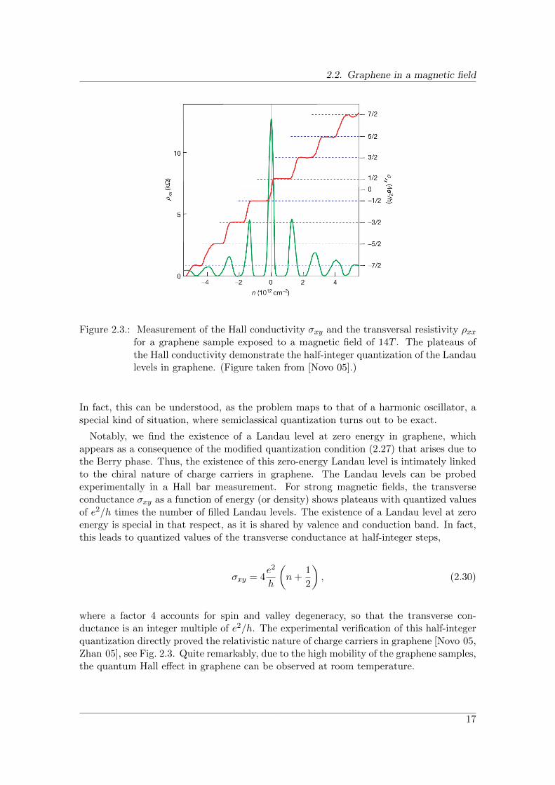
Figure 2.3.: Measurement of the Hall conductivity σxy and the transversal resistivity ρxxfor a graphene sample exposed to a magnetic field of 14T . The plateaus ofthe Hall conductivity demonstrate the half-integer quantization of the Landaulevels in graphene. (Figure taken from [Novo 05].)
In fact, this can be understood, as the problem maps to that of a harmonic oscillator, aspecial kind of situation, where semiclassical quantization turns out to be exact.
Notably, we find the existence of a Landau level at zero energy in graphene, whichappears as a consequence of the modified quantization condition (2.27) that arises due tothe Berry phase. Thus, the existence of this zero-energy Landau level is intimately linkedto the chiral nature of charge carriers in graphene. The Landau levels can be probedexperimentally in a Hall bar measurement. For strong magnetic fields, the transverseconductance σxy as a function of energy (or density) shows plateaus with quantized valuesof e2/h times the number of filled Landau levels. The existence of a Landau level at zeroenergy is special in that respect, as it is shared by valence and conduction band. In fact,this leads to quantized values of the transverse conductance at half-integer steps,
σxy = 4e2
h
(n+
1
2
), (2.30)
where a factor 4 accounts for spin and valley degeneracy, so that the transverse con-ductance is an integer multiple of e2/h. The experimental verification of this half-integerquantization directly proved the relativistic nature of charge carriers in graphene [Novo 05,Zhan 05], see Fig. 2.3. Quite remarkably, due to the high mobility of the graphene samples,the quantum Hall effect in graphene can be observed at room temperature.
17

2. Electronic properties of graphene
Figure 2.4.: Left: Schematic picture of a Dirac particle moving in a rectangular potentialRight: Perfect transmission at normal incidence: The plot shows the Diracspectrum for ky = 0, which consists of two branches for right- and leftmovingstates (red and blue). The dotted line indicates the Fermi level. Black arrowsindicate the direction of the pseudospin, which points parallel (antiparallel) tothe momentum in the conduction (valence band). The spinor of a rightmovingelectron matches perfect the spinor of a rightmoving hole, so the electron isperfectly transmitted through the hole-doped region.
2.3. Klein tunneling
A striking manifestation of the wavenature of quantum particles is the effect, that quan-tum particles can penetrate classical forbidden areas, known as quantum tunneling. Thetransmission probability for this process decays exponentially with increasing height V0
of the potential barrier. In 1929, Oskar Klein studied quantum tunneling for relativis-tic particles, and surprisingly found that the tunneling probability becomes large again,once the potential height exceeds the electron’s rest mass, V0 > 2mc2. This at first sightcounterintuitive seeming effect can be explained with the fact that the Dirac equationallows for solutions at negative energies. Thus, while the barrier constitutes a forbiddenregion for positive energy states (electrons), it allows for the existence of negative energystates (positrons). Although Klein tunneling is a striking feature of relativistic quantumelectrodynamic, it is of little practicle relevance for electrons, as the preparation of suchpotential step requires gigantic electric fields. Relativistic quantum tunneling however hasimportant consequences for the electronic properties of graphene.
We now discuss scattering processes in graphene in a rectangular potential barrier, wherewe follow [Cast 09]. To be specific, we consider a potential barrier of height V0 present inthe strip 0 < x < L. The incident particle has energy E and approaches the barrier fromthe left under the angle φ. In the region I, left from the barrier, the wavefunction can bewritten as a sum of incident and reflected plane wave (see Eq. (2.9))
ψI(r) =1√2
(1seiφ
)ei(kxx+kyy) + r
1√2
(1
sei(π−φ)
)ei(−kxx+kyy) (2.31)
where s = sgn(E), kF = E/s~v, kx = kF cosφ, and ky = kF sinφ. For the reflected part(which contains the coefficient r), we note that the barrier inverts kx but conserves ky,such that the propagation angle becomes φr = π − φ.
18

2.3. Klein tunneling
In the barrier region (II), the wavefunction is of the form
ψII(r) = a1√2
(1
s′eiφ′
)ei(k
′xx+kyy) + b
1√2
(1
s′ei(π−φ′)
)ei(−k
′xx+kyy) (2.32)
with s′ = sgn(E−V0). Again, the barrier does not alter the y-component of the momentum– the x-component is then fixed by the dispersion,
E − V0 = s′~v√k′x
2 + k2y, (2.33)
and the angle of propagation is given by φ′ = arctan ky/k′x. (We assume here, that the
parameters are tuned in such a way, that the incident state can propagate through thebarrier, i.e. Eq. (2.33) can be solved for real k′x. The opposite case will be discussed lateron).
Finally, in the region right of the barrier (III), the wavefunction reads
ψIII(r) = t1√2
(1seiφ
)ei(kxx+kyy). (2.34)
The four coefficients r, a, b, t need to be determined from matching conditions. As theDirac equation is linear in the momentum operator, the wavefunction needs to be contin-uous at the potential steps at x = 0 and x = L, but no restriction on the derivative of thewavefunction is imposed (unlike for non-relativistic particles with parabolic dispersion).However, as we have to match both components of the spinor at the interfaces, we obtainfour equations that determine all the coefficients. We are interested in the transmission,which is found to be [Cast 09]
T = |t|2 =cos2 φ′ cos2 φ
cos2 k′xL cos2 φ′ cos2 φ+ sin2 k′xL(1− ss′ sinφ sinφ′)2. (2.35)
We note, that k′x also has a dependence on the angle φ. The angle-dependence of thetransmission is illustrated in Fig. 2.5
We now investigate, for which parameters the barrier becomes fully transparent, i.e.T = 1. We see, that this is the case, whenever k′xL = nπ, with integer n. This conditionprecisely accounts for resonant scattering, as the phase that a particle accumulates, whileit traverses the barrier forth and back, is a multiple of 2π. Such resonant scattering is well-known also from non-relativistic scattering processes. On the other hand, we find perfecttransmission also for normal incidence (φ = φ′ = 0) independent of length and height ofthe potential barrier. Such effect is in striking contrast to what one is experienced fromnon-relativistic scattering processes. Indeed, the perfect transmission at normal incidenceis a direct consequence of the chiral nature of charge carriers: Incident and reflected wavehave opposite pseudospin for normal incidence; the potential barrier however conservesspin, hence no particle can be reflected. We remark, that this effect holds true even ifthe charge carriers in the barrier are of hole-type, while they are of electron-type outsidethe barrier. In this case, a normally incident electron is propagating as a hole within thebarrier with 100 % efficiency, see also Fig. 2.4
19

2. Electronic properties of graphene
Figure 2.5.: Transmission T of the rectangular barrier as a function of the incident angle φ.Left: Rectangular barrier is hole-doped while the outside regions are electron-doped, with the same carrier concentration (V0 = 2E). Perfect transmission isobserved at normal incidence, and – depending on the parameters – at certainfinite angles, the latter corresponding to resonant tunneling (blue solid curve:kFL = 1, red dashed curve: kFL = 5). Right: Barrier is tuned to the Diracpoint (V0 = E). Perfect transmission is always observed at normal incidence,but the transmission rapidly goes to zero away from normal incidence, as thelength of the barrier is increased (blue solid curve: kFL = 1, red dashed curve:kFL = 2, green dotted curve: kFL = 10).
For the discussion sofar, we assumed a situation where the incident state can propagatethrough the barrier. Now we also want to illustrate the opposite case. For simplicity, weconsider the extreme case V0 = E, which tunes the barrier region at the Dirac point. Then,Eq. (2.33) allows for propagating states (real k′x) only for normal incidence. Otherwise,the dispersion relation can only be satisfied for imaginary k′x = ±iky. The states in thebarrier region are hence evanescent waves, ψ±(r) = χ±e
±kyx+ikyy, where the spinors χ±are determined by the Dirac equation at zero energy, σ ·∇ψ±(r) = 0. We then find, thatthe wavefunction in the barrier region is
ψII(r) = a
(10
)e(kyx+ikyy) + b
(01
)e(−kyx+ikyy). (2.36)
We then obtain for the transmission through the barrier
T =2 cos2 φ
cos 2φ+ cosh 2kyL=
2 cos2 φ
cos 2φ+ cosh (2kFL sinφ). (2.37)
Again, we find perfect transmission at normal incidence, as a consequence of the chiral-ity of the charge carriers. The transmission however quickly drops to zero away fromperpendicular incidence for long barriers, see Fig. 2.5.
2.4. Transport in clean graphene
Finally, we also want to study electric transport in clean graphene. To this end, we firstintroduce the Landauer-Buttiker formalism and then apply it to transport in graphene.
20

2.4. Transport in clean graphene
2.4.1. Landauer-Buttiker formalism
Transport in mesoscopic system is successfully described with the Landauer-Buttiker for-malism. We consider a sample that is connected to two electron reservoirs, denoted left(L) and right (R). The Landauer formula links the conductance of the sample to its scat-tering matrix, more precisely to the information how well the sample allows for electronsto be transmitted from one lead to the other. We here briefly sketch the main ideas of theLandauer formula und refer to the literature for a detailed derivation (e.g. [Datt 95]).
We first consider the case of a perfect one-dimensional conductor. Left and right leadare kept at different chemical potentials, µL and µR. The occupation probability for theelectrons of the lead to be in a state at a certain energy is given by the Fermi-Diracdistribution, which reads at zero temperature
fi(ε) =
1, ε < µi
0, ε > µi, (2.38)
for i = L,R. For a perfect conductor, where electrons are not backscattered, all right-moving (left-moving) electrons in the conductor originate from the left (right) lead, con-stituting a current
I =
∫ ∞0
dk
2πevkfL(εk) +
∫ 0
−∞
dk
2πevkfR(εk), (2.39)
where k labels the wavenumber of the one-dimensional quantum states, and εk and vk isthe associated velocity. Upon using vk = 1
~dεkdk , we rewrite this expression as
I = e
∫dε
2π~[fL(ε)− fR(ε)] =
e
h(µL − µR), (2.40)
where we made use of the xplicit distribution function Eq. (2.38). With the definition ofthe voltage V = (µL − µR)/e, we find for the conductance of a perfect one-dimensionalconductor G0 = I/V ,
G0 =e2
h, (2.41)
which we refer to as “conductance quantum” and whose reciprocal value corresponds toa resistance of 25.8 kΩ. We note that the conductance for the perfect one-dimensionalconductor results from the net charge transport of electrons impringing from left and rightlead. When the conductor is not perfect, electrons might be scattered back to the leads.It is then only the fraction T of electrons transmitted from on lead to the other, thatcontributes to the current
G =e2
hT. (2.42)
While the discussion so far applied for a strictly one-dimensional systems, it may beeasily generalized to higher dimensions, where the states in the leads are characterizedby an additional quantum number n resulting from the wavefunction for the transversecoordinates. These transverse degrees of freedom are also referred to as modes or channels,
21

2. Electronic properties of graphene
and for the Landauer conductance, one needs to sum the transmission from all the channelsin the left lead to all the channels in the right lead,
G =e2
h
∑nm
|tnm|2 =e2
hTr(tt†). (2.43)
Here tnm is the transmission amplitude for a particle starting from mode m in the leftlead to end up in the mode n in the right lead, while t denotes the corresponding matrix.
2.4.2. Conductance of a clean graphene sample
With the help of the Landauer-Buttiker formalism, we are now in the position to calculatethe conductance of a clean graphene sheet, following the calculation presented in [Twor 06].Our setup consists of a rectangular graphene sample of dimensions L ×W , which is incontact to metallic leads at x = 0 and x = L, which strongly dope the graphene regionunder it. The Hamiltonian reads
H = vp · σ + V (x) (2.44)
where V (x) models the potential induced by the leads
V (x) =
VL, x < 0 or x > L
0, 0 < x < L(2.45)
In principle, electronic transport in graphene nanonibbons can be very sensitive to theboundary conditions, i.e. if the edges are of armchair or zigzag type. We here avoidthese issues by considering a very wide sample W L, so that boundary effects do notinfluence the value of the conductance. We then can choose periodic boundary conditions,for which the calculation is most simple: As the system is translationally invariant in they-direction, the wavefunctions are of the form
Ψn(x, y) = ψn(x)1√Weiqny (2.46)
with the quantized transverse momenta
qn = n2π
W(2.47)
where n is an integer number. We then solve the Dirac equation for each transverse modein each of the three regions left lead (L), central region (C) and right lead (R). For thescattering state of a particle impringing from the left lead, we write
ψ(L)n (x) = χn,kLe
ikLx + rnχn,−kLe−ikLx
ψ(C)n (x) = αnχn,−ke
ikx + βnχn,−ke−ikx
ψ(R)n (x) = tnχn,kLe
ikLx, (2.48)
22

2.4. Transport in clean graphene
with coefficients rn, tn, αn, βn Here, the wavenumbers k and kL are found from the rela-tivistic dispersion
k =√
(ε/~v)2 − q2n (2.49)
kL =
√(ε− VL
~v
)2
− q2n, (2.50)
where ε denotes the energy of the electrons in graphene. The wavenumber k in the samplemay be real or imaginary, discriminating oscillatory and evanescent modes. In the leads,we only account for propagating modes. The spinor structure of the solution reads
χn,k =1√2
(1
szn,k
), zn,k =
k + iqn√k2 + q2
n
(2.51)
where s = ± refers to conduction/valence band. This expression for the spinor is valid forboth real and imaginary k. For real k, we have zn,k = eiθ, where θ is the polar angle of thewavevector (k, qn), which gives the well-known expression from Eq. (2.9). We consider thelimit of highly doped leads, VL → −∞, so that the spinors in the leads have a particularsimple form
χn,±kL =1√2
(1±1
). (2.52)
We can easily interpret these results, as for fixed qn and VL → −∞ the electrons aremainly moving in the x-direction in the leads, and thus the spinors are eigenstates of theσx Pauli matrix.
The next step is to connect the wavefunctions at the lead-sample interfaces x = 0 andx = L. As discussed in the previous Section, we demand the wavefunction to be continuousat the interfaces, but we pose no restriction on the derivative. One then obtains for thetransmission
Tn = |tn|2 =
∣∣∣∣∣ k
k cos kL+ i√k2 + q2
n sin kL
∣∣∣∣∣2
. (2.53)
Having determined the transmission for each channel, we can calculate the Landauerconductance
G = 4e2
h
∑n
Tn, (2.54)
where a factor 4 accounts for the spin and valley degeneracy in graphene. In the short-and-wide limit W L, the summation over transverse momenta can be replaced by anintegration ∑
n
→ W
2π
∫dq (2.55)
The conductance for a short-and-wide sample as a function of energy is shown in Fig.2.6. If we tune the energy of the charge carriers in the sample to zero, transport is mediatedby evanescent modes,
Tn =1
cosh2 qnL. (2.56)
23

2. Electronic properties of graphene
Figure 2.6.: Conductance of an undoped graphene sheet, as a function of energy.
Nevertheless, the conductivity acquires a finite value,
G =4
π
e2
h
W
L⇔ σ =
4
π
e2
h. (2.57)
As one increases the energy in the sample, more and more modes can propagate throughthe sample, and the conductance increases roughly linear with energy.
24

3. Resonant scattering in graphene with agate-defined chaotic quantum dot
The successful production of high-quality nanoflakes together with the strictly two-dimen-sional nature of the material have made graphene to a promising candidate for futurenanoelectronic devices. Of particular interest is the realization of quantum dots, whereelectrons are confined locally in a narrow region of the graphene sample. A well-establishedexperimental route in the fabrication of quantum dots utilizes metallic gates nearby thesample, that repel electrons from regions outside the quantum dot. Such procedure how-ever is problematic for graphene, in view of the Klein tunneling, that allows the electronsto escape the quantum dot, as we discussed in the previous chapter.
Recently, Bardarson, Titov and Brouwer argued that there is an exception to this state-ment, and for geometries, for which the Dirac equation is separable, confinement with thehelp of metal gates should be possible [Bard 09]. Their study was supplemented by a nu-merical simulation of transport, where the graphene sheet containing the quantum dot, isattached to source and drain contacts. The interesting limit, where the dot is only weaklycoupled to the leads, was however not accessible with the applied numerical method. Thepurpose of this chapter is to study the geometry-dependence of gate-defined quantum dotsin graphene, where we gain new insights by applying a recently developed method fromRef. [Tito 10].
This chapter is structured as follows: After an introduction, we briefly summarize themain findings of [Bard 09] in Section 3.2. In Section 3.3, we then explain how the methodof [Tito 10] can be used to study gate-defined quantum dots of arbitrary geometries ingraphene. Our results are presented in Section 3.4. We conclude in section 3.5. The Secs.3.1, 3.3 – 3.5 of this chapter are based on the publication [Schn 11].
3.1. Introduction
There are two commonly used routes in the fabrication of quantum dots, which create aspatial confinement of the electrons. One way is to mechanically carve out nanostructures(“etched quantum dots”). The other possibility relies on metallic gates, which can createforbidden regions for the electrons, when the Fermi level is shifted in the bandgap of thenanosystem. Due to the absence of a bandgap in graphene, experimentalists pursue thefirst possibility for the fabrication of graphene quantum dots [Bunc 05, Pono 08, Stam 08,Schn 09, Gutt 12, Jaco 12].
In a recent article [Bard 09], Bardarson, Titov and Brouwer showed that the commonassertion, that it is not possible to confine electrons in graphene with metal gates, canbe circumvented in certain cases. In their article, they considered a quantum dot that issurrounded by undoped graphene. As the density of states vanishes, when the Fermi level
25

3. Resonant scattering in graphene with a gate-defined chaotic quantum dot
is tuned to the Dirac point, such scenario comes closest to the “formation of a bandgap”in graphene. We learned in the previous chapter, that Klein tunneling opens a way topenetrate the surrounding. However, Klein tunneling is only effective when the electronhits the surface of the quantum dot at perpendicular incidence, while the transmissionprobability quickly drops to zero away from perpendicular incidence. The authors ofRef. [Bard 09] therefore argued, that confinement should be possible in graphene, whenthe geometry is such, that the Dirac equation is separable, and the associated classicalmotion is integrable. An example for such a geometry is a disc-shaped dot with a uniformpotential inside the disc. Generic classical trajectories in this geometry will never hit thesurface at perpendicular incidence, which renders Klein tunneling ineffective. On the otherhand, in a geometry with classical chaotic dynamics, every electron eventually the surfaceat perpendicular incidence, and the quantum dot lacks confinement (see also Fig. 1.1 ofChapter 1).
To further investigate this reasoning based on classical arguments, the authors of Ref.[Bard 09] numerically simulated the two-terminal transport, when the quantum dot sur-rounded by undoped graphene is attached to source and drain contacts, see Fig. 3.1.Bound states of the quantum dot are then revealed as resonances in the two-terminalconductance. For a circular geometry, the authors indeed found a series of sharp reso-nances, corresponding to well-confined quantum states, while for a stadium geometry, theresonances are typically broader, indicating a lack of confinement. The difference betweenintegrable quantum dots and non-integrable quantum dots becomes most pronounced inthe limit that the distance L between the two metallic contacts becomes large, in compar-ison to the size of the quantum dot. However, a detailed investigation of this limit wasnot possible in Ref. [Bard 09] because of limitations of the numerical approach requiredto study the non-integrable case.
In the mean time, the problem of gate-defined quantum dots in graphene has beenrevisited by Titov, Ostrovsky, Gornyi, Schuessler, and Mirlin [Tito 10]. These authorsadapted the matrix Green function method, originally developed by Nazarov in the contextof mesoscopic superconductivity [Naza 94], to two-terminal transport in graphene. Oneof their main results is a relation between the two-terminal conductance of a rectangulargraphene sheet containing an arbitrary “scatterer” and the scatterer’s T -matrix. A gate-defined quantum dot is a special case of such a scatterer. Using this method, Titov etal. were able to give an analytic expression for the conductance of an otherwise undopedgraphene sheet with a disc-shaped quantum dot, reproducing the numerically obtainedconductance of Bardarson et al. [Bard 09].
In this chapter, we want to find out what information the matrix Green function methodmakes available if we consider undoped graphene with a non-separable quantum dot. Thisrequires a numerical calculation of the T matrix, since no analytical results are availablefor a quantum dot for which the Dirac equation is not separable. We here show that thenumerical evaluation of the T matrix can be done very efficiently and that the remainingsteps in the matrix Green function formalism can still be carried out analytically. Inparticular, once the T matrix of the quantum dot is known, the L dependence of theconductance resonances can be found without additional numerical effort. This allows usto obtain information about the constitution of the resonances deep into the regime inwhich resonances are separated, which could not be addressed with the generic numerical
26

3.2. Electrostatic confinement in a gate-defined graphene quantum dot
Figure 3.1.: Geometry of the two-terminal transport setup: A rectangular sample ofgraphene of dimensions L×W , that contains a quantum dot of size R.
algorithm used in Ref. [Bard 09]. We apply the formalism to a stadium-shaped quantumdot. Our main result is that the resonance lineshapes are described by the Fano resonanceformula in the case of the stadium-shaped (i.e., non-separable) quantum dot, while theyare Breit-Wigner resonances for the disc-shaped dot.
3.2. Electrostatic confinement in a gate-defined graphenequantum dot
Before we enter the presentation of our results, we give a brief summary of the mainfindings of Ref. [Bard 09], in order to keep the thesis self-contained.
3.2.1. Bound states of a circular quantum dot
We start by considering a circular quantum dot in a graphene sheet. For this situation,an analytic calculation of the resonant levels is possible. We thus study the Hamiltonian
H = vp · σ + V (r), (3.1)
where the gate potential V (r) accounts for the circular quantum dot of radius R,
V (r) =
−~vV0, r < R
0, r > R,(3.2)
The constant V0 has the dimension of inverse length and we choose V0 > 0, so that thequantum dot is electron doped. Although the potential V (r) is steplike in our description,
27

3. Resonant scattering in graphene with a gate-defined chaotic quantum dot
we remark, that this step is required to be smooth on the scale of the lattice constant, sothat a description in terms of a single Dirac point is justified.
The radial symmetry of the problem facilitates a solution in polar coordinates (r, θ), forwhich the kinetic part of the Hamiltonian is found to be
vp · σ = −i~v(
0 ∂−∂+ 0
), (3.3)
with the operators
∂± = e±iθ(∂r ±
i
r∂θ
). (3.4)
The radial symmetry furthermore suggests to look for common eigenstates of the Hamilto-nian and the angular momentum operator. As the kinetic part strongly couples orbital andpseudospin degrees of freedom, neither orbital angular momentum, nor pseudospin aloneis conserved. What is conserved however, is the total angular momentum jz = lz + ~
2σz.We therefore seek for eigenstates of the form
ψm(r) = eimθ
(e−i
θ2ϕm,+(r)
eiθ2ϕm,−(r)
)(3.5)
which are eigenstates of the total angular momentum jzψm = m~ψm, with half-integerquantum number m.
Inside the dot, for r < R, the Dirac equation yields the following coupled equations forthe radial wave functions ϕm,±,(
∂r − (m− 12)1r
)ϕm,+(r) = iV0ϕm,−(r),(
∂r + (m+ 12)1r
)ϕm,−(r) = iV0ϕm,+(r). (3.6)
The solution of these equations read
ϕm,+(r) = J|m−1/2|(V0r)
ϕm,−(r) = isgn(m)J|m+1/2|(V0r), (3.7)
where Jn(x) is the Bessel function of n-th order. We here required the solution to beregular at the origin.
Outside the dot, the gate potential is zero, and the equations for ϕm,± decouple. Here,the radial wave functions behave as a power law
ϕm,+(r) = a+rm−1/2, ϕm,−(r) = a−r
−m−1/2, (3.8)
with coefficients a±. We require that the wave function must not diverge for r → ∞,which gives the constraint a+ = 0 (m > 0) or a− = 0 (m < 0). From continuity of thewavefunction at r = R, we then obtain the resonance condition
J|m|−1/2(V0R) = 0, (3.9)
28

3.3. Model and method
i.e. we expect resonances, when the parameter V0R is tuned to be a root of a Besselfunction. Outside the dot, one component of the spinor wavefunction is zero, while theother is decaying as
ψ ∝ r−(|m|+1/2). (3.10)
Interestingly, for |m| = 1/2 we find a marginally non-normalizable state.To sum up, the bound states of a disc-shaped quantum dot have been calculated, which
are classified by their angular momentum. We know at which parameters resonances areexpected, and how the wavefunction of a resonant state is decaying outside the dot.
3.2.2. Resonances in a two-terminal conductance setup
For the further studies, Bardarson et al. investigated numerically two-terminal transportof a quantum dot surrounded by undoped graphene and attached to source and draincontacts. In Fig. 3.2, we display their results for the conductance as a function of thedot’s gate voltage, for a circular quantum dot, an example for a classical regular structure,and a stadium quantum dot, a prototypical example for a classical chaotic geometry. Theanalysis of the conductance can be used to detect the bound states of the quantum dot,which show up as resonant features.
For the circular quantum dot of size R, one finds that the position of the resonances inthe conductance agree with roots of the integer Bessel functions, in line with the theoreticalprediction, Eq. (3.9). The resonances have a definite angular momentum. Their finite
width Γ can be estimated as Γ ∼ |ψ(L)|2L|ψ(R)|2R , where ψ denotes the wavefunction outside the
dot, Eq. (3.10), and L is the distance between the leads. From this estimate, we conclude,that the width of the resonances scales as
Γ ∝ (R/L)2|m|. (3.11)
Such behaviour was confirmed by the studies of [Bard 09] (data not shown here). Reso-nances belonging to the lowest possible angular momentum, |m| = 1
2 , gives rise to broadresonances, Γ ∝ (R/L), while bound states from higher angular momenta give rise to muchsharper resonances. The figures also show, that the resonances for the chaotic structureare typically much broader than for the regular structure, indicating a weaker confinement.For the specific parameters of the simulation in Ref. [Bard 09] however, the resonances arestill overlapping. Due to numerical limitations, it was not possible to access the regimeof well-seperated resonances and to carry out a detailed study of the resonances of thechaotic dot. This task will be completed in the remaining part of this chapter.
3.3. Model and method
We now describe, how to utilize the matrix Green function formalism in order to studytransport in graphene with a gate-defined quantum dot. In addition to the calculationof the bound states of the circular dot in the previous section, our system is attached tosource and drain contacts. The setup thus consists of a rectangular sample of graphene oflength L and width W L, described by the Hamiltonian
H = −i~vσ ·∇ + U(x) + V (r). (3.12)
29

3. Resonant scattering in graphene with a gate-defined chaotic quantum dot
Figure 3.2.: Two-terminal conductance of an undoped graphene sheet containing an elec-trostatically gated region (quantum dot). Upper panel: Circular quantumdot; positions of the resonances agree with the theoretical prediction (indi-cated with arrows, parameters: R/L = 0.2, W/L = 6). Lower panel: Stadiumquantum dot (parameters: R/L = 0.2,W/L = 6, 2a/R =
√3.) [Figures
adopted from [Bard 09].]
The potential V (r) defines the quantum dot. It takes a constant value V (r) = −~vV0
inside the quantum dot, and V (r) = 0 outside the dot. The potential U(x) accounts forthe metallic leads and is set to be U(x)→ −∞ for x < 0 and x > L, whereas U(x) = 0 for0 < x < L, so that the graphene sheet is tuned to the Dirac point in the region of interest.
In order to calculate the two-terminal conductance of the system, we apply Nazarov’smatrix Green function formalism [Naza 94], which has been adapted to graphene by Titovet al. [Tito 10]. Below, we summarize the essential elements of this method. Centralobject is a 4× 4 matrix Green function G with matrix structure in the pseudospin space[corresponding to the Pauli matrices σx and σy in the Dirac equation (3.12)] and the“retarded-advanced” (RA) space. The matrix Green function is defined by the equation(
ε−H + i0 −~vσxζδ(x)−~vσxζδ(x− L) ε−H − i0
)G(r, r′) = δ(r− r′), (3.13)
where ε is the quasiparticle energy (set to zero in the remainder of the calculation), and
30

3.3. Model and method
ζ is an additional parameter. Following Ref. [Tito 10], we define the generating functionF(φ) as
F(φ) = Tr ln G−1∣∣ζ=sin(φ/2)
, (3.14)
where the trace operation includes summation over RA and pseudospin indices, as wellas integration over spatial coordinates. The generating function F contains informationabout the full counting statistics of two-terminal transport through the system [Naza 94].Here, we restrict our discussion to the two-terminal conductance G, which is obtainedfrom F through the equality
G = −2g0∂2F∂φ2
∣∣∣∣φ=0
, (3.15)
where g0 = 4e2/h is the conductance quantum in graphene.Denoting the matrix Green function for the graphene sheet without quantum dot (V =
0) as G0, and writing F0 = Tr ln G−10 , we rewrite Eq. (3.13) as
δF = F − F0
= Tr ln(1− V G0). (3.16)
The matrix Green function G0 for the clean system (without dot) has been calculatedanalytically in Ref. [Tito 10]. The explicit expression is rather lengthy and can be foundin Appendix A.1. Substituting the explicit expression for G0 into Equation (3.15) thengives
G =g0W
πL+ δG, δG = −2g0
∂2δF∂φ2
∣∣∣∣φ=0
, (3.17)
where the first term corresponds to the conductivity of clean graphene [Ludw 94, Zieg 98,Pere 06, Twor 06] and the second term gives the correction from the presence of thequantum dot, which is the focus of our calculation.
The calculation of Ref. [Tito 10] proceeds by expressing δF in terms of the T matrix ofthe quantum dot. Hereto, one introduces the Green function g for zero-energy quasipar-ticles in an infinite sample (i.e., with V = U = 0),
g(r, r′) = − i
2π~vσ · (r− r′)
|r− r′|2, (3.18)
as well as the functionGreg = G0 − g, (3.19)
which, being a difference of two Green functions, is regular if the spatial arguments coin-cide. With the standard Born series for the T matrix [Mess 61],
T = (1− V g)−1V, (3.20)
one finds [Tito 10]δF = Tr ln(1− TGreg), (3.21)
up to terms that do not depend on the counting field φ. Equation (3.21) is the basis forour further investigations.
31

3. Resonant scattering in graphene with a gate-defined chaotic quantum dot
We will consider the limit that the size of the quantum dot is small in comparison tothe length L. In that case, it is advantageous to expand Greg around the position r0 ofthe center of the quantum dot. After a short algebraic manipulation, which is carried outin Appendix A.1, one finds that one may replace the operators T and Greg in Eq. (3.21)by matrices with elements Tµν and Gµνreg, with µ, ν = 0, 1, 2, . . . and
Gµνreg =∂µ
∂xµ∂ν
∂x′νGreg(r, r′)
∣∣∣∣r=r′=r0
, (3.22)
Tµν =1
µ!ν!
∫d2rd2r′[(x− x0)− iσz(y − y0)]µ
×T (r, r′)[(x′ − x0) + iσz(y′ − y0)]ν . (3.23)
Note that each element Gµνreg is a 4 × 4-matrix with non-trivial operation on pseudospinand RA degrees of freedom, whereas Tµν acts in pseudospin space only and leaves the RAspace untouched. With this replacement, the trace in Eq. (3.21) is taken over the matrixindices µ or ν, the pseudospin degrees of freedom, and the RA degrees of freedom.
Essentially, the matrix Tµν is the T matrix in a partial-wave expansion. In graphene,the partial wave expansion involves waves of angular momentum σ(µ+ 1/2), with σ = ±1a pseudospin index and µ = 0, 1, 2, . . . the index of the matrix Tµν . The correspondingbasis functions ψk,µ,σ(r) are defined at a finite energy ε = ~vk only, where, for definiteness,we choose k > 0. They are the solutions of the Dirac equation Hψk,µ,σ(r) = εψk,µ,σ(r) inthe absence of the potentials U and V . With the matrix notation Ψkµ = (ψk,µ,+1, ψk,µ,−1),one has
Ψkµ(r) =
√k
4π
(eiµθJµ(kr) ie−i(µ+1)θJµ+1(kr)
iei(µ+1)θJµ+1(kr) e−iµθJµ(kr)
), (3.24)
where Jν is a Bessel function and we used polar coordinates (r, θ). Denoting the T matrixin the partial-wave basis by Tµν(k), one then finds that
Tµν = limk→0
2µ+ν+2π
kµ+ν+1Tµν(k), (3.25)
where we again refer to appendix A.1 for details. In our discussion below, we will refer tothe mode indices µ, ν = 0, 1, 2, . . . as s, p, d, . . . .
It remains to describe a method to calculate the T -matrix Tµν(k) for a specific quantumdot potential V (r). This is done through by first relating T to the scattering matrix Sµν(k)in the partial-wave basis,
Sµν(k) = δµν − 2πiTµν(k). (3.26)
The scattering matrix Sµν(k) relates the coefficients of incoming (−) and outgoing (+)parts of the basis functions (3.24) at energy ε = ~vk. Again using the shorthand notation
Ψ(±)kµ = (ψ
(±)k,µ,+1, ψ
(±)k,µ,−1), these are
Ψ(±)kµ (r) =
√k
4π
(eiµθH
(±)µ (kr) ie−i(µ+1)θH
(±)µ+1(kr)
iei(µ+1)θH(±)µ+1(kr) e−iµθH
(±)µ (kr)
), (3.27)
32

3.3. Model and method
where the H(±)µ = Jµ ± iYµ are Hankel functions of the first (+) and second kind (−),
respectively. The scattering matrix Sµν(k) is then defined through the asymptotic form ofthe solution of the Dirac equation Hψk(r) = ~vkψk(r) for r →∞, which takes the generalform
ψk(r) =∑µ
(Ψ
(+)kµ (r)akµ + Ψ
(−)kµ (r)bkµ
), (3.28)
with, in 2× 2 matrix notation,
akµ =∑ν
Sµν(k)bkν . (3.29)
To find Sµν(k), we employ a variation of a method commonly applied to rectangularstrips of disordered graphene [Bard 07]. Hereto, we divide the graphene sheet in circularslices aj−1 < r < aj , j = 1, . . . , N , with a0 = 0 and aN so large that V (r) = 0 for r > aN .We then obtain the scattering matrix S(k) by solving two auxiliary scattering problemsfirst.
In the first auxiliary problem, we set the potential V to zero everywhere, except in thecircular slice aj−1 < r < aj . In this case, the wavefunctions can be expanded in incomingand outgoing partial waves for r < aj−1 as well as for r > aj . The general solution of theDirac equation in the regions r < aj−1 and r > aj can be characterized by means of tworeflection matrices ρj and ρ′j and two transmission matrices τj and τ ′j , such that ρ relatesthe coefficients of outgoing partial waves on the exterior to the coefficients of incomingpartial waves on the exterior etc. If δa = aj − aj−1 is sufficiently small, these matricescan be calculated in the first-order Born approximation. Writing ρµν = δρµν , ρ′µν = δρ′µν ,τµν = δµν + δτµν , and τ ′µν = δµν + δτ ′µν , this calculation gives
δρµν = − iπ
2~v
∫aj−1<r<aj
drΨ(+)kµ (r)†U(r)Ψ
(−)kν (r),
δτµν = − iπ
2~v
∫aj−1<r<aj
drΨ(−)kµ (r)†U(r)Ψ
(−)kν (r),
δρ′µν = − iπ
2~v
∫aj−1<r<aj
drΨ(−)kµ (r)†U(r)Ψ
(+)kν (r),
δτ ′µν = − iπ
2~v
∫aj−1<r<aj
drΨ(+)kµ (r)†U(r)Ψ
(+)kν (r),
up to corrections of higher order in δa.In the second auxiliary problem, we set V to zero for r > aj only. Defining Sj(k) to be
the scattering matrix for this situation, we obtain the recursion relation
Sj(k) = ρj + τ ′j(1− Sj−1(k)ρ′j)−1Sj−1(k)τj . (3.30)
Together with the initial condition S0 = 1 and the equality SN = S this leads to thedesired solution.
Unitarity implies the relations δρ′j = −δρ†j , δτj = −δτ †j , and δτ ′j = −δτ ′†j . Consistentwith the Born approximation, we may rewrite the recursion relation (3.30) as
Sj(k) = Sj−1(k)[1 + iδhj ], (3.31)
33

3. Resonant scattering in graphene with a gate-defined chaotic quantum dot
where
iδhj = S†j−1(k)δρj + δρ′jSj−1(k)
+ S†j−1(k)δτ ′jSj−1(k) + δτj (3.32)
is a hermitian matrix.Although this concludes our formal description of the method, there are a few issues
regarding the numerical implementation that we also need to discuss:(i) — For the final result, we have to take the low-k limit of the scattering matrix S(k),
which, at first sight, may be problematic because the Hankel functions appearing in theBorn approximation for the matrices δρ, δρ′, δτ , and δτ ′ diverge in this limit. However,this problem can easily be circumvented by shifting the potential V (r) → V (r) + ~vk′for r < aN , while at the same time increasing the quasiparticle energy according tok → k + k′. This means that we transfer contributions between the free propagationand the perturbation. We then solve the scattering problem inside the disc starting from“free” Dirac fermions with energy ~v(k + k′), which remains finite in the limit k → 0.The wavefunction outside the disc, where free electrons have momentum k, can be foundby matching to the wave function inside the disc, and contains the information of thescattering matrix we need.
For the low-k-expansion of the scattering matrix, we then find an expression of the form
Sµν(k) = δµν + S′µν(k′)kµ+ν+1 +O(kµ+ν+2), (3.33)
where S′(k′) depends on aN , k′, and the scattering matrix SN (k′) obtained for the modifiedproblem where we have replaced k by k′ + k and safely can take the limit k → 0. Adetailed derivation is given in Appendix A.2. Note, that the expansion in Eq. (3.33) givesus precisely that order in k, that we need in order to obtain the matrix Tµν in Eq. (3.25).
The wavenumber k′ of the quasiparticles can be chosen arbitrarily, and we have verifiedthat the result of our calculations do not depend on the choice of k′. However, onemay exploit this freedom for a wise choose of k′. It should be not too small, becauseotherwise the Hankel functions in the spherical incoming and outgoing waves become toolarge, indicating the fact that particles are repelled from the origin and therefore the Bornapproximation looses its applicability. On the other hand, if the wave vector k′ is chosentoo large, the effective potential V +~k′v gets large, too, and the thickness δa of the sliceshas to be decreased.
(ii) — It is sufficient to choose the radius a0 of the first slice such, that V (r) is uniformfor r < a0. For this situation an exact solution is available.
(iii) — In order to guarantee numerical stability during multiplication of scatteringmatrices, we change Eq. (3.31) to
Sj(k) = Sj−1(k)
(1 + i
δhj2
)(1− iδhj
2
)−1
, (3.34)
which is valid up to corrections beyond the accuracy of Born approximation, but ensuresthat the scattering matrices remain unitary at all times.
(iv) — In the calculation of the scattering matrix, we keep a total of M modes. Afterthe calculation of the full scattering matrix S, we then further truncate the scattering
34

3.4. Two-terminal conductance with stadium-shaped quantum dot
Figure 3.3.: Conductance versus gate voltage V0 for an undoped graphene sheet with agate-defined stadium-shaped quantum dot. The parameters of the numericalcalculation are 2a/R =
√3 and L/R = 5. The curves correspond to the
numerical calculation using the method of Sec. 3.3, with contributions to theT matrix up to d-wave (blue, solid), and to a direct numerical solution of theDirac equation (red, points; data taken from Ref. [Bard 09]).
matrix upon calculation of the determinant in Eq. (3.21), keeping matrix elements Sµν
with µ, ν = 0, 1, ...,M ′ only. Keeping a large number of modes M in the calculation ofthe scattering matrix is important in order to properly resolve the dynamics inside thequantum dot. The number of modes M ′ required for the calculation of the conductancedepends on the ratio of the size L of the graphene sheet and the size of the quantum dot,and can be kept small if this ratio is large. The numerical calculation of the conductancehas converged, when the result does no longer change upon increasing M , M ′ or N . Forthe results of the conductance shown here, we kept channels up to d-wave (M ′ = 2) only,which we found to be sufficient for the parameters chosen in our calculation.
3.4. Two-terminal conductance with stadium-shaped quantumdot
3.4.1. Two-terminal conductance
As a nontrivial application of the formalism laid out in the previous Section, we havecalculated the two-terminal conductance of a stadium-shaped quantum dot in an otherwiseundoped graphene steet. The quantum dot is placed halfway between the contacts. It ischaracterized by the radius R of the circular pieces and the length 2a of the linear segment.The gate voltage V (r) = −~vV0 for r inside the quantum dot, and V (r) = 0 otherwise. Inour calculations, we have included contributions up to d-wave in the T matrix, whereasas many modes were used for the calculation of the scattering matrix S as were necessaryto reach convergence. (See the discussion at the end of the previous section.)
In Fig. 3.3, we show the two-terminal conductance as a function of the gate voltage V0.The conductance exhibits several resonances due to the formation of quasi-bound states
35

3. Resonant scattering in graphene with a gate-defined chaotic quantum dot
in the stadium. The parameters for the data in this figure are chosen to be the same asin Ref. [Bard 09], so that the results can be compared. The excellent agreement betweenboth curves concerns the position as well as the shape of the resonances. We attributesmall deviations in the resonance heights to corrections from higher angular momentumthat were not taken into account in the calculations. Such corrections disappear uponincreasing the ratio of system size vs. dot size L/R (see discussion below).
The effect of inclusion of successive angular momentum channels in the T matrix (whilekeeping essentially all angular momentum channels in the calculation of the scatteringmatrix S) is illustrated in Fig. 3.4, where, in the upper panel, we show a close-up ofthe data of Fig. 3.3 with one, two, and three angular momentum channels included inthe final step of the calculation (i.e. with truncation at M ′ = 0, 1, 2). This figure clearlydemonstrates that each resonance has contributions from more than one angular mode,as is to be expected for a chaotic quantum dot. In particular, we find that all resonanceshave a non-vanishing s-wave contribution, so that the resonance position can be extractedfrom the s-wave channel solely. For the data shown in Fig. 3.3, one needs to include the p-wave contribution in order to obtain the correct resonance shape. The effect of the d-wavecontribution is small, which we find remarkable, because the ratio of dot size 2(R + a)versus contact size L is ≈ 0.75, which is not small in comparison to unity. The lower panelof Fig. 3.4 shows conductance data for M ′ = 0, 1, 2, showing that the convergence withrespect to M ′ quickly improves upon increasing L/R.
We conclude, that most information about the resonances that is relevant for transportat large or moderately large L/R is encoded in the contributions from small angularmomentum, and is therefore stored in a small set of parameters. That fact is a strongindication of the power of the method employed here, in comparison to a direct simulationof the Dirac equation.
3.4.2. Lineshape
The main advantage of the present method over the direct numerical solution of the Diracequation is that it allows one to extend the conductance calculations to the regime L R:The complete dependence on the length L is encoded on the Green function Greg, whichis known analytically. It is only in the regime L R that resonances are well separatedand can be characterized individually. The calculations of Ref. [Bard 09], on the otherhand, were limited to the regime L ≤ 5R, where resonances were still strongly overlapping.(Reference [Bard 09] also considered the case L ≈ 8R for W = L. However, in that casethe conductance is strongly influenced by the finite width W of the graphene sheet.)
In Fig. 3.5 we show how the first and second resonance behaves upon increasing thecontact size L at fixed dot size R. The plots illustrate that the resonance width shrinks,while the height saturates. The asymmetry of the line shape disappears in the limitL/R → ∞, consistent with the expectation that s-wave scattering dominates if L R.Similar behaviour is found for the other resonances.
In order to quantitatively analyze the lineshapes, we note that each resonance is char-acterized by a divergence of the T matrix. With a suitable parameterization of thesedivergencies an explicit expression for the resonance lineshape can be obtained. Heretowe introduce the dimensionless variable ε = V0R. Then, close to a divergence at ε0, the
36

3.4. Two-terminal conductance with stadium-shaped quantum dot
Figure 3.4.: First four conductance resonances: The conductance has been calculatedusing Eq. (3.21) with the T matrix truncated after the s-wave (blue, dashed),p-wave (red, dotted), and d-wave angular-momentum channel (green, solid),corresponding to M ′ = 0, 1, 2, respectively. In the upper panel, we set L/R =5, while in the lower panel, L/R = 10. The ratio a/R remains the same as inFig. 3.3.
divergent part of Tµν is of the form
Tµν(ε) ' Rµν
ε− ε0, (3.35)
where the matrix Rµν contains the information about the resonance shape. The matrixelements Rµν are related by hermiticity, Rµν = (Rνµ)† and time-reversal symmetry, Rµν =σy(R
νµ)Tσy. Moreover, for the specific problem we consider here, inversion symmetry andreflection symmetry impose further constraints on R, which allow us to parameterize thematrix as
R =
lsσ0 ilspσx lsdσ0
−ilspσx lpσ0 ilpdσxlsdσ0 −ilpdσx ldσ0
, (3.36)
where σ0 is the 2× 2 unit matrix. Due to Kramers degeneracy, R can be decomposed intotwo identical submatrices, which, for a generic resonance, are of unit rank. (In a chaoticquantum dot level repulsion ensures that this condition is always fulfilled.) This gives the
37

3. Resonant scattering in graphene with a gate-defined chaotic quantum dot
Figure 3.5.: Dependence of the first and second resonance on the ratio of dot size versussystem size R/L.
additional constraints
l2sp = lslp, l2sd = lsld, l2pd = lpld (3.37)
on the parameters in Eq. (3.36). Note, that ls , lp, and ld have the dimension of a length,length3, and length5, respectively.
Substituting Eq. (3.36) into Eq. (3.21) and making use of the condition (3.37), we findthat the line shapes are described by the Fano resonance formula [Fano 61]
G = Gnr|2(ε− ε0) + qΓ|2
4(ε− ε0)2 + Γ2(3.38)
Here, Gnr is the non-resonant conductance, Γ is the resonance width, ε0 is the resonanceposition, and q is the complex “Fano parameter”. After subtracting the backgroundconductance Gnr, we rewrite Eq. (3.38) as
δG = g0β + 4α(ε− ε0)
4(ε− ε0)2 + Γ2, (3.39)
where β = (Gnr/g0)(|q|2 − 1)Γ2 and α = (Gnr/g0)Re q. For α = 0 the resonance has aBreit-Wigner shape; Non-zero α is responsible for an asymmetry in the lineshape. When
38

3.4. Two-terminal conductance with stadium-shaped quantum dot
we express the resonance parameters through the entries of R, we also use σsp = sign(lsp)etc., which is not fixed by Eq. (3.37):
ε0 = ε0 +π√lslpσsp
24L2−
7π3√lpldσpd
960L4, (3.40)
Γ =
∣∣∣∣ ls2L+π2lp8L3
+π2√lsldσsd
4L3+
5π4ld32L5
∣∣∣∣ , (3.41)
β =2l2sπ2L2
+2lpls3L4
+8√l3s ldσsd3L4
+19l2pπ
2
72L6,
+481ldlsπ
2
180L6+
17lp√lsldσsdπ
2
18L6+
61ldlpπ4
90L8,
+251√lsl3dσsdπ
4
180L8+
13549l2dπ6
28800L10(3.42)
α = −2√lslpσsp
πL2+π√lpldσpd
2L4. (3.43)
Note, that the shift ε0− ε0 of the resonance position, as well as the asymmetry α is absent,if the resonance consists of a single angular momentum component only.
Now consider the situation, where we fix the product V0R of the gate voltage quantumdot and the quantum dot size — i.e., we look at a fixed resonance — and increase the lengthL of the graphene sheet. Then, as long as ls 6= 0, at sufficiently large L, the conductancewill be determined by its s-wave contribution, so that the resonance line shape reduces tothe Breit-Wigner form. In this limit, the height for δG approaches the constant universalvalue 8g0/π
2, and the width scales as Γ = ls/2L, as was found previously by Titov et al.[Tito 10].
3.4.3. Comparison Disc - Stadium
We now summarize the main qualitative difference in the conductance resonances forstadium-shaped quantum dots, which have been considered numerically here and in Ref.[Bard 09], and disc-shaped dots, which were considered analytically in Ref. [Tito 10] andnumerically in Ref. [Bard 09]. The main difference, which is illustrated in Fig. 3.4, is thatgeneric resonances for the stadium dot have contributions from more than one angularmomentum channel. This means that the resonance lineshape changes from a Fano shapefor moderate ratios L/R to a Breit-Wigner lineshape for large L/R, as seen in Fig. 3.5.In the limit L/R → ∞ of isolated resonances, the height of the conductance resonancestakes the universal value 8g0/π
2, whereas the width of all resonances scales proportionalto R/L. Though we considered a stadium-shaped dot only, we believe, that the featuresfound here are generic and shared by all chaotic dots.
This is to be contrasted to the situation of a circular quantum dot, where differentangular momentum channels do not mix, and the resonances are of pure type (s-wave,p-wave,. . . ). The resonance lineshape is always of Breit-Wigner form and approachesa constant height upon taking the limit L/R → ∞. The asymptotic resonance heightdepends on the angular momentum channel, with a height 8g0/π
2 for s-wave resonances
39

3. Resonant scattering in graphene with a gate-defined chaotic quantum dot
(l = 0) and . 2g0 for higher angular-momentum channels (l ≥ 1). The resonance widthdepends on the angular momentum channel, Γ ∝ (R/L)2l+1.
We close this comparison with a comment on the results of Ref. [Bard 09]. There itwas found that the resonance height of the chaotic dot goes to zero upon taking thelimit of large L/R. This observation referred to a setup with aspect ratio W/L = 1 andperiodic boundary conditions along the transverse direction. For aspect ratio W L,only the mode with zero transverse momentum substantially contributes to transport[Twor 06]. Therefore, s-wave scattering does not affect the conductance, resulting theobserved suppressed height of s-wave conductance resonances. We verified that the samephenomenon occurs in our calculations, by evaluating the regularized Green function Greg
for finite width. This explains, why the resonances in Ref. [Bard 09] completely disappearin the limit of large L/R, while in our investigation for aspect ratio W L the height ofthe resonances remains finite.
3.5. Conclusion
In this chapter, we investigated the resonances of the conductance of a graphene sheet witha chaotic quantum dot. Using a numerical implementation of the matrix Green functionmethod of Ref. [Tito 10], we were able to study the behaviour of the resonances in thelimit of well-separated resonances. This essential limit could not be reached in the originaltreatment of the problem [Bard 09].
As was proposed in Ref. [Bard 09], the resonances of the chaotic dot behave significantlydifferent compared to the case when the gated region is circular. While the circular geom-etry does not allow for mode mixing, so that all resonances are Breit-Wigner resonanceswith a well-defined angular momentum, in the stadium dot, due to its non-integrabledynamics, all resonances have contributions from all scattering channels. The presenceof mixed angular-momentum modes is responsible for an asymmetry of the line shape,described by the Fano resonance formula. In the limit of very well separated resonances,corresponding to the limit in which the size R of the quantum dot is much smaller than thedistance L between the metallic contacts, for the chaotic quantum dot all resonances aredominated by the lowest (s-wave) angular momentum component, and recover the Breit-Wigner form. In contrast, for the disc-shaped dot, parametrically narrower resonances forhigher angular momentum channels ( p-wave, d-wave, etc.) persist in the limit of largeL/R. This establishes a clear signature that distinguishes regular and chaotic dynamicsof gate-defined quantum dots from the conductance resonances.
40

4. The role of the Berry phase forelectrostatic confinement in graphene
In the previous chapter, we studied the two-terminal conductance of a gate-defined quan-tum dot surrounded by undoped graphene, which is attached to source and drain contacts.We learned, how the lineshape of the resonant features of the conductance reveals infor-mation about the constitution of the resonant level of the quantum dot and about thedegree of confinement. The resonances of a regular and a chaotic dot are distinguishedin the limit of small coupling between dot and leads, where the resonances of a chaoticdot become narrower in a linear dependence on the ratio dot size vs. distance to the leadsR/L upon decreasing the coupling to the leads, while a regular dot has resonant levelsthat become narrower in a higher power in R/L, indicating a better confinement. Re-markably, the resonant structures for the chaotic dot remain at a finite height close to theconductance quantum even for arbitrarily small coupling between dot and leads.
It remains to find an explanation, why the resonances of the chaotic dot persist even forweak coupling, which seems to contradict the naive classical expectation. We will resolvethis issue in the present chapter. The classical arguments invoked to predict the kind ofstructures that should support confinement did not take into account one crucial aspect forgraphene: The Berry phase, that the electronic wavefunction accumulates in the presenceof the graphene pseudospin. As the latter is strongly linked to the particle’s momentum,upon a circular motion the pseudospin winds once around its axis, accumulating a Berryphase of π. Such Berry phase is of great importance, as a consequence also the electron’sangular momentum is quantized in half-integer multiples of ~, and thus the lowest possibleangular momentum is ~/2.
In the present chapter, we investigate how the Berry phase affects the formation ofresonant levels in a gate-defined quantum dot in graphene. To isolate the effect of theBerry phase, we introduce a flux tube to the system, that contains precisely half a fluxquantum. Electrons encircling the flux tube collect an Aharonov-Bohm phase of π, pre-cisely cancelling the effect of the Berry phase. The kinematic angular momentum, whichis relevant for the classical considerations, is shifted to integer values in the presence ofthe π-flux, and therefore allows for a state with zero angular momentum. This state isshown to be unable to accommodate bound states. As a consequence we find that chaoticdots cannot support resonant states in the presence of π-flux, and bound states thereforeappear solely in regular structures. Thus, we can identify the Berry phase as the cause ofthe discrepancy between classical expectation and the quantum-mechanical outcome.
Besides measuring the conductance, experimental probes of the density of states providea valuable tool in the study of nanosystems. In this chapter, we will further discuss,how information about resonant states in a gate-defined quantum dot in graphene can beobtained from evaluations of the density of states. We will explore the role of geometry and
41

4. The role of the Berry phase for electrostatic confinement in graphene
the Berry phase on electrostatic confinement also with an alternative approach consideringthe density of states, which allows for a very efficient study of the limit of dots that areweakly coupled to the leads.
The present chapter is arranged as follows: In Sec. 4.1, we revisit the calculation fromthe previous chapter for the resonant levels of a disc-shaped quantum dot in the presenceof a π-flux, and show the emergence of a channel that cannot bind resonant states. Wethen study the two-terminal conductance for a regular and a chaotic shaped quantum dotin the presence of a flux tube in Sec. 4.2. We turn to a calculation for the density ofstates in Sec. 4.3. Here, we start with a calculation of the density of states for a circularquantum dot, which can be done analytically, and compare the findings with the densityof states for a chaotic dot in Sec. 4.4. We contrast the situation with the inclusion of aπ-flux in Sec. 4.5. We conclude our results in Sec. 4.6.
The present chapter is based on the publications [Hein 13] (Sec. 4.1, 4.2 & 4.6 ) and[Schn 14a] (Sec. 4.3–4.6). The results of Secs. 4.1 & 4.2 also appear in the diploma thesisof Julia Heinl, that was written under my co-supervision in the AG Brouwer at FU Berlin.
4.1. Bound states of a circular quantum dot with a π-flux
We return to the problem of a circular quantum dot as discussed in Sec. 3.2.1 in theprevious chapter, where we now include a magnetic flux tube. The Hamiltonian, that weconsider, thus reads
H = v(p + eA) · σ + V (r), (4.1)
with the gate potential V (r) for a circular dot of radius R
V (r) =
−~vV0, r < R
0, r > R.(4.2)
The vector potential corresponding to the magnetic flux line is
A(r) =h
e
Φ
2πreθ, (4.3)
where eθ is the unit vector for the azimuthal angle, and Φ is the magnetic flux measuredin units of the flux quantum h/e. For our study, we consider the cases Φ = 0 (no fluxtube) or Φ = 1/2 (flux tube containing half a flux quantum). We remark, that we assume,that the spatial extension of the flux line is large in comparison to the lattice constant,such that it does not couple the two valleys. On the other hand, the flux line is requiredto be much smaller than the dot size, hence Eq. (4.3) is the appropriate description forthe vector potential.
In polar coordinates, the kinetic part of the Hamiltonian then reads
v(p + eA) · σ = −i~v(
0 D−D+ 0
), (4.4)
where we defined the operators
D± = e±iθ(∂r ±
i
r∂θ ∓
Φ
r
). (4.5)
42

4.1. Bound states of a circular quantum dot with a π-flux
With our choice of the vector potential, the Hamiltonian is invariant under rotation,hence we can look for eigenstates of the total angular momentum jz = lz + ~
2σz. Theyhave the form
ψm(r) = eimθ
(e−i
θ2ϕm,+(r)
eiθ2ϕm,−(r)
), (4.6)
where m = ±1/2, ±3/2, . . . . Inside the dot, for r < R, the radial wave functions ϕm,±are determined by the coupled equations(
∂r − (m− 12)1r −
1rΦ)ϕm,+(r) = iV0ϕm,−(r),(
∂r + (m+ 12)1r + 1
rΦ)ϕm,−(r) = iV0ϕm,+(r). (4.7)
Outside the dot the equations decouple, and the radial wave functions show a power lawbehavior
ϕm,+(r) = a+rm−1/2+Φ, ϕm,−(r) = a−r
−m−1/2−Φ, (4.8)
with coefficients a±.We note, that the results obtained sofar agree with the calculation for the bound states
of a circular dot without flux tube, upon replacing Φ = 0. Now we consider a disc-shapedquantum dot with a flux tube carrying half a flux quantum (Φ = 1/2) — a “π-flux” — atits center. The results take a form similar to those without flux tube if we consider thekinematical orbital angular momentum,
lz,kin = [r× (p + eA)]z, (4.9)
instead of the canonical angular momentum. With the inclusion of a π-flux, we thenfind lz,kin = lz + ~
2 . The wavefunctions from Eq. (4.6) are then eigenstates of jz,kin witheigenvalue µ~, where µ = m+1/2, i.e. the kinematical angular momentum takes on integervalues. For µ 6= 0 the calculation for the bound states proceeds in the same way as withoutflux, and we find that the resonance condition is given by
J|µ|−1/2(V0R) = 0. (4.10)
Thus, bound states appear now at roots of half-integer Bessel functions. Outside the dot,the wavefunction decays proportional to r−(|µ|+1/2). We conclude that, if the dot andthe surrounding undoped graphene layer are contacted to source and drain reservoirs, thewidth Γ of the resonances in the two-terminal conductance scales as
Γ ∝(R
L
)2|µ|. (4.11)
The state with zero kinematical angular momentum (µ = 0) however is special: Firstof all, inside the dot, the wavefunction is of the form
ψ(r) = b1
(e−iθJ1/2(V0r)
iY1/2(V0r)
)+ b2
(e−iθY1/2(V0r)
−iJ1/2(V0r)
). (4.12)
Recalling that the half-integer Bessel functions take the simple form J1/2(x) =√
2/πx sinx,
and Y1/2(x) = −√
2/πx cosx, we see that ψ(r) diverges as 1/√V0r at the origin, and that
43

4. The role of the Berry phase for electrostatic confinement in graphene
there is no non-trivial choice of coefficients b1 and b2 which removes this divergence. Theroot of this singular behavior lies in the vector potential, which is singular upon approach-ing the origin. The problem can be cured by regularizing the vector potential. Onepossibility is to let the flux Φ have an r-dependence, such that Φ = 0 for r < ρ andΦ = 1/2 for r > ρ, i.e., the flux is not located at the origin, but on a circle of radiusρ. Obviously, the problem is now well-defined at the origin, and we can take the solutionfrom the case without flux tube,
ψ(r) = c
(e−iθJ1(V0r)−iJ0(V0r)
), (4.13)
where c is a complex constant. We then match the wavefunctions from Eq. (4.13) andEq. (4.12) at r = ρ. Upon taking ρ → 0, we get b2 = 0 as a condition for Eq. (4.12).The boundary condition at the origin ensures, that there is precisely one solution for zeroangular momentum.
The µ = 0 state is also special outside the dot, where the wavefunction is proportionalto 1√
rin both components. Thus it has the same decay as a free circular wave in two di-
mensions and, hence, it does not allow for the formation of a bound state. This conclusionis independent of the choice of the regularization of the wavefunction near r = 0.
Summarizing: Without flux tube, the bound states are labeled by the angular momen-tum quantum number m, which takes half-integer values. For |m| = 1/2 one has a “quasi-bound state”, because the corresponding wavefunction is marginally non-normalizable.With a π flux tube, the bound states are labeled by the kinematic angular momentumquantum number µ, which takes integer values. There is no bound state for µ = 0.
4.2. Two-terminal conductance
We now attach metallic source and drain contacts to the undoped graphene layer thatsurrounds the quantum dot. Schematically, this setup has been shown in Fig. 3.1. Wethen calculate the two-terminal conductance, where bound states of the dot show up asresonant features as a function of the gate voltage V0.
The contacts are included by the addition of an additional potential Uleads with [Twor 06]
Uleads =
0 if −L/2 < x < L/2,∞ if x < −L/2 or x > L/2.
(4.14)
We apply periodic boundary conditions in the y direction, with period W . For the vectorpotential A we take a different gauge than in Sec. 4.1,
A(r) =hΦ
eδ(x)ex ×
0 if 0 < y < W/2,1 if −W/2 < y < 0,
(4.15)
where ex is the unit vector in the x direction. With this choice of the vector potentialthere are two flux tubes: one, at y = 0, located in the quantum dot, and one, at y = W/2,located outside the quantum dot. The second flux tube is necessary to implement theperiodic boundary conditions. It does not affect the conductance resonances in the limit
44

4.2. Two-terminal conductance
Figure 4.1.: Two-terminal conductance of a graphene sheet containing a disc-shaped quan-tum dot without (left) and with (right) π-flux tube. Model parameters areR/L = 0.2 and W/L = 6. Without flux tube, resonances have definite angu-lar momentum, with quantum number |m| indicated at each resonance [datataken from Ref. [Bard 09]]. Without flux tube, resonances are labeled by thekinematic angular momentum quantum number |µ|. No resonance is foundfor µ = 0.
that the sample width W is much larger than the distance L between source and draincontacts.
The numerical calculation of the two-terminal conductance follows the method of Ref.[Bard 07]. Details specific to the presence of the flux tube are discussed in Appendix B.1.The conductance can be written as
G = G0 + δG, G0 =4e2
πh
W
L, (4.16)
where G0 refers to the conductance of an undoped graphene sheet in the absence of aquantum dot [Twor 06]. We now compare results for the conductance change δG forquantum dots with and without flux tube. We give results for a disc-shaped quantumdot, as a prototype of a quantum dot with integrable dynamics, and a stadium-shapedquantum dot, the prototype of a dot with chaotic dynamics.
4.2.1. Disc-shaped dot
The two-terminal conductance for the case of a disc-shaped quantum dot without andwith flux tube is shown in Fig. 4.1 (we repeat the figure for the case without flux tubehere, which was already shown in Fig. 3.2 in the previous chapter, so that the reader caneasily compare both situations). The figure shows pronounced resonances as a function ofthe gate voltage V0, with positions that agree with the ones calculated Sec. 3.2.1 and Sec.4.1. Without flux tube, the resonances are labeled by the quantum number |m| = 1/2,3/2, 5/2, . . . . Their width scales ∝ (R/L)2|m| as the coupling to the leads is decreased(data not shown), as discussed in Sec. 4.1. With flux tube, the resonances are labeledby the kinematic angular momentum quantum number |µ| = 1, 2, 3, . . . . There are no
45

4. The role of the Berry phase for electrostatic confinement in graphene
Figure 4.2.: First two resonances for a disc-shaped quantum dot with π-flux tube, for differ-ent coupling strengths to the leads. Calculations are performed for W/L = 8and various R/L, as indicated in the figure. The second resonance is shownenlarged in the inset.
resonances for µ = 0. Upon decreasing the coupling to the leads, the resonances becomenarrower but retain their height, see Fig. 4.2, and the scaling of the resonance width withthe ratio R/L is consistent with Eq. (4.11) (data not shown).
4.2.2. Stadium-shaped dot
As a prototypical example of a chaotic quantum dot, we consider a stadium-shaped quan-tum dot. Here the potential V (r) = −~vV0 for positions r inside the stadium and V (r) = 0otherwise. Without magnetic flux, the two-terminal conductance shows resonances, which,in the limit of small R/L, all behave as the |m| = 1/2-type resonances of the disc-shapeddot, i.e., their height remains finite, whereas the resonance width scales proportional toR/L, as discussed in the previous chapter. The numerical data shown in the left panels ofFigs. 4.3 and 4.4 clearly reveal these resonances, although the asymptotic scaling of theresonance width and resonance height with R/L is somewhat obscured by transient con-tributions for moderate R/L that originate from higher-angular-momentum contributionsto the resonances, as mentioned in the previous chapter.
The conductance trace for a stadium-shaped quantum dot with a flux tube carryinghalf a flux quantum is shown in the right panels of Figs. 4.3 and 4.4. In order to breakinversion symmetry, the stadium is placed asymmetrically with respect to the flux tube,see the inset of Fig. 4.3. The differences with the case of the disc-shaped quantum dot andwith the case without a flux tube are significant. We find that the conductance dependson the gate voltage V0 for finite R/L, but the widths of the “resonances” is independent ofthe coupling to the leads, which is set by the ratio R/L, whereas the height decreases upondecreasing R/L. This agrees with the expectation that, since all states in the stadium havea µ = 0 component, a stadium dot should not support any (quasi)bound states. While forintermediate values of R/L contributions from higher angular momentum channels still
46

4.2. Two-terminal conductance
Figure 4.3.: Two-terminal conductance of a graphene sheet containing a stadium-shapedquantum dot without (left) and with (right) a π-flux. Parameters for thecalculation are R/L = 0.2, W/L = 12, a/R =
√3/2, d = 2a/3. The figure for
the case wihout flux tube has been also presented in Fig. 3.3.
Figure 4.4.: Behavior of the first three quasi resonances of the stadium-shaped quantumdot without (left) and with (right) π-flux upon changing the coupling to theleads R/L. The other parameters are the same as in Fig. 4.3.
give rise to broad “quasi-resonances”, in the limit R/L → 0, only the µ = 0 channel isrelevant, and the conductance becomes featureless as a function of V0.
We remark that, if the flux tube would be placed exactly in the middle of the stadium,inversion symmetry would split the resonances into two groups, resulting from even andodd µ. The “even” resonances have a finite µ = 0 component and disappear upon takingthe limit R/L → 0. The “odd” resonances survive in this limit, with a finite resonanceheight and a resonance width Γ ∝ (R/L)2 (data not shown). We also note, that for adisc-shaped dot with a flux tube located away from the center, integrability is broken, andthe resulting conductance has features that are characteristic for a chaotic dot (data notshown).
47
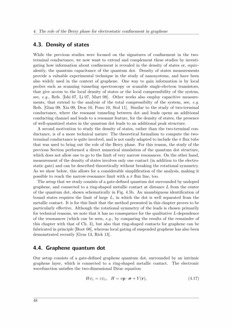
4. The role of the Berry phase for electrostatic confinement in graphene
4.3. Density of states
While the previous studies were focused on the signatures of confinement in the two-terminal conductance, we now want to extend and complement these studies by investi-gating how information about confinement is revealed in the density of states or, equiv-alently, the quantum capacitance of the quantum dot. Density of states measurementsprovide a valuable experimental technique in the study of nanosystems, and have beenalso widely used in the context of graphene. One way to gain information is by localprobes such as scanning tunneling spectroscopy or scanable single-electron transistors,that give access to the local density of states or the local compressibility of the system,see, e.g., Refs. [Ishi 07, Li 07, Mart 08]. Other works also employ capacitive measure-ments, that extend to the analysis of the total compressibilty of the system, see, e.g.Refs. [Gian 09, Xia 09, Dros 10, Pono 10, Stol 11]. Similar to the study of two-terminalconductance, where the resonant tunneling between dot and leads opens an additionalconducting channel and leads to a resonant feature, for the density of states, the presenceof well-quantized states in the quantum dot leads to an additional peak structure.
A second motivation to study the density of states, rather than the two-terminal con-ductance, is of a more technical nature: The theoretical formalism to compute the two-terminal conductance is quite involved, and is not easily adapted to include the π flux tubethat was used to bring out the role of the Berry phase. For this reason, the study of theprevious Section performed a direct numerical simulation of the quantum dot structure,which does not allow one to go to the limit of very narrow resonances. On the other hand,measurement of the density of states involves only one contact (in addition to the electro-static gate) and can be described theoretically without breaking the rotational symmetry.As we show below, this allows for a considerable simplification of the analysis, making itpossible to reach the narrow-resonance limit with a π flux line, too.
The setup that we study consists of a gate-defined quantum dot surrounded by undopedgraphene, and connected to a ring-shaped metallic contact at distance L from the centerof the quantum dot, shown schematically in Fig. 4.5b. An unambiguous identification ofbound states requires the limit of large L, in which the dot is well separated from themetallic contact. It is for this limit that the method presented in this chapter proves to beparticularly effective. Although the rotational symmetry of the leads is chosen primarilyfor technical reasons, we note that it has no consequence for the qualitative L-dependenceof the resonances (which can be seen, e.g., by comparing the results of the remainder ofthis chapter with that of Ch. 3), but also that ring-shaped contacts for graphene can befabricated in principle [Boot 08], whereas local gating of suspended graphene has also beendemonstrated recently [Grus 13, Rick 13].
4.4. Graphene quantum dot
Our setup consists of a gate-defined graphene quantum dot, surrounded by an intrinsicgraphene layer, which is connected to a ring-shaped metallic contact. The electronicwavefunction satisfies the two-dimensional Dirac equation
Hψε = εψε, H = vp · σ + V (r), (4.17)
48
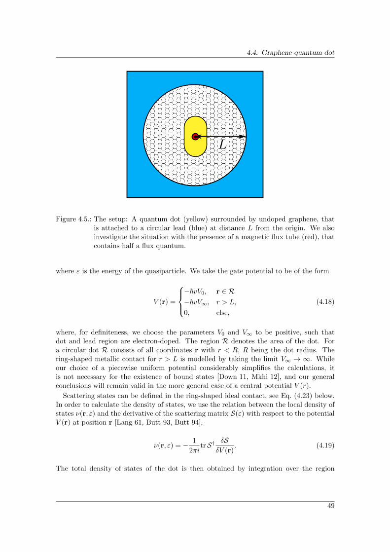
4.4. Graphene quantum dot
Figure 4.5.: The setup: A quantum dot (yellow) surrounded by undoped graphene, thatis attached to a circular lead (blue) at distance L from the origin. We alsoinvestigate the situation with the presence of a magnetic flux tube (red), thatcontains half a flux quantum.
where ε is the energy of the quasiparticle. We take the gate potential to be of the form
V (r) =
−~vV0, r ∈ R−~vV∞, r > L,
0, else,
(4.18)
where, for definiteness, we choose the parameters V0 and V∞ to be positive, such thatdot and lead region are electron-doped. The region R denotes the area of the dot. Fora circular dot R consists of all coordinates r with r < R, R being the dot radius. Thering-shaped metallic contact for r > L is modelled by taking the limit V∞ → ∞. Whileour choice of a piecewise uniform potential considerably simplifies the calculations, itis not necessary for the existence of bound states [Down 11, Mkhi 12], and our generalconclusions will remain valid in the more general case of a central potential V (r).
Scattering states can be defined in the ring-shaped ideal contact, see Eq. (4.23) below.In order to calculate the density of states, we use the relation between the local density ofstates ν(r, ε) and the derivative of the scattering matrix S(ε) with respect to the potentialV (r) at position r [Lang 61, Butt 93, Butt 94],
ν(r, ε) = − 1
2πitrS† δS
δV (r). (4.19)
The total density of states of the dot is then obtained by integration over the region
49

4. The role of the Berry phase for electrostatic confinement in graphene
r < L,1
νdot(ε) = − 1
2πi
∫r<L
drtrS† δSδV (r)
. (4.20)
The density of states νdot is defined as the density of states per spin and valley. Theexpression (4.20) is related to the Wigner-Smith time delay [Wign 55, Smit 60]. It isalso related to the dot’s capacitance [Butt 00], which can be measured from the currentresponse to an alternating bias on the ring-shaped metallic contact, at fixed value of thegate voltage V0.
The calculation of the density of states νdot at zero energy as a function of the dot po-tential V0 requires to solve the Dirac equation (4.17) at small, but finite energy ε. Dealingwith a finite energy also in the region between dot and lead goes beyond previous studiesthat adressed the two-terminal conductance, see [Bard 09, Tito 10] and the previous partof this thesis.
4.4.1. Circular quantum dot
We begin our discussion with a circular quantum dot, where the region R equals a disc ofradius R centered at the origin. In this case the angular momentum jz = (r× p)z + ~
2σzis conserved, and the solutions of the Dirac equation (4.17) can be labeled by the angularmomentum m~, where m is half-integer as a consequence of the pseudospin degree offreedom for graphene. Writing Hamiltonian (4.17) in polar coordinates (see also Sec.3.2.1),
H = −i~v(
0 ∂−∂+ 0
)+ V (r), (4.21)
with the operators
∂± = e±iθ(∂r ± i1
r∂θ), (4.22)
we solve the Dirac equation Hψε = εψε in the three regions 0 < r < R, R < r < Land r > L in which the potential V is constant. In each region, we obtain two linearlyindependent solutions,
ψ(±)k,m(r) = eimθ
√k
8v
(e−iθ/2H
(±)|m−1/2|(kr)
i sgn(m)eiθ/2H(±)|m+1/2|(kr)
), (4.23)
which describe incoming (−) or outgoing (+) circular waves of wavenumber k = (ε−V )/~vin the conduction band, normalized to unit flux. (Without loss of generality we assumethat the energy ε is positive; We checked that our final results remain valid for negative ε.)
Further, the H(±)n are Hankel functions of the first (+) and second kind (−), respectively.
The Hankel functions are related to the Bessel (Neumann) function Jn (Yn) as H(±)n =
Jn ± iYn.
1The functional derivative δS/δV (r′) can be obtained by changing the potential V (r) by v0δ(r− r′) andtaking the derivative of the scattering matrix with respect to v0. In practice, for the calculation of thedensity of states integrated over a certain region, one shifts the potential V (r) by a constant v0 withinthe specific region, and takes the derivative of the scattering matrix with respect to v0.
50

4.4. Graphene quantum dot
The precise value of the wavenumber k is different for the three regions in which thesolutions (4.23) apply. For r < R one has k ≡ k0 = ε/~v + V0; for R < r < L one hask = ε/~v, and for r > L one has k ≡ k∞ = ε/~v + V∞. For r > L the wavefunction canbe written as a linear combination of the two solutions of Eq. (4.23),
ψε,m(r) = am(ε)ψ(−)k∞,m
(r) + bm(ε)ψ(+)k∞,m
(r). (4.24)
The coefficients am(ε) and bm(ε) can be determined using continuity of the wavefunctionat r = L and r = R, as well as regularity at r = 0. They define the scattering matrixSmn(ε) = Sm(ε)δm,n through the relation
bm(ε) = Sm(ε)am(ε). (4.25)
The scattering matrix S is then used to calculate the density of states, see Eq. (4.20).To simplify the further analysis, we consider the limit of a highly doped lead k∞L 1.
In this regime, we make use the asymptotic behavior of the Hankel functions for large
arguments, H(±)n (x) ≈ (2/πx)1/2e±i(x−n
π2−π
4) for the wavefunction in the lead region r > L.
The smallness of the energy ε furthermore allows to expand in the wavenumber k in theregion R < r < L corresponding to the undoped layer separating the quantum dot fromthe lead. One then finds
Sm(ε) = e−2ik∞L+i|m|π[S(0)m + kLS(1)
m +O(ε2)], (4.26)
where k is the wavenumber in the region R < r < L,
S(0)m =
L2|m| + iJmR2|m|
L2|m| − iJmR2|m| , (4.27)
and
S(1)m =− 2i
2|m| − 1S(0)m +
8i|m|L4|m| + 2i[(2|m|+ 1)J 2m − (2|m| − 1)]R2|m|+1L2|m|−1
(4|m|2 − 1)(L2|m| − iJmR2|m|)2
(4.28)
if |m| 6= 1/2, whereas
S(1)±1/2 =
i(L2 −R2) + 2iJ 212
R2 log(L/R)
(L− iJ 12R)2
. (4.29)
In Eqs. (4.27)–(4.29) we used the abbreviation
Jm =J|m|+1/2(k0R)
J|m|−1/2(k0R). (4.30)
We now use Eq. (4.20) to calculate the density of states νdot at zero energy,
νdot =1
2πi~v∑m
S(0)∗m
[∂S(0)
m
∂V0+ LS(1)
m
]. (4.31)
51

4. The role of the Berry phase for electrostatic confinement in graphene
The first term in Eq. (4.31) represents the integral of the local density of states inside thequantum dot region r < R; the second term is the integral of the local density of states inthe undoped layer that separates the dot and the metallic contact.
Let us now analyse the density of states as a function of the gate voltage V0. In the limitR L (weak coupling to the ring-shaped contact), the DOS exhibits isolated resonancesat gate voltages V0 = V ′0 satisfying the condition
J|m|−1/2(V ′0R) = 0. (4.32)
Close to resonance, we have that Jm ≈ −1/[R(V0 − V ′0)], and the density of states hasa Lorentzian dependence on V0. For a generic resonance with |m| 6= 1/2 the zero-energydensity of states has the form
νdot =4R|m|
π~v(2|m| − 1)
Γ
4R2(V0 − V ′0)2 + Γ2, (4.33)
where the dimensionless resonance width is given by
Γ = 2(R/L)2|m|. (4.34)
Resonances are well separated if R L. In the lowest angular momentum channel|m| = 1/2 the expression for the density of states reads
νdot =2R
π~v
(1 + log
L
R
)Γ
4R2(V0 − V ′0)2 + Γ2, (4.35)
with Γ = 2R/L. We remark that the position of the resonances, as well as the scaling ofthe width agree with the results for the two-terminal conductance, where L is the distancebetween source and drain.
We note, that the resonant part of νdot that comes from the first term in Eq. (4.31) inte-grates to 1/~v, when integrated over V0, corresponding to a 2π shift of the scattering phaseupon tuning V0 through a resonance. The second term in Eq. (4.31) gives an additionalcontribution to the density of states, whose weight decays for higher angular momentum.Remarkably, in the lowest angular momentum channel, this additional contribution has alarge factor log(L/R) factor in the prefactor. We relate the presence of this large factor tothe fact, that the bound states of the lowest angular momentum have only a slow decay∝ 1/r, such that the wavefunction is marginally non-normalizable, see Sec. 3.2.1.
We show a plot of the density of states for a circular quantum dot as a function ofthe gate voltage in Fig. 4.6. As discussed, the DOS exhibits resonant peaks, that can belabelled according to their angular momentum channel, and the position is given by Eq.4.32. The higher the angular momentum, the sharper the resonances, consistent with thescaling of the width Eq. (4.34).
4.4.2. Chaotic quantum dot
We now extend our analysis to a quantum dot of arbitrary geometry. For the genericsituation, the scattering matrix is no longer diagonal in the angular momentum basis and
52

4.4. Graphene quantum dot
Figure 4.6.: Density of states for a circular quantum dot. Resonances are labelled accord-ing to their angular momentum |m| (R/L = 0.2).
an analytical solution is no longer available. We pursue a numerical approach for thecalculation of the scattering matrix instead.
Our numerical method follows the calculation of the scattering matrix in Ch. 3. Theproblem is broken up into thin circular slices, for which the scattering effect is weak andmay be captured in Born approximation. The scattering matrix of the full system is thenobtained by subsequent concatenation of the scattering matrices of the slices. A differencewith Ch. 3 is that we have to calculate the scattering matrix at a finite energy or potentialin order to evaluate Eq. (4.20). Since the quantum dot has a finite size, the numericalevaluation is necessary up to a distance R away from the origin only. (For the geometryshown in Fig. 4.7, one has R = R + a). For R < r < L the analytical calculationsoutlined above can be used. We refer to Appendix B.2 for further details of the numericalimplementation.
As a prototypical example of a chaotic dot, we now investigate the density of states fora stadium-shaped quantum dot. In Fig. 4.7, we show the result of a calculation of thedensity of states as a function of the gate voltage V0. We find a series of resonances ofsimilar width. The width is comparable to that of the broadest resonances for the circulardot, in agreement with the general expectation that confinement is suppressed in chaoticdots.
To further analyze the situation, we zoom in on the first resonance and investigate itsdependence on the strength of the dot-lead coupling R/L, see Fig. 4.8. We extract heightand width of the resonance by fitting to a Lorentzian,
νdot =2RA~πv
Γ
4R2(V0 − V ′0)2 + Γ2, (4.36)
where V ′0 is the resonance position. For the chaotic structure, we expect the resonant statesto be composed as a mixture of all angular momentum channels. In the limit of large L/Rwe expect that the lowest possible angular momentum channel |m| = 1
2 is dominant. The
53

4. The role of the Berry phase for electrostatic confinement in graphene
Figure 4.7.: Density of states for a stadium quantum dot. (R/L = 0.2, 2a/R =√
3.)
behavior of the resonances should then resemble those of a |m| = 12–resonance of a circular
dot, i.e., we expect width and amplitude to scale as
Γ = aR
L, (4.37)
A = b+ c logL
R, (4.38)
with coefficients a, b, and c of order unity. The numerical study indeed verifies thisassertion, as can be seen from the inset of Fig. 4.8. We further checked, that the otherresonances of Fig. 4.7 show the same behavior for sufficiently small values of R/L, althoughthe onset of the asymptotic small-R/L behavior and the precise values of the numericalcoefficients a, b, and c vary from resonance to resonance. We attribute these variations tothe different constitutions of the resonances, indicating the relative weigth of the |m| = 1
2channel for a certain resonance in comparison to higher angular-momentum channels. Wefurther verified, that the position of the resonances agrees with the ones obtained in acalculation of the conductance (Ch. 3).
To summarize: For a regular quantum dot, we find signatures of well-confined states,that become very sharp in the limit of weak coupling between dot and lead, as well asbroad resonances with a width scaling ∝ R/L upon changing the coupling to the lead.For the chaotic dot, we observe such “broad” resonances only. The results for the densityof states are consistent with the results for a two-terminal conductance setup.
4.5. Effect of a π-flux
The difference between regular and chaotic quantum dots in graphene becomes much morepronounced, when we introduce a magnetic flux carrying half a flux quantum. Electronsencircling this flux tube acquire an Aharonov-Bohm phase of π, which cancels the Berryphase that the electronic wavefunction collects via the pseudospin upon performing a
54

4.5. Effect of a π-flux
Figure 4.8.: Density of states for the first resonance, as well as resonance height A andwidth Γ (insets) of the stadium dot for various values of the ratio R/L.(2a/R =
√3.)
circular motion. The magnetic flux shifts the kinematic angular momentum to integervalues, allowing for a state that cannot be confined by gate potentials.
We now analyse the density of states for a graphene quantum dot in the presence ofsuch π-flux. For this, we add the vector potential
A(r) =~e
1
2reθ. (4.39)
Inclusion of A(r) into the Dirac equation amounts to making the replacement ∂± → D±in Eq. (4.21), with (see also Sec. 4.1)
D± = e±iθ(∂r ± i1
r∂θ ∓12r
). (4.40)
We further introduce the kinematic angular momentum,
jz,kin = [r× (p + eA)]z + ~2σz (4.41)
For the π-flux (4.39), the kinematic angular momentum is related to the canonical angularmomentum as jz,kin = jz + ~/2, and therefore is quantized in integer multiples of ~. Wenow consider the effect of a π-flux line on the density of states in a circular and chaoticquantum dot separately.
4.5.1. Circular dot
For the circular dot the flux line is positioned in the origin, so that rotational symmetry ispreserved. The calculation for the density of states proceeds in an analogous way as in thecase without flux line. The presence of the flux modifies the basis wavefunctions (4.23).We label the new basis states by the integer index of the kinematic angular momentum µ,
jz,kinψ(±)k,µ = µ~ψ(±)
k,µ . (4.42)
55
4. The role of the Berry phase for electrostatic confinement in graphene
For non-zero µ, the basis states now read
ψ(±)k,µ (r) =
√k
8v
(ei(µ−1)θH
(±)|µ−1/2|(kr)
i sgn(µ)eiµθH(±)|µ+1/2|(kr)
), (4.43)
while for zero kinematic angular momentum, we find
ψ(±)k,0 (r) =
e±ikr√4πrv
(±e−iθ
1
). (4.44)
The state with zero kinematic angular momentum needs to be discussed separately, andwill be responsible for the crucial difference caused by the magnetic flux. Let us discussthe states with non-zero kinematic angular momentum first, where the magnetic flux onlyleads to slight modifications. Indeed, one finds that the results of Eqs. (4.27)-(4.28) remainvalid, provided the half-integer index m is replaced by the integer index µ, which labelskinematic angular momentum. In particular, resonances in the density of states nowappear at roots of half-integer Bessel function J|µ|−1/2(V0R) = 0, and the resonance width
is Γ = 2(R/L)2|µ|.For the case µ = 0 regularity of the wavefunction at the origin is not sufficient to deter-
mine the scattering matrix S0(ε). This problem can be cured by a suitable regularizationof the flux line. Taking a flux line of extended diameter we find the condition that theupper component of the wavefunction has to vanish at the origin (see Sec. 4.1). With thisregularization the calculation of the scattering matrix S0(ε) is straightforward and has theresult
S0 = e−2i(k∞−k0)Re−2i(k∞−k)(L−R), (4.45)
where k = ε/~v and k0 = ε/~v+V0. This scattering matrix gives a constant, non-resonantcontribution to the density of states, which will be disregarded in the considerations thatfollow because it is independent of the gate voltage V0.
We show the density of states for a circular quantum dot in the presence of a fluxtube in Fig. 4.9. It contains resonances originating from non-zero angular momentumchannels. The position and the width of such resonances has been discussed above. Thezero-angular momentum channel has no V0-dependent contribution to the density of states.Our findings are consistent with a simulation of the two-terminal transport, concerningthe position and the scaling of the width upon changing R/L of the resonances (Sec. 4.2)although the regime of small R/L could not be accessed there.
4.5.2. Chaotic Dot
The numerical method described in Sec. 4.4.2 and the appendix can be easily carried overto the case with the π-flux, by taking the wave functions Eqs. (4.43) and (4.44) instead ofEq. (4.23). One has to pay attention to the boundary condition at the origin for the zeroangular momentum channel, as discussed above.
We show the result of a calculation of the density of states of a stadium-shaped quantumdot in the presence of a flux tube in Fig. 4.10, as a function of the dot’s potential. The
56

4.5. Effect of a π-flux
Figure 4.9.: Density of states for a circular quantum dot in the presence of a flux tube.Resonances are labelled according to their kinematic angular momentum |µ|.(R/L = 0.2.)
flux tube is placed off-center in order to lift a twofold rotation symmetry. We observe adensity of states with broad peaks, the peak widths typically being much larger than for thecircular dot (compare with Fig. 4.9). The analysis can be made quantitative by consideringa specific “peak” as a function of R/L, see Fig. 4.11. Remarkably, the density of statessaturates in the limit R/L→ 0 that corresponds to a weak coupling between the quantumdot and the ring-shaped metallic contact. This behavior is a qualitative difference withthe case of a circular dot and clearly distinguishes resonances of a chaotic dot with fluxfrom those of a regular dot or the situation without flux. We explain this feature by thespecial role of the zero angular momentum channel, that becomes dominant decay channelin the limit of small R/L. As this channel is not capable of binding (or backscattering)states, the density of states becomes insensitive of the distance L to the metallic contact.The transient behavior for R/L of order unity is attributed to the contribution from finite-angular-momentum channels to the resonance width, which gradually disappears if R/Lbecomes small.
For the specific resonance shown in Fig. 4.11, the saturation of the density of statestakes place only for very small dot sizes. On the other hand, the absence of a boundstate may also be inferred from an analysis of the width of the resonance-like feature asa function of R/L. Obtaining the width Γ from a Lorentzian fit, the inset of Fig. 4.11shows that Γ approaches a finite value as R/L goes to zero, with a leading correction∝ (R/L)2, which we attribute to a contribution from the angular momentum channel|µ| = 1. Such behaviour is in stark contrast to the scenario without flux tube, where thewidth goes to zero in the limit R/L → 0. We verified the same qualitative behavior forthe other resonance-like features shown in Fig. 4.10, where the value of R/L, at which thewidth saturates, varies considerably for different resonances, expressing the variations ofthe relative contribution in the channel of zero angular momentum. We also found roughagreement in the positions of the resonances with the ones obtained in the calculation
57

4. The role of the Berry phase for electrostatic confinement in graphene
Figure 4.10.: Density of states for a stadium-shaped quantum dot in the presence of aπ-flux tube. The flux is shifted from the center of the stadium in order tobreak inversion symmetry und obtain a truly chaotic structure, see also Sec.4.2. (R/L = 0.2, 2a/R =
√3, d = 2a/3.)
of the conductance (Sec. 4.2), although no precise comparison is possible here, since theresonances cannot be made arbitrarily narrow upon making the dot smaller. We note,that our calculation of the density of states allows us to access for much smaller valuesof R/L as compared to the numerical study of the two-terminal conductance in Sec. 4.2,including access to the regime, where the lineshape of the density of states saturates.
4.6. Conclusion
In this Chapter we investigated the observation of Chapter 3, that the two-terminal con-ductance of a generic gate-defined graphene quantum dot shows resonances in the limit ofa weak coupling to the leads, in spite of the naive expectation that electrons can not beconfined in such a quantum dot because of Klein tunneling. We attribute this observationto the Berry phase in graphene, which quantizes angular momenta to half-integer values.With half-integer angular momenta, strict perpendicular incidence — the condition forKlein tunneling with unit probability — does not occur. As a consequence, conductanceresonances exist in both integrable and chaotic geometries. The only difference betweenthe two cases is a quantitative one: it concerns the scaling of the resonance widths withthe coupling to the leads.
The Berry phase can be cancelled against an Aharonov-Bohm phase, when a flux tubecontaining half a flux quantum is introduced to the system. With a magnetic flux tube,we showed that the relevant angular momentum, the kinematical angular momentum, isquantized to integer values. In this case a state with zero angular momentum is possible.Such a state can not form a bound state or give rise to a conductance resonance. Weshowed this by an explicit calculation for the disc-shaped quantum dot in Sec. 4.1, andusing numerical calculations for disc-shaped and stadium-shaped quantum dots in Sec.
58

4.6. Conclusion
Figure 4.11.: Density of states for the first “resonance” and the corresponding resonancewidth (inset) of the stadium dot for various values of the ratio R/L. Bothheight and width of the feature saturate in the limit R/L → 0. (2a/R =√
3, d = 2a/3.)
4.2. Once the Aharonov-Bohm phase from the π-flux tube cancels the Berry phase, theresults of the full quantum theory are consistent with the simple classical expectations.With a π-flux, there is a stark qualitative difference between conductance resonance forintegrable and non-integrable quantum dots: Whereas sharp conductance resonances forthe case of an integrable quantum dot continue to exist, in the limit of weak lead-dotcoupling the conductance becomes featureless for a generic non-integrable quantum dot.
We further explored the density of states as an alternative signature of confinement inthis chapter. As we have shown, the calculation of the density of states is significantlyeasier than the calculation of the two terminal conductance, which allows us to extendthe analysis to quantum dots with a flux line (in order to highlight the role of the Berryphase associated with the graphene pseudospin) and to access the regime of well isolatedresonances, which requires the limit that the metallic contacts are far away from thequantum dot. This limit could not be reached in numerical simulations of the two-terminaltransport.
The strong influence of the geometry on the capability of the quantum dot to confinestates can also be deduced from our calculation of the density of states. While bothregular and chaotic dot have resonant signatures in the density of states, the scalingof the width of these features with the (linear) size L of the undoped graphene layerseparating the dot and the metallic contacts allows to discern the geometries: While forthe chaotic dot, all resonances have a width scaling proprotional to 1/L, indicating a weakconfinement, for the regular dot, most of the resonances have a width that vanishes fasterupon increasing L, indicating well-confined states. The difference between chaotic andintegrable geometries becomes much more pronounced, when a flux tube carrying half aflux quantum is introduced to the system. In this case, in the limit of large L the lineshapefor the density of states for the chaotic dot saturates — corresponding to a “resonance
59

4. The role of the Berry phase for electrostatic confinement in graphene
width” that is independent of L. Such behavior signals the absence of confined states, incontrast to the case of a disc-shaped dot, that continues to show sharp resonances after aflux tube has been inserted.
The analysis carried out in this chapter considered the density of states integratedover the dot and the surrounding undoped graphene sheet. On the other hand, scanningtunneling microscope experiments measure a local density of states for the region coveredby the tunneling tip. The formalism that we developed here can easily be extended tothis kind of measurement setup. As far as a qualitative analysis of peak widths and peakpositions goes, however, we expect no difference between the local density of states andthe integrated density of states that was studied here.
60
5. Semiclassical theory of the interactioncorrection to the conductance of antidotarrays
The wave nature of electrons manifests itself in a number of signatures in the electric trans-port of disordered metals, such as weak localization, universal conductance fluctuations, orinteraction-induced effects like the Altshuler-Aronov correction to the conductivity. Thequalitative effect of these features is successfully explained on a semiclassical level, basedon classical electronic trajectories through the solid, while the quantitative analysis is typ-ically reserved to powerful field-theoretical methods, such as diagrammatic perturbationtheory. In recent years however, semiclassical methods have been enormously improved,such that also a quantitative description of these quantum effects in transport is possi-ble nowadays. The semiclassical description differs from a field-theoretical description bythe appearence of an additional timescale — the so-called Ehrenfest time, which sets aminimal time below which wave effects are not operative.
Noninteracting effects as weak localization and universal conductance fluctuations havebeen intensively studied by semiclassical methods in past years. This chapter aims ata semiclassical description for the interaction correction to the electrical conductivity.Subsequent to an introduction, we develop the semiclassical theory for the interactioncorrection of a generic conductor in Sec. 5.2. We then illustrate the effects in quasi-oneand two-dimensional antidot arrays, which represent experimentally relevant examples ofsystems that require a semiclassical approach (Sec. 5.3). We conclude our results in Sec.5.4.
The content of this chapter is based on the publication [Schn 13].
5.1. Introduction
Electronic transport in weakly disordered metals is successfully described by the Boltz-mann theory, in which electrons are treated as effectively classical particles moving freelybetween scattering events. The wave nature of electrons gives rise to a number of correc-tions to transport properties, such as the weak localization correction [Ande 79, Gork 79],the Altshuler-Aronov interaction correction [Alts 79, Alts 85b], or the universal conduc-tance fluctuations [Alts 85a, Lee 85]. Weak localization results from the constructive in-terference of electrons propagating along time-reversed paths [Chak 86]. The physicalintuition behind the interaction correction is constructive interference of electron trajec-tories which are scattered on impurities and Friedel oscillations of the electron density[Rudi 97, Zala 01]. These quantum corrections become increasingly important as thetemperature is lowered, the effective dimensionality of the sample is reduced, or as the
61
5. Semiclassical theory of the interaction correction to the conductance of antidot arrays
disorder level is increased. They have a distinctive and universal dependence on externalparameters, such as temperature or magnetic field, which makes them identifiable in exper-iments. In particular, the two quantum corrections to the conductivity, weak localizationand the Altshuler-Aronov correction, can be distinguished by application of a magneticfield, since weak localization is suppressed by already a very small magnetic field, whereasthe Altshuler-Aronov correction is not.
A “classical analog” of a disordered metal is realized in high-mobility semiconductorstructures with randomly placed large antidots [Rouk 89, Enss 90]. The absence of im-purities ensures that electrons move ballistically between reflections off the antidots. Thereason why these systems are referred to as classical is that the size of the antidots a ismuch larger than the Fermi wavelength λF. As a result, not only the electron’s motionthrough the two-dimensional electron gas, but also the reflection off an antidot is de-scribed by classical mechanics. (In contrast, in a disordered metal, the size of impuritiesis comparable to λF, so that the scattering event is strongly diffractive.) For an irregulararrangement of antidots, the classical dynamics is chaotic. Nearby trajectories separateexponentially in time, the exponential separation being characterized by the Lyapunovcoefficient λ. The chaotic dynamics is essential for the existence of quantum correctionsin this system, as it magnifies the quantum uncertainty of even a minimal wavepacket upto classical dimensions within the short time
τE =1
λln(a/λF), (5.1)
thus transforming the classical dynamics into quantum-diffractive dynamics on time scaleslarger than τE [Alei 96]. The time τE is known as the “Ehrenfest time”.
Since wave effects are not operative for times shorter than τE — electrons essentiallymove along classical trajectories up to the Ehrenfest time —, the Ehrenfest time servesas a short-time threshold for the duration of the trajectories contributing to the quantumcorrections in an antidot array. For weak localization, it was found that the correctionto the conductivity is exponentially suppressed if τE is larger than the dwell time τD, thetypical time to be transmitted through the system, or the dephasing time τφ [Alei 96,Adag 03, Brou 07, Tian 07]. In contrast, other quantum corrections, such as the universalconductance fluctuations, remain finite if τE τD [Twor 04, Jacq 04, Brou 06, Brou 07].
The goal of this chapter is to present a theory of the Ehrenfest-time-dependence ofthe Altshuler-Aronov correction δGAA. The analysis presented here significantly extendsa previous calculation by Kupferschmidt and Brouwer [Brou 08], which studied the τE
dependence of the interaction correction to the conductance of a ballistic double quantumdot and found that δGAA is strongly suppressed if τE exceeds the dwell time τD or theinverse temperature ~/T . The double quantum dot studied in Ref. [Brou 08] is the simplestsystem with nonzero Altshuler-Aronov correction to the conductance, and is characterizedby a long-range interaction, which is spatially homogeneous within each dot. The theorypresented here is valid for both short-range and long-range interactions and can be appliedto any geometry in which the classical electron dynamics is chaotic — although we willfocus our discussion on the case of an antidot array. For the general case consideredhere we confirm the suppression of δGAA for τE min(τD, ~/T ) and we calculate theprecise functional dependence of δGAA on τD and T for finite Ehrenfest time. The explicit
62

5.2. Semiclassical theory of the interaction correction
dependence on temperature is characteristic for the interaction correction, which has itsorigin in virtual processes with an energy transfer larger than temperature.
Our calculation makes use of a semiclassical formalism that starts from the saddle-pointapproximation around classical trajectories for the single-particle Green function. In thisway, the conductance in the absence of electron-electron interactions is written as a doublesum over classical trajectories that connect source and drain reservoirs [Jala 90, Bara 93].Weak localization and other quantum corrections to the conductance then follow fromspecial configurations of trajectories, in which the two trajectories in the summation arepiecewise paired, and proceed through “crossings” at points where the pairing is changed[Rich 02, Mull 07]. In the language of diagrammatic perturbation theory, segments wherethe trajectories are paired correspond to diffusons or cooperons, whereas the crossings cor-respond to Hikami boxes. The application to interacting electrons requires a modificationof the formalism, which will be described in detail below.
Our analysis applies to a “ballistic” conductor, where the label “ballistic” is meant tospecify that the electrons move along well-defined classical trajectories. In the literature,“ballistic” sometimes refers to a different limit, and several calculations of the interactioncorrection to the conductance have been reported for such “ballistic limits”. Whereasthe original work of Altshuler and Aronov [Alts 79] addressed a disordered metal withshort-range scatterers in the diffusive regime Tτ 1, the theory was generalized to ac-count for the effects of higher temperatures Tτ & 1, a regime referred to as “ballistic”[Gold 86, Das 99, Zala 01]. The case of a smooth disorder potential, in which scatter-ing is predominantly forward, was considered in Ref. [Gorn 04]. Another type of system,where interaction corrections appear, are networks of capacitively coupled ballistic quan-tum dots [Belo 03, Golu 04, Kupf 08], where, however, Ehrenfest-time-related phenomenacan be neglected as long as τE is much smaller than the dwell time in a single quantumdot. Interactions also affect the conductance through their effect on the weak localizationcorrection (dephasing). Semiclassical studies of the effect of interaction-induced dephas-ing on weak localization can be found in Refs. [Yevt 00, Tian 07, Peti 07, Whit 08], forelectronic systems and in Ref. [Hart 12] for bosonic matter waves.
5.2. Semiclassical theory of the interaction correction
In this section we present the semiclassical description of the interaction corrections fora conductor with a well-defined chaotic classical electron dynamics. We first review theexpressions for the interaction corrections to the conductance in terms of the single-particleGreen function, and then apply the semiclassical approximation methods, taking intoaccount the finite Ehrenfest time.
5.2.1. Skeleton diagrams for the conductance
For definiteness, we consider a two-dimensional ballistic conductor, such as a ballisticelectron gas with an antidot array, in contact with reservoirs at x = 0 and x = L, see Fig.5.1. Without interactions, we can calculate the conductance G from the Kubo formula
63

5. Semiclassical theory of the interaction correction to the conductance of antidot arrays
Figure 5.1.: Schematic picture of the system under consideration: A ballistic conductor,attached to ideal leads at x = 0 and x = L. In the semiclassical calculation ofthe conductance, one retarded and one advanced Green function are attachedto a current vertex located at the interface with the leads. In a semiclassicalpicture, these Green functions are associated with “retarded” and “advanced”classical trajectories (solid and dashed in the figure), both of which must pointinto the conductor (1). A current vertex combined with two Green functionsof the same kind is not possible for the calculation of the conductance: af-ter pairing, we have trajectories that go straight into the leads (2). On thecontrary, for a calculation of the conductivity, the current vertex can be any-where inside the conductor, and pairing of retarded and advanced trajectoriesis possible also if two Green functions of the same kind are attached to onecurrent vertex (3 and 4).
[Akke 07],
G =e2~π
∫dy
∫dy′∫dξ
(−∂f(ξ)
∂ξ
)[vxGR(r, r′; ξ)vx′GA(r′, r; ξ)
]x′=0x=L
, (5.2)
where f(ξ) = 1/(exp(ξ/T ) + 1) denotes the Fermi function,
vx =~
2mi
(−→∂x −
←−∂x
)(5.3)
is the velocity operator, and GR(r, r′; ξ) and GA(r, r′; ξ) is the retarded and advancedsingle-particle Green function, respectively. Retarded and advanced Green functions arerelated as
GA(r′, r; ξ) = GR(r, r′; ξ)∗. (5.4)
To leading (first) order in the interaction strength, the interaction correction δGAA isobtained by replacing GR(r, r′; ξ) by GR(r, r′; ξ)+δGR
F (r, r′; ξ)+δGRH(r, r′; ξ) and expanding
64
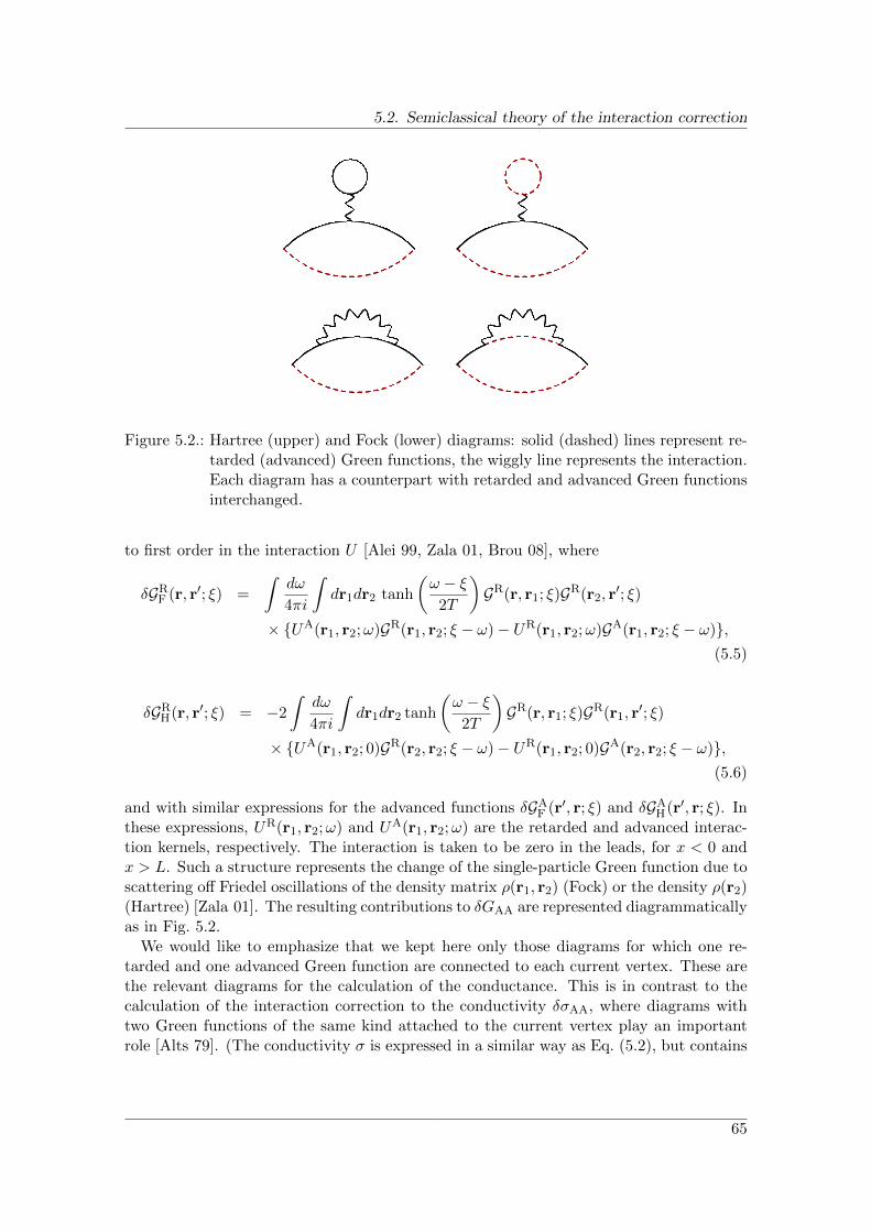
5.2. Semiclassical theory of the interaction correction
Figure 5.2.: Hartree (upper) and Fock (lower) diagrams: solid (dashed) lines represent re-tarded (advanced) Green functions, the wiggly line represents the interaction.Each diagram has a counterpart with retarded and advanced Green functionsinterchanged.
to first order in the interaction U [Alei 99, Zala 01, Brou 08], where
δGRF (r, r′; ξ) =
∫dω
4πi
∫dr1dr2 tanh
(ω − ξ
2T
)GR(r, r1; ξ)GR(r2, r
′; ξ)
× UA(r1, r2;ω)GR(r1, r2; ξ − ω)− UR(r1, r2;ω)GA(r1, r2; ξ − ω),(5.5)
δGRH(r, r′; ξ) = −2
∫dω
4πi
∫dr1dr2 tanh
(ω − ξ
2T
)GR(r, r1; ξ)GR(r1, r
′; ξ)
× UA(r1, r2; 0)GR(r2, r2; ξ − ω)− UR(r1, r2; 0)GA(r2, r2; ξ − ω),(5.6)
and with similar expressions for the advanced functions δGAF (r′, r; ξ) and δGA
H(r′, r; ξ). Inthese expressions, UR(r1, r2;ω) and UA(r1, r2;ω) are the retarded and advanced interac-tion kernels, respectively. The interaction is taken to be zero in the leads, for x < 0 andx > L. Such a structure represents the change of the single-particle Green function due toscattering off Friedel oscillations of the density matrix ρ(r1, r2) (Fock) or the density ρ(r2)(Hartree) [Zala 01]. The resulting contributions to δGAA are represented diagrammaticallyas in Fig. 5.2.
We would like to emphasize that we kept here only those diagrams for which one re-tarded and one advanced Green function are connected to each current vertex. These arethe relevant diagrams for the calculation of the conductance. This is in contrast to thecalculation of the interaction correction to the conductivity δσAA, where diagrams withtwo Green functions of the same kind attached to the current vertex play an importantrole [Alts 79]. (The conductivity σ is expressed in a similar way as Eq. (5.2), but contains
65
5. Semiclassical theory of the interaction correction to the conductance of antidot arrays
integrals over the x-coordinates as well, rather than fixing them to the contacts at x = 0and x = L). Although the structure of the calculation for conductance or conductivityconsiderably differs, the final results for these quantities are related by a geometrical factoronly. In two dimensions, for a rectangular sample, one has G = σWL , where W is the widthof the system.
The difference between the conductance calculation and the conductivity calculation isreadily seen in the semiclassical language. In that language, Green functions are associatedwith classical trajectories, and only terms in which “retarded” and “advanced” trajectoriesare paired contribute. (For more details, see below). Since the leads are assumed to befree of disorder and without electron-electron interactions, both the retarded and theadvanced trajectories at the positions r and r′ in Eq. (5.2) must point into the conductorif the conductance is calculated. On the other hand, for a current vertex in the system’sinterior, pairing of advanced and retarded trajectories is still possible even if two Greenfunctions of the same kind are attached to the current vertex, see Fig. 5.1.
The fact that different diagrams are needed for the calculation of conductance andconductivity is well known, the same is true for the Drude conductance and conductancefluctuations of a disordered metal (see Ref. [Kane 88]). For instance, for the calculationof the Drude conductivity σ0 in a metal with short-ranged disorder there is no need todress the diagram with an impurity ladder, while for the classical conductance G0, thediagram dressed with an impurity ladder, i.e., a diffuson, is most relevant. For the Drudeconductivity one might argue that the distance between the current vertices is of the orderof the mean free path, since the two Green functions decay on this scale. The diffuson inturn is long-ranged, and hence needed to describe propagation from one lead to the other,as required for the conductance.
We also note that the calculation of the conductance as it is outlined here is similar tothe calculation of the density-density correlation functions [Fink 83, Cast 84]. A subtlepoint in this regard is the existence of additional corrections in the calculation of thedensity-density correlation function, namely vertex corrections and the so-called wave-function renormalization. In the description developed below, both of them appear tovanish. For the density-density correlation function, in turn, vertex corrections and thewave function renormalization cancel each other, so that these corrections do not lead toa net change of the result in either case.
5.2.2. Semiclassical theory
The conductance G depends on the precise locations of antidots, the system boundary,and on the Fermi energy. We now employ a semiclassical analysis in order to identify thosecontributions to the conductance that remain after an average over the Fermi energy.
Starting point is the semiclassical expression of the Green function GR(r, r′; ξ) as a sumover classical trajectories α from r′ to r at energy ξ [Gutz 90],
GR(r, r′; ξ) =2π
(2πi~)3/2
∑α
AαeiSα/~. (5.7)
Here, Sα(r, r′; ξ) is the classical action corresponding to the trajectory α, which has the
66

5.2. Semiclassical theory of the interaction correction
properties∂Sα∂r
= pα,∂Sα∂r′
= −p′α, (5.8)
and∂Sα∂ξ
= τα, (5.9)
where pα and p′α denotes the momentum at the end and beginning of α, respectively,and τα is the duration of the trajectory. The stability amplitude Aα is given by Aα =√|det(Dα)|, with
Dα =
(∂2Sα∂r′∂r
∂2Sα∂r′∂ξ
∂2Sα∂ξ∂r
∂2Sα∂ξ2
). (5.10)
The semiclassical Green function further contains an additional phase-shift, the so-calledMaslov index [Gutz 90], which we omitted because it does not play a role in our con-siderations. The semiclassical expression for advanced Green function follows from Eq.(5.4).
Using the semiclassical Green function (5.7) we express the interaction correction δGAA
as a fourfold sum over classical trajectories. We refer to these trajectories as “retarded” or“advanced”, depending on the type of the Green function that they originate from. Thesummation over classical trajectories can be simplified for a system with chaotic classicaldynamics: In this case, the classical trajectory and hence the classical action depend verysensitively on the initial conditions. On the other hand, in the semiclassical limit ~ → 0only configurations of trajectories with sum of the actions of the “retarded” trajectoriessystematically equal to the sum of the actions of the “advanced” trajectories up to adifference ∆S of the order of ~ contribute substantially to the conductance. This occursonly if the “retarded” and “advanced” trajectories are piecewise paired, whereby they canexchange “partners” only at a “small-angle encounter” [Rich 02], at which two pairs meetto within a phase-space distance of order ~1/2.
For the remaining summation over trajectories, we use a sum rule that expresses thesummation over trajectories α between positions r′ and r and at energy ξ in terms of anintegral over the trajectory’s duration t, the initial and final momenta p′ and p, as wellas a “trajectory density” ρξ(X
′ → X; t) between the phase-space points X′ = (r′,p′) andX = (r,p) [Arga 95, Arga 96],∑
α:r′→r;ξ
A2αf(p′α,pα, τα) =
∫ ∞0
dt
∫dp′ξ
∫dpξρξ(X
′ → X; t)f(p′,p, t), (5.11)
see App. C.1.1 for details. Here f is an arbitrary function. The initial point in phase spaceX′ = (r′,p′), together with the Hamilton function H uniquely determines the classicaltrajectory, and after a time t this trajectory has reached the phase space point X(t) =(r(r′,p′; t),p(r′,p′, t)). The trajectory density
ρ(X′ → X; t) = δ[X−X(t)] (5.12)
= δ[r− r(r′,p′; t)]δ[p− p(r′,p′; t)]
selects then only those phase space points which are connected by a trajectory of durationt. At fixed energy ξ, the momentum integrations are restricted to the energy shell, dpξ =
67

5. Semiclassical theory of the interaction correction to the conductance of antidot arrays
Figure 5.3.: Configuration of trajectories relevant for the first diagram to the Fockcontribution.
dpδ(ξ−H(p, r)), and for the trajectory density we may factor out the part which ensuresenergy conservation,
ρ(X′ → X; t) = ρξ(X′ → X; t)δ[H(X)−H(X′)]. (5.13)
The factor A2α provides the Jacobian for this transformation.
Following the procedure outlined so far, we obtain an expression in terms of trajectorydensities which, strictly speaking, is a sum of δ-functions. We then replace the exacttrajectory density ρξ by a coarse-grained smooth density ρ [Smil 92, Arga 93]. The coarsegraining takes place with respect to small fluctuations of the initial and final phase spacepoints and/or the positions of the scattering discs or the system’s boundaries. In theregime λτD 1, where the chaotic dynamics has fully developed, the classical dynamicsis essentially stochastic, which justifies the coarse graining procedure. The coarse-grainedtrajectory density
ρξ(X′ → X; t) = P (X,X′; t) (5.14)
can be identified with the probability density P (X,X′; t) that a particle originating at thephase space point X′ = (r′,p) is found at the phase space point X = (r,p) after a timet. (Since we are interested in the regime where temperature is much smaller than Fermienergy, we drop the dependence of the classical propagators on ξ.) For the case of antidotarrays, this probability density is described by a diffusion equation.
The Drude conductance is obtained by keeping only pairs of classical trajectories thatconnect source and drain reservoirs. Following the steps described above, we find
G0 =e2
2π2~2
∫ ∞0
dt
∫dydy′
∫dpξdp
′ξ
[vxP (X,X′; t)v′x
]x′=0x=L
(5.15)
We now turn to the semiclassical calculation for the interaction correction.
5.2.3. Fock contribution
We start with the Fock contribution to δGAA, which is given by the two lower diagramsin Fig. 5.2, together with their counterparts, which are obtained by interchanging theretarded and advanced Green functions. We first consider the conductance correction
68

5.2. Semiclassical theory of the interaction correction
δGF,1AA from the lower left diagram and its counterpart, which reads
δGF,1AA = −e
2~π
∫dξ
(−∂f(ξ)
∂ξ
)∫dω
2πtanh
(ω − ξ
2T
)Im
∫dr1dr2U
R(r1, r2;ω)
×∫dy
∫dy′[vxGR(r, r′; ξ)vx′GA(r′, r2; ξ)GA(r2, r1; ξ − ω)GA(r1, r; ξ)
]x′=0x=L
.
(5.16)
After insertion of the semiclassical expression Eq. (5.7) for the Green functions, we obtaina sum over one retarded and three advanced trajectories. In the semiclassical limit, aconvolution of Green functions is customarily calculated using the stationary phase ap-proximation. For this one first needs to determine the configurations of trajectories whichmake the total action stationary. This results in a factor ∝ eiSst , where Sst is obtained byinserting the stationary configuration into the total action. Integration over quadratic fluc-tuations around the stationary configurations then renders the prefactor. In the presentcase the convolution of Green functions is accompanied by the interaction propagator. Onemight expect, that the interaction propagator affects the stationary trajectories, such thatthey no longer connect to a single classical trajectory, as in the case without interaction.However for the calculation of the conductance, we need to pair the advanced trajectorieswith the retarded one, see Fig. 5.3. Hence, performing the integration over r1 and r2 inEq. (5.16) within stationary phase approximation, we only take into account stationaryconfigurations that connect to a single classical trajectory. The detailed calculation iscarried out in Appendix C.1.2 and has the result∫
dr1dr2GA(r′, r2; ξ)GA(r2, r1; ξ − ω)GA(r1, r; ξ)UR(r1, r2;ω)
=− 1
~2
2π
(−2πi~)3/2
∑α:r′→r;ξ
Aαe−iSα/~
∫ τα
0dt
∫ t
0dt′UR(rα(t), rα(t′);ω)eiω(t−t′)/~, (5.17)
where rα(t) is the coordinate of trajectory α after time t. The integration over time reflectsthe freedom to choose r1 and r2 anywhere along the trajectory α; the factor eiω(t−t′)/~
takes into account the action difference at different energies, Sα(ξ−ω) = Sα(ξ)−ωτα (forω ξ). With Xα(t) = (rα(t),pα(t)) we may rewrite
UR(rα(t), rα(t′);ω) =
∫dX1dX2ρξ(X
′α → X1; t)ρξ(X
′α → X2; t′)UR(r1, r2;ω), (5.18)
where dX = drdpξ is an integration over phase-space points on the energy shell, andX′α = Xα(0) is the initial phase-space point of trajectory α.
After inserting Eqs. (5.17) and (5.18) into Eq. (5.16), and upon applying the semiclassi-cal approximation to the retarded Green function as well, the interaction correction δGF,1
AA
is expressed as a double sum over trajectories α and β running from r′ to r. Only diagonalterms with α = β are systematically nonzero, so that we only keep these. Again makinguse of the sum rule (Eq. (5.11)) we express δGF,1
AA as an integral over the two intermediatephase space points X1 and X2. Before the exact trajectory densities can be replaced by
69

5. Semiclassical theory of the interaction correction to the conductance of antidot arrays
their coarse-grained versions, we split the classical trajectories into uncorrelated segmentsusing the equality ∫ ∞
0dt
∫ t
0dt′ρξ(X0 → X1; t)ρξ(X0 → X2; t′)
=
∫ ∞0
dt1ρξ(X0 → X2; t1)
∫ ∞0
dt2ρξ(X2 → X1; t2). (5.19)
After coarse-graining, the expression for δGF,1AA involves the probability densities P (X1 →
X2; t) for the chaotic classical motion. The expression can be further simplified by intro-ducing
Pin(X) =
∫dy′∫dp′ξ
∫ ∞0
dt[v′xP (r′,p′ → X; t)
]x′=0
,
Pout(X) =
∫dy
∫dpξ
∫ ∞0
dt [P (X→ r,p; t)vx]x=L , (5.20)
which express the probability that a trajectory at phase space point X entered at the leftcontact or exits at the right contact, respectively. Using the equality∫
dξ
(−∂f(ξ)
∂ξ
)tanh
(ω − ξ
2T
)=
∂
∂ω
(ω coth
ω
2T
)(5.21)
we finally obtain
δGF,1AA =
e2
4π3~4
∫dω
∂
∂ω
(ω coth
ω
2T
)Im
∫dX1dX2U
R(r1, r2;ω)K1(X1,X2;ω)
,
(5.22)
where we singled out the part containing classical propagators,
K1(X1,X2;ω) =
∫ ∞0
dtPout(X1)P (X1,X2; t)eiωt/~Pin(X2). (5.23)
We now consider the interaction correction δGF,2AA that corresponds to the lower right
diagram of Fig. 5.2 and its counterpart obtained by switching retarded and advancedlabels,
δGF,2AA = −e
2~π
∫dξ
(−∂f(ξ)
∂ξ
)∫dω
2πtanh
(ω − ξ
2T
)Im
∫dr1dr2U
R(r1, r2, ω)
×∫dy
∫dy′[vxGR(r, r1; ξ)GA(r1, r2; ξ − ω)GR(r2, r
′; ξ)vx′GA(r′, r; ξ)]x′=0x=L
.
(5.24)
Insertion of the semiclassical expression for the Green functions leads to a fourfold sum overtwo retarded trajectories (from r′ to r2 and from r1 to r), and two advanced trajectories(from r′ to r and from r1 to r2).
70

5.2. Semiclassical theory of the interaction correction
Figure 5.4.: Configurations of trajectories relevant for the second diagram to the Fockcontribution. Encounter regions are indicated in blue; here the motion of allfour trajectories is correlated.
Because of the specific requirements for the start and end points of the trajectories,it is not possible, to pair the trajectories one by one for their entire duration. Instead,the trajectories need to undergo a “small-angle encounter”, in which all four trajectoriesare close together in phase space for at least part of their length [Rich 02]. The fourpossible configurations of trajectories are shown in Fig. 5.4, where we take into accountthe possibilities that none, one, or both points r1 and r2 lie inside the encounter region.Their contributions to δGAA will be denoted δGF,2a
AA –δGF,2dAA , see Fig. 5.4.
The summation over classical trajectories with a small-angle encounter follows the pro-cedure outlined in Refs. [Mull 07, Brou 07]. We refer the reader to appendix C.1.3 fordetails, and proceed with the results of that calculation. All four contributions to δGAA
have the same form as the contribution from the first diagram, see Eq. (5.22), but withdifferent expressions for the function K(X1,X2;ω). For the contributions 2a–2d these
71

5. Semiclassical theory of the interaction correction to the conductance of antidot arrays
expressions read
K2a = −∫dXdX′Pin(X)P (X,X1;ω)P (X2,X
′;ω)Pout(X′)
× ∂
∂τE
[P (X′,X; τE)eiωτE/~
], (5.25)
K2b = −∫dXPin(X)P (X,X1;ω)Pout(X2)P (X2,X; τE)eiωτE/~, (5.26)
K2c = −∫dX′Pin(X1)P (X2,X
′;ω)Pout(X′)P (X′,X1; τE)eiωτE/~, (5.27)
K2d = −∫ τE
0dtPin(X1)P (X2,X1; t)eiωt/~Pout(X2). (5.28)
Here P (X,X′;ω) is the Fourier transform of P (X,X′; t),
P (X,X′;ω) =
∫ ∞0
dtP (X,X′; t)eiωt/~. (5.29)
Taken together, Eqs. (5.22), (5.23), (5.25), (5.26), (5.27), and (5.28) determine the generalresult for the Fock contribution to δGAA for finite Ehrenfest time, expressed in terms ofclassical propagators.
Let us briefly discuss the effect of the Ehrenfest time: Interestingly, the contributionK1 does not involve a crossing and therefore shows no dependence on the Ehrenfest time.However, it is cancelled by the contribution K2d, if the travel time between X1 and X2
is shorter than the Ehrenfest time. Thus, adding all contributions together, we indeedfind, that effectively only trajectories with a duration longer than the Ehrenfest time areresponsible for the interaction correction.
5.2.4. Hartree contribution
The Hartree contribution to the Altshuler-Aronov correction is given by the two upperdiagrams in Fig. 5.2. Proceeding as in the case of the Fock contribution, each Greenfunction is written as a sum over classical trajectories, which must then be piecewisepaired in order to give a nonvanishing contribution to the interaction correction to theconductance. The resulting configurations of classical trajectories are shown schematicallyin Fig. 5.5. The trajectory configurations of Fig. 5.5 are in one-to-one correspondence tothose of Figs. 5.3 and 5.4 for the Fock contribution to δGAA: The diagram of Fig. 5.5acorresponds to that of Fig. 5.3, whereas the diagrams of Fig. 5.5b–e correspond to thoseof Fig. 5.4a–d.
Unlike the Fock diagrams, all diagrams for the Hartree correction involve a finite-anglecrossing of the trajectories, in addition to the small-angle encounter of Figs. 5.5b–e. An-other important difference is that the action difference ∆S for the Hartree case dependson the two positions r1 and r2 associated with the interaction vertex. Denoting the mo-menta involved in the finite-angle crossing of the trajectories by p1 and p2, see Fig. 5.5,the action difference contributes an additional oscillating phase factor ei(r1−r2)·(p1−p2)/~.(No fast oscillating phase factors are associated with the integration over r1 and r2 for
72

5.2. Semiclassical theory of the interaction correction
Figure 5.5.: Configurations of classical trajectories that give the Hartree contribution tothe interaction correction δGAA. The configurations in parts b–e contain asmall-angle encounter, indicated in blue. All five configurations also containa crossing of the classical trajectories. The momenta associated with thecrossing are denoted p1 and p2.
73
5. Semiclassical theory of the interaction correction to the conductance of antidot arrays
the Fock diagrams.) For chaotic classical motion, the directions of the momenta p1 andp2 are random and uncorrelated, while the magnitude |p1| = |p2| = pF is fixed by energyconservation. As a result, only a short-range component of the interaction contributesto the Hartree correction, and one finds the same expression for δGAA as for the Fockcontribution, with the replacement [Alts 79]
UR(r1 − r2;ω)→ −2δ(r1 − r2)
⟨∫dreir·(p1−p2)/~UR(r;ω = 0)
⟩p1,p2
, (5.30)
where the brackets 〈. . .〉 indicate an average over the momenta p1 and p2 with |p1| =|p2| = pF. In case of a short-range interaction U(r1, r2) ∝ δ(r1− r2), one verifies that thisreplacement rule leads to δGH
AA = −2δGFAA, in agreement with Eqs. (5.5) and (5.6).
Intuitively, the interaction correction associated with the trajectory configurations ofFig. 5.5 can be interpreted as the interference of electrons that follow a classical trajectoryconnecting source and drain contacts, and electrons that additionally scatter from Friedeloscillations [Rudi 97, Zala 01, Alei 99]. In the configuration of Fig. 5.5a the trajectory thatcontains the scattering from the Friedel oscillation is shorter than that of the referencetrajectory, whereas it is longer in the configurations of Figs. 5.5b–e. The phase differencebetween the scattered trajectory and the reference trajectory is precisely compensatedby the phase of the Friedel oscillation [Alei 99]. A similar interpretation applies to theFock contribution, although here the scattering is from Friedel oscillations of the densitymatrix, not of the electron density itself.
5.2.5. Coulomb interaction
For the Coulomb interaction UC(r1, r2) = e2/|r1 − r2|, due to the long-range nature, itis never sufficient to deal with the first order in perturbation theory only, and effectsof dynamical screening have to be included. Hence it is not sufficient to consider onlydiagrams with a single bare interaction line as in Fig. 5.2; instead one has to sum upa ladder of diagrams within the Random Phase Approximation (RPA). This analysis isexplained in Refs. [Fink 83, Alts 83, Zala 01, Gorn 04] and it can be carried over to thesemiclassical formalism without significant modifications.
For the purpose of including higher order interaction contributions, the separation intoHartree and Fock contributions is no longer meaningful. Instead, it is favorable to decom-pose the interaction into singlet and triplet channels. Hereto, we consider the interactionamplitude of a scattering process, where two particles with initial momenta p1 (p2) andspin α (γ) interact and depart with final momenta p1 + q (p2 − q) and spin β (δ). Sincein the semiclassical theory of transport only paired trajectories are relevant, we may re-strict our analysis to the case |q| pF . The classification into singlet (j = 0) and tripletpart (j = 1) then amounts to separating the interaction amplitude according to its spinstructure as
Uαβγδ = U (j=0)δαβδγδ + U (j=1)∑i
σiαβσiγδ, (5.31)
where σi represents the Pauli-matrices (i = x, y, z). To lowest order, the interactionamplitude consists of the scattering processes shown in Fig. 5.6. Here, in the left process
74

5.3. Interaction correction for antidot arrays
the interaction transfers a small momentum q. Such small-angle scattering appears in theFock contribution to the interaction correction. The spin structure of this process belongsto the singlet channel. The right process allows for large-angle scattering, which appearsin the Hartree contribution to the interaction correction. This process has to be split intosinglet and triplet contribution, so that we end up with
U(j=0)0 (q) = UC(q)− 1
2〈UC(p1 − p2)〉|p1|=|p2|=pF , (5.32)
U(j=1)0 (q) = −1
2〈UC(p1 − p2)〉|p1|=|p2|=pF . (5.33)
Here we anticipated, that for a diffusive system we may average over the directions of themomenta of the electrons. To include screening, one then sums up the RPA-series in eachchannel,
U (j)(q, ω) = U(j)0 (q)− U (j)
0 (q)Π(q, ω)U (j)(q, ω) (5.34)
where the disorder-averaged polarization operator Π is diagonal in spin space (note, thatthe disorder average of the polarization operator does not involve a crossing, and thereforehas no τE-dependence).
The discussion so far is valid for weak interaction (i.e. interaction parameter rs 1).For stronger interactions, one should also include Fermi liquid effects. Then the structureof the screened interaction remains the same, but the bare interaction is now expressed interms of Fermi-liquid parameters F ρ,σ0 ,
U(j=0)0 (q) = UC(q) +
1
2νF ρ0 , U
(j=1)0 (q) =
1
2νF σ0 . (5.35)
Let’s turn back to the Altshuler-Aronov correction. Applying the preceding analysis, wefind that Coulomb interaction is properly included, if we calculate the Fock-type diagramsas in Fig. 5.2, where the interaction is replaced by the effective interaction
U(r1, r2;ω) = U (j=0)(r1, r2;ω) + 3U (j=1)(r1, r2;ω), (5.36)
where the factor 3 comes from the spin summation and accounts for the multiplicity ofthe triplet channel. The precise relation between U(r1, r2;ω) and U(q;ω) follows from thesolution of the diffusion equation and will be clarified in the next section (see Eq. (5.59)).
5.3. Interaction correction for antidot arrays
In the preceding Section, we developed the semiclassical theory of the interaction correctionto the conductance, where we expressed our final results in terms of the classical propagatorP (X,X′, t). The explicit expression of this classical propagator is determined by thegeometry of the system under consideration. In semiclassical studies, two prototypicalgeometries are mainly investigated: ballistic quantum dots, where the classical chaoticmotion results from reflections at the boundary of the dot, and antidot arrays, where theplacement of artificial macroscopic scatterers leads to a chaotic dynamics. For a singleballistic quantum dot, the interaction correction vanishes. The simplest example of a
75

5. Semiclassical theory of the interaction correction to the conductance of antidot arrays
Figure 5.6.: Lowest order scattering processes of two particles with initial momenta p1
(p2) and spin α (γ), and final momenta p1 + q (p2 − q) and spin β (δ).Since the interaction conserves spin, the left process is proportional to δαβδγδand belongs to the singlet channel, while the right process has the structureδαδδβγ = 1
2(δαβδγδ +∑
i σiαβσ
iγδ) and therefore splits into singlet and triplet
contribution.
geometry with a non-zero interaction correction is hence a double quantum dot, whichwas studied in Ref. [Brou 08]. We will first show, how the results of the previous Sectionare connected to the results of this reference. The remaining part of this section is thendevoted to the interaction correction for antidot arrays, which has not been theoreticallystudied so far.
5.3.1. Double dot
We consider a double dot system, where two identical dots are connected by a ballisticcontact of conductance Gc. The first (second) dot is connected to the left (right) reservoirby a ballistic contact of conductance Gd. The level density (i.e. the density of states timesthe dot’s area) for each dot is N per spin. Within each dot, the phase space is exploreduniformly during the chaotic motion. Hence we might replace the integration over phasespace by a sum over the dots, ∫
dX =∑i
Ωi, (5.37)
where we weigh with the available phase space volume Ω1 = Ω2 = (2π~)2N of each dot.The classical propagators are replaced by
P (X← X′; t) =1
ΩjP (j ← i; t). (5.38)
The probability P (j ← i; t) to be in dot j after a time t, when the particle initially startedin dot i, is then calculated from the master equation
∂tP (j ← i; t) = −∑m
γjmP (m← i; t), (5.39)
where the rate matrix γ has the form
γ =
(γL + γ12 −γ12
−γ12 γR + γ12
). (5.40)
76

5.3. Interaction correction for antidot arrays
Here, γ12 = Gc/2Ne2 is the rate for transitions between the dots, and γL = γR = Gd/2Ne
2
is the rate for escape to the left and right lead. The solution to Eq. (5.39) reads
P (j ← i; t) =(e−γt
)ji. (5.41)
The probability Pin (Pout), that a particle in dot i has entered via the left contact (leavesthe system via the right contact) is given by
Pin(i) = γL(γ−1
)1i, Pout(i) = γR
(γ−1
)2i. (5.42)
The bare interaction of the double dot system can be described by a capacitive couplingof the dots
U0 =e2
C, C =
(C0 + Cc −Cc−Cc C0 + Cc
), (5.43)
where C0 describes the coupling of each dot to an external gate, and Cc is the cross-capacitance between the dots. For the inclusion of screening, we make use of the polar-ization operator
Πij(ω) = 2N(δij + iω
~ P (j ← i;ω)), (5.44)
from which we obtain the dynamically screened interaction as
U−1(ω) = U−10 + Π(ω). (5.45)
For the frequencies of interest one may neglect the first term in this equation, and oneobtains
Uij(ω) = 12N
(1− iω
~ γ−1)ij. (5.46)
Using the expressions of this paragraph and the Eqs. (5.22), (5.23), (5.25), (5.26), (5.27),and (5.28) from the last section, one obtains, after some algebra, the result from Ref.[Brou 08],
δGAA = − e2
2π~GdG
2c
(τD−e
−τE/τD+ + τD+e−τE/τD−
)(Gd + 2Gc)3
× Im
∫dω
~eiωτE/~∂ω
(ω coth ω
2T
)(1− iωτD+/~)(1− iωτD−/~)
. (5.47)
Here, τD+ = 2Ne2/Gd and τD− = 2Ne2/(Gd + 2Gc) are the characteristic dwell times ofthe double dot system (they refer to relaxtion of (anti)symmetric charge configurations).For zero Ehrenfest time, one recovers the results known from Random Matrix Theory,while for large Ehrenfest times, δGAA is suppressed as e−τE/τD±−2πτET/~ (for more details,see Ref. [Brou 08], where the stated results are too large by a factor of two). We note, thatthe Hartree contribution is zero in this case, due to the long-range nature of interaction.
5.3.2. Antidot arrays
In the following, we now apply the theory developed in Section 5.2 to quasi one-dimensionaland two-dimensional antidot arrays. The antidot arrays consist of a ballistic electron gas
77

5. Semiclassical theory of the interaction correction to the conductance of antidot arrays
with randomly placed disc-shaped scatterers of size much larger than the Fermi wavelength.The classical dynamics in such an antidot array is chaotic, and diffusive on length scalesmuch larger than the disc size a or the distance between discs. In particular, since theEhrenfest time τE = λ−1 ln(a/λF) λ−1 because of the large logarithm, and since λ−1 iscomparable to the transport time τ , the diffusive dynamics applies for timescales down toτE.
A diffusively moving particle quickly loses its memory about the direction of motion,so that the classical propagators P (X,X′; t) depend on the positions r and r′ associatedwith the phase space points X and X′ only. This leads to significant simplifications of thegeneral semiclassical expressions for the interaction correction δGAA. In order to evaluateδGAA in this limit, we start by expressing the integration over momentum at fixed energyas an integration over the corresponding angle φ,
dpξ = (2π~)2νdφ
2π, (5.48)
where ν is the density of states per spin. We then find
P (X,X′; t) =1
(2π~)2νP (r, r′; t), (5.49)
where P (r→ r′; t) depends on the positions only and satisfies a diffusion equation,
(∂t −D∆r)P (r, r′; t) = δ(t)δ(r− r′), (5.50)
with diffusion coefficient D. For a rectangular sample of dimension L ×W , coupled toideal leads at x = 0 and x = L and with insulating boundaries at y = 0 and y = W , thesolution of Eq. (5.50) reads
P (r, r′; t) = θ(t)∑q
ψq(r)ψq(r′)e−Dq2t, (5.51)
with the function
ψq(r) =
√4
LWsin(qxx)×
1/√
2 if qy = 0,
cos(qyy) if qy 6= 0.(5.52)
The sum over q runs over qx = nπL with n = 1, 2, ... and qy = mπ
W with m = 0, 1, .... Wealso use the Fourier-transformed diffusion propagator,
P (r, r′;ω) =∑q
ψq(r)ψq(r′)
Dq2 − iω/~. (5.53)
Finally, the probabilities Pin(r) and Pout(r) that a trajectory originating at position r exitsthe sample on the left or on the right, respectively, are
Pout(r) =x
L, Pin(r) =
L− xL
, (5.54)
78

5.3. Interaction correction for antidot arrays
which may be derived from the diffusive flux
jx(r, r′; t) = −D∂xP (r, r′; t), (5.55)
at position r and time t, for a particle starting from r′ at time t = 0. The Drude conduc-tance (Eq. (5.15)) is then expressed as
G0 =e2
2π2~2
∫dy
∫dpξ [−D∂xPin(x)]x=L (5.56)
which gives the familiar result
G0 = 2e2νDW
L. (5.57)
Let us now turn to the interaction. For the inclusion of screening effects we need thepolarization operator, which, for the low frequencies at which the electron dynamics iseffectively diffusive, can be expressed through the diffusion propagator,
Π(r, r′;ω) = 2ν[δ(r− r′) + iω
~ P (r, r′;ω)], (5.58)
Using Eqs. (5.34), (5.35), (5.36), we then find, that the effective interaction can be writtenas
UR(r1, r2;ω) =∑q
ψq(r)ψq(r′)UR(q, ω) (5.59)
where UR(q, ω) = UR,(j=0)(q;ω) + 3UR,(j=1)(q;ω) is given by
UR,(j=0)(q;ω) =1
2ν
Dq2 − iω/~Dq2
(5.60)
UR,(j=1)(q;ω) =F σ02ν
Dq2 − iω/~Dq2(1 + F σ0 )− iω/~
(5.61)
in the singlet and triplet channel, respectively. Due to the divergence of the bare Coulombinteraction at small momenta, the interaction in the singlet channel is set by the polariza-tion operator solely. In the triplet channel, the interaction depends on the zero angularharmonic of F σ, which is the only free parameter controlling the interaction strength.
For the further calculations, it is convenient to make use of the diffusion equation, towrite
∂
∂τE[P (r, r′; τE)eiωτE/~] =
(D∆ +
iω
~
)P (r, r′; τE)eiωτE/~. (5.62)
With the help of additional spatial integrations over delta functions, which we then replaceusing Eq. (5.53), the interaction correction to the conductance then takes the form
δGAA =νe2
π~2
∫dω∂ω
(ω coth
ω
2T
)Im
∫dr1dr2U
R(r1, r2;ω)K(r1, r2;ω)
, (5.63)
79

5. Semiclassical theory of the interaction correction to the conductance of antidot arrays
where the function K(r1, r2;ω) reads
K(r1, r2;ω) =
∫drdr′Pin(r)Pout(r
′)
×DωP (r, r1;ω)D′ωP (r2, r
′;ω)
∫ ∞τE
dtP (r′, r; t)eiωt/~
− P (r, r1;ω)P (r2, r′;ω)DωP (r′, r; τE)eiωτE/~
+DωP (r, r1;ω)P (r2, r′;ω)P (r′, r; τE)eiωτE/~
+P (r, r1;ω)D′ωP (r2, r′;ω)P (r′, r; τE)eiωτE/~
, (5.64)
with the short-hand notations Dω = (D∆r+iω/~) and D′ω = (D∆r′+iω/~). The technicaladvantage of the structure of Eq. (5.64) is that each term contains the same diffusivepropagators. Performing several partial integrations, using ∆Pin(r) = ∆Pout(r) = 0,∇Pin(r) = −∇Pout(r) = − 1
Lex, as well as Dω∫∞τEdtP (r′, r; t)eiωt/~ = −P (r′, r; τE)eiωτE/~,
we are able to simplify the expression and finally obtain
K(r1, r2;ω) =− 4D2
L2
∫drdr′P (r, r1;ω)P (r2, r
′;ω)∂x∂x′
∫ ∞τE
dtP (r′, r; t)eiωt/~. (5.65)
Together, Eq. (5.63) and (5.65) represent the main result for the interaction correction inantidot arrays. For zero Ehrenfest time, the time integral of Eq. (5.65) equals P (r′, r;ω)and one recovers the results for quantum impurities, obtained by standard diagrammaticperturbation theory (see Ref. [Alts 84], where the symbol F of this reference equals F/2 =−F σ0 /(1 + F σ0 ) and the reference misses a factor two for the triplet contribution). If theEhrenfest time is finite, it poses a short-time threshold and only electrons with a traveltime larger than τE contribute to the interaction correction. We now discuss Ehrenfest-time dependence of δGAA in detail for a quasi-1d and a 2d antidot array.
5.3.3. Quasi-one dimensional antidot array
For a quasi-1d antidot array (width W much smaller than length L), we may simplify thediffusion propagator by taking only the diffusion mode with zero transverse momentuminto account. After insertion of the diffusion propagators and the interaction into Eqs.(5.63) and (5.65), and using the residue technique for the ω-integration, we find
δGAA =− e2
h
∞∑m=1
∞∑n=1
e−n τE
τT e−m2 τE
τD
[nτEτD
τ2T
gm(nτD/τT )− nτ2
D
τ2T
g′m(nτD/τT )
], (5.66)
where the time τT = ~/2πT is the inverse temperature, τD = L2/Dπ2 is the diffusion time,and the function gm(x) is expressed as
gm(x) =128
π4
∞∑k=1
c2km
1
(k2 + x)(m2 + x)
1
k2+
3F σ0k2(1 + F σ0 ) + x
, (5.67)
80

5.3. Interaction correction for antidot arrays
with
ckm =
km/(k2 −m2) if k +m odd,
0 else.(5.68)
The summation over k in Eq. (5.67) can be written in a closed form (see Eq. (C.31) inthe appendix). We will now discuss the dependence of δGAA on temperature, system sizeand Ehrenfest time several limiting cases.
• τD τT , τE
We first consider the limit τD → ∞ corresponding to a large antidot array. In thiscase, the Ehrenfest-time dependence of the interaction correction δGAA is determinedby the ratio τE/τT . For τE/τT 1 one finds the result
δGAA = −e2
h
√τTτD
3ζ(32)
π
[1 + 3
2 + F σ0 − 2√
1 + F σ0F σ0
], (5.69)
independent of τE and known from diagrammatic perturbation theory. Here ζ(3/2) ≈2.61238 is the Riemann zeta function (see Appendix C.2 for details). On the otherhand, for large Ehrenfest times or, equivalently, higher temperatures, τE/τT 1,the interaction correction δGAA acquires an exponential dependence on temperature∝ e−2πTτE/~,
δGAA = −e2
h
4
π3/2
√τE
τDe− τEτT , (5.70)
independent of F σ0 . The crossover between these two limiting cases is shown in Fig.5.7 for different values of the Fermi-Liquid interaction constant F σ0 .
We emphasize the influence of the interaction constant in the triplet channel F σ0 :While for small values of F σ0 , δGAA is always negative and monotonously decayingas temperature is increased, a more interesting behaviour is observed at large inter-action strength: At small Ehrenfest time and F σ0 < −3
4 the contribution from thetriplet channel dominates and gives rise to a positive sign of the interaction correc-tion. On the contrary, if the Ehrenfest time is large, the prefactor of the exponentialbehaviour shows no dependence on F σ0 to leading order in τT
τEand is therefore al-
ways negative. Hence, at sufficiently large interaction strengths, one observes a signchange of the interaction correction, as the temperature is varied.
• τT τD, τE
In the limit of zero temperature δGAA is a function of the ratio τE/τD only (we againrefer to Appendix C.2 for details). At zero Ehrenfest time, we have
δGAA = −e2
h
∞∑m=1
∫ ∞0
dxgm(x), (5.71)
with gm(x) defined in Eq. (5.67). For small F σ0 , we have δGAA ≈ −(e2/h)(0.74 +F σ0 ). In this parameter range the singlet contribution is dominant, which leadsto a negative sign of the interaction correction, and to a monotonous decay as a
81

5. Semiclassical theory of the interaction correction to the conductance of antidot arrays
Figure 5.7.: Interaction correction to the conductance of a quasi-one dimensional antidotarray in the large-system-size regime τD τT , τE.
function of τEτD
. At larger F σ0 the triplet contribution competes with the singletcontribution, resulting in a sign change of the interaction correction for sufficientlystrong interactions, starting at F σ0 ≈ −0.5. For τE τD, we find an exponentialdependence of δGAA on τE
τD
δGAA = −e2
h
(1 +
3F σ01 + F σ0
)16(5π2 − 48)
3π4
τD
τEe− τEτD . (5.72)
The crossover between the limits τE τD and τE τD is shown in Fig. 5.8 forseveral representative values of F σ0 .
• τE τD, τT Finally, in the “classical” limit of large Ehrenfest times, we have
δGAA = −e2
hτEτDτ2T
e− τEτT e− τEτD g1( τDτT ), (5.73)
where g1 is defined in Eq. (5.67). In this parameter regime the interaction correctionhas the characteristic exponential suppression δGAA ∝ e−2πTτE/~−τE/τD .
5.3.4. Large 2d system
We will now consider a two-dimensional antidot array of dimensions L ×W , where werestrict ourselves to the limit of large system size, τD τE, τT . In the large-size limit,the relevant quantity is the conductivity σ = GL/W (although we here write results forthe conductivity, we formally calculate the conductance and multiply with the geometricalfactor L/W , see also the discussion in Sec. 5.2.1). We may then express Eqs. (5.63) and
82

5.4. Conclusion
Figure 5.8.: Interaction correction to the conductance of a quasi-one dimensional antidotarray in the low-temperature regime τT τD, τE.
(5.65) in momentum space,
δσAA =− 4νe2D
π~2
∫dω∂ω
(ω coth
ω
2T
)Im
∫d2q
(2π)2UR(q;ω)
Dq2xeiωτEe−Dq2τE
(Dq2 − iω/~)3
.
(5.74)
In the limit of zero Ehrenfest time, this expression simplifies to the well-known result ofdiagrammatic perturbation theory [Alei 99, Zala 01]. The full Ehrenfest-time dependenceis shown in Fig. 5.9. For τE τT , we have the asymptotic behavior
δσAA = − e2
πh
[1 + 3
(1− ln(1 + F σ0 )
F σ0
)]lnτTτE, (5.75)
which coincides with the well-known expression of quantum impurities, where the role ofthe elastic scattering time as a short-time cutoff is taken over by the Ehrenfest time. Inthe opposite limit τE τT , we obtain an exponential dependence on temperature,
δσAA = − e2
πhe− τEτT . (5.76)
As in the one-dimensional situation, at small F σ0 the singlet contribution dominates theinteraction correction, while at larger F σ0 the triplet contribution competes, and a signchange of the interaction correction as a function of τE
τTis observed if F σ0 . −0.45.
5.4. Conclusion
In this chapter, we considered the effect of a finite Ehrenfest time on the interactioncorrection of a conductor in which the motion of the electrons is described by chaotic
83

5. Semiclassical theory of the interaction correction to the conductance of antidot arrays
Figure 5.9.: Interaction correction to the conductivity σ of a two-dimensional antidot arrayfor various values of the interaction strength F σ0 in the triplet channel.
classical dynamics. Using semiclassical theory of transport, we derived an expression forthe interaction correction containing only the interaction propagator and coarse-grainedclassical propagators of the electronic motion. We confirm the result of Ref. [Brou 08],obtained for a double ballistic quantum dot, that the Ehrenfest time enters as a short-time threshold for the interaction correction. In other words, the minimal time it takes totraverse system for trajectories responsible for the interaction corrections is the Ehrenfesttime.
As a specific and experimentally relevant example we applied the formalism to antidotarrays, where the coarse-grained classical dynamics follows a diffusion equation. At zeroEhrenfest time, we recovered the well known results of the diagrammatic perturbationtheory for a disordered metal [Alts 79]. If the Ehrenfest time is large, we found that theinteraction correction is exponentially suppressed ∝ e−τE/τDe−2πTτE/~. While the factore−τE/τD is also present for weak localization, the suppression with temperature is specificto the interaction correction. Unlike the dwell time τD, which governs the Ehrenfest-timedependence of weak localization, temperature is a variable that can be easily controlledexperimentally without changing the classical dynamics, making the interaction correc-tion a promising experimental signature of the Ehrenfest-time dependence of quantumtransport. (We note that weak localization depends on temperature implicitly via itsdependence on the dephasing time. However, an independent measurement of the dephas-ing time that enters into the expression for the Ehrenfest-time dependence of the weaklocalization correction is problematic [Tian 07].)
A particular signature of the underlying classical motion is a sign change of the inter-action corrections for strong enough interactions. Associated with this sign change is anon-monotonous temperature dependence of the interaction correction, in the tempera-ture range T ∼ ~/τE. As long as only the Fock contribution is considered, the sign of theinteraction correction is negative. If the Hartree contribution — more precisely, the triplet
84

5.4. Conclusion
channel of interaction — is added, there is a competition between Hartree and Fock-typecorrections, and the sign of the total interaction correction at small Ehrenfest time maychange as a function of the interaction strength. For large Ehrenfest time, the Fock con-tribution always dominates, so that the sign of the interaction correction is independenton the interaction strength in that limit.
As mentioned above, the sign change of the interaction corrections for systems withsmall Ehrenfest times requires a rather strong interaction in the triplet channel. Inparticular, in 2d systems the threshold was estimated to be F σ0 . −0.45, where F σ0 isthe corresponding Fermi liquid constant, whereas in quasi one-dimensional systems thecondition reads F σ0 . −0.75. Let us focus on 2d systems with Coulomb interaction,for which the condition is less restrictive. Both numerical and experimental results forF σ0 are available in the literature. In general, F σ0 is a function of the gas parameterrs =
√2e2/ε~vF , where ε is the static dielectric constant and vF the Fermi velocity. To
get an estimate for typical values of rs to be expected in antidot array experiments, wetake vF ≈ 3× 10⁵m/s, which was reported in Ref. [Yevt 00] for antidot arrays fabricatedfrom GaAs/ AlGaAs heterostructures. Together with the dielectric constant for GaAsε ≈ 13 we obtain rs ≈ 0.8. In Ref. [Mink 06] the constant F σ0 for a given gas parameterrs was extracted from experimental data using the results for the interaction correctionsto conductivity [Alts 85b, Fink 90, Zala 01, Gorn 04]. For systems with rs ≈ 1, typicalvalues of F σ0 were found to be of the order of −0.35. This seems consistent with numericalresults obtained in Ref. [Kwon 94], were systems with moderately large rs were analyzed.For the maximal value of rs = 5 considered in this chapter, the Fermi liquid constant de-creased further down to F σ0 = −0.5. Considerably larger negative values up to F σ0 ≈ −0.7were inferred for systems with rs ≈ 22 in Ref. [Noh 03]. We take this as evidence that2d systems with sufficiently strong triplet channel interactions are realizable, provided theadditional antidot structure may be superimposed. Relevant values of the gas parameterrs are likely in the range of rs ≈ 3− 5.
85


6. Quantum corrections to transport ingraphene: a semiclassical analysis
In this chapter, we apply semiclassical methods in order to calculate quantum correc-tions to transport in graphene. Compared to the calculations presented in the previouschapter, in graphene we have to incorporate additionally the effect of the pseudospin,which is strongly linked to the orbital motion, and influences the results for the quantumcorrections. This chapter provides an overview over semiclassical calculations of weak(anti)localization, and interaction-induced effects as the Altshuler-Aronov correction anddephasing. While for quantum disorder, the results are already known from diagrammaticperturbation theory, the semiclassical calculations provide an alternative, more intuitiveapproach, and allow to discuss the effect of a finite Ehrenfest time, relevant for graphenesubject to a smooth disorder potential.
After an introduction, we will introduce the semiclassical propagator for graphene inSec. 6.2. We will further discuss, how the important quantities diffusion coefficient andLyapunov coefficient are derived from the classical chaotic dynamics (Sec. 6.3). To setthe stage, we calculate the Drude conductance in Sec. 6.4, before we turn to the quantumcorrections. Here, we will investigate the effect of weak (anti)localization (Sec. 6.5), andinteraction-induced effects as Altshuler-Aronov correction (Sec. 6.6), and dephasing (Sec.6.7). We conclude our results in Sec. 6.8.
The content of this chapter is based on the publication [Schn 14b].
6.1. Introduction
Electric properties of graphene are highly unusual, when the Fermi level is tuned to theDirac point. When graphene is doped away from the Dirac point, its physical propertiesresemble those of a metal, but certain intriguing features from the Dirac spectrum remain.The reason for this lies in the “pseudospin” degree of freedom, which is connected tothe two-atom basis of the two-dimensional honeycomb lattice. Sufficiently close to theDirac point, where the electronic dispersion is still linear, the direction of the pseudospinis aligned with the momentum. This helicity of charge carriers strongly influences theelectronic properties. Two important consequences are the absence of backscattering at apotential barrier (Klein tunneling) [Chei 06, Kats 06b] and the half-integral quantum Halleffect [Novo 05, Zhan 05], as discussed earlier in this thesis.
Away from the Dirac point, the conductivity of graphene can be split in the usual fash-ion into Drude conductivity and quantum corrections, as known from conventional metals.Soon after the initial experiments on graphene, the theory of quantum corrections in dis-ordered metals was extended to graphene [Khve 06, McCa 06, Morp 06, Alei 06, Altl 06,Kozi 10, Jobs 12]. Of particular interest was the potential valley-mixing effect of short
87

6. Quantum corrections to transport in graphene: a semiclassical analysis
range disorder (correlation length ξ λF), which leads to a transition between weaklocalization and weak antilocalization [Khve 06, McCa 06, Morp 06, Alei 06] and stronglyaffects the magnitude of the Altshuler-Aronov correction [Kozi 10, Joua 11, Jobs 12]. Suchtransitions were also observed experimentally [Moro 06, Tikh 08, Ki 08, Tikh 09, Cao 10,Kozi 10, Chen 10, Joua 11, Lara 11, Jobs 12]. In the present chapter, we consider thequantum corrections to the conductivity of graphene in the presence of a long-range im-purity potential, which is smooth on the scale of the Fermi wavelength λF. Such a smoothrandom potential does not mix the valleys, but instead leads to a number of modificationsof the quantum corrections because of its smoothness: In this situation, electrons followwell-defined classical trajectories, where the random potential ensures that the classicaldynamics is chaotic. As discussed in the previous chapter, an important role in this regimeis taken by the Ehrenfest time
τE =1
λln(Lc/λF), (6.1)
where λ is the Lyapunov coefficient of the classical chaotic motion, and Lc is a classicalreference distance (for the antidot arrays discussed in the previous chapter, Lc could beidentified with the size of the antidots a). It is known, how the Ehrenfest time influ-ences the quantum corrections for conventional electron gases, see Refs. [Alei 96, Yevt 00,Brou 07, Altl 07] and the previous chapter. The goal of the present chapter is to extendand collect those results for the case of graphene.
The trajectory-based semiclassical calculation of quantum corrections to the conductiv-ity of graphene differs from the same calculation for conventional metals by the additionalpseudospin structure. The problem of extending the semiclassical formalism to systemswith a spinor degree of freedom, such as metals with spin-orbit coupling or Dirac Hamil-tonians, has received considerable attention in the literature [Rubi 63, Litt 91, Litt 92,Bolt 98, Bolt 99, Zait 05a, Zait 05b, Silv 07]. The application of the formalism to thecase of graphene by Carmier and Ullmo [Carm 08] will serve as a starting point for ourcalculation. A key element in the trajectory-based approaches is that the pseudospin canbe reconstructed along the trajectories, where it remains aligned with the momentum.Associated with the transport of the pseudospin along the trajectory is an additionalphase in the semiclassical propagator, which can be identified as the Berry phase. Oneexample where this phase plays an important role is the semiclassical calculation of theLandau levels, where the electrons acquire a Berry phase of π during the cyclotron motion,ultimately leading to the half-integral quantum Hall effect, see Sec. 2.2.
The semiclassical theory presented here is specifically aimed at the leading order quan-tum corrections (weak localization and Altshuler-Aronov correction, as well as the effect ofdephasing on weak localization) for graphene in a smooth random potential. Typical sys-tems to which the trajectory-based semiclassical method has been applied in the literatureare quantum billiards, ultraballistic systems, where particles scatter only at the boundaryof the sample, or antidot arrays, high mobility two-dimensional electron gases with artifi-cially superimposed antidots, that act as classical scatterers [Rouk 89, Enss 90, Yevt 00].While for standard semiconductor structures, quantum billiards can be shaped by meansof gate potentials, such procedure is problematic for graphene, as it is a gapless mate-rial. Quantum billiards in graphene can be realized in etched structures, where the edgesare atomically sharp [Pono 08, Schn 09, Mori 09, Gutt 09]. The scattering on such edges
88

6.2. Semiclassical Green function
then depends on the precise atomic configuration, and deserves a careful consideration[Wurm 11a, Wurm 11b]. The same applies to antidot arrays in graphene [Erom 09], butalso here, the boundaries of the antidots are so sharp, that they lead to scattering betweenthe valleys. Such atomically sharp boundaries invalidate a description that is solely basedon classical trajectories, although for sufficiently well-defined boundaries a theoretical de-scription involving coupled valleys is possible [Wurm 11a, Wurm 11b]. Such a limitationdoes not exist for the effect of an impurity potential where charged impurities in the sub-strate are the main source of disorder, and the graphene sheet is embedded in an insulatingmedium with a high dielectric constant, such as HfO2 [Jang 08, Pono 09, Newa 12]. Inthis case, the high dielectric constant ensures that the screening length is larger than λF
at sufficiently high doping. Hence, the potential has a correlation length ξ λF andclassical paths are well-defined objects.
6.2. Semiclassical Green function
In this chapter, we consider graphene subject to a smooth disorder potential V (r) thatdoes not couple the valleys. In the vicinity of the Dirac point, electrons are described bythe Hamiltonian
H = vFp · σ + V (r)− µ, (6.2)
where vF is the Fermi velocity, µ is the chemical potential, and σ = (σx, σy) are as usualthe Pauli matrices for the pseudospin degree of freedom. The eigenvalues of the kineticenergy term vFp · σ are K± = ±vF|p|. We will be interested in the case of electron-doped graphene for which the chemical potential µ is larger than the potential V (r). Inthis case we may restrict our attention to the conduction band and set K = vF|p|. Thecorresponding eigenspinor of the kinetic energy is
|χ(p)〉 =1√2
(1eiφp
), (6.3)
where the angle φp denotes the direction of the momentum p, see also Eq. (2.9).Starting point for our semiclassical analysis of transport is the semiclassical expression
for the retarded Green function GR(r, r′; ε) at energy ε derived by Carmier and Ullmo[Carm 08],
GR(r, r′; ε) =2π
(2πi~)3/2
∑α:r′→r;ε
AαeiSα/~+iγα |χ(pα)〉〈χ(p′α)|, (6.4)
where summation is over all classical trajectories α that connect the points r and r′, Sαis the classical action of the trajectory, Aα the stability amplitude (as introduced in theprevious chapter in Sec. 5.2.2), γα an additional phase shift to be defined below, and p′αand pα are the initial and final momenta of the trajectory α, respectively. Equation (6.4)generalizes the corresponding expression for a system without spin or pseudospin degreesof freedom [Gutz 90]. (In that case the projection factor |χ(pα)〉〈χ(p′α)| and the phaseshift γα are absent, see also Eq. (5.7)). The classical trajectories are determined by theclassical Hamilton function
Hcl(p, r) = vF|p|+ V (r)− µ. (6.5)
89

6. Quantum corrections to transport in graphene: a semiclassical analysis
Finally, the phase shift γα contains the Berry phase
γα = −1
2
∫ τα
0dtdφpα(t)
dt= −1
2
(φpα − φp′α + 2πn
), (6.6)
where in the second equality we chose the initial and final angles to be 0 ≤ φp′α , φpα ≤ 2πand add 2πn, n being integer, to account for the phase winding along the path α. Wehave not included the phase corresponding to the Maslov index [Gutz 90], which can bedisregarded for the calculation of transport.
In the next Sections we also need the advanced Green function, which follows from therelation
GA(r′, r; ε) =[GR(r, r′; ε)
]†. (6.7)
6.3. Diffusion coefficient and Lyapunov coefficient for aGaussian random potential
For a random disorder potential V (r), the classical dynamics, that is derived from theHamilton function Eq. (6.5), behaves in a chaotic manner. Following Refs. [Bard 07,Adam 09], we consider a random Gaussian potential with the correlation function
〈V (r)V (r′)〉 = K0(~vF)2
2πξ2e−|r−r
′|2/2ξ2 , (6.8)
where ξ is the correlation length, and K0 is the dimensionless strength of the potential.The random potential of Eq. (6.8) has been used to describe the impurity potential inexperiments [Tan 07, Adam 08]. On spatial scales much longer than the correlation length,the electronic motion becomes diffusive, with a diffusion coefficient D that we will calculatein the following. Furthermore, two initially nearby classical trajectories will separateexponentially in time due to to chaotic motion, at a rate given by the Lyapunov coefficientλ, whose value will be also calculated in the following for the Gaussian random potential.
6.3.1. Diffusion constant
In order to determine the diffusion coefficient, we start by considering a particle that movesin the x-direction at time t = 0 and consider how the direction of motion changes underthe influence of the potential V (r). Following the classical dynamics, the angle φ(t), atwhich the electron propagates at time t is given by
φ(t) = − 1
~kF
∫ t
0dt′∂yV (r(t′)), (6.9)
where kF is the Fermi wavenumber. This equation is valid for times t short enough,such that |φ(t)| 1, so that the motion of the electron is mainly along the x-direction,r(t) = vFtex. We then find for the mean quadratic deflection
〈φ(t)2〉 =1
(~kFvF)2
∫ vFt
0dxdx′〈∂yV (x, 0)∂yV (x′, 0)〉. (6.10)
90

6.3. Diffusion coefficient and Lyapunov coefficient for a Gaussian random potential
Using the correlation function Eq. (6.8), this gives
〈φ(t)2〉 =K0vFt
ξ3k2F
√2π, (6.11)
provided t is much longer than the “correlation time” tξ = ξ/vF. Our derivation requiredthe time t to be short enough such that the deflection is small. Such time interval exists,as long as K0 (kFξ)
2, which is a condition that can be met if the disorder is smooth onthe scale of the Fermi wavelength (kFξ 1).
Equation (6.11) describes a linear-in-time increase of the quadratic deflection, a charac-teristic property of the diffusive motion for the angle φ. Continuing the diffusive processbeyond small angles, the validity of this equation can be extended to all times longer thanthe correlation time tξ. Further, extending the result to arbitrary starting times and arbi-trary directions in the beginning of the propagation, we conclude that the angle differenceφ(t)− φ(t′) has a Gaussian distribution with zero mean and with variance
〈[φ(t)− φ(t′)
]2〉 =K0vF
ξ3k2F
√2π|t− t′|. (6.12)
Now we can calculate the electron’s mean square displacement. Since
r(t)− r(0) = vF
∫ t
0dt′[ex cosφ(t′) + ey sinφ(t′)], (6.13)
the mean square displacement is given by
⟨|r(t)− r(0)|2
⟩= v2
F
∫ t
0dt′dt′′
⟨cos[φ(t′)− φ(t′′)]
⟩. (6.14)
The average can be performed using the Gaussian distribution of φ(t′) − φ(t′′) and onefinds, in the long-time limit,
〈[r(t)− r(0)]2〉 = 4D|t|, (6.15)
where the diffusion constant D is given by
D =ξ3k2
FvF
√2π
K0. (6.16)
The diffusion constant of Eq. (6.16) corresponds to a transport mean free path
ltr = τtrvF =2ξ3k2
F
√2π
K0, (6.17)
which is parametrically larger than the correlation length ξ in the limit kFξ 1 of asmooth potential.
91

6. Quantum corrections to transport in graphene: a semiclassical analysis
6.3.2. Lyapunov coefficient
We now calculate the Lyapunov coefficient λ for the Gaussian-correlated disorder potentialV (r), specified by Eq. (6.8). Our result agrees with that of Aleiner and Larkin [Alei 96],using a different method.
We consider two trajectories that are initially close in phase space, and investigate theirdivergence as they evolve in time. We use ∆r⊥ and ∆p⊥ to denote the position andmomentum differences in the direction perpendicular to the propagation direction. Fromthe classical equation of motion,
r = vFep, p = −∇V, (6.18)
with ep the unit vector in the direction of the momentum p, we find that the differences∆r⊥ and ∆p⊥ evolve in time as
∂∆r⊥∂t
= vF∆p⊥pF
,∂∆p⊥∂t
= −∂2V (t)
∂r2⊥
∆r⊥, (6.19)
where V (t) is shorthand notation for V (r(t)). Upon integrating the evolution equationsfor an infinitesimal time interval δt the solution may be cast in the form of a transfermatrix equation, which we write as(
∆r⊥(t+δt)ξ
∆p⊥(t+δt)zpF
)=M(t+ δt, t)
(∆r⊥(t)
ξ∆p⊥(t)zpF
), (6.20)
where z2 =√K0/kFξ 1 and the transfer matrix M(t, t+ δt) reads
M(t+ δt, t) = ezH(t)δt, H(t) =
(0 vF/ξf(t) 0
), (6.21)
with
f(t) = − ξ
z2pF
∂V (t)
∂r2⊥
(6.22)
a stochastic function that contains all information on the random potential. The functionf has zero mean, and its fluctuations in a time interval ∆t long in comparison to thecorrelation time tξ = ξ/vF are⟨∫ ∆t
0dtdt′f(t)f(t′)
⟩=
3√2π
vF∆t
ξ. (6.23)
(The condition ∆t tξ is consistent with the smallness of the parameter z.)Sofar we have calculated the transfer matrix for an infinitesimal time interval δt. The
result can be easily extended to calculate the transfer matrix for time intervals of arbitraryduration, via successive multiplication of transfer matrices valid for the infinitesimal seg-ments. This results in a stochastic evolution of the transfer matrix, which can be analyzedusing an explicit parameterization of the transfer matrix,
M(t+ ∆t, t) = eiϕσ2elσ3eiφσ2 , (6.24)
92

6.3. Diffusion coefficient and Lyapunov coefficient for a Gaussian random potential
where σ2 and σ3 are the Pauli matrices. The exponential divergence of the trajectoriesfollows from the radial parameter l,
λ = lim∆t→∞
l
∆t. (6.25)
For the calculation of l it is sufficient to consider the matrix product MTM, which haseigenvalues e±2l and no longer depends on the angular variable ϕ. The time-evolution ofthe remaining parameters l and φ is given by a Langevin-type process which, for large l,reads
δl =z
2
vFδt
ξsin 2φ+
z
2sin 2φ
∫ δt
0dt′f(t′)− z2
2cos 2φ sin2 φ
∫ δt
0dt′dt′′f(t′)f(t′′),
δ cotφ =z
∫ δt
0dt′f(t′)− z vFδt
ξcot2 φ, (6.26)
where terms of higher order than δt are neglected.
It is helpful to introduce the variable y via
y = (2π)1/6z−1/3(2/3)1/3 cotφ. (6.27)
After averaging over fluctuations of f , we find that mean and variance of the change δyin an infinitesimal time interval δt read
〈δy〉 = −(3/2)1/3(2π)−1/6z4/3y2 vFδt
ξ,
〈(δy)2〉 = 22/331/3(2π)−1/6z4/3 vFδt
ξ. (6.28)
The parameter y acquires a stationary probability distribution Ps(y), which satisfies theequation [Kamp 07]
1
2
〈(δy)2〉δt
∂Ps
∂y− 〈δy〉
δtPs = c′, (6.29)
where c′ is a numerical constant. Using Eq. (6.28), we obtain
∂Ps
∂y+ y2Ps = c′. (6.30)
The only normalized solution of this equation occurs for 1/c′ = 3−5/621/3Γ(1/6)√π ≈ 4.976
and reads
Ps(y) = c′∫ y
−∞dy′e(y′3−y3)/3. (6.31)
Keeping leading terms in the parameter z only, we find that the average
〈δl〉 =
(3z4
2√
2π
)1/3
yvFδt
ξ. (6.32)
93

6. Quantum corrections to transport in graphene: a semiclassical analysis
Since the angular variable y evolves statistically independent from the radial variable l forlarge l, we may average y with the help of the stationary distribution (6.31), for which wefind
β =
∫ ∞−∞
dyyPs(y) =(3/2)1/3√π
Γ(1/6)≈ 0.365. (6.33)
From the definition (6.25) we then obtain the Lyapunov coefficient
λ = βvFξ
(3K0
2√
2π(kF ξ)2
)1/3
=β
τtr
(ltr√
3
ξ
)2/3
, (6.34)
where, in the second equality, we inserted the transport mean free time and the mean freepath of Eq. (6.17). This result agrees with the Lyapunov exponent calculated by Aleinerand Larkin [Alei 96]. (One has to identify the short-length cut-off a of Ref. [Alei 96] withξ/√
3, see the text below Eq. (A3) of Ref. [Alei 96].)
6.4. Drude conductance
We now turn to the calculation of the conductivity. Hereto, we consider a rectangularsample of graphene of dimensions L ×W , calculate its conductance G, and obtain theconductivity σ from the relation G = σW/L. The conductance G is calculated from theKubo formula
G =e2dg~
2π
∫dy
∫dy′∫dε
(−∂f(ε)
∂ε
)Tr[vxGR(r, r′; ε)v′xGA(r′, r; ε)
]x′=0x=L
, (6.35)
where f(ε) = 1/(eε/T + 1) is the Fermi function and dg = 4 denotes the degeneracy dueto spin and valley. Further, the velocity operator for graphene reads
vx = vFσx (6.36)
and the trace indicates a summation over pseudospin indices.For a semiclassical calculation of the conductance, we insert the semiclassical Green
function (6.4) into the Kubo formula, so that G is expressed as a double sum over tra-jectories α and β. Restricting the summation to diagonal terms α = β, the so-calleddiagonal approximation, then gives the Drude conductance. For α = β the semiclassicalapproximation Eq. (6.35) contains matrix elements of the form
〈χ(pα)|vx|χ(pα)〉 = vF cosφpα = vx, (6.37)
with vx = ∂Hcl/∂px. Apart from the factor dg, the resulting expression is the same as inthe case of a standard two-dimensional electron gas, see Eq. (5.15)
G0 = dge2
(2π~)2
∫dy
∫dy′∫dε
(−∂f(ε)
∂ε
) ∑α:(0,y′)→(L,y)
A2αv′xvx, (6.38)
with the initial (final) classical velocity v′x (vx).
94

6.5. Weak antilocalization
The remaining summation over trajectories α can be transformed to an integral over ini-tial and final momentum and the duration of the trajectories, where the integrand containsa trajectory density, that is expressed as a δ-function and selects the classical trajectoriesthat connect source and drain contact. Performing the disorder average replaces the exacttrajectory density by a classical propagator that is a smooth function which is a smoothfunction of initial and final phase space coordinates as well as time. On spatial scalesmuch longer than the correlation length ξ, this classical propagator describes a diffusivemotion. This procedure works out in precisely the same way as discussed in the previouschapter in Sec. 5.2.2 and Sec. 5.3.2, and we do not repeat it at this point.
We proceed with the result for the Drude conductivity σ0 = G0L/W , where we thenobtain the standard expression
σ0 = dge2νD, (6.39)
where the factor dg = 4 accounts for the degeneracy for spin and valley. Importantly,pseudospin does not enter as an additional degeneracy, since it is locked to the momentum.Taking the expression for the diffusion coefficient for the Gaussian random potential, Eq.(6.16), as well as the density of states at graphene, ν = kF/2π~vF, one obtains
σ0 =4e2
h
(kFξ)3
K0
√2π. (6.40)
The same result was obtained in a quantum-mechanical calculation using the Boltzmannequation in Ref. [Adam 09].
6.5. Weak antilocalization
Deviations from the Drude conductance are termed quantum corrections. Without inter-actions and for conventional metals, the leading correction to the classical conductanceresults in a small reduction of the conductance, and is called “weak localization”, since itdescribes the onset of Anderson localization. In graphene, the Berry phase is responsiblefor a different sign of this quantum correction, which gives rise to an enhanced conduc-tance (when effects of intervalley scattering and trigonal warping are neglected), and istherefore called weak antilocalization [Khve 06, McCa 06, Morp 06, Tikh 08, Tikh 09]. Inthe following, we will show how the weak antilocalization is derived in the semiclassicalformalism, and discuss the effect of a finite Ehrenfest time. Again, we will give explicitresults for the case of a smooth random Gaussian-correlated potential.
In the semiclassical framework, weak (anti)localization results from configurations ofretarded and advanced trajectories α and β as shown in Fig. 6.1. The trajectories canbe divided into four segments: The entrance and exit segments, where the trajectoriesα and β are correlated or “paired” — i.e., the difference between the two trajectories issufficiently small, that the chaotic classical dynamics can be linearized on that scale —,the loop segment, where the trajectory α is paired with the time-reversed of trajectoryβ, and the encounter region (or Lyapunov region), where trajectories α and β as well astheir time-reversed are correlated. At the beginning of their first passage through theencounter region, the trajectories α and β are located within a Fermi wavelength λF.Due to the chaotic motion, this phase-space distance increases exponentially along the
95

6. Quantum corrections to transport in graphene: a semiclassical analysis
Figure 6.1.: Configurations of trajectories α and β responsible for the weak antilocaliza-tion. We represent trajectories corresponding to retarded (advanced) Greenfunctions as solid (dashed) lines. The trajectories consist of entrance/exit seg-ment, a loop segment of variable duration t, and an encounter region, whichallows for “pair switching” of the trajectories (indicated in blue). When trajec-tories are paired together, their allowed spatial separation is set by the Fermiwavelength λF. During the encounter region, this separation gets magnifiedto a classical size Lc beyond which the trajectories develop in an uncorrelatedmanner. The encounter is shown enlarged in the figure, in reality all foursegments of trajectories within the encounter remain very close together, ona submacroscopic scale in phase space.
encounter region as d(t) = λFeλt, where λ is the Lyapunov coefficient characteristic of the
chaotic motion. For the random Gaussian potential (6.8), the Lyapunov exponent is givenby Eq. (6.34). At the end of the encounter region, the distance has reached a classicalsize Lc, beyond which classical motion is considered uncorrelated — i.e., the classicaldynamics can no longer be linearized. For the smooth random potential (6.8), we mayidentify Lc ' ξ. The duration of the encounter is set by the Ehrenfest time
τE = λ−1 ln(Lc/λF). (6.41)
Our final results can be expressed in terms of Ehrenfest time only, which depends loga-rithmically on Lc, so that a more precise definition of the cutoff Lc is not needed.
For the calculation of the weak localization, one starts from the Kubo formula, Eq.(6.35), inserts the semiclassical expressions for the Green function, and then restricts thesummation to configurations of trajectories as explained in the previous paragraph. Aslong as the duration of the encounter region is τE or larger, the trajectories α and β acquirean action difference ∆S . ~ [Alei 96, Rich 02].
For graphene, we also have to keep track on the influence of the pseudospin, whichhas two effects: First, the spinor structure of the semiclassical Green function changesthe velocity operator to the classical velocity, in the same way as before for the Drudeconductance, see Eq. (6.37). Second, since the trajectories are no longer equal, we have topay attention to the Berry phase collected along the trajectories α and β. At this stage,
96

6.5. Weak antilocalization
we can write
δGWAL =e2dg
(2π~)2
∫dy
∫dy′∫dε
(−∂f(ε)
∂ε
)×
∑α,β:(0,y′)→(L,y)
A2αv′xvxe
i(Sα−Sβ)/~ei(γα−γβ), (6.42)
where the summation is restricted to the configurations of trajectories shown in Fig. 6.1,for which we have Aα = Aβ.
The difference of the Berry phase ∆γ = γα − γβ, is collected in the loop segment only.(In the encounter region, the trajectories α and β differ on a sub-macroscopic scale only,which adds a negligible contribution to the Berry phase difference.) Since the momentaof trajectory α are opposite in the beginning and the end of the loop segment, we havefrom Eq. (6.6)
γα,Loop = π
(n+
1
2
), (6.43)
with integer n depending on the total winding of the momentum along the trajectory. Sincethe Berry phase is expressed as integral along the trajectory, the Berry phase collected bytrajectory β along the loop is just γβ,Loop = −γα,Loop. Hence, we find
ei∆γ = −1 (6.44)
for all configurations of trajectories contributing to the quantum correction. This minussign is responsible for the change from weak localization (in conventional two-dimensionalelectron gases without spin-orbit coupling) to weak antilocalization.
The remaining calculation then proceeds as in the standard case, and we find [Brou 07]
δGWAL =− dge2
2π~
∫drdr′Pin(r)Pout(r)∂τEP (r′, r; τE)
×∫dtP (r′, r′; t) (6.45)
where P (r′, r′; t) is the diffusion propagator, see Eq. (5.51), and Pin(r) and Pout(r) aredefined in Eq. (5.54) in the previous chapter. For the further evaluation of Eq. (6.45), wecan use the diffusion equation (5.50) to write
∂τEP (r′, r; τE) = D∆rP (r′, r; τE) (6.46)
and perform two partial integrations on r. Making use of the explicit form of Pin(r) andPout(r), we arrive at
δGWAL =e2dg
2π~2D
L2
∫drdr′P (r′, r; τE)
∫ ∞τtr
dtP (r′, r′; t) (6.47)
In two dimensions, the time integral in this equation is divergent for small times, and theappropriate cutoff is set by the transport time τtr, below which the diffusive approximation
97

6. Quantum corrections to transport in graphene: a semiclassical analysis
Figure 6.2.: At finite Ehrenfest time, weak antilocalization is suppressed by an additionalfactor h(τE/τD)
breaks down. In the limit of large aspect ratio W/L, and small τtr/τD, where τD = L2/Dπ2
is the dwell time, we then find (see Appendix D.1)
δσWAL =e2dg
4π2~ln(τD/τtr)h(τE/τD), (6.48)
where the function h(x) is defined as
h(x) =8
π2
∞∑n=1n odd
1
n2e−n
2x. (6.49)
It has the asymptotic behavior
h(x) =
1− 4
π3/2
√x, x 1
8π2 e−x, x 1.
(6.50)
At zero Ehrenfest time, h(0) = 1 and we arrive at the well-known result for weak antilo-calization of a symplectic metal [Hika 80]. At finite Ehrenfest time, our calculation resultsin a suppression of the weak antilocalization by the additional factor h(τE/τD), shownin Fig. 6.2. (The same multiplicative factor h(τE/τD) describes the suppression of weaklocalization or weak antilocalization in a conventional two-dimensional electron gas. Weare not aware of a calculation of the function h in this context.)
6.6. Altshuler-Aronov correction
We now turn to the effects of interactions on the conductivity. Interactions modify the con-ductivity in two physically distinct ways. First, interactions cause the so-called Altshuler-Aronov correction [Alts 79, Zala 01], which has its origin in the interference of elastic scat-tering off impurities and off Friedel oscillations of the electron density around an impurity.
98

6.6. Altshuler-Aronov correction
Second, inelastic electron-electron scattering is responsible for a loss of phase coherence or“dephasing”, which sets an upper limit on the time at which weak (anti)localization canoccur.
6.6.1. Lowest-order interaction correction
The semiclassical treatment of interaction corrections proceeds via two steps. First, oneconsiders a specific random potential and includes interactions to first order diagrammaticperturbation theory. Such procedure is rather standard, and results in expressions in termsof Green functions G(r, r′; ε) for the given disorder realization. The second step is to takethe disorder average, where we employ the semiclassical framework. Hereto, we insert thesemiclassical expressions for the Green functions and identify the relevant configurationsof trajectories that contribute to the interaction corrections. Our results take into accountthe effects of a finite Ehrenfest time.
The calculation for the Altshuler-Aronov correction in graphene proceeds similar to theone for conventional metals presented in the previous chapter. Special attention has to bepaid at the pseudospin structure. As before, explicit expressions for the Altshuler-Aronovconductance correction δGAA are obtained from Eq. (6.35) upon replacing the retardedGreen function GR(r, r′; ε) by GR(r, r′; ε) + δGR,F(r, r′; ε) + δGR,H(r, r′; ε), and a similarreplacement for the advanced Green function GA(r, r′; ε), keeping terms to first order inthe interaction only. The functions δGR,F(r, r′; ε) and δGR,H(r, r′; ε) are Fock and Hartreecorrections to the single-particle Green function, respectively,
δGR,Fαβ (r, r′; ε) =
∑γδ
∫dω
4πi
∫dr1dr2 tanh
(ω − ε
2T
)GRαγ(r, r1; ε)GR
δβ(r2, r′; ε)
× UA(r1, r2;ω)GRγδ(r1, r2; ε− ω)− UR(r1, r2;ω)GA
γδ(r1, r2; ε− ω),(6.51)
δGR,Hαβ (r, r′; ε) =− dg
∑γδ
∫dω
4πi
∫dr1dr2 tanh
(ω − ε
2T
)GRαγ(r, r1; ε)GR
γβ(r1, r′; ε)
× UA(r1, r2; 0)GRδδ(r2, r2; ε− ω)− UR(r1, r2; 0)GA
δδ(r2, r2; ε− ω).(6.52)
In these expressions we wrote the pseudospin indices explicitly. We further allow for afrequency dependence of the interaction propagator UR(r1, r2;ω) to include the effect ofdynamical screening. To first order in interaction we also obtain additional corrections tothe conductance which are contributing to dephasing. These will be discussed in the nextsection.
Insertion of the semiclassical Green functions leads to a sum over four trajectories. Sys-tematic contributions to δGAA are obtained only if trajectories originating from retardedand advanced Green functions are paired up or if they undergo a small-angle encounter,as discussed in the previous chapter. We summarize the configurations of trajectoriesthat are in line with these requirements for the Fock contribution to δGAA, as found inthe previous chapter, in Fig. 6.3. Here, configuration (a) originates from a term withthree advanced Green functions and one retarded Green function. In this case, the three
99

6. Quantum corrections to transport in graphene: a semiclassical analysis
Figure 6.3.: Configurations of trajectories that contribute to the Fock contribution to theAltshuler-Aronov correction. “Retarded” and “advanced” trajectories are rep-resented by solid and dashed lines, respectively. Encounter regions are indi-cated in blue.
“advanced” trajectories must join to a single trajectory that can be paired up with the“retarded” trajectory. Configurations (b)-(e) correspond to a term with two retarded andtwo advanced trajectories. In this situation, due to the specific requirements on start andend point of the Green functions, the trajectories cannot be paired one by one, insteadthe four trajectories undergo a small-angle encounter. The subdivision into configurations(b)-(e) reflects the possibilities to have none, one or both interaction points within the en-counter region. For each one of the configurations shown in Fig. 6.3, there is a counterpartfor which the role of retarded and advanced trajectories is interchanged.
In close analogy to the calculation for conventional electron gases, carried out in theprevious chapter, we find, for a random potential with Gaussian correlations as in Eq.(6.8),
δGFAA =
dgνe2
2π~2
∫dω
∂
∂ω
(ω coth
ω
2T
)∫dr1dr2
× ImUR(r1, r2;ω)K(r1, r2;ω)〈ΣF(p1,p2)〉p1,p2
, (6.53)
with the kernel K(r1, r2;ω), that contains the classical propagators, remains the same asfor a conventional electron gas, derived in the previous chapter (Eq. (5.65)).
The spinor structure of the semiclassical Green function contributes the factor ΣF(p1,p2),which is not present in the calculation for the conventional two-dimensional electron gas.As explained in Fig. 6.4, it depends on the overlap of pseudospinors of the two trajectoriesat the interaction points. For the diffusive motion, only the quantity averaged over mo-menta p1 and p2 with |p1| = |p2| = pF is relevant. For the Fock contribution, momentumdoes not change at the interaction points, see Fig. 6.3, and the spinors at the interaction
100
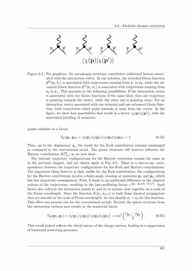
6.6. Altshuler-Aronov correction
Figure 6.4.: For graphene, the pseudospin structure contributes additional factors associ-ated with the interaction vertex. In our notation, the retarded Green functionGR(r2, r1) is associated with trajectories running from r1 to r2, while the ad-vanced Green function GA(r2, r1) is associated with trajectories running fromr2 to r1. This amounts to the following possibilities: If the interaction vertexis associated with two Green functions of the same kind, then one trajectoryis pointing towards the vertex, while the other one is pointing away. For aninteraction vertex associated with one retarded and one advanced Green func-tion, both trajectories either point towards or away from the vertex. In thefigure, we show four possibilities that result in a factor 〈χ(p)|χ(p′)〉, with theassociated labelling of momenta.
points combine to a factor
ΣF(p1,p2) = 〈χ(p1)|χ(p1)〉〈χ(p2)|χ(p2)〉 = 1. (6.54)
Thus, up to the degeneracy dg, the result for the Fock contribution remains unchangedas compared to the conventional metal. The spinor structure will however influence theHartree contribution δGH
AA, as we now show.
The relevant trajectory configurations for the Hartree correction remain the same asin the previous chapter, and are shown again in Fig. 6.5. There is a one-to-one corre-spondence between the trajectory configurations for the Fock and Hartree contributions.The important thing however is that, unlike for the Fock contribution, the configurationsfor the Hartree contribution involve a finite-angle crossing at momenta p1 and p2, whichhas two important consequences: First, it leads to an additional difference in the classicalactions of the trajectories, resulting in the fast-oscillating factor ei(p1−p2)(r1−r2)/~. Suchfactor also enforces the interaction points r1 and r2 to remain close together on a scale ofthe Fermi wavelength. Since the function K(r1, r2;ω) is built from classical propagatorsthat are smooth on the scale of Fermi wavelength, we can identify r1 = r2 for this function.This effect was present also for the conventional metals. Second, the spinor structure fromthe interaction vertices now results in the nontrivial factor
ΣH(p1,p2) = 〈χ(p1)|χ(p2)〉〈χ(p2)|χ(p1)〉 = cos2
(φp1 − φp2
2
). (6.55)
This result indeed reflects the chiral nature of the charge carriers, leading to a suppressionof backward scattering processes.
101

6. Quantum corrections to transport in graphene: a semiclassical analysis
Figure 6.5.: Configurations of trajectories that contribute to the Hartree contribution tothe Altshuler-Aronov correction. There is a one-to-one correspondence be-tween the configurations for the Hartree and the Fock contribution, Fig. 6.3.
Combining everything, the Hartree contribution can be obtained from the Fock contri-bution by the replacement
UR(r1, r2;ω)→ −dgδ(r1 − r2)〈U(p1 − p2;ω = 0)ΣH(p1,p2)〉p1,p2 (6.56)
where the factor dg comes from the existence of a closed trajectory-loop in the configura-tions of Fig. 6.5, and with the Fourier-transformed interaction
UR(q;ω) =
∫dreiqr/~UR(r;ω). (6.57)
For a short-range potential U(r1 − r2) ∝ δ(r1 − r2), we then find δGHAA = −(dg/2)δGF
AA:The spin and valley degeneracies enhance the Hartree contribution by an extra factordg = 4 compared to the Fock contribution, while chirality reduces it by a factor two[Kozi 10, Jobs 12].
Substituting the explicit expressions for the diffusion propagators, the final result forthe interaction correction to the conductivity reads
δσAA = −dge2νD
π~2
∫dω
∂
∂ω
(ω coth
ω
2T
)Im
∫d2q
(2π)2UR(q;ω)
Dq2eiωτEe−Dq2τE
(Dq2 − iω/~)3
,
(6.58)
102

6.6. Altshuler-Aronov correction
Figure 6.6.: Altshuler-Aronov correction as a function of TτE2π/~. Different curves cor-respond to different values of the interaction parameter F σ0 .
with the effective interaction kernel
UR(q;ω) = UR(q, ω)− dg〈UR(p1 − p2; 0)ΣH(p1,p2)〉p1,p2 . (6.59)
6.6.2. Coulomb interaction
The Coulomb interaction, UC(r1, r2) = e2/|r1 − r2| is long-ranged, and screening effectsneed to be incorporated into the results of the previous section. Similar to the case ofnormal metals, the structure for the result for the interaction correction remains similar,but the effective interaction kernel needs to be modified. The calculation proceeds anal-ogous to the one presented in Sec. 5.2.5, but we have to keep track on the chiral natureof particles as well as the valley degrees of freedom. The combination of spin and valleydegrees of freedom result in a total number of dg × dg = 16 channels for two-particlescattering processes. The long-range nature of the Coulomb interaction affects only thetotal singlet channel, while the remaining d2
g − 1 channels are determined by an effectiveFermi liquid parameter F σ0 (which we assume to be the same in all non-singlet channels).The value of F σ0 is also influenced by the chiral nature of the quasiparticles in graphene,as will be discussed below. For Coulomb interaction, the effectice interaction kernel forgraphene then reads
UR(q;ω) =1
dgν
~Dq2 − iω~Dq2
+ (d2g − 1)
F σ0 (~Dq2 − iω)
dgν[~Dq2(1 + F σ0 )− iω], (6.60)
which generalizes Eqs. (5.36), (5.60), and (5.61) that were obtained for normal metals.
We plot the Altshuler-Aronov correction for various values of the interaction constantF σ0 in Fig. 6.6. For small Ehrenfest time, one finds
δσAA = − e2
πh
[1 + c
(1− ln(1 + F σ0 )
F σ0
)]ln
~2πTτE
, (6.61)
103

6. Quantum corrections to transport in graphene: a semiclassical analysis
with c = d2g−1. Such an expression is well-known from diagrammatic perturbation theory
[Alts 85b], where in our case, the Ehrenfest time takes over the role of the elastic scatteringtime as a short-time cutoff. The graphene-specific physics enters the result in two ways[Kozi 10, Jobs 12]: First, the constant c = d2
g − 1 is 15 for graphene with only smoothdisorder, in contrast to c = 3 for conventional metals without valley degeneracy. Second,chirality affects the interaction constant F σ0 , as will be explained in more detail below.For small values of F σ0 , the singlet contribution is dominant in Eq. (6.61), giving rise to anegative correction to the conductance. On the other hand, for graphene, for F σ0 . −0.12,the non-singlet channels render the interaction correction positive.
For large Ehrenfest time, we find an exponential suppression
δσAA = − e2
πhe−2πTτE/~ (6.62)
where the prefactor of the exponential is determined by the singlet channel only to leadingorder in ~/TτE, hence at large Ehrenfest times, δGAA is negative and has a universalbehavior.
A striking consequence of this asymptotics is a sign-change of the interaction correctionas a function of Ehrenfest time, provided the Fermi-liquid-type interactions in the non-singlet channels are strong enough. For graphene (c = 15) this sign change already takesplace at F σ0 . −0.12, in contrast to a conventional metal (c = 3) where the sign change isobserved for F σ0 . −0.45. On the other hand, the values for F σ0 are typically somewhatsmaller in graphene, as can be seen using Thomas-Fermi approximation [Kozi 10, Jobs 12].For conventional metals, one has
F σ0 = −ν〈 2πe2?
|p1 − p2|+ κ〉p1,p2 , (6.63)
where e? is the charge screened by the substrate, and κ = 2×2πνe2? is the inverse screening
length resulting from the metal electrons (a factor 2 accounts for spin). We then find
F σ0 = −ν∫ π
0
dθ
π
2πe2?
2kF sin θ2 + 4πνe2
?
= −∫ π
0
dθ
π
α
2 sin θ2 + 2α
, (6.64)
where θ is the angle between the directions of momenta p1 and p2. We further usedkF = 2πν~vF, as well as the “effective fine structure constant” α = e2
?/~vF. The gasparameter rs is related to α as rs =
√2α. For a value rs ≈ 1 we obtain F σ0 ≈ −0.28 as a
typical size for the Fermi liquid parameter.For graphene, this calculation needs to be modified in two respects. First, the inverse
screening length is twice larger, due to the valley degree of freedom. Second, chirality con-tributes the additional factor ΣH(p1,p2) = cos2(θ/2). Both effects reduce the interactionin the non-singlet channel,
F σ0 = −∫ π
0
dθ
π
α cos2 θ2
2 sin θ2 + 4α
, (6.65)
so that now for rs ≈ 1 we find F σ0 ≈ −0.1, which is close to the transition point for asign-change as function of Ehrenfest time. The measurements of Ref. [Kozi 10, Joua 11,
104

6.7. Dephasing
Jobs 12] report F σ0 in a range between −0.05 and −0.15. However, we note that ourtheory requires graphene with a smooth disorder potential, but no other perturbations,as a necessary condition for the value c = 15 in Eq. (6.61), since there are 16 diffusionchannels. Trigonal warping or ripples, while not invalidating the semiclassical analysis,reduce the number of diffusive channels to 8, resulting in a prefactor c = 7. In case of strongintervalley scattering, only four diffusion modes are present resulting in a prefactor c = 3(see Ref. [Kech 08, Khar 08]) — although in that case the conditions for the semiclassicalanalysis are no longer valid. The aforementioned experiments on interaction correctionsreport to be in a regime where c = 3 or c = 7.
6.7. Dephasing
We now turn to the second type of interaction correction, responsible for the dephasing.The way of calculating the dephasing in this section follows that of Ref. [Alts 82]. Analternative discussion based on perturbation theory, similar to that of the previous Section,is given in the appendix.
Because of the interactions, the electrons are subject to a time-dependent potentialV (r, t). This potential affects the phase that electrons accumulate while propagatingthrough the sample. These phase fluctuations can be included into the classical actionSα of the trajectory α as it appears in the semiclassical expression (6.4) for the Greenfunction by the substitution
Sα → Sα + δSα(t), (6.66)
where the correction δSα(t) depends on the time t at which the electron exits the sample.The shift reads [Alts 82, Altl 07]
δSα(t) =
∫ t
t−ταdt′V [rα(t′), t′], (6.67)
where τα is the duration of the trajectory α.Such a shift of the classical actions does not affect the Drude conductivity, because
the actions from the “retarded” and “advanced” trajectories cancel. It does, however,affect the weak antilocalization correction. Equation (6.42) acquires an additional factorei(δSα(t)−δSβ(t)) which, when averaged over the time t, reduces the contribution from thetrajectory pair α, β by a factor⟨
ei(δSα(t)−δSβ(t))/~⟩t
= e−(1/2~2)〈(δSα(t)−δSβ(t))2〉t . (6.68)
The time average can be calculated using the quantum fluctuation-dissipation theorem,
〈V (r, t)V (r′, t′)〉 =
∫d2qdω
(2π)3
ω
2T sinh2(ω/2T )eiq·(r−r
′)−iω(t−t′)ImUR(q, ω),
which gives
1
2〈((δSα(t)− δSβ(t))2〉t =
∫ τα
0dt1
∫ t1
0dt2
∫d2qdω
(2π)3
ω
2T sinh2(ω/2T )ImUR(q, ω)
× Re[e−iω(t1−t2)
(eiq·rα(t1) − eiq·rβ(t1)
)(e−iq·rα(t2) − e−iq·rβ(t2)
)]. (6.69)
105

6. Quantum corrections to transport in graphene: a semiclassical analysis
(Note that τα = τβ for the trajectory pairs that contribute to weak antilocalization.)One immediately concludes that for the trajectories α and β that contribute to the weakantilocalization correction δGWAL only points rα or rβ in the loop or encounter segmentsof Fig. 6.1 contribute to 〈((δSα(t)− δSβ(t))2〉t.
To find an explicit expression for the dephasing correction in the limit of weak dephasing,we expand the correction factor (6.68) to lowest order in the interaction UR(q, ω) andcalculate the leading interaction correction δGdeph to the weak antilocalization correctionδGWAL. We consider contributions from positions rα,β(t1) and rα,β(t2) in the loop andencounter regions separately.
The calculation for the dephasing in the loop segment is very similar to the one carriedout in standard diagrammatic perturbation theory. The discussion below closely followsthat of Ref. [Marq 07]. With both positions rα,β(t1,2) in the loop region, see Fig. 6.7, wefind that dephasing in the loop segment leads to the replacement P (r′, r′; t)→ P (r′, r′; t)+δP (r′, r′; t) for the loop propagator in Eq. (6.47), with
δP (r′, r′; t) =− 4
~2
∫dq
(2π)2
∫dω
2π
ω ImUR(q;ω)
2T sinh2(ω/2T )
×∫ t
0dt1
∫ min(t1,t−t1)
0dt2 cos[ω(t1 − t2)/~]
× [Pq(t2, t1 − t2, t− t1)− Pq(t2, t− t1 − t2, t1)] , (6.70)
where
Pq(τ1, τ2, τ3) =
∫dr1dr2 cos[q · (r1 − r2)]P (r′, r2, τ3)P (r2, r1, τ2)P (r1, r
′, τ1). (6.71)
Inserting the diffusion propagator P (q, τ) = e−Dq2τ , one finds
Pq(τ1, τ2, τ3) = P (r′, r′; t)e−Dq2τ2(1−τ2/t), (6.72)
with t = τ1+τ2+τ3. After insertion of the interaction (6.60) and evaluation of the integralsover time, frequency, and momentum in Eq. (6.70) (see Appendix D.3), one finds
δP (r′, r′; t)
P (r′, r′; t)= −αtT
~g0lntT
~, (6.73)
with the dimensionless conductance g0 = 2π~dgνD, and the constant
α = 1 + (d2g − 1)
(F σ0 )2
(1 + F σ0 ) (2 + F σ0 ). (6.74)
This result signifies that at large times the loop propagator gets suppressed by in-teractions. Here we calculated the leading order correction, describing the onset of anexponential suppression. (In fact, in two dimensions the decay is not purely exponential[Marq 07], but contains an additional logarithm e−at ln t, as can be seen from Eq. (6.73)).We estimate the dephasing rate as the time when the leading correction becomes unity,i.e.,
1
τ loopϕ
' αT
g0~lng0
α. (6.75)
106

6.7. Dephasing
Figure 6.7.: Dephasing in the loop segment: for the calculation of the lowest-order in-teraction correction the propagation around the loop is split into three seg-ments r′ → r1 (duration τ1), r1 → r2 (duration τ2), and r2 → r′ (durationτ3). For our figure, the trajectories α (solid) and β (dashed) are travelledin clockwise and counterclockwise direction, respectively. The left diagramrepresents the contribution from the term proportional to eiq·rα(t1)−iq·rα(t2)
in Eq. (6.69); the right diagram represents the contribution from the termproportional eiq·rβ(t1)−iq·rα(t2). The remaining two contributions, from termsproportional to eiq·rα(t1)−iq·rβ(t2) and eiq·rβ(t1)−iq·rβ(t2) are not shown. Thefigures have been drawn for the case that 0 < t2 < min(t1, t − t1), which isthe domain of integration in Eq. (6.70).
The leading logarithmic dependence in this expression agrees with that obtained in Ref.[Naro 02] for a standard two-dimensional electron gas (dg = 2).
We now turn to the encounter region, where dephasing leads to an additional suppres-sion of weak antilocalization, if the typical time for the encounter passage, the Ehrenfesttime τE, is sufficiently long. As discussed before, dephasing is ineffective, as long as thetrajectories coincide. Within the encounter region, the trajectories α and β are separatedby a small distance, which does not exceed the classical correlation scale Lc. Dephasingthen only plays a role for interaction that transfers a momentum larger than inverse meanfree path, and therefore can resolve such small distance [Altl 07, Peti 07, Whit 08]. Onthe other hand, for low temperatures Tτ 1 one has ωτ 1. In this limit, the imaginarypart of the screened interaction reads [Zala 01]
ImUR(q;ω) = − βω
qdg~νvF, (6.76)
where ν = kF/2π~vF is the density of states and we abbreviated
β = 1 + (d2g − 1)
(F σ0 )2
(1 + F σ0 )2 . (6.77)
Note that ImUR(q;ω) is proportional to q−1, which is different from the dependenceImUR(q;ω) ∝ q−2 of the diffusive limit. This difference will result a different T -dependenceof the dephasing rate in comparison to the loop contribution [Altl 07].
We proceed by the integration over ω, which can be done explicitly using the known ω
107

6. Quantum corrections to transport in graphene: a semiclassical analysis
dependence of ImUR(q;ω) [Marq 07],∫dω
2π
ω2e−iω(t1−t2)/~
2T sinh2(ω/2T )= 2πT 2w[πT (t1 − t2)/~]. (6.78)
Here the function w(x) = (x cothx − 1)/ sinh2 x is peaked around x = 0, normalized∫∞−∞ dxw(x) = 1, and w(0) = 1/3. Hence, the times t1 and t2 need to be close together
on the scale of inverse temperature. On the other hand, dephasing sets in on timesmuch larger than T−1, as we will show below. In the following, we therefore may assumethat |t1 − t2| τE, when we consider encounters that are long enough to be affected bydephasing. (In fact, the calculation below will show that the main contribution stems fromtime differences |t1 − t2| much smaller than the elastic mean free time.) In particular thisamounts to consider the effect of interaction during the first and second passage throughthe encounter separately, since they are separated by a loop of long duration. The sameobservation also allows us to neglect contributions where t1 is in the encounter, whereas t2is in the loop or vice versa. We therefore focus on the first passage through the encounterregion, where the trajectories α and β are separated by a distance d(t) = rβ(t) − rα(t),with the magnitude
d(t) ' λF eλt, (6.79)
where t is varying form 0 to τE. We can use this to rewrite the last two factors of Eq.(6.69) as
(eiq·rα(t1) − eiq·rβ(t1))(e−iq·rα(t2) − e−iq·rβ(t2))
= 4eiq·[r(t1)−r(t2)] sin[q · d(t1)/2] sin[q · d(t2)/2], (6.80)
where r(t) = [rα(t) + rβ(t)]/2 represents a trajectory intermediate between α and β.After performing the average over disorder configurations, we find that inclusion of the
leading-order dephasing correction amounts to the replacement P (r′, r; τE)→ P (r′, r; τE)+2δP (r′, r; τE) in Eq. (6.47), where the factor two accounts for the two passages throughthe encounter region, with
δP (r′, r; τE) =− 8πT 2β
~3vFdgν
∫d2q
(2π)2
1
q
∫ τE
0dt1
∫ t1
0dt2w(πT (t1 − t2)/~)
× Pencq (t1, t2, τE − t1 − t2) sin[q · d(t1)/2] sin[q · d(t2)/2] (6.81)
and
Pencq (t1, t2, τE − t1 − t2) =
∫dr1dr2 cos[q · (r1 − r2)]
× P (r′, r2, τE − t1)P (r2, r1, t1 − t2)P (r1, r, t2), (6.82)
see Fig. 6.8. Because of the smallness of |t1 − t2|, the propagator P (r2, r1, t1 − t2) is theballistic propagator, whereas the propagators P (r′, r2, τE−t1) and P (r1, r, t2) can be takenin the diffusion approximation. We change the integration variables to the mean time tand the difference time t = t1− t2. Again using the smallness of |t1− t2|, we replace d(t1)and d(t2) by d(t). We neglect correlations between d(t) and the direction of the velocity
108

6.7. Dephasing
Figure 6.8.: Dephasing in the encounter segment: For the calculation, the encounter issplit into three segments r′ → r1 (duration τ1 = t2), r1 → r2 (durationτ2 = t1 − t2), and r2 → r′ (duration τ3 = τE − t2). Only configurations inwhich |t1 − t2| τE contribute to the interaction correction δGdeph. In themiddle segment, the distance between the trajectories α and β is d(t) = λFe
λt,where t = (t1 + t2)/2. The figure has been drawn for the case 0 < t2 < t1,which is the domain of integration in Eq. (6.81)
at time t. Using P (r1, r, t2) ' P (r2, r, t1), again because of the smallness of |t1 − t2|, wefind
Pencq (t1, t2, τE − t1 − t2) ' P (r′, r; τE)J0(vFq|t|), (6.83)
where we inserted the Fourier transform of the ballistic propagator. Since the integrationover t converges for |t| ∼ 1/vFq, the argument of the function w may be set to zero in Eq.(6.81). Finally, the angular average over the direction of d(t) gives a factor 1− J0(qd(t)),so that we find
δP (r′, r; τE) = − 4πT 2β
3~3v2Fdgν
P (r′, r; τE)
∫d2q
(2π)2
1
q2
∫ τE
0dt [1− J0 (qd(t))] , (6.84)
We cut off the logarithmic divergence of the q integration at large q at λ−1F , which gives
δP (r′, r; τE) = − 2T 2β
3~3v2Fdgν
P (r′, r; τE)
∫ τE
0dt ln
d(t)
λF.
The remaining time-integration is easily evaluated with the help of Eqs. (6.79), (6.41),and we obtain ∫ τE
0dt ln
d(t)
λF=τE
2lnLc
λF. (6.85)
Hence, our the final result reads
δP (r′, r; τE)
P (r′, r, τE)= − T 2βτE
3~3v2Fdgν
lnLc
λF. (6.86)
One may identify the right-hand side of Eq. (6.86) with τE/τencϕ , where τ enc
ϕ is an effectivedephasing time for the encounter region. With this identification, Eq. (6.86) describesthe onset of an exponential suppression of the weak localization ∝ e−2τE/τ
encϕ at large
Ehrenfest times. Note that the time τ encϕ is twice the dephasing time τball
ϕ that one finds
109

6. Quantum corrections to transport in graphene: a semiclassical analysis
from dephasing in the loop region in the ballistic regime [Naro 02], consistent with thetheory of Ref. [Altl 07]. [To compare with Ref. [Naro 02], take the energy-dependentdephasing time τϕ(ε) from Eqs. (18) and (19a) of Ref. [Naro 02] in the limit Tτ ~ andcalculate (τball
ϕ )−1 =∫dε (−∂f/∂ε) τϕ(ε)−1 with, for a conventional metal, dg = 2. The
low-momentum cut-off in Ref. [Naro 02] is the inverse mean free path, whereas it is theclassical correlation length Lc in our case. The two lengths need not be equal, see Eq.(6.17).]
6.8. Conclusion
In this chapter we have presented a trajectory-based semiclassical theory of the quan-tum corrections to transport in graphene in the presence of a random potential that issmooth on the scale of the Fermi wavelength. A prominent role is played by the Ehrenfesttime, which serves as a short-time threshold for the appearance of quantum interferenceeffects. The Ehrenfest time also plays an important role for electrons in a conventionaltwo-dimensional electron gas (with quadratic dispersion) if they are subject to a smoothrandom potential.
Compared to the conventional case, charge carriers in graphene have an additionalpseudospin degree of freedom and they have an additional valley degeneracy, which leadsto a few subtle modifications of the quantum corrections with respect to the conventionalcase. The pseudospin vector always points along the direction of motion, reflecting thechiral nature of the charge carriers in graphene. The evolution of the pseudospin along thetrajectory is associated with a Berry phase of the spin transport, that additionally entersthe semiclassical Green function. This Berry phase is responsible for a sign change inthe weak localization correction, giving antilocalization behavior. The presence of a finiteEhrenfest time reduces the magnitude of this correction, but with a multiplicative factorthat is the same for weak localization and weak antilocalization. We also considered thesuppression of weak (anti)localization from dephasing at finite temperatures, and identifiedthere, too, the role of the Ehrenfest time.
For the interaction correction there are two important differences with the case of theconventional two-dimensional electron gas: The Hartree-type processes (or, more precisely,interaction non-singlet channels) contain an additional angular dependence, as a result ofchirality. Moreover, importance of screening is changed, because of the presence of thevalley degeneracy. A finite Ehrenfest time suppresses the Altshuler-Aronov correction,in a similar way as for conventional metals, but unlike for weak (anti)localization thesuppression is not simply a multiplicative factor. Interestingly, the interaction correctionmay undergo a sign change as a function of Ehrenfest time, for sufficiently strong inter-action in the non-singlet channels. For graphene, the interaction strength at which thissign change takes place is smaller than in conventional electron gases, which may place itwithin experimental reach, as discussed in Sec. 6.6.
110

7. Conclusion
Graphene has stimulated a great deal of attraction in solid state physics in recent years. Itsspecial electronic properties arise from a quasi-relativistic dispersion, that is characteristicfor the honeycomb lattice formed by the atoms of a single layer of graphite. The relativisticnature of the electronic excitations in graphene gives rise to series of unconventional effects,that are observed in studies of the transport properties of graphene. In this thesis, wediscussed various aspects of such unusual features in the electronic properties of graphene,and their relation to the peculiar bandstructure.
One part of the thesis discussed the possibility of electrostatic confinement in graphene.While it is common, to restrict the electronic motion to a quantum dot with the help pfmetallic gates in semiconductor structures, such procedure is problematic in graphene, dueto the absence of a bandgap. The best option to create quantum dots in graphene consistsof a doped region that is surrounded by an an undoped graphene structure, where theFermi level lies at the Dirac point. Although the density of states vanishes in the regionoutside of the dot, Klein tunneling opens a way to exit the dot, as electrons approachingthe surface of the dot under normal incidence will be transmitted with unit probability. Onthe other hand, electrons that hit the surface away from normal incidence will be reflectedback and remain inside the dot. Such angle-specific scattering suggests, that electrostaticconfinement should be possible for certain geometries, that exclude normal incidence.
One way to obtain information about possible confinement in graphene, is to attach thequantum dot surrounded by undoped graphene to source and drain contacts and studythe two-terminal conductance. The spatial restriction of electronic motion gives rise todiscrete levels of the quantum dot, that are observed as resonances in the conductance. Thestructure of the resonances, as well as their behavior upon changing the coupling betweendot and leads contains information about the nature of the electronic bound state and thedegree of confinement. As prototypical examples, we studied a circular quantum dot withintegrable classical dynamics, that should support bound states according to the argumentsgiven above, and a stadium-shaped quantum dot, which should lack confinement in viewof the classical chaotic motion.
Previous numerical studies indeed found sharp resonances for a circular graphene quan-tum dot, that correspond to well-confined states, while for the chaotic structure the res-onances are typically broad. Further improvement has been made by linking the conduc-tance to the scattering matrix of the quantum dot, which allows for an analytic solutionfor the circular quantum dot. In this thesis, we extended this machinery, in order to beable to calculate the conductance of a quantum dot of generic shape from its scatteringmatrix. In this way, we have been able to extract information about the structure of thebound states from the lineshape of the resonant features in the conductance. Moreover, wecould easily scale to the important limit of weak coupling between dot and leads, for whichthe resonances become isolated. Here, we could make the distinction between features of
111

7. Conclusion
a regular and a chaotic dot shape rigorous, since the width of the resonances is shrinkinglinearly in the ratio of dot size vs. distance to the leads for a chaotic dot upon weakeningthe coupling to the leads, while the regular dot contains resonances that shrink at a higherpower, and therefore possess a higher degree of confinement.
Remarkably, the resonances for the chaotic structure persist at a finite height close to theconductance quantum even in the limit of arbitrarily small coupling to the leads. In thisthesis, we identified the Berry phase, that occurs in graphene from the pseudospin whichindicates the sublattice structure, as the origin of such effect. Upon a circular motion of theelectron, the pseudospin winds once around its axis, being responsible for an accumulationof a phase of π in the electronic wavefunction. The Berry phase is also responsible for aquantization of the angular momentum to half-integer multiples of ~. We could isolate thesignificance of such phase on possible confinement in graphene by adding an additionalflux tube to the system, which contains half a flux quantum. Electrons encircling suchflux tube acquire an Aharonov-Bohm phase of π, which is precisely cancelling the effect ofa Berry phase. For this situation, the kinematic angular momentum, which is relevant forthe classical argumentation, is shifted to integer values, where the state with zero angularmomentum cannot be confined by means of gate potentials. Such state hence correspondsto normal incidence on the surface, where Klein tunneling prohibits confinement. Indeedwe found a clear distinction between regular and chaotic shapes of the dot in the presenceof the flux tube, where bound states are now only found in regular structures.
An alternative route to access information about the degree of confinement in differentquantum dots is to investigate the density of states, that can also be inferred from thescattering matrix of the quantum dot. We showed, that such type of calculation pro-vides an effective method to gain information about resonant levels of the dot, and wediscussed in this thesis, how the different scenarios of quantum dots in graphene give riseto discernable features in the density of states.
To sum up, we have been able to derive a conclusive picture about which effects in-fluence the electrostatic confinement in graphene. We remark, that the question if it ispossible to confine electrons in graphene with metallic gates could not be answered a prioribased on intuition, but demanded a careful study that revealed some surprising insightsin the unusual Dirac physics in graphene. We believe, that the methods developed withinthis thesis in this context, offer valuable tools for the study of related problems. As anexample, we would like to mention a possible charge trapping when the graphene sheetis deformed, for example externally with a scanning tunneling microscope tip. Electronsmoving through the deformed graphene layer are affected by an effective magnetic field,that maybe able to localize the electrons. Another direction would be to drive the systemout of equilibrium by changing the gate voltage of the quantum dot (or the height ofthe deformation of the graphene sheet) in time. Nonequilibrium phenomena are typicallyaccompanied by rich physical effects, therefore it might be worth to extend the methodsdeveloped in this thesis and include a time-dependence.
In this thesis, we further employed semiclassical methods in order to study quantumeffects in transport in disordered metals. The wave nature of electrons is confirmed by anumber of features in electronic transport, such as weak localization, or the interactioncorrection to the conductivity. For a system where the disorder is changing on a scalemuch larger than the Fermi wavelength, which describes the typical extension of an elec-
112

tronic wavepacket, the electronic motion is governed by classical dynamics. The essenceof semiclassical methods in quantum transport is to calculate quantum effects to the con-ductivity based on classical trajectories through the conductor – quantum effects arisefrom the interference of different trajectories. The semiclassical limit is characterized bythe appearence of an additional timescale, the Ehrenfest time, not present for short-rangequantum disorder, which essentially serves as a short-time threshold for the occurence ofinterference effects.
One of the projects of this thesis contained the semiclassical analysis of the interactioncorrection to the conductance. Our study extended a previous investigation that deriveda semiclassical theory for the interaction correction of a ballistic double quantum dot, thesimplest system for which interaction corrections can occur. The study presented in thisthesis is capable to treat a generic type of conductor that gives rise to classical electronicdynamics and allows for both short and long range type of interaction. In particular, weaddress the interaction correction to the conductance of antidot arrays, an experimentallyrelevant example for a system where electrons are following classical trajectories. We findthat the Ehrenfest time is acting as a short-time threshold for the occurrence of the in-teraction correction, and consequently the interaction correction is strongly suppressed,once the Ehrenfest time exceeds the dwell time or inverse temperature. The sensitivityto temperature is special to the interaction correction, and maybe of importance for ex-perimental studies, where temperature provides a well-adjustable quantity. For Coulombinteraction, there is a competition between Hartree and Fock type contributions to theconductance, which come with opposite sign. This competition may lead to a sign changeof the interaction correction, as one varies Ehrenfest time, if the interaction is strongenough.
We further studied quantum corrections to transport in graphene in this thesis, based onsemiclassical approximations. For the semiclassical limit to hold true, we require graphenethat is doped away from the Dirac point, and subject to a smooth disorder potential,which may occur in graphene samples that are placed on a substrate with high dielectricconstant. The semiclassical theory for graphene differs from the theory for conventionalmetals by the existence of the pseudospin, which modifies the semiclassical propagator forthe electrons, such that it contains information also about the transport of the pseudospin.In this thesis, we discussed weak localization, and the interaction corrections, specificallythe Altshuler-Aronov correction and dephasing, for graphene from a semiclassical point ofview, based on classical trajectories. For weak localization, the Berry phase associated withthe pseudospin is responsible for a change from weak localization to weak antilocalization.We also discussed quantitatively, how such effect is suppressed by a finite Ehrenfest time.For the interaction correction, the pseudospin together with the additional valley degreeof freedom is influencing the magnitude of the interaction correction. Interestingly, thesign change as a function of Ehrenfest time mentioned before appears within experimentalreach for graphene.
Summarizing, in this thesis we further extended the range of applicability of semiclassicalmethods for the calculation of quantum transport. The usage of semiclassical methodsprovides several advances, it combines the highly intuitive language based on classicaltrajectories together with a powerful quantitative method to calculate the magnitude ofthe quantum corrections, and it can deal with the appearence of the Ehrenfest time in
113

7. Conclusion
systems with smooth “classical” disorder. We are optimistic that the developments ofthis thesis are useful for a further extension of the semiclassical methods to other areas inquantum transport, for instance in superconducting systems.
114

Appendix


A. Appendix to Chapter 3
A.1. Matrix Green Function
In this appendix, we give explicit expressions for some of the matrix Green functionappearing in Sec. 3.3. We follow the supplementary material of Ref. [Tito 10], but ourresults for the d-wave channel go beyond that reference.
Using Pauli matrices τx, τy, and τz for the retarded-advanced (RA) degree of freedom,and with τ0 for the 2 × 2 unit matrix in the RA grading, the explicit expression for thematrix Green function G0 is
G0(x, x′; y) =1
4~vLV (x)ΛΛτ ΛσΛV −1(x′) (A.1)
with Λ =
(1 00 0
)⊗ σz +
(0 00 1
)⊗ σ0 and
Λτ =
(i cosh(φy/2L) sinh(φy/2L)sinh(φy/2L) −i cosh(φy/2L)
)⊗ σ0, (A.2)
Λσ = τ0 ⊗
(1
sin[π(x+x′+iy)/2L]1
sin[π(x−x′+iy)/2L]1
sin[π(x−x′−iy)/2L1
sin[π(x+x′−iy)/2L
), (A.3)
V (x) =
(sin φ(L−x)
2L cos φ(L−x)2L
i cos φx2L i sin φx2L
)⊗ σ0. (A.4)
Ths s-wave contribution of the regularized Green function can be found as
Gssreg(x0) = limx′→x0y→0
[G0(x0, x′; y)− g(x0 − x′, y)]
=i
4~vLV (x0)
(1
sin(πx0/L) −σxφ/πσxφ/π − 1
sin(πx0/L)
)V −1(x0) (A.5)
Contributions from higher angular momentum modes are obtained by keeping higher termsof the Taylor series. Therefore, we write the regularized Green function as
Greg(r, r′) =∑µ,ν
1
µ!
1
ν![(r− r0)
−→∇ ]µGreg(r0, r0)[
←−∇ ′(r′ − r0)]ν (A.6)
Here,−→∇ acts to the right, on the first argument of the Green function, and
←−∇ ′ acts to the
left, on the second argument of the Green function. We can simplify this expression byusing the equations of motion of the regularized Green function,
− iσ−→∇Greg = 0, Greg(−i
←−∇ ′σ) = 0 (A.7)
117

A. Appendix to Chapter 3
from which immediately follows, that
∂yGreg(r, r′) = iσz∂xGreg(r, r′), ∂y′Greg(r, r′) = ∂x′Greg(r, r′)(−iσz). (A.8)
This enables us to rewrite Eq. (A.6) as
Greg(r, r′) =∑µ,ν
1µ! [(x− x0) + iσz(y − y0)]µGµνreg
1ν! [(x
′ − x0)− iσz(y′ − y0)]ν , (A.9)
with
Gµνreg = ∂µx∂νx′Greg(r0, r0). (A.10)
We now give the explicit expressions for Gµνreg up to d-wave order. In order to keep theexpressions short, we focus on the case, where the dot is placed in the middle of the sample(x0 = L/2),
Gsp/psreg =i
8~vL2V (x0)
(±π2−3φ2
6π σx −φ−φ ±π2−3φ2
6π σx
)V −1(x0),
Gppreg =i
16~vL3(π2 − φ2)V (x0)
(1 φ
3πσx− φ
3πσx −1
)V −1(x0),
Gsd/dsreg =i
16~vL3(π2 − φ2)V (x0)
(1 − φ
3πσxφ3πσx −1
)V −1(x0),
Gpd/dpreg =i
32~vL4V (x0)
(∓7π4−30π2φ2+15φ4
60π σx φ(−3π2 + φ2)
φ(−3π2 + φ2) ∓7π4−30π2φ2+15φ4
60π σx
)V −1(x0),
Gddreg =i
64~vL5V (x0)
(5π4 − 6π2φ2 + φ4 φ−7π4+10π2φ2−3φ4
15π σx
−φ−7π4+10π2φ2−3φ4
15π σx −(5π4 − 6π2φ2 + φ4)
)V −1(x0).
The element Gssreg is given by Eq. (A.5). Since V (x0) has no matrix structure in pseudospinspace, it commutes with the T -matrix, and therefore does not play a role for the generatingfunction.
Upon inserting (A.9) into the generating function (Eq. (3.21)), we find
δF = ln det[1−TGreg], (A.11)
where Greg is a (infinite) matrix with entries Gµνreg (µ,ν = 0, 1, ...) and the matrix Tcontains the elements Tµν
Tµν =
∫d2rd2r′ 1
µ! [(x− x0)− iσz(y − y0)]µT (r, r′) 1ν! [(x
′ − x0) + iσz(y′ − y0)]ν . (A.12)
This is Eq. (3.23) of the main text. In the limit that the size R of the quantum dot ismuch smaller than L, this expansion is convergent, and it is a good approximation to limitthe number of angular momentum “channels” involved in the expansion. In the simplestcase, one takes into account the s-wave contribution µ = ν = 0 only. This limit wasconsidered in Ref. [Tito 10]. The accuracy can be improved by including contributions
118

A.1. Matrix Green Function
from higher angular momentum. The expressions derived above allow one to go up to thed-wave contribution.
In order to relate the object Tµν of Eqs. (3.23) or (A.12) to the T matrix in the partial-wave expansion, it is instructive to compare the plane-wave and circular-wave basis setsof eigenstates of the free Dirac Hamiltonian H0 = −iσ∇. The plane wave basis consistsof eigenstates, which are labeled by their wavevector k = (k cos θk, k sin θk),
ψk(r) =eikr√
2
(1eiθk
). (A.13)
Here and below, we restrict ourselves to positive energy solutions (conduction band) only.In the implementation, this can be achieved by choosing the gate potential of the dot tobe negative. The circular-wave states are combined eigenstates of the Hamiltonian andthe total angular momentum Lz + 1
2σz, and are therefore labeled by their wavenumber kand their half-integer angular momentum quantum number m,
ψkm(r) =
√k
4πeimθ
e−iθ2J|m− 1
2 |(kr)
eiθ2 isgn(m)J|m+ 1
2 |(kr)
. (A.14)
Here, Jν is the Bessel function of ν-th order. The 2 × 2 matrix Ψkµ of the main text isrelated to the ψkm as Ψkµ = (ψk,µ+1/2, iψk,−µ−1/2). The basis change between plane wavesand circular waves is expressed through the equation
ψk(r) =
√2π
k
∑m
i|m−12|e−i(m−
12
)θkψkm(r). (A.15)
For the scattering problem in the infinite graphene sheet, we place the center of thequantum dot at the origin. We may express the T -matrix in the plane-wave basis throughthe T -matrix in real space as
T (k,k′) =1
2
∫d2rd2r′(1 e−iθk)T (r, r′)
(1
eiθ′k
)× exp[ik(x′ cos θ′k + y′ sin θ′k − x cos θk − y sin θk)]. (A.16)
On the other hand, the same matrix elements can be also written in spherical wave basis,
T (k,k′) =2π
k
∑nm
(−i)|n−12|i|m−
12|ei(n−
12
)θke−i(m−12
)θ′kTnm(k) (A.17)
The partial-wave T matrices Tmn introduced here and Tµν of the main text are related as
Tµν =
(Tµ+1/2,ν+1/2 iTµ+1/2,−ν−1/2
−iT−µ−1/2,ν+1/2 T−µ−1/2,−ν−1/2
). (A.18)
Comparing Eqs. (A.16) and (A.17), we obtain a relation between the T -matrix in sphericalwave basis and the T -matrix in real space. For example, for the s-wave channel we find
2π
k
(T 1
2, 12(k) iT 1
2,− 1
2(k)
−iT− 12, 12(k) T− 1
2,− 1
2(k)
)=
1
2
∫d2rd2r′T (r, r′) +O(k), (A.19)
119

A. Appendix to Chapter 3
so that
T 00 = limk→0
4π
k
(T 1
2, 12(k) iT 1
2,− 1
2(k)
−iT− 12, 12(k) T− 1
2,− 1
2(k)
)= lim
k→0
4π
kT00(k), (A.20)
where, in the last equation, we used the 2 × 2 matrix notation with integer indices usedin the main text. The remaining identities in Eq. (3.25) follow similarly.
A.2. Low-k-Limit of Scattering matrix
In this appendix, we present the details how to determine the low-k limit of the scatteringmatrix. As explained in the main text, we modify the scattering problem, such that wesolve the scattering problem for particles with wavenumber k1 = k + k′ in the potentialU ′ = U +~k′v. We then need to relate the scattering matrix S′ for this problem, in whichU ′ is set to zero outside a certain cut-off radius a to the scattering matrix S for the originalproblem, in which U , not U ′ is set to zero for r > a.
In order to relate these two scattering matrices, we need to calculate the scatteringmatrix of a potential step, in which the potential is zero for r > a and equal to u = ~k′vfor r < a. Hereto, we expand the wavefunctions for r < a and r > a in terms of incomingand outgoing circular waves with wavenumber k′ + k and k, respectively,
ψa−(r) =∑m
(L+mψk+k′,m,+(r) + L−mψk+k′,m,−(r)),
ψa+(r) =∑m
(R+mψk,m,+(r) +R−mψk,m,−(r)), (A.21)
where the scattering states ψk,m,± are obtained from the basis states ψkm in Eq. (A.14)by the replacement J(kr) → H±(kr). The coefficients R±m and L±m are related throughthe transfer matrix T , (
R+m
R−m
)= Tm(k, k + k′, a)
(L+m
L−m
), (A.22)
which is easily calculated from continuity of the wave function at r = a,
Tm(k, k + k′, a) =πa
4iTm(k, k + k′, a)
√k(k + k′), (A.23)
where the 2× 2 matrix Tm(k, k + k′, a) has entries
Tm(k, k + k′, a)11 = H(−)
|m|+ 12
(ka)H(+)
|m|− 12
(ka+ k′a)−H(−)
|m|− 12
(ka)H(+)
|m|+ 12
(ka+ k′a),
Tm(k, k + k′, a)12 = H(−)
|m|+ 12
(ka)H(−)
|m|− 12
(ka+ k′a)−H(−)
|m|− 12
(ka)H(−)
|m|+ 12
(ka+ k′a).
(A.24)
The other entries are given by the relations Tm(k, k + k′, a)21 = −Tm(k, k + k′, a)∗12,Tm(k, k + k′, a0)22 = −Tm(k, k + k′, a)∗11. The transfer matrix is converted into reflec-
120

A.2. Low-k-Limit of Scattering matrix
tion/transmission coefficients using the standard relations
ρ = T12(T22)−1,
τ = (T22)−1,
τ ′ = T11 − T12(T22)−1T21,
ρ′ = −(T22)−1T21. (A.25)
Upon taking the limit k → 0, we find
ρm = 1 +iπa2|m|
[(|m| − 12)!]222|m|−1
H(−)
|m|+ 12
(k′a)
H(−)
|m|− 12
(k′a)k2|m| +O(k2|m|+1),
τm = τ ′m =1
(|m| − 12)!2|m|−
32
a|m|−12
√k′
1
H(−)
|m|− 12
(k′a)k|m| +O(k|m|+1),
ρ′m = −H
(+)
|m|− 12
(k′a)
H(−)
|m|− 12
(k′a)+O(k). (A.26)
We can now relate the scattering matrices S′ for particles with energy k′ in the potentialU ′ = U + ~k′v and U ′ = 0 for r > a to the scattering matrix S for particles with energyk in the potential U , with U = 0 for r > a,
S = ρ+ τ ′(1− S′ρ′)−1S′τ. (A.27)
Inserting the above expansions, we get an expression of the form
Snm(k) = δnm + S(1)nm k
|n|+|m| +O(k|n|+|m|+1), (A.28)
coinciding with Eq. (3.33) in the main text. The coefficient S(1) depends on a, k′ and S′.
121

B. Appendix to Chapter 4
B.1. Numerical simulation of the two-terminal transport
The numerical approach for the two-terminal transport in the presence of a π-flux followsRef. [Bard 07]. The potential V (r) is replaced by a potential
∑n Vn(y)δ(x − xn) that is
nonzero at N discrete values −L/2 = x0 < x1 < x2 < . . . < xN−1 < xN = L/2 of the xcoordinate, with
Vn(y) =
∫ (xn+xn+1)/2
(xn−1+xn)/2dxV (x, y), n = 1, 2, . . . , N − 1.
Between the discrete points the wavefunction is solved from the free Dirac equation. Thissolution takes its simplest form after Fourier transform with respect to the transversecoordinate y, because the free Dirac equation does not couple different transverse modes.These solutions are then matched by applying the appropriate boundary conditions atthe discrete points x = xj , j = 1, 2, . . . , N . A numerically stable method to implementthis program is to express both the solution of the free Dirac equation and the matchingconditions at the discrete points x = xj in terms of scattering matrices. The scatteringmatrix of the entire sample is then obtained from convolution of the scattering matricesof the 2N − 1 individual components. The result of the calculation is the transmissionmatrix t, which is related to the two-terminal conductance via the Landauer formula,
G =4e2
htr tt†, (B.1)
where the trace is taken of the transverse Fourier modes. The number of “slices” N andthe number of transverse modes M must be chosen large enough, that the conductance Gno longer depends on N and M .
The vector potential (4.15) corresponds to the boundary condition
limx↑0
ψ(x, y) = − limx↓0
ψ(x, y) for −W/2 < y < 0, (B.2)
whereas ψ(x, y) is continuous at x = 0 for 0 < y < W/2. In the approach described above,this boundary condition is expressed in terms of a scattering matrix relating incoming andoutgoing waves at x ↑ 0 and x ↓ 0. This scattering matrix has no reflective part, whereasthe transmission matrix is
tmn =
0 if m− n even,−4i/[(km − kn)W ] if m− n odd,
(B.3)
where the integers m and n label the transverse modes and kn = 2πn/W . This transmis-sion matrix has the special properties that t = t† and t2 = 1.
123

B. Appendix to Chapter 4
In order to ensure numerical stability, unitarity must be preserved while restricting toa finite number of transverse modes M . For the transmission matrix (B.3) this can beachieved using the following trick: One first builds the hermitian matrix h = i(eiφ −t)/(t + eiφ) = cotφ − t/ sinφ out of the transmission matrix, where φ is a phase thatcan be chosen arbitrarily, then truncates h, which can be done straightforwardly withoutcompromising hermiticity, and then uses the inverse relation t = eiφ(1 + ih)/(1 − ih)to obtain a finite-dimensional transmission matrix. In our numerical calculation we setφ = π/2. We verified that the elements of the resulting finite-dimensional transmissionmatrix approach the elements of the exact transmission matrix (B.3) in the limit that thenumber of transverse mode M →∞.
B.2. Numerical simulation of the density of states
In this appendix, we provide details concerning the numerical calculation of the densityof states out of the scattering matrix for a gate-defined dot or arbitrary shape. We firstchoose a disc of radius R that fully covers the quantum dot. Inside this disc, i.e., forr < R, the scattering matrix needs to be determined numerically; outside the disc theDirac equation can be solved analytically, see Sec. 4.4.1.
For r < R we rewrite the Dirac equation as
[vFp · σ + U(r)]ψ = ~vFkrefψ, (B.4)
where kref is a reference wavenumber that can in principle be chosen arbitrarily and thepotential U(r) is defined as
U(r) = V (r)− ε+ ~vFkref . (B.5)
We regard Eq. (B.4) as a scattering problem of an electron with wavenumber kref on thepotential U(r). For the solution of this scattering problem, we divide the disc of radius Rin N circular slices ri < |r| < ri+1, where 0 ≡ r0 < r1 < r2 < . . . < rN−1 < rN ≡ R. Wefirst calculate the scattering matrix S(i) of the ith slice, which is defined for a scatteringproblem for which the potential U(r) is set to zero everywhere except for ri−1 < r < ri.The scattering matrix S(i) is defined with respect to flux-normalized scattering statesdefined for r < ri−1 and r > ri, taken at wavenumber kref . If we choose the slices thinenough, a treatment of the scattering problem in the Born approximation is sufficient.The wavenumber kref should be chosen large enough, that these scattering states are welldefined. A too small value of kref disturbs the numerical procedure, since the Hankelfunction are divergent at small arguments. On the other hand, too large values for kref
require a finer slicing. After the calculation of the scattering matrices S(i) for the individualslices, concatenation of those yields the full scattering matrix SR(ε) for the potential U(r)inside the the disc of radius R. This procedure is very similar to the calculation in Ch. 3
For the further calculation, we only need the scattering matrix at small energies. Wethus expand
SR(ε) = S(0)R + S
(1)R ε+O(ε2), (B.6)
where the matrices S(0)R and S
(1)R are obtained from the numerics by setting the energy ε
in the potential U(r) (Eq. (B.5)) first to zero, and then to a very small value.
124

B.2. Numerical simulation of the density of states
To calculate the density of states, we need the full scattering matrix S, that relates in-and outgoing states in the metallic lead, i.e. we still need to account for the undopedgraphene region R < r < L. Since the problem is circularly symmetric outside the discof radius R, one can establish an explicit connection between S and SR. For r > L thewavefunction for an electron incident in angular momentum channel m has the form
ψε(r) = ψ(−)k∞,m
(r) +∑n
Snm(ε)ψ(+)k∞,n
(r), (B.7)
which defines the scattering matrix Snm in the general case that angular momentum isnot conserved. For R < r < L we may expand the solution of the Dirac equation as
ψε(r) =∑n
[anmψ
(−)k,n (r) + bnmψ
(+)k,n (r)
], (B.8)
with k = ε/~vF, whereas for the limit r ↑ R the wavefunction may be written as
ψε(r) =∑n
cnm
[ψ
(−)kref ,n
(r) +∑p
SR,pn(ε)ψ(+)kref ,p
(r)
], (B.9)
with the scattering matrix SR(ε) as defined above. By imposing continuity of the wave-function at r = R and r = L, we can eliminate the coefficients anm, bnm and cnm andexpress S(ε) in terms of SR(ε). This program can be carried out analytically, including theexpansion in k relevant for the application of Eq. (4.31) of the main text. The resultingequations can be obtained in a straightforward manner, but they are too lengthy to bereported here.
We checked that our results do not depend on the choice of R and kref that wereintroduced into the numerical procedure as auxiliary parameters.
125


C. Appendix to Chapter 5
C.1. Details of the semiclassical calculation
C.1.1. Sum rule
Here we show how to derive the sum rule Eq. (5.11). We start by noticing that
A2α =
∣∣∣∣∣det
(∂2Sα∂r′∂r
∂2Sα∂r′∂ξ
∂2Sα∂ξ∂r
∂2Sα∂ξ∂ξ
)∣∣∣∣∣ =
∣∣∣∣∣det
(∂p′α∂r
∂p′α∂ξ
∂τα∂r
∂τα∂ξ
)∣∣∣∣∣ . (C.1)
Hence we may write∑α:r′→r;ξ
A2αf(p′α,pα, τα)
=
∫ ∞0
dt
∫dp′
∑α:r′→r;ξ
δ(t− τα)δ(p′ − p′α)f(p′,pα, t)
∣∣∣∣∣det
(∂r∂p′
∂ξ∂p′
∂r∂t
∂ξ∂t
)∣∣∣∣∣−1
. (C.2)
The determinant serves as a Jacobian for the transformation (t,p′)→ (ξ, r),
∑α:r′→r;ξ
δ(t− τα)δ(p′ − p′α)f(p′,pα, t)
∣∣∣∣∣det
(∂r∂p′
∂ξ∂p′
∂r∂t
∂ξ∂t
)∣∣∣∣∣−1
=δ[ξ −H(r,p(r′,p′; t))]δ[r− r(r′,p′; t)]f [p′,p(r′,p′; t), t], (C.3)
where (r(r′,p′; t),p(r′,p′; t)) is the phase space point that a trajectory originating from(r′,p′) reaches after time t. After insertion of
∫dpδ(p − p(r′,p′; t)) we finally arrive at
Eq. (5.11).
C.1.2. Convolution rule
In this appendix we derive the convolution rule∫dr1dr2GA(r′, r2; ξ)GA(r2, r1; ξ − ω)GA(r1, r; ξ)f(r1 − r2)
=− 1
~2
2π
(−2πi~)3/2
∑α:r′→r;ξ
Aαe−iSα/~
∫ τα
0dt
∫ t
0dt′f(rα(t)− rα(t′))eiω(t−t′)/~, (C.4)
where f(r) is an arbitrary function. (Here we omitted contributions from stationaryconfigurations of trajectories, that cannot be connected to a single trajectory. For the
127

C. Appendix to Chapter 5
calculation of the interaction correction, such contributions drop out upon pairing withthe retarded trajectory.)
To this end, we first prove an auxiliary identity for the stability amplitudes. Hereto weconsider a trajectory α that connects r′ with r. Further, let r1 be a point on trajectoryα, and α′ (α′′) be the part of trajectory α connecting r′ with r1 (r1 with r). The stabilityamplitude Aα can be then written as [Gutz 90]
A2α =
1
v2F
∣∣∣∣∂2Sα(r, r′)
∂r⊥∂r′⊥
∣∣∣∣ =1
v2F
∣∣∣∣∂p′⊥α∂r⊥
∣∣∣∣ , p′⊥α(r, r′) = −∂Sα(r, r′)
∂r′⊥, (C.5)
where vF is the Fermi velocity and r⊥ (r′⊥) denote displacements perpendicular to thetrajectory α. The last equation implicitly defines r⊥α(r′⊥, p
′⊥). We then introduce
Bα = −(∂r⊥α∂p′⊥α
)r′⊥
, Bα′ = −(∂r⊥1α′
∂p′⊥α′
)r′⊥
, Bα′′ = −(∂r⊥α′′
∂p⊥1α′′
)r⊥1
, (C.6)
such that A2α = v−2
F
∣∣B−1α
∣∣, A2α′ = v−2
F
∣∣B−1α′
∣∣, A2α′′ = v−2
F
∣∣B−1α′′
∣∣. Then the following identityholds:
Bα = Bα′Bα′′
(∂2Sα′(r1, r
′)
∂r2⊥1
+∂2Sα′′(r, r1)
∂r2⊥1
). (C.7)
For the proof of Eq. (C.7), we note that Bα measures the change of the final coordinateof α induced by a small change of the initial momentum. When we consider α to becomposed by α′ and α′′, a small change of the initial momentum leads to a change of theintermediate coordinate and momentum, which results in a change of the final coordinate,(
∂r⊥α∂p′⊥α
)r′⊥
=
(∂r⊥α′′
∂p⊥1α′′
)r⊥1
(∂p⊥1α′
∂p′⊥α′
)r′⊥
+
(∂r⊥α′′
∂r⊥1α′′
)p⊥1
(∂r⊥1α′
∂p′⊥α′
)r′⊥
=
(∂r⊥α′′
∂p⊥1α′′
)r⊥1
(∂r⊥1α′
∂p′⊥α′
)r′⊥
[(∂p′⊥α′
∂r⊥1α′
)r′⊥
(∂p⊥1α′
∂p′⊥α′
)r′⊥
+
(∂r⊥α′′
∂r⊥1α′′
)p⊥1
(∂p⊥1α′′
∂r⊥α′′
)r⊥1
]
=
(∂r⊥α′′
∂p⊥1α′′
)r⊥1
(∂r⊥1α′
∂p′⊥α′
)r′⊥
[(∂p⊥1α′
∂r⊥1α′
)r′⊥
−(∂p⊥1α′′
∂r⊥1α′′
)r⊥
](C.8)
The last line yields Eq. (C.7).In a similar fashion, one verifies that
Bα′ = BαBα′′
(∂2Sα′′(r, r1)
∂r2⊥
− ∂2Sα(r, r′)
∂r2⊥
). (C.9)
The identity we need for the derivation of the convolution rule (C.4) involves the parti-tioning of a single trajectory α into three trajectories α′ (r′ → r1), α′′ (r1 → r2) and α′′′
(r2 → r). In this case, we have
Bα = Bα′Bα′′Bα′′′
[(∂2Sα′∂r2⊥1
+∂2Sα′′∂r2⊥1
)(∂2Sα′′∂r2⊥2
+∂2Sα′′′∂r2⊥2
)−(
∂2Sα′′∂r⊥1∂r⊥2
)2]. (C.10)
128

C.1. Details of the semiclassical calculation
To see this, one introduces the trajectory α as connection of α and α′ and makes use ofEqs. (C.7) and (C.9).
We now turn to the proof of the convolution rule (C.4). Hereto, we define
K(r, r′;ω) =
∫dr1dr2δ(r1 − r2 − a)GA(r′, r2; ξ)GA(r2, r1; ξ − ω)GA(r1, r; ξ), (C.11)
where a is arbitrary, but fixed. With the abbreviation r1 = r1 − a we write
K(r, r′;ω) =
∫dr1GA(r′, r1; ξ)GA(r1, r1; ξ − ω)GA(r1, r; ξ). (C.12)
We then insert the semiclassical expressions for the Green functions which expresses theformer equation as a sum over trajectories α′ (from r′ to r1), α′′ (from r1 to r1), and α′′′
(from r1 to r).The integration over r1 is carried out within stationary phase approximation. Here we
only take into account stationary phase configurations, where α′, α′′ and α′′′ are connectedto a single trajectory. Other configurations play no role for the calculation of the conduc-tance, since the three advanced trajectories are paired with a single retarded trajectory.Hence the convolution K may be written as a sum over trajectories α connecting r′ with
r and a sum over points r(0)1 , for which α first passes through r
(0)1 = r
(0)1 − a and then
through r(0)1 . Deviations ∆r1 = (∆x1,∆y1) from r
(0)1 may be parametrized as
∆r⊥1 = − sin(θ)∆x1 + cos(θ)∆y1
∆r⊥1 = − sin(θ)∆x1 + cos(θ)∆y1 (C.13)
where θ (θ) is the angle of the momentum of trajectory α at r(0)1 (r
(0)1 ), and in turns
∆r⊥1 (∆r⊥1) represent perpendicular displacements of trajectory α at r(0)1 (r
(0)1 ). We
then expand the sum of the actions of trajectories α′, α′′ and α′′′ up to second order in∆r1:
Sα′(r1, r′; ξ) + Sα′′(r1, r1; ξ − ω) + Sα′′′(r, r1; ξ) = Sα(r, r′; ξ)− ωτ + ∆S(∆r1), (C.14)
where τ is the duration of α between r(0)1 and r
(0)1 , and ∆S(∆r1) is given by
∆S(∆r1) =1
2
[∂2Sα′(r
(0)1 , r′)
∂r2⊥1
+∂2Sα′′(r
(0)1 , r
(0)1 )
∂r2⊥1
]∆r2⊥1
+1
2
[∂2Sα′′(r
(0)1 , r
(0)1 )
∂r2⊥1
+∂2Sα′′′(r, r
(0)1 )
∂r2⊥1
]∆r2⊥1
+
[∂2Sα′′(r
(0)1 , r
(0)1 )
∂r⊥1∂r⊥1
]∆r⊥1∆r⊥1, (C.15)
where as a consequence of energy conservation only perpendicular displacements need tobe considered. The integration over ∆r1 can then be accomplished and using Eq. (C.10)we get
K(r, r′;ω) =
(2π
(2πi~)3/2
)3
(2πi~)∑
α:r′→r;ξ
∑r(0)1
1
v2F
1
| sin(θ − θ)|Aαe
−i(Sα−ωτ)/~
129
C. Appendix to Chapter 5
where the factor | sin(θ− θ)|−1 originates from the Jacobian of the transformation (C.13).(A possible phase shift from taking the squareroot of Eq. (C.10) is needed to restore thecorrect Maslov index. For our calculation however, the Maslov index plays no role and wedrop it in our expressions.)
On the other hand, we have∫ τα
0dt
∫ t
0dt′δ(2)(rα(t)− rα(t′)− a) =
∑r(0)1
1
v2F
1
| sin(θ − θ)|.
With that, we finally obtain
K(r, r′, ω) = − 1
~2
2π
(2πi~)3/2
∑α:r′→r;ξ
Aαe−iSα/~
∫ τα
0dt
∫ t
0dt′δ(2)(rα(t)− rα(t′)− a)eiω(t−t′).
(C.16)Multiplying with f(a) and integrating over a then yields Eq. (C.4).
C.1.3. Summation over classical trajectories involving a small-angle encounter
The summation over classical trajectories with a small-angle encounter as given in Fig. 5.4is performed using the procedure of Refs. [Mull 07, Brou 07]. We here outline the mainpoints of this calculation.
The four trajectories α (from r′ to r2), β (from r1 to r), γ (from r′ to r), and δ (fromr1 to r2) are piecewise paired as shown in Fig. C.1. We start by noting that the choice ofthe retarded trajectories α and β fully specifies the advanced trajectories γ and δ, sincethe linearized chaotic dynamics allows for precisely one unique solution of a trajectorythat satisfies the initial and final conditions required for the pairing shown in Fig. C.1.Moreover, the products of the stability amplitudes are equal, AαAβ = AγAδ, so that theproduct of four Green functions required for the calculation of δGAA can be written as
GR(r, r1; ξ)GA(r1, r2, ξ − ω)GR(r2, r′; ξ)GA(r′, r; ξ)
=1
2π~3
∑α:r′→r2;ξ
∑β:r1→r;ξ
A2αA
2βei∆S/~eiωτδ/~,
(C.17)
where ∆S is the action difference Sα + Sβ − Sγ − Sδ. The summation over trajectories αand β is restricted to those trajectories that undergo (at least) one small-angle encounter.
The action difference ∆S has two contributions: One contribution from the lengthdifference of the retarded trajectories α and β vs. the advanced trajectories γ and δ, andone contribution from the different energy ξ − ω associated with the trajectory δ. Theformer contribution has been calculated in Refs. [Ture 03, Speh 03] and equals seue; thelatter contribution equals ωτδ, where τδ is the duration of the trajectory δ. Note thatthe product seue is independent of the position of the phase space point Xe along theencounter.
The trajectories α and β are enumerated by first picking a phase space point Xe on thetrajectory α. The Poincare surface of section at this point may be parameterized with
130

C.1. Details of the semiclassical calculation
stable and unstable phase space coordinates, which are denoted se and ue respectively.Moving the Poincare surface of section along the trajectory, the unstable (stable) coordi-nate grows (shrinks) as e±λt, where λ is the Lyapunov coefficient. We choose the origin ofthe coordinate system such that the trajectory α pierces the Poincare surface of section atcoordinates (se, ue) = (0, 0). The point Xe is part of an encounter formed by trajectories αand β, if β passes through the Poincare surface of section at phase-space distance |se| < cand |ue| < c, where c is a cutoff scale, below which the chaotic classical motion can belinearized. (One can always simultaneously rescale the coordinates s and u, such that thecut-off scale is the same for both coordinates.) The cut-off scale c enters the final resultsin the combination ln(c2/~) only, so that the precise value of c is unimportant, as long asc represents a scale characteristic of the classical dynamics. One verifies that the choiceof the phase space point Xe on the trajectory α and of the phase space coordinates forthe trajectory β also specify the two remaining trajectories γ and δ. Indeed, since γ ispaired with α before the encounter, and with β after the encounter, it pierces throughthe Poincare surface of section at the same unstable coordinate as β and the same stablecoordinate as α. Similar considerations apply to the trajectory δ. The summation overtrajectories α and β is then written as∑
α:r′→r2;ξ
∑β:r1→r;ξ
A2αA
2β . . . =
∫dpξdp
′ξdp1,ξdp2,ξ
∫dXe
∫ c
−cdsedue
×∫ ∞
0dτα
∫ ∞0
dτβ
∫ τα
0dtα
∫ τβ
0dtβ
1
tenc
× ρξ(r′,p′ → Xe; τα − tα)ρξ(Xe → r2,p2; tα)
× ρξ(r1,p1 → X∗e ; tβ)ρξ(X∗e → r,p; τβ − tβ) . . . , (C.18)
where X∗e is the phase space point located at phase-space displacement (se, ue) from Xand the dots indicate an arbitrary function of the end-point coordinates of the trajectoriesα and β. The time tenc denotes the duration of the encounter. The factor tenc in thedenominator accounts for the fact, that Xe can be chosen anywhere along the encounter.The ends of the encounter are determined by the condition that max(|s|, |u|) = c, or thatone of the trajectories involved ends, whichever occurs first. Since the phase space coor-dinates s and u decreases/increase exponentially upon proceeding along the trajectoriesα and β, with a rate given by the Lyapunov exponent λ, one finds that tenc is given bythe expression
tenc = min[λ−1 ln(c/|se|), tβ] + min[λ−1 ln(c/|ue|), tα]. (C.19)
The four different scenarios, depending on whether tβ and tα are larger or smaller thanλ−1 ln(c/|se|) and λ−1 ln(c/|ue|), respectively, correspond to the four contributions to
δGF,2aAA –δGF,2d
AA to δGF,2AA. The same situation also occurs in the calculation of the shot
noise, see Ref. [Whit 06, Brou 06].The next step in the calculation is to replace the exact trajectory densities ρξ by the
coarse-grained ones. In order to account for correlations inside the encounter, we intro-duce phase space points X and X′ at the beginning and end of the encounter — if thephase-space points X1 and X2 associated with the interaction position are not inside the
131

C. Appendix to Chapter 5
Figure C.1.: Schematic drawing of an encounter, formed by the trajectories α, β, γ, andδ, with timescales and phase-space points as described in the main text.
encounter. Outside the encounter region we may replace the product of the exact trajec-tory densities by the product of the classical propagators, whereas inside the encounteronly a single classical propagator remains. After coarse graining the classical propagatorsare insensitive to small phase-space difference between Xe and X∗e , so that we may replaceX∗e by Xe. As a result, the integration over se and ue and the integration over Xe can beperformed separately. The integration over Xe can be performed using a convolution rulefor the classical propagators,∫
dXeP (X2,Xe; t2)P (Xe,X1; t1) = P (X2,X1; t1 + t2). (C.20)
The contribution δGF,2aAA is then expressed as Eq. (5.22) with K1 replaced by
K2a(X1,X2;ω) =−∫dXdX′Pin(X)P (X,X1;ω)P (X2,X
′;ω)Pout(X′)
× 1
2π~
∫ c
−cdsduP (X′,X; tenc)e
iωtenc/~ eisu/~
tenc, (C.21)
where P (X,X′;ω) is the Fourier transform of P (X,X′; t), see Eq. (5.29). The encountertime for this contribution is given by tenc = λ−1 ln(c2/|su|). In order to perform theintegration over the phase-space coordinate s and u we make use of the integral identity
1
2π~
∫ c
−cdsdu
eisu/~
tencf(tenc) =
∂
∂τEf(τE), (C.22)
which holds for an arbitrary function f(t) which is a slow function of its argument on thetime scale λ−1. In this equation, the Ehrenfest time is defined as
τE = λ−1 ln(c2/~). (C.23)
132

C.1. Details of the semiclassical calculation
One notes that this definition is consistent with Eq. (5.1) of the main text, since c2 isa classical action characteristic of the classical motion, which can also be expressed asc2 = pFa, where a is a length scale characteristic of the classical motion. The equivalenceto Eq. (5.1) then follows since pF = 2π~/λF. With the equality (C.22) the result (5.25) ofthe main text follows immediately.
To prove Eq. (C.22), one makes use of the identity
2
π
∫ e−λt
0dx
sinx
x= θ(−t), (C.24)
where the Heaviside step function θ(t) is broadened on the scale λ−1. Taking derivativeson each side, we obtain
2λ
πsin(e−λt
)= δ(t), (C.25)
2λ2
πe−λ(t) cos
(e−λt
)= − ∂
∂tδ(t). (C.26)
These equations can be applied to the left hand side of Eq. (C.22) after writing theintegration in terms of positive s and u and after a variable change that uses tenc andv = s/c as the integration variables,
1
2π~
∫ c
−cdsdu
eisu/~
ts + tuf(ts + tu) =
2
π
∫ ∞0
dtenc
∫ 1
e−λtencdvλe−λ(tenc−τE)
v
cos(e−λ(tenc−τE))
tencf(tenc)
=2λ2
π
∫ ∞0
dtence−λ(tenc−τE) cos(e−λ(tenc−τE))f(tenc)
=∂
∂τEf(τE), (C.27)
where we used Eq. (C.26) in the last line.
For the contribution δGF,2bAA , the encounter is bounded to the right by the phase space
point X2 of the interaction. In this case, the encounter time is given by tenc = λ−1 ln(c/|s|)+tα, where tα can take values between zero and λ−1 ln(c/|u|). The expression for δGF,2b
AA isagain of the form (5.22), with K1 replaced by
K2b(X1,X2;ω) =−∫dXPin(X)P (X,X1;ω)Pout(X2)
1
2π~
×∫ c
−cdsdu
∫ λ−1 ln(c/|u|)
0dtαP (X2,X; tenc)e
iωtenc/~ eisu/~
tenc. (C.28)
The integration over s and u in Eq. (C.28) is done with the help of the identity
1
2π~
∫ c
−cdsdu
∫ λ−1 ln(c/|u|)u
0dtα
eisu/~
tencf(tenc) = f(τE), (C.29)
which is proven by first performing the integrations over s and u, and then using theidentity (C.25). The final result is Eq. (5.26) of the main text. The derivation of Eq.(5.27) of the main text is similar.
133
C. Appendix to Chapter 5
Finally, for the fourth and last contribution δGF,2dAA , the encounter is bounded by both
phase space points X1 and X2 of the interaction vertices. The encounter time is heregiven by tenc = tα + tβ, where tα and tβ vary between 0 and λ−1 ln(c/|u|) and between 0
and λ−1 ln(c/|s|), respectively. The expression for δGF,2dAA takes the form (5.22), with K1
replaced by
K2d(X1,X2;ω) =−∫dXPin(X1)Pout(X2)
1
2π~
∫ c
−cdsdu
×∫ λ−1 ln(c/|s|)
0dtβ
∫ λ−1 ln(c/|u|)
0dtαP (X2,X; tenc)e
iω(tenc)/~ eisu/~
tenc.
(C.30)
The integrations over s and u can be performed with the help of Eq. (C.24) and yield Eq.(5.28) of the main text.
C.2. Details of the discussion
In this appendix we add some technical details to the discussion of Sec. 5.3. The functiongm(x) of Eq. (5.67) can be cast in the following closed analytic expression
gm(x) =8
π2 (m2 + x)2 +32m2a tanhs
(aπ√x
2
)π3√x (m2 + x) (m2 + ax)2
∣∣∣∣∣∣a=1
a→0
+24F σ0 m
2
π2 (m2 + x)2 ((1 + F σ0 )m2 + x)
−96b3/2m2 tanhs
(π√x
2√b
)π3√x (m2 + x) (bm2 + x)2
∣∣∣∣∣∣b=1+Fσ0
b=1
, (C.31)
where s = ±1 for m even (odd). In the regime τD τT , τE, we may write this as
gm(nτD/τT ) =8
π2
τ2T
τ2D
1
(m2 τTτD
+ n)2
[1 +
3F σ0m2 τT
τD(1 + F σ0 ) + n
](1 +O(
√τTτD
)), (C.32)
where terms with an additional factor√τT /τD ∝ 1
L correspond to finite size correctionsand will be neglected.
After replacing the summation over m in Eq. (5.66) by an integration, we obtain
δGAA = −4e2
πh
√τTτD
∞∑n=1
e−n τE
τT n
(τE
τT
)5/2 [f1(n τEτT )− f ′1(n τEτT )
], (C.33)
with
f1(x) =
∫ ∞0
dz1√z
1
(z + x)2
[1 +
3F σ0 z
z(1 + F σ0 ) + x
]e−z. (C.34)
134

C.2. Details of the discussion
Apart from the prefactor√τT /τD, the interaction correction δGAA is a function of the
ratio τE/τT only. The limiting behavior for small and large ratios τE/τT is given in themain text.
For the case τT τE, τD, we replace the summation over n in Eq. (5.66) by an integrationand find
δGAA = −e2
h
∞∑m=1
e−m2 τE
τD
∫ ∞0
dx(1 + τEτDx)gm(x)e
−x τEτD . (C.35)
This is a function of the ratio τE/τD only.For the case of a large two-dimensional antidot array we use the residue technique to
perform the ω integration of Eq. (5.74), and obtain
δGAA = −e2
h
W
L
1
π
∞∑n=1
e−n τE
τT nτ2
E
τ2T
[f2
(n τEτT
)− f ′2
(n τEτT
)], (C.36)
with
f2(x) =
∫ ∞0
dz1
(z + x)2
[1 +
3F σ0 z
z(1 + F σ0 ) + x
]e−z. (C.37)
135


D. Appendix to Chapter 6
D.1. Weak antilocalization
Here we present some details of the calculation to the weak antilocalization. We start fromEq. (6.47) and insert the diffusion propagators Eq. (5.51). After performing the spatialintegrals, we find
δGWAL =e2dg
2π~64
π4
∞∑n=1n odd
∞∑l=1
∞∑k=0
e−(l2+k2/r2)
τtrτD
l2 + k2/r2
l2e−n2 τE
τD
n2(4l2 − n2)(D.1)
where τD = L2/Dπ2 is the dwell time, and r = W/L is the aspect ratio. For large aspectratios r, the summation over k can be replaced by an integration,
∞∑k=0
1
l2 + k2/r2e−(k2/r2)
τtrτD ≈ r
∫ ∞0
dx1
l2 + x2e−x2 τtr
τD = rπ
2l+O
(√τtrτD
). (D.2)
We are interested in leading terms in the small parameter τtr/τD only, for which one finds
δGWAL =e2dg
2π~W
L
32
π3
∞∑n=1n odd
∞∑l=1
l e−n2 τE
τD e−l2 τtr
τD
n2(4l2 − n2)(D.3)
In the limit of small τtr/τD, the behavior of the summand for large l is relevant. We thenmay simplify the summation over n as follows: The main contributions arise for n ≈ 0and n ≈ 2l, where the summand has poles. If l is large, the poles are well separated, andthe dominant contribution comes from the pole at n ≈ 0,
∞∑n=1n odd
1
n2(4l2 − n2)e−n2 τE
τD ≈ 1
4l2
∞∑n=1n odd
1
n2e−n2 τE
τD , (D.4)
which results in the expression
δGWAL = ge2
2π~W
L
8
π3
∞∑n=1n odd
1
n2e−n2 τE
τD
∞∑l
1
le−l2 τtr
τD . (D.5)
For small l, this expression is not accurate, hence this summation has a lower cutoff, whichis not relevant for small τtr/τD, however, where the l-summation results in ln
√τD/τtr.
Hence, we find Eq. (6.48) from the main text.
137

D. Appendix to Chapter 6
D.2. Dephasing: Perturbation theory
An alternative derivation of the dephasing correction to weak antilocalization can be ob-tained directly from perturbation theory in the interaction. Following Ref. [Alei 99], toleading order in interaction, one finds two corrections to the conductance. The first oneof these corresponds to the Altshuler-Aronov correction and was considered in Sec. 6.6.The second correction reads
δGdeph =− dge2~2π
∫dy
∫dy′∫dε
(−∂f(ε)
∂ε
)∫dω
2π
[coth
( ω2T
)− tanh
(ω − ε
2T
)]×∫dr1dr2Im
[UR(r1, r2;ω)
]× tr
[vxGR(r, r1; ε)GR(r1, r2; ε− ω)GR(r2, r
′; ε)v′xGA(r′, r; ε)
+ vxGR(r, r′; ε)v′xGA(r′, r2; ε)GA(r2, r1; ε− ω)GA(r1, r; ε)
+vxGR(r, r1; ε)GR(r1, r′; ε− ω)v′xGA(r′, r2; ε− ω)GA(r2, r; ε)
]x′=0x=L
. (D.6)
The calculation proceeds by inserting the semiclassical expressions for the Green functionsand identify the relevant configurations of trajectories. Only configurations where “ad-vanced” and “retarded” trajectories are paired up (where we also allow for small angleencounters or pairing of time-reversed trajectories) contribute systematically to the con-ductance. For the first term inside the trace in Eq. (D.6), this is only possible, if the three“retarded” trajectories join together to a single trajectory connecting the points r′ with r,that can be paired up with the advanced trajectory. In the semiclassical approximation,we then evaluate the integration over r1 and r2 within stationary phase approximation,where we keep only stationary configurations that join to a single trajectory. The resultof such a calculation is∫
dr1dr2GR(r, r1; ε)GR(r1, r2; ε− ω)GR(r2, r′; ε)Im
[UR(r1, r2;ω)
]=− 1
~2
2π
(2πi~)3/2
∑α:r′→r;ε
AαeiSα/~|χ(pα)〉〈χ(p′α)|eiγα
×∫ τα
0dt
∫ t
0dt′Im
[UR(rα(t), rα(t′);ω)
]e−iω(t−t′)/~, (D.7)
We here restrict ourselves to explain, how the structure of this result can be understood,and refer to Appendix C.1.2 for the detailed calculation. The first step is to identify pointsr1 and r2, which make the total phase of the integrand stationary. Such configurationsare obtained, whenever there exists a single classical trajectory α the connects the pointsr′ and r via r2 and r1. Since the position of the intermediate points can be anywherealong the trajectory α, the summation over stationary configurations of the intermediatepoints is expressed a summation over trajectories α as well as two time integrations alongthe trajectory α. The Green function connecting the intermediate points is taken at adifferent energy, resulting in the additional factor e−iω(t−t′)/~, as follows from Eq. (5.9).Furthermore, the actions of the three subpaths sum up to the action Sα of the joined path.Similarly, the individual Berry phases for the subpaths combine to the Berry phase of the
138

D.3. Dephasing: Loop segment
joined path γα, as the Berry phase is expressed as integral along the trajectory. Sincethe momenta are smoothly connected at the intermediate points, the intermediate spinorsmatch together, and only the spinors at the endpoints remain in the final expression.The second step in the evaluation of the integral is to integrate over quadratic fluctuationsaround the stationary configurations. This, in turns, renders the proper stability amplitudeAα and the prefactor, see Appendix C.1.2.
Similar considerations apply to the second and third term of the trace of Eq. (D.6).Therefore, we can write Eq. (D.6) as a sum over one “retarded” trajectory α and one“advanced” trajectory β, connecting source and drain. Since only paired trajectories areof relevance, we may simplify Aα = Aβ and τα = τβ. Since the only dependence on thepropagation energy ε is in the factor between square brackets on the first line of Eq. (D.6),we may perform the integration over ε and find∫
dε
(−∂f(ε)
∂ε
)[coth
( ω2T
)− tanh
(ω − ε
2T
)]=
ω2T
sinh2 ω2T
. (D.8)
Inserting the Fourier transformed interaction we then obtain
δGdeph =e2dg
(2π~)2
∫dy
∫dy′∑α,β
A2αv′xvxe
i(Sα−Sβ)ei(γα−γβ)
×∫dω
2π
ω2T
sinh2 ω2T
∫dq
(2π)2ImUR(q;ω)
1
2~2
∫ τα
0dt1dt2e
−iω(t1−t2)/~
×[eiq[rα(t1)−rα(t2)] + eiq[rβ(t1)−rβ(t2)] − eiq[rα(t1)−rβ(t2)] − eiq[rβ(t1)−rα(t2)]
],
(D.9)
which is consistent with the expressions of Sec. 6.7.
D.3. Dephasing: Loop segment
In this appendix we add some details to the calculation of the dephasing for the loopsegment. The imaginary part of the screened interaction in the diffusive limit, Eq. (6.60),evaluates to
ImUR(q, ω) =ImUR,s(q, ω) + (d2g − 1)ImUR,t(q, ω), (D.10)
with
ImUR,s(q, ω) =− 1
dg~νω
Dq2,
ImUR,t(q, ω) =− 1
dg~ν(F σ0 )2ωDq2
(1 + F σ0 )2(Dq2)2 + (ω/~)2. (D.11)
Accordingly, we split Eq. (6.70) as
δP (r′, r′; t) = δP s(r′, r′; t) + (d2g − 1)δP t(r′, r′; t) (D.12)
139

D. Appendix to Chapter 6
Using Eq. (6.72), we are lead to the temporal integral
I(ω,q, t) =
∫ t
0dt1dt2e
−iω(t1−t2)/~[e−Dq
2τ2(1−τ2/t) − e−Dq2τ2(1−τ2/t)], (D.13)
where τ2 = |t1 − t2| and τ2 = |t− t1 − t2|. We evaluate this integral in the long-time limitt max(~/ω, 1/Dq2) (which is sufficient for the present analysis),
I(ω,q, t) ' 2tDq2
(Dq2)2 + (ω/~)2, (D.14)
i.e., we find a linear-in-t behavior.For the q-integration we consider the non-singlet part of the interaction first,∫
dq
(2π)2
Dq2 ImUR,t(q, ω)
(Dq2)2 + (ω/~)2= − π~(F σ0 )2
4g0(1 + F σ0 )(2 + F σ0 ).
Here we introduced the dimensionless conductance g0 = 2π~dgνD. Our expression nowreads
δP t(r′, r′; t) = − πt
2g0~(F σ0 )2
(1 + F σ0 )(2 + F σ0 )
∫dω
2πF( ω
2T
). (D.15)
For small ω/T , we may expand the function F(x) ≈ 1/x, which gives a logarithmicdivergent ω-integral. This integral should be cut at high energies by temperature, and atsmall energies by ~/t, where Eq. (D.14) ceases to be valid. So we find
δP t(r′, r′; t) = − (F σ0 )2
(1 + F σ0 )(2 + F σ0 )
Tt
g0~lnTt
~. (D.16)
The result for the singlet channel can be obtained from the latter equation by formallysending F σ0 →∞.
140

Bibliography
[Adag 03] I. Adagideli, “Ehrenfest-time-dependent suppression of weak localization”,Phys. Rev. B 68, 233308 (2003).
[Adam 08] S. Adam, S. Cho, M. S. Fuhrer, and S. Das Sarma, “Density InhomogeneityDriven Percolation Metal-Insulator Transition and Dimensional Crossover inGraphene Nanoribbons”, Phys. Rev. Lett. 101, 046404 (2008).
[Adam 09] S. Adam, P. W. Brouwer, and S. Das Sarma, “Crossover from quantum toBoltzmann transport in graphene”, Phys. Rev. B 79, 201404 (2009).
[Akke 07] E. Akkermans and G. Montambaux. Mesoscopic Physics of Electrons andPhotons. Cambridge University Press, Cambridge, UK (2007).
[Alei 06] I. L. Aleiner and K. B. Efetov, “Effect of Disorder on Transport in Graphene”,Phys. Rev. Lett. 97, 236801 (2006).
[Alei 96] I. L. Aleiner and A. I. Larkin, “Divergence of classical trajectories and weaklocalization”, Phys. Rev. B 54, 14423 (1996).
[Alei 99] I. L. Aleiner, B. L. Altshuler, and M. E. Gershenson, “Interaction effects andphase relaxation in disordered systems”, Waves Random Media 9, 201 (1999).
[Altl 06] A. Altland, “Low-Energy Theory of Disordered Graphene”, Phys. Rev. Lett.97, 236802 (2006).
[Altl 07] A. Altland, P. W. Brouwer, and C. Tian, “Interplay of Ehrenfest time anddephasing time in ballistic conductors”, Phys. Rev. Lett. 99, 036804 (2007).
[Alts 79] B. L. Altshuler and A. G. Aronov, Zh. Eksp. Teor. Fiz. 77, 2028 (1979). [Sov.Phys. JETP 50, 968 (1979)].
[Alts 82] B. L. Altshuler, A. G. Aronov, and D. E. Khmelnitsky, “Effects of electron-electron collisions with small energy transfers on quantum localisation”, J.Phys. C 15, 7367 (1982).
[Alts 83] B. L. Altshuler and A. G. Aronov, “Fermi-liquid theory of the electron-electron interaction effects in disordered metals”, Solid State Commun. 46,429 (1983).
[Alts 84] B. L. Altshuler, A. G. Aronov, and A. Y. Zyuzin, “Size effects in disorderedconductors”, Zh. Eksp. Teor. Fiz. 86, 709 (1984). [Sov. Phys. JETP 59, 415(1984)].
141

Bibliography
[Alts 85a] B. L. Altshuler, “Fluctuations in the extrinsic conductivity of disordered con-ductors”, JETP Lett. 41, 648 (1985).
[Alts 85b] B. L. Altshuler and A. G. Aronov. Electron–Electron Interaction in Disor-dered Conductors, Chap. 1, 1 – 153. Vol. 10 of Modern Problems in CondensedMatter Sciences, North–Holland, Amsterdam, (1985).
[Ande 79] P. W. Anderson, E. Abrahams, and T. V. Ramakrishnan, Phys. Rev. Lett.43, 718 (1979).
[Arga 93] N. Argaman, Y. Imry, and U. Smilansky, “Semiclassical analysis of spectralcorrelations in mesoscopic systems”, Phys. Rev. B 47, 4440 (1993).
[Arga 95] N. Argaman, “Semiclassical Analysis of the Conductance of Mesoscopic Sys-tems”, Phys. Rev. Lett. 75, 2750 (1995).
[Arga 96] N. Argaman, “Semiclassical analysis of the quantum interference correctionsto the conductance of mesoscopic systems”, Phys. Rev. B 53, 7035 (1996).
[Bara 93] H. U. Baranger, R. A. Jalabert, and A. D. Stone, “Quantum-chaotic scatter-ing effects in semiconductor microstructures”, Chaos 3, 665 (1993).
[Bard 07] J. H. Bardarson, J. Tworzydlo, P. W. Brouwer, and C. W. J. Beenakker,“Demonstration of one-parameter scaling at the Dirac point in graphene”,Phys. Rev. Lett. 99, 106801 (2007).
[Bard 09] J. H. Bardarson, M. Titov, and P. W. Brouwer, “Electrostatic Confinementof Electrons in an Integrable Graphene Quantum Dot”, Phys. Rev. Lett. 102,226803 (2009).
[Been 08] C. W. J. Beenakker, “Colloquium: Andreev reflection and Klein tunneling ingraphene”, Rev. Mod. Phys. 80, 1337 (2008).
[Belo 03] I. S. Beloborodov, K. B. Efetov, A. V. Lopatin, and V. M. Vinokur, “Trans-port Properties of Granular Metals at Low Temperatures”, Phys. Rev. Lett.91, 246801 (2003).
[Bolt 98] J. Bolte and S. Keppeler, “Semiclassical Time Evolution and Trace Formulafor Relativistic Spin-1/2 Particles”, Phys. Rev. Lett. 81, 1987 (1998).
[Bolt 99] J. Bolte and S. Keppeler, “A Semiclassical Approach to the Dirac Equation”,Ann. Phys. 274, 125 (1999).
[Boot 08] T. J. Booth, P. Blake, R. R. Nair, D. Jiang, E. W. Hill, U. Bangert, A. Ble-loch, M. Gass, K. S. Novoselov, M. I. Katsnelson, and A. K. Geim, “Macro-scopic Graphene Membranes and Their Extraordinary Stiffness”, Nano Lett.8, 2442 (2008).
[Brou 06] P. W. Brouwer and S. Rahav, “Semiclassical theory of the Ehrenfest-timedependence of quantum transport in ballistic quantum dots”, Phys. Rev. B74, 075322 (2006).
142
Bibliography
[Brou 07] P. W. Brouwer, “Semiclassical theory of the Ehrenfest-time dependence ofquantum transport”, Phys. Rev. B 76, 165313 (2007).
[Brou 08] P. W. Brouwer and J. N. Kupferschmidt, “Interaction Correction to the Con-ductance of a Ballistic Conductor”, Phys. Rev. Lett. 100, 246805 (2008).
[Bunc 05] J. S. Bunch, Y. Yaish, M. Brink, K. Bolotin, and P. L. McEuen, “CoulombOscillations and Hall Effect in Quasi-2D Graphite Quantum Dots”, NanoLett. 5, 287 (2005).
[Butt 00] M. Buttiker, “Time-dependent transport in mesoscopic structures”, J. Low.Temp. Phys. 118, 519 (2000).
[Butt 93] M. Buttiker, “Capacitance, admittance, and rectification properties of smallconductors”, J. Phys. Condens. Matter 5, 9361 (1993).
[Butt 94] M. Buttiker, H. Thomas, and A. Pretre, “Current partition in multiprobeconductors in the presence of slowly oscillating external potentials”, Z. Phys.B 94, 133 (1994).
[Cao 10] H. Cao, Q. Yu, L. A. Jauregui, J. Tian, W. Wu, Z. Liu, R. Jalilian, D. K.Benjamin, Z. Jiang, J. Bao, S. S. Pei, and Y. P. Chen, “Electronic transportin chemical vapor deposited graphene synthesized on Cu: Quantum Hall effectand weak localization”, Appl. Phys. Lett. 96, 122106, (2010).
[Carm 08] P. Carmier and D. Ullmo, “Berry phase in graphene: Semiclassical perspec-tive”, Phys. Rev. B 77, 245413 (2008).
[Cast 09] A. H. Castro Neto, F. Guinea, N. M. R. Peres, K. S. Novoselov, and A. K.Geim, “The electronic properties of graphene”, Rev. Mod. Phys. 81, 109(2009).
[Cast 84] C. Castellani, C. Di Castro, P. A. Lee, and M. Ma, “Interaction-driven metal-insulator transitions in disordered fermion systems”, Phys. Rev. B 30, 527(1984).
[Chak 86] S. Chakravarty and A. Schmid, “Weak localization: The quasiclassical theoryof electrons in a random potential”, Physics Reports 140, 193 (1986).
[Chei 06] V. V. Cheianov and V. I. Falko, “Selective transmission of Dirac electronsand ballistic magnetoresistance of n-p junctions in graphene”, Phys. Rev. B74, 041403(R) (2006).
[Chen 10] Y.-F. Chen, M.-H. Bae, C. Chialvo, T. Dirks, A. Bezryadin, and N. Mason,“Magnetoresistance in single-layer graphene: weak localization and universalconductance fluctuation studies”, Journal of Physics: Condensed Matter 22,205301 (2010).
[Das 11] S. Das Sarma, S. Adam, E. H. Hwang, and E. Rossi, “Electronic transport intwo-dimensional graphene”, Rev. Mod. Phys. 83, 407 (2011).
143

Bibliography
[Das 99] S. Das Sarma and E. H. Hwang, “Charged Impurity-Scattering-Limited Low-Temperature Resistivity of Low-Density Silicon Inversion Layers”, Phys. Rev.Lett. 83, 164 (1999).
[Datt 95] S. Datta. Electronic transport in mesoscopic systems. Cambridge UniversityPress, (1995).
[Down 11] C. A. Downing, D. A. Stone, and M. E. Portnoi, “Zero-energy states ingraphene quantum dots and rings”, Phys. Rev. B 84, 155437 (2011).
[Dros 10] S. Droscher, P. Roulleau, F. Molitor, P. Studerus, C. Stampfer, K. Ensslin,and T. Ihn, “Quantum capacitance and density of states of graphene”, Appl.Phys. Lett. 96, 152104 (2010).
[Drud 00] P. Drude, “Zur Elektronentheorie der Metalle”, Annalen der Physik 306, 566(1900).
[Enss 90] K. Ensslin and P. M. Petroff, “Magnetotransport through an antidot latticein GaAs-AlxGa1−xAs heterostructures”, Phys. Rev. B 41, 12307 (1990).
[Erom 09] J. Eroms and D. Weiss, “Semiclassical Approach to Chaotic Quantum Trans-port”, New. J. Phys. 11, 095021 (2009).
[Fano 61] U. Fano, “Effects of Configuration Interaction on Intensities and PhaseShifts”, Phys. Rev. 124, 1866 (1961).
[Fink 83] A. M. Finkel’shtein, Zh. Eksp. Teor. Fiz. 84, 168 (1983). [Sov. Phys. JETP57, 97 (1983)].
[Fink 90] A. M. Finkel’stein, “Electron liquid in disordered conductors.”, Sov. Sci. Rev.A 14, 1 (1990).
[Frad 86] E. Fradkin, “Critical behavior of disordered degenerate semiconductors. I.Models, symmetries, and formalism”, Phys. Rev. B 33, 3257 (1986).
[Geim 07] A. K. Geim and K. S. Novoselov, “The rise of graphene”, Nat. Mater. 6, 138(2007).
[Geim 09] A. K. Geim, “Graphene: Status and Prospects”, Science 324, 1530 (2009).
[Gian 09] F. Giannazzo, S. Sonde, V. Raineri, and E. Rimini, “Screening Length andQuantum Capacitance in Graphene by Scanning Probe Microscopy”, NanoLett. 9, 23 (2009).
[Gold 86] A. Gold and V. T. Dolgopolov, “Temperature dependence of the conductivityfor the two-dimensional electron gas: Analytical results for low temperatures”,Phys. Rev. B 33, 1076 (1986).
[Golu 04] D. S. Golubev and A. D. Zaikin, “Transport of interacting electrons in arraysof quantum dots and diffusive wires”, Phys. Rev. B 70, 165423 (2004).
144

Bibliography
[Gork 79] L. P. Gorkov, A. I. Larkin, and D. E. Khmelnitskii, Pis’ma Zh. Eksp. Teor.Fiz. 30, 248 (1979). [JETP Lett. 30, 228 (1979)].
[Gorn 04] I. V. Gornyi and A. D. Mirlin, “Interaction-induced magnetoresistance in atwo-dimensional electron gas”, Phys. Rev. B 69, 045313 (2004).
[Grus 13] A. L. Grushina, D.-K. Ki, and A. F. Morpurgo, “A ballistic pn junction insuspended graphene with split bottom gates”, Appl. Phys. Lett. 102, 223102(2013).
[Gutt 09] J. Guttinger, C. Stampfer, F. Libisch, T. Frey, J. Burgdorfer, T. Ihn, andK. Ensslin, “Electron-Hole Crossover in Graphene Quantum Dots”, Phys.Rev. Lett. 103, 046810 (2009).
[Gutt 12] J. Guttinger, F. Molitor, C. Stampfer, S. Schnez, A. Jacobsen, S. Droscher,T. Ihn, and K. Ensslin, “Transport through graphene quantum dots”, Rep.Prog. Phys. 75, 126502 (2012).
[Gutz 90] M. Gutzwiller. Chaos in Classical and Quantum Mechanics. Springer, NewYork (1990).
[Hart 12] T. Hartmann, J. Michl, C. Petitjean, T. Wellens, J.-D. Urbina, K. Richter,and P. Schlagheck, “Weak localization with nonlinear bosonic matter waves”,Annals of Physics 327, 1998 (2012).
[Hein 13] J. Heinl, M. Schneider, and P. W. Brouwer, “Interplay of Aharonov-Bohmand Berry phases in gate-defined graphene quantum dots”, Phys. Rev. B 87,245426 (2013).
[Hika 80] S. Hikami, A. I. Larkin, and Y. Nagaoka, “Spin-Orbit Interaction and Mag-netoresistance in the Two Dimensional Random System”, Prog. Theor. Phys.63, 707 (1980).
[Ishi 07] M. Ishigami, J. H. Chen, W. G. Cullen, M. S. Fuhrer, and E. D. Williams,“Atomic Structure of Graphene on SiO2”, Nano Lett. 7, 1643 (2007).
[Jaco 12] A. Jacobsen, P. Simonet, K. Ensslin, and T. Ihn, “Transport in a three-terminal graphene quantum dot in the multi-level regime”, New J. Phys. 14,023052 (2012).
[Jacq 04] P. Jacquod and E. V. Sukhorukov, “Breakdown of Universality in QuantumChaotic Transport: The Two-Phase Dynamical Fluid Model”, Phys. Rev.Lett. 92, 116801 (2004).
[Jala 90] R. A. Jalabert, H. U. Baranger, and A. D. Stone, “Conductance fluctuationsin the ballistic regime: A probe of quantum chaos?”, Phys. Rev. Lett. 65,2442 (1990).
145

Bibliography
[Jang 08] C. Jang, S. Adam, J.-H. Chen, E. D. Williams, S. Das Sarma, and M. S.Fuhrer, “Tuning the Effective Fine Structure Constant in Graphene: Op-posing Effects of Dielectric Screening on Short- and Long-Range PotentialScattering”, Phys. Rev. Lett. 101, 146805 (2008).
[Jobs 12] J. Jobst, D. Waldmann, I. V. Gornyi, A. D. Mirlin, and H. B. Weber,“Electron-Electron Interaction in the Magnetoresistance of Graphene”, Phys.Rev. Lett. 108, 106601 (2012).
[Joua 11] B. Jouault, B. Jabakhanji, N. Camara, W. Desrat, C. Consejo, and J. Ca-massel, “Interplay between interferences and electron-electron interactions inepitaxial graphene”, Phys. Rev. B 83, 195417 (2011).
[Kamp 07] N. G. van Kampen. Stochastic Processes in Physics and Chemistry. North-Holland, (2007).
[Kane 88] C. L. Kane, R. A. Serota, and P. A. Lee, “Long-range correlations in disor-dered metals”, Phys. Rev. B 37, 6701 (1988).
[Kats 06a] M. I. Katsnelson, “Zitterbewegung, chirality, and minimal conductivity ingraphene”, Eur. Phys. J. B 51, 1434 (2006).
[Kats 06b] M. I. Katsnelson, K. S. Novoselov, and A. K. Geim, “Chiral tunnelling andthe Klein paradox in graphene”, Nature Physics 2, 620 (2006).
[Kech 08] K. Kechedzhi, O. Kashuba, and V. I. Fal’ko, “Quantum kinetic equation anduniversal conductance fluctuations in graphene”, Phys. Rev. B 77, 193403(2008).
[Khar 08] M. Y. Kharitonov and K. B. Efetov, “Universal conductance fluctuations ingraphene”, Phys. Rev. B 78, 033404 (2008).
[Khve 06] D. V. Khveshchenko, “Electron Localization Properties in Graphene”, Phys.Rev. Lett. 97, 036802 (2006).
[Ki 08] D.-K. Ki, D. Jeong, J.-H. Choi, H.-J. Lee, and K.-S. Park, “Inelastic scatter-ing in a monolayer graphene sheet: A weak-localization study”, Phys. Rev. B78, 125409 (2008).
[Kozi 10] A. A. Kozikov, A. K. Savchenko, B. N. Narozhny, and A. V. Shytov,“Electron-electron interactions in the conductivity of graphene”, Phys. Rev.B 82, 075424 (2010).
[Kupf 08] J. N. Kupferschmidt and P. W. Brouwer, “Temperature and magnetic-fielddependence of the quantum corrections to the conductance of a network ofquantum dots”, Phys. Rev. B 78, 125313 (2008).
[Kwon 94] Y. Kwon, D. M. Ceperley, and R. M. Martin, “Quantum Monte Carlo cal-culation of the Fermi-liquid parameters in the two-dimensional electron gas”,Phys. Rev. B 50, 1684 (1994).
146

Bibliography
[Land 77] L. D. Landau and E. M. Lifshitz. Quantum mechanics. Vol. 3 of Course inTheoretical Physic, Pergamon, Oxford (1977).
[Lang 61] J. S. Langer and V. Ambegaokar, “Friedel Sum Rule for a System of Inter-acting Electrons”, Phys. Rev. 121, 1090 (1961).
[Lara 11] S. Lara-Avila, A. Tzalenchuk, S. Kubatkin, R. Yakimova, T. J. B. M. Janssen,K. Cedergren, T. Bergsten, and V. Fal’ko, “Disordered Fermi Liquid in Epi-taxial Graphene from Quantum Transport Measurements”, Phys. Rev. Lett.107, 166602 (2011).
[Lee 85] P. A. Lee and A. D. Stone, “Universal Conductance Fluctuations in Metals”,Phys. Rev. Lett. 55, 1622 (1985).
[Li 07] G. Li and E. Y. Andrei, “Observation of Landau levels of Dirac fermions ingraphite”, Nature Phys. 3, 623 (2007).
[Litt 91] R. G. Littlejohn and W. G. Flynn, “Geometric phases in the asymptotictheory of coupled wave equations”, Phys. Rev. A 44, 5239 (1991).
[Litt 92] R. G. Littlejohn and W. G. Flynn, “Semiclassical theory of spin-orbit cou-pling”, Phys. Rev. A 45, 7697 (1992).
[Ludw 94] A. W. W. Ludwig, M. P. A. Fisher, R. Shankar, and G. Grinstein, “Integerquantum Hall transition: An alternative approach and exact results”, Phys.Rev. B 50, 7526 (1994).
[Marq 07] F. Marquardt, J. von Delft, R. A. Smith, and V. Ambegaokar, “Decoherencein weak localization. I. Pauli principle in influence functional”, Phys. Rev. B76, 195331 (2007).
[Mart 08] J. Martin, N. Akerman, G. Ulbricht, T. Lohmann, J. H. Smet, K. von Klitz-ing, and A. Yacoby, “Observation of electron-hole puddles in graphene usinga scanning single-electron transistor”, Nature Phys. 4, 144 (2008).
[McCa 06] E. McCann, K. Kechedzhi, V. I. Fal’ko, H. Suzuura, T. Ando, and B. L.Altshuler, “Weak-Localization Magnetoresistance and Valley Symmetry inGraphene”, Phys. Rev. Lett. 97, 146805 (2006).
[Mess 61] A. Messiah. Quantum Mechanics. North-Holland (1961).
[Mink 06] G. M. Minkov, A. V. Germanenko, O. E. Rut, A. A. Sherstobitov, V. A. Lar-ionova, A. K. Bakarov, and B. N. Zvonkov, “Diffusion and ballistic contri-butions of the interaction correction to the conductivity of a two-dimensionalelectron gas”, Phys. Rev. B 74, 045314 (2006).
[Mkhi 12] V. V. Mkhitaryan and E. G. Mishchenko, “Resonant finite-size impurities ingraphene, unitary limit, and Friedel oscillations”, Phys. Rev. B 86, 115442(2012).
147

Bibliography
[Mori 09] S. Moriyama, D. Tsuya, E. Watanabe, S. Uji, M. Shimizu, T. Mori, T. Ya-maguchi, and K. Ishibashi, “Coupled Quantum Dots in a Graphene-BasedTwo-Dimensional Semimetal”, Nano Letters 9, 2891 (2009).
[Moro 06] S. V. Morozov, K. S. Novoselov, M. I. Katsnelson, F. Schedin, L. A. Pono-marenko, D. Jiang, and A. K. Geim, “Strong Suppression of Weak Localiza-tion in Graphene”, Phys. Rev. Lett. 97, 016801 (2006).
[Morp 06] A. F. Morpurgo and F. Guinea, “Intervalley Scattering, Long-Range Disor-der, and Effective Time-Reversal Symmetry Breaking in Graphene”, Phys.Rev. Lett. 97, 196804 (2006).
[Mull 07] S. Muller, S. Heusler, P. Braun, and F. Haake, “Semiclassical Approach toChaotic Quantum Transport”, New. J. Phys. 9, 12 (2007).
[Naro 02] B. N. Narozhny, G. Zala, and I. L. Aleiner, “Interaction corrections at inter-mediate temperatures: Dephasing time”, Phys. Rev. B 65, 180202 (2002).
[Naza 94] Y. V. Nazarov, “Limits of universality in disordered conductors”, Phys. Rev.Lett. 73, 134 (1994).
[Newa 12] A. Newaz, Y. S. Puzyrev, B. Wang, S. T. Pantelides, and K. I. Bolotin,“Probing charge scattering mechanisms in suspended graphene by varying itsdielectric environment”, Nature Comm. 3, 734 (2012).
[Noh 03] H. Noh, M. P. Lilly, D. C. Tsui, J. A. Simmons, E. H. Hwang, S. Das Sarma,L. N. Pfeiffer, and K. W. West, “Interaction corrections to two-dimensionalhole transport in the large− rs limit”, Phys. Rev. B 68, 165308 (2003).
[Nomu 07] K. Nomura, M. Koshino, and S. Ryu, “Topological Delocalization of Two-Dimensional Massless Dirac Fermions”, Phys. Rev. Lett. 99, 146806 (2007).
[Novo 04] K. S. Novoselov, A. K. Geim, S. V. Morozov, D. Jiang, Y. Zhang, S. V.Dubonos, I. V. Grigorieva, and A. A. Firsov, “Electric Field Effect in Atom-ically Thin Carbon Films”, Science 306, 666 (2004).
[Novo 05] K. S. Novoselov, A. K. Geim, S. V. Morozov, D. Jiang, M. I. Katsnelson,I. V. Grigorieva, S. V. Dubonos, and A. A. Firsov, “Two-dimensional gas ofmassless Dirac fermions in graphene”, Nature 438, 197 (2005).
[Ostr 07] P. M. Ostrovsky, I. V. Gornyi, and A. D. Mirlin, “Quantum criticality andminimal conductivity in graphene with long-range disorder”, Phys. Rev. Lett.98, 256801 (2007).
[Pere 06] N. M. R. Peres, F. Guinea, and A. H. C. Neto, “Electronic properties ofdisordered two-dimensional carbon”, Phys. Rev. B 73, 125411 (2006).
[Peti 07] C. Petitjean, P. Jacquod, and R. S. Whitney, JETP Lett. 86, 763 (2007).
148

Bibliography
[Pono 08] L. A. Ponomarenko, F. Schedin, M. I. Katsnelson, R. Yang, E. W. Hill, K. S.Novoselov, and A. K. Geim, “Chaotic Dirac Billiard in Graphene QuantumDots”, Science 320, 356 (2008).
[Pono 09] L. A. Ponomarenko, R. Yang, T. M. Mohiuddin, M. I. Katsnelson, K. S.Novoselov, S. V. Morozov, A. A. Zhukov, F. Schedin, E. W. Hill, andA. K. Geim, “Effect of a High-κ Environment on Charge Carrier Mobilityin Graphene”, Phys. Rev. Lett. 102, 206603 (2009).
[Pono 10] L. A. Ponomarenko, R. Yang, R. V. Gorbachev, P. Blake, A. S. Mayorov,K. S. Novoselov, M. I. Katsnelson, and A. K. Geim, “Density of States andZero Landau Level Probed through Capacitance of Graphene”, Phys. Rev.Lett. 105, 136801 (2010).
[Ramm 98] J. Rammer. Quantum Transport Theory. Perseus Books (1998).
[Rich 02] K. Richter and M. Sieber, “Semiclassical Theory of Chaotic Quantum Trans-port”, Phys. Rev. Lett. 89, 206801 (2002).
[Rick 13] P. Rickhaus, R. Maurand, M.-H. Liu, M. Weiss, and K. R. C. Schonenberger,“Ballistic interferences in suspended graphene”, Nature Comm. 4, 2342(2013).
[Rouk 89] M. L. Roukes and A. Scherer, Bull. Am. Phys. Soc 34, 633 (1989).
[Rubi 63] S. I. Rubinow and J. B. Keller, “Asymptotic Solution of the Dirac Equation”,Phys. Rev. 131, 2789 (1963).
[Rudi 97] A. M. Rudin, I. L. Aleiner, and L. I. Glazman, “Tunneling zero-bias anomalyin the quasiballistic regime”, Phys. Rev. B 55, 9322 (1997).
[Schn 09] S. Schnez, F. Molitor, C. Stampfer, J. Guttinger, I. Shorubalko, T. Ihn,and K. Ensslin, “Observation of excited states in a graphene quantum dot”,Applied Physics Letters 94, 012107 (2009).
[Schn 11] M. Schneider and P. W. Brouwer, “Resonant scattering in graphene with agate-defined chaotic quantum dot”, Phys. Rev. B 84, 115440 (2011).
[Schn 13] M. Schneider, G. Schwiete, and P. W. Brouwer, “Semiclassical theory of theinteraction correction to the conductance of antidot arrays”, Phys. Rev. B87, 195406 (2013).
[Schn 14a] M. Schneider and P. W. Brouwer, “Density of states as a probe of electrostaticconfinement in graphene”, arXiv:1404.2135 (2014).
[Schn 14b] M. Schneider and P. W. Brouwer, “Quantum corrections to transport ingraphene: a trajectory-based semiclassical analysis”, arXiv:1404.2129 (2014).
[Shon 98] N. H. Shon and T. Ando, “Quantum Transport in Two-Dimensional GraphiteSystem”, J. Phys. Soc. Jpn. 67, 2421 (1998).
149

Bibliography
[Silv 07] P. G. Silvestrov and K. B. Efetov, “Quantum Dots in Graphene”, Phys. Rev.Lett. 98, 016802 (2007).
[Smil 92] U. Smilansky, S. Tomsovic, and O. Bohigas, “Spectral fluctuations and trans-port in phase space”, J. Phys. A: Math. Gen. 25, 3261 (1992).
[Smit 60] F. T. Smith, Phys. Rev. 118, 349 (1960).
[Speh 03] D. Spehner, “Spectral form factor of hyperbolic systems: leading off-diagonalapproximation”, J. Phys. A 36, 7269 (2003).
[Stam 08] C. Stampfer, E. Schurtenberger, F. Molitor, J. Guttinger, T. Ihn, and K. En-sslin, “Tunable Graphene Single Electron Transistor”, Nano Lett. 8, 2378(2008).
[Stol 11] M. D. Stoller, C. W. Magnuson, Y. Zhu, S. Murali, J. W. Suk, R. Piner,and R. S. Ruoff, “Interfacial capacitance of single layer graphene”, EnergyEnviron. Sci. 4, 4685 (2011).
[Tan 07] Y.-W. Tan, Y. Zhang, K. Bolotin, Y. Zhao, S. Adam, E. H. Hwang,S. Das Sarma, H. L. Stormer, and P. Kim, “Measurement of ScatteringRate and Minimum Conductivity in Graphene”, Phys. Rev. Lett. 99, 246803(2007).
[Tian 07] C. Tian, A. Altland, and P. W. Brouwer, “Interplay of Ehrenfest and De-phasing times in ballistic conductors”, Phys. Rev. Lett. 99, 036804 (2007).
[Tikh 08] F. V. Tikhonenko, D. W. Horsell, R. V. Gorbachev, and A. K. Savchenko,“Weak Localization in Graphene Flakes”, Phys. Rev. Lett. 100, 056802(2008).
[Tikh 09] F. V. Tikhonenko, A. A. Kozikov, A. K. Savchenko, and R. V. Gorbachev,“Transition between Electron Localization and Antilocalization in Graphene”,Phys. Rev. Lett. 103, 226801 (2009).
[Tito 10] M. Titov, P. M. Ostrovsky, I. V. Gornyi, A. Schuessler, and A. D. Mirlin,“Charge Transport in Graphene with Resonant Scatterers”, Phys. Rev. Lett.104, 076802 (2010).
[Ture 03] M. Turek and K. Richter, “Leading off-diagonal contribution to the spectralform factor of chaotic quantum systems”, J. Phys. A 36, L455 (2003).
[Twor 04] J. Tworzydlo, A. Tajic, and C. W. J. Beenakker, “Quantum-to-classicalcrossover of mesoscopic conductance fluctuations”, Phys. Rev. B 69, 165318(2004).
[Twor 06] J. Tworzydlo, B. Trauzettel, M. Titov, A. Rycerz, and C. W. J. Beenakker,“Sub-Poissonian Shot Noise in Graphene”, Phys. Rev. Lett. 96, 246802(2006).
150

Bibliography
[Wall 47] P. R. Wallace, “The Band Theory of Graphite”, Phys. Rev. 71, 622 (1947).
[Whit 06] R. S. Whitney and P. Jacquod, “Shot Noise in Semiclassical Chaotic Cavi-ties”, Phys. Rev. Lett. 96, 206804 (2006).
[Whit 08] R. S. Whitney, P. Jacquod, and C. Petitjean, “Dephasing in quantum chaotictransport: A semiclassical approach”, Phys. Rev. B 77, 045315 (2008).
[Wign 55] E. P. Wigner, Phys. Rev. 98, 145 (1955).
[Wurm 11a] J. Wurm, K. Richter, and I. Adagideli, “Edge effects in graphene nanostruc-tures: From multiple reflection expansion to density of states”, Phys. Rev. B84, 075468 (2011).
[Wurm 11b] J. Wurm, K. Richter, and I. Adagideli, “Edge effects in graphene nanostruc-tures: Semiclassical theory of spectral fluctuations and quantum transport”,Phys. Rev. B 84, 205421 (2011).
[Xia 09] J. Xia, F. Chen, J. Li, and N. Tao, “Measurement of the quantum capacitanceof graphene”, Nature Nanotech. 4, 505 (2009).
[Yevt 00] O. Yevtushenko, G. Lutjering, D. Weiss, and K. Richter, “Weak Localizationin Antidot Arrays: Signature of Classical Chaos”, Phys. Rev. Lett. 84, 542(2000).
[Zait 05a] O. Zaitsev, D. Frustaglia, and K. Richter, “Role of Orbital Dynamics in SpinRelaxation and Weak Antilocalization in Quantum Dots”, Phys. Rev. Lett.94, 026809 (2005).
[Zait 05b] O. Zaitsev, D. Frustaglia, and K. Richter, “Semiclassical theory of weak an-tilocalization and spin relaxation in ballistic quantum dots”, Phys. Rev. B 72,155325 (2005).
[Zala 01] G. Zala, B. N. Narozhny, and I. L. Aleiner, “Interaction corrections at inter-mediate temperatures: Longitudinal conductivity and kinetic equation”, Phys.Rev. B 64, 214204 (2001).
[Zhan 05] Y. Zhang, Y.-W. Tan, H. L. Stormer, and P. Kim, “Experimental observationof the quantum Hall effect and Berry’s phase in graphene”, Nature 438, 201(2005).
[Zieg 98] K. Ziegler, “Delocalization of 2D Dirac Fermions: The Role of a BrokenSupersymmetry”, Phys. Rev. Lett. 80, 3113 (1998).
151

Acknowledgements
The successful completion of this thesis would not have been possible without the supportof many people. At the end of this thesis, I would like to take the opportunity to saythank you.
First of all, I would like to thank my advisor Piet Brouwer, who offered me the possibilityto write the thesis in a truly unique and outstanding group. I am deeply grateful for hisenduring guidance through my work, for his great support, whenever I got stuck, and forgiving me enough freedom to work on my own. All in all it is hard to imagine a betterplace to write a PhD thesis.
I would like to thank Felix von Oppen for co-refereeing this thesis, and I am grateful toPiet and Felix for creating this inspiring atmosphere in the Dahlem Center for ComplexQuantum Systems.
Moreover, I am very much indebted to all members of the Dahlem Center for ComplexQuantum Systems, who made the period of the PhD a great time in my life. In particular,I would like to thank Jorg Behrmann, Emil Bergholtz, Niels Bode, Jeroen Danon, MatthiasDuckheim, Friedrich Gethmann, Matthias Luffe, Torsten Karzig, Tobias Micklitz, FalkoPientka, Maresa Rieder, Bjorn Sbierski, Peter Silvestrov and Silvia Viola Kusminskiyfor the support in all kinds of scientific and non-scientific problems. I also would liketo deeply thank my collaborator Georg Schwiete, and I am grateful for the beneficialtimes when I was working with my students Julia Heinl, Max Hering, and JohannesJunemann. A great thanks also to Ehud Amitai, Farhad Arbabzadah, Christian Krumnow,Alessandro Ricottone, Maresa Rieder, and Hristo Velkov for making the times in my officevery enjoyable. Moreover, I would like to thank Gabriele Herrmann for administrativesupport.
Furthermore, I acknowledge financial support by the German Research foundation(DFG) in the priority program SPP 1459 “Graphene”, and by the Alexander von Hum-boldt foundation.
Finally, my deepest gratitude goes to my family, for the great support throughout mylife, and for making me the person that I am.
153


Curriculum Vitae
For reasons of data protection,the curriculum vitae is not included in the online version of this thesis.
155

Publications
Publications, that constitute the content of this thesis:
• Martin Schneider and Piet W. Brouwer,“Resonant scattering in graphene with a gate-defined chaotic quantum dot”,Phys. Rev. B 84, 115440 (2011), http://dx.doi.org/10.1103/PhysRevB.84.115440[Ch. 3].
• Martin Schneider, Georg Schwiete, and Piet W. Brouwer,“Semiclassical theory of the interaction correction to the conductance of antidot ar-rays”,Phys. Rev. B 87, 195406 (2013), http://dx.doi.org/10.1103/PhysRevB.87.195406[Ch. 5].
• Julia Heinl, Martin Schneider and Piet W. Brouwer,“Interplay of Aharonov-Bohm and Berry phases in gate-defined graphene quantumdots”,Phys. Rev. B 87, 245426 (2013), http://dx.doi.org/10.1103/PhysRevB.87.245426[Ch. 4].
• Martin Schneider and Piet W. Brouwer,“Quantum corrections to transport in graphene: a trajectory-based semiclassicalanalysis”,arXiv:1404.2129 (2014), accepted for publication in New. J. Phys. [Ch. 6].
• Martin Schneider and Piet W. Brouwer,“Density of states as a probe of electrostatic confinement in graphene”,Phys. Rev. B 89, 205437 (2014), http://dx.doi.org/10.1103/PhysRevB.89.205437[Ch. 4].
Publications, that have been completed in parallel to this thesis:
• Martin Schneider, Dmitry A. Bagrets, and Alexander D. Mirlin,“Theory of the nonequilibrium electronic Mach-Zehnder interferometer”,Phys. Rev. B 84, 075401 (2011).
• Christian F. Hermanns, Matthias Bernien, Alex Kruger, Christian Schmidt, SorenT. Waßerroth, Gelavizh Ahmadi, Benjamin W. Heinrich, Martin Schneider, Piet W.Brouwer, Katharina J. Franke, Eugen Weschke, and Wolfgang Kuch,“Magnetic Coupling of Gd3N@C80 Endohedral Fullerenes to a Substrate” ,Phys. Rev. Lett. 111, 167203 (2013).
157