Quantum Topology and The Lorentz Group
226
Quantum Topology and The Lorentz Group by Jo˜ ao Nuno Gon¸calves Faria Martins Thesis submitted to the University of Nottingham for the degree of Doctor of Philosophy, July 2004 1
Transcript of Quantum Topology and The Lorentz Group
Quantum Topology and The Lorentz Group
by Joao Nuno Goncalves Faria Martins
Thesis submitted to the University of Nottingham for the
degree of Doctor of Philosophy, July 2004
1
Contents
1 Preliminaries 20
1.1 Chord diagrams . . . . . . . . . . . . . . . . . . . . . . . . . . . . . . 20
1.2 The Kontsevich Universal Knot Invariant . . . . . . . . . . . . . . . . 23
1.3 Infinitesimal R-matrices . . . . . . . . . . . . . . . . . . . . . . . . . 24
1.3.1 Constructing infinitesimal R-matrices . . . . . . . . . . . . . . 27
1.3.2 Universal U(g)-knot invariants . . . . . . . . . . . . . . . . . . 28
1.3.3 C[[h]]-valued knot invariants . . . . . . . . . . . . . . . . . . . 29
1.3.4 A factorisation theorem . . . . . . . . . . . . . . . . . . . . . 30
1.4 The Coloured Jones Polynomial . . . . . . . . . . . . . . . . . . . . . 31
1.4.1 The algebra Uh(sl(2,C)) . . . . . . . . . . . . . . . . . . . . . 31
1.4.2 Ribbon Hopf Algebras, knot invariants and the Coloured Jones
Polynomial . . . . . . . . . . . . . . . . . . . . . . . . . . . . 33
1.4.3 The coloured Jones polynomial and central characters . . . . . 35
1.4.4 Melvin-Morton Theorem and z-Coloured Jones Polynomial . . 36
1.4.5 First example: The Unknot . . . . . . . . . . . . . . . . . . . 38
1.4.6 A representation interpretation of the z-Coloured
Jones Polynomial . . . . . . . . . . . . . . . . . . . . . . . . . 39
2 The Lorentz Group and knot invariants 42
2.1 The Lorentz Algebra . . . . . . . . . . . . . . . . . . . . . . . . . . . 45
2

2.1.1 The irreducible Balanced Representations of the Lorentz Group 51
2.2 The Lorentz Knot Invariant . . . . . . . . . . . . . . . . . . . . . . . 55
2.2.1 Finite Dimensional Representations . . . . . . . . . . . . . . . 56
2.2.2 Relation with the Coloured Jones Polynomial . . . . . . . . . 58
3 General non compact group knot invariants 61
3.1 Unitary representations and infinitesimal characters . . . . . . . . . . 61
3.2 Some examples in the SL(2,R) case . . . . . . . . . . . . . . . . . . . 63
3.3 The z-Coloured Jones Polynomial as a universal invariant . . . . . . . 65
3.3.1 Some more examples of Melvin-Morton expansions . . . . . . 68
3.3.2 Back to SL(2,R) . . . . . . . . . . . . . . . . . . . . . . . . . 69
3.3.3 The Lorentz Polynomial . . . . . . . . . . . . . . . . . . . . . 71
4 Convergence issues 74
4.1 On the divergence of the z-Coloured Jones Polynomial power series
for torus knots . . . . . . . . . . . . . . . . . . . . . . . . . . . . . . 74
4.2 Borel Re-summation of power series . . . . . . . . . . . . . . . . . . . 78
4.2.1 Asymptotic power series developments and a lemma due to
Borel . . . . . . . . . . . . . . . . . . . . . . . . . . . . . . . . 78
4.2.2 Power series in the First Gevrey Class and Formal Borel Trans-
forms . . . . . . . . . . . . . . . . . . . . . . . . . . . . . . . . 79
4.2.3 Re-summation Operators . . . . . . . . . . . . . . . . . . . . . 81
3
4.3 Back to Knots! . . . . . . . . . . . . . . . . . . . . . . . . . . . . . . 82
4.3.1 The case of torus knots . . . . . . . . . . . . . . . . . . . . . . 83
4.4 Conclusion to chapters 1, 2, 3 and 4 . . . . . . . . . . . . . . . . . . . 89
5 Appendix to chapters 1, 2, 3 and 4 92
5.1 Proof of Theorem 2 . . . . . . . . . . . . . . . . . . . . . . . . . . . 92
5.2 Evaluating the sl(2,C) weight system . . . . . . . . . . . . . . . . . . 95
5.3 Proof of Theorem 26 . . . . . . . . . . . . . . . . . . . . . . . . . . . 98
5.4 Entire functions of exponential order and proof of Theorem 34 for the
Figure of Eight Knot . . . . . . . . . . . . . . . . . . . . . . . . . . . 101
5.4.1 Power series developments of functions of exponential order . . 101
5.4.2 Proof of the Theorem 34 For the Figure of Eight Knot . . . . 103
5.5 Condensed proof of Theorem 34 . . . . . . . . . . . . . . . . . . . . . 105
6 On the Kontsevich Integral 115
6.1 Definition of the Kontsevich Universal Knot Invariant . . . . . . . . . 115
6.1.1 Framing independence relation in chord diagrams and the al-
gebra A′ . . . . . . . . . . . . . . . . . . . . . . . . . . . . . . 115
6.1.2 Unframed Kontsevich Universal Knot Invariant . . . . . . . . 116
6.1.3 Framed Kontsevich Universal Knot Invariant . . . . . . . . . . 121
6.1.4 Some bounds for the coefficients of Kontsevich Universal Knot
Invariant . . . . . . . . . . . . . . . . . . . . . . . . . . . . . . 124
4
6.1.5 Some calculations . . . . . . . . . . . . . . . . . . . . . . . . . 134
6.2 Proof of Theorem 34 . . . . . . . . . . . . . . . . . . . . . . . . . . . 137
6.2.1 Prior estimate for matrix elements . . . . . . . . . . . . . . . 138
6.2.2 Refined estimate for matrix elements . . . . . . . . . . . . . . 139
6.2.3 The case ω = ωP , where P is a pairing . . . . . . . . . . . . . 144
6.2.4 Final ingredients for the proof . . . . . . . . . . . . . . . . . . 146
6.2.5 The proof made simple . . . . . . . . . . . . . . . . . . . . . . 148
7 The approach with the framework of Buffenoir and Roche 153
7.1 On the Quantum Lorentz Group . . . . . . . . . . . . . . . . . . . . . 153
7.1.1 Star structures . . . . . . . . . . . . . . . . . . . . . . . . . . 153
7.1.2 The algebra Uq(su(2)) and Clebsch-Gordan Coefficients . . . . 155
7.1.3 6j-symbols and their symmetries . . . . . . . . . . . . . . . . 160
7.1.4 The algebra Pol(SUq(2)) . . . . . . . . . . . . . . . . . . . . . 162
7.1.5 Quantum doubles and the Quantum Lorentz Group . . . . . . 165
7.1.6 Generators and relations for the Quantum Lorentz Group . . . 167
7.2 An aside on pseudo quasi triangular structures in the algebra Uq(su(2))169
7.2.1 Quasi triangular structure in Uq(su(2)) and associated knot
Invariants . . . . . . . . . . . . . . . . . . . . . . . . . . . . . 169
7.2.2 Corepresentations of Pol(SUq(2)) and r-form . . . . . . . . . . 170
5

7.2.3 Quantum co-double of quasitriangular Hopf algebras and knot
invariants . . . . . . . . . . . . . . . . . . . . . . . . . . . . . 173
7.2.4 The quantum co-double of Uq(su(2)) and the Quantum Lorentz
Group . . . . . . . . . . . . . . . . . . . . . . . . . . . . . . . 177
7.3 Representations of the Quantum Lorentz Group . . . . . . . . . . . . 180
7.3.1 Crossed Pol(SUq(2))-bimodules and finite dimensional repre-
sentations of the Quantum Lorentz Group . . . . . . . . . . . 180
7.3.2 An equation producing representations . . . . . . . . . . . . . 183
7.3.3 A solution of (153) and balanced representations of the Quan-
tum Lorentz Group . . . . . . . . . . . . . . . . . . . . . . . . 185
7.3.4 Simpler formulae for the Λ-coefficients in particular cases . . . 189
7.3.5 Reapearence of finite dimensional representations . . . . . . . 191
7.3.6 Unitary Balanced Representations . . . . . . . . . . . . . . . . 195
7.3.7 Formal R-matrix and Group Like elements on the Quantum
lorentz Group . . . . . . . . . . . . . . . . . . . . . . . . . . . 197
7.3.8 The action of the R-matrix and Group Like element in finite
dimensional balanced representations . . . . . . . . . . . . . . 201
7.4 Knot invariants from infinite dimensional representations of the Quan-
tum Lorentz Group . . . . . . . . . . . . . . . . . . . . . . . . . . . . 207
7.4.1 Representations of the Quantum Lorentz Group andR-matrix-
a resume of the notation . . . . . . . . . . . . . . . . . . . . . 207
7.4.2 Some heuristics . . . . . . . . . . . . . . . . . . . . . . . . . . 211
6

7.4.3 The series are convergent h-adicaly . . . . . . . . . . . . . . . 214
7.4.4 The series define a C[[h]]-valued knot invariant . . . . . . . . . 216
7.4.5 Estimates for Clebsch Gordon Coefficients and Λ-coefficients,
and the series ST+ . . . . . . . . . . . . . . . . . . . . . . . . . 218
7

Abstract
We analyse the perturbative expansion of knot invariants related with
infinite dimensional representations of sl(2,R) and the Lorentz group taking
as a starting point the Kontsevich Integral and the notion of central characters
of infinite dimensional unitary representations of Lie Groups. The prime aim
is to define C-valued knot invariants. This yields a family of C[[h]]-valued knot
invariants contained in the Melvin-Morton expansion of the Coloured Jones
Polynomial. It is verified that for some knots, namely torus knots, the power
series obtained have a zero radius of convergence, and therefore we analyse
the possibility of obtaining analytic functions of which these power series
are asymptotic expansions by means of Borel re-summation. This process is
complete for torus knots, and a partial answer is presented in the general case,
which gives an upper bound on the growth of the coefficients of the Melvin-
Morton expansion of the Coloured Jones Polynomial. In the Lorentz group
case, this perturbative approach is proved to coincide with the algebraic and
combinatorial approach for knot invariants defined out of the formal R-matrix
and formal ribbon elements in the Quantum Lorentz Group, and its infinite
dimensional unitary representations.
8
Acknowledgements
This work was financially supported by the programme “ PRAXIS-XXI”, grant
number SFRH/BD/1004/2000 of Fundacao para a Ciencia e a Tecnologia (FCT),
financed by the European Community fund Quadro Comunitario de Apoio III.
I would like to express my gratitude to my supervisor Dr John W. Barrett for all
the support he gave me in the course of my PhD, for the inspiration he provided me
with, and for his ability to fight against my pessimism.
Introduction
Since the advent of quantum groups, and in particular of the notion of a quantised
universal enveloping algebra of a semisimple Lie algebra in the end of the eighties,
their theory has been applied to the construction of link invariants. The main idea
behind all approaches comes from the observation that, in the current terminology,
they are ribbon Hopf algebras [RT], which implies that their category of finite di-
mensional representations is a ribbon category, with trivial associativity constraints.
In the pioneering work of Freyd and Yetter, cf. [FY], it was observed that the (rib-
bon) tangles form a ribbon category which is universal in the class of all strict ribbon
categories. This framework gives us a knot invariant for any ribbon Hopf algebra
and any finite dimensional representation of it, as observed in the construction of
Reshetikin and Turaev’s functor defined in [RT].
A limitation of the constructions above is that they are not directly applicable to the
case of infinite dimensional representations of ribbon Hopf algebras. This is because
9
they involve taking traces or the use of coevaluation maps, which are difficult to
define in the infinite dimensional context. However, one is forced to deal with knot
invariants associated with infinite dimensional representations when considering in-
variants associated with unitary representations of non-compact Lie groups. This
kind of representation appears in the context of (2+1)-quantum gravity and Chern-
Simons theory with non-compact groups. See for example [W],[BC],[BNR], [GI],
[NR] or [G]. It would thus be important to define C-valued knot invariants associ-
ated with representations of this kind, natural observables for (2 + 1)-dimensional
quantum gravity and Lorentzian Chern-Simons theory. The aim of the thesis, is to
describe a possible path for doing this. We shall be mostly interested in the SL(2,R)
and SL(2,C) cases.
The h-adic quantised universal enveloping algebras of semisimple Lie algebras are
usually easier to deal with in the context of infinite dimensional representations. In
this case there are various different variants of the construction of quantum Knot
invariants. Some of them can be used in the infinite dimensional case, for exam-
ple, Lawrence’s Universal Uh(g) knot invariant or the Kontsevich Universal knot
invariant. Roughly speaking, given a (complex semisimple) Lie algebra and an
ad-invariant non-degenerate symmetric bilinear form on it, they will yield a knot
invariant which takes values in the algebra of formal power series over the centre
of U(g), the universal enveloping algebra of g. It is called the universal U(g)-knot
invariant. These power series define an analytic function from C to a completion of
the universal enveloping algebra of g when it is given the topology of convergence in
its finite dimensional representations. One of the aims of this thesis is to consider
also infinite dimensional representations of g.
The main idea behind the construction of non-compact group knot invariants is the
10

following. Suppose we have a representation ρ of the Lie algebra g in some vector
space V , which we do not assume to be finite dimensional. We can always lift it
to a representation, also denoted by ρ, of the enveloping algebra of g. In some
cases it can happen that any element of the centre of U(g) acts in V as a multiple
of the identity. Such representations thus define an algebra morphism from the
centre of U(g) to C, in other words: a central character of U(g). They are usually
called representations which admit a central character. This type of g-module arises
naturally in Lie algebra theory. Some examples would be the cyclic highest weight
representations of a semisimple Lie algebra. Notice they are infinite dimensional if
the weight is not integral dominant. It is a well established fact that the central
characters of them exhaust all central characters of U(g) if g is complex semisimple.
Another context where representations which admit a central character appears is
the context of unitary irreducible representations R of real Lie Groups G with Lie
algebra g in complex Hilbert spaces V . More precisely, it is possible to prove that the
induced representation R∞ of U(g⊗R C) in the space of smooth vectors of V under
the action of R admits a central character. It is called the infinitesimal character of
R.
Any central character of U(g) can be used to evaluate the universal U(g) knot in-
variant. This will then yield a knot invariant with values in the algebra of formal
power series over C. For example if we use the central character of the highest
weight representations of sl(2,C), we obtain exactly the Melvin-Morton expansion
of the Coloured Jones Polynomial, expansion which we called z-coloured Jones Poly-
nomial. Obviously, one price we have to pay when we consider infinite dimensional
representation of g will then be, in general, the need to stick to representations of
g that admit a central character and to links with one component (knots). In this
11
thesis, we propose to consider this kind of knot invariant for infinite dimensional ir-
reducible unitary representations of SL(2,R) and SL(2,C), and to analyse precisely
its algebraic and convergence properties. Let us agree to call them non-compact
knot invariants.
As mentioned before, in the semisimple Lie algebras context the central charac-
ters of the highest weight representations exhaust all central characters of U(g).
Moreover the value of these central characters in a central element of U(g) depends
polynomially on the weight and it is determined by its values on the weights that
define finite dimensional representations. Therefore, in the power series level these
non-compact invariants are analytic continuation of the usual quantum groups knot
invariants. For example in the SL(2,R) and SL(2,C) case these knot invariants
are thus obviously contained in the Melvin-Morton expansion of the Coloured Jones
Polynomial. This exact relation is calculated in theorems 26 and 16. In particular
the knot invariants obtained by admitting infinite dimensional representations are
not more powerful than the already known ones. Therefore the main motivation
for this thesis concerns the applications of these knot invariants to mathematical
physics and geometric topology. It is unclear what happens in the non-semisimple
Lie algebras context.
As we referred to before, the definition of C-valued, that is numerical, knot invariants
would be the most important for applications. So we want to say something about
about the kind of power series that we obtain. This will be one of the main subjects
of this thesis. A main result will be that for a large class of interesting unitary infinite
dimensional representations of SL(2,R) the associated series has a zero radius of
convergence, at least in the case of torus knots. The same is true in the SL(2,C) case.
Notice that this does not happen in the case of finite dimensional representations,
12

in which case there is no problem in defining numerical knot invariants. However,
in the context of torus knots, they define Borel re-summable series. This means
there is a natural way to find analytic functions of which these power series are
asymptotic expansions; and also, that the uncertainty in the process of re-summation
is reduced to a numerable, in this case finite, set of functions, differing by rapidly
decreasing terms. It would be interesting to analyse what this uncertainty means
geometrically. This re-summation realises an analytic extension of the coloured
Jones polynomial of torus knots to complex spins, in the context of numerical knot
invariants rather than only termwise in the power series, that is, of the actual values
of the coloured Jones polynomial. In the general case of an arbitrary knot and a
unitary representation of SL(2,R) or SL(2,C), the main result obtained (theorem
34) is that the series obtained are of Gevrey type 1. This ensures there is an upper
bound for the divergence of the power series. This is a necessary condition for
Borel summability and permits us to define a weaker process of re-summation up
to exponentially decreasing functions. It is an open problem whether the process of
Borel re-summation of the z-coloured Jones polynomial works for any knot.
In the Lorentz Group case, the program described until now relates with the work of
Buffenoir and Roche, [BR1] and [BR2] on the representation theory of the quantum
Lorentz group. We use the quantum Lorentz group defined by Woronowicz and
Poddles in [PW]. This thesis contains a full description of the knot theory related
to it in the representative example of balanced (simple) representations, as well as
the precise relation with the previous perturbative framework. Let us be a bit more
explicit. Suppose A is a Hopf algebra, its category of finite dimensional represen-
tations is therefore a compact monoidal category. Let q be a complex number not
equal to 1 or −1. Suppose A = Uq(g) is the Drinfeld-Jimbo algebra attached to
13

the semisimple Lie algebra g. Even though A is not a ribbon Hopf algebra, it pos-
sesses a formal R-matrix and a formal ribbon element. These elements make sense
when applied to finite dimensional representations of A, and thus its category of
finite dimensional representations is a ribbon category. This means we have a knot
invariant attached to any finite dimensional representation of A. This kind of knot
invariant takes values in C.
A similar situation happens in the case of the Quantum Lorentz Group D, also
denoted by Uq(sl(2,C)R). Despite the fact D is not a Drinfeld Jimbo algebra, its
structure of a quantum double, namely D = D(Uq(su(2)),Pol(SUq(2)) with q ∈(0, 1), makes possible the definition of a formal R-matrix on it. Also, it is possible
to define a heuristic ribbon element. A fact observed in [BR1] is that we can describe
the action of the formal R-matrix of the Quantum Lorentz Group in a class of infinite
dimensional representations of it. For this reason, it is natural to ask whether
there exists a knot theory attached to the infinite representations of D. This would
generalise the work of Barrett and Crane in [BC], extending their spin foam model
to the quantum case in which the evaluation of (infinite dimensional) Lorentzian
spin networks would be sensitive to knotting ( This extension has been done in
[NR]). We shall see the answer is affirmative at least in the perturbative level. As
we mentioned before, since we are working with infinite dimensional representations
the general formulation of Reshetikin and Turaev for constructing knot invariants
cannot be directly applied. We use now a slightly different way of thinking to get
around this problem. It is possible, given a knot diagram, or to be more precise a
connected (1, 1)-tangle diagram, to make a heuristic evaluation of the Reshetikin-
Turaev functor on it. This yields an infinite series for any knot diagram. This
method was also elucidated in [NR]. Unfortunately, at least for unitary infinite
14

dimensional representations, this infinite series do not seem to be convergent , which
tells us that the process of Borel re-summation is perhaps more powerful. However,
they converge h-adically for q = exp(h/2), since the expansions of their terms as
power series in h starts in increasing degree of hn. Therefore these evaluations do
define C[[h]]-valued knot invariants. A main result of this thesis is that it is possible
to choose an ad-invariant inner product in the Lie algebra of the Lorentz group such
that the knot invariants coming out of the infinite dimensional representations of
the Lorentz Group in the framework of the Kontsevich Integral are exactly these
ones. This bilinear form is first conjectured in chapter 2 and then proved to be the
good one in chapter 7 (Theorem 136).
A resume of this thesis for the expert
First of all a note about proofs. I included a large amount of background material in
this thesis, insisting in a pedagogical, simple and self-contained exposition. I decided
to provide proofs of known results when they include some important ideas which are
used afterwards, for example Theorem 5; if the result will have a major important
for the sequel, for example the relation between framed and unframed Kontsevich
Integral in 6.1.3; and it is difficult to find a proof of it in the literature, for example
for theorem 2; or the proof is too complicated for the reader to understand it without
reading the rest of the article for example in 7.3.3, or it is not clear that it is correct
in the way it is proved.
15

Chapter one
This contains mainly background material, explaining the main results needed and
especially the philosophy of this thesis. It is tells the reader mainly about the way
we can define knot invariants from the Kontsevich Integral and weight systems,
together with their relation with the Coloured Jones Polynomial and the Melvin
Morton Expansion of it.
Chapter Two
It uses the framework of the previous chapter to define knot invariants from the
infinite dimensional representations of the Lorentz Group. The main result of this
chapter concerns the way we can obtain them out of the Coloured Jones Polynomial.
Chapter Three
This is one of the main chapters of this thesis. It presents the general framework for
dealing with knot invariants defined from infinite dimensional representations of Lie
Groups, and the way they can always be obtained from the usual quantum groups
knot invariants in the semisimple case.
Chapter Four
This is, definitely, the most important chapter of this thesis. It contains a proof that
the Melvin Morton expansion of the Coloured Jones Polynomial defines power series
with a zero radius of convergence for torus knots. It contains background material
on Borel re-summations and a proof that the SL(2,R) and SL(2,C) invariants are
16

Borel re-summable for torus knots. A weaker result of re-summability is stated in
the general case (Theorem 34). It contains a list of open problems.
Chapter Five
It is a mixture of background material and some technical proofs of theorems stated
in chapters 3 and 4, as well as a condensed proof of Theorem 34, and a simple proof
of it for the Figure of Eight Knot
Chapter Six
It is a very technical and heavy chapter. It presents the Kontsevich Integral, and
gives bounds for its coefficients as well as bounds for the evaluation of chord di-
agrams, probably interesting by themselves. The main result is a full proof of
Theorem 34, an upper bound in the growth of the coefficients of the Melvin-Morton
Expansion of the Coloured Jones Polynomial.
Chapter Seven
The subject is slightly different to the rest of this thesis. The main aim is to
prove the exact relation between the previous perturbative framework and the knot
invariants defined from the unitary representation of the quantum Lorentz Group.
It contains background material on the Quantum Lorentz Group, and a study of its
representation theory, made as parallel as possible with the classical case described
in Chapter The main result of this chapter is a precise proof that we can define C[[h]]-
knot invariants from infinite dimensional representations of the Lorentz group and
17

how they relate with the previous perturbative approach. Some attempts to analyse
the convergence or divergence of the associated series of complex numbers are made.
Important References
Out out the very big list of references included, I would like to select some very
important ones, necessary to follow this thesis. These are: [BR2],[C],[CD], [CV],
[LM1], [M] and [K]. This thesis is an expanded version of [FM1] and [FM2].
18

I started developing my interest in Mathematics in the very early stages of my life
with the best teacher I ever had: My Father. This thesis is dedicated to him.
19
1 Preliminaries
1.1 Chord diagrams
We recall the definition of the algebra of chord diagrams, which is the target space
for the Kontsevich Universal Knot Invariant. For more details see for example [BN]
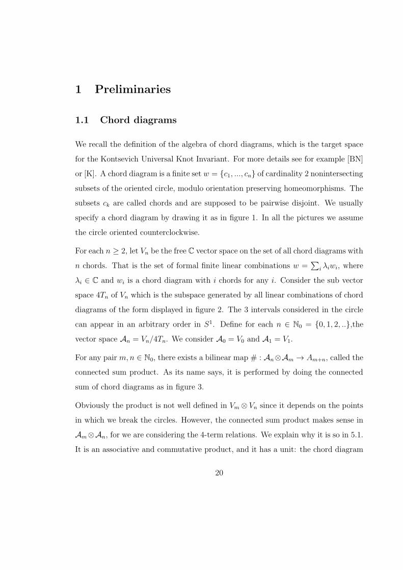
or [K]. A chord diagram is a finite set w = c1, ..., cn of cardinality 2 nonintersecting
subsets of the oriented circle, modulo orientation preserving homeomorphisms. The
subsets ck are called chords and are supposed to be pairwise disjoint. We usually
specify a chord diagram by drawing it as in figure 1. In all the pictures we assume
the circle oriented counterclockwise.
For each n ≥ 2, let Vn be the free C vector space on the set of all chord diagrams with
n chords. That is the set of formal finite linear combinations w =∑
i λiwi, where
λi ∈ C and wi is a chord diagram with i chords for any i. Consider the sub vector
space 4Tn of Vn which is the subspace generated by all linear combinations of chord
diagrams of the form displayed in figure 2. The 3 intervals considered in the circle
can appear in an arbitrary order in S1. Define for each n ∈ N0 = 0, 1, 2, ..,thevector space An = Vn/4Tn. We consider A0 = V0 and A1 = V1.
For any pair m,n ∈ N0, there exists a bilinear map # : An⊗Am → Am+n, called the
connected sum product. As its name says, it is performed by doing the connected
sum of chord diagrams as in figure 3.
Obviously the product is not well defined in Vm⊗ Vn since it depends on the points
in which we break the circles. However, the connected sum product makes sense in
Am⊗An, for we are considering the 4-term relations. We explain why it is so in 5.1.
It is an associative and commutative product, and it has a unit: the chord diagram
20
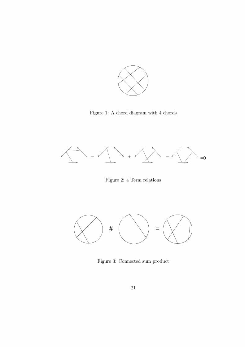
Figure 1: A chord diagram with 4 chords
− + − =0
Figure 2: 4 Term relations
# =
Figure 3: Connected sum product
21
∆( )= +
+ +
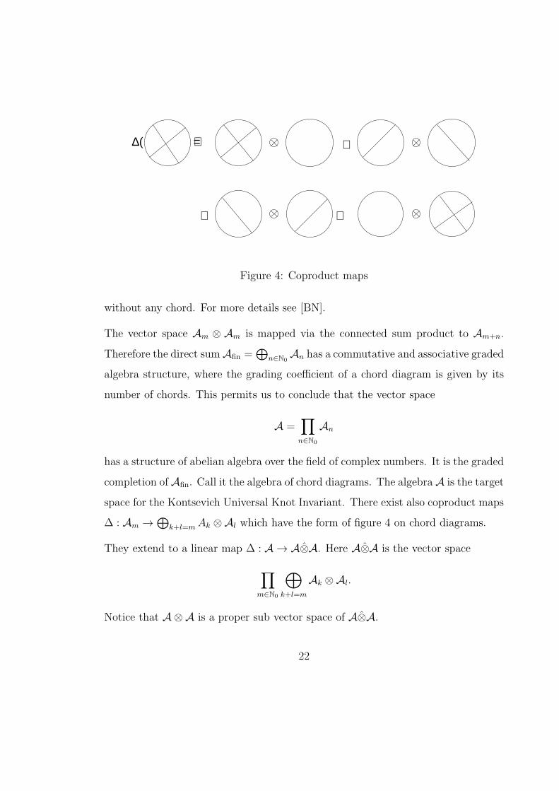
Figure 4: Coproduct maps
without any chord. For more details see [BN].
The vector space Am ⊗ Am is mapped via the connected sum product to Am+n.
Therefore the direct sumAfin =⊕
n∈N0An has a commutative and associative graded
algebra structure, where the grading coefficient of a chord diagram is given by its
number of chords. This permits us to conclude that the vector space
A =∏
n∈N0
An
has a structure of abelian algebra over the field of complex numbers. It is the graded
completion of Afin. Call it the algebra of chord diagrams. The algebra A is the target
space for the Kontsevich Universal Knot Invariant. There exist also coproduct maps
∆ : Am →⊕
k+l=mAk ⊗Al which have the form of figure 4 on chord diagrams.
They extend to a linear map ∆ : A → A⊗A. Here A⊗A is the vector space
∏
m∈N0
⊕
k+l=m
Ak ⊗Al.
Notice that A⊗A is a proper sub vector space of A⊗A.
22
An element w ∈ A is called group like if ∆(w) = w⊗w. That is, if writing w =∑
n∈N0wn with n ∈ An, ∀n ∈ N0 we have
∆(wn) =∑
l+k=n
wk ⊗ wl.
For example, exp(⊖) is a group like element. Here ⊖ is the unique chord diagram
with only one chord. This is a trivial consequence of the fact ∆(⊖) = ⊖⊗1+1⊗⊖.
We have put 1 for the chord diagram without chords.
1.2 The Kontsevich Universal Knot Invariant
We skip for a moment the definition of the (framed) Kontsevich Universal Knot
invariant Z, for which we refer for example to [K], [LM1], [Wi1] and 6.1. For the
unframed version see [CD] and [BN], the classical reference. The sources [LM2] and
[Wi1] unify the two theories in a nice way, as we describe in 6.1.3. We take the
normalisation of the Kontsevich Universal Knot Invariant for which the value of the
unknot is the wheels element Ω of [LNT]. That is Z(O) = Z(∞), cf [BN] pp 447,
or 6.1. This is a different normalisation of the one used in [BN]. We now gather the
properties of the Kontsevich Universal Knot Invariant which we are going to use in
the sequel. Notice that the product we consider in A, the algebra of chord diagrams,
is the connected sum product #.
Theorem 1 There exists a (oriented and framed) knot invariant K 7→ Z(K), where
Z(K) is in the algebra A of chord diagrams. Given a framed knot K, Z(K) satisfies:
1. Z(K) is grouplike, cf [BN]
23

2. If Kf is obtained from K by changing its framing by a factor of 1 then Z(Kf ) =
Z(K) exp(−⊖), cf [LM1].
3. If K∗ is the mirror image of K, and writing Z(K) =∑
n∈N0wn with ωn ∈
An, ∀n ∈ N0 we have Z(K∗) =∑
n∈N0(−1)nwn, cf [CD].
4. If K− is the knot obtained from K by reversing the orientation of it then
Z(K−) =∑
n∈N0S(wn). Here S : An → An is the map that reverses the
orientation of each chord diagram, cf [CD].
5. Z(K#L) = Z(K)Z(L)Z(O)−1, where K#L denotes the connected sum of the
knots K and L and O is the unknot.
Suppose we are given a family of linear maps (weights) Wn : An → C, n ∈ N0. A
knot invariant whose value on each knot is a formal power series with coefficients in
C is called canonical if it has the form
K 7→∑
n∈N0
Wn(wn)hn.
As usual we write Z(K) =∑
n∈N0wn with wn ∈ An, ∀n ∈ N0.
1.3 Infinitesimal R-matrices
Let g be a Lie algebra and U(g) its universal enveloping algebra. Notice U(g) is
generated as an algebra by 1 and g. It has a unique Hopf algebra structure for
which:
1. ∆(X) = X ⊗ 1 + 1⊗X, ∀X ∈ g
24
2. ε(X) = 0, ∀X ∈ g
3. S(X) = −X, ∀X ∈ g
Let g be a Lie algebra over the field C1. An infinitesimal R-matrix of g is a symmetric
tensor t ∈ g ⊗ g such that [∆(X), t] = 0, ∀X ∈ g. The commutator is taken in
U(g)⊗ U(g).
Suppose we are given an infinitesimal R-matrix t. Write t =∑
i ai ⊗ bi. We have∑
j[∆(aj), t]⊗ bj = 0, thus:
∑
i,j
ajai ⊗ bi ⊗ bj − aiaj ⊗ bi ⊗ bj + ai ⊗ ajbi ⊗ bj − ai ⊗ biaj ⊗ bj = 0, (1)
which resembles the 4T relations considered previously. Given a chord diagram w
and an infinitesimal R-matrix t =∑
i ai⊗bi it is natural thus to construct an element
φt(w) of U(g) in the following fashion: Start in an arbitrary point of the circle and
go around it in the direction of its orientation. Order the chords of w by the order
with which you pass them as in figure 5. Each chord has thus an initial and an end
point. Then go around the circle again and write (from the right to the left) aik or
bik depending on whether you got to the initial or final point of the kth chord. Then
sum over all the ik’s. For example for the chord diagram of figure 5 the element
φt(w) is:∑
i1,i2,i3
bi2bi3bi1ai3ai2ai1 .
1We could obviously consider any field, however it needs to be a subfield of C so that the
evaluation of chord diagrams make sense. Notice the the Kontsevich Universal knot invariant has
values in the algebra of chord diagrams with coefficients in Q
25

1
1
2
2
3
3
Figure 5: Enumerating the Chords of a Chord Diagram
See [K] or [CV] for more details. It is possible to prove (we are going to do it in 5.1)
that φt(w) is well defined as an element of U(g), that is it does not depend on the
starting point in the circle. Moreover:
Theorem 2 Let g be a Lie algebra and t ∈ g⊗ g be an infinitesimal R-matrix. The
linear map φt : Vn → U(g) satisfies the 4T relations, therefore it descends to a linear
map φt : An → U(g). Moreover:
1. The image of φt is contained in C(U(g)), the centre of U(g).
2. The degree of φt(w) in U(g) with respect to the natural filtration of U(g) is not
bigger than twice the number of chords of w.
3. Given w ∈ Am and w′ ∈ An we have φt(w#w′) = φt(w)φt(w
′)
4. Consider the map φt,h : A → C(U(g))[[h]] such that if w =∑
n∈N0wn with
wn ∈ An for each n ∈ N0 we have
φt,h =∑
n∈N0
φt(wn)hn.
Then φt,h is a C-algebra morphism.
26

Usually we put φt instead of φt,h to simplify the notation. This is a well known
result. However I could not find a complete proof of it in the literature. A large
part of this thesis depends on it, therefore we will give a proof of the difficult part
of it in 5.1.
Obviously, depending on the Lie algebra and the infinitesimal R-matrix we choose,
the evaluation of φt will satisfy some additional relations to the 4-term relations.
We will give a description of this for the sl(2,C) case in 5.2, following [CV]. As we
will see in the next section, apart from scaling, there exists only one infinitesimal
R-matrix in sl(2,C), and in general in any simple Lie algebra.
1.3.1 Constructing infinitesimal R-matrices
There exists a standard way to construct infinitesimal R-matrices in a Lie algebra
g. Suppose we are given a g-invariant, non degenerate, symmetric bilinear form
<,> in g. Here g-invariance means that we have < [X, Y ], Z > + < Y, [X,Z] >=
0, ∀X, Y, Z ∈ g. If g is semisimple the Cartan-Killing form verifies the properties
above. Take a basis Xi of g and let X i be the dual basis of g∗ . Then it is easy
to show that for any λ ∈ C the tensor t = λ∑
iXi⊗X i is an infinitesimal R-matrix
of g. We are identifying g∗ with g using the nondegenerate bilinear form <,>.
Suppose g is a semisimple Lie algebra and let t =∑
i ai ⊗ bi be an infinitesimal
R-matrix in g. Let also <,> denote the Cartan-Killing form on g. Then the map
g → g such that X 7→ ∑
i < X, ai > bi is an intertwiner of g with respect to its
adjoint representation. Therefore if g is simple it is a multiple λ of the identity.
This permits us to conclude that t = λXi ⊗X i.
Let us now look at the case when g is semisimple. Then g has a unique decomposition
27
of the form g ∼= g1 ⊕ ... ⊕ gn, where each gi is a simple Lie algebra. The Cartan-
Killing form in each gi will yield an infinitesimal R-matrix ti in each gi. Obviously
each linear combination t = λ1t1 + ... + λntn is an infinitesimal R-matrix for g. An
argument similar to the one before proves that any infinitesimal R-matrix in g needs
to be of this form.
It should be said that in the case in which an infinitesimal R-matrix in a Lie algebra
g comes from a non-degenerate, symmetric and g-invariant bilinear form then our
construction of central elements yields the same result as [BN], cf [CV].
1.3.2 Universal U(g)-knot invariants
Recall that the Kontsevich integral is a sum of the form Z(K) =∑
n∈N0wn with
wn ∈ An, ∀n ∈ N0. Let g be a Lie algebra and t an infinitesimal R-matrix of g. We
can consider the composition φt Z. This will yield a knot invariant with values in
the algebra of formal power series over the centre C(U(g)) of U(g). Therefore:
Theorem 3 Let g be Lie algebra and t an infinitesimal R-matrix in g There exists
a framed knot invariant Zt = (φt Z). It has the form:
Zt = (φt Z) : K 7→+∞∑
n=0
(φt Zn)(K)hn, (2)
where (φt Zn)(K) ∈ C(U(g)), n = 0, 1...
If g is simple then according to the results of 1.3.1 there exists essentially only one
infinitesimal R-matrix t. In this case (φt Z) is called the universal U(g) knot
invariant.
28

If g is complex semisimple and t is the infinitesimal R-matrix coming from the
Cartan-Killing form in g, then (φt Z)(K) defines an analytic function from C to
the completion of U(g), where U(g) is given the topology of convergence in its finite
dimensional representations, cf. [PS]. In other words, for any finite dimensional
representation ρ of g in V , the power series ρ(φt Z)(K) converges to a linear
operator V → V , in fact to a multiple of the identity if V is irreducible. The usual
quantum group knot invariants are obtained by taking the trace of these operators.
We will go back to these issues later in 3.3 for the sl(2,C) case. This thesis aims
mostly to consider the case in which we admit infinite dimensional representations.
1.3.3 C[[h]]-valued knot invariants
Let g be a Lie algebra and t be an infinitesimal R-matrix in g. Suppose are given
a morphism f : C(U(g)) → C. Morphisms f like this are usually called central
characters of g. Composing f with Zt = (φt Z) yields a canonical knot invariant
(see the end of 1.2) f φt Z.
Obviously any map f : C(U(g)) → C will define a knot invariant in the same fashion.
However, if f is a morphism then f φt : A 7→ C[[h]] is also a morphism of algebras
thus the properties 2 and 5 of theorem 1 will translate in the obvious way to f φtZ.
It is not difficult to examine the conditions whereby this kind of knot invariants are
unframed. Let t =∑
i ai ⊗ bi be an infinitesimal R matrix in a Lie algebra. Define
Ct =∑
i aibi = φt(⊖). It is a central element of the universal enveloping algebra of g.
Call it the quadratic central element associated with t. The infinitesimal R-matrix
t can be recovered from Ct by the formula
t =∆(Ct)− 1⊗ Ct − Ct ⊗ 1
2.
29

A morphism f : C(U(g)) → C is said to be t-unframed if f(Ct) = 0. From theorem
1, 2 and theorem 2, 3 it is straightforward to conclude that:
Theorem 4 Let g be a Lie algebra with an infinitesimal R-matrix t. Consider also
a morphism f from the centre of U(g) to C. Then the knot invariant f Zt is
unframed if and only if the morphism f is t-unframed.
Notice the Kontsevich integral of each knot is invertible in A. This is because the
term w0 ∈ A0 is the unit of A. We need this fact to prove the last theorem.
1.3.4 A factorisation theorem
Suppose the Lie algebra g ∼= g1 ⊕ g2 is the direct sum of two Lie algebras. If t1 and
t2 are infinitesimal R-matrices in g1 and g2 then t = t1 + t2 is also an infinitesimal
R-matrix in g. Moreover given a chord diagram w we have the following identity:
cf [BN]
φt(w) = (φt1 ⊗ φt2)∆(w).
It is trivial to conclude this from the definition of ∆. We are obviously considering
the standard isomorphism U(g) ∼= U(g1)⊗U(g2) such that (X, Y ) 7→ X ⊗ 1+1⊗Y
for (X, Y ) ∈ g.
If we are given two algebra morphisms fi : C(U(gi)) → C, i = 1, 2, then f = f1 ⊗ f1
is an algebra morphism C(U(g)) ∼= C(U(gi))⊗ C(U(gi) → C. We can thus consider
the knot invariant f Zt. It expresses in a simple form in terms of fi Zti , i = 1, 2.
In fact:
30

Theorem 5 Given any (oriented and framed) knot K we have:
(f Zt)(K) = (f1 Zt1)(K)× (f2 Zt2)(K),
as formal power series
Proof.
Let K be a knot, write Z(K) =∑
n∈N0wn with wn ∈ An, ∀n ∈ N0. We have:
(f Zt)(K) =∑
n∈N0
(f φt)(wn)hn
=∑
n∈N0
(f1 ⊗ f2) (φt1 ⊗ φt2)(∆(wn))hn
=∑
n∈N0
∑
k+l=n
(f1 ⊗ f2) (φt1 ⊗ φt2)(wk ⊗ wl)hn
=∑
n∈N0
∑
k+l=n
[(f1 φt1)(wk)] [(f2 φt2)(wl)] hk+l
= (f1 Zt1)(K)× (f2 Zt2)(K).
This result and proof appears in [GN]
1.4 The Coloured Jones Polynomial
1.4.1 The algebra Uh(sl(2,C))
The coloured Jones Polynomial is constructed out of the finite dimensional represen-
tations of the h-adic Hopf algebra Uh(sl(2,C)), the quantised universal enveloping
algebra of sl(2,C). We will follow the convention of [H]. The algebra Uh(sl(2,C)) is
31

the complete C[[h]]-algebra topologically generated by H , E and F and relations:
HE = E(H + 2), HF = F (H − 2), (EF − FE) =sinh(hH/2)
sinh(h/2).
Let q = exp(h), v = exp(h/2) and K = exp(hH/2). Set [n] = [n]h = vn−v−n
v−v−1and
[n]h! = [1][2]...[n]. The algebra Uh(sl(2,C)) can be given a structure of ribbon quasi
Hopf algebra with R-matrix
R = v12H⊗H
+∞∑
n=0
vn(n+1)
2
[n]!(v − v−1)nEn ⊗ F n,
and group like element G = K. Therefore, the ribbon element θ is
θ = K−1∑
S
(ti)si,
where R =∑
i si ⊗ ti. See [RT], for example for the definition of ribbon Hopf
algebras.
The theory of finite dimensional representations of Uh(sl(2,C)) is similar to the
representation theory of sl(2,C). A complete set of indecomposable representations
of Uh(sl(2,C)) made out of the representations of spin α ∈ 12N0. These are repre-
sentations in the free C[[h]]-module with basis v0, ..., v2a and actions:
Hvi = (n− 2i)vi, Evi = [n+ 1− i]vi−1, F vi = [i+ 1]vi+1.
Alternatively, we can see it as a representation in Vα
, the free C[[h]] module with
basis vα−α, ..., vαa, considering this actions of generators of Uh(sl(2,C)):
Hvαiα = 2aiv
αiα,
Evαiα = v−
12 viα
√
[α + iα + 1][α− iα]vαiα+1,
F vαiα = v+
12 v−iα
√
[α− iα + 1][α + iα]vαiα−1.
32

The possibility of writing the representations in this way will be important later.
Notice that the terms under the square roots always define holomorphic functions in
a neighbourhood of zero, thus elements of C[[h]]. These are all the indecomposable
finite dimensional representations of Uh(sl(2,C)). See [KS] or [CP].
1.4.2 Ribbon Hopf Algebras, knot invariants and the Coloured Jones
Polynomial
Recall that any finite dimensional representation V of a ribbon Hopf algebra Aalways define a framed knot invariant I. Let us say what our conventions are. See
[K],[RT] or [CP] for more details. Let R =∑
i si ⊗ ti be the R-matrix of A and
θ its ribbon element. Recall the group like element G of A is G = uθ−1 where
u =∑
i S(ti)si
Let A be a ribbon Hopf algebra with an R-matrix R =∑
i si ⊗ ti, and group like
element G. Let V be a finite dimensional representation of A. Choose a basis viof V and let vi be its dual basis of V ∗. Notice V ∗ is also a representation of Aunder the rule af(v) = f(S(a)v), v ∈ V, f ∈ V ∗, a ∈ A . If K is a framed knot then
I(K) is calculated from a regular projection of K under the rules:
F(→∪ ) = 1 7→∑
i
vi ⊗ vi,
F(←∪ ) = 1 7→∑
i
vi ⊗G−1vi,
F(→∩ ) = f ⊗ v 7→ f(v),
F(←∩ ) = v ⊗ f 7→ f(Gv),
F(X+) = v ⊗ w 7→∑
i
tiw ⊗ siv,
33

Figure 6: Knot Generators →∪ ,←∪ ,→∩ ,←∩ , X+ and X−
Figure 7: 1-framed unknot
F(X−) = w ⊗ v 7→∑
i
siw ⊗ tiv,
where R =∑
i si ⊗ ti and R−1 =
∑
i si ⊗ ti
For example the evaluation for the 1-framed unknot in figure 7 is:
1 7→∑
i
vi ⊗G−1vi 7→∑
i,j
tjG−1vi ⊗ sjv
i 7→∑
i,j
sjvi(GtjG
−1vi) =
∑
i,j
vi(S(sj)GtjG−1vi) = trv 7→
∑
j
vi(S(sj)GtjG−1v = trv 7→ θu−1v
= trv 7→ θG−1v.
Definition 6 The coloured Jones polynomial Jα, where α ∈ 12N0 is, by definition
the framed knot invariant made out of the the ribbon Hopf algebra Uh(sl(2,C)) and
the representation of spin α of it
Therefore the coloured Jones polynomial is a knot invariant with values in C[[h]].
In fact if we look at 1.4.1 it is trivial to conclude that Jα(K) is always a Laurent
34

polynomial in exp(h/4) = v12 .
1.4.3 The coloured Jones polynomial and central characters
Let g be a simple Lie algebra and ρ a representation of g in the vector space V .
Then ρ is said to admit a central character if every element of C(U(g)) acts on
V as a multiple of the identity. In this case there exists an algebra morphism
λρ : C(U(g)) → C such that ρ(a)(v) = λρ(a)v, ∀a ∈ C(U(g)), v ∈ V . The algebra
morphism λρ is called the central character of the representation ρ. In particular, if
g is a Lie algebra with an infinitesimal R-matrix t then given any representation ρ
of g with a central character, we can construct the knot invariant (λρ φt Z), as
in 1.3.3. It has values in the algebra C[[h]] of formal power series over C.
Recall that the coloured Jones polynomial Jα, where α ∈ 12N0 is, by definition the
framed knot invariant made out of the the ribbon Hopf algebra Uh(sl(2,C)) and the
representation of spin α of it. It is therefore a framed knot invariant with values
in C[[h]]. However, apart from normalisation, the coloured Jones polynomial is
a particular example of this construction. Let t be the infinitesimal R-matrix of
sl(2,C) corresponding to the bilinear form in it which is minus the Cartan-Killing
form. Notice a nice form for t:
t = −1
4(σX ⊗ σX + σY ⊗ σY + σZ ⊗ σZ),
where σX , σY , σZ are the Pauli Matrices. See 2.1. Another expression for t appears
in 1.4.6. Consider for any α ∈ 12N0 the representation ρ
αof sl(2,C) with spin α, thus
ραadmits a central character which we denote by λα. Given a framed knot K Let
Jα(K) denote the framed Coloured Jones Function of it. Notice we ”colour” the
35

Jones polynomial with the spin of the representation, rather than with the dimension
of it. The last one is the usual convention.
Theorem 7 We have:
Jα(K)
2α + 1= (λα Zt)(K), ∀α ∈ 1
2N0. (3)
This is well known, though non trivial. A path for proving it relies upon the frame-
work of quasi Hopf algebras and the notion of gauge transformations on them. This
is described by Drinfeld in [D1] and [D2]. The context in which we need to apply
it is the quantised universal enveloping algebras one. In this case some rigidity re-
sults ensure the above theorem is true. All this is described in detail in the same
references. For a complete discussion, see [LM1] or[K].
1.4.4 Melvin-Morton Theorem and z-Coloured Jones Polynomial
Let K be a framed knot write
Jα(K)
2α+ 1=∑
n∈N0
Jαn (K)hn.
It is a well known result that given a knot K then Jan(K) is a polynomial in α with
degree at most 2n, cf [MM], [C]. This is known as Melvin-Morton theorem. The
fact it is a polynomial is consequence of the fact that the centre of U(sl(2,C)) is
generated by the Casimir element of it, together with part 1 of Theorem 2. Notice
the Casimir element act as α(α + 1)/2 in the representation of spin α. The fact it
is of degree 2n is clear from our discussion in 1.4.6. Alternatively we can prove it
36
from part 2 of theorem 2 2. We will go back to this in 3.3. Therefore we can write:
Jα(K)
2α+ 1=∑
n∈N0
2n∑
k=0
Jn,k(K)αkhn, (4)
where the constants Jn,k(K) are uniquely determined, therefore defining a framed
knot invariant. For any complex number z it thus makes sense to consider the
z-coloured Jones polynomial:
Jz(K)
2z + 1=∑
n∈N0
Jzn(K)(z)hn.
This yields thus a knot invariant whose value in a knot is a formal power series in
two variables:
K 7→∑
m,n∈N0
Jn,k(K)zkhn.
with Jn,k(K) = 0 for k > 2n. A major part of this thesis aims to investigate
whether or not this kind of series defines an analytic function in two variables. As
we mentioned in the introduction, and are going to prove in 4.1, they can have a
zero radius of convergence, thus this can only be made precise in a perturbation
theory point of view, as we will see in 4.2. This relates to the question of whether
it is possible to define numerical knot invariants out of the infinite dimensional
representations of SL(2,R), see theorem 26, and of the Lorentz Group after Theorem
16. It is known that if α is a half integer then
Jα(K)
2α + 1=∑
m∈N0
(
2n∑
k=0
Jn,k(K)αk
)
hn
2The part of the centre of U(sl(2,C)) of degree smaller than 2n is generated by polynomials in
the Casimir element of sl(2,C) having degree n, see [VAR] for example
37

defines an analytic function in h. See the comments at the end of 1.3.2 and 3.3.
1.4.5 First example: The Unknot
For the unknot O the series Jz(O)/(2z + 1) has a non zero radius of convergence
at any point z ∈ C. The proof is not very difficult for we can have an explicit
expression for it. Define, for each z ∈ C the meromorphic function:
Fz(h) =1
2z + 1
sinh((2z + 1)h/2)
sinh(h/2).
Thus for each α ∈ 12N0 we have
Fα(h) =Jα(O)
2α + 1=∑
n∈N0
Jαn (O)hn.
Consider the expansion:
Fz(h) =∑
n∈N0
c(z)nhn.
It is not difficult to conclude that each c(z)n is a polynomial in z for fixed n.
Moreover c(α)n = Jαn (O), ∀α ∈ 12N0. This implies
Jz(O)
2z + 1= Fz(h),
as power series in h. In particular the power series for the unknot are convergent.
This means it makes sense to speak about the quantum dimension of the represen-
tations of spin z, which are going to be defined later. To be more precise we made
sense of the quantum dimension of them divided by their dimension as vector spaces.
38

But notice the dimension of a representation of spin z with z /∈ 12N0 is infinite. For
some more explicit examples see 3.3.
1.4.6 A representation interpretation of the z-Coloured
Jones Polynomial
We can give an interpretation of the z-coloured Jones polynomial in the framework
of central characters. To this end, define the following elements of sl(2,C):
H =
1 0
0 −1
, E =
0 1
0 0
, H =
0 0
1 0
.
Then the infinitesimal R-matrix which we are considering in sl(2,C) expresses in
the form:
t = −1
4
(
E ⊗ F + F ⊗E +H ⊗H
2
)
.
Notice that t is defined out of the inner product in sl(2,C) which is minus the
Cartan-Killing form. In particular, the Casimir element C of sl(2,C) is equal to
−Ct, where Ct is the quadratic central element associated with t. Recall subsection
1.3. The exact value of the Casimir element of U(sl(2,C)) in this basis is:
C =1
4
(
EF + FE +H2
2
)
Given a half integer α, the representation space Vα
of the representation of spin α has
a basis of the form v0, ..., v2α. The action of the elements E, F and H of sl(2,C)
in Vα
is:
Hvk = (k − α)vk,
39

Evk = (2α− k)vk+1,
F vk = kvk−1.
For a complex number z /∈ 12N0, it makes sense also to speak about the representation
ρzof spin z. Consider V
z
as being the infinite dimensional vector space which has the
basis v2z, v2z−1, v2z−2, .... Then the representation ρzof spin z is defined in the
form:
Hvk = (k − z)vk; k = 2z, 2z − 1, ...,
Evk = (2z − k)vk+1; k = 2z, 2z − 1, ...,
F vk = kvk−1; k = 2z, 2z − 1, ....
The representations of spin z /∈ 12N0 have a central character λz, since it is easily
proved that each intertwiner Vz
→ Vz
must be a multiple of the identity. But see
[VAR], 4.10.2. and 3.3, namely they are the unique cyclic highest weight represen-
tations with maximal weight z, this relative to the usual Borel decomposition of
sl(2,C). Consider, given z ∈ C, the framed knot invariant (λz Zt). Where, if α is
half integer, λα is the central character of the usual representation of spin α. See
1.3.3. Given a framed knot K it has the form:
(λz Zt)(K) =∑
n∈N0
Rzn(K)hn,
where, by definition:
Rzn(K) = (λz φt)(wn) =
∑
n∈N0
λz(φt(wn))hn,
40
for
Z(K) =∑
n∈N0
wn, wn ∈ An, ∀n ∈ N0.
AlsoJα(K)
2z + 1=∑
n∈N0
Rαn(K)hn, ∀α ∈ 1
2N
Suppose w is a chord diagram with n chords. Let us have a look at the dependence
of λz(φt(w)) in z. It is not difficult to conclude that it is a polynomial in this
variable of degree at most 2n. This is a trivial consequence of the definition of the
central element φt(w) as well as the kind of action of the terms appearing in the
infinitesimal R-matrix t in Vz
. For more details see 6.2.1 and 3.3. In particular if K
is a framed knot then Rzn(K) is a polynomial in z. Since by theorem 7 we also have
Rαn(K) = Jαn (K), ∀α ∈ 1
2N0, we can conclude:
Jz(K)
2z + 1= (λz Z)(K),
which gives us an equivalent definition of the z-coloured Jones Polynomial.
The central characters of the representations of imaginary spin are actually the
infinitesimal characters, cf [Kir] and 3.1, of the unitary representations of SL(2,R)
in the principal series, cf [L], with the same parameter. See 5.3 for the proof of this.
Notice however that the derived representation of them in sl(2,R)⊗R C ∼= sl(2,C)
is not any of the representation of imaginary spin just defined. We will consider this
point of view later in 3.3.
41

2 The Lorentz Group and knot invariants
Let g be a semisimple Lie Algebra. As proved by Drinfeld in [D1], there is a one to
one correspondence between gauge equivalence classes of quasitriangular quantised
universal enveloping algebras H of g over C[[h]], cf [K], and infinitesimal R-matrices
in g. Let us be more explicit about this. It is implicit in the definition of a quantised
universal enveloping algebra H that there exists a C-algebra morphism f : H/hH →U(g). Having chosen such morphism, the canonical 2-tensor of A is defined as
t = f((R21R − 1)/h). It is an infinitesimal R-matrix of A. See [D1]. Here R
denotes the universal R-matrix of H. In the case of Uh(sl(2,C)) this tensor t is the
infinitesimal R-matrix in sl(2,C) coming from the Cartan Killing form. The same
happens for the Drinfeld-Jimbo quantisation of any semisimple Lie algebra. See [K].
Actually, if H quantises the pair (g, r) where r is a classical r-matrix in g, see [CP],
then t is the symmetrisation of r.
In general, each quantised universal enveloping algebra can be given a structure of
a ribbon quasi Hopf algebra (as defined in [AC] for example), and therefore there is
a knot invariant attached each finite dimensional representation of it, or what is the
same, of g. These knot invariants take their values in the ring of formal power series
over C. If the representation used is finite dimensional and irreducible then it has a
central character. In particular the framework of last section can be applied, using
the infinitesimal R matrix t which is the canonical 2 tensor of H. It is a deep result
that with these choices the two approaches for knot invariants are the same, up to
division by the dimension of the representation considered. This is a generalisation
of theorem 37 to arbitrary semisimple Lie algebras. To be more precise we need also
to change the sign of the infinitesimal R-matrix t, cf [K].
42

In the case in which we consider a q-deformation of the universal enveloping algebra
of a Lie algebra g, then no such classification of gauge equivalence classes of quantised
universal enveloping algebras exists. But sometimes it is possible to make sense
of the formula for t. This is because we have a q-parametrised family of braided
Hopf algebras that tends to the universal enveloping algebra of g as q goes to 1.
Alternatively they can be seen as particularisations of the C[[h]]-algebras Uh(g) to
complex q.
As we mentioned in the introduction, despite the fact that the q-deformed Drinfeld-
Jimbo quantised universal enveloping algebras Uq(g) of semisimple Lie algebras are
not honest ribbon Hopf algebras, their category of finite dimensional representations
is a ribbon category. That is they have formal R-matrices and ribbon elements,
which make sense when acting in their finite dimensional representations. We will
see this in chapter 7. The target space for the knot invariants in this context is
the complex plane. These numerical knot invariants can be obtained, apart from
rescaling, by summing the powers series which appear in context of h-adic Drinfeld-
Jimbo algebras; in other words by summing the power series that come out of the
approach making use the Kontsevich Integral and using the infinitesimal R-matrix
which is the heuristic canonical 2-tensor t of Uq(g).
Let us pass now to the quantum Lorentz Group D = Uq(sl(2,C)R) as defined in
[BR1] and [BR2]. It is a quantum group depending on a parameter q ∈ (0, 1).
We will make a complete study of it in chapter 7. As said in the introduction, we
wish to analyse the question of whether or not there exists a knot theory attached
to the infinite dimensional representations of the Quantum Lorentz Group. The
situation is more or less the same of the case of q-Drinfeld-Jimbo algebras. Namely
we have a formal R-matrix which comes from its structure of a quantum double
43

as well as a formal ribbon element. It is possible to describe how they act in
the unitary representations of D. The situation is simpler if the minimal spin of
the representation is equal to zero, in which case the representation is said to be
balanced. Representations of this kind are called simple in [NR]. In this context,
the ribbon element acts as the identity and therefore the knot invariants obtained
are unframed. Since we have a formal R-matrix and a formal ribbon element, given
a knot diagram it is thus possible to make a formal Reshetikhin-Turaev evaluation
of a knot invariant. This will yield an infinite sum for any of those. We will give a
description of this construction in Chapter 7.
One natural thing to do would be analysing whether the ”derivatives” of these
sums in zero define or not Vassiliev invariants, or whether is possible to make sense
of them, in the framework of Kontsevich Universal Invariant. It is not difficult
to find an expression for an heuristic canonical 2-tensor of the quantum Lorentz
group. Also the unitary representations of the Quantum Lorentz Group in the
principal and complementary series have a classical counterpart. They are infinite
dimensional representations of the Lie algebra of the Lorentz group which admit a
central character, and therefore the framework of the last section can be used. This
is the program we wish to consider now. We will prove that the knot invariants that
we obtain are the ones defined out the infinite dimensional representations of the
Quantum Lorentz Group3 later in Chapter 7.
3Or more precisely the asymptotic expansion of these
44

2.1 The Lorentz Algebra
Consider the complex Lie group SL(2,C). Its Lie algebra sl(2,C) is a complex Lie
algebra of dimension 3. A basis of sl(2,C) is σX , σY , σZ where
σZ =1
2
i 0
0 −i
, σX =1
2
0 i
i 0
, σY =1
2
0 −1
1 0
.
The commutation relations are:
[σX , σY ] = σZ , [σY , σZ ] = σX , [σZ , σX ] = σY .
We can also consider a different basis H+, H−, H3, where
H+ = iσX − sY , H− = iσX + iσY , H3 = iσZ .
The new commutation relations being:
[H+, H3] = −H3, [H−, H3] = H−, [H+, H−] = 2H3.
Restricting the ground field with which we are working to R, we obtain the 6 di-
mensional real Lie algebra sl(2,C)R, the realification of sl(2,C).
Definition 8 The Lorentz Lie algebra L is defined as being the complex Lie algebra
which is the complexification of sl(2,C)R. In other words L = sl(2,C)R ⊗R C. It is
therefore a complex Lie algebra of dimension 6. The Lorentz algebra is the complex
algebra U(L) which is the universal enveloping algebra of the complex Lie algebra L.
The set σX , BX = −iσX , σY , BY = −iσY , σZ , BZ = −iσZ is a real basis of
45
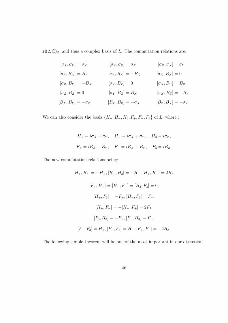
sl(2,C)R, and thus a complex basis of L. The commutation relations are:
[σX , σY ] = σZ [σY , σZ ] = σX [σZ , σX ] = σY
[σZ , BX ] = BY [σY , BX ] = −BZ [σX , BX ] = 0
[σZ , BY ] = −BX [σY , BY ] = 0 [σX , BY ] = BZ
[σZ , BZ ] = 0 [σY , BZ ] = BX [σX , BZ ] = −BY
[BX , BY ] = −σZ [BY , BZ ] = −σX [BZ , BX ] = −σY .
We can also consider the basis H+, H−, H3, F+, F−, F3 of L, where :
H+ = iσX − σY , H− = iσX + σY , H3 = iσZ ,
F+ = iBX − BY , F− = iBX +BY , F3 = iBZ .
The new commutation relations being:
[H+, H3] = −H+, [H−, H3] = −H−, [H+, H−] = 2H3,
[F+, H+] = [H−, F−] = [H3, F3] = 0,
[H+, F3] = −F+, [H−, F3] = F−,
[H+, F−] = −[H−, F+] = 2F3,
[F3, H3] = −F+, [F−, H3] = F−,
[F+, F3] = H+, [F−, F3] = H−, [F+, F−] = −2H3.
The following simple theorem will be one of the most important in our discussion.
46

Theorem 9 There exists one (only) isomorphism of complex Lie algebras τ : sl(2,C)⊕sl(2,C) → L ∼= sl(2,C)R ⊗R C such that:
σX ⊕ 0 7→ σX − iσX ⊗ i
2=σX + iBX
2,
0⊕ σX 7→ σX + iσX ⊗ i
2=σX − iBX
2,
σY ⊕ 0 7→ σY − iσY ⊗ i
2=σY + iBY
2,
0⊕ σY 7→ σY + iσY ⊗ i
2=σY − iBY
2,
σZ ⊕ 0 7→ σZ − iσZ ⊗ i
2=σZ + iBZ
2,
0⊕ σZ 7→ σZ + iσZ ⊗ i
2=σZ − iBZ
2.
And thus we have also a Hopf algebra isomorphism
τ : U(sl(2,C))⊗ U(sl(2,C)) → U(L).
Proof. Easy calculations
Given X ∈ sl(2,C), define X l = τ(X ⊕ 0), Xr = τ(0 ⊕ X). And analogously for
X ∈ U(sl(2,C)). We have:
H l+ =
H+ + iF+
2, H l
− =H− + iF−
2, H l
+ =H3 + iF3
2,
Hr+ =
H+ − iF+
2, Hr
− =H− − iF−
2, Hr
+ =H3 − iF3
2.
Consider also C l = τ(C ⊗ 1) and Cr = τ(1⊗C), where C is the Casimir element of
sl(2,C) defined in 1.4.6. The elements C l and Cr are called Left and Right Casimirs
47

and their explicit expression is:
4C l =H2
3 − F 23
2+ i
H3F3
2+ i
F3H3
2
+H+H−
4+ i
H+F−4
+ iF+H−
4− F+F−
4
+H−H+
4+ i
H−F+
4+ i
F−H+
4− F−F+
4,
and
4Cr =H2
3 − F 23
2− i
H3F3
2− i
F3H3
2
+H+H−
4− i
H+F−4
− iF+H−
4− F+F−
4
+H−H+
4− i
H−F+
4− i
F−H+
4− F−F+
4.
We can also consider the left and right image under τ ⊗ τ of the infinitesimal R-
matrix of U(sl(2,C)). We take now t ∈ sl(2,C)⊗ sl(2,C) as being the infinitesimal
R-matrix coming from the Cartan-Killing form. That is minus the one considered
in 37. These left and right infinitesimal R-matrices are:
4tl =H3 ⊗H3
2− F3 ⊗ F3
2+ i
H3 ⊗ F3
2+ i
F3 ⊗H3
2
+H+ ⊗H−
4+ i
H+ ⊗ F−4
+ iF+ ⊗H−
4− F+ ⊗ F−
4
+H− ⊗H+
4+ i
H− ⊗ F+
4+ i
F− ⊗H+
4− F− ⊗ F+
4,
and
48

4tr =H3 ⊗H3
2− F3 ⊗ F3
2− i
H3 ⊗ F3
2− i
F3 ⊗H3
2
+H+ ⊗H−
4− i
H+ ⊗ F−4
− iF+ ⊗H−
4− F+ ⊗ F−
4
+H− ⊗H+
4− i
H− ⊗ F+
4− i
F− ⊗H+
4− F− ⊗ F+
4.
Any linear combination atl + btr of the left and right infinitesimal R-matrices is an
infinitesimal R-matrix for L. In fact all them are of this form as proved in 1.3.1.
We wish to consider the combination tL = tl − tr. That is
tL = i1
4H3 ⊗ F3 +
1
4iF3 ⊗H3 +
i
8H− ⊗ F+ +
i
8F− ⊗H+ +
i
8H+ ⊗ F− +
i
8F+ ⊗H−.
Notice another expression of it:
tL =i
8(BX ⊗ σX + σX ⊗BX +BY ⊗ σY + σY ⊗ BY +BZ ⊗ σZ + σZ ⊗ BZ) .
The quadratic central element of U(L) associated with tL is:
CL = CtL = iH3F3
4+ i
F3H3
4+ i
H+F−8
+ iF+H−
8+ i
H−F+
8+ i
F−H+
8
The reason why we consider this particular combination of the left and right infinites-
imal R-matrices is because it corresponds to the heuristic canonical two tensor of
the Quantum Lorentz group Uq(sl(2,C)R) considered in [BR2]. Notice it is the sym-
metrisation of the classical r-matrix of sl(2,C)R, see [BNR] page 19. The knot theory
obtained from tL and the unitary representations of the Lorentz Group ought to be
related to any knot invariants that can be defined from the unitary representations
49

of Uq(sl(2,C)R) for q ∈ (0, 1). We shall see in the last chapter (Theorem 136) that
this is the case, at least for balanced representations.
The general case in which we admit other infinitesimal R-matrices is not more diffi-
cult, however the relations with the knot theory coming from the Quantum Lorentz
Group is not as transparent. This is because we are changing the quantum group
with which we are working. See the introduction to this chapter. Another interesting
combination of the Left and Right infinitesimal R-matrices is the following:
tL = tl+tr =1
8(σX⊗σX−BX⊗BX+σY ⊗σY −BY ⊗BY +σZ⊗σZ−BZ⊗BZ). (5)
It corresponds to working with Uq(su(2))⊗ Uq(su(2)), with q in the unit circle.
Both tL and tL are identified with the obvious invariant non-degenerate bilinear
forms in the Lie algebra of the Lorentz group 4. In fact, it is possible to prove that
the Chern-Simons functional
CS(A) = exp
(
i1
4π
∫
M
tr
(
A ∧ dA+2
3A ∧ A ∧ A
))
(6)
is gauge invariant if and only if tr is defined out of the non-degenerate, invariant,
bilinear form in L associated with ntL + stL, with n ∈ Z and s ∈ C, see [W]. Here
A denotes an L-valued 1-form in a 3 manifold M .
4The first is the imaginary part of the Cartan Killing form in sl(2,C) whereas the second is the
real part of it
50

2.1.1 The irreducible Balanced Representations of the Lorentz Group
Let us be given a complex number p = |p|eiθ, 0 ≤ θ < 2π different from zero. We
define once for all5 the square root√p of p as being
√
|p|eiθ =√
|p|ei θ2 . For m ∈ Z
define the set Wm = p ∈ C : |p| /∈ N|m|+1, where, in general, Nm = m,m+1, ...,for any m ∈ N. Consider the set P = (m, p) : m ∈ Z, p ∈ Wm. Define, for any
α ∈ N and (p,m) ∈ P:
Cα(p,m) =i
α
√
(α2 − p2)(α2 −m2)
4α2 − 1,
Bα(p,m) =ipm
α(α + 1).
Thus Cα(p,m) 6= 0, α = |m|+ 1, |m|+ 2..., ∀p ∈ Wm
Consider the complex vector space
V (m) =⊕
α∈N|m|
Vα
,
where Vα
denotes the representation space of the representation of sl(2,C) of spin
α. The set vαi, i = −α,−α + 1, ..., α;α ∈ N|m| is a basis of V (m). Consider the
inner product in V (m) that has the basis above as an orthonormal basis. Define
also V (m) as being the Hilbert space which is the completion of V (m).
Given (p,m) ∈ P, consider the following linear operators acting on V (m):
H3vαk = kv
αk, k = −α,−α + 1, ..., α, α ∈ N|m|,
H−vαk =
√
(α + k)(α− k + 1)vαk−1, k = −α,−α + 1, ..., α
5We will see in a second that this choice is totally irrelevant
51

H+vαk =
√
(α + k + 1)(α− k)vαk+1, k = −α,−α + 1, ..., α,
F+vαk = Cα(m, p)
√
(α− k)(α− k − 1) vα−1
k+1
−Bα(m, p)√
(α + k + 1)(α− k)vαk+1
+ Cα+1(m, p)√
(α + k + 1)(α + k + 2) vα+1
k+1,
k = −α,−α + 1, ..., α, α ∈ N|m|,
F−vαk = −Cα(m, p)
√
(α + k)(α + k − 1) vα−1
k−1
−Bα(m, p)√
(α− k + 1)(α+ k)vαk+1
− Cα+1(m, p)√
(α + 1)2 − k2 vα+1
k,
k = −α,−α + 1, ..., α, α ∈ N|m|,
F3vαk = Cα(m, p)
√α2 − k2 v
α−1k − Bα(m, p)kv
αk
− Cα+1(m, p)√
(α + 1)2 − k2 vα+1
k,
k = −α,−α + 1, ..., α, α ∈ N|m|.
Obviously we are considering vαk = 0 if k > α or k < −α. We have the following
theorem, whose proof can be found in [GMS]
Theorem 10 If (p,m) ∈ P, the operators H−, H+, H3, F−, F+, F3 define an infinite
dimensional representation of the Lorentz algebra.
Notice that the representations (m, p) and (−m,−p) are equivalent. This has a
trivial proof.
52

In fact, the operators displayed before define a representation of the Lorentz algebra
if and only if:
(Bα(α + 1)− (α− 1)Bα−1)Cα = 0,
(Bα+1(α + 2)− αBα)Cα+1 = 0,
(2α− 1)C2α − (2α + 3)C2
α+1 − B2α = 1.
(7)
The quantum case will be very similar. We have put Ba(m, p) = Bα and Cα(m, p) =
Cα to simplify. See [GMS]. In particular the square root we choose in the definition
of Cα(m, p) is not important if we want to define a representation. In addition,
making the transformation vαi 7→ (−1)cαv
αi where cα ∈ 0, 1 tells us the choice of
the square root does not affect the representation apart from isomorphism, therefore
being totally irrelevant.
Denote the representations above by ρ(m, p) : (m, p) ∈ P. One can prove with
no difficulty that they have a central character, for any intertwiner V (m) → V (m)
needs to send each space Vα
to itself and act on it has a multiple of the identity.
Considering the action of F+, for example, we conclude that the multiples are the
same in each space Vα
. See [BR2], proof of irreducibility in theorem 3. Therefore
Theorem 11 For any (m, p) ∈ P the representation ρ(m, p) of L admits a central
character λm,p.
For any (m, p) ∈ P the representation ρ(m, p) of L can always be integrated to a
representation R(m, p) of the Lorentz group in the completion V (m) of V (m), or
to be more precise of its connected component of the identity, see [GMS] II.4.7.
The resulting representation is unitary if and only if p is purely imaginary, for
any m ∈ N0, in which case the representation is said to belong to the principal
series, or if m = 0 and p ∈ [0, 1) in which case the representation is said to belong
53
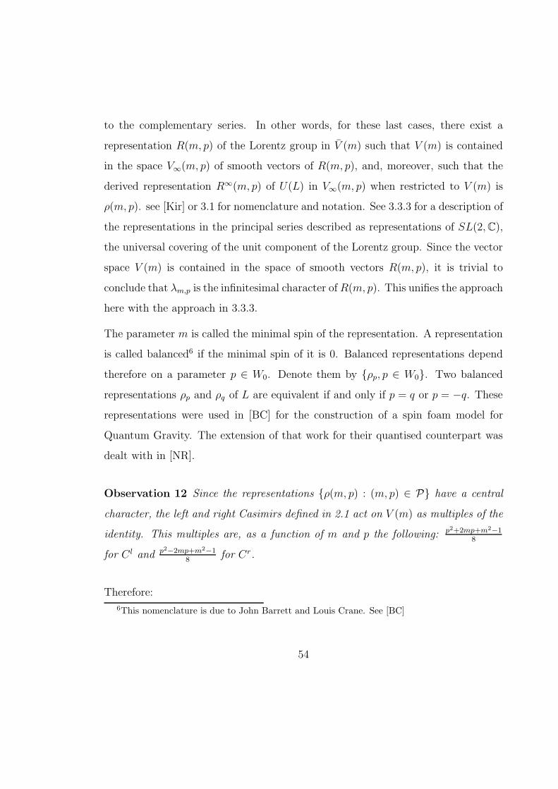
to the complementary series. In other words, for these last cases, there exist a
representation R(m, p) of the Lorentz group in V (m) such that V (m) is contained
in the space V∞(m, p) of smooth vectors of R(m, p), and, moreover, such that the
derived representation R∞(m, p) of U(L) in V∞(m, p) when restricted to V (m) is
ρ(m, p). see [Kir] or 3.1 for nomenclature and notation. See 3.3.3 for a description of
the representations in the principal series described as representations of SL(2,C),
the universal covering of the unit component of the Lorentz group. Since the vector
space V (m) is contained in the space of smooth vectors R(m, p), it is trivial to
conclude that λm,p is the infinitesimal character ofR(m, p). This unifies the approach
here with the approach in 3.3.3.
The parameter m is called the minimal spin of the representation. A representation
is called balanced6 if the minimal spin of it is 0. Balanced representations depend
therefore on a parameter p ∈ W0. Denote them by ρp, p ∈ W0. Two balanced
representations ρp and ρq of L are equivalent if and only if p = q or p = −q. Theserepresentations were used in [BC] for the construction of a spin foam model for
Quantum Gravity. The extension of that work for their quantised counterpart was
dealt with in [NR].
Observation 12 Since the representations ρ(m, p) : (m, p) ∈ P have a central
character, the left and right Casimirs defined in 2.1 act on V (m) as multiples of the
identity. This multiples are, as a function of m and p the following: p2+2mp+m2−18
for C l and p2−2mp+m2−18
for Cr.
Therefore:
6This nomenclature is due to John Barrett and Louis Crane. See [BC]
54

Proposition 13 If the infinitesimal R-matrix on U(L) is the tensor tL defined in
2.1 then the central characters of the balanced representations λp, p ∈ W0 are
tL-unframed. Recall the nomenclature introduced before theorem 4.
This can obviously be proved without using the explicit expression of the action of
the Casimir elements.
Notice also that we can consider the minimal spin of the representations considered
to be also to be an half integer, making the obvious change in the form of the repre-
sentation. These kind of representations cannot be integrated to representations of
the Lorentz group, even though they define representations of SL(2,C). They are
called two-valued representations of the Lorentz group in [GMS] .
2.2 The Lorentz Knot Invariant
Consider again the infinitesimal R-matrix tL = tl−tr of the Lorentz Lie algebra. We
consider for each (m, p) ∈ P the representation ρ(m, p) of L. It has a central charac-
ter λm,p. We propose to consider the framed knot invariants X(m, p) : (m, p) ∈ P,such that for any knot:
K 7→ X(m, p,K) = (λm,p Ztl)(K) = (λm,p φtL Z)(K).
Recall the notation of 1.3. Notice X(m, p) = X(−m,−p) for the representations
ρm,p and ρ−m,−p are equivalent.
The value of X(m, p) in a framed knot K is therefore a formal power series with
coefficients in C. It is a difficult task to analyse the analytic properties of such
power series. We expect they will be perturbation series for some numerical knot
55

invariants that can be defined. This is the main subject of chapter 4.
As we have seen, if m = 0, that is in the case of balanced representations, the
central character λp is tL-unframed. This is also the case for p = 0. Notice we have
an explicit expression for the action of the left and right Casimir elements of L.
Therefore
Theorem 14 The knot invariant X(m, p) with (m, p) ∈ P is unframed if and only
if m = 0 or p = 0.
Obviously, for different combinations of the left and right infinitesimal R-matrices,
the representations which have unframed central characters with respect to it are
different. This gives us a way to define an unframed knot invariant out of any
(m, p) ∈ P. But notice this can be done without changing the infinitesimal R-
matrix tL of L, since we know how the invariants behave with respect to framing,
cf theorem 1.
2.2.1 Finite Dimensional Representations
Let us now analyse the knot invariants that come out of the finite dimensional
representations of the Lorentz group. We are mainly interested in the representations
which are irreducible.
Since we have the isomorphism U(L) ∼= U(sl(2,C))⊗ U(sl(2,C)), the finite dimen-
sional irreducible representation of U(L), or what is the same of L, are classified by a
pair (α, β) of half integers. That is each finite dimensional irreducible representation
of L is of the form ρα ⊗ ρ
βas a representation of U(L) ∼= U(sl(2,C)) ⊗ U(sl(2,C)).
There is an alternative way to construct these finite dimensional representations
56

that shows their close relation with the infinite dimensional representations, [GMS].
Let us explain how the process goes. It is very similar to the sl(2,C) case.
Considerm = α−β and p = α+β+1. Notice that now Cα(m, p) 6= 0 if α ∈ |m|, |m|+1, ..., p, and Cp(m, p) = 0. The underlying vector space for the representation with
spins (α, β) is V (m, p) = |m|V
⊗ |m|+1V
⊗ ... ⊗ p−1V , and the form of it is given exactly
by the same formulae of the infinite dimensional representations. The equivalence
of the representations is a trivial consequence of the Clebsch-Gordan formula and
Observation 12 (which still holds) and the know action of the Casimir element of
sl(2,C) (see page 36); since these representations are irreducible. This construction
gives us a finite dimensional representation ρ(m, p) for each pair (m, p) with m, p ∈Z/2 and p−|m| ∈ N1. It makes also sense for |p|− |m| ∈ Z, making the appropriate
changes. As before we have the equivalence ρ(m, p) ∼= ρ(−m,−p).
Since we completed the setsWm defined at the beginning of 2.1.1, we have a represen-
tation ρ(m, p) of the Lorentz algebra for each pair (m, p) with m ∈ Z/2 and p ∈ C.
All of them have a central character λm,p, since the new representations considered
are finite dimensional and irreducible. The finite dimensional representations give
us framed knot invariant Xfin(m, p) for each pair m, p ∈ Z/2 with |p| − |m| ∈ N1.
This invariant is independent of the framing if and only if m = 0, that is if α = β.
Consider now the algebra morphisms λm,p φtL : A → C, where m ∈ Z and p ∈ C.
The argument is now similar to the one in 1.4.6. If we look at the expression of
the representations ρm,p, it is easy to conclude that given any chord diagram w
with n chords, the evaluation of λm,p φtL(w) is for a fixed m a polynomial in p
of degree at most 2n. Notice that any factor of the form Cα(m, p) appears in the
expression for λm,p φtL(w) an even number of times. For those who want more
57
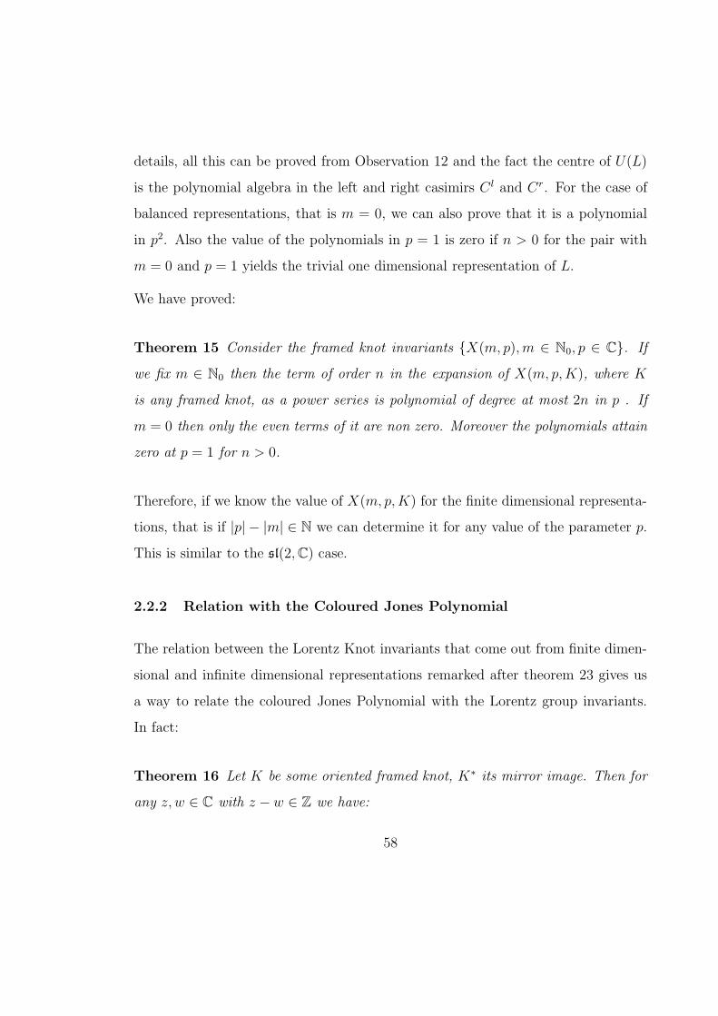
details, all this can be proved from Observation 12 and the fact the centre of U(L)
is the polynomial algebra in the left and right casimirs C l and Cr. For the case of
balanced representations, that is m = 0, we can also prove that it is a polynomial
in p2. Also the value of the polynomials in p = 1 is zero if n > 0 for the pair with
m = 0 and p = 1 yields the trivial one dimensional representation of L.
We have proved:
Theorem 15 Consider the framed knot invariants X(m, p), m ∈ N0, p ∈ C. If
we fix m ∈ N0 then the term of order n in the expansion of X(m, p,K), where K
is any framed knot, as a power series is polynomial of degree at most 2n in p . If
m = 0 then only the even terms of it are non zero. Moreover the polynomials attain
zero at p = 1 for n > 0.
Therefore, if we know the value of X(m, p,K) for the finite dimensional representa-
tions, that is if |p| − |m| ∈ N we can determine it for any value of the parameter p.
This is similar to the sl(2,C) case.
2.2.2 Relation with the Coloured Jones Polynomial
The relation between the Lorentz Knot invariants that come out from finite dimen-
sional and infinite dimensional representations remarked after theorem 23 gives us
a way to relate the coloured Jones Polynomial with the Lorentz group invariants.
In fact:
Theorem 16 Let K be some oriented framed knot, K∗ its mirror image. Then for
any z, w ∈ C with z − w ∈ Z we have:
58
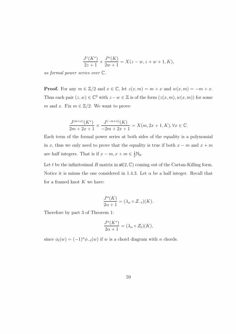
Jz(K∗)
2z + 1× Jw(K)
2w + 1= X(z − w, z + w + 1, K),
as formal power series over C.
Proof. For any m ∈ Z/2 and x ∈ C, let z(x,m) = m + x and w(x,m) = −m + x.
Thus each pair (z, w) ∈ C2 with z−w ∈ Z is of the form (z(x,m), w(x,m)) for some
m and x. Fix m ∈ Z/2. We want to prove:
J (m+x)(K∗)
2m+ 2x+ 1× J (−m+x)(K)
−2m+ 2x+ 1= X(m, 2x+ 1, K), ∀x ∈ C.
Each term of the formal power series at both sides of the equality is a polynomial
in x, thus we only need to prove that the equality is true if both x−m and x+m
are half integers. That is if x−m, x+m ∈ 12N0.
Let t be the infinitesimal R matrix in sl(2,C) coming out of the Cartan-Killing form.
Notice it is minus the one considered in 1.4.3. Let α be a half integer. Recall that
for a framed knot K we have:
Jα(K)
2α+ 1= (λα Z−t)(K).
Therefore by part 3 of Theorem 1:
Jα(K∗)
2α + 1= (λα Zt)(K),
since φt(w) = (−1)nφ−t(w) if w is a chord diagram with n chords.
59

Let K be a framed knot and x be such that α = x − m and β = x + m are half
integers. We have by theorem 5:
Jα(K∗)
2α+ 1× Jβ(K)
2β + 1= (λα Zt)(K)× (λβ Z−t)(K)
= (λα Ztl)(K)× (λβ Z−tr)(K)
= ((λα ⊗ λβ) ZtL) (K).
Recall tL = tl − tr.
Now, λα ⊗ λβ is the central character of the representation ρα ⊗ ρβ of U(L) ∼=U(sl(2,C))⊗ U(sl(2,C)). As we have seen before, this representation is equivalent
to ρ(α − β, α + β + 1) = ρ(m, 2x + 1). Thus their central characters are the same.
This proves
((λα ⊗ λβ) ZtL) (K) = (λm,2x+1 ZtL)(K),
if both x−m and x+m are half integers, and the proof is finished.
We have the following simple consequences.
Corollary 17 Given a framed knot K, then the term of order n in the power series
of X(m, z,K) is a polynomial in m and z
Corollary 18 If O is the unknot, then X(m, p,O) is a convergent power series.
Corollary 19 For balanced representations, that is if m = 0, the invariant X(0, p)
does not distinguish a knot from its mirror image.
Corollary 20 The framed knot invariants X(m, p) are unoriented.
Obviously Theorem 14 also follows from Theorem 16.
60
3 General non compact group knot invariants
We now give a general framework for defining knot invariants from unitary repre-
sentations of Lie Groups, not assumed to be finite dimensional. As we will see the
setting is going to be algebraic at the end.
3.1 Unitary representations and infinitesimal characters
Let G be a Lie group, always assumed to be real, and g be its Lie algebra. Let also
gC = g⊗RC denote the complexification of g. Consider a unitary representation R of
G in the complex Hilbert space V . Notice V is not assumed to be finite dimensional.
We recall that unitarity means that the operator R(g) : V → V is a unitary for any
g ∈ G. Also we suppose a continuity condition, namely that for any v ∈ V the map
g ∈ G 7→ R(g)v ∈ V is continuous.
The main reference for what follows is [Kir]. Let V∞ denote the vector space of
smooth vectors of R. That is
V∞ = v ∈ V : g ∈ G 7→ R(g)(v) ∈ C∞(G, V ). (8)
It is well known that V∞ is dense in V . Differentiating R at the identity of G defines
a map R∞ : g ⊗ V∞ → V . It is possible to show that V∞ is invariant under g and
that R∞ is a honest representation of g. It extends therefore to a representation,
which we also call R∞, of U(gC) in V∞. Recall that V is a complex vector space.
Suppose R is a irreducible representation. In our context this means that V has no
closed invariant subspaces under the action of G. The following (non trivial) result
can be found in [Kir]:
61
Theorem 21 If V is irreducible then any element of C(U(gC)) acts on V∞ under
R∞ as a multiple of the identity operator.
Recall C(U(gC)) denotes the centre of the universal enveloping algebra of gC.
Obviously if V is a finite dimensional complex vector space then the theorem just
stated is a consequence of Schur’s lemma and the unitarity condition is not needed.
Also it is in general possible to show directly that the above property is true for a
large class of infinite dimensional representations, not necessarily unitary. Amongst
them are the representations of SL(2,R) and SL(2,C) which we are going to con-
sider. However the last theorem tells us that our construction is general.
Another way to state Theorem 21 is to say that R has an infinitesimal character.
In other words there exists a (unique) central character χ∞R of U(gC), that is a
morphism of complex algebras C(U(gC)) → C, with the property:
R∞(a)(v) = χ∞R (a)v, ∀v ∈ V ∞, ∀a ∈ C(U(gC)). (9)
Therefore we have the following obvious conclusion (Cf 1.3.3):
Theorem 22 Let G be a real Lie group and R an irreducible unitary representation
of G in some complex Hilbert space V . Let also t be an infinitesimal R-matrix in
the complexification gC of the Lie algebra g of G. There exists a knot invariant with
values in C[[h]]:
I(G, t, R) = χ∞R φt Z. (10)
It has the form
K 7→+∞∑
n=0
χ∞R (φt Zn(K))hn. (11)
62

As an example, consider G = SU(2), thus g = su(2) and gC = sl(2,C). Take t to be
the infinitesimal R-matrix coming from minus the Cartan-Killing form in sl(2,C),
that is < X, Y >= −tr(ad(X) ad(Y )). The tensor t has the form:
t = −1
4(σX ⊗ σX + σY ⊗ σY + σZ ⊗ σZ), (12)
where
σX =1
2
i 0
0 −i
, σY =1
2
0 i
i 0
, σZ =1
2
0 −1
1 0
. (13)
The following is a restatement of Theorem 7:
Theorem 23 Let Jα denote the framed coloured Jones polynomial associated with
the representation Rα of SU(2) with spin α ∈ 0, 1/2, 1, 3/2.... We take the normal-
isation of the coloured Jones polynomial that evaluates at the unknot to the quantum
dimension of the Uh(sl(2,C)) spin α representation. Given any framed knot K we
have:Jα
2α + 1(K) = I(SU(2), t, Rα)(K), α = 0, 1/2, 1, 3/2.... (14)
as formal power series.
3.2 Some examples in the SL(2,R) case
Let us now describe some infinite dimensional examples. Consider the Lie group G =
SL(2,R). It is a non-compact semisimple group. As before we have gC = sl(2,C).
Take again t to be the infinitesimal R-matrix coming from minus the Cartan-Killing
form in gC. We can also write it as
t = −1
4
(
E ⊗ F + F ⊗E +H ⊗H
2
)
, (15)
63

where:
H =
1 0
0 −1
, E =
0 1
0 0
, F =
0 0
1 0
. (16)
We start by defining the representations of SL(2,R) in the principal series. They
depend on an imaginary parameter s ∈ iR and an ε ∈ 0, 1, the parity of the rep-
resentation. In general V s,ε is the space L2(R) of complex-valued square integrable
functions in R. The action of SL(2,R) has the form:
Rs,ε
a b
c d
(f)(x) = sgnε(bx+ d)|bx+ d|s−1f(
ax+ c
bx+ d
)
. (17)
See [GI] for an alternative description of these representations, as well as the defi-
nition of their associated spin network theory. It applies to the construction of spin
foam models for (2 + 1)-Quantum Gravity.
The positive discrete series depends on a parameter m ∈ Z−. The representations
of this type are denoted by Rm,+. The representation space for the representation
Rm,+ is the space of holomorphic functions f in the upper half plane such that:
i
2Γ(−m)
∫
Im(z)>0
|f(z)|2(Im(z))−m−1dzdz < +∞. (18)
The inner product in this Hilbert space has an expression similar to the formula
above. The group SL(2,R) acts in the fashion:
Rs,ε
a b
c d
(f)(x) = (bx+ d)s−1f
(
ax+ c
bx+ d
)
. (19)
The representations in the negative series are denoted by Rm,−. They depend on a
parameter m ∈ Z−. The representation space for them is the space of holomorphic
functions f in the lower half plane such that:
1
2Γ(−m)
∫
Im(z)>0
|f(z)|2|Im(z)|−m−1dzdz < +∞. (20)
64

The action of SL(2,R) in V is similar to the case of the positive discrete series.
The Lie group SL(2,R) still has one more series of unitary representation, namely
the complementary series of representations, and actually some more representations
in the complementary series, now for m > 0. These last are defined as before but
quotienting out invariant spaces of homogeneous polynomials out of them. Details
can be found in [L] or [GGV]. Excluding the representation R0,1, all the repre-
sentations considered are unitary and irreducible. Therefore there is attached to
them a knot invariant with values in C[[h]]. In the next section we relate these knot
invariants to the coloured Jones polynomial.
3.3 The z-Coloured Jones Polynomial as a universal invari-
ant
Let G be a real Lie group, g its Lie algebra and gC the complexification of g. We
suppose gC is equipped with a infinitesimal R-matrix t ∈ gC ⊗ gC. Let also R be a
irreducible unitary representation of G in complex Hilbert space V . A closer look at
the definition of the knot invariant I(G, t, R), cf Theorem 22, tells us that the only
information which we took from the representation R was its infinitesimal character
χ∞R . It is a morphism of algebras from the centre C(U(gC)) of U(gC) to C, that is
a central character of U(gC). In the case gC is semisimple, we know the form of all
such morphisms. Let us say what the situation is in the case gC = sl(2,C). We refer
to [VAR], or to any classical reference on Lie algebras for further details.
The description we are going to give now generalises to any semisimple Lie algebra.
In particular any similar construction of knot invariants out of infinite dimensional
representations of semisimple Lie groups will have the same kind of properties.
65

Consider any Cartan decomposition of sl(2,C) and choose a Borel subalgebra rel-
ative to it. Given a complex number a there exists a unique irreducible, cyclic,
highest weight representation ρa2 of maximal weight a. This representation is finite
dimensional if, and only if, a = 0, 1, 2, .... In this case it integrates to the repre-
sentation of SL(2,C) of spin a2. If a is an arbitrary complex number, any element
of the centre of U(sl(2,C)) acts in the representation space of ρa2 as a multiple of
the identity. Denote by λρa2the central character of ρ
a2 . That is if x is a cen-
tral element of U(sl(2,C)) then λρa2(x) is the unique complex number such that
λρa2(x)v = ρ
a2 (x)(v) for all v in the representation space of ρ
a2 . We will then have
λρa2= χ∞
Ra2, a ∈ 0, 1, 2, ... Recall Rα denotes the representation of SU(2) of spin
α = 0, 1/2, 1, 3/2.... If we consider the usual Cartan decomposition of sl(2,C) then
the irreducible cyclic highest weight representation with highest weight 2z is exactly
the representation ρzof spin z defined in 1.4.6.
All the pieces of the following theorem can be found in [VAR], and almost all the
classical references on Lie algebras.
Theorem 24 Let f : C(U(sl(2,C))) → C be a central character of U(sl(2,C)). We
have:
1. There exists an a ∈ C such that f = λρa2.
2. λρa2= λ
ρb2if and only if (a+ 1)2 = (b+ 1)2.
3. Given x ∈ C(U(sl(2,C))) the map a ∈ C 7→ λρa2(x) is a polynomial in a
of degree smaller or equal to the degree of x in U(sl(2,C)). In fact it is a
polynomial in (a+ 1)2
66
This theorem admits an obvious generalisation to any semisimple Lie algebra.
Notice that the z-coloured Jones polynomial is defined as the form: (cf Theorem 23)
Jz
2z + 1(K) = λρz (φt Z)(K), (21)
here K denotes a framed knot. Due to part 3. of Theorem 24 we can see again that:
Jz
2z + 1(K) =
+∞∑
n=0
Jzn(K)hn =
+∞∑
n=0
(
2n∑
k=0
Jn,k(K)zk
)
hn (22)
Where the degree of (φt Zn)(K) in U(sl(2,C) is not bigger than 2n, for any framed
knot K. Some other properties of the z-coloured Jones polynomial coming from the
corresponding properties of the Melvin-Morton expansion are the following:
1. If K is a framed knot then Jzn(K) is a polynomial in (2z+1)2 of degree smaller
or equal to n.
2. If (2z + 1)2 = (2w + 1)2 then Jz
2z+1= Jw
2w+1.
3. Jz
2z+1is the usual (rescaled) Jones polynomial if 2z + 1 = 1, 2, ....
4. If 2z + 1 = 1,−1, 2,−2... then Jz
2z+1(K) defines a power series in h convergent
in C.
Properties 1, 2 and 3 are easy consequences of our discussion. The fourth is a
consequence of the fact that, in our normalisation, Jz
2z+1(K) is a Laurent polynomial
in eh/4 if 2z + 1 = 1,−1, 2,−2..., as referred in 1.4.2. This generalises to any
semisimple Lie algebra.
67

3.3.1 Some more examples of Melvin-Morton expansions
We now derive some Melvin-Morton expansions from known formulae of the Coloured
Jones Polynomial of some simple knots. These formulae will be useful later.
Let q = exp(h). For an n ∈ N0 and a z ∈ C, consider the term
D(n, z) =n∏
k=1
[
(
q2z+1
2 − q−2z+1
2
)2
−(
qk2 − q−
k2
)2]
. (23)
It is a power series in h such that the first 2n terms are zero. Therefore if f(n), n ∈N0 are power series in h, for example Laurent polynomials in q and q−1, then∑
n∈N0f(n)D(n, z) is an infinite series of power series which is termwise conver-
gent, since it is of terminating type, termwise. Suppose A(z) =∑
n∈N0An(z)h
n
and B(z) =∑
n∈N0Bn(z)h
n are power series whose coefficients depend polynomially
in z, for example power series such as q2z+1
2 or q−2z+1
2 . Then also the coefficients
of their product depend polynomially in z, thus in particular the coefficients of
D(n, z), for any n ∈ N0. The same is true for the coefficients of any power series of
the type∑
n∈N0f(n, z)D(n, z), where f(n, z) ∈ C[[h]] is such that its terms depend
polynomially in z.
Let 31 and 41 denote the zero framed trefoil and figure of eight knots. We have, see
[H]:
Jz
2z + 1(31) =
1
2z + 1
q2z+1
2 − q−2z+1
2
q12 − q−
12
+∞∑
n=0
(−1)nq−n(n+3)/2D(n, z), (24)
Jz
2z + 1(41) =
1
2z + 1
q2z+1
2 − q−2z+1
2
q12 − q−
12
+∞∑
n=0
D(n, z). (25)
In general for any framed knot K there exist Laurent polynomials fn(K)(h), n ∈ N0
68
in q and q−1 such that
Jz
2z + 1(K) = qF (K)z(z+1) q
2z+12 − q−
2z+12
q12 − q−
12
+∞∑
n=0
fn(K)D(n, z), (26)
where F (K) is the framing coefficient of K. Actually, Habiro proved these formulae
only in the case of finite dimensional representations, that for z ∈ 12N0. However
the coefficients of the power series above depend polynomially in z, which implies
the formulae are true also for infinite dimensional representations. This is the old
principle that if two polynomials coincide in an infinite set then they are the same.
We have used this method to prove Theorem 16. We will use it again quite frequently,
in fact in most of all major results we prove. Notice that equation 26 also proves
that Jα
2α+1(K) always defines a Laurent polynomial in q1/4 if α = 0, 1
2, 1, ....
3.3.2 Back to SL(2,R)
Recall the framed knot invariants I(G, t, R) defined in theorem 22. Given that
sl(2,C) is simple, we can prove that any infinitesimal R-matrix in sl(2,C) is a mul-
tiple of the one coming from minus the Cartan-Killing form considered previously,
see 1.3.1. The following result is a straightforward consequence of the discussion
above (especially of Theorem 24):
Theorem 25 Let G be a real form of SL(2,C) and R be an irreducible unitary
representation of G in the Hilbert space V . Let also t be an infinitesimal R-matrix in
sl(2,C). After rescaling t (possibly), there exists a z ∈ C such that I(G, t, R) = Jz
2z+1.
We can prove similar results for any semisimple Lie group.
69

It is possible to find the exact relation between the invariants associated with the uni-
tary representations of SL(2,R) and the z-coloured Jones polynomial which needs
to exist in the light of the theorem above. Let as usual t be the infinitesimal R-
matrix in sl(2,C) coming from minus its Cartan-Killing form. In general the highest
weight representations ρa, a ∈ C of sl(2,C) cannot be integrated to representations
of SL(2,R), however it is possible to relate their central characters with the in-
finitesimal characters of the unitary representations of SL(2,R). We will do it in
5.3. which will prove:
Theorem 26 Let t be the infinitesimal R-matrix in sl(2,C) coming from minus its
Cartan-Killing form. We have, for the principal series of representations:
I(SL(2,R), t, Rs,±1) =J
s−12
s, s ∈ iR, (27)
and
I(SL(2,R), t, Rm,±) =J
m−12
m,m ∈ Z−, (28)
for the discrete series.
Observe that as a consequence the usual Coloured Jones Polynomial can be obtained
out of the unitary infinite dimensional representations of SL(2,R) in the discrete
series.
Another consequence is the fact observed in the introduction that the quantum
knot invariants associated with the infinite dimensional representations SL(2,R)
are in a sense analytic continuations of the ones associated with finite dimensional
representations of the complexification sl(2,C) of sl(2,R). Also the fact that the
non-compact knot invariants are not stronger than the ones associated with finite
dimensional representations. The meaning of this is obvious from the Melvin-Morton
70

expansion (22). Notice however that this property is valid only termwise in the power
series expansions, and we will see later that in some cases the analytically continued
power series may have a zero radius of convergence. This does not happen in the
case of the Coloured Jones polynomial. We will come back to this in Chapter 4.
This property concerning analytic continuations is valid if G is any semisimple Lie
group. I do not know what the answer is in the case of non semisimple Lie algebras.
3.3.3 The Lorentz Polynomial
Recall 2.1. The Lie algebra L ∼= sl(2,C) ⊕ sl(2,C) is the complexification of the
lie algebra of sl(2,C) seen as a real Lie group. As before, consider the infinitesimal
R-matrix tL in LC given by tL = tl − tr. After theorem 16, given z and w in C it is
thus natural to define the Lorentz polynomial as being:
Lz,w
(2z + 1)(2w + 1)(K) =
Jz
2z + 1(K∗)
Jw
2w + 1(K). (29)
Here K is a framed knot and K∗ denotes its mirror image.
Similarly with the SL(2,R) case, we have:
Theorem 27 Let R be a irreducible unitary representation of SL(2,C) in the com-
plex Hilbert space V . There exist z, w ∈ C such that:
I(SL(2,C), tL, R) =Lz,w
(2z + 1)(2w + 1). (30)
Proof. Let f = χ∞R : C(L) → C be the infinitesimal character of R, thus
I(SL(2,C), tL, R) = f φtL Z.
As we have seen in 1.3.4, if K is a framed knot we have
(φtL Z)(K) = (φt Z)(K)⊗ (φ−t Z)(K) ∈ U(sl(2,C))⊗ U(sl(2,C)) ∼= U(L).
71
The central character f : C(U(L)) → C is the central character of a irreducible,
cyclic highest weight representation of U(L). Such representation is the direct sum
of two irreducible cyclic highest weight representations of U(sl(2,C)) of maximal
weights 2w and 2z. They have central characters λρz and λρw , thus f = λρz ⊗ λρz
under the isomorphism C(U(L)) ∼= C(U(sl(2,C)))⊗ C(U(sl(2,C))). In particular
f φtL Z = (λρz φt Z)⊗ (λρw φ−t Z) =Lz,w
(2z + 1)(2w + 1),
for some z and w in C.
As an example let us consider the principal series of unitary representations of
SL(2,C). Their infinitesimal counterpart was defined in 2.1.1. We want to describe
the actual group representations now. For a more geometric description these repre-
sentations in terms of hyperbolic geometry we refer to [GGV]. The unitary principal
series is parametrised by a pair of complex numbers z and w with m = z − w ∈ Z
and iρ = z + w + 1 ∈ iR. In general the parameters m and ρ are referred to as
the minimal spin and the mass of the representation. The ones of minimal spin 0
are the balanced representations of [BC]. As observed in the same reference, they
admit a natural spin network theory. The representation space V for Rm,ρ is L2(C)
and the action of SL(2,C) has the form:
Rz,w
a b
c d
(f)(ξ) = (bξ + d)z−1(bξ + d)w−1f
(
aξ + c
bξ + d
)
. (31)
The representations in the principal series are unitary and irreducible, therefore
there exists a knot invariant attached to them. As before, these knot invariants
are particular cases of the Lorentz polynomial. Since, as referred to in 1.4.6 the
infinitesimal character of R(m, p) is ρ(m, p), we have by Theorem 16:
72
Theorem 28 Let ρ = z + w + 1 and m = z − w we have
I(SL(2,C), tL, Rm,ρ) =
Lz,w
(2z + 1)(2w + 1)= X(m, p). (32)
73
4 Convergence issues
We now look at the analytic properties of the z-coloured Jones polynomial. As we
pointed out for several times before, the power series coming out of it are in general
not convergent (that is they have a zero radius of convergence). We now show this
is what happens at least in the case of torus knots. Later we will have a look at
the properties of the z-coloured Jones polynomial under Borel re-summation. This
is an expanded version of the corresponding chapter of [FM1].
4.1 On the divergence of the z-Coloured Jones Polynomial
power series for torus knots
Let m and p be two coprime positive integers. In what follows Km,p denotes the
(m, p)-Torus Knot, see [Wi1] for example. For each z ∈ C, consider the following
meromorphic function:
Fm,p,z(x) =
sinh(
(2z + 1)√mpx
)
sinh
(
√
mpx
)
sinh(√
pmx)
(2z + 1) sinh(√
mpx) . (33)
Notice it is well defined if 2z + 1 = 0. It is an even function in x. Suppose
2z + 1 ∈ Z \ 0, it is possible to prove that: see [KT]
Jz
2z + 1(Km,p)(h) =
1
2√π
e−h4 (
pm+m
p )
sinh(
h2
)
∫ +∞
−∞e−x
2
Fm,p,z(√hx)dx, ∀h ∈ C. (34)
This is a consequence of a previous formula proved in [Mor]. Notice that for 2z+1 ∈Z \ 0 the power series Jz
2z+1(Km,p)(h) has an infinite radius of convergence. The
origin is never a singular point of Fm,p,z(x) for any z ∈ C, thus if√hx is small
74
enough:
Fm,p,z(√hx) =
+∞∑
k=1
Qm,p,z(k)hkx2k. (35)
In the case 2z+1 ∈ Z\0 the function Fm,p,z(x) is an entire function of exponential
order. That is f is analytic in C and there exist positive constants A and C such
that |Fm,p,z(x)| < AeC|x|, ∀x ∈ C. See 5.4.1. This implies that we have the bound
|Qm,p,z(k)| ≤ D2k/(2k)!, k ∈ 1, 2, ... for some D <∞, by Theorem 52. In practice
this means that, for any h ∈ C, we can interchange the infinite summation with the
integral sign in the following expression:
Jz
2z + 1(Km,p)(h) =
1
2√π
e−h4 (
pm+m
p )
sinh(
h2
)
∫ +∞
−∞e−x
2
(
+∞∑
k=1
Qm,p,z(k)hkx2k
)
dx, ∀h ∈ C,
(36)
valid if 2z+1 ∈ Z\0. This is because all partial sums are bounded by the function
exp(−x2) exp(D|x|√
|h|), which is integrable. Therefore:
Jz
2z + 1(Km,p)(h) =
1
2√π
e−h4 (
pm+m
p )
sinh(
h2
)
+∞∑
k=1
Γ(k +1
2)Qm,p,z(k)h
k, (37)
if 2z + 1 ∈ Z \ 0 and h ∈ C. Given that the coefficients of the Taylor decom-
position of sinh((2z + 1)√mpx) at x = 0 depend polynomially in z we show that
the dependence of the coefficients Qm,p,z(k) in z is in fact polynomial. Thus the
expansion (37) is true for any z ∈ C, now only at the power series level. We have
shown:
Theorem 29 Let m and p be coprime positive integers and Km,p be the (m, p)-torus
knot. The expansion (37) of the z-coloured Jones polynomial of Km,p is correct for
any z ∈ C, as formal power series
75

The functions Fm,p,z(x) have non removable singularities if 2z + 1 /∈ Z \ 0. In
particular there exists a positive constant C such that Qm,p,z(k) > Ck for infinite
k’s. As a consequence we can conclude:
Corollary 30 Let Km,p be the m,n-torus knot. The power series Jz
2z+1(Km,p) has a
zero radius of convergence if 2z + 1 /∈ Z \ 0.
It is easy to conclude that the result above is true also for the mirror images of the
class of torus knots just considered.
It is possible to prove a similar result of divergence in the Lorentz group case: Let
z, w ∈ C. Consider the function
Gm,p,z,w(x) =1
4π
∫ 2π
0
Fm,p,z(x cos(θ))Fm,p,w(ix sin(θ))dθ, (38)
thus if 2z + 1, 2w + 1 ∈ Z \ 0 we have:
Lz,w
(2z + 1)(2w + 1)=
1
sinh(−h
2
)
sinh(
h2
)
∫ +∞
0
e−x2
xGm,p,z,w(x√h)dx, (39)
from (34) If 2z + 1 and 2w + 1 are non zero integers, then Gm,p,z,w is entire of
exponential order. Otherwise it has non removable singularities. For, suppose, for
example, that 2w + 1 /∈ Z \ 0, let w0 be the first singularity of Fm,p,w(ix) in the
positive real line. It is a pole. An explicit calculation tells us that as x approaches
w0 from below along the real line then the first derivative of Gm,p,z,w(x) tends to ∞.
Given any z, w ∈ C, the function Gm,p,z,w(x) is an even function with a zero of order
4 at the origin. Put
Gm,p,z,w(x) =∞∑
k=2
Pm,p,z,w(k)x2k. (40)
76

For fixed k, the dependence of Pm,p,z,w(k) in z and w is polynomial. In fact, if we
fix m, p, z, w (z, w ∈ C then for x small enough the series
Fm,p,x(x cos θ)Fm,p,w(ix sin(θ)) =
∞∑
a,b=0
Qm,p,z(a)Qm,p,w(b)xa+bib cosa(θ) sinb(θ) (41)
converges uniformly for θ ∈ [0, 2π]. Thus
Gm,p,z,w(x) =∑
a,b
Ca,bQm,p,z(a)Qm,p,w(b)xa+b (42)
where
Ca,b =
∫ 2π
0
ib cosa(θ) sinb(θ)dθ. (43)
This proves Pm,p,z,w(k) is a polynomial in z and w for any k. Since Gm,p,z,w(x) is
entire of exponential order if 2z+1, 2w+1 ∈ Z\0, similarly as above, we conclude:
Lz,w
(2z + 1)(2w + 1)=
1
2 sinh(
h2
)
sinh(−h
2
)
+∞∑
k=1
Pm,p,z,w(k)k!hk+1, (44)
from which follows the non-convergence of the power series defined by the Lorentz
polynomial if 2z + 1 or 2w + 1 do not belong to Z \ 0, in the case of torus knots.
We are mainly interested in knot invariants with values in C. As before we refer
to them as numerical knot invariants. It is natural now to ask whether we can
canonically find analytic functions of which the z-coloured Jones polynomial in a
knot are asymptotic developments. In the remainder of this chapter we investigate
this question in the framework of Borel re-summation.
Observation 31 Professor Hugh Morton suggested to me the results by Rozansky
which were conjectured in [R1] and proved in [R2] may provide the framework for
a general proof of the divergence of the z-coloured Jones polynomial, for the case of
knots with a trivial Alexander polynomial.
77
4.2 Borel Re-summation of power series
We make now a brief description of the Borel process of re-summation of power
series. We refer to [SS] for full details and for proofs (which sometimes are not that
simple). The paper [FL] contains a simple and illuminating introduction to this
subject.
4.2.1 Asymptotic power series developments and a lemma due to Borel
Consider a sector Ω = z ∈ C : θ1 ≤ arg(z) ≤ θ2, |z| ≤ C in the complex plane
(or in the Riemann surface of the Logarithm, if θ2 − θ1 ≥ 2π). Let∑+∞
n=0 anhn be a
formal power series which we do not assume to be convergent. Suppose f : Ω → C
is a continuous function in Ω and analytic in the interior int(Ω) of Ω. We say that∑+∞
n=0 anhn is an asymptotic expansion of f at the origin if, for any proper subsector
Ω′ of Ω, and any N = 1, 2..., there exists a positive constant CN such that
∣
∣
∣
∣
∣
f(h)−N∑
n=0
anhn
∣
∣
∣
∣
∣
≤ CN |h|N+1, ∀h ∈ Ω′. (45)
For example the, horribly divergent, series∑+∞
n=0(−1)n(n − 1)!hn is an asymptotic
series for the, perfectly well defined, function h 7→∫ +∞0
e−xh . 1x+1
dx in any sector
Ω = h ∈ C : Re(h) ≥ 0, |h| ≤ C. Here C is a positive constant.
Let Ω be a sector in the complex plane. Denote by G(Ω) the space of holomorphic
function in int(Ω) and continuous in Ω which admit a power series asymptotic ex-
pansion at the origin. It can be proved that G(Ω) is closed under differentiation and
it is an algebra with respect to multiplication of complex functions. If∑+∞
n=0 anhn is
a asymptotic power series expansion of some f ∈ G(Ω) then the coefficients an are
78

unique and can be computed by the formula:
an = limh→0h∈Ω
1
n!f (n)(h). (46)
This permits us to define a map As : G(Ω) → C[[h]]. It can be proved that As is an
algebra morphism and it is well behaved with respect to differentiation. Moreover
it is a surjective map and its kernel is the space of functions analytic in int(Ω) and
continuous in Ω that tend to zero faster than any zn for any n ∈ N. This fact is
known as Borel’s lemma. It permits us to define a re-summation operator of formal
powers series up to functions that go to zero faster that any natural power of z as
z → 0.
In practice, to re-sum a power series means finding an analytic function this power
series is an asymptotic expansion of. Therefore Borel’s lemma tells us that we can
always re-sum them. For practical applications, however, it is important to reduce
as much as possible the uncertainty in the process of re-summation. This is the
subject of the following paragraph.
4.2.2 Power series in the First Gevrey Class and Formal Borel Trans-
forms
Let∑+∞
n=0 anhn be a formal power series. We say that it is of type Gevrey 1 if there
exists a positive constant C such that |an| ≤ Cnn!, ∀n ∈ N. We denote by G1[[h]]
the algebra of formal power series of type Gevrey 1. If Ω is a sector in the complex
plane, then a function in G(Ω) is said to be of type Gevrey 1 if its asymptotic
expansion at zero belongs to G1[[h]]. We also impose that for any subsector Ω′ of Ω
79

there exists a positive C such that∣
∣
∣
∣
f (n)(z)
n!
∣
∣
∣
∣
≤ Cnn!, ∀z ∈ Ω′, ∀n ∈ N.
It is easy to prove that the first condition follows from this last one. Notice that
G1(Ω) is an algebra stable under differentiation.
Suppose the opening of the sector Ω is less than π. Then as before As1 : G1(Ω) →G1[[h]] is a surjective algebra morphism, and its kernel is the space of exponential
decreasing functions in Ω. That is, functions that satisfy the estimate f(h) ≤ Ae−B|h|
for some positive A and B in any proper subsector of Ω.
Recall that the Borel transform B(f) of an analytic function f , if it exists, is the
inverse Laplace transform of it. We refer again to [SS] for a discussion of this subject
in the generality we need. It is well known that B(1) = δ(ξ) and B(hn+1) = ξn/n!.
Notice we do a change of variables h 7→ 1/h in the domain of the Laplace transform.
Let∑
n anhn be a formal power series in the first Gevrey class. Consider the gener-
alised function
F (ξ) = B(+∞∑
n=0
anhn)(ξ) =
+∞∑
n=0
an+1
n!ξn + a0δ(ξ). (47)
It is called the Formal Borel transform of∑+∞
n=0 anhn. Let 0 < a < C be a real
number. Choose a direction eiθ in the complex plane such that Re(eiθ/h) > 0, ∀h ∈Ω. Recall Ω opens less than π. It is possible to prove that the incomplete Laplace
Transform in the direction eiθ:
h 7→ Laeiθ(F (ξ))(h) =∫ aeiθ
0
e−ξh F (ξ)dξ (48)
has∑+∞
n=0 anhn as a power series asymptotic development at the origin. This defines
a re-summation of power series of Gevrey type 1, up to exponentially decreasing
functions.
80
4.2.3 Re-summation Operators
For a better definition of the re-summation operator, we are led to consider formal
power series whose Formal Borel transform can be analytically continued to the
neighbourhood of some ray eiθR+0 in the complex plane, cf [SS]. This will lead to
the definition of a re-summation operator up to rapidly decreasing functions. That
is, functions that verify ∀A > 0, ∃B > 0 : |f(h)| ≤ Be−A/|h|, ∀h ∈ Ω′, in any proper
subsector Ω′ of Ω. In addition it will extend the usual sum of convergente formal
power series.
Let F (ξ) be an analytic function possibly containing a δ(ξ) term, in an open subset
of C containing some ray eiθR+0 . Suppose it grows at most exponentially along it.
The Laplace transform of F (ξ) in the direction eiθ is defined as:
Leiθ(F (ξ))(h) =∫ +∞eiθ
0
e−ξ/hF (ξ)dξ, (49)
whenever the integral is convergent. A lot of properties of this changed Laplace
transform can be deduced from the corresponding ones of the usual Laplace Trans-
form. In particular Leiθ(ξn) = Γ(n+1)hn+1, n = 0, 1, .... If a is a real number bigger
than −1 this generalises to L1(ξa) = Γ(a + 1)ha+1.
Definition 32 (re-summation operators) Let eiθ be a direction in the com-
plex plane and∑+∞
n=0 anhn a formal power series of Gevrey type 1. We say it is
eiθ-summable if its Formal Borel transform can be analytically continued to the
neighbourhood of some ray eiθR+0 , and if its Laplace transform converges in some
nonempty subset of C. If h belongs to the domain of definition of the Laplace trans-
81

form then the eiθ re-summation operator is defined as:
S
(
eiθ,
+∞∑
n=0
anhn
)
= Leiθ(
B(+∞∑
n=0
anhn)(ξ)
)
(h). (50)
We can obviously define the re-summation operators along any curve that tends to
the point at infinity. This re-summation operators are well behaved with respect
to the multiplication of power series. Therefore, to avoid working with generalised
functions, we redefine the re-summation operators and consider:
S(
eiθ,
+∞∑
n=0
anhn
)
=1
hS
(
eiθ,
+∞∑
n=0
anhn+1
)
. (51)
Definition 33 (Borel re-summability) A formal power series∑
n anhn is said
to be Borel re-summable if the re-summation operators S make sense when applied
to it.
4.3 Back to Knots!
Let K be any framed knot. Consider a unitary representation R of SL(2,R). It
is possible to obtain some estimates for the coefficients of the Kontsevich Inte-
gral as well as for the matrix elements of R∞, which are suitable to prove that
I(SL(2,R), t, R) defines a formal power series of Gevrey type 1. This is the subject
of Chapter 6. In fact:
Theorem 34 Let K be a framed Knot, z and w two complex numbers. The series
defined by Jz
2z+1(K) and Lz,w
(2z+1)(2w+1)(K) are of Gevrey type 1. That is, their Formal
Borel Transform defines an analytic function in a neighbourhood of zero.
82

This is probably the most difficult result of this thesis.
Notice equation (37) and Theorem 29 prove this for torus knots since the series∑
kQm,p,z(k)hk has a positive radius of convergence. Recall the set of power series
of Gevrey type 1 is a subalgebra of C[[h]].
We will give a full proof of this theorem in Chapter 6. It is a purely technical proof
and the rest of the thesis is fairly independent of it. In 5.4.2 we prove this theorem
for the Figure of Eight Knot and ”sketch” a possible simple general proof of this
result. We give a condensed proof of it in 5.5, a section extracted from [FM1].
4.3.1 The case of torus knots
We now analyse in detail the properties of the Formal Borel Transform of Jz
2z+1(K)
in the case in which K is a torus knot. We shall see the re-summation operators
make sense in this case. The ambiguity in the process of re-summation is reduced
to a finite set of functions differing by rapidly decreasing functions. The main idea
is that equation (34) is almost a Laplace transform. In fact if we make the change
of variables x 7→ √x/
√h we can write it has:
Jz
2z + 1(Km,p)(h) =
1
4√π
e−h4 (
pm+m
p )
sinh(
h2
)
1√h
∫ +∞
0
e−x/hFm,p,z2√x(√x)dx, ∀h ∈ R+. (52)
Compare with (49). Notice that the right hand side of this equation also makes
sense if z ∈ C and h is small enough. This will actually be our re-summation if
h ∈ R+. Obviouly, some details are in need:
Let f and g be two complex valued functions continuous in some open subset of C
which contains 0. Recall that their convolution is defined as
(f ∗ g)(x) =∫ x
0
f(x− ξ)g(ξ)dξ, (53)
83

whenever it makes sense. The contour of integration is chosen to be the segment
connecting 0 and x. If f and g are entire then their convolution is an entire function.
It is well know that if f and g grow at most exponentially along a ray eiθ then the
same is true for their convolution, and in addition Liθ(f ∗g)(h) = Liθ(f)(h)Liθ(g)(h)whenever all transforms makes sense. Suppose f and g are meromorphic functions
which do not have the origin as a singular point. Let D(f, g) be the set of points
in C that can be connected to the origin by a straight line which does not pass by
any singularity of f or g. The convolution of f and g is an analytic function in
D(f, g). The singularities of f ∗ g are in general ramifying due to the fact f and g
may have non zero residua at their singular points. One can easily determine the
Taylor series of f ∗ g in zero from the Taylor series of f and g, in fact if f(x) =∑+∞
n=0 fnxn and g(x) =
∑∞n=0 gnx
n then (f ∗ g)(x) =∑∞
n,m=0m!n!
(m+n+1)!fmgnx
m+n+1,
which converges whenever the Taylor series of f and g converge. This is because,
in general, xm ∗ xn = m!n!(m+n+1)!
xm+n+1;m,n ∈ N, apart from some simple analysis,
basically the principles that a power series converges uniformly in any compact set
contained in its disk of convergence, this disk being the maximal disk that does not
contain any singularity. In particular if the coefficients of the Taylor series of fz(x)
and gz(x) at zero depend polynomially in z then the same is true for the coefficients
of the Taylor series of f ∗ g. This fact will have prime importance in the sequel.
Suppose f is an odd meromorphic function non singular at the origin. Then the
convolution 1/√x ∗ f(√x) defines an analytic function in D(f), where D(f) is the
set of points in the complex plane that can be connected to zero by a straight
line whose square does not meet any singularity of f . Notice D(f) contains a
neighbourhood of 0. In fact if f(x) =∑+∞
n=0 anx2n+1 in a neighbourhood of the
origin then 1/√x ∗ f(√x) =∑∞n=1
Γ(1/2)Γ(n+1+1/2)Γ(n+2)
anxn, in the same neighbourhood.
84

As before, the singular points of 1/√x ∗ f(√x) are usually ramifying due to the
residua of f . Consider
Im,p,z =Γ(1
2)−1√x
∗ Fm,p,z(√x)
2√x
. (54)
Thus if 2z + 1 ∈ Z \ 0 then Im,p,z(x) is an entire function of exponential order.
Moreover, by (52) we have
1
2√π
e−h4 (
pm+m
p )
sinh(
h2
) L1(Im,p,z(x))(h) =Jz
2z + 1(Km,p)(h), h > 0. (55)
In general for any z ∈ C, the function Im,p,z(x) is meromorphic, but it is well defined
in a neighbourhood of zero. In addition the Taylor coefficients of Im,p,z depend
polynomially in z, since the same is true for the Taylor coefficients of Fm,p,z(x) in 0,
as we have seen before. Let
Hm,p,z(x) = B(
h
2√π
e−h4 (
pm+m
p )
sinh(
h2
)
)
. (56)
It is an entire function of x. In fact it is a function of exponential order, the type
(see 5.4.1) of which is smaller than 1/π + ε, where ε > 0 is arbitrary. We can see
it from the fact its Taylor coefficients are given by 1(n−1)!an where
∑
n anhn has a
radius of convergence equal to π. The Laplace transform in any direction always
exists for h small enough. It extends analytically back the original function. This
follows from the known principle that we can take the Laplace transform term by
term in the power series developments of exponential order functions. We can prove
it from the fact |f (n)(0)| ≤ Cn, ∀n, see 5.4.1.
Suppose m and p be coprime positive integers and let Km,p denote the (m, p)-Torus
knot. From equation (55), it is immediate that if 2z + 1 ∈ Z \ 0 we have
hJz
2z + 1(Km,p))(h) = L1
(
Hm,p,z(x) ∗ Im,p,z(x))
(h), h ∈ (0, 1/π) (57)
85

Notice that Hm,p,z(x) is exponential of type 1/π. Thus by the unicity theorem for
Laplace transforms it follows that
B(
hJz
2z + 1(Km,p)
)
(x) = Hm,p,z(x) ∗ Im,p,z(x), ∀x ∈ C, 2z + 1 ∈ Z \ 0. (58)
We also need to use the fact that we can take the Laplace transform term by term
in the Taylor expansion of Im,p,z(x) at zero to prove this. But this follows from the
fact this function is of exponential order if 2z + 1 ∈ Z \ 0.
Now Hm,p,z(x) ∗ Im,p,z(x) is a z-dependent family of analytic functions in a neigh-
bourhood of zero, whose Taylor series coefficients in zero depend polynomially in z.
In particular, equation (58) is true in the power series level. Therefore:
Theorem 35 Let m, p be coprime integer and Km,p the (m, p)-torus Knot. The
formal Borel tranform of Jz
2z+1(Km,p)) extends analytically to the function Hm,p,z(x)∗
Im,p,z(x), well defined in C \ (−∞, π2/(mp)].
Suppose 2z+1 is not a non zero integer. Then the singularity of Hm,p,z(x)∗Im,p,z(x)in −π2/(mp) is ramifying, since the singularity of Fm,p,z in iπ/
√mp has an non zero
residue. Therefore we cannot remove it. This tells us that we cannot refine the
estimate in Theorem 34.
In addition we can say that Hm,p,z(x) ∗ Im,p,z(x) grows at most exponentially along
any ray different of R−. Since the type of Hm,p,z(x) as an exponential function is
1/π, and Im,p,z(x) grows slower than Aeε|z| for any ε > 0, this rate of exponential
growth of Hm,p,z(x) ∗ Im,p,z(x) can be taken smaller than 1/π + ε for any ε > 0.
We summarise our discussion and add some more simple facts:
Theorem 36 Let m and p be coprime positive integers and Km,p be the (m, p)-Torus
Knot. Let z be a complex number such that 2z + 1 /∈ Z \ 0
86

1. The Formal Borel transform of h Jz
2z+1(Km,p) extends to an analytic function in
C \ (−∞, π2/(mp)]
2. The singularity in −π2/(mp) is a ramification point
3. If eiθR+0 is a ray in the complex plane that is not the set of non-positive
real numbers then B(h Jz
2z+1(Km,p))(x) grows not faster than Ae
|x|/(π−ε) along it
where ε > 0 is arbitrary. This constant A can be chosen independent of the
direction chosen.
It is now very easy to analyse the re-summation of the z-coloured Jones polynomial
for torus knots. Recall definition 32 and the comments after. Let B(π) = h ∈C, |h| < π. If h ∈ B(π) consider D(h) = w ∈ S1 \ −1 : Re(w/h) > 1/π 6= ∅.Given h ∈ B(π) then D(h) is connected if Re(h) ≥ 0 and it has two connected
components otherwise.
Suppose Re(h) ≥ 0. Given that D(h) only has one connected component, the re-
summation S(w, h Jz
2z+1(Km,p)(h)) does not depend on w ∈ D(h). This follows from
point 3 of the previous theorem and Cauchy’s integral formula. In addition, if 2z+1
is a real or an imaginary number, the re-summation takes positive real values of h
to real numbers, this is because the Borel transform is real in this case. Notice the
last case corresponds to the representations of SL(2,R) in the principal series.
Due to the fact that D(x) has two connected components if Re(x) < 0 the same is
not true in this case. In fact if x is a real number smaller than 0 the two different
re-summations will give conjugated complex numbers of non zero imaginary part
for the case 2z + 1 is real or imaginary. This is obvious from the fact the Borel
transform is real. Notice that the values of the re-summation, as well as the possible
87

ambiguities can be read directly from equation (34).
The case of the mirror images of torus knots considered can be treated in a similar
way. We just need to take the mirror image in the previous description. Therefore,
for these knots the domain of re-summation is also B(π). The re-summation proce-
dure having 2 branches if Re(h) > 0 and one otherwise. As before, the real parts of
the re-summation for real h, are independent of the re-summation procedure if we
stick to representations in the principal series.
The Lorentz group case can be dealt with considering the fact L1(f(x)′)(h) =
1/hL1(f(x))(h)− f(0), thus
B(
hLz,w(2z + 1)(2w + 1)
(Km,p)
)
(x)
= B(
hJz
(2z + 1)(K∗m,p)
)
(x) ∗ d
dxB(
hJw
(2w + 1)(Km,p)
)
(x)
This is thus a well defined function in C \ ((−∞,−π2/(mp)] ∪ [π2/(mp),+∞)). It
grows exponentially along any ray not contained in R. Therefore, the domain for
the re-summation of Lw,z
(2z+1)(2w+1)(Km,p) is again B(π). Unless h is imaginary, we now
have always two branches for re-summation, if 2z + 1 and 2w + 1 are not non zero
integers. Therefore
Theorem 37 Let Km,p be the (m, p)-torus knot. For any z, w ∈ C the power series
Jz
2z+1(Km,p)(h) and
Lz,w
(2z+1)(2w+1)(Km,p)(h) are Borel re-summable.
Recall that the process of Borel re-summation is well behaved with respect to the
multiplication of power series. Therefore we can calculate the re-summation of the
Lorentz Polynomial, including its ambiguities, out of the re-summation of the z-
Coloured Jones Polynomial.
88
4.4 Conclusion to chapters 1, 2, 3 and 4
Let G be any real Lie group. As we have seen, if we are given an ad-invariant non
degenerate symmetric bilinear form in g⊗R C, there exists a framed knot invariant
φt Z with values in the algebra of formal powers series in h over the centre of the
universal enveloping algebra of g⊗R C, in other words is is a formal power series of
differential operators in G. If g ⊗R C is a semisimple Lie algebra and V is a finite
dimensional representation of G then this formal power series at a particular value
of h evaluates to an operator, or h-dependent family of operators, V → V , which
is a G-intertwiner. The trace of these operators will yield the usual quantum group
knot invariants.
Instead of trying to make sense of this power series of differential operators at a
particular value of h for the case V is an infinite dimensional representation, it
is observed that each term of this power series acts as a multiple of the identity
operator in the space of smooth vectors of any unitary irreducible representation.
Therefore φt Z can be evaluated in any representation of this type. This gives us
a knot invariant with values in the algebra of formal power series over C for any
unitary irreducible representation of G. At least in the case g is semisimple these
knot invariants express out of the knot invariants associated with finite dimensional
representations of the quantised universal enveloping algebra Uh(g) by a analytic
continuation in the power series level, see theorem 26 and the comments after.
Notice that a coherent way of realising this analytic continuation at the level of the
values of the quantum group invariants would give us a way of defining C-valued
knot invariants associated with infinite dimensional unitary representations.
However, at least in the case G = SL(2,R) or G = SL(2,C), for some interesting
89

infinite dimensional unitary representations the power series that we obtain have
zero radius of convergence. The process of Borel re-summation is analysed in the
case of the z-coloured Jones polynomial. It is observed that in this case the power
series are of Gevrey type 1, which means their Formal Borel Transform defines an
analytic function in a neighbourhood of zero. In particular we can define a re-
summation operator apart from exponentially decreasing terms, for example from
expression (48). However for the Borel re-summation procedure to be applied in
full generality, we need the extra conditions that the formal Borel transform can be
analytically continued to some ray eiθR+0 admitting a Laplace transform with a non
zero domain along this direction. This reduces the uncertainty in the re-summation
to a numerable set of functions differing by rapidly decreasing terms. It is verified
that this is indeed what happens when considering torus knots. Namely the formal
Borel transform can be continued along mostly all directions. The singularities of it
are ramifying, and the result of re-summation can have at most two branches, both
solutions of the problem of analytically extending the values of the coloured Jones
polynomial to complex spins. In general for representations in the principal series
with real h the two branches define conjugated complex numbers. The question that
arises naturally concerns the behaviour of the z-coloured Jones polynomial in the
general case, namely:
1. Can the Formal Borel Transform of Jz
2z+1(K) be analytically continued in gen-
eral?
2. Does it admit Laplace transforms with non zero domain?
3. Which kind of ambiguities will result from this process of re-summation?
90

4. Do these ambiguities have a geometric meaning7? For example which geo-
metric object corresponds to the residue, if any, of the first singularity of the
formal Borel Transform of the z-coloured Jones polynomial.
5. Can we generalise all this to links?
These open problems start a totally new direction in quantum group theory with
wide applications to mathematical physics.
7I must thank Professor Laurent Fredeil for opening my eyes to this
91
5 Appendix to chapters 1, 2, 3 and 4
5.1 Proof of Theorem 2
This is a known result, first referred to by Kontsevich in his memorable article
[Ko]. Let g be a Lie algebra and U(g) be its universal enveloping algebra. Let also
∆ : U(g) → U(g)⊗ U(g) be the comultiplication map. It is a coassociative algebra
morphism which verifies ∆(X) = X ⊗ 1 + 1 ⊗ X, ∀X ∈ g. For any integer n ≥ 0,
we define ∆(n) : U(g) → U(g)⊗(n+1) as being the nth-iterate of ∆. In other words:
∆(0) = id, ∆(1) = ∆, ∆(2) = (∆⊗ id)∆, by coassociativity this equals (id⊗∆)∆.
In general we have ∆(n+1) = (∆⊗ id)∆(n). All iterates of ∆ are algebra morphisms.
It is easy to verify that:
∆(n)(X) = X ⊗ 1⊗n−1 + 1⊗X ⊗ 1⊗n−2 + ... + 1⊗n−1 ⊗X,X ∈ g. (59)
The Hopf algebra U(g) is cocommutative. For a permutation σ ∈ Sn, let τs :
U(g)⊗n →: U(g)⊗n be the obvious permutation morphism. From equation (59) it is
trivial that τσ ∆n(X) = ∆n(X) for any permutation σ and X ∈ g. Therefore:
Lemma 38 For any permutation σ ∈ Sn we have τσ ∆(n) = ∆(n).
This is also true for any X ∈ U(g) since U(g) is generated by g as an algebra.
Definition 39 Let g be a Lie algebra. We define U(g)⊗ng as
U(g)⊗ng = a ∈ U(g)⊗n : [a,∆(n)(X)] = 0, ∀X ∈ U(g).
The tensors in U(g)⊗ng will be called g-invariants.
92

Notice that U(g)⊗ng is the centre of U(g) for n = 1. Obviously U(g)⊗ng is a subalgebra
of U(g)⊗n. In addition, since U(g) is generated by g, as an algebra we have
U(g)⊗ng = a ∈ U(g)⊗n : [a,∆(n)(X)] = 0, ∀X ∈ g.
Define m : U(g)⊗n → U(g) by x1 ⊗ x2 ⊗ ...⊗ xn 7→ x1x2...xn.
Lemma 40 If a ∈ U(g)⊗ng then m(a) is central in U(g)
Proof. Let X ∈ g and a ∈ U(g)⊗ng . We have ∆(n)(X)a = a∆(n)(X), where
a = a1 ⊗ a2 ⊗ ... ⊗ an, since a is g-invariant; thus m(∆(n)(X)a) = m(a∆(n)(X)).
From equation (59), the last equality implies Xa = aX , where X ∈ g. Therefore,
the result follows from the fact U(g) is generated by g as an algebra.
Lemma 41 For a tensor t =∑
k ak⊗bk ∈ U(g)⊗U(g) and i < j ≤ n let ti,j denote
the tensor of U(g)⊗n obtained by inserting t in the ith and jth variables and 1 in the
others. Suppose t ∈ U(g)⊗ U(g) is g-invariant. Then ti,j is also g-invariant
Proof. Let σ be a permutation sending 1 to i and 2 to j. For any X ∈ U(g) we
have, by Lemma 38:
[∆(n)(X), ti,j] = τσ [∆(n)(X), t1,2] = τs [(∆⊗ id) ∆(n−1)(X), t⊗ 1] = 0.
Therefore
93

Proposition 42 Let ω be a chord diagram with n chords and t an infinitesimal
R-matrix. Chose an initial point p on the circle to evaluate φt,p(w). This element
is central in U(g)
Proof. Trivial from the fact φt(ω) = m(∏n
k=1 tik,jk), since an infinitesimal R-matrix
is always g-invariant. Notice that the set of g-invariant tensors is always an algebra.
We now prove that φt,p(ω) does not depend on the initial point p in the circle. Let
4Tp be the 4T relations now understood modulo isotopies of the circle fixing p. We
have already observed in 1.3 that:
Lemma 43 Let p be an initial point on the circle. The map ω 7→ φt,p(ω) satisfies
the 4T relations.
This is actually a consequence of equation (1). We now need to prove that moving
p around the circle and passing through an endpoint of a chord is a consequence of
the 4Tp-relations. This will also prove that the multiplication of two chord diagrams
does not depend on the point in which we break the circles. This argument appears
in several places, for example [K] and [BN]. We show that the move in figure 8 is
a consequence of the 4Tp-relations. Call the chord diagram on the left ω and the
chord diagram on the right w′. We now understand chord diagrams modulo isotopy
fixing p. To this end, let d be a chord of w different of c. Define wd as in figure 9.
In particular wd = 0 modulo the 4Tp relations. But obviously
∑
d∈ωd6=c
wd = w − w′
modulo isotopy fixing p. This finishes the proof the φt,p(ω) does not depend on p.
The rest of the proof of theorem 2 is trivial.
94
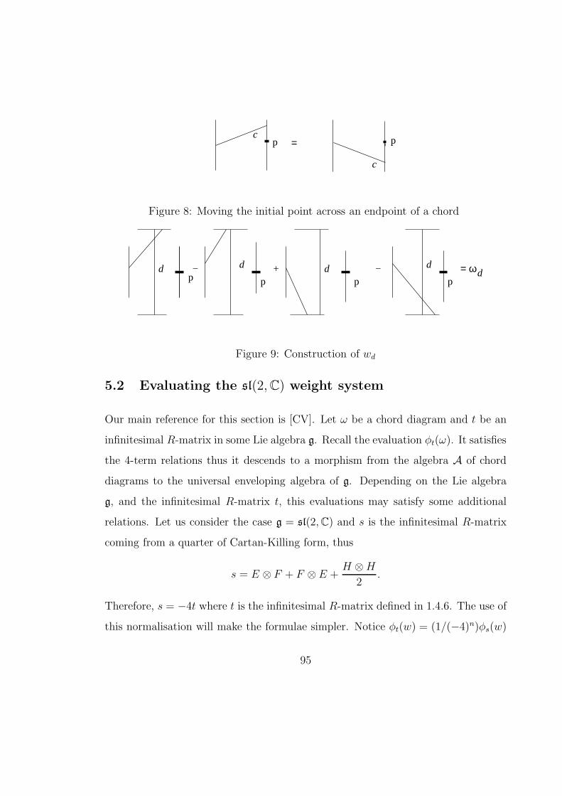
p p=c
c
Figure 8: Moving the initial point across an endpoint of a chord
pd d
pd
p
d− + − dωp
=
Figure 9: Construction of wd
5.2 Evaluating the sl(2,C) weight system
Our main reference for this section is [CV]. Let ω be a chord diagram and t be an
infinitesimal R-matrix in some Lie algebra g. Recall the evaluation φt(ω). It satisfies
the 4-term relations thus it descends to a morphism from the algebra A of chord
diagrams to the universal enveloping algebra of g. Depending on the Lie algebra
g, and the infinitesimal R-matrix t, this evaluations may satisfy some additional
relations. Let us consider the case g = sl(2,C) and s is the infinitesimal R-matrix
coming from a quarter of Cartan-Killing form, thus
s = E ⊗ F + F ⊗ E +H ⊗H
2.
Therefore, s = −4t where t is the infinitesimal R-matrix defined in 1.4.6. The use of
this normalisation will make the formulae simpler. Notice φt(w) = (1/(−4)n)φs(w)
95
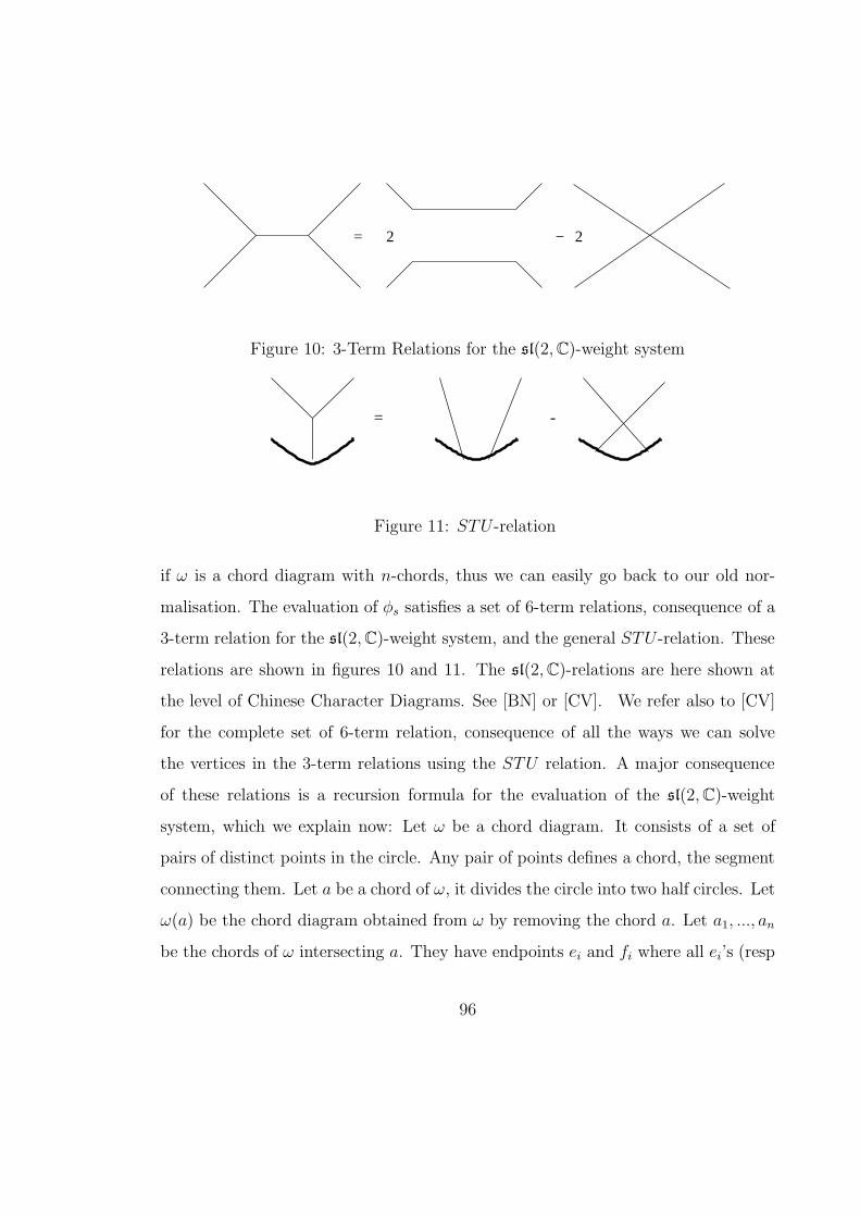
= 2 2−
Figure 10: 3-Term Relations for the sl(2,C)-weight system
= -
Figure 11: STU -relation
if ω is a chord diagram with n-chords, thus we can easily go back to our old nor-
malisation. The evaluation of φs satisfies a set of 6-term relations, consequence of a
3-term relation for the sl(2,C)-weight system, and the general STU -relation. These
relations are shown in figures 10 and 11. The sl(2,C)-relations are here shown at
the level of Chinese Character Diagrams. See [BN] or [CV]. We refer also to [CV]
for the complete set of 6-term relation, consequence of all the ways we can solve
the vertices in the 3-term relations using the STU relation. A major consequence
of these relations is a recursion formula for the evaluation of the sl(2,C)-weight
system, which we explain now: Let ω be a chord diagram. It consists of a set of
pairs of distinct points in the circle. Any pair of points defines a chord, the segment
connecting them. Let a be a chord of ω, it divides the circle into two half circles. Let
ω(a) be the chord diagram obtained from ω by removing the chord a. Let a1, ..., an
be the chords of ω intersecting a. They have endpoints ei and fi where all ei’s (resp
96

a
aa
=ω =ω(a)
=ω||
ij
ei
fi
ej
ej
e
e
e
f
f f
fj
f j
j
f
ei =ω
X
j
i
f i
i
j
i
i
je
(a,i,j) (a,i,j)
Figure 12: Diagrams appearing in the recursive relation for the sl(2,C)-weight sys-
tem
fi’s) belong to the same half circle. Let ai and aj be two distinct chords intersecting
a. We define w||(a, i, j) (resp wX(a, i, j)) as being obtained from w(a) by removing
a and ai, and inserting two chords connecting ei to ej and fi to fj (resp ei to fj and
ej to fi ). See figure 12. Recall ⊖ stands for the chord diagram with only one chord.
Theorem 1 of [CV] tells us:
Theorem 44 (Recursive Relation for sl(2,C)-weight system) Let w be a
chord diagram and a be a chord of it. Let also a1, .., an be the chords of ω intersecting
a. We have:
φs(ω) = φs
(
(⊖− 2n)ω(a) + 2∑
1≤i<j≤n(ω||(a, i, j)− ωX(a, i, j))
)
97

5.3 Proof of Theorem 26
The main results for the proof of this theorem appear in [L] VI.§5.
Consider the following elements of sl(2,R)⊗R C ∼= sl(2,C):
W =
0 1
−1 0
, E− =
1 −i−i −1
, E+ =
1 i
i −1
. (60)
Thus they are a basis of sl(2,C) and satisfy the commutation relations:
[E+, E−] = −4iW, [W,E+] = 2iE+, [W,E−] = −2iE−. (61)
Consider
H0 =⊕
n∈Zspanu2n, H1 =
⊕
n∈Zspanu2n+1.
Let s ∈ C, consider the representations r(s, 0) and r(s, 1) of sl(2,C) in H0 and H1,
respectively, such that:
Wun = inun, E−un = (s+ 1− n)un−2, E+un = (s+ 1 + n)un+2. (62)
Lemma 45 For any s ∈ C and ε ∈ 0, 1, the representation r(ρ, ε) have a central
character c(s, ε). In other words, any element X of the centre C(U(sl(2,C))) → C
acts in then as a multiple c(s, ε)(X) of the identity.
Notice the representations r(s, ε) are not always irreducible.
Proof. Suppose first that s ∈ C \ Z. Let f : Hε → He be an intertwiner, we
show that it needs to be a multiple of id. This will prove that r(s, ε) has a central
character. Let f(un) =∑
k Aknuk. Since f W = W f we have:
in∑
k
Aknuk =∑
k
ikAknuk, ∀n =⇒ i(n− k)Akn = 0, ∀n, k.
98
In particular Akn = 0 if k 6= n. Let us now show that Ann = An+2n+2, ∀n. Given that
f E+ = E+ f , yields (s+1+n)Ann = (s+1+n)An+2n+2, thus, since s /∈ Z, we must
have Ann = An+2n+2, ∀n. For the general case, consider the matrix elements:
Ms,ε(X, k, n) = 〈un|r(s, ε)(X)|uk〉 ,
where X ∈ U(sl(2,C)). Then obviously Ms,ε(X, k, n) is a polynomial in s if k, n, ε
andX are fixed. IfX ∈ C(U(sl(2,C))) thenMs,ε(X, k, n) = δ(k, n)c(s, ε)(X) for s ∈C \ Z, where c(s, ε)(X) is a polynomial in s, uniquely determined. In particular we
must also have Ms,ε(X, k, n) = δ(k, n)c(s, ε)(X) for s ∈ Z and X ∈ C(U(sl(2,C))).In other words
r(s, ε)(X) = c(s, ε)(X)id, ∀X ∈ C(U(sl(2,C))), ∀s ∈ C, ∀ε ∈ 0, 1,
where c(s, ε)(X) is a polynomial in s.
Suppose s = m, where m is a positive odd integer. Then the representation r(m, 0)
has two invariant subspaces, namely
H0(≤ −(m+ 1)) =⊕
n∈≤−(m+1)n is even
spanun and H0(≥ (m+ 1)) =⊕
n∈≥(m+1)n is even
spanun.
We thus have representations r(m, 0,≤) and r(m, 0,≥) of sl(2,C) inH0(≤ −(m+1))
and H0(≥ (m+ 1)) for any odd m. Let
H0(m)fin =H0
H0(≤ −(m+ 1))⊕H0(≥ −(m+ 1)),
then r(m, 0) descends to a finite dimensional representation r(m, 0)fin of sl(2,C)
in it. As in lemma 45 one proves it is irreducible, for any intertwiner must be a
multiple of id. Therefore r(m, 1)fin is the representation of sl(2,C) of spin (m−1)/2
99
since H0(m)fin has dimension m. Obviously, all representations r(m, 0)fin, r(m, 0,≤)
and r(m, 0,≥) have central characters and they are all equal to c(m, 0). This is a
consequence of Lemma 45.
Let λz be the central character of the representation of sl(2,C) of highest weight
2z, in other words of the representation of sl(2,C) of spin z, where z is a complex
number. The last observations prove immediately that c(m, 0) = λ(m−1)/2 if m is a
positive odd integer, since both equal the central character of the representation of
sl(2,C) in H0(m)fin. Let X ∈ C(U(sl(2,C))), thus both c(s, 0)(X) and λ(s−1)/2(X)
are polynomials in s. Since they coincide for m ∈ 1, 3, 5, .. we have proved
Lemma 46 c(z, 0) = λ(z−1)/2, ∀z ∈ C
We prove analogously:
Lemma 47 c(z,−1) = λ(z−1)/2, ∀z ∈ C
The following theorem is shown in [L].
Theorem 48 Let s ∈ iR and ε ∈ 0, 1. The representations r(s, e) is a sub-
representation of R∞s,ε, the representation of sl(2,C) in the space of smooth vec-
tors of Rs,ε. If m is an odd negative integer, then the representation r(m, 0,≥)
(resp r(m, 0, leq) is a subrepresentation of R∞m,+ (resp R∞,m,−), and analogously
for r(−m,−1,≥) and r(−m,−1,≤) if m is an even negative integer.
Theorem 26 now follows easily.
100
5.4 Entire functions of exponential order and proof of The-
orem 34 for the Figure of Eight Knot
5.4.1 Power series developments of functions of exponential order
All the material presented here can be found in mostly all books of advanced complex
analysis. My favourite one is [CH].
Definition 49 Let f : C → C be an entire function, in other words a function
analytic in C. Then f is said to be of exponential order if there exist B,C < ∞such that
|f(z)| ≤ B exp(C|z|), ∀z ∈ C.
Definition 50 Let f be an entire function of exponential order. The function f is
said to be of type C > 0 if we can find B <∞ such that
|f(z)| ≤ B exp(C|z|), ∀z ∈ C.
Therefore, if f and g are two functions of exponential order of type A and B, then
also f+g and fg are of exponential order of types max(A,B) and A+B, respectively.
Obvioulsly the functions sinh(Az), cosh(Az) or exp(Az) are all of exponential order
and of type A. If n is integer and A ∈ C, then
sinh((n+ 1)Ax)
sinh(Ax)=
n∑
k=−nexp(Akx),
which proves that Fm,p,z(x) (see 4.1) is an entire function of exponential order if
2z + 1 is a non zero integer.
101
An easy application of Cauchy’s integral formula is the following known fact about
entire functions: Let f be an entire function. Put
f(z) =
∞∑
n=0
anzn. (63)
Lemma 51 (Cauchy’s Inequality) Let f be an analytic function in a neighbour-
hood of the origin in C. If f(z) ≤ M in the circle of radius R around the origin.
We have
|an| ≤M
Rn, ∀n ∈ N.
Therefore
Theorem 52 Suppose f is an entire function such that |f(z)| ≤ A exp(Cz), for
some A,C > 0. Then the coefficients of (63) satisfy
an ≤ ACn en
nn, ∀n ∈ N,
thus from Lemma 72 (consequence of Stirling Inequalities 93), we can find D < ∞such that
|an| ≤Dn
n!, ∀n ∈ N.
This constant D can be taken as close to C as we want. This is obvious from Stirling
Inequalities.
Proof. See [CH] page 254. By Cauchy’s Inequalities we have
|an| ≤ Aexp(CR)
Rn, ∀n ∈ N,
for any R > 0. Thus
|an|1/n ≤ A1/nexp(CR/n− ln(R)), ∀R > 0, ∀n ∈ N.
102
The minumum, which obviously exists since C > 0, of CR/n − ln(R) when R > 0
is attained in R = n/C. In particular
|an|1/n ≤ A1/n 1
neC, ∀n ∈ N,
which implies
|an| ≤ ACn en
nn, ∀n ∈ N.
5.4.2 Proof of the Theorem 34 For the Figure of Eight Knot
Recall that the z-Coloured Jones Polynomial for the zero framed Figure of Eight
Knot is
Jz
2z + 1(41) =
1
2z + 1
q2z+1
2 − q−2z+1
2
q12 − q−
12
+∞∑
n=0
D(n, z).
where
D(n, z) =
n∏
k=1
[
(
q2z+1
2 − q−2z+1
2
)2
−(
qk2 − q−
k2
)2]
.
and q = exp(h). See 3.3.1. Let us prove it is a power series of Gevrey type 1. To
make the notation simpler, we only analyse the case 2z+1 = 0. The general case is
totally similar. Notice that at z = 0 we attain an infinite dimensional representation
of SL(2,R), see Theorem 26. Since the set of power series of Gevrey type 1 is a
subalgebra of C[[h]] it suffices to prove that
∞∑
N=0
cNhN =
∞∑
n=0
(−1)n22nn∏
m=1
sinh2
(
mh
2
)
(64)
103

is a power series of Gevrey type 1. Notice this power series only has even terms. Let
FN(h) =
N/2∑
n=0
22n(−1)nn∏
m=1
sinh2
(
mh
2
)
,
thus obviously CN = aN where aN is the N th order term of the Taylor expansion
(63) of FN(h) at h = 0. We now wish to apply Theorem 52 to FN . For any h ∈ C
we have | sinh(Ah)| ≤ exp(A|h|), h ∈ C. Thus for any h ∈ C we have:
|FN(h)| ≤N/2∑
n=0
22nn∏
m=1
exp(m|h|)
=
N/2∑
n=0
22n exp
(
n(n+ 1)
2|h|)
≤(
N
2+ 1
)
2N exp
(
N(N + 2)
8|h|)
.
In particular, by theorem 52 we have
|aN | ≤(
N
2+ 1
)
2N(
N(N + 2)
8
)NeN
NN≤ CNNN ,
where C does not depend on N . Therefore by Lemma 72 there exists a D <∞ such
that
|CN | = |aN | ≤ DNN !, ∀N ∈ N0
this proves Theorem 34 for the Figure of Eight knot.
The same kind of argument would yield a similar result for the Trefoil knot, see
3.3.1. Even though equation (37) and Theorem 29 have already given a proof of it.
In fact we can prove:
Theorem 53 Let K be a framed knot. Consider Habiro’s general expression (26)
for the z-Coloured Jones Polynomial of it as in 3.3.1. Suppose that the exists A
104

and B such that for any integer n the function fn(K)(z) is an entire function of
exponential order for which:
|fn(K)(z)| ≤ A exp(Bn2|z|), ∀z ∈ C, ∀n ∈ N0.
Then Jz
2z+1(K)(h) is a power series of Gevrey type 1.
Therefore with a better knowledge of the coefficients of Habiro’s formula (26) we
may prove Theorem 34 in full generality and in a simple way. This would avoid the
complicated and especially very techical approach for it in chapter 6.
5.5 Condensed proof of Theorem 34
This is extracted from [FM1]. Chapter 6 is an expanded version of this section with
full proofs.
We assume that the reader is familiar with the construction of the Kontsevich In-
tegral, as well as the algebraic structure in the space of chord diagrams. See for
example [BN], [Wi1] or [C]. Let Afin = ⊕n∈N0An. The connected sum of chord
diagrams defines a product An ⊗ Am → Am+n, providing Afin a graded algebra
structure. By definition, the algebra of chord diagrams A is the graded comple-
tion of Afin, or alternatively the algebra of formal linear combinations of the form∑
n wnhn where wn ∈ An, ∀n ∈ N0.
The unframed Kontsevich Integral has values on the algebra A′, defined similarly
to the algebra A of chord diagrams, but considering also the framing independence
condition of figure 13. Alternatively we can define A′ as the graded completion
of A′fin = Afin/ < ⊖Afin >, the last with the obvious grading, see [Wi2]. Here ⊖denotes the chord diagram with just one chord.
105

Consider a knot K made out of n tangle generators G, like the ones shown in figure
14, on top of each others, with a chosen orientation. They can be of six different
kinds, namely ∩, ∪, C−, C+, X− and X+. We can suppose they have height 1. The
knot K is a Morse knot, and the critical points of it are contained in 0, ..., n. LetIk = [k − 1, k], where k = 1, ..., n.
Define:
Z(K) =∞∑
m=0
hm
(2πi)m
∫
0<t1<t2<...<tm<ntj /∈0,...,n,j=1,...,m
∑
pairings PP=zj ,z′j:Ikj→Cmj=1
(−1)#↓PwP
m∧
j=1
dzj − dz′jzj − z′j
∈ A′, (65)
that is
Z(K) =
∞∑
m=0
hm∑
pairings PP=zj ,z′j:Ikj→Cmj=1
Z(P,K)wP ∈ A′. (66)
Here Ikj denotes the interval where the pair of functions pj = zj , z′j : Ikj → C (a
chord) is defined, thus k1 < k2 < ... < km. If P is a pairing then wP denotes the
chord diagram constructed out of it as in figure 15, whereas ↓ P denotes the set of
zi or z′i where the orientation of K points downwards. The framing independence
relation ensures the integrals are convergent, for the divergent integrals evaluate to
zero in A′, see [BN] 4.3.1.
Any pairing P with m chords is defined in some connected component of 0 < t1 <
t2 < ... < tm < n, tj /∈ 0, ..., n, j = 1, ..., m, in particular there are mk chords
pi = zi, z′i defined in each Ik for k ∈ 1, ..., n. We can thus index the chords as
pki , k = 1, ....n, i = 1, ...mk. Let m = (m1, ..., mk), thus |m| = m1+ ...+mn = m. We
say a chord p defined in a Ik associated with a generator Gk of the kind ∪ or ∩ is
106
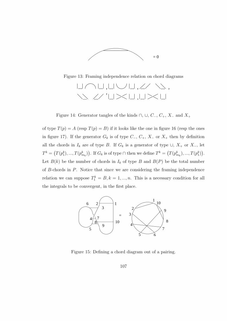
= 0
Figure 13: Framing independence relation on chord diagrams
, , ,,
,
... ... ... ... ... ...
..................
Figure 14: Generator tangles of the kinds ∩, ∪, C−, C+, X− and X+
of type T (p) = A (resp T (p) = B) if it looks like the one in figure 16 (resp the ones
in figure 17). If the generator Gk is of type C−, C+, X− or X+ then by definition
all the chords in Ik are of type B. If Gk is a generator of type ∪, X+ or X−, let
T k =(
T (pk1), ..., T (pkmk
))
. If Gk is of type ∩ then we define T k =(
T (pkmk), ..., T (pk1)
)
.
Let B(k) be the number of chords in Ik of type B and B(P ) be the total number
of B-chords in P . Notice that since we are considering the framing independence
relation we can suppose T k1 = B, k = 1, ..., n. This is a necessary condition for all
the integrals to be convergent, in the first place.
=
13
4
5
6
78
910
4
5
8
9
10
7
6
3
2
12
Figure 15: Defining a chord diagram out of a pairing.
107

... ...
Figure 16: A chord of type A
... ...
Figure 17: Chords of type B
Explicit calculations prove:
Lemma 54 8 Fix a knot K as before, there exists a C < +∞ such that for any
pairing P with m chords we have:
|Z(P,K)| ≤ Cm
n∏
k=1
1
B(k)!
n∏
k=1
∏
i∈1,...,mkT ki =A
1
#j ∈ 1, .., i : T kj = B . (67)
Proof. (sketch) Let T = (T1, .., Tn) be a sequence of A’s and B’s with T1 = B. Let
B(T ) be the number of elements of T equal to B, and let C(A) = 1 and C(B) = 1/2.
We have:
I(T ) =
∫
0<t1<...<tm<1
m∏
i=1
1
tC(T (Ai))i
dt1...dtm = 2m1
B(T )!
∏
i∈1,...,mTi=A
1
#j ∈ 1, ..., i : Tj = B . (68)
8See Theorem 69.
108

One proves this from the equality
∫
−∞<x1<x2<...<xn<0
e∑n
i=1 λixidx1...dxn =1
λ1(λ1 + λ2)...(λ1 + λ2 + ...+ λn), (69)
(easy to prove by induction if λ1, λ2, ..., λn > 0) by a continuity argument. Consider
the generators ∪ and ∩ to be made of semicircles of radius 1 and strings parallel
to z-axis. Unpacking equation (66) yields a product of n integrals, one for each Ik,
equal to, or bounded by, integrals like CmkI(T ), where C is fixed.
Let z ∈ C be a complex number, and let λz be the central character of the represen-
tation of sl(2,C) of highest weight 2z. We wish to give an estimate for |λz(φs(wP ))|,where s denotes the infinitesimal R-matrix in sl(2,C) coming from a quarter of the
Cartan-Killing form and wP is the chord diagrams made out of the pairing P . Even
though φs(w) does not make sense in A′, since φs does not satisfy the framing inde-
pendence relations, wP does define a chord diagram, thus an element of A, and in
particular it makes sense to consider φs(wP ).
Recall the recursive evaluation of the sl(2,C) weight system φs : A → U(sl(2,C))
in [CV], theorem 1 9. Let w be a chord diagram and let a be a chord of it, thus
a divides the circle supporting w into two semicircles. Define C(a, w) as the set of
chords of w that cross a. It has cardinality x(a, w). We define w(a) as the chord
diagram obtained from w by removing a. Let b and c be distinct chords in C(a, w),
they have endpoints ea, eb, fa, fb such that ea and eb (resp fa and fb) lie in the same
semicircle. Define wX(a, b, c) (resp w||(a, b, c)) as the chord diagrams obtained from
w through removing a,b and c and adding two new chords joining ea with fb and eb
9See Theorem 44.
109

with fa (resp ea with eb and fa with fb). Theorem 1 of [CV] tells us:
(λz φs)(w) = (λz φs)(⊖w(a)− 2x(a, w)(λz φs)(w(a))+∑
b,c∈C(a,w)b6=c
2(
(λz φs)(wX(a, b, c))− (λz φs)(w||(a, b, c)))
. (70)
Let w be a chord diagram with m chords having a set α(w) of chords that do not
cross each others (we do not suppose that this set is maximal). Pick up a chord
a0 ∈ α(w). Consider a diagram w′ appearing in the recursive evaluation (70). Then
α(w′) = α(w) \ a0 is a set of chords of w′ that do not intersect each others. In
addition we always have x(a, w′) ≤ x(a, w), ∀a ∈ α(w′). We need to use the fact
that the chords of α(w) do not cross each others to prove this. An obvious induction
based on equation (70) and this last fact tells you:
|(λz φs)|(w) ≤ Sz(m−#α(w))∏
a∈a(w)
(
|cz|+ 2x(a, w)2 + x(a, w))
(71)
≤ Sz(m−#α(w))C#α(w)z
∏
a∈a(w)(1 + x(a, w))2 . (72)
Here cz = (λz φs)(⊖) and Cz = max(|cz|, 2). In general, if i ∈ N, we define Sz(i) =
max|λz φs(x)|, x ∈ Wi where Wi is the set of chord diagrams with k chords. The
recursive evaluation tells you again that Sz(i) ≤∏i
j=1(|cz|+ 2j2 + j) ≤ Cjz(j + 1)!2.
Given this last estimates we prove:
Lemma 55 Let z ∈ C there exist a constant Cz < +∞ such that the following is
true: Let w be a chord diagrams with m chords having a set α(w) of chords that do
not cross each others. We have the estimate:
|(λz φs)|(w) < Cmz (k + 1)!2
∏
a∈a(w)(1 + x(a, w))2 , (73)
110

where k = m−#α(w). If in addition x(a, w) 6= 0, ∀a ∈ α(w) we can write this in a
more useful form for later, namely
|(λz φs)|(w) < (2Cmz )(k + 1)!2
∏
a∈a(w)(x(a, w))2 . (74)
Let K be an oriented knot and let P be a pairing with m chords. We want to apply
the lemma above to wP , the chord diagram made out of P . Each chord p of P gives
rise to a chord ap of wP . Two chords ap, ap′ with p and p′ chords of type A cannot
cross each others, therefore we define α(wP ) = ap : T (p) = A. If p is defined in
a generator G of K of type ∪ (resp. ∩), then x(ap, wP ) is the number of B-chords
defined in the same generator G staying bellow (resp. above) p, thus x(ap, wP )
can be supposed to be different of zero by the framing independence relation, since
T k1 = B. Combining lemmas 54 and 55, we conclude there exists a C < +∞ such
that:
|(λzφs)Z(P,K)wP | ≤ Cm (B(P )!)2∏n
k=1B(k)!
n∏
k=1
∏
i∈1,...,mkT ki =A
#j ∈ 1, .., i : T kj = B (75)
where C only depends on z and K. Notice B(P ) = B(1) + ...+B(n) is the number
of chords in P of type B.
An easy consequence of Stirling inequalities is the fact that given n ∈ N, there
exists a C < ∞ such that m! ≤ Cmm1!...mn!, where m1 + ... + mn = m, for any
m1, ..., mn ∈ N. Another consequence is the fact that there exists a C < +∞ such
that mm < Cmm!, ∀m ∈ N. Let K be a knot and P a pairing with m chords.
111

Putting everything together we prove
|(λz φs)(Z(P,K)wP )| ≤ CmB(P )B(P )B(P )A(P ) (76)
≤ Cm(A(P ) +B(P ))A(P )+B(P ) (77)
≤ Dmm!, (78)
for any pairing with m chords. Here A(P ) is the number of chords of P of type
A. Notice D < +∞ only depends on z and K. We know s = −t/4 thus ft(w) =
(−4)mφs(w), where m is the number of chords of w. therefore we can also find a
constant C < +∞ such that:
|(λz φt)(Z(P,K)wP )| ≤ Cmm!. (79)
We have now done the most difficult part of the proof of Theorem 34, even though
this last inequality is not quite enough yet. Let us go back to the definition of the
Kontsevich Integral. Let ∞ be a Morse knot equivalent to the unknot but with
4 critical points. Let N be the number of critical points of K. The unframed
Kontsevich integral of K is
Zu(K) =Z(K)
Z(∞)N/2. (80)
Let us define the framed version of the Kontsevich Integral. Recall we have a
coproduct in Afin defined by D(w) =∑
x⊂w x ⊗ (w \ x), whenever w is a chord
diagram. Here x is a chord diagram made out some chords of w and w \ x is the
complementary diagram. Recall Afin has a grading deg where the grading coefficient
of a chord diagram is its number of chords. Consider the map ψ : Afin → Afin such
that
ψ(w) =∑
x⊂w(−⊖)deg(x)(w \ x). (81)
112

for a chord diagram w. Thus ψ satisfies the 4T -relation. In fact ψ is a Hopf algebra
projection, see [Wi2] (this is not a trivial fact). The morphism ψ is zero on the ideal
generated by ⊖, thus ψ defines an algebra morphism A′fin → Afin. It extends to a
morphism ψ0 : A′ → A of the graded completions.
Definition 56 The Kontsevich Integral of K is
Z(K) = e⊖F (K)hψ0(Zu(K)) ∈ A, (82)
where F (K) is the framing coefficient of K.
This definition is equivalent to the standard one. See [Wi1] or [LM2] theorem 5.13.
Notice ψ(Z(∞))−1 = Z(O), which is the (framed) Kontsevich Integral of the zero
framed unknot. Let z ∈ C. Since (λz φt) is an algebra morphism, we have:
Jz(K)
2z + 1= (λz φt)Z(K) (83)
= (λz φs)(
e⊖F (K)h)
(λz φs)(
ψ0(Z(∞))−N/2)
(λz φt)(ψ0(Z(K))) (84)
= eczh(λz φt) (Zf (O))N/2 (λz φt)(ψ0(Z(K)) (85)
= eczh(
1
2z + 1
sinh((2z + 1)h/2)
sinh(h/2)
)N/2
(λz φt)(ψ0(Z(K)). (86)
Since the set G1[[h]] of power series of Gevrey type 1 forms an subalgebra of C[[h]],
the proof of theorem 34 will be finished if we prove that
(λz φt)(ψ0(Z(K)) =
∞∑
m=0
hm∑
pairings PP=zj ,z′j :Ikj→C,j=1,...,m
(λz φt)(ψ0(Z(P,K)wP ) (87)
is of Gevrey type 1. The estimate for |λz(φs)(w)| in 73 continues to hold if we
remove a chord from w, maintaining the right hand side of 73 fixed. Immediately
113
we have:
|(λz φs)|(ψ0(w)) ≤∑
x⊂w|(λz φs)(−⊖)|deg(x)|(λz φs)(w \ x)| (88)
≤ (2Cz)mCm
z (k + 1)!2∏
a∈a(w)(1 + x(a, w))2 . (89)
Recall that cz = (λz φs)(⊖) and Cz = max(|cz|, 1). Notice there are 2m splittings
w = x ∪ (w \ x) if w is a chord diagram with m chords. As before we prove.
Lemma 57 The estimate 79 continues to hold if we put (ψ0(Z(P,K)wP ) instead of
(Z(P,K)wP ).
We now prove (λz φt)(ψ0(Z(K)) ∈ G1[[h]]. Since we have proved Lemma 57, a
glance at equation 87 reduces the proof of this to estimating the number of pairings
P with m-chords, which is a simple exercise of counting. Let M = maxt∈R #((t ×C) ∩K). Consider pairings P with m chords, having mi chords in each interval Ii
for i = 1, ..., n, thus m1 + ...mn = m. There are at most (M(M − 1)/2)m pairings
like this. Recall the classical combinatorics problem which asks about the number
of ways we can put X indistinguishable objects into N distinguishable boxes. Its
solution is (N+X−1)!(N−1)!X!
. In our case we have exactly X = m objects (chords) and N = n
boxes (intervals Ik). Thus there are at most (M(M −1)/2)m (n+m)!(n−1)!m!
pairings P with
m chords. Given that n and M are constant, this last term grows exponentially
with respect to m. This finishes the proof of theorem 34.
114

6 On the Kontsevich Integral
The main aim of this Chapter is to describe the Kontsevich Integral in a way such
that we can prove Theorem 34
6.1 Definition of the Kontsevich Universal Knot Invariant
We freely use the notation of 1.1. We will work the C1 category, which permits us to
use the Kontsevich integral as the definition of the unframed Kontsevich Universal
knot invariant. A (oriented) knot K is an oriented C1 submanifold of R3 diffeomor-
phic with the oriented circle S1. Two knots K and K ′ are said to be isotopic if there
exists a C1 diffeomorphism f : R3 → R3 connected with the identity sending K to
K ′. A knot parametrisation is a C1 embedding γK : S1 → K ⊂ R3.
6.1.1 Framing independence relation in chord diagrams and the algebra
A′
Consider the equivalence relation on the space of chord diagrams shown on figure
18. It is called framing independence relation.
A chord c like in figure 18, such that there are no extreme points of any other chord
between its initial and end points, is called a isolated chord. Obviously, the sub
vector space 1T of Afin generated by the chord diagrams with isolated chords is an
ideal of Afin, in fact it is the ideal < ⊖ > generated by the chord diagram with only
one chord. Therefore A′fin = Afin/1T is an abelian algebra. It has an obvious grading
similar to the grading of A, where the grading coefficient of a chord diagram is given
its number of chords. Therefore A′, by definition the graded completion of A′fin, is
115
=0
Figure 18: Framing Independence Relation
also an abelian algebra. This algebra is the target space for both the Kontsevich
Integral and Unframed Kontsevich Universal Knot Invariant.
6.1.2 Unframed Kontsevich Universal Knot Invariant
As described for example in [BN] there exists a map K Zu−→ A′, which is called
the Unframed Kontsevich Universal Knot Invariant. Let us describe how it is con-
structed out of the Kontsevich Integral. Another good reference for the description
of the Kontsevich Integral is [CD], which we follow closely. To begin with we recall
the definition of Morse functions. These are functions f : S1 → R, such that:
1. f is C1.
2. Each critical point of f is either a local maximum or a local minimum.
3. f attains different values at each extreme point.
4. The set of critical points of f is finite.
Consider a knot K and a parametrisation γ : S1 → R3 ∼= R × C of it. Let t(s) be
the projection of γ(s) in the first variable. Apart from possibly applying an isotopy
of R3, we can suppose t(s) is a Morse function. Let t0, ..., tn be the set of critical
points of t. Suppose t0 < ti < ... < tn, and define Ik = (tk−1, tk), k = 1, ..., n. Given
116
a positive integer m, define:
Ik,m = (x1, ..., xm) ∈ Rm : tk−1 < x1 < ... < xm < tk, k = 1, ..., n.
We consider also Ik,0 = 0, k = 1, ..., n. Therefore the volume of Ik,m is 1m!(tk −
tk−1)m. Suppose m > 1 is a integer. For any finite sequence m = (m1, ..., mn) ∈ Nn
0 ,
define
Im = I1,m1 × ...× In,mn .
Let k ∈ 1, ..., n. The intersection Kt = (t × C) ∩ K has a constant number
of points in Ik. See figure 19. Obviously all the sets Kt, t ∈ Ik can be identified
with a finite set S(k) in such a way the obvious map K ∩ (Ik × C) → S(k) is
continuous. Let p ∈ S(k), we can define uniquely a map zp : Ik → C such that
(t, zp(t)) = p, ∀t ∈ Ik, by the implicit function theorem zp is C1. It can be extended
obviously to a continuous function zp : [tk−1, tk] → C.
Denote by S(2)(k) the set of subsets of S(k) with 2 elements. We call them chords.
There exists a subset D+(k) ⊂ S(2)(k), the set of elements p, q ∈ S(2)(k) for which
(tk, zp(tk)), (tk, zq(tk)) are both local maxima. The set D−(k) is defined analogously
as the set p, q ∈ S(2)(k) for each (tk−1, zp(tk−1)), (tk, zq(tk)) are both local minima.
Notice that each set D+(k), D−(k) has cardinality at most one by the condition 4
of the definition of Morse functions.
Let us be given an integer m > 0 and a k ∈ 1, ..., n. We associate to them a
finite set Pkm. An element of Pk
m is a map P k : 1, ..., m → S(2)(k) of the form
i 7→ pk(i), p′k(i), equivalently a map i → zki(t), z′ki(t), t ∈ Ik. The map P k
is called a pairing and each zk, z′k a chord of it. We put the condition that
pk(m), p′k(m) /∈ D+(k) and pk(1), p′k(1) /∈ D−(k).
117

t
t
t
t
0
1
2
3
x
y
t
z’(t)z(t)
Non admissible pairing
Admissible pairing
1
I 3
I 2
I
Figure 19: Admissible and Non Admissible pairings
Definition 58 An element of P k ∈ Pkm is called a k-admissible pairing. See figure
19
Proposition 59 Given an admissible pairing P k = i 7→ zki(t), z′ki(t) ∈ Pkm,
the following integral is absolutely convergent:
Z(k,m, P k) =
∫
Ik,m
m∧
i=1
dzki (xi)− dz′ki (xi)
zki (xi)− z′ki (xi). (90)
This will the basis for the definition of the Kontsevich integral.
Definition 60 Suppose we are given a sequence m = (m1, ..., mn) ∈ N0n, an m-
pairing P (admissible) is a map
P ∈ 1, ..., n → P k ∈n⊔
k=1
Pkmk,
118

I 1
I
I 2
I
I
3
4
5
Figure 20: A (0, 3, 2, 3, 0)-pairing
with P k ∈ Pkmk, k = 1, ...n a k admissible pairing. Let Pm designate the set of all
m-pairings. Any pairing P defines a chord diagram ωP in the obvious way. Let for
any P ∈ Pm:
Z(m,P ) =
n∏
k=1
Z(k,mk, P (k)).
The reader is advised to look at figure 20. Notice there are no pairings with m1 or
m5 not equal to zero, for then the pairings P 0 and P 5 would not be admissible.
One more simple ingredient is necessary to define the Kontsevich universal knot
invariant. Let us be given a pairing P , then #P is defined as the number of zki or
119
z′ki on which t(s) is decreasing.
Let m = (m0, ..., mn) ∈ Nn0 , we put |m| = m0 + ... +mm.
Definition 61 Consider a C∞ parametrisation γ : S1 → R × C such that the
projection t(s) in the first variable is a Morse function with n + 1 critical points.
Define for every integer m > 1:
Z(γ,m) =∑
m∈N0n:|m|=m
P∈Pm
(−1)#PZ(m,P )wP .
Define also Z(γ, 0) = 1,Z(γ, 1) = 0. The Kontsevich integral is by definition:
Z(γ) =∑
m∈N0
1
(2πi)mZ(γ,m) ∈ A′.
Consider a parametrisation γ∞ of the unknot such that t(s) is a Morse function
having 4 critical points. The next two results are proved for example in [BN]
Theorem 62 The series Z(γ) does not depend on the chosen parametrisation γ∞
yielding the unknot as long as t(s) is a Morse function which have exactly 4 critical
points. Call the series obtained Z(∞).
Notice that Z(∞) is invertible in A′ for its first term is 1.
Theorem 63 Let us be given a knot K, with a parametrisation γK of it such that
t(s) is a Morse function with n + 1 critical points. Notice n + 1 is a positive even
number. Define
Zu(K) =Z(γK)
Z(∞)n+12
120

Then Zu(K) does not depend on the isotopy class of of K, as long as t(s) is a
Morse function, which we can suppose apart from isotopy. Therefore Zu(K) is a
knot invariant. Call it the unframed Kontsevich Universal Knot invariant.
6.1.3 Framed Kontsevich Universal Knot Invariant
We now extend the Kontsevich Universal Knot Invariant for framed knots. This
extension is referred to usually as the framed Kontsevich Universal Knot Invariant.
Recall that a framed knot K is an embedding of the stripe S1× [−1, 1] into R3 with
the obvious notion of isotopy class. Any framed knot defines an isotopy class of
knots in the obvious way. The framing coefficient F (K) of a framed knot K is the
linking number of K × −1 and K × 1.
Recall that the algebra A′ is defined as the graded completion of A′fin = Afin/ < ⊖ >,
where < ⊖ > is the ideal ofAfin generated by the chord diagram with only one chord.
Both Afin and A′fin have gradings for which the grading coefficient deg(ω) of a chord
diagram is given by its number of chords. Consider the map φ : Afin ⊗Afin → Afin
such that if ω1 and w2 are chord diagrams we have φ(ω1 ⊗ ω2) = (−⊖)deg(ω1)w2.
Define ψ : Afin → Afin as ψ = φ ∆. Then actually ψ2 = ψ and ψ is a Hopf
algebra morphism (this is a non trivial fact). Its kernel is contained in < ⊖ >, thus
ψ descends to a map ψ′ : A′fin → Afin, which can be extended to all A′ since ψ′
preserves gradings. See [Wi2] for more details. Let p : A′ → A be the projection.
Given that ψ(⊖) = 0 it follows
ψ′ p = ψ. (91)
121

Definition 64 The (framed) Kontsevich Universal Knot Invariant is:
Zf (K) = Z(K) = ψ′(Zu(K)) exp(F (K)⊖),
where the convergence of the series defining e(F (K)⊖) is understood in the graded alge-
bra sense. Here Zu(K) denotes the unframed Kontsevich Universal Knot Invariant.
Recall F(K) is the framing coefficient of the knot K.
Recall the Kontsevich Universal Knot Invariant satisfies all the properties stated in
theorem 1.
This is a slightly ad-hoc definition of the framed Kontsevich Universal knot invariant.
However it is equivalent to the standard one. This was pointed out in [Wi1]. The
proof of this fact appears in [LM2]( theorem 5.13). Let us give an idea of how this
result can be proved. I only know one place where this result is proved, namely
[LM2].
Proof. (sketch) We can either define the Framed Kontsevich Universal Knot
Invariant Z ′ out of the Drinfeld Associator as in [LM2]; or by regularising the
integral (90) for non admissibe pairings through considering
limε→0,ε>0
Z(Ke) exp
(− ln(ε)
2πi⊖)
,
at each minimal point, say, where Kε is the tangle obtained from the knot K by
removing the points in the two strands making the minimal point which are at
smaller distance than ε. We do analogously for maximal points considering
limε→0,ε>0
Z(Ke) exp
(
ln(ε)
2πi⊖)
.
At the end we obviosly consider the limit for all maximal and minimal points simul-
taneously. See [LM2] for more details. Notice that both definitions of the Framed
122

Kontsevich Universal Knot invariant yield isotopy invariants of blackboard framed
knots. This is because we are implicitly choosing determination of the logarithm at
each extreme point. Call these two definitions ZD and ZR. It is well known that
they are equivalent, that is Z ′ = ZR = ZD, see [LM2] or [AF]. Let us prove both
are equal to Z, as in Definition 64.
Consider the algebra projection p : A → A′. From the second definition of Z,
the one involving the regularisation of the Kontsevich Integral, it is immediate that
p Z ′ = Zu. Therefore ψ′ Zu = ψ′ p Z ′ = ψ(Z), by (91). Therefore, we
only need to find the relation between ψ Z ′ and Z ′. It is now better to consider
Z ′ = ZD, the definition of the Kontsevich Universal Knot Invariant involving the
Drinfeld associator as in [LM1]. Let φ(A,B) be the Drinfeld associator, constructed
from the monodromy of the Kniznick-Zamolodchikov equations. See [D1], [D2],
[K] or [LM3]. It is an element of the algebra C[[A,B]] of power series in two non
commuting variables A and B. We now follow [LM3] and [K]. Consider the algebra
C[[A,B]]][α, β] of polynomials in α, β with coefficients in C[[A,B]] (we suppose α
and β commute with all other variables). A beautiful identity satisfied by φ(A,B)
is
φ(A− α,B − β) = φ(A,B), in C[[A,B]][α, β]
Therefore if c commutes with all variables we have
φ(A− c, B − c) = φ(A,B), in C[[A,B]][c]] (92)
see [LM1] page 63 or [K] page 469. A proof of this fact is not that difficult, but
involves going through all the definition of φ(A,B). Equation 92 is more or less
obvious from the fact φ(A,B) is an exponential of a series of commutators in A and
123

B.
Let K be a framed knot. It is better now to see ψ : A → A as a map such that if ω
is a chord then ψ(ω) = w− b1/2− b2/2, where b1 (resp b2) is a chord connecting two
points in a neighbourhood of one (resp other) extreme point of w; and analogously
for more complicated chord diagrams. The advantage is that it makes also sense to
consider ψ(ω) where ω is a chord diagram supported on a tangle. The evaluation
of ZD(K) is made out of terms like φ(Hi,j, Hi,j), where Hi,j means connecting the
ith and jth strands of K by a chord perpendicular to the t axis. We also have terms
like exp(Hi,j) at each crossing point. Consider applying ψ to ZD(K). The terms
involving φ(Hi,j, Hj,k) are easy to deal with: by 92 they remain unaltered since ⊖commutes with any chord diagram. Since ψ is an algebra morphism, the evaluation
of exp(Hi,j) will change as exp(Hi,j − b1/2 − b2/2), which, since ⊖ commute with
all variables, is exp(Hi,j) exp(−⊖). This is the reason why the factor exp(F (K)) in
Definition 64 appears. We thus need to have Z = Z ′. See [LM2] for details.
6.1.4 Some bounds for the coefficients of Kontsevich Universal Knot
Invariant
We now estimate the modulus of the coefficients of the Kontsevich integral for knots.
This will be used in the proof of theorem 34. We freely use the notation of 6.1.2.
This will be a rather long section, not very difficult, but with a large amount of
notation being introduced.
Let K be a knot and let γ : S1 → R × C be a Morse parametrisation of it. To
calculate Z(γ), we need to know the critical points t0 < t1 < ... < tn of t(s) of γK .
If Ik = [tk+1, tk] then I1 ∪ ... ∪ In is a splitting [t0, tn] = γK(S1) such that no critical
124

point of γK is in the interior of any interval Ik. However to calculate Z(γ), we can
use any splitting τ0 = c0 < c1 < .... < cN = tn of the interval [t0, tn] as long as the
set of critical points of t(s) is contained in c0, ..., cN. See [BN], 4.3.2. This is a
consequence of the fact that away from extreme points the Kontsevich Integral is
expressed as the holonomy of the formal Kniznick-Zamolodchikov connection. See
[BN]
Let K be an oriented knot, it can be seen as the closure of some braid b ∈ B(n) for
some n ∈ N. Here B(n) is the braid group with n-strands. A parametrisation γK of
K will have therefore 2n critical points. Fix once for all a braid b ∈ B(n), for some
n ∈ N such that its closure is K. We want to calculate Z(K) out of the closure of
b, thus for definiteness we explicitely construct such a closure. The braid b consists
of n oriented downwards strands connecting the points (1, 0), (1, 1), ..., (1, n− 1) to
(−1, 0), (−1, 1)..., (−1, n). Strands which can be supposed contained in [−1, 1]×z ∈C : |z| < n. Consider an explicit construction of a closure of b as in figure 21. That
is:
Consider n straight lines oriented upwards connecting
• (n+ 1, 1) to (n+ 1,−1)
• (n+ 2, 1 + 1) to (n+ 2,−(1 + 1))
• (n+ 3, 1 + 1 + 2) to (n+ 3,−(1 + 1 + 2))
• (n+ 4, 1 + 1 + 2 + 3) to (n+ 4,−(1 + 1 + 2 + 3))
• and so on until
• (n+ n, 1 + 1 + 2 + 3 + ...+ n− 1) to (n + n,−(1 + 1 + 2 + 3 + ...+ n− 1))
125

b
I
I
I
I
I
I
I
2
0
−2
−3
−1
1
3
Figure 21: Closure of a braid
126

Also, connect the points
• (n− 1, 1) to (n− 1, 1)
• (n− 2, 1) to (n− 2, 1 + 1)
• (n− 3, 1) to (n− 3, 1 + 1 + 2)
• (n− 4, 1) to (n− 4, 1 + 1 + 2 + 3)
• and so on until
• (n− n, 1) to (n− n, 1 + 1 + 2 + 3 + ...+ n− 1)
By oriented downwards straight lines.
Similarly, use oriented downwards straight lines, and connect the points
• (n− 1,−1) to (n− 1,−1)
• (n− 2,−1) to (n− 2,−(1 + 1))
• (n− 3,−1) to (n− 3,−(1 + 1 + 2))
• (n− 4,−1) to (n− 4,−(1 + 1 + 2 + 3))
• and so on until
• (n− n,−1) to (n− n,−(1 + 1 + 2 + 3 + ... + n− 1))
Now, use semicircles of radius k oriented counterclockwise, chosen so that the closure
of the braid has a C1 parametrisation, to connect the points
127
• (n+ 1, 1) to (n− 1, 1)
• (n+ 2, 1 + 1) to (n− 2, 1 + 1)
• (n+ 3, 1 + 1 + 2) to (n− 3, 1 + 1 + 2)
• (n+ 4, 1 + 1 + 2 + 3) to (n− 4, 1 + 1 + 2 + 3)
• and so on until
• (n+ n, 1 + 1 + 2 + 3 + ...+ n− 1) to (n− n, 1 + 1 + 2 + 3 + ...+ n− 1)
And, similarly
• (n+ 1,−1) to (n− 1,−1)
• (n+ 2,−(1 + 1)) to (n− 2,−(1 + 1))
• (n+ 3,−(1 + 1 + 2)) to (n− 3, (1 + 1 + 2))
• (n+ 4,−(1 + 1 + 2 + 3)) to (n− 4,−(1 + 1 + 2 + 3))
• and so on until
• (n+ n,−(1 + 1+ 2+ 3+ ...+ n− 1)) to (n− n,−(1 + 1+ 2+ 3+ ...+ n− 1))
The reader is strongly advised to look at figure 21. Let γ : S1 → R × C be the
parametrisation of K just constructed. Define r0 = 1, r1 = 1 + 1, r3 = 1 + 1 +
2, ..., rn = 1 + 1 + 2 + 3 + ... + n. Split γ(S1) = [−rn, rn] as [−rn,−rn−1] ∪ ... ∪[−r2,−r1]∪ [−r1, r1]∪ [r1, r2]∪ ...∪ [rn−1, rn] = I−n∪I−n−1∪ ...∪I−1∪I0∪I1∪ ...∪In
128

Figure 22: A chord of type A
Figure 23: Chords of type B1
Definition 65 (Chord Type) Let P k ∈ Pkm with k ∈ −n, ...,−1 ∪ 1, ..., n,
be a k-admissible pairing with m chords, in other words a map i 7→ pi = zi, z′i,where i ∈ 1, ..., m and z, z′ : Ik → C. We divide the chords pi = zi, z′i into
two different types: A chord is said to be of type A, say, if it looks like the chord in
figure 22. We say it is of type B otherwise. Chords of type B can appear on types
B1 and B2 shown in figures 23 and 24. If k = 0 then by definition we say that all
the chords are of type B2. If Pk is a k-admissible pairing then A(P k) (resp B(P k))
is the number of chords of P of type A (resp B), thus A(P k) + B(P k) = m, which
is the number of chords of P k. For a chord p, let T (p) denote its type.
Definition 66 (Type Sequences) Let b be a braid with n strands whose closure
is a knot and k ≤ 0. Let also P k ∈ Pkm be a k-admissible pairing with m-chords.
129

Figure 24: chords of type B2
The type sequence of P k is by definition
T (P k) = (T (p1), T (p2), ..., T (Pm)).
If k > 0 then by definition
T (P k) = (T (pm), ..., T (p2), T (p1)).
Notice that since the pairings are admissible, the first letter of the type sequences
is always B. Let m = (m−n, ..., m0, ..., mm) be a sequence in N2n+10 . Let also P ∈
Pm be a m pairing, thus for each k ∈ −n..., n, we have type sequences T (P k)
characterising the pairing P k ∈ Pkmk
. Let B(P ) and A(P ) be the number of chords
of P of type B and A, respectively, thus A(P ) = A(P−n)+ ...+A(P n), and similarly
for B(P )
The reader is advised to look at figures 25 and 26.
Consider a pairing in Pkm with k 6= n. Due to the way we defined the closure of the
braid b, it is very easy to determine the functions zp : In → C. Only two of them will
be non constant. If k is positive, then they are the obvious shifting of ±√k2 − t2,
and analogously if k is negative.
130

Figure 25: An example with T (P ) = (B,B,A,B,B,B,B,A,B)
Figure 26: An example with T (P ) = (B,B,B,B,A,A,B,B,A)
Lemma 67 Let us be given a k ∈ −n, ...,−1∪1, ..., n, m ∈ N and a k-admissible
pairing P k = i 7→ zki (t), z′ki (t) ∈ Pkm. We have the estimate
|Z(k,m, P k)| =∣
∣
∣
∣
∣
∫
Ik,m
m∧
i=1
dzki (xi)− dz′ki (xi)
zki (xi)− z′ki (xi)
∣
∣
∣
∣
∣
≤ k−B(P k)
B(P k)!
∏
i∈1,...,mT (P k)(i)=A
1
#j ∈ 1, ..., i : T (P k)(j) = B ,
where T (P k) = (T (P k)(1), ..., T (P k)(m)) is the type sequence of P k. Here # denotes
the cardinal of a set.
Proof. We make the proof for k ∈ 1, ..., n, the other proof will be analogous.
Obviously:
|Z(k,m, P k)| =∫
0<x1<x2<...<xm<k
f1(x1)...fm(xm)dx1...dxm.
131

Here fi(t) can be a function of the kinds: B(l), l > k, where
B(l)(t) =
∣
∣
∣
∣
∣
ddt
(
l ±√k2 − t2
)
l ±√k2 − t2
∣
∣
∣
∣
∣
=
∣
∣
∣
∣
1
l ±√k2 − t2
t√k2 − t2
∣
∣
∣
∣
<t√
k2 − t2, l > k,
if the associated chord P k(i) is of type B1; A(t), where
A(t) =t
k2 − t2=
∣
∣
∣
∣
∣
ddt
√k2 − t2√k2 − t2
∣
∣
∣
∣
∣
,
if the associated chord P k(i) is of type A; or the null function if the associated
chord P k(i) is of type B2. Since we are considering admissible pairings, we also have
fm 6= A. This is a crucial condition for the integral to be convergent in the first
place. Let ai = 1/2 if the ith chord is of type B and 1 if the ith chord is of type A,
thus am = 1/2. We have:
|Z(k,m, P k)| ≤∫ k
0
dx1x1
(k2 − x21)a1
∫ k
x1
dx2x2
(k2 − x22)a2
∫ k
x2
dx3x3
(k2 − x23)a3
∫ k
x3
dx4...
∫ k
xm−1
dxmxm
√
k2 − x2m= I.
Consider the coordinate change xi = kx′i, we obtain:
I = k−B(P k)
∫ 1
0
dx′1x1
(1− x′12)a1
∫ 1
x′1
dx′2x′2
(1− x′22)a2
∫ 1
x′2
dx′3x′3
(1− x′23)a3
∫ 1
x′3
dx4...
∫ 1
x′m−1
dx′mx′m
√
1− x′2m.
Thus if we put x′i =√1− yi, i = 1, ..., m yields:
I =k−B(P k)
2m
∫ 1
0
dy11
ya11
∫ y1
0
dy21
ya22
∫ y2
0
dy31
ya33
∫ y3
0
dy4...
∫ ym−1
0
dym1√ym
=k−B(P k)
2m
∫ 1
0
dym1√ym
∫ 1
ym
dym−11
yam−1
m−1
∫ 1
ym−1
dym−21
yam−2
m−2
∫ 1
ym−2
dym−3...
∫ 1
y2
dy11
y1a1
132
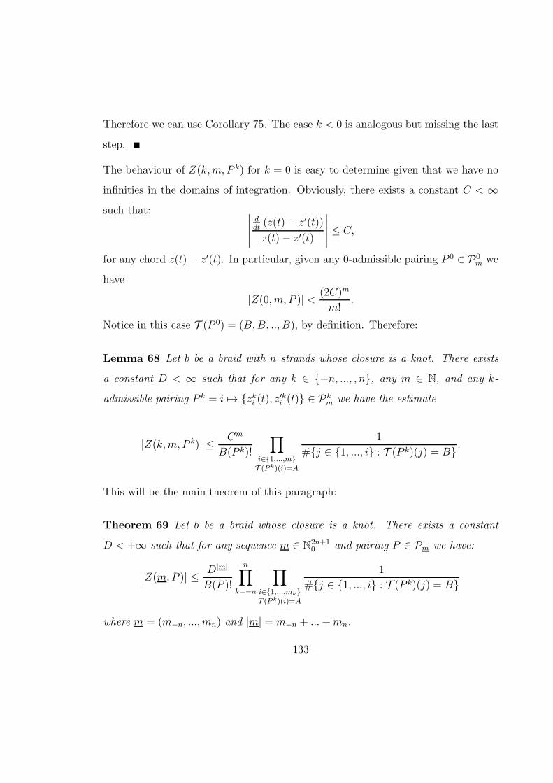
Therefore we can use Corollary 75. The case k < 0 is analogous but missing the last
step.
The behaviour of Z(k,m, P k) for k = 0 is easy to determine given that we have no
infinities in the domains of integration. Obviously, there exists a constant C < ∞such that:
∣
∣
∣
∣
∣
ddt(z(t)− z′(t))
z(t)− z′(t)
∣
∣
∣
∣
∣
≤ C,
for any chord z(t)− z′(t). In particular, given any 0-admissible pairing P 0 ∈ P0m we
have
|Z(0, m, P )| < (2C)m
m!.
Notice in this case T (P 0) = (B,B, .., B), by definition. Therefore:
Lemma 68 Let b be a braid with n strands whose closure is a knot. There exists
a constant D < ∞ such that for any k ∈ −n, ..., , n, any m ∈ N, and any k-
admissible pairing P k = i 7→ zki (t), z′ki (t) ∈ Pkm we have the estimate
|Z(k,m, P k)| ≤ Cm
B(P k)!
∏
i∈1,...,mT (P k)(i)=A
1
#j ∈ 1, ..., i : T (P k)(j) = B .
This will be the main theorem of this paragraph:
Theorem 69 Let b be a braid whose closure is a knot. There exists a constant
D < +∞ such that for any sequence m ∈ N2n+10 and pairing P ∈ Pm we have:
|Z(m,P )| ≤ D|m|
B(P )!
n∏
k=−n
∏
i∈1,...,mkT (P k)(i)=A
1
#j ∈ 1, ..., i : T (P k)(j) = B
where m = (m−n, ..., mn) and |m| = m−n + ...+mn.
133

Proof. This follows from Proposition 68 and Lemma 70.
6.1.5 Some calculations
We prove the lemmas that we have just used used, as well as some results that will
be useful later. First of all recall Stirling’s inequality for n!:
√2πm
mm
eme
112m+1 < n! <
√2πm
mm
eme
112m , m = 1, 2, ... (93)
It will be used quite frequently later. Immediately to prove:
Lemma 70 Let n be an integer. There exists a C > 0 such that for all sequences
m = (m1, ..., mn) ∈ Nn0 we have
|m|!(m1!)(m2!)...(mn!)
≤ C |m|,
where as usual |m| = m1 +m2 + ... +mn.
Proof. Let m = |m|. Suppose mi 6= 0, ∀i. The Stirling inequalities prove:
m!
(m1!)(m2!)...(mn!)<
mm
(mm11 )(mm2
2 )...(mmnn )
√2π
√m√
2πn√m1...mn
e1
12m1+1 e1
12m2+1 ...e1
12mn+1
e1
12m
.
Therefore for any m ∈ Nn:
m!
(m1!)(m2!)...(mn!)<
mm
(mm11 )(mm2
2 )...(mmnn )
√2π
√m√
2πnen.
We can thus choose a D > 0 such that:
m!
(m1!)(m2!)...(mn!)<
mm
(mm11 )(mm2
2 )...(mmnn )
Dm,
134
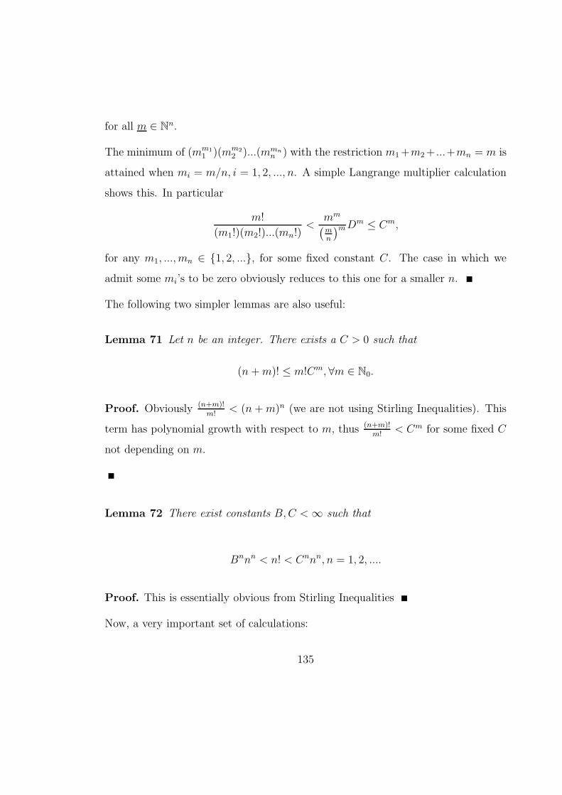
for all m ∈ Nn.
The minimum of (mm11 )(mm2
2 )...(mmnn ) with the restriction m1+m2+ ...+mn = m is
attained when mi = m/n, i = 1, 2, ..., n. A simple Langrange multiplier calculation
shows this. In particular
m!
(m1!)(m2!)...(mn!)<
mm
(
mn
)mDm ≤ Cm,
for any m1, ..., mn ∈ 1, 2, ..., for some fixed constant C. The case in which we
admit some mi’s to be zero obviously reduces to this one for a smaller n.
The following two simpler lemmas are also useful:
Lemma 71 Let n be an integer. There exists a C > 0 such that
(n +m)! ≤ m!Cm, ∀m ∈ N0.
Proof. Obviously (n+m)!m!
< (n +m)n (we are not using Stirling Inequalities). This
term has polynomial growth with respect to m, thus (n+m)!m!
< Cm for some fixed C
not depending on m.
Lemma 72 There exist constants B,C <∞ such that
Bnnn < n! < Cnnn, n = 1, 2, ....
Proof. This is essentially obvious from Stirling Inequalities
Now, a very important set of calculations:
135
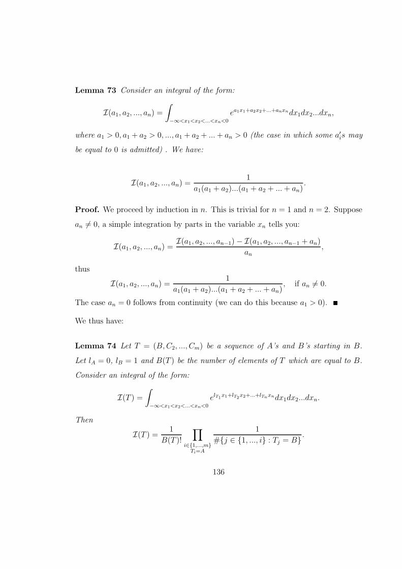
Lemma 73 Consider an integral of the form:
I(a1, a2, ..., an) =∫
−∞<x1<x2<...<xn<0
ea1x1+a2x2+...+anxndx1dx2...dxn,
where a1 > 0, a1 + a2 > 0, ..., a1 + a2 + ...+ an > 0 (the case in which some a′is may
be equal to 0 is admitted) . We have:
I(a1, a2, ..., an) =1
a1(a1 + a2)...(a1 + a2 + ...+ an).
Proof. We proceed by induction in n. This is trivial for n = 1 and n = 2. Suppose
an 6= 0, a simple integration by parts in the variable xn tells you:
I(a1, a2, ..., an) =I(a1, a2, ..., an−1)− I(a1, a2, ..., an−1 + an)
an,
thus
I(a1, a2, ..., an) =1
a1(a1 + a2)...(a1 + a2 + ... + an), if an 6= 0.
The case an = 0 follows from continuity (we can do this because a1 > 0).
We thus have:
Lemma 74 Let T = (B,C2, ..., Cm) be a sequence of A’s and B’s starting in B.
Let lA = 0, lB = 1 and B(T ) be the number of elements of T which are equal to B.
Consider an integral of the form:
I(T ) =∫
−∞<x1<x2<...<xn<0
elT1x1+lT2x2+...+lTnxndx1dx2...dxn.
Then
I(T ) = 1
B(T )!
∏
i∈1,...,mTi=A
1
#j ∈ 1, ..., i : Tj = B .
136
Therefore:
Corollary 75 Let T = (B, ...) be a sequence of A’s and B’s of length m starting in
the letter B. Let B(T ) be the number of B’s in it. Let ci = 1/2 if Ti = B and ci = 1
if Ti = A, for i = 1, ..., m. Then
I(T ) =
∫
0<x1<...<xn<1
n∏
i=1
1
xciidx1...dxm = 2m
1
B(T )!
∏
i∈1,...,mTi=A
1
#j ∈ 1, ..., i : Tj = B .
Proof. We just need to consider the change of variables xi = exp(2ti), i = 1, ..., m
and apply the previous lemma.
6.2 Proof of Theorem 34
Consider the Lie algebra sl(2,C) with its usual Cartan decomposition. The elements
H,E, F defined in 1.4.6 are a basis of it. The infinitesimal R-matrix coming from
minus the Cartan-Killing form in sl(2,C) expresses as
t = −1
4
(
E ⊗ F + F ⊗E +H ⊗H
2
)
.
Let z be a complex number, the highest weight representation of maximal weight 2z
is the representation ρzof spin z defined in 1.4.6. For the case z /∈ 1
2N0, it is defined in
the infinite dimensional space Vz
which has a basis of the form v2z, v2z−1, v2z−2, ....The action of H,E and F is:
Hvk = (k − z)vk; k = 2z, 2z − 1, ...,
137
Evk = (2z − k)vk+1; k = 2z, 2z − 1, ...,
F vk = kvk−1; k = 2z, 2z − 1, ....
If z ∈ 12N0 the definition is analogous but now the representation is in the space
v2z, ..., v0.
6.2.1 Prior estimate for matrix elements
Let λz : C(U(sl(2,C))) → C be the central character of ρz. Given a chord diagram w
with m chords, we wish to give a rough estimate for |λz(φt(w))|. Consider the innerproduct <,> on V
z
which has an orthonormal basis given by v2z, v2z−1, v2z−2, ....Obviously λz(φt(w)) =< v2z, φt(w)v2z >. Thus
λz(φt(w)) =
3m∑
i=1
⟨
v2z, Ai1A
i2...A
i2mv2z
⟩
,
where each Aik can be E2, F2or H
2√2. The term ”3m” comes from the fact the infinites-
imal R-matrix t is a sum of 3 terms. From this formula it is trivial to conclude that
z → λz(φt(w)) is polynomial in z of degree at most 2m, avoiding a proof using the
general theory on central characters and highest weight representations. Also
|λz(φt(w))| ≤3m∑
i=1
∣
∣
⟨
v2z, Ai1A
i2...A
i2nv2z
⟩∣
∣ .
Thus from the general expression of the spin z representations it follows that given
any z ∈ C, there exists a D > 0 such that for any chord diagram with m chords we
have:
|λz(φt(w))| ≤ DmΓ(|2z|+m+ 1)2.
Applying Lemma 71 we conclude.
138

Lemma 76 Let z be a complex number. There exists a constant C > 0 such that
for any chord diagram with m chords we have:
|λz(φt(w))| ≤ Cm(m!)2.
6.2.2 Refined estimate for matrix elements
The estimate we have just obtained for λz(φt(w)) is not good enough for our pur-
poses, namely to prove Theorem 34. However Theorem 44 in 5.2 (that is theorem 1
of [CV]), permits us to refine this estimate, depending on the kind of chord diagram
we have . We freely use the notation of 5.2, and frequently use the normalisation
s for the infinitesimal R-matrix of sl(2,C). Obviously, Lemma 76 is true if we use
φs instead of φt. This is going to be a long section with a large amount of notation
and nomenclature being introduced.
Definition 77 Let z be a complex number. Define cz = λz(φs(⊖)), here ⊖ is the
chord diagram with just one chord. It is the action of the rescaled Casimir operator
in the representation ρzof spin z.
Definition 78 (Crossing Number) Let ω be a chord diagram, and a be a chord
of it. The crossing number ×(a, ω) of a in ω is the number of chords of ω that cross
the chord a.
The following definition is the obvious counterpart of Definition 65. The reader is
advised to look at it again.
Definition 79 (Normal Chord Diagrams) Let ω be a chord diagram with m
chords. Suppose there are some chords a1, ..., an of ω which do not intersect each
139

α chords
chordsβ
Figure 27: A normal chord diagram showing α-chords and β-chords
others, call them α-chords. For each m ∈ 1...n, let bm1 , ..., bmkm
be the chords of ω
crossing am. Call these chords β1-chords. Notice that by definition km is the crossing
number of am in ω. We will have in addition a set of chords completing the chord
diagram, called β2-chords. Therefore β2-chords do not cross α-chords. A β-chord
is by definition either a β1-chord or a β2-chord. A chord diagram with an indexing
of chords like this is called normal. Obviously this definition depends on the way
we specify the α, β1 and β2-chords, since any α-chord can be called a β-chord. See
figure 27.
We have
Lemma 80 Consider applying Theorem 44 to a normal chord diagram ω and an
α-chord am ∈ a1, .., an of it. All the chord diagram ω(am), ω||(am, i, j); 1 ≤ i <
j ≤ km and ωX(am, i, j); 1 ≤ i < j ≤ km are normal with the same number of β
chords, with the set of α-chords losing the chord αm. Moreover the crossing number
140
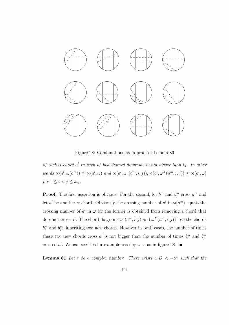
Figure 28: Combinations as in proof of Lemma 80
of each α-chord al in each of just defined diagrams is not bigger than kl. In other
words ×(al, ω(am)) ≤ ×(al, ω) and ×(al, ω||(am, i, j)),×(al, ωX(am, i, j)) ≤ ×(al, ω)
for 1 ≤ i < j ≤ km.
Proof. The first assertion is obvious. For the second, let bmi and bmj cross am and
let al be another α-chord. Obviously the crossing number of al in ω(am) equals the
crossing number of al in ω for the former is obtained from removing a chord that
does not cross αl. The chord diagrams ω||(am, i, j) and ωX(am, i, j)) lose the chords
bmi and bmj , inheriting two new chords. However in both cases, the number of times
these two new chords cross al is not bigger than the number of times bmi and bmj
crossed al. We can see this for example case by case as in figure 28.
Lemma 81 Let z be a complex number. There exists a D < +∞ such that the
141
following is true:
Let ω be a normal chord diagram with a set a1, ..., an of α-chords, where al has
crossing number kl. Let m be the number of chords of ω and mβ be the number of β
chords. We have
|(λz φs)(ω)| < Dm(mβ !)2
n∏
l=1
(2k2l + kl + |cz|).
Proof. We proceed by induction on mα, which is the number of α-chords. Choose
C as in Lemma 76 and let D = max(C, 1), thus the assertion is trivial for mα = 0.
Let ω be a normal chord diagram with a set α1, ..., αn of α-chords. By Theorem
44 we have
|(λz φs)(ω)| =∣
∣
∣
∣
∣
(λz φs)(
(⊖− 2kn)ω(an) + 2
∑
1≤i<j≤kn
(
ω||(an, i, j)− ωX(an, i, j))
)∣
∣
∣
∣
∣
≤ |(λz φs)(⊖)||(λz φs)(ω(an))|+ 2kn|(λz φs)(ω(an))|
+ 2∑
1≤i<j≤kn
(∣
∣(λz φs)(
ω||(an, i, j))∣
∣+∣
∣(λz φs)(
ωX(an, i, j))∣
∣
)
= |cz||(λz φs)(w(an))|+2k2n+kn∑
q=1
|(λz φs)(ωq)|,
where, as consequence of Lemma 80, for any q ∈ 1, ..., k2n + kn, the diagram ωq is
a normal chord diagram with m − 1 chords, having n − 1 α-chords and the same
number of β-chords. Moreover ×(al, ωq) ≤ ×(al, ω) = kl, for q = 1, ..., 2k2n+n. All
142

this is valid for w(a). By induction, we have:
|(λz φs)(ω)| ≤ Dm−1(mβ!)2
(
|cz|n−1∏
l=1
(2(×2(al, w(an)) +×(al, w(an)) + |cz|)
+
2k2n+kn∑
q=1
n−1∏
l=1
(2(×2(al, wq) +×(al, wq)) + |cz|))
.
Thus
|(λz φs)(ω)| ≤ Dm−1(mβ!)2
|cz|n−1∏
l=1
(2k2l + kl + |cz|) +2k2n+kn∑
q=1
n−1∏
l=1
(2k2l + kl + |cz|)
≤ Dm(mβ!)2
n∏
l=1
(2k2l + kl + |cz|).
Where in the last inequality we used the fact 1 ≤ D.
Corollary 82 Let z be a complex number. There exists a C < +∞ such that the
following is true:
Let ω be a normal chord diagram with a set a1, ..., an of α-chords, where al has
crossing number kl. Let m be the number of chords of ω and mβ be the number of
β-chords. We have
|λz(φs(ω))| ≤ Cm(mβ !)2
n∏
l=1
(kl + 1)2.
If, moreover, the crossing numbers kl are all non zero then we can find D such that:
|λz(φs(ω))| ≤ Dm(mβ !)2
n∏
l=1
k2l .
143

Proof. Choose D like in the just proved lemma, thus:
|λz(φs(ω))| ≤ Dm(mβ!)2
n∏
l=1
(2k2l + kl + |cz|)
≤ |Dm|max(2, |cz|)n(mβ!)2
n∏
l=1
(k2l + 2kl + 1)
≤ |Dm|max(2, |cz|)n(mβ!)2
n∏
l=1
(kl + 1)2
≤ max(D, 2, cz)2m(mβ!)
2
n∏
l=1
(kl + 1)2.
Notice that n ≤ m. For the second assertion choose D = 2C.
6.2.3 The case ω = ωP , where P is a pairing
The notation of 6.1.4 is in force now. Let b be a braid with n-strands whose closure
is a knot, and let m ∈ N2n+10 . Any pairing in Pm defines a chord diagram ωP
with |m| chords. Let z be a complex number, and λz the central character of the
representation of sl(2,C) of spin z. We wish to find an estimate for the norm of
λz(φs(wP )).
Lemma 83 Let P be a pairing in Pm then ωP is a normal chord diagram where
each chord of type A (resp B1 and B2) of P generates an α (resp β1 and β2) chord
of ωP . In particular all crossing numbers of α-chords in ωP are non zero since we
only consider admissible pairings.
Proof. This is obvious. The reader is referred to figure 29
The following is trivial as well from figure 29
144

I
I
I2
1
0
Figure 29: Transforming a pairing into a normal chord diagram
145

Lemma 84 Let P be a pairing in Pm. Consider the type sequences T (P k) of P =
(P−k, ..., P k), where k ∈ −n, ..., n. Each term X in the sequence T (P k) generates
a chord cX of ωP , and if X = A then cX is an α-chord of ωP . Suppose X = A and
X the ith element of T (P k). We have:
×(cX , ωP ) = #j ∈ 1, ..., i : T (P k)(j) = B.
Thus
Theorem 85 Let z be a complex number. Consider a braid b with n strands, whose
closure is a knot, as well as its closure as defined in 6.1.4. There exists a C < +∞such that the following is true:
Let m ∈ N2n+10 and P ∈ Pm, where m = (m−n, ..., mn), thus P defines a chord
diagram wP with |m| chords. We have:
|λz(φs(ωP ))| < D|m|(B(P )!)2n∏
k=−n
∏
i=1,...,mkT (P k)(i)=A
(
#j ∈ 1, ..., i : T (P k)(j) = B)2.
Proof. This is a direct consequence of Corollary 82 as well lemmas 83 and 84. To
apply Corollary 82, notice that T (P k)(1) = B, k = −n, ..., n.
6.2.4 Final ingredients for the proof
Fix once for all a braid b with n strands and consider the closure of it as in 6.1.4.
We suppose this closure to be a knot. Recall the map ψ : A → A of 6.1.3, of major
importance for the definition of the framed Kontsevich Universal Knot Invariant.
We wish to obtain an estimate for the modulus of (λz φs)(ψ(wP )) where P is a
146
pairing. Recall that the degree deg(ω) of a chord diagram ω is given by the number
of chords of it. Let ω be a chord diagram, we use the notation x ⊂ ω to indicate
that x is a chord diagram made out of some of the chords of ω. The notation ω \ xstands for the obvious complementary diagram of x in ω. Recall that
∆(ω) =∑
x⊂ωx⊗ (ω \ x),
thus
ψ(ω) =∑
x⊂ω(−⊖)deg(x)(ω \ x).
Lemma 86 Let z ∈ C be a complex number and let b be a braid with n strands.
There exists a C < +∞ such that for any m = (m−n, ..., mn) ∈ N2n+10 and any
pairing P ∈ Pm we have
|λz(φs(x))| < D|m|(B(P )!)2n∏
k=−n
∏
i=1,...,mkT (P k)(i)=A
(
#j ∈ 1, ..., i : T (P k)(j) = B)2,
(94)
for any subchord diagram x ⊂ ωP .
Proof. This is obvious given that the right hand side of the first estimate in Corol-
lary 82 for (λ φs)(ω), where ω is a normal chord diagram, is always reduced if a
chord is taken out of it, no matter what its type is.
Let C = max(|cz|, 1) (recall cz = (λz φs)(⊖)). Consider a chord diagram with m
chords ω, and let x be a subchord diagram of it. We have
∣
∣(λz φs)(
(−⊖)deg(x)(w \ x))∣
∣ = |cz|deg(x) |(λz φs)(w \ x)|
≤ Cm |(λz φs)(w \ x)| .
147
In addition, given a pairing P ∈ Pm, there are exactly 2|m| subchord diagrams of
ωP , since ωP has |m| chords. We can state:
Theorem 87 Let z ∈ C be a complex number and b be a braid with n-strands whose
closure is a knot. There exists a C < +∞ such that for any m ∈ N2n+10 and P ∈ Pm
we have:
|(λzφs)(ψ(ωP )))| < C |m|(B(P )!)2n∏
k=−n
∏
i=1,...,mkT (P k)(i)=A
(
#j ∈ 1, ..., i : T (P k)(j) = B)2.
6.2.5 The proof made simple
We now give the actual proof of Theorem 34. We will use the notation of 6.1 freely.
Let K be a framed knot, thus it defines an isotopy class of knots which we also call
K. We can see K as the closure of some braid b with n strands. Let γ be the Morse
parametrisation of K constructed in this way. In particular it has n extreme points.
Recall the Kontsevich Integral is:
Z(γ) =∑
m∈N0
1
(2πi)m
∑
m∈N2n+10
P∈Pm
(−1)#PZ(m,P )wP
=∑
m∈N0
1
(2πi)mZ(γ,m),
where the convergence is understood in the graded algebra sense. The Unframed
Kontsevich Universal Knot Invariant is given by:
Zu(K) =Z(γ)
Z(∞)n∈ A′.
The Framed Kontsevich Universal Knot Invariant expresses as:
Zf(K) = eF (K)⊖ψ(Zu(K)) ∈ A.
148

Since ψ : A′ → A is an algebra morphism we can write this as:
Zf(K) = eF (K)⊖ ψ(Z(γ))
ψ(Z(∞))n.
Lemma 88 Let O be the zero framed unknot. In fact Zf(O) = ψ(Z(∞))−1.
Proof. Let O1 be the 1-framed unknot, thus O1 = ∞ as Morse knots. We have:
Zf (O) = e−⊖Zf (O1) = e−⊖eF (O1)⊖ ψ(Z(O1))
ψ(Z(∞))2= ψ(Z(∞))−1.
Observation 89 Actually we need to know this fact to prove the definition of the
Kontsevich Universal Knot Invariant in 6.1.3 is correct. See [LM2], proof of theorem
5.13 or [LM3] Proposition 4.1.
Recall that φt,h : A → C(U(sl(2,C)))[[h]] is the map such that ω → hdeg(ω)φt(w),
for any chord diagram ω. Here deg(ω) is the number of chords of ω. Let z ∈ C,
and let K be a framed knot. We wish to prove that Jz(K)2z+1
is a power series of
Gevrey type 1. Let γ be a Morse parametrisation of K with 2a critical points. Since
(λz φt) : A → C is an algebra morphism, we have:
Jz
2z + 1(K) = (λz φt,h)(Zf(K))
=(
(λz φt,h)(eF (K)⊖))
((λz φt,h)Zf (O))a ((λz φt,h)(ψ(Z(γ))
= eF (K)czh
(
Jz
2z + 1(O)
)a
((λz φt,h)(ψ(Z(γ))) .
149
Notice that the set of power series G1[[h]] of Gevrey type 1 is a subalgebra of C[[h]].
Obviously eczh ∈ G1[[h]]. Also
Jz
2z + 1(O) =
1
2z + 1
sinh((2z + 1)h/2)
sinh(h/2)∈ G1[[h]].
Therefore, the proof of Theorem 34 will be finished once we prove that (λz φt,h)(ψ(Z(γ)) is of Gevrey type 1. We can suppose γ is a parametrization of the
closure of a braid b with n strands, thus a = n. From the rescaling property
φt(w) =(−1
4
)mφs(w), for any chord diagram ω with m chords, thus it is equivalent
to prove (λz φs,h)(ψ(Z(γ)) ∈ G1[[h]].
Lemma 90 Fix a spin z ∈ C. There exists a C <∞ such that
|(λz φs) (Z(m,P )ψ(ωP ))| < C |m||m|!,
for any m ∈ N2n+10 and pairing P ∈ Pm.
Proof. By Theorems 69 and 87, there exists a D < +∞ such that we have:
|(λz φs) (Z(m,P )ψ(ωP ))|
≤ D|m|B(P )!
n∏
k=−n
∏
i=1,...,mkT (P k)(i)=A
(
#j ∈ 1, ..., i : T (P k)(j) = B)
,
thus:
|(λz φs) (Z(m,P )ψ(ωP ))| ≤ D|m|B(P )!n∏
k=−n
∏
i=1,...,mkT (P k)(i)=A
B(P k)
≤ D|m|B(P )!
n∏
k=−nB(P k)A(P
k)
= D|m|B(P )!B(P )A(P ).
150
Recall A(P ) equals the number of chords of type A in P , and the same for B(P ).
By Lemma 72 there exists a D < +∞ such that:
|(λz φs) (Z(m,P )ψ(ωP ))| ≤ D|m|B(P )(B(P )+A(P )) = D|m|B(P )|m| ≤ D|m||m||m|,
for any m ∈ N2n+10 and P ∈ Pm, since for a pairing P ∈ Pm the number of chords
|m| of P equals A(P ) +B(P ). Therefore, we just need to use Lemma 72 again.
The proof of Theorem 34 is finished if we prove the following lemma.
Lemma 91 Let b be a braid and γ be a parametrisation of its closure. Fix a spin
z ∈ C. There exists a C < +∞ such that for any m ∈ N0 we have:
|(λz φs)(ψ(Z(γ,m)))| ≤ Cmm!.
Proof. Obviously
|(λz φs)(ψ(Z(γ,m)))| ≤∑
m∈N2n+10
|m|=m
∑
P∈Pm
|(λz φs)(Z(m,P )ψ(wP ))| ,
thus, from the previous lemma, the proof reduces to a mere exercise of counting.
First of all, the cardinal of Pm is at most [n(2n − 1)]|m|, this is because for each
interval Ik then int(Ik) ∩K is made out of at most 2n strings, see figure 21. Recall
the classical combinatorics problem, which asks about the number of ways we can put
X indistinguishable objects into N distinguishable boxes. Its solution is (N+X−1)!(N−1)!X!
.
In the mth coefficient of the Kontsevich integral we have exactly X = m objects
(chords) and N = 2n+1 boxes (the intervals of the splitting of γ(S1)). In particular
there are at most (2n+m+1)!(2n)!m!
[n(2n − 1)]m pairings P with m chords. This last term
has exponential growth with respect to m.
151

Therefore
(λz φs,h)(ψ(Z(γ)) =∑
m∈N(λz φs)(ψ(Z(γ,m)))hm
is of Gevrey type 1. This finishes the proof of Theorem 34.
152

7 The approach with the framework of Buffenoir
and Roche
The aim of this chapter is to give a sketch of how the Buffenoir and Roche description
of the infinite dimensional unitary representations of the Quantum Lorentz Group
as defined by Woronowicz and Podles in [PW] can also be used to define knot
invariants. We will see that this approach and the previous perturbative one are
equivalent, at least for balanced representations. We will also clarify, I hope, some
issues concerning the structure as well as the representation theory of the Quantum
Lorentz Group. I would like to acknowledge the excelent work of Buffenoir and
Roche, whose influence in the chapter is enormous.
7.1 On the Quantum Lorentz Group
7.1.1 Star structures
Let A be an Hopf algebra over C with antipode S. Recall that a star structure is a
bijective map a ∈ A 7→ a∗ ∈ A such that:
1. (λa)∗ = λa∗, ∀a ∈ A, ∀λ ∈ C, the bar denotes complex conjugation,
2. (a∗)∗ = a, ∀a ∈ A,
3. (ab)∗ = b∗a∗, ∀a, b ∈ A,
4. ∆ ∗ = (∗ ⊗ ∗)∆.
153
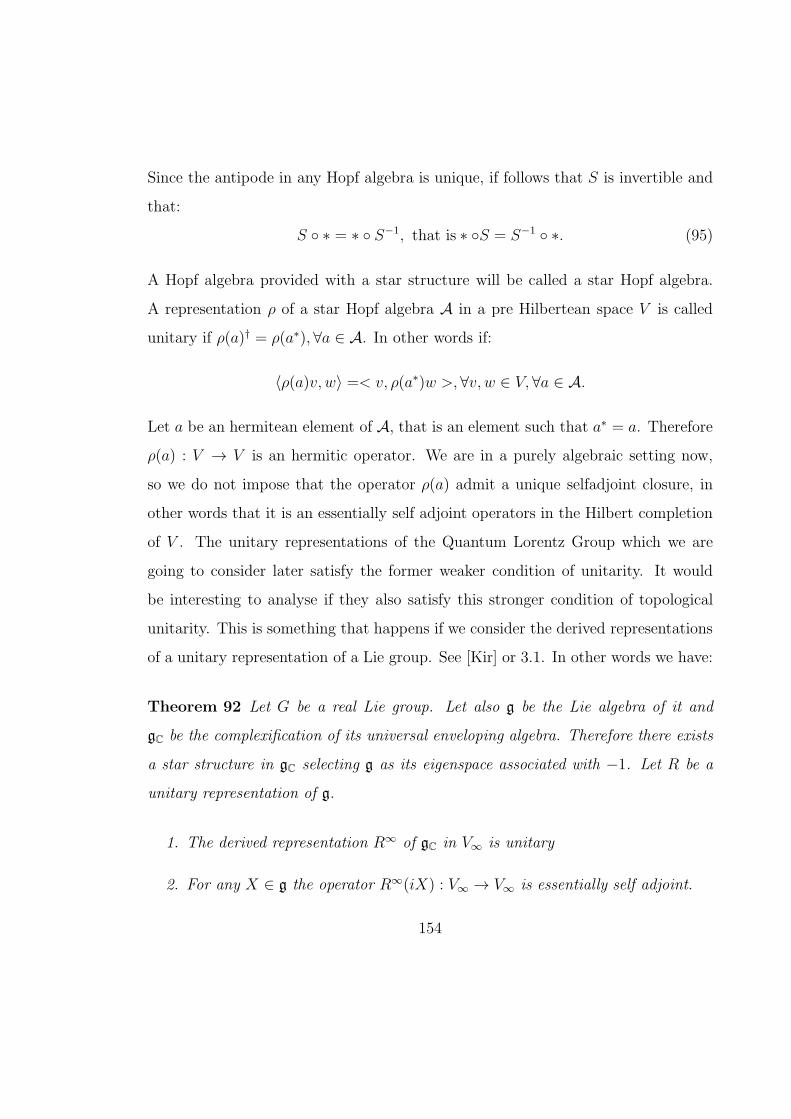
Since the antipode in any Hopf algebra is unique, if follows that S is invertible and
that:
S ∗ = ∗ S−1, that is ∗ S = S−1 ∗. (95)
A Hopf algebra provided with a star structure will be called a star Hopf algebra.
A representation ρ of a star Hopf algebra A in a pre Hilbertean space V is called
unitary if ρ(a)† = ρ(a∗), ∀a ∈ A. In other words if:
〈ρ(a)v, w〉 =< v, ρ(a∗)w >, ∀v, w ∈ V, ∀a ∈ A.
Let a be an hermitean element of A, that is an element such that a∗ = a. Therefore
ρ(a) : V → V is an hermitic operator. We are in a purely algebraic setting now,
so we do not impose that the operator ρ(a) admit a unique selfadjoint closure, in
other words that it is an essentially self adjoint operators in the Hilbert completion
of V . The unitary representations of the Quantum Lorentz Group which we are
going to consider later satisfy the former weaker condition of unitarity. It would
be interesting to analyse if they also satisfy this stronger condition of topological
unitarity. This is something that happens if we consider the derived representations
of a unitary representation of a Lie group. See [Kir] or 3.1. In other words we have:
Theorem 92 Let G be a real Lie group. Let also g be the Lie algebra of it and
gC be the complexification of its universal enveloping algebra. Therefore there exists
a star structure in gC selecting g as its eigenspace associated with −1. Let R be a
unitary representation of g.
1. The derived representation R∞ of gC in V∞ is unitary
2. For any X ∈ g the operator R∞(iX) : V∞ → V∞ is essentially self adjoint.
154

Part 1 of this theorem justifies looking at unitary representations of the quantum
Lorentz group as being quantised counterparts of unitary representations of the
Lorentz Group. In the quantised version of the thery it is also natural to consider
the following compactibility restriction:
Definition 93 Let A be a star Hopf algebra with an R-matrix R ∈ A⊗A. We say
that R is compactible10 with the star structure if R∗⊗∗ = R−1.
One reason to consider this compatibility relation is:
Proposition 94 Let ρ be a unitary representation of A in the pre hilbertean space
V . If R is compactible with ∗ then the braiding operators:
BV,V : v ⊗ w ∈ V ⊗ V 7→ R21(w ⊗ v) ∈ V ⊗ V
are unitary, in other words:
〈BV,V (v ⊗ w), BV,W (v′ ⊗ w′)〉 = 〈v ⊗ w, v′ ⊗ w′〉 .
Therefore they uniquely extend to a topologically unitary map V ⊗ V → V ⊗ V where
V ⊗ V is the Hilbert completion of V ⊗ V .
7.1.2 The algebra Uq(su(2)) and Clebsch-Gordan Coefficients
Let q ∈ (0, 1). The reason why we make this restriction concernes the fact that the
star structure whihch we are going to consider in Uq(su(2)) only makes sense if q is
real and not 0, 1,−1, so we are merely taking a connected component of this set,
10Majid call these quasitriangular structures anti-real as oposed to real ones for which R∗,∗ =
R21. For example if q is real, the usual R-matrix of Uq(su(2)) is real. See [M] and bellow
155

probably an artificial restriction. Consider the Hopf algebra Uq(su(2)) as defined
for example in [BR2]. It is the unital star Hopf algebra defined by the generators
J+, J−, qJz and q−Jz with relations:
q±Jzq∓Jz = 1, qJzJ±q−Jz = q±1J±, [J+, J−] =
q2Jz − q−2Jz
q − q−1, (96)
∆(q±Jz) = q±Jz ⊗ q±Jz , ∆(J±) = q−Jz ⊗ J± + J± ⊗ qJz , (97)
S(q±Jz) = q∓Jz , S(qJ±) = −q±1J∓, (98)
ε(q±Jz) = 1, ε(J±) = 0, (99)
(q±Jz)∗ = q±Jz , J∗± = q∓1J∓. (100)
Notice it is a slightly unstandard definition, but this will not affect our discussion.
This algebra is denoted by Uq(su(2) in [KS]. It is a semisimple algebra, that is any
finite dimensional representation of it can be expressed uniquely as a direct sum
of irreducibles. The irreducible finite dimensional representations of Uq(su(2)) are
classified by a w ∈ 1,−1, i,−i and an α ∈ 12N0. We denote these irreducible
representations by ραw. The representations ρ
αof spin α ∈ 1
2N0 are, by definition, the
ones for which w = 1. They are the natural quantisation of the representations of
su(2) of spin α. The representation space for the representation ραw is V
α
w, a complex
vector space with dimension 2α+1. There exists a basis vα−α, ..., vαa of Vα
w on which
the expression of the representations ραw is:
q±Jzvαiα = wq±iαv
αiα (101)
J+vαiα = wq−
12
√
[α + iα + 1][α− iα]vαiα+1 (102)
J−vαiα = wq+
12
√
[α− iα + 1][α+ iα]vαiα−1 (103)
156

Where the quantum integers [n]q = [n] are defined as [n] = q−n−qnq−1−q . Notice that
the four unique irreducible representations of dimension 2α + 1 of Uq(su(2)) are
distinguished by the spectrum of qJz . This fact will be useful later on.
Let Vα
= Vα
w be the representation space of the representation of spin α. The rep-
resentations ραare unitary under an inner product in V
α
such that vα−α, ..., vαa is an
orthonormal basis. We need to assume q ∈ (0, 1) for this to hold, and actually for
the star structure in Uq(su(2)) to be well defined in the first place. The quantum
dimension of the representation ραis dα = [2α+1]q. The representation of spin zero
is the representation on C such that aλ = ε(a)λ, a ∈ Uq(su(2))λ ∈ C.
Similarly to the classical case, the representations Vα
are closed under taking tensor
products and direct sums in the sense:
Vα
⊗ Vβ ∼=
α+β⊕
γ=|α−β|Vγ
. (104)
There exist thus intertwiners Ψα,βγ : V
α
⊗ Vβ
→ Vγ
and Φγα,β : Vγ
→ Vα
⊗ Vβ
called the
Clebsch-Gordan maps. They are defined apart from phases, but after making some
natural choices there is a well determined one. All this is described in [BR2] and
[KS]. We define the Clebsch-Gordan coefficients as:
Ψα,βγ (v
αiα ⊗ v
βiβ) =
∑
iγ
iγ
γ
α β
iα iβ
vγiγ , (105)
and
Φγα,β(vγiγ ) =
∑
ia,ib
iα iβ
α β
γ
iγ
vαiα ⊗ v
βiβ . (106)
Under the phases chosen in [BR2] they are always real. Let Y (α, β, γ) = 1 if Vα
is
in the decomposition of Vβ
⊗ Vγ
as a direct sums of irreducibles, and zero otherwise.
157
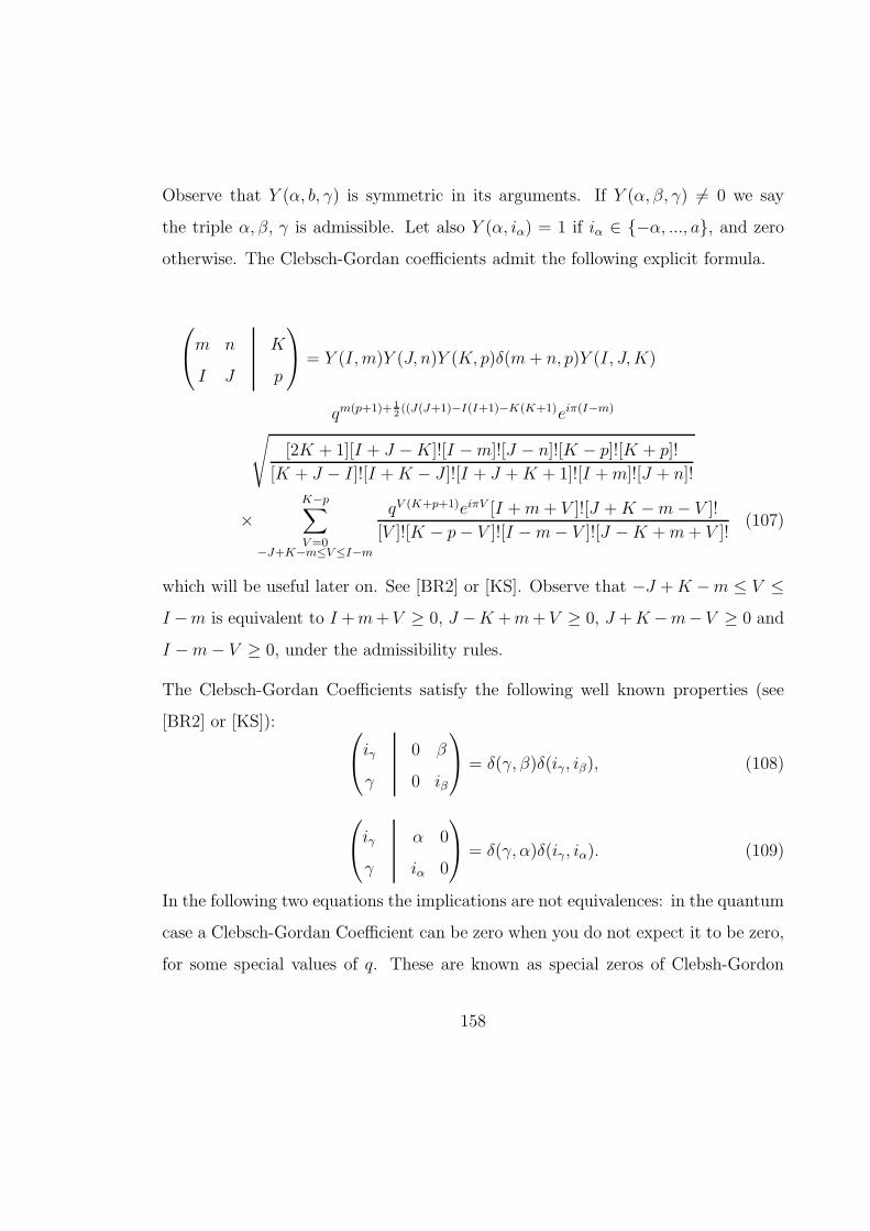
Observe that Y (α, b, γ) is symmetric in its arguments. If Y (α, β, γ) 6= 0 we say
the triple α, β, γ is admissible. Let also Y (α, iα) = 1 if iα ∈ −α, ..., a, and zero
otherwise. The Clebsch-Gordan coefficients admit the following explicit formula.
m n
I J
K
p
= Y (I,m)Y (J, n)Y (K, p)δ(m+ n, p)Y (I, J,K)
qm(p+1)+ 12((J(J+1)−I(I+1)−K(K+1)eiπ(I−m)
√
[2K + 1][I + J −K]![I −m]![J − n]![K − p]![K + p]!
[K + J − I]![I +K − J ]![I + J +K + 1]![I +m]![J + n]!
×K−p∑
V=0−J+K−m≤V≤I−m
qV (K+p+1)eiπV [I +m+ V ]![J +K −m− V ]!
[V ]![K − p− V ]![I −m− V ]![J −K +m+ V ]!(107)
which will be useful later on. See [BR2] or [KS]. Observe that −J +K −m ≤ V ≤I −m is equivalent to I +m+ V ≥ 0, J −K +m+ V ≥ 0, J +K −m− V ≥ 0 and
I −m− V ≥ 0, under the admissibility rules.
The Clebsch-Gordan Coefficients satisfy the following well known properties (see
[BR2] or [KS]):
iγ
γ
0 β
0 iβ
= δ(γ, β)δ(iγ, iβ), (108)
iγ
γ
α 0
iα 0
= δ(γ, α)δ(iγ, iα). (109)
In the following two equations the implications are not equivalences: in the quantum
case a Clebsch-Gordan Coefficient can be zero when you do not expect it to be zero,
for some special values of q. These are known as special zeros of Clebsh-Gordon
158
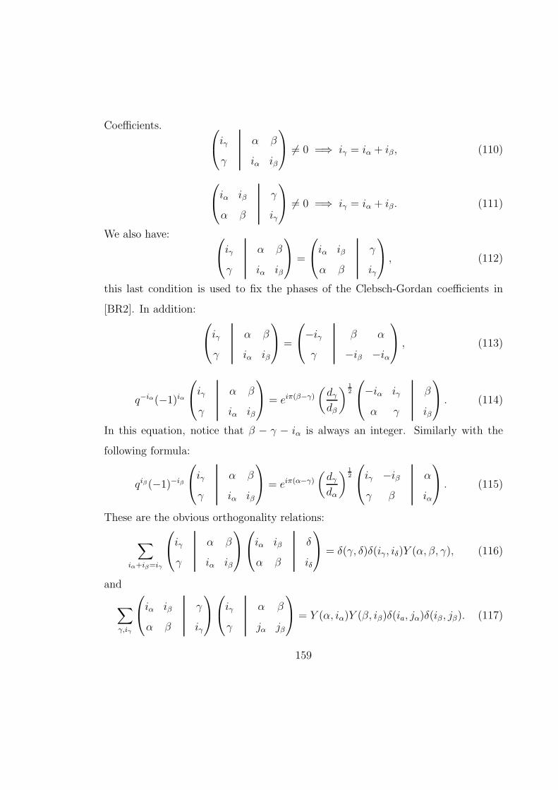
Coefficients.
iγ
γ
α β
iα iβ
6= 0 =⇒ iγ = iα + iβ, (110)
iα iβ
α β
γ
iγ
6= 0 =⇒ iγ = iα + iβ. (111)
We also have:
iγ
γ
α β
iα iβ
=
iα iβ
α β
γ
iγ
, (112)
this last condition is used to fix the phases of the Clebsch-Gordan coefficients in
[BR2]. In addition:
iγ
γ
α β
iα iβ
=
−iγγ
β α
−iβ −iα
, (113)
q−iα(−1)iα
iγ
γ
α β
iα iβ
= eiπ(β−γ)(
dγdβ
)12
−iα iγ
α γ
β
iβ
. (114)
In this equation, notice that β − γ − iα is always an integer. Similarly with the
following formula:
qiβ(−1)−iβ
iγ
γ
α β
iα iβ
= eiπ(α−γ)(
dγdα
)12
iγ −iβγ β
α
iα
. (115)
These are the obvious orthogonality relations:
∑
iα+iβ=iγ
iγ
γ
α β
iα iβ
iα iβ
α β
δ
iδ
= δ(γ, δ)δ(iγ, iδ)Y (α, β, γ), (116)
and
∑
γ,iγ
iα iβ
α β
γ
iγ
iγ
γ
α β
jα jβ
= Y (α, iα)Y (β, iβ)δ(ia, jα)δ(iβ , jβ). (117)
159

Observe that since the Clebsch-Gordan coefficients are real, (116) together with
(112) ensure that their norm is smaller than 1. In some particular cases, the expres-
sion for Clebsch-Gordan coefficients simplifies dramatically. For example:
0
0
A B
m −m
=eiπ(B−m)
√dB
δ(A,B)qm. (118)
7.1.3 6j-symbols and their symmetries
Again we follow the conventions of [BR2]. All the material here can be easily found
in the literature, so we stick to the minimum essential. See [KS] for proofs. Consider
the space of Uq(su(2)) intertwiners Vα
⊗ Vβ
→ Vγ
⊗ Vβ
its has two basis, namely
φεγ,δψα,βε , Y (α, β, ε), Y (γ, δ, ε) = 1
,
and(
idV
γ ⊗ ψωβδ
)(
φαγω ⊗ idV
β
)
, Y (α, γ, ω), Y (ω, β, δ) = 1
.
The 6j-symbols are defined as
∑
ε
γ ω
β ε
α
δ
φεγ,δψα,βε =
(
idV
γ ⊗ ψω bδ
)(
φαγω ⊗ idV
β
)
, (119)
with the convention
γ ω
β ε
α
δ
= 0 if Y (ε, γ, β) = 0 or Y (ε, α, b) = 0.
Therefore
A B
D E
C
F
= Y (A,B,C)Y (C,D,E)Y (A,E, F )Y (D,B, F )
A B
D E
C
F
.
(120)
160
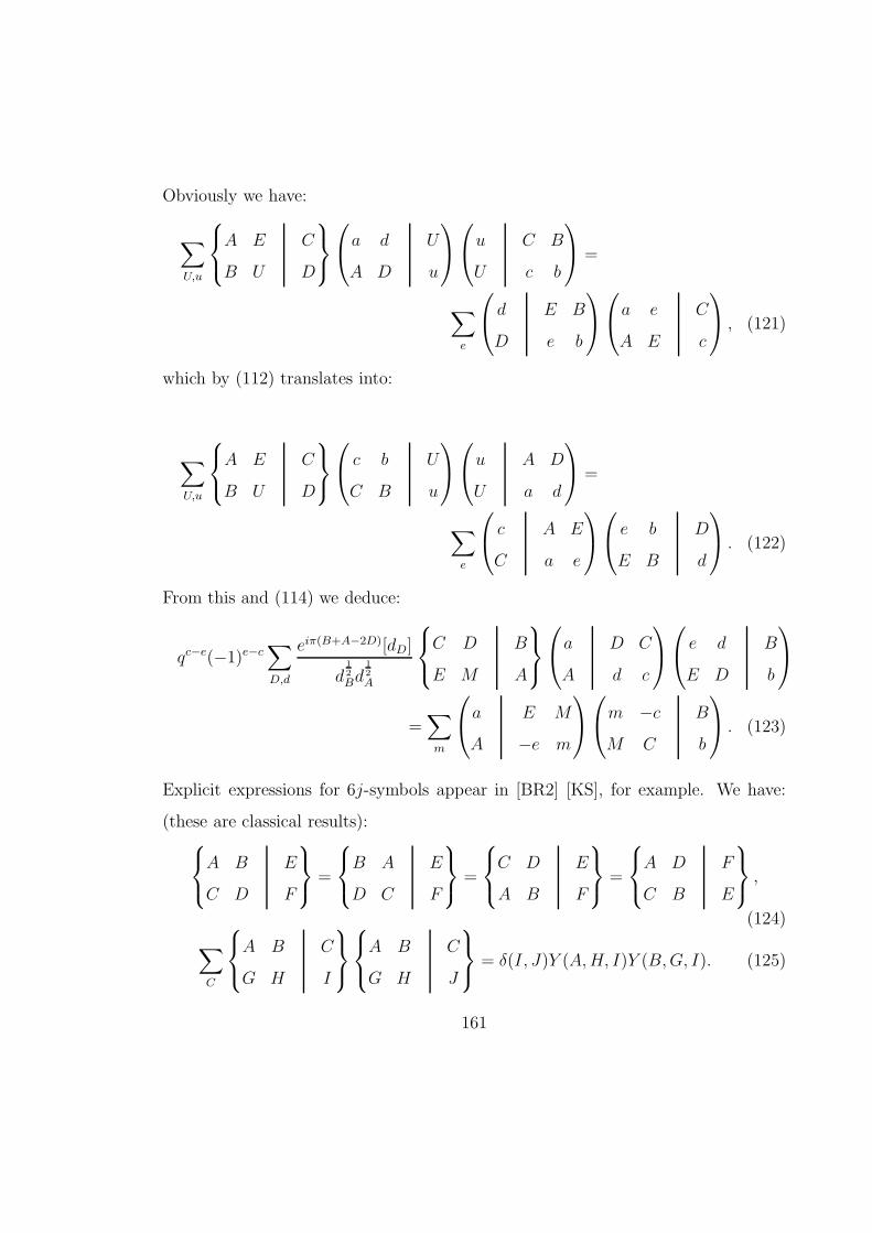
Obviously we have:
∑
U,u
A E
B U
C
D
a d
A D
U
u
u
U
C B
c b
=
∑
e
d
D
E B
e b
a e
A E
C
c
, (121)
which by (112) translates into:
∑
U,u
A E
B U
C
D
c b
C B
U
u
u
U
A D
a d
=
∑
e
c
C
A E
a e
e b
E B
D
d
. (122)
From this and (114) we deduce:
qc−e(−1)e−c∑
D,d
eiπ(B+A−2D)[dD]
d12Bd
12A
C D
E M
B
A
a
A
D C
d c
e d
E D
B
b
=∑
m
a
A
E M
−e m
m −cM C
B
b
. (123)
Explicit expressions for 6j-symbols appear in [BR2] [KS], for example. We have:
(these are classical results):
A B
C D
E
F
=
B A
D C
E
F
=
C D
A B
E
F
=
A D
C B
F
E
,
(124)
∑
C
A B
G H
C
I
A B
G H
C
J
= δ(I, J)Y (A,H, I)Y (B,G, I). (125)
161
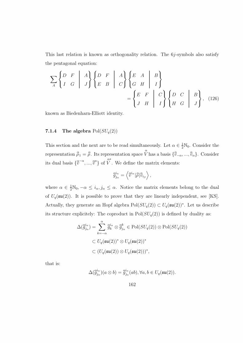
This last relation is known as orthogonality relation. The 6j-symbols also satisfy
the pentagonal equation:
∑
A
D F
I G
A
J
D F
E B
A
C
E A
G H
B
I
=
E F
J H
C
I
D C
H G
B
J
, (126)
known as Biedenharn-Elliott identity.
7.1.4 The algebra Pol(SUq(2))
This section and the next are to be read simultaneously. Let α ∈ 12N0. Consider the
representation ρα1 = ρ
α. Its representation space V
α
has a basis vα−α, ..., vαα. Considerits dual basis vα−α, ..., vαa of V
α∗. We define the matrix elements:
gαiαjα =
⟨
vαiα|ρα|vαiβ
⟩
,
where α ∈ 12N0,−α ≤ iα, jα ≤ α. Notice the matrix elements belong to the dual
of Uq(su(2)). It is possible to prove that they are linearly independent, see [KS].
Actually, they generate an Hopf algebra Pol(SUq(2)) ⊂ Uq(su(2))∗. Let us describe
its structure explicitely: The coproduct in Pol(SUq(2)) is defined by duality as:
∆(gαiαjα) =
α∑
k=−αgαiαk ⊗ g
αkjα ∈ Pol(SUq(2))⊗ Pol(SUq(2))
⊂ Uq(su(2))∗ ⊗ Uq(su(2))
∗
⊂ (Uq(su(2))⊗ Uq(su(2)))∗,
that is:
∆(gαiαjα)(a⊗ b) = g
αiαjα(ab), ∀a, b ∈ Uq(su(2)).
162

The product in Pol(SUq(2)) is the convolution product in Uq(su(2))∗, in other words:
gαiαjαgβiβ
jβ=∑
γ,iγ ,jγ
iα iβ
α β
γ
iγ
jγ
γ
α β
jα jβ
gγiγjγ . (127)
This means:
(
gαiαjαgβiβ
jβ
)
(a) =(
gαiαjα ⊗ g
βiβ
jβ
)
(∆(a)) =⟨
vαiα ⊗ v
βiβ |(ρα⊗ ρβ)(a)|vαjα ⊗ v
βjβ
⟩
, ∀a ∈ Uq(su(2)).
The identity for the product is g00
0. Notice g00
0(a) = ε(a), ∀a ∈ Uq(su(2)), by definition
of the representation of spin 0 Also ε(
gαiαjα
)
= gαiαjα(1) = δ(iα, jα).
The antipode is defined as S(gαiαjα)(a) = g
αiαjα(S(a)), ∀a ∈ Uq(su(2)). It is not imme-
diate that S(gαiαjα) ∈ Pol(SUq(2)). Let us explain why it is so: Let α ∈ 1
2N0, and
consider the representation ραin V
α
. Its conjugate representation (ρα) is the represen-
tation in the conjugate vector space Vα
given by ρα(a) = ρ
α(S−1(a∗)), ∀a ∈ Uq(su(2)).
The conjugate vector space Vα
admits the basis vα−α, ..., vαα. An easy calculation
shows that ραis equivalent to ρ
αand that an intertwiner is: v
αiα 7→ q−iα(−1)α−iαv
α−iα.
See [BR2]. We thus have:
⟨
vαiα |ρα(S(a))|vαjα
⟩
=⟨
vαjα|ρα(S(a)∗)|vαiα
⟩
, since ραis unitary
(128)
=⟨
vαjα|ρα(S−1(a∗))|vαiα
⟩
, from equation (95)
(129)
=⟨
vαjα|ρα(a)|vαiα
⟩
, by definition
(130)
=⟨
vα−jα|ρα(a)|vα−iα
⟩
qiα−jα(−1)−iα+jα. (131)
In particular
S(gαiαjα) = qiα−jα(−1)−iα+jαg
α−jα−iα ∈ Pol(SUq(2)), (132)
163

if α ∈ 12N0 and iα, jα ∈ −α, ..., α. Observe that S is indeed an antipode for
Pol(SUq(2)), since for any a ∈ Uq(su(2)) we have:
∑
(gαiα
jα)
S(gαiαjα
′)gαiαjα
′′(a) =
∑
(a)
(
S(gαiαjα
′)gαiαjα
′′)(a′ ⊗ a′′)
= gαiαjα(∑
(a)
S(a′)a′′)
= ε(a)gαiαjα(1)
= g00
0(a)ε(gαiαjα),
where if A is a Hopf algebra we denote ∆(a) =∑
(a) a′ ⊗ a′′. In particular, given
that the matrix elements gαiαjα ∈ Uq(su(2))
∗ are linearly independent we have:
∑
k
S(gαiαk )g
αkjα = δ(iα, jα)g
00
0,
which implies the following identity satisfied by Clebsch-Gordan coefficients:
∑
r,s,k
−k k
α α
γ
r
s
γ
α α
−iα jα
qiα−k(−1)−iα+k = δ(γ, 0)δ(iα, jα). (133)
It is possible to give a direct proof of it using the properties of the Clebsch-Gordan
coeefficients given before, namely (116) and (118).
The algebra Pol(SUq(2)) also has a star structure given by f ∗(a) = f(S−1(a∗). Thus
gαiαjα
∗= S(g
αjαiα ) = qjα−iα(−1)iα−jαg
α−iα−jα, (134)
this follows from (128) and following calculations.
Usually the algebra Pol(SUq(2)) is denoted by SUq(2), and can be described in
terms of the generators a, b, c, d and relations as for example in [K], [KS] and also
164
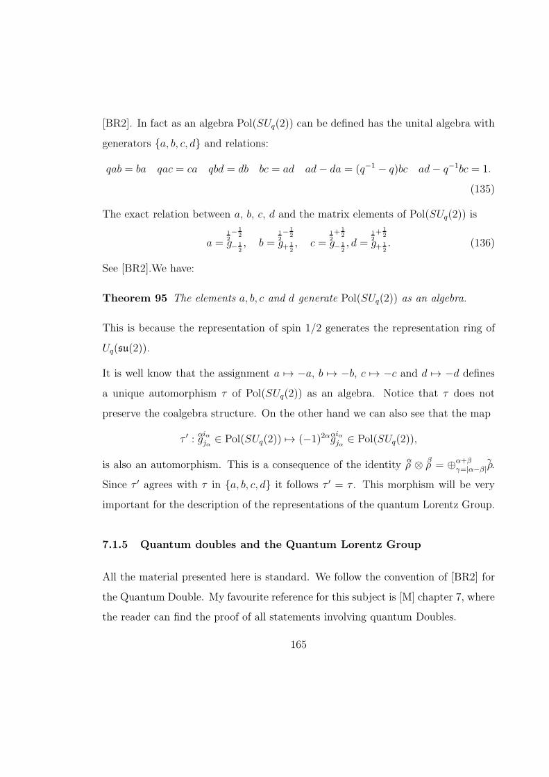
[BR2]. In fact as an algebra Pol(SUq(2)) can be defined has the unital algebra with
generators a, b, c, d and relations:
qab = ba qac = ca qbd = db bc = ad ad− da = (q−1 − q)bc ad− q−1bc = 1.
(135)
The exact relation between a, b, c, d and the matrix elements of Pol(SUq(2)) is
a = g12− 1
2
− 12, b = g
12− 1
2
+ 12, c = g
12+ 1
2
− 12, d = g
12+ 1
2
+ 12. (136)
See [BR2].We have:
Theorem 95 The elements a, b, c and d generate Pol(SUq(2)) as an algebra.
This is because the representation of spin 1/2 generates the representation ring of
Uq(su(2)).
It is well know that the assignment a 7→ −a, b 7→ −b, c 7→ −c and d 7→ −d defines
a unique automorphism τ of Pol(SUq(2)) as an algebra. Notice that τ does not
preserve the coalgebra structure. On the other hand we can also see that the map
τ ′ : gαiαjα ∈ Pol(SUq(2)) 7→ (−1)2αg
αiαjα ∈ Pol(SUq(2)),
is also an automorphism. This is a consequence of the identity ρα ⊗ ρ
β= ⊕α+β
γ=|α−β|ργ.
Since τ ′ agrees with τ in a, b, c, d it follows τ ′ = τ . This morphism will be very
important for the description of the representations of the quantum Lorentz Group.
7.1.5 Quantum doubles and the Quantum Lorentz Group
All the material presented here is standard. We follow the convention of [BR2] for
the Quantum Double. My favourite reference for this subject is [M] chapter 7, where
the reader can find the proof of all statements involving quantum Doubles.
165

Let A = (A, m, 1,∆, ε) be a finite dimensional Hopf algebra. Recall the dual vector
space A can also be given a Hopf algebra structure, where all structure maps in A∗
are defined through dualising the ones of A. For example ∆ : A∗ → A∗ ⊗ A∗ is
defined as the composition
A∗ m∗
−→ (A⊗A)∗∼=−→ A∗ ⊗A∗,
where m∗ is the transpose of the multiplicatio m : A⊗A → A. Whereas (fg)(a) =
(f⊗g)∆(a), where f, g ∈ A∗ and a ∈ A. This product in A∗ is called the convolution
product. It makes sense even in A is infinite dimensional. However the isomorphism
(A ⊗A)∗ ∼= A∗ ⊗ A∗ breaks in the infinite dimensional case, so it is not true that
A∗ has a structure of Hopf algebra, for we cannot define a coproduct. However,
sometimes the problem can be fixed by restricting to a subalgebra of A∗. This wasdone in the previous section defining the algebra Pol(SUq(2)) contained in the dual
of Uq(su(2)).
If A is an Hopf algebra let Acop be the Hopf algebra with the same multiplication,
unit and counit but comultiplication ∆cop(a) =∑
(a) a′′ ⊗ a′, thus the antipode of
Acop is S−1. If A as a star structure then both A∗ and A∗cop have star structures
given by f ∗(a) = f(S−1(a∗)) Let A be a finite dimensional Hopf algebra. The
quantum double of A is denoted by D(A,A∗cop). It is A⊗A∗cop as a vector space
and coalgebra. However the product in D(A,A∗cop) is given by
(x⊗ f)(y ⊗ g)∑
(y),(f)
< f ′′′, S−1(y′) >< f ′, y′′′ > xy′′ ⊗ f ′′g. (137)
The antipode of the quantum double is given by S(a⊗ f) = (1⊗S−1(f))(S(a)⊗ 1).
Here ∆(f) =∑
(f) f′⊗f ′′ and S(f) denote the comultiplication and antipode of A∗.
Let ai be a basis of A and ai the dual basis of A∗. Recall the quantum double
166
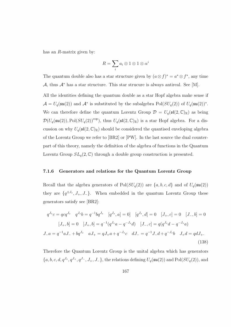
has an R-matrix given by:
R =∑
i
ai ⊗ 1⊗ 1⊗ αi
The quantum double also has a star structure given by (a⊗ f)∗ = a∗⊗ f ∗, any time
A, thus A∗ has a star structure. This star strucure is always antireal. See [M].
All the identities defining the quantum double as a star Hopf algebra make sense if
A = Uq(su(2)) and A∗ is substituted by the subalgebra Pol(SUq(2)) of Uq(su(2))∗.
We can therefore define the quantum Lorentz Group D = Uq(sl(2,C)R) as being
D(Uq(su(2)),Pol(SUq(2))cop), thus Uq(sl(2,C)R) is a star Hopf algebra. For a dis-
cussion on why Uq(sl(2,C)R) should be considered the quantised enveloping algebra
of the Lorentz Group we refer to [BR2] or [PW]. In the last source the dual counter-
part of this theory, namely the definition of the algebra of functions in the Quantum
Lorentz Group SLq(2,C) through a double group construction is presented.
7.1.6 Generators and relations for the Quantum Lorentz Group
Recall that the algebra generators of Pol(SUq(2)) are a, b, c, d and of Uq(su(2))
they are q±Jz , J+, J−. When embedded in the quantum Lorentz Group these
generators satisfy see [BR2]:
qJzc = qcqJz qJzb = q−1bqJz [qJz , a] = 0] [qJz , d] = 0 [J+, c] = 0 [J−, b] = 0
[J+, b] = 0 [J+, b] = q−1(qJza− q−Jzd) [J−, c] = q(qJzd− q−Jza)
J−a = q−1aJ−+ bqJz aJ+ = qJ+a+ q
−Jzc dJ− = q−1J−d+ q−Jzb J+d = qdJ+.
(138)
Therefore the Quantum Lorentz Group is the unital algebra which has generators
a, b, c, d, qJz , qJ+, qJ−, J+, J−, the relations defining Uq(su(2)) and Pol(SUq(2)), and
167
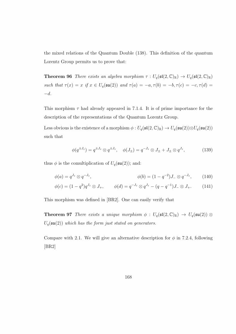
the mixed relations of the Quantum Double (138). This definition of the quantum
Lorentz Group permits us to prove that:
Theorem 96 There exists an algebra morphism τ : Uq(sl(2,C)R) → Uq(sl(2,C)R)
such that τ(x) = x if x ∈ Uq(su(2)) and τ(a) = −a, τ(b) = −b, τ(c) = −c, τ(d) =−d.
This morphism τ had already appeared in 7.1.4. It is of prime importance for the
description of the representations of the Quantum Lorentz Group.
Less obvious is the existence of a morphism φ : Uq(sl(2,C)R) → Uq(su(2))⊗Uq(su(2))such that
φ(q±Jz) = q±Jz ⊗ q±Jz , φ(J±) = q−Jz ⊗ J± + J± ⊗ qJz , (139)
thus φ is the comultiplication of Uq(su(2)); and:
φ(a) = qJz ⊗ q−Jz , φ(b) = (1− q−2)J− ⊗ q−Jz , (140)
φ(c) = (1− q2)qJz ⊗ J+, φ(d) = q−Jz ⊗ qJz − (q − q−1)J− ⊗ J+. (141)
This morphism was defined in [BR2]. One can easily verify that
Theorem 97 There exists a unique morphism φ : Uq(sl(2,C)R) → Uq(su(2)) ⊗Uq(su(2)) which has the form just stated on generators.
Compare with 2.1. We will give an alternative description for φ in 7.2.4, following
[BR2]
168

7.2 An aside on pseudo quasi triangular structures in the
algebra Uq(su(2))
7.2.1 Quasi triangular structure in Uq(su(2)) and associated knot Invari-
ants
Let q ∈ (0, 1). Recall that Uq(su(2)) has an R-matrix given by:
R = q2Jz⊗Jz∞∑
n=0
qn(n+1)
2
[n]!(q − q−1)n(qJzJ+)
n ⊗ (J−q−Jz)n, (142)
with inverse:
R−1 = q−2Jz⊗Jz∞∑
n=0
q−nq
n(n+1)2
[n]!(q − q−1)n(q2JzJ+)
n ⊗ (qJzJ−q−Jz)n. (143)
These infinite sums make sense when applied to the tensor product of two finite
dimensional representations of Uq(su(2)), if they are direct sums of representations
ραw where w = 1. This is because, when considering the action in pair ρ
α⊗ρβof finite
dimensional representations, the infinite sum
∞∑
n=0
qn(n+1)
2
[n]!(q − q−1)n(qJzJ+)
n ⊗ (J−q−Jz)n
truncates to a finite sum. Also, by definition q2Jz⊗Jz(vαiα ⊗ v
βiβ) = q2iαiβv
αiα ⊗ v
βiβ if
vαiα ∈ V
α
1 = Vα
and vβiβ ∈ V
β
. The action of the R-matrix in the other irreducible
representations is ambiguous. We say R is an R-matrix of Uq(su(2)) in the sense
that for any pair of representations ραand ρ
βof Uq(su(2)) the map v
αiα⊗v
βiβ ∈ V
α
⊗Vα
7→R21v
βiβ ⊗ v
αiαVβ
⊗ Vα
is an intertwiner; and that these maps also define a braid group
representation. These issues are better described dually, in other words considering
the action of the r-form of Pol(SUq(2)) in the finite dimensional corepresentations
of it, as we will see in the next section.
169

The Hopf algebra Uq(su(2)) also has a group like element given by G = q2Jz . With
this formal R-matrix and group like element, the Hopf algebra Uq(su(2)) is a ribbon
Hopf algebra. This means that its category of finite dimensional representations
which are direct sums of representations ρα1 = ρ
αis a ribbon category. We thus have
a knot invariant I(ρα)(q) for any α ∈ 1
2N0 and any q ∈ (0, 1). If K is a framed knot,
the assignment q ∈ (0, 1) 7→ I(ρα)(q)(K) expresses as a finite sum of square roots
of rational functions of q, which are well defined close to 1. Thus they define an
analytic function of q in a neighborhood of 1, and in particular a power series in h
through the substitution q = exp(h). Therefore we can interpret these invariants
as taking values in C[[h]]. They relate to the coloured Jones Polynomial. In fact, a
glance at 1.4.1 tells us immediately that:
Lemma 98 For any α ∈ 12N0 and q ∈ (0, 1) we have I(ρ
α)(q1/2)(K) = Jα(K)(h),
for any framed knot K. Here q = exp(h) and h < 0
In other words, the summation of Jα(K)(h) needs to agree with I(ρα)(q1/2)(K) for
q ∈ (0, 1) and close enough to 1. Recall Jα(K)(h) is a power series with an infinite
radius of convergence.
7.2.2 Corepresentations of Pol(SUq(2)) and r-form
A good reference now is [M]. As we have mentioned in the previous section, the
problem arising from the fact the R-matrix of Uq(su(2)) not precisely an R-matrix
can be eliminated by considering the dual picture. Let A be a Hopf algebra. In
particular we can consider the convolution product in A∗ such that (fg)(a) = (f ⊗g)∆(a). Its identity is ε : A → C. An element r ∈ (A⊗ A)∗ is an r-form if it has a
convolution inverse r and:
170

1.∑
(a)(b)
r(a′ ⊗ b′)a′′b′′ =∑
(a)(b)
r(a′′ ⊗ b′′)b′a′, ∀a, b ∈ A,
2.
r(ab, c) =∑
(c)
r(a, c′)r(b, c′′), ∀a, b, c ∈ A,
3.
r(a, bc) =∑
(a)
r(a′, c)r(a′′, b), ∀a, b, c ∈ A.
Consider the bilinear form r in Pol(SUq(2)) given by
r(gαiαjα, g
βiβ
jβ) =
⟨
vαiα ⊗ v
βiβ∣
∣
∣(ρα⊗ ρ
β)(R)
∣
∣
∣vαiα ⊗ v
βiβ
⟩
, (144)
then r is an r-form of Pol(SUq(2)). See [KS], 8.3.3 and 10.1. Its convolution inverse
is:
r−1(gαiαjα, g
βiβ
jβ) =
⟨
vαiα ⊗ v
βiβ∣
∣
∣(ρα⊗ ρ
β)(R−1)
∣
∣
∣vαiα ⊗ v
βiβ
⟩
. (145)
In particular given two corepresentations φ and ψ of Pol(SUq(2)) in V and W there
exists an intertwiner V ⊗W →W ⊗ V . It has the form
V ⊗W x⊗y 7→y⊗x−−−−−−→W⊗V ψ⊗φ−−→W⊗Pol(SUq(2))⊗V ⊗Pol(SUq(2))r24−→W⊗V. (146)
Consider the corepresentations ψa, α ∈ 12N0 of Pol(SUq(2)) in V
α
given by:
vαiα 7→ v
αjα ⊗ g
αjαiα ,
then obviously the intertwiner in (146) is exactly v ⊗ w 7→ R21w ⊗ v. This is prob-
ably the clearest way to understand the R-matrix in Uq(su(2)) in a precise level
when considering representations ρα1 (though not the clearest in the intuitive level).
Analogously, the ribbon category structure in the category of representations of
171

Uq(su(2)) which are direct sums of representations ραcan be understood by consid-
ering the coribbon structure in Pol(SUq(2)), dual to the heuristic ribbon structure
of Uq(su(2)) described for example in [BR2].
It is well know that the corepresentations ψα exhaust all the irreducible corepresen-
tation of Pol(SUq(2)) and that any corepresentation of it expresses as a direct sum
of these. Therefore, the representations ραw of Uq(su(2)) with w 6= 1 are not dual
to any correpresentation of Pol(SUq(2)). This is the reason why the triangular and
ribbon structures in the representations ραw with w = 1 do not extend to all finite
dimensional representations of Uq(su(2)).
The algebra Uq(su(2)) is a subalgebra of the dual Pol(SUq(2))∗ of Pol(SUq(2)), the
last given the convolution product. It is not difficult to verify that:
Proposition 99 For any α ∈ 12N0 and any −α ≤ iα, iβ ≤ α the map
f ∈ Pol(SUq(2)) 7→ r(gαiαjα, f) ∈ C
is in Uq(su(2)), considering the embedding Uq(su(2)) → Pol(SUq(2))∗. Therefore it
defines a map Pol(SUq(2)) → Uq(su(2)) which we denote by: g 7→ (g ⊗ id)(R).
We thus have < vβiβ |(gαiαjα ⊗ id)(R)v
βiβ >=< (g
αiαjα ⊗ id)(R), g
βiβ
jβ>= r(g
αiαjα, g
βiβ
jβ), by defi-
nition. Actually, this map is a morphism. This is because for any f ∈ Pol(SUq(2))
we have:
< (gh⊗ id)(R), f > = r(gh, f)
=∑
(f)
r(g, f ′)r(h, f ′′)
=< (g ⊗ id)(R), f ′ >< (h⊗ id)(R), f ′′ >
=< (g ⊗ id)(R)(h⊗ id)(R), f > .
172

We can derive some other identities, which will be useful in 7.3.8. Let f, g, h ∈Pol(SUq(2)). We thus have
∑
(f)
< (f ′ ⊗ id)(R), g >< (f ′′ ⊗ id)(R), h > =∑
(f)
r(f ′, g)r(f ′′, h)
= r(f, hg)
=< (f ⊗ id)(R), hg > .
Let R(−) = R−121 . If f ∈ Pol(SUq(2)), we can define analogously (f ⊗ id)(R(−)) ∈Uq(su(2)). In particular < (f ⊗ id)(R(−), g >= r−121 (f, g) = r(f, g). Let f, g, h ∈Pol(SUq(2)). We have
∑
(f)
< (f ′ ⊗ id)(R), g >< (f ′′ ⊗ id)(R(−)), h > =∑
(f)
r(f ′, g)r(f ′′, h)
= r12r13(f, g, h)
.
The last equality follows by definition of the convolution product in Pol(SUq(2))∗.
7.2.3 Quantum co-double of quasitriangular Hopf algebras and knot in-
variants
The best reference now for general quantum group theory is still [M], chapter 7.
Let A be a Hopf algebra with an R-matrix R. The quantum co-double A⊗A of Ais defined as the Hopf algebra which has A ⊗ A has underlying algebra and with
counit ε⊗ ε. The modified coproduct is:
∆(a⊗ b) = R−123 a′ ⊗ b′ ⊗ a′′ ⊗ b′′R23,
whereas the antipode is defined as:
173
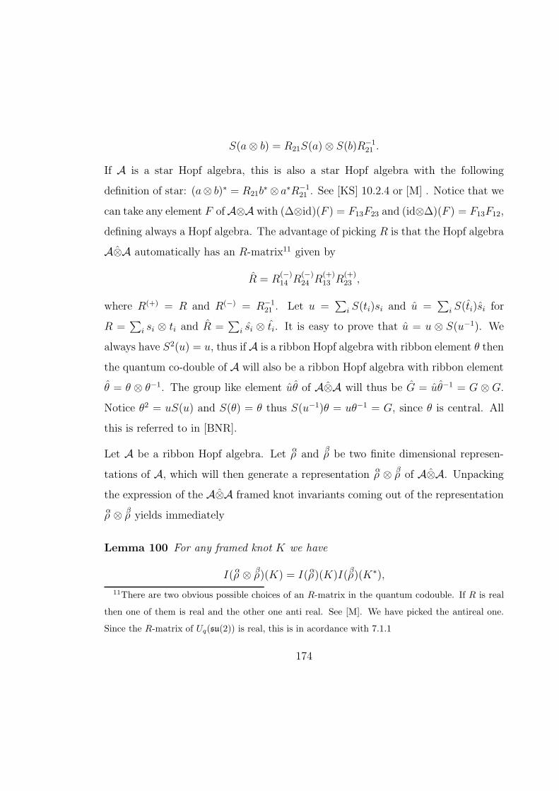
S(a⊗ b) = R21S(a)⊗ S(b)R−121 .
If A is a star Hopf algebra, this is also a star Hopf algebra with the following
definition of star: (a⊗ b)∗ = R21b∗⊗ a∗R−121 . See [KS] 10.2.4 or [M] . Notice that we
can take any element F ofA⊗A with (∆⊗id)(F ) = F13F23 and (id⊗∆)(F ) = F13F12,
defining always a Hopf algebra. The advantage of picking R is that the Hopf algebra
A⊗A automatically has an R-matrix11 given by
R = R(−)14 R
(−)24 R
(+)13 R
(+)23 ,
where R(+) = R and R(−) = R−121 . Let u =∑
i S(ti)si and u =∑
i S(ti)si for
R =∑
i si ⊗ ti and R =∑
i si ⊗ ti. It is easy to prove that u = u ⊗ S(u−1). We
always have S2(u) = u, thus ifA is a ribbon Hopf algebra with ribbon element θ then
the quantum co-double of A will also be a ribbon Hopf algebra with ribbon element
θ = θ ⊗ θ−1. The group like element uθ of A⊗A will thus be G = uθ−1 = G ⊗ G.
Notice θ2 = uS(u) and S(θ) = θ thus S(u−1)θ = uθ−1 = G, since θ is central. All
this is referred to in [BNR].
Let A be a ribbon Hopf algebra. Let ραand ρ
βbe two finite dimensional represen-
tations of A, which will then generate a representation ρα ⊗ ρ
βof A⊗A. Unpacking
the expression of the A⊗A framed knot invariants coming out of the representation
ρα⊗ ρ
βyields immediately
Lemma 100 For any framed knot K we have
I(ρα⊗ ρ
β)(K) = I(ρ
α)(K)I(ρ
β)(K∗),
11There are two obvious possible choices of an R-matrix in the quantum codouble. If R is real
then one of them is real and the other one anti real. See [M]. We have picked the antireal one.
Since the R-matrix of Uq(su(2)) is real, this is in acordance with 7.1.1
174

Figure 30: A knot K and K∗ ∪K
where K∗ is the mirror image of K.
This is because I(ρα)(K)I(ρ
β)(K)) equals theA-knot invariant evaluated inK∪K∗ for
K coloured with ραandK∗ coloured with ρ
β. We suppose thatK∗ is placed away from
K as in figure 30. It is also important to remember that S(a⊗b) = R21S(a)⊗S(b)R−121
in the quantum co-double. This lemma is used implicitly in [BR2] and [BNR] for
several times. For the ones who want more details: A good way to prove this lemma
precisely is to use the fact that if a knot is the closure of a braid b with n strands
and ρ is a representation in V , then I(ρ)(K) = trv ∈ V ⊗n 7→ G⊗nR(b)(v), whereR(b) is the braiding operator V ⊗n → V ⊗n. This expression works for any ribbon
Hopf algebra. Therefore the lemma is obvious from the form of the R-matrix of
A⊗A is R = R(−)14 R
(−)24 R
(+)13 R
(+)23 and the fact G = G⊗G.
In the Uq(su(2)) case things are slightly more complicated. We can define the
175

coevaluation map by considering the action of Uq(su(2)) in its finite dimensional
representations. We can do the same for the antipodal map. The point is that
tensor products and duals of representations of Uq(su(2))⊗Uq(su(2)) are perfectly
well defined. Thus formally Uq(su(2))⊗Uq(su(2)) is still a ribbon Hopf algebra, in
the sense that the representations of it which are direct sums of representations
ρα ⊗ ρ
βis a ribbon category. This follows from the fact Uq(su(2)) with its formal
R-matrix and group like element G is a ribbon category. The group like element
of Uq(su(2))⊗Uq(su(2)) is G ⊗ G, where G = q2Jz is the group like element of
Uq(su(2)). A good way to present this arguments in a cleaner way is again to consider
the dual picture. Namely the dual construction with the r-form of Pol(SUq(2))
yields an Hopf algebra isomorphic with Pol(SUq(2))⊗ Pol(SUq(2)) as a co-algebra,
whereas the product is the generalised quantum double 12 relative to the pairing
r : Pol(SUq(2)) ⊗ Pol(SUq(2)) → C. This Hopf algebra has an r-form given by
r−141 r−124 r13r23. See [KS] 10.2.3 13.
We can calculate knot invariants from Uq(su(2))⊗Uq(su(2)), and any representations
ρα ⊗ ρ
βof it. Denote this invariant by I(ρ
α ⊗ ρβ). By lemmas 98 and 100 it follows
that:
Lemma 101 For any α, β ∈ 12N0 we have:
I(ρα⊗ ρ
β)(q1/2) = Lα,β(K)(−h),
where q = (0, 1) and exp(h) = q for h < 0.
Recall 3.3.3 and that Lα,β(K)(q) is a convergent power series if α, β ∈ 12N0. Notice
12The simpler case considered before was made out of the canonical dual pairing between an
algebra and its dual13Notice similarly that this generalised quantum double has two natural r-forms
176

that in the notation of chapter 2 we have:
Lα,β(K)(h) = X(α− β, α + β + 1)(2α + 1)(2β + 1)
from Theorem 16.
7.2.4 The quantum co-double of Uq(su(2)) and the Quantum Lorentz
Group
Suppose A is a finite dimensional Hopf algebra with an R-matrix R. There exists a
natural vector space map φ : D(A,A∗cop) 7→ A⊗A. It has the form:
φ : (x⊗ f) 7→∑
(x)(f)
x′(f ′′ ⊗ id)(R(+))⊗ x′′(f ′ ⊗ id)(R(−)) = φ(x)φ(y). (147)
The coevaluations are taken in A and A∗ (not in A∗cop). The map φ transforms
the R-matrix of the quantum double in the R-matrix of A⊗A. This is an easy
consequence of the fact (∆ ⊗ id)(R) = R13R23 = (id ⊗∆)(R) = R13R12 for any R-
matrix R, from which follows (∆⊗ id)(R(−)) = R(−)13 R
(−)23 . Indeed let R =
∑
i si ⊗ ti
and R−1 =∑
i si ⊗ ti. The R-matrix of the quantum double is∑
kXk ⊗ 1⊗ 1⊗Xk
where Xk is a basis of A and Xk its dual basis of A∗. We have
(φ⊗ φ)(R) = (φ⊗ φ)(∑
k
Xk ⊗ 1⊗ 1⊗Xk)
=∑
k,(Xk),i,j
∆(Xk)⊗Xk′′(si)ti ⊗Xk′(tj)sj
=∑
i,j,k
∆(Xk)⊗Xk(tjsi)tj ⊗ sj
= (∆⊗ id)(R(−)13 R
(+)12 )
= R(−)14 R
(−)24 R
(+)13 R
(+)23 .
177

=
Figure 31: An equality between two braids
For the third equality, notice that A is isomorphic with A∗∗, the last given the
convolution product. In particular < a⊗ b,∆(f) >=< ab, f >, ∀a, b ∈ A, ∀f ∈ A∗.The map φ is always a morphism of Hopf algebras algebras. This is shown in [M]
(Theorem 7.3.5), for instance. It is not totally trivial. For the comultiplication for
example, the difficult part is to prove that ∆(φ(g)) = (φ⊗ φ)(∆(g)), if g ∈ A∗. LetR =
∑
i si⊗ti andR−1 =∑
i si⊗ti. Notice φ(g) =∑
i,j g(tjsi)ti⊗sj . We have (notice
it is the co-algebra A∗cop which is embedded in D, not A, thus ∆D(g) =∑
(g) g′′⊗g′):
∆(φ(g)) =∑
i,j,k,l,(ti),(sj)
g(tjsi)t′i ⊗ sksj
′sl ⊗ tkt′′i tl ⊗ s′′j ,
whereas
(φ⊗ φ)∆(g) =∑
i,j,k,l
g(tksltj si)ti ⊗ sj ⊗ tl ⊗ sk
The fact the two expressions are equal is a consequence of Mac Lane’s coherence
theorem for braided tensor categories. See figure 31.
The identities (S ⊗ S)(R) = R and (S ⊗ S) ∆ = ∆cop S, and a similar argument
178
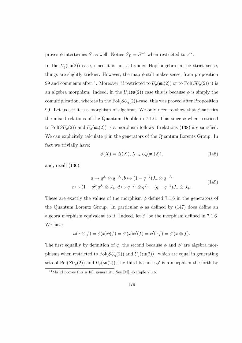
proves φ intertwines S as well. Notice SD = S−1 when restricted to A∗.
In the Uq(su(2)) case, since it is not a braided Hopf algebra in the strict sense,
things are slightly trickier. However, the map φ still makes sense, from proposition
99 and comments after14. Moreover, if restricted to Uq(su(2)) or to Pol(SUq(2)) it is
an algebra morphism. Indeed, in the Uq(su(2)) case this is because φ is simply the
comultiplication, whereas in the Pol(SUq(2))-case, this was proved after Proposition
99. Let us see it is a morphism of algebras. We only need to show that φ satisfies
the mixed relations of the Quantum Double in 7.1.6. This since φ when restriced
to Pol(SUq(2)) and Uq(su(2)) is a morphism follows if relations (138) are satisfied.
We can explicitely calculate φ in the generators of the Quantum Lorentz Group. In
fact we trivially have:
φ(X) = ∆(X), X ∈ Uq(su(2)), (148)
and, recall (136):
a 7→ qJz ⊗ q−Jz , b 7→ (1− q−2)J− ⊗ q−Jz
c 7→ (1− q2)qJz ⊗ J+, d 7→ q−Jz ⊗ qJz − (q − q−1)J− ⊗ J+.(149)
These are exactly the values of the morphism φ defined 7.1.6 in the generators of
the Quantum Lorentz Group. In particular φ as defined by (147) does define an
algebra morphism equivalent to it. Indeed, let φ′ be the morphism defined in 7.1.6.
We have
φ(x⊗ f) = φ(x)φ(f) = φ′(x)φ′(f) = φ′(xf) = φ′(x⊗ f).
The first equalily by definition of φ, the second because φ and φ′ are algebra mor-
phisms when restricted to Pol(SUq(2)) and Uq(su(2)) , which are equal in generating
sets of Pol(SUq(2)) and Uq(su(2)), the third because φ′ is a morphism the forth by
14Majid proves this is full generality. See [M], example 7.3.6.
179

the definition of multiplication in the Quantum Double. Thus it follows φ = φ′ and
since φ′ is a morphism φ is as well.
The existence of this Hopf algebra morphism φ was stated in [BR2], however in the
way it is stated it is not clear that everything works for we only have an heuristic
R-matrix in Uq(su(2)). This construction is one of the major tools for proving the
main theorems of this chapter, the reason why I presented it here with all this detail.
This is also proved in [M], as we have referred to before.
The morphism φ : Uq(sl(2,C)R) → Uq(su(2))⊗Uq(su(2)) gives us a representation of
the Quantum Lorentz Group for any pair of representation of Uq(su(2)). We shall
go back to this in 7.3.1.
7.3 Representations of the Quantum Lorentz Group
We now look at the representation theory of the quantum Lorentz group. We base
our approach on examples, with the final aim of describing the knot theory coming
out of them. The main reference is [BR2].
7.3.1 Crossed Pol(SUq(2))-bimodules and finite dimensional representa-
tions of the Quantum Lorentz Group
A class of finite dimensional representations of the quantum Lorentz Group arises if
we consider Pol(SUq(2))-crossed bimodules. A crossed bimodule is a finite dimen-
sional complex vector space V provided with a left representation of Pol(SUq(2))
and a right corepresentation of Pol(SUq(2)). They need to be compactible in the
180
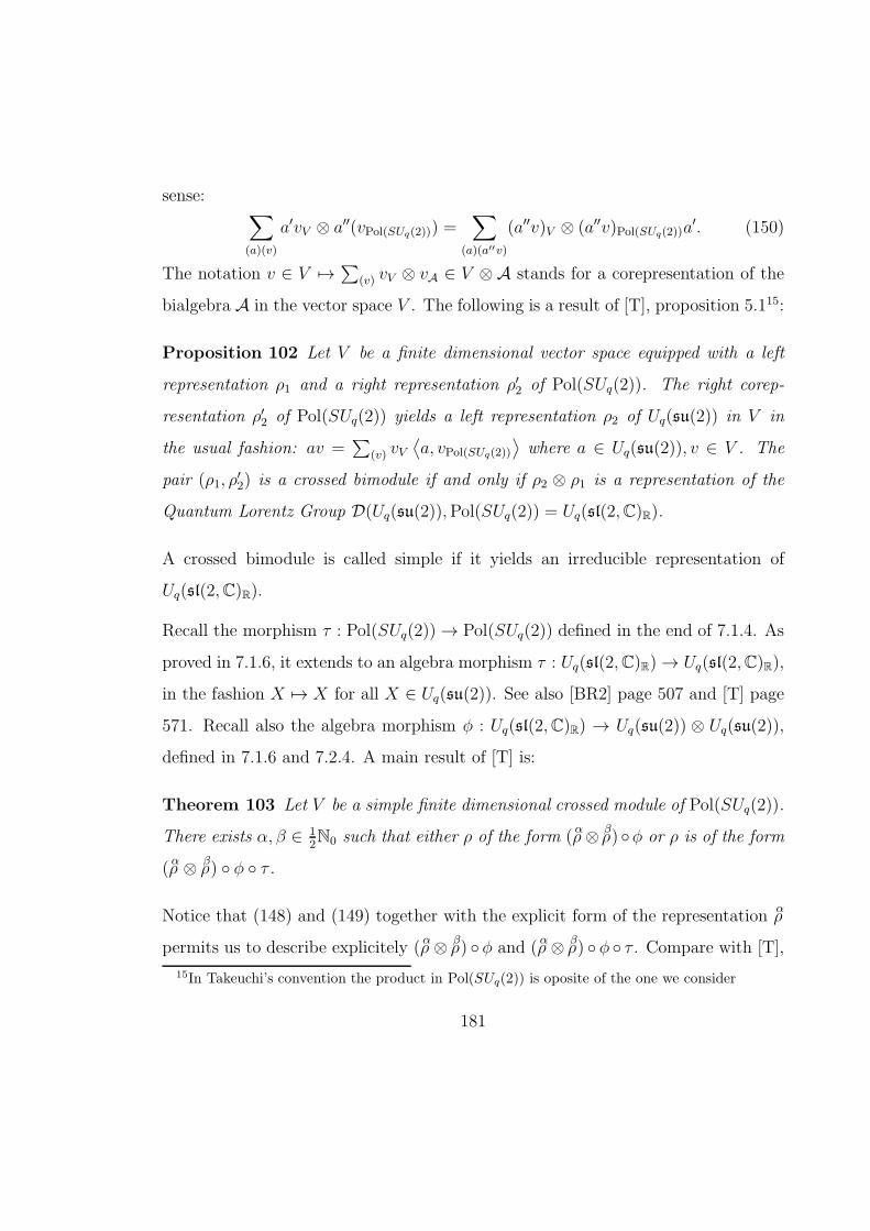
sense:∑
(a)(v)
a′vV ⊗ a′′(vPol(SUq(2))) =∑
(a)(a′′v)
(a′′v)V ⊗ (a′′v)Pol(SUq(2))a′. (150)
The notation v ∈ V 7→∑
(v) vV ⊗ vA ∈ V ⊗ A stands for a corepresentation of the
bialgebra A in the vector space V . The following is a result of [T], proposition 5.115:
Proposition 102 Let V be a finite dimensional vector space equipped with a left
representation ρ1 and a right representation ρ′2 of Pol(SUq(2)). The right corep-
resentation ρ′2 of Pol(SUq(2)) yields a left representation ρ2 of Uq(su(2)) in V in
the usual fashion: av =∑
(v) vV⟨
a, vPol(SUq(2))
⟩
where a ∈ Uq(su(2)), v ∈ V . The
pair (ρ1, ρ′2) is a crossed bimodule if and only if ρ2 ⊗ ρ1 is a representation of the
Quantum Lorentz Group D(Uq(su(2)),Pol(SUq(2)) = Uq(sl(2,C)R).
A crossed bimodule is called simple if it yields an irreducible representation of
Uq(sl(2,C)R).
Recall the morphism τ : Pol(SUq(2)) → Pol(SUq(2)) defined in the end of 7.1.4. As
proved in 7.1.6, it extends to an algebra morphism τ : Uq(sl(2,C)R) → Uq(sl(2,C)R),
in the fashion X 7→ X for all X ∈ Uq(su(2)). See also [BR2] page 507 and [T] page
571. Recall also the algebra morphism φ : Uq(sl(2,C)R) → Uq(su(2)) ⊗ Uq(su(2)),
defined in 7.1.6 and 7.2.4. A main result of [T] is:
Theorem 103 Let V be a simple finite dimensional crossed module of Pol(SUq(2)).
There exists α, β ∈ 12N0 such that either ρ of the form (ρ
α⊗ρβ) φ or ρ is of the form
(ρα⊗ ρ
β) φ τ .
Notice that (148) and (149) together with the explicit form of the representation ρα
permits us to describe explicitely (ρα⊗ ρ
β) φ and (ρ
α⊗ ρβ) φ τ . Compare with [T],
15In Takeuchi’s convention the product in Pol(SUq(2)) is oposite of the one we consider
181

equation (6.4). See also [BR2] page 507.
Notice that not all representations of Uq(su(2)) are dual to corepresentations of
Pol(SUq(2)). This happens if, and only if, they are direct sums of representations
ραwith a ∈ 1
2N0. Therefore Theorem 103 classifies all finite dimensional irreducible
representations of Uq(sl(2,C)R) which, when restricted to Uq(su(2)), are a direct
sum of representations ρα, α ∈ 1
2N0. These representations are the ones which are
dual to corepresentation of the algebra of function in the Quantum Lorentz Group,
in other words the quantum group SLq(2,C) of [PW].
Definition 104 These kind of representations of Uq(sl(2,C)R) are called physical16
representations of D = Uq(sl(2,C)R).
Definition 105 Any finite dimensional representation of Uq(sl(2,C)R) generates a
finite dimensional representation of Uq(su(2)) through the embedding Uq(su(2)) ⊂Uq(sl(2,C)R), therefore any finite dimensional representation ρ of Uq(sl(2,C)R) de-
composes as a direct sum of ραwα’s with each a in 1
2N0 and each wα ∈ 1,−1, i,−i,
uniquely. In addition, if the representation is physical then we always have wα = 1
for any α. The smallest of these α’s is by definition the minimal spin of ρ. The
maximal spin of ρ is the maximum of those.
From the fact φ(X) = φ(X) τ = ∆(X) for any X ∈ Uq(su(2)) and Theorem 103 it
is immediate that
Theorem 106 For any α in 12N0 and the minimal spin of (ρ
α⊗ρα)φ and (ρα⊗ρα)φτ ,
is zero. Moreover, any irreducible physical representation ρ of Uq(sl(2,C)R) with
minimal spin zero is of this form, in fact α is half the maximal spin of ρ.
16This is my nomenclature
182

7.3.2 An equation producing representations
We now give a general form of representations of the Quantum Lorentz Group. Let
D = D(Uq(su(2)),Pol(SUq(2))cop) = Uq(sl(2,C)R) be the Quantum Lorentz Group
at q ∈ (0, 1). Recall equation (137) expressing the product law in the quantum
double. Let a = a ⊗ 1 ∈ D and f = 1 ⊗ f ∈ D, where a ∈ Uq(su(2)) and
f ∈ Pol(SUq(2)). We thus have af = a⊗ f, a ∈ Uq(su(2)), f ∈ Pol(SUq(2)). Let us
consider representations ρ of D of the vector space
V =⊕
α∈N0
Vα
,
where
ρα: Uq(su(2)) → L(V
α
)
is the irreducible representation of Uq(su(2)) with spin α. Compare with 2.1.1.
Notice we are only considering integer spins. The case in which we admit any spins
is similar. It is natural to consider representations in V since through the embedding
Uq(su(2)) → Uq(sl(2,C)R) any finite dimensional representation of Uq(sl(2,C)R)
decomposes as direct sums of representations ραwhen restricted to Uq(su(2)). We
obvioulsy suppose that any element x of Uq(su(2)) acts in V in the fashion:
ρ(x) =∏
α∈N0
ρα(x). (151)
A basis of Vα
is given by the vectors uαi, i = −α,−α + 1, ..., α. Consider an action
of D in V such that Pol(SUq(2)) acts as
gαiαjαvβiβ =
Fβ
Fγ
∑
D,γ ∈N0
∑
−γ≤iγ≤γ−D≤x≤D
vγiγ
iγ iα
γ α
D
x
x
D
α β
jα iβ
ΛαDγβ . (152)
183

The compatibility rules for the spins ensure it is a finite sum and that φ(f)V ⊂ V if
f ∈ Pol(SUq(2)). Extend it to all D as ρ(a⊗ f) = ρ(a)ρ(f). Let us describe which
constraints the constants Λβγαδ need to satisfy. It is obvious that ρ(a)ρ(b) = ρ(ab) if
a ∈ Uq(su(2)) and b ∈ D. One can also show that automatically we have ρ(fa) =
ρ(f)ρ(a) if f ∈ Pol(SUq(2)) and a ∈ Uq(su(2)). This calculation appears in [BR2],
inside the proof of theorem 3. Therefore the only restriction put in the constants
ΛBCAD is that (152) define a representation of Pol(SUq(2)).
The following is a result of [BR2]:
Theorem 107 If
∑
E
A E
B U
C
D
ΛACFEΛBDEP =
∑
K
F A
B U
C
K
A B
P U
K
D
ΛKUFP , (153)
then (151) and (152) define a representation of the Quantum Lorentz Group Uq(sl(2,C)R).
A proof of this is not too difficult, but requires some additional notation and cal-
culations, so will be omitted. The reader can find it in [BR2] inside the proof of
theorem 3. All this is to be compared with 2.1.1 and especially (7).
One observation in need concerns the constants Fα, a ∈ N. Their values are (almost)
arbitrary and they only appear to make some of the representations unitary. In
fact their appearance does not change the representation apart from isomorphism
therefore not affecting the future calculation of knot invariants.
184

7.3.3 A solution of (153) and balanced representations of the Quantum
Lorentz Group
In [BR2], Buffenoir and Roche describe a solution of (153) for any p ∈ C. This ΛBCAD-
coefficients are defined out of a complicated complex continuation of 6j-symbols,
but in a way we can easily prove that the constraints (153) are satisfied. At the end
they are proved to be equal to:
ΛBCAD(p) =∑
σ
0
A
C B
σ −σ
q2σp
−σ σ
B C
D
0
. (154)
We need to choose a logarithm of q, so the best notation would be to consider
q = exp(h). However for q ∈ (0, 1) we have no big ambiguity. We always pick h < 0,
in accordance with before. For completeness, and because this is not show directly
in [BR2] we prove that the coefficients ΛBCAD verify (153), for any p ∈ C. Our main
results depend on this fact, ultimately. The proof goes as:
∑
E
A E
B U
C
D
ΛACFEΛBDEP
=∑
E
A E
B U
C
D
∑
a,b
q2(a+b)p
0
F
C A
a −a
−a a
A C
E
0
0
E
D B
b −b
−b b
B D
P
0
=∑
E
A E
B U
C
D
∑
a,b
q2(a+b)p
0
F
C A
a −a
b −bD B
E
0
0
E
A C
−a a
−b b
B D
P
0
.
185
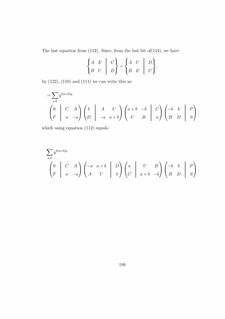
The last equation from (112). Since, from the last bit of(124), we have
A E
B U
C
D
=
A U
B E
D
C
,
by (122), (110) and (111) we can write this as:
=∑
a,b
q2(a+b)p
0
F
C A
a −a
b
D
A U
−a a+ b
a+ b −bU B
C
a
−b b
B D
P
0
,
which using equation (112) equals:
∑
a,b
q2(a+b)p
0
F
C A
a −a
−a a+ b
A U
D
b
a
C
U B
a+ b −b
−b b
B D
P
0
.
186

This term can be written as, again by (122), (110) and (111) :
∑
a,b
q2(a+b)p∑
M,N
C A
U M
F
D
U B
D N
C
P
0 a + b
F U
M
a+ b
a + b
M
C D
a b
a b
C D
N
a + b
a+ b
N
U P
a + b 0
=∑
c
q2cp∑
a+b=c
∑
M,N
C A
U M
F
D
U B
D N
C
P
0 c
F U
M
c
c
M
C D
a b
a b
C D
N
c
c
N
U P
c 0
=∑
c
q2cp∑
M
C A
U M
F
D
U B
D M
C
P
0 c
F U
M
c
c
M
U P
c 0
Y (M,C,D)Y (c,M),
the last step by (116). Therefore by (120) we have:
∑
E
A E
B U
C
D
ΛACFEΛBDEP
=∑
c
q2cp∑
M
C A
U M
F
D
U B
D M
C
P
0 c
F U
M
c
c
M
U P
c 0
.
187

On the other hand we have:
∑
K
F A
B U
C
K
A B
P U
K
D
ΛKUFP
=∑
K
F A
B U
C
K
A B
P U
K
D
∑
c
q2pc
0
F
U K
c −c
−c c
K U
P
0
=∑
K,M
F A
B U
C
K
A B
P U
K
D
U K
U M
F
P
∑
c
q2pc
0 c
F U
M
c
c
M
U P
c 0
. (155)
The last step follow from by (122), (110) and (111). Now, from (124) and (126) we
have:
∑
K
F A
B U
C
K
A B
P U
K
D
U K
U M
F
P
=∑
K
A B
P U
K
D
A B
U F
K
C
U K
U M
F
P
=
U B
D M
C
P
A C
M U
F
D
=
C A
U M
F
D
U B
D M
C
P
,
Which finishes the proof.
Definition 108 (Balanced Representations of the Quantum Lorentz Group)
We have for any p ∈ C a representation ρ(p) of the quantum Lorentz group in V (p).
188
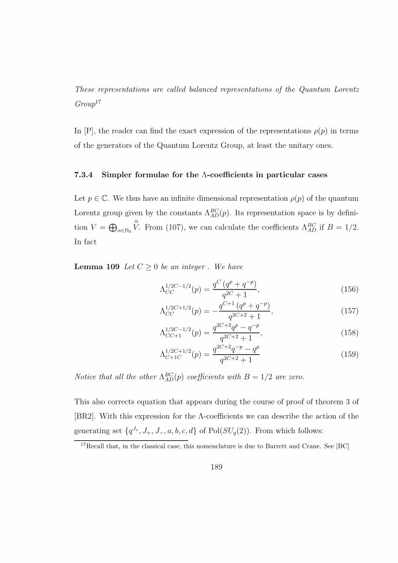
These representations are called balanced representations of the Quantum Lorentz
Group17
In [P], the reader can find the exact expression of the representations ρ(p) in terms
of the generators of the Quantum Lorentz Group, at least the unitary ones.
7.3.4 Simpler formulae for the Λ-coefficients in particular cases
Let p ∈ C. We thus have an infinite dimensional representation ρ(p) of the quantum
Lorentz group given by the constants ΛBCAD(p). Its representation space is by defini-
tion V =⊕
α∈N0Vα
. From (107), we can calculate the coefficients ΛBCAD if B = 1/2.
In fact
Lemma 109 Let C ≥ 0 be an integer . We have
Λ1/2C−1/2CC (p) =
qC (qp + q−p)
q2C + 1, (156)
Λ1/2C+1/2CC (p) = −q
C+1 (qp + q−p)
q2C+2 + 1, (157)
Λ1/2C−1/2CC+1 (p) =
q2C+2qp − q−p
q2C+2 + 1, (158)
Λ1/2C+1/2C+1C (p) =
q2C+2q−p − qp
q2C+2 + 1(159)
Notice that all the other ΛBCAD(p) coefficients with B = 1/2 are zero.
This also corrects equation that appears during the course of proof of theorem 3 of
[BR2]. With this expression for the Λ-coefficients we can describe the action of the
generating set qJz , J+, J−, a, b, c, d of Pol(SUq(2)). From which follows:
17Recall that, in the classical case, this nomenclature is due to Barrett and Crane. See [BC]
189

Theorem 110 Suppose q = exp(h/2). The representations ρ(p) and r(p + 4πih)
are equivalent.
Let us prove the formula for Λ1/2C−1/2CC−1 (p) since the main results we are going to
prove depend on it, ultimately. We have:
1/2 −1/2
C + 1/2 1/2
C + 1
0
−1/2 1/2
1/2 C + 1/2
C
0
= q−(C+1)2
√
[2C + 3][2C + 1][0]![1]![C]![1]![1]![C]![C + 1]![C]![C + 1]![C]!
[1]![2C]![2C + 1]![0]![2C + 3]![2C + 2]![C + 1]![1]![0]![C + 1]!
∑
V,W
qV (C+2)qW (C+1)(−1)V+C(−1)W+1[C + 1 + V ]![W ]![C + 1− V ]![2C + 1−W ]!
[V ]![W ]![C + 1− V ]![C −W ]![C − V ]![1 −W ]![−C + V ]![W ]!.
This last sum is to be extended to all V ’s and W ’s that make the terms inside the
q-factorials positive, thus V = C and W = 0 or W = 1. This last expression thus
simplifies to:
q−(C+1)2 [C]!2
[2C + 2]![2C]!
qC(C+2)[2C + 1]!
[C]!
(
− [2C + 1]!
[C]!+ qC+1 [2C]!
[C − 1]!
)
= q−11
[2C + 2]
(
−[2C + 1] + qC+1[C])
=1
[2C + 2](q − q−1)
(
q−(2C+2) − 1))
= − q−2C−2
1 + q−2C−2= − 1
q2C+2 + 1.
Whereas:
190

−1/2 1/2
C + 1/2 1/2
C + 1
0
1/2 −1/2
1/2 C + 1/2
C
0
= q(C+1)2
√
[2C + 3][2C + 1][0]![1]![C + 1]![1]![0]![C + 1]![C + 1]![C]![C + 1]![C]!
[1]![2C]![2C + 1]![0]![2C + 3]![2C + 2]![C]![1]![0]![C]!
∑
V,W
qV (C+2)qW (C+1)(−1)V+C+1(−1)W [C + V ]![1 +W ]![C + 2− V ]![2C −W ]!
[V ]![W ]![C + 1− V ]![C −W ]![C + 1− V ]![−W ]![−C − 1 + V ]![1 +W ]!,
thus W = 0 and V = C + 1. Therefore this last expression simplifies as:
q−(C+1)2 [C + 1]!2
[2C + 2]![2C]!q(C+1)(C+2) [2C + 1]![2C]!
[C + 1]![C]!= qC+1 [C + 1]
[2C + 2]=
q2C+2
1 + q2C+2.
Notice a strange fact which can be seen from the just obtained expressions for the
Λ-coefficients: The off diagonal terms are zero if q = 1. This is actually immediate
from (154). Comparing with 2.1.1, it appears that the representations ρ(p) do not
have the right limit. A solution for the mystery is obvious from equation (140).
7.3.5 Reapearence of finite dimensional representations
This material seems to be new. Recall the balanced representations ρ(p), p ∈ C
of the Quantum Lorentz defined by (151), (152) and (154). This general form of
representations of the Quantum Lorentz Group contains some finite dimensional
representations. In fact, we have this consequence of Lemma 109:
Proposition 111 Suppose p ∈ N then ρ(p) has a finite dimensional subrepresenta-
tion ρ(p)fin in V (p)fin = 0V ⊕ ...⊕ C
V where C = p− 1.
Compare with 2.2.1.
191
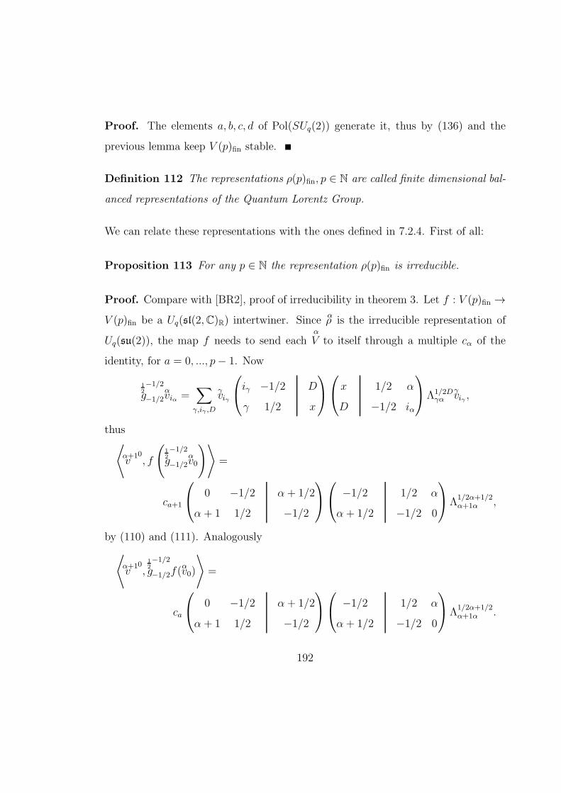
Proof. The elements a, b, c, d of Pol(SUq(2)) generate it, thus by (136) and the
previous lemma keep V (p)fin stable.
Definition 112 The representations ρ(p)fin, p ∈ N are called finite dimensional bal-
anced representations of the Quantum Lorentz Group.
We can relate these representations with the ones defined in 7.2.4. First of all:
Proposition 113 For any p ∈ N the representation ρ(p)fin is irreducible.
Proof. Compare with [BR2], proof of irreducibility in theorem 3. Let f : V (p)fin →V (p)fin be a Uq(sl(2,C)R) intertwiner. Since ρ
αis the irreducible representation of
Uq(su(2)), the map f needs to send each Vα
to itself through a multiple cα of the
identity, for a = 0, ..., p− 1. Now
g12−1/2
−1/2vαiα =
∑
γ,iγ ,D
vγiγ
iγ −1/2
γ 1/2
D
x
x
D
1/2 α
−1/2 iα
Λ1/2Dγα v
γiγ ,
thus⟨
vα+10
, f
(
g12−1/2
−1/2vα0
)⟩
=
ca+1
0 −1/2
α + 1 1/2
α + 1/2
−1/2
−1/2
α + 1/2
1/2 α
−1/2 0
Λ1/2α+1/2α+1α ,
by (110) and (111). Analogously
⟨
vα+10
, g12−1/2
−1/2f(vα0)
⟩
=
ca
0 −1/2
α + 1 1/2
α + 1/2
−1/2
−1/2
α + 1/2
1/2 α
−1/2 0
Λ1/2α+1/2α+1α .
192

Using (107), one sees that the Clebsch-Gordan coefficients in the last two formulae
are not zero if q ∈ (0, 1). Indeed, since q is not a root of unity [n]q! 6= 0 for any
n ∈ N, thus we just need to analyse the terms under the sum in (107). This term
for the coefficient
0 −1/2
α + 1 1/2
α + 1/2
−1/2
simplifies as:
∑
V
qV (C+1)(−1)V[C + 1 + V ]![C + 1− V ]!]
[V ]![C + 1− V ]![C + 1− V ]![−C + V ]!
= q(C+1)C(−1)C(
[2C + 1]!
[C]!− [2C + 2]!
[C + 1]!qC+1
)
= qC[2C + 1]!
[C]!q2C+2.
Notice in the first sum we must have V = C or V = C + 1. The term under the
sum of
−1/2
α+ 1/2
1/2 α
−1/2 0
in (107) simplifies as:
∑
V
qV (C+1)(−1)V[V ]![2C + 1− V ]!
[V ]![C + 1− V ]![1− V ]![−1 + V ]!= −qC+1 [2C]!
[C]!.
None of these terms are zero for q ∈ (0, 1). Thus from the explicit formulae for
Λ1/2α+1/2α+1α , one proves ca = ca+1 for a = 0, ..., p− 2.
The representations ρ(p)fin are physical representations for any p ∈ N, cf. Definition
104. Therefore Theorem 106 can be used. It tells us that either ρ(p) = (ρα⊗ ρ
α) φ
or ρ(p) = (ρα⊗ ρ
α) φ τ , where a = p−1
2. Let us see which one of these ρ(p) is.
Let f : Vfin(p) → Vα
⊗Vα
be an equivalence of representations of the Quantum Lorentz
Group. The representation ρ(p)fin acts on the vector space V pfin = 0
V ⊕ ...⊕ p−1V , and
Uq(su(2)) ⊂ Uq(sl(2,C)R) acts in it as 0ρ ⊕ ... ⊕ p−1
ρ . When restricted to Uq(su(2))
the morphism φ : Uq(su(2)) → Uq(su(2))⊗Uq(su(2)) is simply the comultiplication
in Uq(su(2)), and similarly with φ τ . Therefore, as representations of Uq(su(2)),
193

both (ρα ⊗ ρ
α) φ and (ρ
α ⊗ ρα) φ τ split as 0
ρ ⊕ ... ⊕ p−1ρ . Choose an identification
Vα
⊗ Vα ∼= 0
V ⊕ ... ⊕ p−1V given by the Clebsch-Gordan maps and the phases we have
chosen from them. There must exist constants cβ such that
fV
β = cβidV
β, β = 0, ..., p
These constants are not zero since f is an isomorphism. Recall that a = g12− 1
2
− 12, see
7.1.4. Therefore from (152), (108) and (109)
⟨
v00, av
00
⟩
= Λ12
12
00 . (160)
Thus⟨
v00, f(av
00)⟩
= c0Λ12
12
00 = −c0qp + q−p
q + q−1
On the other hand we know φ(a) = qJz ⊗ q−Jz. Therefore by definition of the
representation ρα⊗ ρ
αand Clebsch-Gordan Coefficients we have:
⟨
v00, φ(a)v
00
⟩
=
⟨
v00,∑
i
0
0
α α
i −i
(
qJz ⊗ q−Jz)
vαi ⊗ v
α−i
i −iα a
0
0
⟩
=∑
−α≤i≤α
0
0
α α
i −i
i −iα a
0
0
q2i
=∑
−α≤i≤α
1
da(−1)2α(−1)−2iq4i, by (118) and (112)
=qp + q−p
q + q−1
For the last step, notice 2α and 2i must have the same parity. Therefore
⟨
v00, φ(a)f(v
00)⟩
= c0qp + q−p
q + q−1
194

Since c0 6= 0, comparing with (101) we conclude we must have ρ(p)fin = (ρα⊗ρα)φτ ,
since τ(a) = −a. We have proved:
Theorem 114 Let p ∈ N. The representation ρ(p)fin is equivalent to (ρα⊗ρα)φ τ ,
where α = p−12.
This re-appearence of finite dimensional representations is also obvious from the
formulae for the unitary representations of the quantum Lorentz Group in [P].
7.3.6 Unitary Balanced Representations
Up to now we have not studied the unitarity of the representations of the Quantum
Lorentz Group. Let us now define a class of unitary representations of Uq(sl(2,C)R),
the unitary balanced representations. They are called simple in [NR].
This discussion is very similar to the one in [BR2], and only is it slightly different
because we use a different definition of ΛBCAD. Consider V =⊕
α∈N0Vα
. It has an
inner product such that vαiα , α ∈ N0,−α ≤ iα ≤ α, since the spin α representation
ραof Uq(su(2)) are unitary, we automatically have < ρ(a)v, w >=< v, ρ(a∗)v >
if v ∈ V and a ∈ Uq(su(2)). Let us find out the conditions so that ρ is also
a unitary representation of Pol(SUq(2)), thus also of D = Uq(sl(2,C)R). Recall
gαiαjα
∗= qjα−iα(−1)iα−jαg
α−iα−jα . We have:
⟨
gαiαjαvβiβ , v
γiγ
⟩
=Fβ
Fγ
∑
M
∑
−M≤y≤M
iγ iα
γ α
M
y
y
M
α β
jα iβ
ΛαMγβ
195
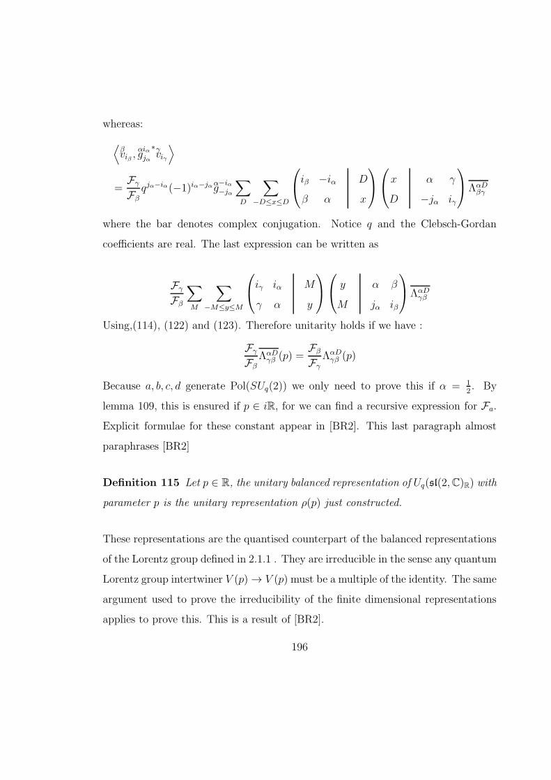
whereas:
⟨
vβiβ , g
αiαjα
∗vγiγ
⟩
=Fγ
Fβqjα−iα(−1)iα−jαg
α−iα−jα
∑
D
∑
−D≤x≤D
iβ −iαβ α
D
x
x
D
α γ
−jα iγ
ΛαDβγ
where the bar denotes complex conjugation. Notice q and the Clebsch-Gordan
coefficients are real. The last expression can be written as
Fγ
Fβ
∑
M
∑
−M≤y≤M
iγ iα
γ α
M
y
y
M
α β
jα iβ
ΛαDγβ
Using,(114), (122) and (123). Therefore unitarity holds if we have :
Fγ
FβΛαDγβ (p) =
Fβ
FγΛαDγβ (p)
Because a, b, c, d generate Pol(SUq(2)) we only need to prove this if α = 12. By
lemma 109, this is ensured if p ∈ iR, for we can find a recursive expression for Fa.
Explicit formulae for these constant appear in [BR2]. This last paragraph almost
paraphrases [BR2]
Definition 115 Let p ∈ R, the unitary balanced representation of Uq(sl(2,C)R) with
parameter p is the unitary representation ρ(p) just constructed.
These representations are the quantised counterpart of the balanced representations
of the Lorentz group defined in 2.1.1 . They are irreducible in the sense any quantum
Lorentz group intertwiner V (p) → V (p) must be a multiple of the identity. The same
argument used to prove the irreducibility of the finite dimensional representations
applies to prove this. This is a result of [BR2].
196

7.3.7 Formal R-matrix and Group Like elements on the Quantum lorentz
Group
We continue to follow [BR2] closely. Let A be a finite dimensional Hopf algebra and
let vi be a basis ofA. Let also vi be the dual basis ofA∗. The quantum double of
A has an R-matrix given by R =∑
i vi⊗1⊗1⊗vi ∈ D(A,A∗cop)⊗D(A,A∗cop). If Ais infinite dimensional, then the expression for R is an infinite sum, however, it may
happen that it makes sense when applied to the tensor product of representations
of A. This is what happens in the quantum Lorentz group case for the balanced
representations ρ(p), p ∈ C and ρ(p)fin, p ∈ N.
Consider the basis gαiαjα of Pol(SUq(2)), where α ∈ 12N0 and −α ≤ iα, jα ≤ α.
When trying to define the dual basis of it in Uq(su(2)), we are led to find elements
zαiαjα ∈ Uq(su(2)) such that
⟨
vβiβ |ρβ(zαiαjα)|v
βjβ
⟩
=⟨
gβiβ
jβ, zαiαjα
⟩
= δ(α, β)δ(iα, jβ)δ(jα, iβ),
whose existence is dubious. The best solution is to modify Uq(su(2)) slightly. For a
vector space V let L(V ) be the algebra of linear maps V → V . Define
Uq(su(2)) =⊕
α∈ 12N0
L(Vα
).
Recall that Uq(su(2)) is embedded in∏
α∈ 12N0L(V
α
) through x 7→∏
α∈ 12N0ρα(x). This
morphism is injective for the elements of Uq(su(2)) are separated by the finite dimen-
sional representations of it. Therefore Uq(su(2)) is almost a subalgebra Uq(su(2)), in
fact it is embedded in its subalgebra of multipliers, cf [BR2]. LetXαiα
jα, α ∈ 12N0,−α ≤
iα, jα ≤ α be the elements of Uq(su(2)) such that Xαiα
jαvβiβ = δ(α, β)δ(iα, iβ)v
αjα. In
particular we have:
Xαiα
jαXβiβ
jβ= X
αiβ
jα, δ(α, β)δ(iα, jβ). (161)
197

There exists an obvious duality between Uq(su(2)) and Pol(SUq(2)) which verifies⟨
Xαiα
jα, gβiβ
jβ
⟩
= δ(α, β)δ(iα, jβ)δ(jα, iβ).
It extends the duality between Uq(su(2)) and Pol(SUq(2)), since⟨
Xαiα
jα, gβiβ
jβ
⟩
=
⟨
vβiβ, Xαiα
jαvβjβ
⟩
= δ(α, β)δ(iα, jβ)⟨
vβiβ, vαjα
⟩
= δ(α, β)δ(iα, jβ)δ(iβ, jα).
We define a coproduct in Uq(su(2)) by dualising the product of Pol(SUq(2)). There-
fore
∆(Xαiα
jα) =∑
β,γ,iβ ,iγ
jβ jγ
β γ
α
jα
iα
α
β γ
iβ iγ
Xβiβ
jβ⊗X
γiγ
jγ .
This infinite sum is interpreted as an element of∏
α,β Vα
⊗ Vβ
. The evaluations (id⊗∆)(X
αiα
jα) and (∆⊗id)(Xαiα
jα) also make sense when interpreted as elements of∏
α,β,γ Vα
⊗Vβ
⊗ Vγ
. The coproduct ∆ is coassociative. The algebra Uq(su(2)) also has a star
structure such that (Xαiα
jα)∗ = X
αjα
iα , thus it is simply matrix transposition. It extends
the star structure in Uq(su(2)), given that the representations ραof Uq(su(2)) in V
α
are unitary.
The expression (137) defining the product quantum double also makes sense when
considering A = Uq(su(2)) and A∗ = Pol(SUq(2)), see [BR2]. We therefore define
D = D(Uq(su(2)),Pol(SUq(2))), thus D is an associative algebra. It also has a star
structure such that
(Xαiα
jα ⊗ gβiβ
jβ)∗ = (X
αiα
jα)∗ ⊗ (g
βiβ
jβ)∗ = X
αjα
iα ⊗ S(gβiβ
jβ).
This last antipode is taken in Pol(SUq(2)).
As pointed out in [BR2], each balanced representation ρ(p) of D gives rise to a
balanced representation ρ(p) of D. This extension is quite natural. The represen-
tation space of ρ(p) is V =⊕
α∈N0. Put X
αiα
jα = Xαiα
jα ⊗ 1 and gαiαjα = 1 ⊗ g
αiαjα. The
198

elements gαiαjα act in V as before, namely as in (152). Recall that if a ∈ Uq(su(2))
then ρ(a) =∏
α∈N0ρα(a) if a ∈ Uq(su(2)). It is thus natural to define
ρ(Xαiα
jα)vβiβ = δ(α, b)δ(iα, iβ)v
αjα. (162)
As proved in [BR2] this action does define a representation of D. This representation
is still unitary for p ∈ iR. For the case p ∈ N we still have a subrepresentation ρ(p)fin
of D. See 7.3.5
The formal R-matrix R in the Quantum Lorentz Group is the infinite sum
R =∑
α,iα,jα
Xαiα
jα ⊗ gαjαiα . (163)
It is easy to see how it acts in the tensor product of two balanced representations
r(p):
Rvαiα ⊗ vβiβ =
∑
D,γ,jα
iγ jα
γ α
D
x
x
D
α β
iα iβ
Fβ
Fγ
ΛαDγβ vαjα ⊗ v
γiγ . (164)
The action of R in V ⊗V is thus well defined, even though R is defined by an infinite
sum. This is a result of [BR1]. Notice we are considering the algebraic, rather than
topological tensor product of vector spaces. Obviously, for the case p ∈ N the action
of R in ρ(p)fin ⊗ ρ(p)fin truncates to the finite sum∑p−1
α=0Xαiα
jα ⊗ gαjαiα .
To determine R−1 we can use the identity (id ⊗ S−1)(R) = R−1 verified by any
R-matrix in a Hopf algebra. We have SD = S−1, where the last antipode is taken in
Pol(SUq(2)) and the first is the one in Uq(sl(2,C)R), see 7.1.4 and 7.1.5. This leads
to the following expression for R−1:
R−1 =∑
α,iα,jα
q−iα+jα(−1)iα−jαXαiα
jα ⊗ gα−iα−jα, (165)
199

which makes sense when applied to the tensor product of two balanced representa-
tions ρ(p).
Obviously, our formal calculations do not prove that R−1 is the inverse of R or that
the action of R in the balanced representations of the Lorentz group defines a braid
group representation. However, we can show this facts directly. For example the
fact RR−1 = id (action in balanced representations) is a consequence of equation
(133), together with the fact ρ(p) is a representation of D if for any representation
ρ(p) of D = Uq(sl(2,C)R). In fact:
RR−1 =∑
α,β,iα,iβ ,jα,jβ
(
Xβiβ
jβ⊗ g
αjβiβ
)(
q−iα+jα(−1)iα−jαXαiα
jα ⊗ gα−iα−jα
)
=∑
a,jα,iα,jβ
q−iα+jα(−1)2α+iα−jαXαiα
jβ⊗ g
αiαjβgα−iα−jα
=∑
a,jα,iα,jβ ,γ,iγ ,jγ
iα −iαα α
γ
iγ
jα
γ
α α
jβ −jα
q−iα+jα(−1)iα−jαXαjα
jβ⊗ g
γiγjγ
=∑
α,jα
Xαiα
iα ⊗ g00
0
this last one acts as the identity in the representations ρ(p). The Yang-Baxter
equation is a consequence of the identities (∆⊗id)(R) = R1,3R1,2 and (id⊗∆)(R) =
R1,3R1,2, when considering the action in the balanced represesentations, see [K] for
example. These last equalities are tautologies when we look at the structure maps
of D.
It is easy to verify that R∗,∗ = R−1, by the very expression of R−1 and the star
structure. Therefore the R-matrix which we consider in the quantum Lorentz Group
is compactible with its star structure, see 7.1.1. Let p ∈ iR, thus ρ(p) is a unitary
200
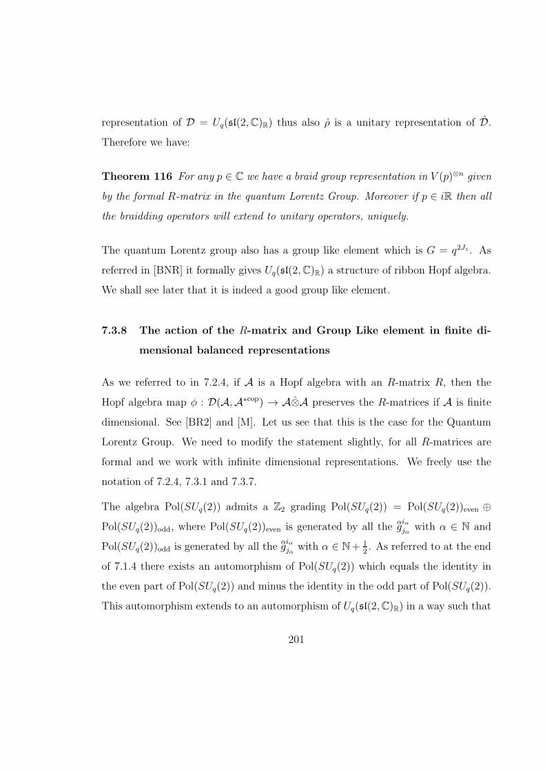
representation of D = Uq(sl(2,C)R) thus also ρ is a unitary representation of D.
Therefore we have:
Theorem 116 For any p ∈ C we have a braid group representation in V (p)⊗n given
by the formal R-matrix in the quantum Lorentz Group. Moreover if p ∈ iR then all
the braidding operators will extend to unitary operators, uniquely.
The quantum Lorentz group also has a group like element which is G = q2Jz . As
referred in [BNR] it formally gives Uq(sl(2,C)R) a structure of ribbon Hopf algebra.
We shall see later that it is indeed a good group like element.
7.3.8 The action of the R-matrix and Group Like element in finite di-
mensional balanced representations
As we referred to in 7.2.4, if A is a Hopf algebra with an R-matrix R, then the
Hopf algebra map φ : D(A,A∗cop) → A⊗A preserves the R-matrices if A is finite
dimensional. See [BR2] and [M]. Let us see that this is the case for the Quantum
Lorentz Group. We need to modify the statement slightly, for all R-matrices are
formal and we work with infinite dimensional representations. We freely use the
notation of 7.2.4, 7.3.1 and 7.3.7.
The algebra Pol(SUq(2)) admits a Z2 grading Pol(SUq(2)) = Pol(SUq(2))even ⊕Pol(SUq(2))odd, where Pol(SUq(2))even is generated by all the g
αiαjα with α ∈ N and
Pol(SUq(2))odd is generated by all the gαiαjα with α ∈ N+ 1
2. As referred to at the end
of 7.1.4 there exists an automorphism of Pol(SUq(2)) which equals the identity in
the even part of Pol(SUq(2)) and minus the identity in the odd part of Pol(SUq(2)).
This automorphism extends to an automorphism of Uq(sl(2,C)R) in a way such that
201

it is the identity in Uq(su(2)) ⊗ 1. As pointed out in 7.3.1 any irreducible physical
representation of Uq(sl(2,C)R) with minimal spin zero is either equivalent to (ρα⊗ρα)
φ or to (ρα⊗ρα)φτ . This is a theorem of Takeuchi, see [T], answering affirmatively
a conjecture formulated Woronowicz and Poddles, see [PW]. In Theorem 114, we
used this result to prove that
ρ(p)fin ∼= (ρα⊗ ρ
α) φ τ, α = (p− 1)/2, p ∈ N.
There exists a map f : V (p)fin → Vα
⊗Vα
intertwining ρ(p)fin and (ρα⊗ρα)φ τ . From
the form of the R-matrix R of the Quantum Lorentz Group, it is obvious that the
action of R is the same in tensor products of representations of the form ρ(p)fin and
of ρ(p)fin τ . Notice again that we are only considering integer spins, thus we only
need the “even part” of the formal R-matrix R. We will use this fact later.
Lemma 117 Let f : φ : V (p)fin → Vα
⊗ Vα
be an intertwiner, and R be the R-matrix
of Uq(su(2))⊗Uq(su(2)), we have:
(f ⊗ f)(Rx⊗ y) = R(f ⊗ f)(x⊗ y)
Let us prove this lemma. In the case A is finite dimensional, this is a consequence
of the fact (φ⊗φ)(R) = R, where the first R-matrix is the R-matrix of the quantum
double. This, as referred in 7.2.4, follows from the equalities (∆⊗ id)(R) = R13R23
and (id ⊗ ∆)(R) = R13R23, satisfied by any R-matrix in a Hopf algebra. The
discussion now is very similar to the one used in the proof of Theorem 114.
The morphism φ : D → Uq(su(2))⊗Uq(su(2)) extends to a morphism φ : D →∏
α,β∈ 12N0L(V
α
)⊗ L(Vβ
). Let us prove that for any v ∈ V (p)fin we have
f
(
Xωiω
jωv
)
= φ
(
Xωiω
jω
)
f(v) (166)
202

Notice that Xωiω
jω is not in D = Uq(sl(2,C)R), thus this fact needs proving. First of
all we need to define:
φ(Xωiω
jω) = ∆(Xωiω
jω) =∑
β,γ,iβ ,iγ ,jβ,jγ
jβ jγ
β γ
ω
jω
iω
ω
β γ
iβ iγ
Xβiβ
jβ⊗X
γiγ
jγ
which acts in Vα
⊗ Vα
in the obvious way. That is as
φ(Xωiω
jω) = ∆(Xωiω
jω) =∑
iβ ,iγ ,jb,jg
jβ jγ
α α
ω
jω
iω
ω
α α
iβ iγ
Xαiβ
jβ⊗X
αiγ
jγ
Recall that φτ when restricted to Uq(su(2)) is the comultiplication in it. Therefore,
as a representation of Uq(su(2)) the representation (ρα⊗ρα)φτ of D = Uq(sl(2,C)R)
splits as 0ρ⊕ ...⊕ p−1
ρ . Fix once for all the identification Vα
⊗ Vα ∼= 0
V ⊕ ...⊕ p−1V given
by the Clebsch-Gordan maps Ψααβ and Φβαα in the phases we have chosen for them.
Under this identification φ(Xωiω
jω) acts in Vα
⊗ Vα
as
φ(Xωiω
jω)vβi = δ(ω, β)δ(iω, i)v
βjω (167)
Indeed, we have:
φ(Xωiω
jω)vβi
=∑
ε
Ψααε
∑
iβ ,iγ ,jβ ,jγ
jβ jγ
α α
ω
jω
iω
ω
α α
iβ iγ
Xαiβ
jβ⊗X
αiγ
jγ
Φβαα(vβi)
=∑
ε,iε,iβ ,iγ ,jβ ,jγ
iε
ε
α α
jβ jγ
jβ jγ
α α
ω
jω
iω
ω
α α
iβ iγ
iβ iγ
α α
β
i
vεiε
= δ(iω, i)δ(ω, β)vβjω
The last equality from (116). This proves that equation (167) is correct.
203

We have two representation of Uq(su(2)), one in V (p)fin and the other in Vα
⊗ Vβ
.
Since f is (in particular) a Uq(su(2))-intertwiner there must exist cβ ∈ C such that
f(vβiβ) = cβv
βiβ . In particular we have:
f
(
Xωiω
jωvβiβ
)
= δ(iω, iβ)δ(ω, β)f(vβjβ) = δ(iω, iβ)δ(ω, β)cβv
βjβ = φ(X
ωiω
jω)f(vβiβ),
which proves (166), is correct. Therefore, if β, γ ∈ 0, 1, ..., p− 1, we have
(f ⊗ f)(Rvβiβ ⊗ vγiγ )
= (f ⊗ f)
∑
a∈ 12N0
(Xαiα
jα ⊗ gαjαiα )(
vβiβ ⊗ v
γiγ
)
= (f ⊗ f)
(
∑
a∈N(Xαiα
jα ⊗ gαjαiα )(
vβiβ ⊗ v
γiγ
)
)
= (f ⊗ f)
(
∑
a∈N(−1)2α(X
αiα
jα ⊗ gαjαiα )(
vβiβ ⊗ v
γiγ
)
)
= (f ⊗ f)
(
∑
a∈N(Xαiα
jα ⊗ τ(gαjαiα ))
(
vβiβ ⊗ v
γiγ
)
)
=∑
α∈N(φ⊗ φ)(X
αiα
jα ⊗ gαjαiα )(
f(vβiβ)⊗ f(v
γiγ ))
=∑
α∈N
∑
(
gαjα
iα
)
∆(Xαiα
jα)⊗ (gαjαiα
′′ ⊗ id)(R(+))⊗ (gαjαiα
′ ⊗ id)(R(−))(
f(vβiβ)⊗ f(v
γiγ ))
Thus, similarly to in the finite dimensional case, all follows from (∆ ⊗ id)(R) =
R13R23 and (id ⊗∆)(R) = R13R23. Indeed, after 7.2.2 the calculations in 7.2.3 are
valid when considering the action in finite dimensional representations. Let us see
it is so. Pick up a β, γ, δ, ε ∈ 12N0. Let use see how the term
∑
α∈N
∑
(
gαjα
iα
)
∆(Xαiα
jα)⊗ (gαjαiα
′′ ⊗ id)(R(+))⊗ (gαjαiα
′ ⊗ id)(R(−))
204

acts in Vβ
⊗Vγ
⊗Vδ
⊗Vε
. Recall the notation of 7.2.2. Let r be the r-form of Pol(SUq(2))
and r = ρ−121 . We have: (we omit the ⊗ symbols, unless we really need them, to
simplify the notation)
⟨
vβiβvγiγv
δiδvεiε
∣
∣
∣
∣
∣
∣
∣
∣
∣
∑
α∈N
∑
(
gαjα
iα
)
∆(Xαiα
jα)⊗ (gαjαiα
′′ ⊗ id)(R(+))⊗ (gαjαiα
′ ⊗ id)(R(−))
∣
∣
∣
∣
∣
∣
∣
∣
∣
vβjβvγjγvδjδvεjε
⟩
=
⟨
vβiβvγiγ
∣
∣
∣
∣
∣
∣
∣
∣
∣
∑
α∈N
∑
(
gαjα
iα
)
∆(Xαiα
jα)⟨
(gαjαiα
′′ ⊗ id)(R(+)), gδiδ
jδ
⟩⟨
(gαjαiα
′ ⊗ id)(R(−)), gεiεjε
⟩
∣
∣
∣
∣
∣
∣
∣
∣
∣
vβjβvγjγ
⟩
=
⟨
vβiβvγiγ
∣
∣
∣
∣
∣
∣
∣
∣
∣
∑
α∈N
∑
(
gαjα
iα
)
∆(Xαiα
jα)r(gαjαiα
′′, gδiδ
jδ)r−121 (g
αjαiα
′, gεiεjε)
∣
∣
∣
∣
∣
∣
∣
∣
∣
vβjβvγjγ
⟩
=
⟨
vβiβvγiγ
∣
∣
∣
∣
∣
∑
α∈N∆(X
αiα
jα) r13r12(gαiαjα, g
δiδ
jδ, gεiεjε)
∣
∣
∣
∣
∣
vβiβvγiγ
⟩
=∑
α∈N
⟨
vβiβvγiγ |∆(X
αiα
jα)|vβiβvγiγ
⟩
r13r12(gαiαjα, g
δiδ
jδ, gεiεjε)
Now notice that∑
α∈N
⟨
vβiβvγiγ |∆(X
αiα
jα)|vβiβvγiγ
⟩
gαiαjα = g
βiβ
jβgγiγjγ
205

Thus the last term simplifies as
r13r12(gβiβ
jβgγiγjγ , g
δiδ
jδ, gεiεjε)
=∑
(
gβiβ
jβ
)
,
(
gγiγjγ
)
r(gβiβ
jβ
′gγiγjγ
′, gεiεjε)r(g
βiβ
jβ
′′gγiγjγ
′′, gδiδ
jδ)
=∑
(
gβiβ
jβ
)
,
(
gγiγjγ
)
,
(
gδiδjδ
)
,
(
gεiεjε
)
r(gβiβ
jβ
′, gεiεjε
′)r(g
γiγjγ
′, gεiεjε
′′)r(g
βiβ
jβ
′′, gδiδ
jδ
′)r(g
γiγjγ
′′, gδiδ
jδ
′′)
= r14r24r13r23(gβiβ
jβ, gγiγjγ , g
δiδ
jδ, gεiεjε)
=⟨
vβiβvγiγv
δiδvεiε∣
∣
∣R
(−)14 R
(−)24 R
(+)13 R
(+)23
∣
∣
∣vβiβvγiγvδiδvεiε
⟩
This finishes the proof of the lemma.
The group like element of Uq(sl(2,C)R) was defined as: G = q2Jz , in particular
φ(G) = q2Jz ⊗ q2Jz = G, where G is the group like element of Uq(su(2))⊗Uq(su(2)).Thus in the conditions of the last theorem we also have: f(Gx) = Gf(x). By the
discussion in 7.2.4, the map φ : Uq(sl(2,C)R) → Uq(su(2))⊗Uq(su(2)) also preserves
the comultiplication map and the antipodal map. Since the category of represen-
tations of Uq(su(2))⊗Uq(su(2)) which are direct sums of representations ρα ⊗ ρ
βis a
ribbon category, it follows that:
Theorem 118 . The tensor category of finite dimensional representations of the
quantum Lorentz Group generated by the balanced representations is a ribbon cate-
gory when the Quantum Lorentz Group is given the formal R-matrix R and group
like element G = q2J . It is ribbon equivalent to the subcategory of representations of
Uq(su(2))⊗Uq(su(2)) generated by representations ρα⊗ ρ
α
Therefore we have a knot invariant I(ρ(p)fin) for any finite dimensional balanced
206
representation ρ(p)fin of the quantum Lorentz group made out of the formal R-
matrix and group like elements. Moreover by, Lemma 101, it follows that:
Theorem 119 Let q ∈ (0, 1). Let p ∈ N and 2α = p− 1. We have:
I(ρ(p)fin)(q1/2)(K) = X(0, p,K)(−h)(2α+ 1),
where q = exp(h) and h < 0, for any knot K. In particular these knot invariants
are unframed and do not distinguish a knot from its mirror image.
This proves our perturbative framework in chapter 2 is correct at least for finite
dimensional balanced representations. We will see later that the same holds for
infinite dimensional balanced representations.
7.4 Knot invariants from infinite dimensional representa-
tions of the Quantum Lorentz Group
We now apply the machinery of the last sections to define knot invariants from
infinite dimensional representations of the Quantum Lorentz Group.
7.4.1 Representations of the Quantum Lorentz Group and R-matrix-a
resume of the notation
Recall that the Quantum Lorentz Group D = Uq(sl(2,C)R) at a point q ∈ (0, 1)
is defined as the quantum double D(Uq(su(2)),Pol(SUq(2))cop), notice that both
Uq(su(2)) and Pol(SUq(2))cop are sub Hopf algebras of D. Therefore D has a formal
R-matrix R coming from its quantum double structure. As we have seen in 7.3.7,
207

even though R is defined by an infinite sum, it is possible to describe its action in
any pair of infinite dimensional irreducible balanced representations of D, as well as
in the balanced finite dimensional representations. See 7.3.7
Recall that the balanced representations of Uq(sl(2,C)R) depend on p ∈ C. If p ∈ iR
then the representations ρ(p) can be made unitary. Choosing p ∈ [0, i2πh], where
q = eh, parametrises all the unitary representations in the principal series which
have minimal spin equal to zero. These last ones are called simple representations
in [NR].
Similarly to the classical case, the underlying vector space for the balanced repre-
sentations ρ(p), p ∈ C of the Quantum Lorentz Group is
V = V (p) =⊕
α∈N0
Vα
,
where
ρα: Uq(su(2)) → L(V
α
)
is the irreducible representation of Uq(su(2)) with spin α. A basis of Vα
is thus given
by the vectors uαi, i = −α,−α + 1, ..., α. Any element x of Uq(su(2)) acts in V in
the fashion:∏
α∈N0
ρα(x).
The group like element of the Lorentz group is given by G = q2Jz .
Define, given half integers A,B,C and D, the complex numbers
ΛBCAD(ρ) =∑
σ
0
A
C B
σ −σ
q2σρ
−σ σ
B C
D
0
. (168)
For the correct definition of the phases of the Clebsh-Gordon coefficients see [BR2]
or [KS]. We displayed an expression for them in 7.1.2, a formula taken from [BR2].
208

Recall the formal universal R-matrix of the quantum Lorentz group is: (see [BR1]
and 7.3.7)
R =∑
α∈ 12N0
−α≤ia,ja≤α
Xαiα
jα ⊗ gαjαiα ,
its inverse being:
R−1 =∑
α∈ 12N0
−α≤ia,ja≤α
Xαiα
jα ⊗ S−1(gαjαiα ).
This antipode S is the one of Pol(SUq(2))cop ⊂ D, which is the inverse of the one in
Pol(SUq(2)), thus
S(gαjαiα ) = q−iα+jα(−1)−jα+iαg
α−iα−jα.
See 7.1.4 The action of gαiαjα in the space V (p) is given by
gαiαjαvβiβ =
Fβ
Fγ
∑
D,γ,p,r,x 12N0
vγiγ
iγ iα
γ α
D
x
x
D
α β
jα iβ
ΛαCγβ . (169)
The constants Fα are defined in [BR2], proposition 1. They will not be used di-
rectly. In fact as we refered to in 7.3.3, their values are (almost) arbitrary and they
only appear to ensure that the representations ρ(p) are unitary for p ∈ iR. Their
appearance does not change the representation itself, therefore not affecting the cal-
culations of knot invariants. Notice also that equation (169) implies that g12i
j sends Vγ
to Vγ−1
⊕ Vγ
⊕ Vγ+1
.
In some particular cases, equation (169) simplifies to:
gαiαjαv
00 =
F0
Fγ
∑
γ,iγ
iγ iα
γ α
α
jα
Λααγ0 vγiγ , (170)
and to⟨
v00, gαiαjαvβiβ
⟩
=Fb
F0
iα
α
α β
jα iβ
Λαα0β . (171)
209
All these formulae are consequences of (108) and (109). With them we can also
prove Λ0ααα = 1, from which follows:
g00
0vαiα = v
αiα. (172)
As we saw in 7.3.7, the elements
Xαiα
jα, α ∈ 1
2N0, iα = −α, ..., α
act simply as matrix elements, in other words:
Xαiα
jαvβiβ = δ(α, β)δ(ia, iβ)v
αjα. (173)
The action of the group like element G is
Gvαiα = q2iav
αiα. (174)
It is easy to compute how R acts, namely:
R(
vαiα ⊗ v
βiβ
)
=∑
D,γ,jα
iγ jα
γ α
D
x
x
D
α β
iα iβ
Fβ
FγΛαDγβ
(
vαjα ⊗ v
γiγ
)
.
See [BR1], proposition 13. The action of R in V ⊗V is thus well defined. Notice that
we are considering the algebraic, rather than topological, tensor product. Moreover
R defines a braid group representation. We proved this in 7.3.7. Denote it by
b ∈ B(n) 7→ Rb ∈ L(V ⊗). Here B(n) denotes the n-strand braid group and L(V ⊗n)
the vector space of linear maps V ⊗n → V ⊗n. Notice that the braiding operators
Rb extend to unitary operators if p ∈ iR since R∗⊗∗ = R−1, where ∗ is the star
structure on the Quantum Lorentz Group, see 7.3.7.
210

7.4.2 Some heuristics
Recall 1.4.2 as well now. Suppose we are given a braid b with n + 1 strands, there
is attached to it q braiding operator Rb : V ⊗(n+1) → V ⊗(n+1), for any balanced
representation of the Quantum Lorentz Group. Consider the map Ab = (id ⊗ G ⊗... ⊗ G)Rb. Suppose the closure of the braid b is a knot. If the representations we
are considering were finite dimensional then the partial trace T 1(Ab) : V → V of Ab
over the last n variables would be an intertwiner, and thus a multiple of the identity,
given that the representations which we are considering are irreducible. Moreover
this multiple of the identity would be a knot invariant which would have the form:
b 7→∑
α1,...,an∈N0
⟨
v00 ⊗ v
α1iα1 ⊗ ...⊗ vαniαn , Ab
(
v00 ⊗ v
α1iα1
⊗ ...⊗ vαn
iαn
)⟩
. (175)
The last sum is to be also extended to all iαkwith −αk ≤ iαk
≤ αk, k = 1, ..., n− 1.
Even though the sums above may be not convergent, the assignment of one sum of
this kind to a braid whose closure is a knot is not ambiguous. In fact suppose b has
m+ 1 strands and n crossings. We can always express this sum in a more sugestive
way, namely as:
Sb =∑
a1,...,αn
−αl≤il,jl≤αl
⟨
v00,
2n+m∏
l=1
T (α, i, j, l)v00
⟩
, (176)
where α = (α1, ..., αn), i = (i1, ..., in), j = (j1, ..., jn), and T (α, i, j, l) can be either a
term like gαkij , a term like X
αki
j or G. We obvioulsy need to suppose that the closure of
b is a knot for this to hold. Notice that the transition from (175) to (176) is totaly
clear if the representations are finite dimensional, and corresponds to the approach
in 1.4.2. We wish to analyse the sums b 7→ Sb where b is a braid whose closure is
a knot. We shall see that they do define a knot invariant after we consider their
asymptotic expansion.
211
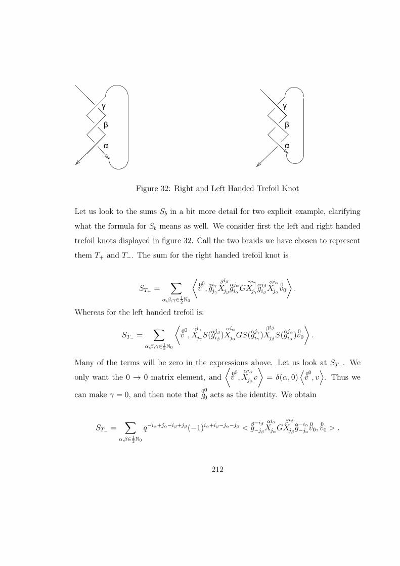
α
β
γ
α
β
γ
Figure 32: Right and Left Handed Trefoil Knot
Let us look to the sums Sb in a bit more detail for two explicit example, clarifying
what the formula for Sb means as well. We consider first the left and right handed
trefoil knots displayed in figure 32. Call the two braids we have chosen to represent
them T+ and T−. The sum for the right handed trefoil knot is
ST+ =∑
α,β,γ∈ 12N0
⟨
v00, gγiγjγX
βiβ
jβgαjαiαGX
γiγ
jγgαjβiβXαiα
jαv00
⟩
.
Whereas for the left handed trefoil is:
ST− =∑
α,β,γ∈ 12N0
⟨
v00, Xγiγ
jγS(gαjβiβ)Xαiα
jαGS(gαjγiγ )X
βiβ
jβS(g
αjαiα )v
00
⟩
.
Many of the terms will be zero in the expressions above. Let us look at ST− . We
only want the 0 → 0 matrix element, and
⟨
v00, Xαiα
jαv
⟩
= δ(α, 0)⟨
v00, v⟩
. Thus we
can make γ = 0, and then note that g00
0 acts as the identity. We obtain
ST− =∑
α,β∈ 12N0
q−iα+jα−iβ+jβ(−1)iα+iβ−jα−jβ < gβ−iβ−jβX
αiα
jαGXβiβ
jβgα−iα−jav
00, v
00 > .
212

From (162) and (174) follows α = β and iα = jβ . By (170) and (171) we can
conclude:
ST− =∑
α∈ 12N0
α∑
iβ ,jβ,jα=−αqjα−iβ+2jβ(−1)iβ−jβ
−iβα
α α
−jβ jα
iβ −jβα α
α
−jα
Λαα0αΛααα0 .
Using the standard symmetries of the Clebsch Gordon Coefficients, namely equation
(114), we can express this as:
ST− =∑
α∈N0
α∑
iβ ,jβ ,jα=−αq2jβ
−iβ −jαα α
α
−jβ
−jβα
α α
−iβ −jα
Λαα0αΛααα0 .
Notice Λααα0 is zero unless α is integer. Therefore the final expression for the sum is:
ST− =∑
α∈N0
dαΛαα0αΛ
ααα0 .
Here da is the quantum dimension of the representation ρα. It equals (q2α+1 −
q−2α−1)/(q − q−1). This last sum is easily proved to be equal to ST+, therefore,
if the sums do define a knot invariant, they make no distinction between the Trefoil
and its mirror image. We would expect this from Corollary 19 and Theorem 119.
The calculations for other knot diagrams follow the same procedure, which can be
given an obvious graphical calculus.
Notice that the series S(T−) seems to be divergent due to the presence of the dα
term in it. Therefore these sums do not seem to define C-valued knot invariants.
We will go back to this in 7.4.5. This tells us the method of Borel re-summation
sketched in Chapter 4 is perhaps more powerful.
213

As we have seen in 7.3.5, if p ∈ N, then the representation ρ(p) has a finite dimen-
sional subrepresentation ρ(p)fin in V (p)fin = 0V⊗ 1
V ⊕...⊕p−1V . Notice that v
00 ∈ V (p)fin.
Therefore from (173) and (176) we have:
Lemma 120 If p ∈ N and b is a braid whose closure is a knot, then the infinite
sum Sb(q, p) truncates to a finite sum for any q ∈ (0, 1).
And by Theorem 119 we must have:
Proposition 121 Let q = exp(h/2) ∈ (0, 1), and p ∈ N. Let also α = (p − 1)/2.
Given a braid b, let Kb be the closure of b, which we suppose to be a knot. We have:
Sb(exp(h/2), p)[2α+ 1]2 = X(0, p,Kb)(−h)(2α + 1)2
where α = (p− 1)/2 and h < 0.
Recall that by theorem 14 the knot invariant X(0, p) is unframed for any p ∈ N.
7.4.3 The series are convergent h-adicaly
We now define a simple version the h-adic version of the theory developed by Buf-
fenoir and Roche18
Let∑
n anhn be a formal power series. The order of it is by definition the smallest n
so that an 6= 0. Let∑
k A(k) =∑
k
(
∑
n a(k)n hn
)
be a series of formal power series.
18Maybe it would have been better to define an h-adic quantum Lorentz group as
D(Uh(sl(2,C)), SLh(2,C)) from the begining. This quantum Group which would then natu-
rally map to Uh(sl(2,C))⊗ Uh(sl(2,C)). This would avoid the technicalities arising from the fact
Uq(su(2)) is not an honest ribbon Hopf algebra. However, we could not, a priory, apply Takeuchi’s
theorem (Theorem 103), a result in which a major part of our work depends.
214
We say it is converges h-adically if for any m ∈ N the number of k’s in N such that
the power series A(k) has order smaller than m is finite. Therefore we can define∑
k
(
∑
n a(k)n hn
)
without any problem.
Let q ∈ (0, 1) and consider the element gαiαjα ∈ Pol(SUq(2)). For any p ∈ C, we have
a balanced representations ρ(p) of the quantum Lorentz group in V (p). The term
⟨
vβiβ |ρ(p)(gαiαjα)|v
γiγ
⟩
q
can be seen a function of q. Due to the fact the building blocks of ρ(p) are Clebsch
Gordon coefficients, it express as a sum of square roots of rational functions of q,
which extend to a well defined analytic function in a neighborhood of 1. We can see
this for example from (107). In addition we have some terms of the form qpσ, σ ∈ Z,
which after putting q = exp(h/2) define an analytic function of h. Therefore
h 7→⟨
vβiβ |ρ(p)(gαiαjα)|v
γiγ
⟩
exp(h/2)
defines a power series in h, uniquely. In particular it follows that if b is a braid whose
closure is a knot, then each term of the sum Sb defines uniquely a power series in h,
which converges to the term for h ≤ 0 close enough to 0 and q close enough to 1.
Lemma 122 For any x ∈ Pol(SUq(2)), the order of
h 7→⟨
vβiβ |ρ(p)(x)|vγiγ
⟩
exp(h/2)
is bigger or equal to |β − γ| as a power series in h.
Proof. Notice that g12i
j sends Vγ
to Vγ−1
⊕ Vγ
⊕ Vγ+1
, in a way such that for q = 1
the projection v of g12i
jvγiγ in V
γ+1
⊕ Vγ−1
is zero. We can see this from Lemma 109, for
example. In particular v has order bigger or equal to one. This lemma is thus a trivial
215
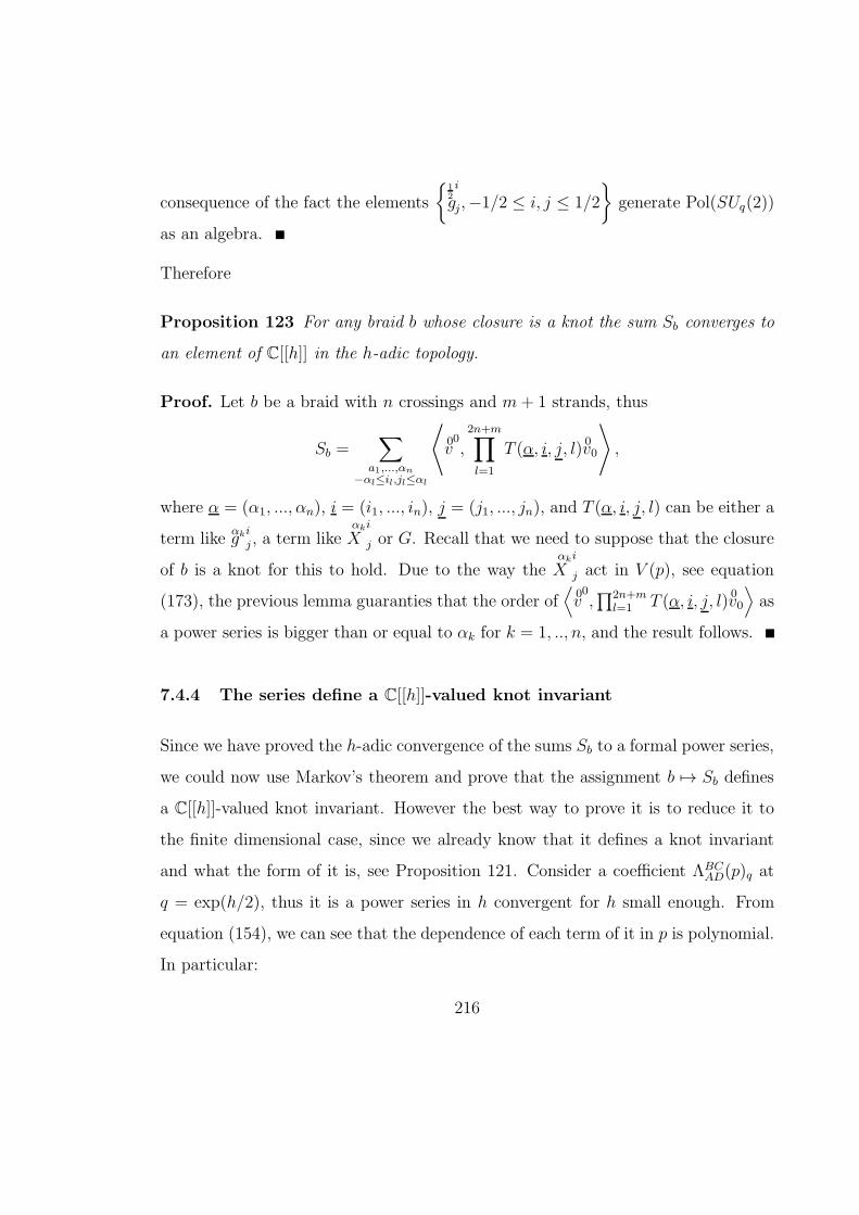
consequence of the fact the elements
g12i
j,−1/2 ≤ i, j ≤ 1/2
generate Pol(SUq(2))
as an algebra.
Therefore
Proposition 123 For any braid b whose closure is a knot the sum Sb converges to
an element of C[[h]] in the h-adic topology.
Proof. Let b be a braid with n crossings and m+ 1 strands, thus
Sb =∑
a1,...,αn
−αl≤il,jl≤αl
⟨
v00,2n+m∏
l=1
T (α, i, j, l)v00
⟩
,
where α = (α1, ..., αn), i = (i1, ..., in), j = (j1, ..., jn), and T (α, i, j, l) can be either a
term like gαkij , a term like X
αki
j or G. Recall that we need to suppose that the closure
of b is a knot for this to hold. Due to the way the Xαki
j act in V (p), see equation
(173), the previous lemma guaranties that the order of⟨
v00,∏2n+m
l=1 T (α, i, j, l)v00
⟩
as
a power series is bigger than or equal to αk for k = 1, .., n, and the result follows.
7.4.4 The series define a C[[h]]-valued knot invariant
Since we have proved the h-adic convergence of the sums Sb to a formal power series,
we could now use Markov’s theorem and prove that the assignment b 7→ Sb defines
a C[[h]]-valued knot invariant. However the best way to prove it is to reduce it to
the finite dimensional case, since we already know that it defines a knot invariant
and what the form of it is, see Proposition 121. Consider a coefficient ΛBCAD(p)q at
q = exp(h/2), thus it is a power series in h convergent for h small enough. From
equation (154), we can see that the dependence of each term of it in p is polynomial.
In particular:
216

Lemma 124 Let b be a braid whose closure is a knot Kb, consider the power series
S(b)(exp(h/2), p) as a function of p, the parameter defining a balanced representa-
tion of the quantum Lorentz Group. Then each term in the expansion of S(b) is a
polynomial in p.
Proof. Cf 3.3.1. Suppose A(p) =∑
n∈N0An(p)h
n and B(p) =∑
n∈N0Bn(p)h
n are
power series whose coefficients depend polynomially in p, for example a power series
such as exp(mph/2). Then also the coefficients of their product depend polynomially
in p. This immediately proves this lemma since the Clebsch-Gordan coefficients do
not depend on p.
Therefore
Theorem 125 Let p ∈ C and b be a braid whose closure is a knot Kb. We have:
Sb(exp(h/2), p)[2a+ 1]2 = X(0, p,Kb)(−h)(2α + 1)2
where α = (p− 1)/2
Recall that by theorem 14 the knot invariant X(0, p) is unframed.
Proof. By Lemma 124, we only need to prove this theorem for p ∈ N. In this case,
if q = (0, 1) then S(p, q) truncates to a finite sum which from Proposition 121 equals
X(0, p,Kb)(−h) (2α+1)2
[2α+1]2at h = exp(h/2). Recall these power series are convergent
if p is integer. Each term of the finite sum S(p, exp(h/2)) is a power series in h
convergent for h small enough and coinciding with S(p, q), for q ∈ (0, 1) and close
enough to 1; thus the result follows.
This theorem totally unifies the approach in chapter 2 and this one in the context
of balanced representations.
217

7.4.5 Estimates for Clebsch Gordon Coefficients and Λ-coefficients, and
the series ST+
We now estimate how fast the series ST+ can diverge, now interpreted as a series of
complex numbers.
First of all we make the observation that the orthogonality relations for the Clebsch
Gordon coefficients imply that they are in norm smaller than one, for they are real
in our convention, which is as usual the one of [BR2], see 7.1.2. We can actually get
a better estimate. First, let us try to find a bound for a Clebsch-Gordan coefficient
of the form
σ −σB C
D
0
. Notice that in general.
0
A
C B
−σ σ
=
−σ σ
C B
A
0
=
−σ σ
B C
A
0
. (177)
See 7.1.2.
We have, see [BR2] and 7.1.2:
σ −σB C
D
0
= qσ+12((C+1)C−(B+1)B−(D+1)D).eiπ(B−σ)
√
[2D + 1][B + C −D]![B − σ]![D]![D]!
[D + C − B]!B +D − C]![B + C +D + 1]![B + σ]![C − σ!
D∑
V=0D−C−σ≤V≤B−σ
QV (D+1)eiπ(V+B−σ)[B + σ + V ]![C +D − σ − V ]!
[V ]![D − V ]![B − σ − V ]![C −D + σ + V ]!.
The quantum integers are defined as [n] = [n]q =q−n−qnq−1−q . As usual we assume q ∈
(0, 1) Note that we can make the substitution [n]q 7→ q−n− qn in the formula above
218
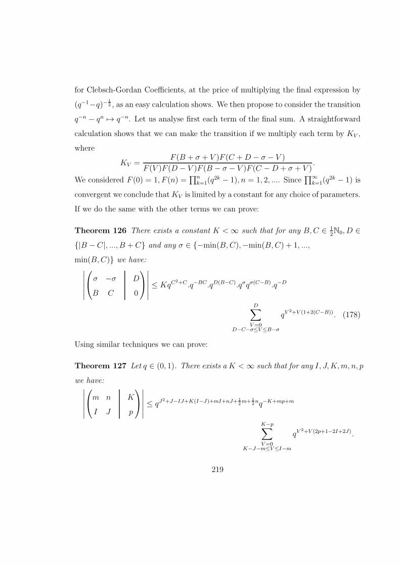
for Clebsch-Gordan Coefficients, at the price of multiplying the final expression by
(q−1−q)− 12 , as an easy calculation shows. We then propose to consider the transition
q−n − qn 7→ q−n. Let us analyse first each term of the final sum. A straightforward
calculation shows that we can make the transition if we multiply each term by KV ,
where
KV =F (B + σ + V )F (C +D − σ − V )
F (V )F (D − V )F (B − σ − V )F (C −D + σ + V ).
We considered F (0) = 1, F (n) =∏n
k=1(q2k − 1), n = 1, 2, .... Since
∏∞k=1(q
2k − 1) is
convergent we conclude thatKV is limited by a constant for any choice of parameters.
If we do the same with the other terms we can prove:
Theorem 126 There exists a constant K <∞ such that for any B,C ∈ 12N0, D ∈
|B − C|, ..., B + C and any σ ∈ −min(B,C),−min(B,C) + 1, ...,
min(B,C) we have:∣
∣
∣
∣
∣
∣
σ −σB C
D
0
∣
∣
∣
∣
∣
∣
≤ KqC2+C .q−BC .qD(B−C).qσqσ(C−B).q−D
D∑
V=0D−C−σ≤V≤B−σ
qV2+V (1+2(C−B)). (178)
Using similar techniques we can prove:
Theorem 127 Let q ∈ (0, 1). There exists a K <∞ such that for any I, J,K,m, n, p
we have:∣
∣
∣
∣
∣
∣
m n
I J
K
p
∣
∣
∣
∣
∣
∣
≤ qJ2+J−IJ+K(I−J)+mI+nJ+ 1
2m+ 1
2nq−K+mp+m
K−p∑
V=0K−J−m≤V≤I−m
qV2+V (2p+1−2I+2J).
219
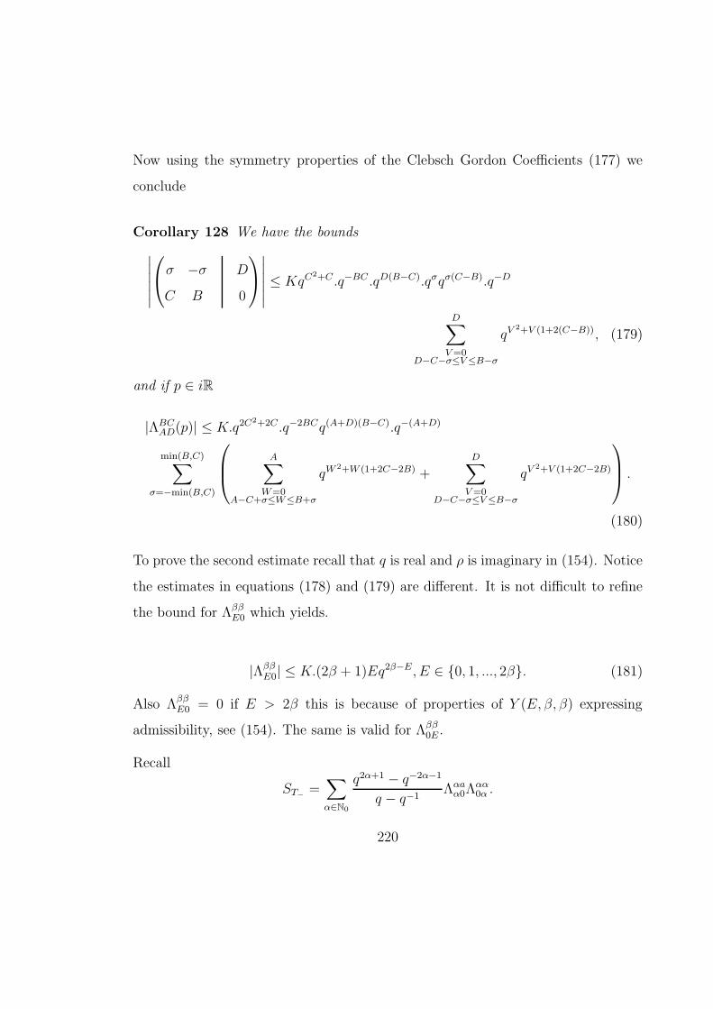
Now using the symmetry properties of the Clebsch Gordon Coefficients (177) we
conclude
Corollary 128 We have the bounds
∣
∣
∣
∣
∣
∣
σ −σC B
D
0
∣
∣
∣
∣
∣
∣
≤ KqC2+C .q−BC .qD(B−C).qσqσ(C−B).q−D
D∑
V=0D−C−σ≤V≤B−σ
qV2+V (1+2(C−B)), (179)
and if p ∈ iR
|ΛBCAD(p)| ≤ K.q2C2+2C .q−2BCq(A+D)(B−C).q−(A+D)
min(B,C)∑
σ=−min(B,C)
A∑
W=0A−C+σ≤W≤B+σ
qW2+W (1+2C−2B) +
D∑
V=0D−C−σ≤V≤B−σ
qV2+V (1+2C−2B)
.
(180)
To prove the second estimate recall that q is real and ρ is imaginary in (154). Notice
the estimates in equations (178) and (179) are different. It is not difficult to refine
the bound for ΛββE0 which yields.
|ΛββE0| ≤ K.(2β + 1)Eq2β−E, E ∈ 0, 1, ..., 2β. (181)
Also ΛββE0 = 0 if E > 2β this is because of properties of Y (E, β, β) expressing
admissibility, see (154). The same is valid for Λββ0E .
Recall
ST− =∑
α∈N0
q2α+1 − q−2α−1
q − q−1Λαaα0Λ
αα0α .
220

Therefore if p ∈ iR the series diverges at most as19:
∑
α∈N(2α + 1).
References
[AC] Altschuler D., Coste A., Quasi-Quantum Groups, Knots, Three Manifolds
and Topological Field Theory; Commun. Math. Phys., 150,83-107 (1992)
[AF] Altschuler, D., Freidel, L.: On universal Vassiliev Invariants, XIth Interna-
tional Congress of Mathematical Physics (Paris, 1994), 709–710, Internat.
Press, Cambridge, MA, 1995.
[BC] Barrett J.W., Crane L.: A Lorentzian Signature Model for Quantum Gen-
eral Relativity, Class. Quant. Grav. 17 (2000) 3101-3118
[BR1] Buffenoir E., Roche Ph: Tensor Product of Principal Unitary Representa-
tions of Quantum Lorentz Group and Askey-Wilson Polynomials , Journal
of Mathematical Physics 41 (11), 7715-7751, Nov 2000
[BR2] Buffenoir E., Roche Ph., Harmonic Analysis in the Quantum Lorentz Group,
Commun. Math. Phys., 207 (3), 499-555 ( 1999)
[BN] Bar-Natan D.: On the Vassiliev Knot Invariants, Topology Vol. 34 No. 2
(1995) pp 423-472.
19Numerical calculation with maple sugest that the series ST+is indeed divergent and that this
is the exact divergence rate
221

[BNR] Buffenoir,E., Noui, K., Roche, Ph.: Hamiltonian Quantisation of Chern
Simons Theory with SL(2,C) group, Class. Quant. Grav. 19 (2002) 4953-
5015, hep-th/0202121
[C] Chmutov S.: A Proof of the Melvin Morton Conjecture and Feynmann
Diagrams, J. Knot Theory Ramif (7) 1, 23-40, Feb 1998
[CD] Chmutov S., Duzhin S.: The Kontsevich Integral, Acta. Appl. Math 66 (2)
155-190, April 2001
[CH] Chabat B.: Introducion a l’analyse complexe , Tome 1, Editions Mir, 1990
[CP] Chari V, Pressley A: A Guide to Quantum Groups, Cambridge University
press 1994
[CV] Chmutov S, Varchenko A., Remarks on The Vassiliev Invariants coming
from sl2, Topology, Vol 36, No. 1, pp 153-178, 1997
[D1] Drinfeld V. G.: Quasi Hopf Algebras, Leningrad Math. J. 1 (1990) 1419-
1457
[D2] Drinfeld V. G: on Quasi Triangular Quasi Hopf Algebras and a Group
Closelly related with Gal(Q/Q), Leningrad Math. J. 2 (1991) 829-860
[FL] Freidel L., Louapre D.: Non-perturbative summation over 3D discrete
topologies, hep-th/0211026
[FM1] Faria Martins, J: On the Analytic Properties of the z-coloured Jones Poly-
nomial, To appear in Journal of Knot Theory and its ramifications
[FM2] Faria Martins, J:Knot Theory with the Lorentz Group, mathQA/
222
[FY] Freyd P., Yetter D.: Coherence theorems via knot theory. J. Pure Appl.
Algebra 78 (1992), no. 1, 49–76.
[G] Gukov,S: Three-Dimensional Quantum Gravity, Chern-Simons Theory, and
the A-Polynomial, hep-th/0306165
[GI] Garcia-Islas M.: (2 + 1)-dimensional quantum gravity, spin networks and
asymptotics, Classical Quantum Gravity 21 (2004), no. 2, 445–464
[GMS] Gel’fand I. M., Minlos R.A., Shapiro Z.Ya.: Representations of the Rotation
and Lorentz groups and their Applications, Oxford Pergamon, 1963
[GGV] Gel’fand I. M., Graev M. I., Vilenkin N. Ya.:Generalized Functions, volume
5, Integral geometry and representation Theory, Academic Press 1966
[GN] Garoufalidis S, Bar-Natan D: On the Melvin-Morton-Rozansky Conjecture
Inventiones Mathematicae 125 (1996) pp 103-133
[H] Habiro, K.: On the quantum sl2 invariants of knots and integral homology
spheres. Invariants of knots and 3-manifolds (Kyoto, 2001), 55–68 (elec-
tronic), Geom. Topol. Monogr., 4, Geom. Topol. Publ., Coventry, 2002.
[K] Kassel C. : Quantum Groups, Springer-Werlag 1994
[Kir] Kirillov A. A.: Elements of the Theory of Representations, Springer-Verlag,
1976.
[Ko] Kontsevich M: Vassiliev’s knot invariants. I. M. Gel’fand Seminar, 137–150,
Adv. Soviet Math., 16, Part 2, Amer. Math. Soc., Providence, RI, 1993.
223

[KS] Klimyk A., Schmudgen K.: Quantum Groups and their representations,
Springer, 1997
[KT] Kashaev R.M., Tirkkonen O.: A Proof of the Volume Conjecture for Torus
Knots, J. Math. Sci. (New York) 115 (2003), no. 1, 2033 -2036
[L] Lang S.: SL(2;R), Addison-Wesley, Reading, MA, 1975
[LM1] Le TQ, Murakami J., The Universal Vassiliev-Kontsevitch Invariant for
Framed Oriented Links, Comp. Math. 102, 1996, 41-64
[LM2] Le T Q, Murakami J.: Representations of the Category of Tangles by
Kontsevich’s Iterated Integral, Commun. Math. Phys., 168 (1995) 535-562
[LM3] Le T Q, Murakami J.: Kontsevich’s integral for the Kauffman polynomial.
Nagoya Math. J. 142 (1996), 39–65.
[LNT] Le T Q, Bar-Natan D., Thurston D. : Two Applications of Elementary Knot
Theory to Lie Algebras and Vassiliev Invariants Geometry and Topology 7-1
(2003) pp 1-31
[M] Majid S.: Foundations of quantum group theory. Cambridge University
Press, Cambridge, 1995
[MM] Melvin P.M., Morton H.R.: The Colored Jones Function, Commun Math
Phys 169 (3), pp 501-520 May 1995
[Mor] Morton, H. R. The coloured Jones function and Alexander polynomial for
torus knots. Math. Proc. Cambridge Philos. Soc. 117 (1995), no. 1, 129–135.
224
[NR] Noui, K., Roche, Ph.: Cosmological Deformation of Lorentzian Spin Foam
Models, Class.Quant.Grav. 20 (2003) 3175-3214, gr-qc/0211109
[P] Pusz W.: Irreducible unitary representations of quantum Lorentz group.
Commun. Math. Phys, 152,591-626 (1993)
[PS] Pflaum M., Schottenloher M.: Holomorphic Deformations of Hopf Algebras
and Aplications to Quantum Groups, Journal of Geometry and Physics 28
(1998) 31-44
[PW] Poddles P., Woronowicz S.L.: A Quantum Deformation of the Lorentz
Group, Commun. Math. Phys,130,381-431 (1990)
[R1] Rozansky, L. Higher order terms in the Melvin-Morton expansion of the
colored Jones polynomial. Comm. Math. Phys. 183 (1997), no. 2, 291–306.
[R2] Rozansky, L. The universal R-matrix, Burau representation, and the
Melvin-Morton expansion of the colored Jones polynomial. Adv. Math. 134
(1998), no. 1, 1–31.
[RT] Reshetikhin N. Yu.; Turaev V. G: Ribbon graphs and their invariants de-
rived from quantum groups. Comm. Math. Phys. 127 (1990), no. 1, 1–26.
[SS] Sternin B., Shalatov E.: Borel-Laplace Transform and Asymptotic Theory,
CrC Press (1996)
[T] Takeuchi M.: Finite-dimensional representations of the quantum Lorentz
group. Comm. Math. Phys. 144 (1992), no. 3, 557–580.
[VAR] Varadarajan, V. S.: Lie groups, Lie algebras, and their representations,
Prentice-Hall, 1974
225

[W] Witten E.: Quantization of Chern-Simons gauge theory with complex gauge
group. Comm. Math. Phys. 137 (1991), no. 1, 29–66.
[Wi1] Willerton, S.: The Kontsevich integral and algebraic structures on the space
of diagrams, Knots in Hellas ’98 (Delphi), 530-546, Ser. Knots Everything,
24, World Sci. Publishing, River Edge, NJ, 2000.
[Wi2] Willerton S.: Vassiliev invariants and the Hopf algebra of chord diagrams,
Math. Proc. Cambridge Philos. Soc. 119 (1996), no. 1, 55-65
226