Collective Scattering of Light From Cold and Ultracold Atomic Gases

Quantum Statistical Effects in Ultracold
Gases of Metastable Helium

VRIJE UNIVERSITEIT
Quantum Statistical Effects in Ultracold
Gases of Metastable Helium
ACADEMISCH PROEFSCHRIFT
ter verkrijging van de graad Doctor aande Vrije Universiteit Amsterdam,op gezag van de rector magnificus
prof.dr. L.M. Bouter,in het openbaar te verdedigen
ten overstaan van de promotiecommissievan de faculteit der Exacte Wetenschappen
op dinsdag 11 maart 2008 om 15.45 uurin de aula van de universiteit,
De Boelelaan 1105
door
Tom Jeltes
geboren te Hoorn

promotor: prof.dr. W. Hogervorstcopromotor: dr. W. Vassen
Er is maar een adel, die kroon behoeft nochtabberd. Zijn strijdperk is het Licht, zijnschild is de Waarheid, zijn kampvechteris de geschiedenis der mensheid, en zijnzwaard is het Woord.
–Multatuli
Reality is that which, when you stopbelieving in it, doesn’t go away.
–Phillip K. Dick

vrije Universiteit amsterdam
This work is part of the research programme of the ‘Stichting voor FundamenteelOnderzoek der Materie (FOM)’, which is financially supported by the ‘Neder-landse Organisatie voor Wetenschappelijk Onderzoek (NWO)’, and was carriedout at the Laser Centre of the Vrije Universiteit Amsterdam.
Contents
1 Introduction 11.1 Quantum physics . . . . . . . . . . . . . . . . . . . . . . . . . . . 1
1.1.1 Macroscopic quantum effects . . . . . . . . . . . . . . . . 21.2 Helium . . . . . . . . . . . . . . . . . . . . . . . . . . . . . . . . . 3
1.2.1 Metastable helium . . . . . . . . . . . . . . . . . . . . . . 31.2.2 Origin and occurrence . . . . . . . . . . . . . . . . . . . . 31.2.3 Use of helium . . . . . . . . . . . . . . . . . . . . . . . . . 41.2.4 Helium at low temperatures . . . . . . . . . . . . . . . . . 5
1.3 Dilute ultracold helium gases . . . . . . . . . . . . . . . . . . . . 51.3.1 Bosons, fermions and quantum degeneracy . . . . . . . . 61.3.2 Hanbury Brown and Twiss correlations . . . . . . . . . . 7
2 Degenerate quantum gases 92.1 Classical and indistinguishable particles . . . . . . . . . . . . . . 92.2 Bose-Einstein condensation . . . . . . . . . . . . . . . . . . . . . 12
2.2.1 Introduction . . . . . . . . . . . . . . . . . . . . . . . . . 122.2.2 Theory . . . . . . . . . . . . . . . . . . . . . . . . . . . . 12
2.3 Quantum degenerate Fermi gas . . . . . . . . . . . . . . . . . . . 162.3.1 Introduction . . . . . . . . . . . . . . . . . . . . . . . . . 162.3.2 Theory . . . . . . . . . . . . . . . . . . . . . . . . . . . . 17
3 Quantum correlations 193.1 Quantum coherence functions . . . . . . . . . . . . . . . . . . . . 19
3.1.1 The Hanbury Brown-Twiss effect . . . . . . . . . . . . . . 203.1.2 Glauber’s theory of coherent states . . . . . . . . . . . . . 25
3.2 Extension to massive particles . . . . . . . . . . . . . . . . . . . . 273.3 Correlation experiments with cold atoms . . . . . . . . . . . . . . 29

viii CONTENTS
3.4 HBT experiment with a ballistically expanding cloud . . . . . . . 31
4 Experimental setup 374.1 The atomic structure of 3He and 4He . . . . . . . . . . . . . . . . 374.2 Lasers . . . . . . . . . . . . . . . . . . . . . . . . . . . . . . . . . 39
4.2.1 LNA laser . . . . . . . . . . . . . . . . . . . . . . . . . . . 394.2.2 Fiber lasers . . . . . . . . . . . . . . . . . . . . . . . . . . 404.2.3 DBR diode lasers . . . . . . . . . . . . . . . . . . . . . . . 404.2.4 Toptica diode laser . . . . . . . . . . . . . . . . . . . . . . 404.2.5 Saturated absorption spectroscopy . . . . . . . . . . . . . 42
4.3 Vacuum system . . . . . . . . . . . . . . . . . . . . . . . . . . . . 434.4 Experimental sequence . . . . . . . . . . . . . . . . . . . . . . . . 46
4.4.1 Discharge source . . . . . . . . . . . . . . . . . . . . . . . 464.4.2 Collimation and deflection . . . . . . . . . . . . . . . . . . 464.4.3 Zeeman slower . . . . . . . . . . . . . . . . . . . . . . . . 474.4.4 Magneto-Optical trap . . . . . . . . . . . . . . . . . . . . 484.4.5 Ioffe Magnetic Trap . . . . . . . . . . . . . . . . . . . . . 504.4.6 1D Doppler cooling . . . . . . . . . . . . . . . . . . . . . . 564.4.7 Evaporative cooling . . . . . . . . . . . . . . . . . . . . . 56
4.5 Detection . . . . . . . . . . . . . . . . . . . . . . . . . . . . . . . 574.5.1 Single anode MCP’s . . . . . . . . . . . . . . . . . . . . . 594.5.2 Position-sensitive MCP . . . . . . . . . . . . . . . . . . . 654.5.3 Absorption imaging . . . . . . . . . . . . . . . . . . . . . 69
4.6 Experimental control . . . . . . . . . . . . . . . . . . . . . . . . . 75
5 Metastable helium Bose-Einstein condensate with a large num-ber of atoms 77
6 Degenerate Bose-Fermi mixture of metastable atoms 87
7 Comparison of the Hanbury Brown-Twiss effect for bosons andfermions 97
A Pair correlation function for bosons and fermions 111
List of publications 127
Summary 129
Samenvatting 133

CONTENTS ix
Dankwoord 143


Chapter 1
Introduction
This thesis describes experiments that have been performed with ultracoldmetastable helium atoms. The work presented was done at the Laser Cen-tre of the Vrije Universiteit in Amsterdam, in the period between 2002 and 2007.
In this introduction, I will put the work described in this thesis in a broaderperspective. I will start by making some remarks about the history and natureof quantum physics; the theory that describes the behaviour of atoms. Next, Iwill introduce the particular atom used in our experiments: the helium atom.The final section of this chapter introduces the specific systems that were studiedduring my PhD research.
1.1 Quantum physics
By the end of the nineteenth century, physics was considered to be almostcomplete. There were a few minor problems left, but it was generally believedthat twentieth-century physicists would mainly occupy themselves with fillingin details of existing theories.
It turned out, though, that the minor problems, notably the so-called ‘ultra-violet catastrophe’ in theoretical physics, and the experimentally observed –but at the time unexplained – photoelectric effect, would cause a revolution inphysics.
Quantum physics can be said be born in 1900, when Max Planck, in orderto solve the ultraviolet catastrophe, proposed that electromagnetic radiation
2 Introduction
consisted of energy packets with definite energy. Five years later, Albert Ein-stein showed that these energy packets, later called photons, also explainedthe photoelectric effect. A more complete mathematical formulation of quan-tum mechanics was developed in the 1920’s, with as main contributors WernerHeisenberg, Erwin Schrodinger, and Paul Dirac.
The twentieth century was to become the century of what is now called ‘mod-ern physics’. Quantum mechanics would, together with Einstein’s theory ofrelativity, replace ‘classical’ physics. With it came such strange concepts asthe wave-particle duality, the uncertainty principle and entanglement. Counter-intuitive as they may seem, the predictions of quantum mechanics have beenverified experimentally with unsurpassed accuracy. The conclusion that thereality is indeed as ‘weird’ as quantum physics suggests seems inescapable.
Nowadays, the ‘weirdness’ of quantum mechanics is still one of its mainattractions for physicists who wish to study the fundamental nature of reality.But quantum physics is more than just an esoteric subject that concerns onlytheoretical physicists: it has been estimated, for example, that in the year 2000about a third of the gross national product of the United States was based oninventions made possible by quantum mechanics, such as transistors and lasers[1].
1.1.1 Macroscopic quantum effects
The quantum reality has been able to escape our attention for such a long timebecause it mainly manifests itself in the microscopic realm. Direct observationof quantum effects requires highly sophisticated measuring devices, that haveonly been developed in recent times. Once it was discovered though, quantumphysics appeared to govern phenomena such as nuclear fusion and radioactivedecay, which have a profound impact on the macroscopic world.
Intriguing phenomena like superconductivity and superfluidity are macro-scopic manifestations of quantum physics. Such macroscopic quantum systemsprovide extraordinary opportunities for studying basic quantum mechanicalprinciples.
Ultracold atoms
Dilute, ultracold clouds of trapped atoms are examples of macroscopic quantumsystems. Nowadays, ultracold samples of many different elements have becomeavailable due to the development of the laser cooling and evaporative cooling

1.2 Helium 3
techniques. Dilute atomic clouds, containing up to 109 atoms at microKelvintemperatures, confined in magnetic or optical traps, can be probed and manip-ulated in a myriad of ways. The coherence length (the distance over whichcertain properties of the system, such as density and phase, are correlated) ofsuch ultracold systems can be up to several millimetres: equal to the size of thesystem itself. Due to the large coherence length, these macroscopic quantumobjects display wave phenomena that can be exploited in precision instruments,such as gyroscopes and gravitation sensors. Furthermore, the most accurateclocks in existence are based on laser cooled atoms and ions. In addition, coldatoms confined in optical lattices are excellent experimental models of solidstate systems, facilitating for example the understanding of high temperaturesuperconductors.
1.2 Helium
1.2.1 Metastable helium
Helium is one of the elements that can be laser cooled. It is an interesting ele-ment, not just because liquid helium was the first macroscopic quantum systemthat was created in the lab (see section 1.2.4), but mainly because of its simplestructure. Ab initio calculations of the internal structure of helium and of theassociated interaction properties are rivalled only by calculations on hydrogen.Another special feature of helium is that it has an extremely long lived (7900 s)metastable state that acts as the ground state in laser-cooling experiments. Theinternal energy (20 eV) is so large that the atoms can be detected by particledetectors, in contrast to ground state atoms, which can only be observed usingabsorption imaging techniques. Furthermore, there are two stable isotopes ofhelium, one of which is a fermion and the other a boson. This opens the possi-bility of a direct comparison of quantum statistical effects in systems of the twoisotopes. This section provides some information about the element that playssuch an important role in this thesis.
1.2.2 Origin and occurrence
Even though helium is the second most abundant element in the universe, itwas not discovered until 1868. French astronomer Pierre Janssen found a newspectral line in the light emitted from the chromosphere of the Sun, during asolar eclips. The line, at a wavelength of 587 nm, turned out to be caused by

4 Introduction
an element unknown on Earth. It was named helium, after the Greek word forthe Sun, helios, and it was assigned the chemical symbol He. In 1895, Britishchemist William Ramsay was the first to isolate helium from the mineral cleveite.He was actually looking for argon, but found out that the gas he liberatedfrom the mineral produced a yellow line that matched the line observed in thespectrum of the Sun. Helium proved to be much more abundant on Earth thanpreviously expected; it was discovered that natural gas can contain up to 7% ofhelium.
The vast majority of the helium present in the Universe is thought to haveformed during the first three minutes following the Big Bang, some 13.7 billionyears ago. This assumption is supported by the fact that 23% of the knownelemental mass in the Universe consists of helium, which is in good agreementwith the hydrogen-to-helium ratio predicted by the Big Bang model. Nowadays,helium is mainly created inside stars (like the Sun), where it is formed by fusionof hydrogen nuclei.
The reason why the noble gas helium remained undiscovered for such a longtime has to do with its inertness : no other element is as reluctant to react withother atoms or molecules. It is therefore hard to detect helium by chemicalmethods. Since helium is so inert, it is not stored in chemical compounds: allhelium on Earth is present as separate atoms. Because of its low mass, atomichelium evaporates from Earth into space. The 5.2 ppm of helium contained inthe Earth’s atmosphere is therefore due to the continuous production of heliumby radioactive decay processes: the α-particles emitted by radioactive isotopesare identical to 4He nuclei and easily acquire two electrons to form a stable4He atom. The other stable isotope, 3He, is hardly formed on Earth. Most ofit has been present since the formation of our planet1. Therefore, the naturalabundance of 3He is a million times smaller than that of 4He.
1.2.3 Use of helium
Due to its low mass, the thermal conductivity, specific heat, and velocity ofsound of helium in the gas phase are higher than for any other element, excepthydrogen, which is even lighter. Combined with its inertness, the low mass ofhelium makes it suitable for many applications. For many years, helium has beenused widely in airships and balloons, having the advantage over hydrogen thatit is non-flammable. The fact that helium is hardly soluble in water (and hence
1Trace amounts of 3He are created by the rare beta decay of tritium. Commerciallyavailable 3He is a byproduct of the production of tritium that is used for nuclear weapons.

1.3 Dilute ultracold helium gases 5
in human blood) is used in deep-sea breathing systems: a mixture of heliumand oxygen has the advantage, compared to air, that it reduces the probabilityof decompression sickness, which is caused by nitrogen that is dissolved in theblood vessels. Furthermore, because of its extremely low boiling point of 4.2 K,helium can be used to cool metals to create superconductivity. Because of itsinertness, helium is widely used as a protective or shielding gas. It is alsoused to produce light in helium-neon lasers and fluorescence lighting. Finally,helium can be found as a decay product of uranium and thorium in rocks, whichprovides a means to determine the age of the material.
1.2.4 Helium at low temperatures
Apart from the everyday applications of helium mentioned above, this elementis also extremely interesting from the viewpoint of fundamental (quantum)physics. It is the only element that does not solidify when it is cooled downto zero temperature (except at high pressures). Instead, it enters a superfluidstate (called helium II) below the λ-point of 2.18 K. Helium in the normal fluidstate (between the boiling point and the λ-point) is called helium I. It behavesmore or less like a normal fluid, except for the fact that the density is four timeslower than predicted by classical physics. Helium II, a superfluid, exhibits exoticfeatures such as frictionless flow through small capillaries, making the fluid hardto confine. Helium II will escape from any vessel that is not hermetically sealedoff, creeping along the surfaces in a 30 nm thick layer that is called a Rollinfilm. The superfluid behaviour is thought to be caused by a fraction of theatoms that is condensed into the ground state, much like Bose-Einstein con-densation in dilute gases (see next section). Helium was first liquefied by HeikeKamerlingh Onnes in Leiden in 1908; he reached a temperature as low as 0.9 K.Leiden would remain the only place in the world where liquid helium could beproduced until 1923. Kamerlingh Onnes’ student Willem Hendrik Keesom wasthe first to solidify helium in 1926, applying a pressure of 150 bar.
1.3 Dilute ultracold helium gases
One of the main differences between our experiments and the liquid heliumexperiments described above, is that we are working at extremely low densi-ties. Therefore, the gases can be considered weakly interacting and this greatlysimplifies the comparison between theory and experiment. To give an idea of

6 Introduction
what ‘dilute’ means in this context: even the ‘high’ densities reached in a Bose-Einstein condensate are a million times lower than the density of air at atmo-spheric pressure. In addition, density variations occur on a length scale that ismuch larger than the interparticle separation, in contrast with liquid helium [2].Due to the finite size and inhomogeneous density distribution of trapped ultra-cold gases, Bose-Einstein condensation takes place not only in momentum space(as in liquid helium), but also in position space. The associated macroscopiccoherence length of the system yields various kinds of interference phenomena.
1.3.1 Bosons, fermions and quantum degeneracy
As mentioned above, there are two stable isotopes of helium: 3He and 4He. Theydiffer in mass, since the 4He nucleus contains two neutrons and 3He has only oneneutron. More important for the work described in this thesis, however, is thefact that 4He is composed of an integer number of elementary fermions (protons,neutrons and electrons), whereas 3He consists of a half-integer number of theseconstituent particles. Therefore, 4He is a boson and will obey Bose-Einsteinstatistics and 3He is a fermion, obeying Fermi-Dirac statistics. At sufficientlylow temperatures, the difference between the two isotopes becomes apparenton a macroscopic scale. Helium atoms that are brought into an extremelylong-lived excited (23S1) state2, denoted as He∗, can be cooled using the lasercooling technique and subsequently captured in a magnetic trap. At sufficientlylow temperatures (∼μK), a macroscopic fraction of the magnetically trapped4He∗ atoms will collapse into the ground state of the trap and thus form aBose-Einstein condensate (BEC). Fermions are not allowed to occupy the samequantum state and will fill all states of the trap from the bottom up (see figure1.1). At these temperatures the samples are said to be quantum degenerate. Themost striking effect of quantum degeneracy is that the size of the atomic cloud,that is the same for the bosons and fermions above the transition temperature,becomes different below this temperature. When the transition temperature isreached, the size of the cloud of 4He∗ will decrease considerably, whereas the3He∗ cloud stops shrinking around the so-called Fermi temperature.
The subject of quantum degeneracy is treated in more detail in chapter 2.We have been able to create quantum degenerate clouds of both isotopes ofhelium. These experiments are described in chapters 5 and 6.
2This is a triplet electronic spin state. This family of states is usually called ‘orthohelium’.

1.3 Dilute ultracold helium gases 7
fermionsbosons
T = 0
Figure 1.1: Indistinguishable particles at zero temperature. Bosons (left) andfermions (right) in a potential. The bosons are all condensed in the the lowestavailable state, whereas the Pauli exclusion principle makes that in the fermionicsystem, each state is filled with one fermion. The energy of the highest occupiedstate is called the Fermi energy EF .
1.3.2 Hanbury Brown and Twiss correlations
Atomic samples close to quantum degeneracy can be used to investigate matterwave interference effects. Bose-Einstein condensates show first-order coherenceand generate interference patterns that are much like those observed in laserlight. Non-degenerate atomic ensembles also exhibit interference effects, though.Second-order coherence in thermal atomic ensembles can be investigated bymeasuring the atom pair correlations, analogous to intensity correlations inan electromagnetic field. These quantum pair correlations were observed forthe first time by Robert Hanbury Brown and Richard Twiss in 1956, whenthey detected photons from a mercury lamp. Their observation of particleinterference effects constituted an important contribution to the developmentof the field of quantum optics. This development is further explained in chapter3, which also provides the theoretical background to the experiments describedin chapter 7. In these experiments, we were able to compare the intensityinterference (or pair correlations) in ultracold clouds of bosons and fermions.

8 Introduction
The bosonic atoms (4He∗) behaved much like photons (which are also bosons):they tend to bunch together. The fermionic 3He∗ atoms showed the oppositebehaviour, called ‘antibunching’. This contrasting behaviour of bosons andfermions is a typical quantum interference effect, and is caused by the oppositesymmetry of the quantum mechanical wave functions of bosons and fermions.

Chapter 2
Degenerate quantum gases
This chapter serves as an introduction to chapters 5 and 6, in which the pro-duction of a Bose-Einstein condensate and a quantum degenerate Fermi gas ofmetastable helium are described, respectively.
2.1 Classical and indistinguishable particles
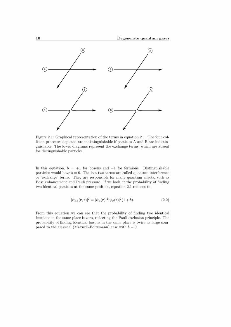
In classical physics, all particles are considered distinguishable, even if they areidentical in the sense that all intrinsic properties are the same. To illustratewhat is meant by this statement, consider two particles involved in a collision.In principle, one could label the particles A and B, and follow their trajectorybefore, during and after the collision. For microscopic particles, the Heisenberguncertainty relation prevents the observer from knowing the exact trajectory ofeach particle. Hence, it is impossible to know after the collision which particlewas A en which was B. Actually, the scattering properties of quantum particlesdepend on the symmetry of the two-particle wave function that describes theparticles. Two-particle wave functions describing bosons are symmetric, andthose describing fermions are antisymmetric with respect to interchanging thetwo particles. The effect of the different symmetry is expressed in the followingformula for the probability density resulting from the two-particle wave functionψαβ(A,B) (see also figure 2.1) [3]:
|ψαβ(A,B)|2 =12[ψ∗
α(A)ψα(A)ψ∗β(B)ψβ(B) + ψ∗
β(A)ψβ(A)ψ∗α(B)ψα(B)
+bψ∗α(A)ψβ(A)ψ∗
β(B)ψα(B) + bψ∗β(A)ψα(A)ψ∗
α(B)ψβ(B)] (2.1)
10 Degenerate quantum gases
A B
B A
A
B
B
A
Figure 2.1: Graphical representation of the terms in equation 2.1. The four col-lision processes depicted are indistinguishable if particles A and B are indistin-guishable. The lower diagrams represent the exchange terms, which are absentfor distinguishable particles.
In this equation, b = +1 for bosons and −1 for fermions. Distinguishableparticles would have b = 0. The last two terms are called quantum interferenceor ‘exchange’ terms. They are responsible for many quantum effects, such asBose enhancement and Pauli pressure. If we look at the probability of findingtwo identical particles at the same position, equation 2.1 reduces to:
|ψαβ(r, r)|2 = |ψα(r)|2|ψβ(r)|2(1 + b). (2.2)
From this equation we can see that the probability of finding two identicalfermions in the same place is zero, reflecting the Pauli exclusion principle. Theprobability of finding identical bosons in the same place is twice as large com-pared to the classical (Maxwell-Boltzmann) case with b = 0.

2.1 Classical and indistinguishable particles 11
Quantum distribution functions
The indistinguishability of quantum particles also influences the distribution ofparticles over the available energy states in thermal equilibrium. Again, thereis a difference between bosons and fermions. As is very nicely explained byFeynman in his celebrated Lectures on Physics [4], the sole assumption of indis-tinguishability in the absence of any exclusion principle leads to the predictionthat the probability for a particle to enter a particular state is increased by afactor (n+ 1), if there are n identical particles present in this state. This Boseenhancement effect can be readily applied to a system with two energy levelsseparated by hω. Statistical mechanics tells us that in thermal equilibrium theratio of the number of particles in the ground state Ng and excited state Ne isgiven by:
Ne
Ng= e−hω/kBT , (2.3)
where kB is Boltzmann’s constant and T is the temperature. Now assume thesystem under discussion is an ensemble of atoms in an electromagnetic field andn is the average number of photons present in a given mode. Then the emissionrate into that mode will be equal to Ne(n + 1) times the emission rate if nophotons are present. From the reversibility of the process follows that the rateof absorption of photons from the field is equal to Ngn times this same unknownemission rate. But the two rates will be equal in thermal equilibrium:
Ngn = Ne(n+ 1). (2.4)
One can see that the emission rate does not appear in the above equation.Combining relation 2.4 with equation 2.3 yields:
n
n+ 1= e−hω/kBT , (2.5)
which can be solved for the mean number of photons in a mode with frequencyω:
n =1
ehω/kBT − 1. (2.6)
This distribution function is called the Bose-Einstein distribution and appliesequally to massive bosons. The derivation of the analogous expression for theother type of indistinguishable particles, fermions, is more cumbersome andless elegant. One has to resort to counting all possible ways of distributingN particles in energy states belonging to M different systems with an infinite
12 Degenerate quantum gases
number of energy levels, with the restriction that only one particle per state isallowed (because of the Pauli principle or, equivalently, the antisymmetry of thefermionic wave functions) [3]. The result is just as simple as for bosons, though.The only difference is that the minus sign in equation 2.6 is replaced by a plussign.
2.2 Bose-Einstein condensation
2.2.1 Introduction
In 1925, Albert Einstein predicted a quantum phase transition for bosons [5]1.Ever since, people have tried to establish this transition (later called Bose-Einstein condensation (BEC)) in systems that could be used to study the phe-nomenon in detail. As early as 1938, it was realised that the then newly dis-covered superfluid properties of liquid 4He at temperatures below 2.18 K [7, 8]were a manifestation of Bose-Einstein condensation. The superfluidity (fric-tionless motion) is due to the fact that the atoms are in the ground state ofthe system and thus cannot lose energy by friction. Liquid helium, however, isa strongly interacting system, which complicates the comparison with theory.Furthermore, only about 10% of the atoms are condensed.
The first ‘pure’ BEC, in a dilute gas, was created in the group of CarlWieman and Eric Cornell (with 87Rb) at JILA in 1995 [9], quickly followed bythe group of Wolfgang Ketterle at MIT [10], who used 23Na, and the Rice groupof Randy Hulet (7Li) [11]. Wieman, Cornell and Ketterle shared the Nobel Prizein 2001 for their achievements. All groups mentioned started from a magneto-optical trap (MOT) and subsequently performed forced evaporative cooling ina magnetic trap. Ketterle’s group was able to show matter wave interference oftwo independent BECs, demonstrating the macroscopic first order coherence ofthe system [12].
2.2.2 Theory
Bose-Einstein condensation is a quantum phenomenon in the sense that it relieson the fact that particles that are confined in a potential well can only assumediscrete energy states. The values of the allowed energies depend on the nature
1Indian physicist Satyendra Nath Bose developed a theory for photon statistics but couldnot get his work published. He sent his manuscript to Einstein, who recognized its importanceand made sure it was published [6]. Einstein subsequently extended the theory to massivebosons with a fixed number of particles.
2.2 Bose-Einstein condensation 13
of the potential. Above the critical temperature TC , at which the Bose-Einsteincondensation takes place, the atoms are distributed over the available energystates in a way that depends on the temperature of the system. If we considernon-interacting identical bosons, the mean occupation number f(εν) of a singleparticle state with energy εν is given by (see section 2.1):
f(εν) =1
e(εν−μ)/kBT − 1. (2.7)
In this equation, μ is the chemical potential. It is the energy required to addone particle to the system and can be calculated from the condition that thetotal number of atoms should equal the sum of occupancies of the individuallevels [13]:
N =∑
ν
1e(εν−μ)/kBT − 1
. (2.8)
It follows from equation 2.8 that the chemical potential rises if the temperatureis lowered. As can be seen from equation 2.7, the chemical potential can neverexceed the value ε0 of the lowest energy state, otherwise the occupation numberof this state would be negative. It also follows from equation 2.7 that the meanoccupation number of any individual excited state is always lower than thatof the ground state. This means that below a certain temperature (or abovea certain number of atoms) the sum of the occupation numbers of the excitedstates will inescapably become significantly smaller than the total number ofatoms N . The remainder of the atoms will be accommodated in the groundstate, and a Bose-Einstein condensate is created.
The transition of a system to the quantum degenerate regime coincides with thepoint at which the wavelength of the particles becomes comparable to the inter-particle spacing. The figure of merit is the phase space density: nλdB, whereλdB = (2πh2/mkBT )1/2 is the thermal de Broglie wavelength of the atoms andn is the density of the cloud. A combination of lowering the temperature andincreasing the density will thus eventually lead to quantum degeneracy. Forbosons, a quantum phase transition occurs at nλdB ≈ 2.612, leading to theformation of a BEC. A similar phase transition does not exist for fermions, butbelow the Fermi temperature the effects of Pauli pressure become apparent insystems of identical fermions (see section 2.3).
The temperature at which the condensation takes place depends on the charac-teristics of the trapping potential and also (weakly) on the interactions between

14 Degenerate quantum gases
the atoms. For a non-interacting gas in a harmonic potential:
U(r) =12m(ω2
xx2 + ω2
yy2 + ω2
zz2) (2.9)
with a geometrical average of the oscillator frequencies ω = (ωxωyωz)1/3, thetransition temperature TC can be calculated to be [2]:
TC =hω
kB
(N
ζ(3)
)1/3
≈ hω
kB
(N
1.202
)1/3
, (2.10)
where ζ(s) =∑∞
n=1 n−s is the Riemann zeta function. The number of atoms in
the ground state, N0, is a function of the degeneracy parameter T/TC :
N0
N= 1 −
(T
TC
)3
for T < TC , (2.11)
resulting in a pure BEC only for T = 0 (see figure 2.2).
Interactions
The strength of the interactions between the atoms can be described by a singleparameter a. This parameter is called the s-wave scattering length and givesthe two-body collision cross section σ(k) at low temperatures [14, 15]:
σ(k) =8πa2
1 + k2a2(2.12)
where hk is the momentum of the atom. The same parameter a also governsthe mean field potential experienced by the atoms in the condensate. TheSchrodinger equation for a system of harmonically trapped atoms experiencinga mean field potential, is known as the Gross-Pitaevskii equation [16]:
ihdψ
dt= − h2
2m∇2ψ + U(r)ψ + U |ψ|2ψ. (2.13)
The parameter U = 4πh2a/m, proportional to the scattering length, describesthe mean field effect due to the interactions between the atoms. If the scatter-ing length is negative (attractive interaction), the condensate becomes unstableand will collapse if the number of particles in the condensate surpasses a certaincritical value. If the scattering length is positive (as in the case of 4He∗), the

2.2 Bose-Einstein condensation 15
0.0 0.2 0.4 0.6 0.8 1.0 1.2 1.4T/TC
0.0
0.2
0.4
0.6
0.8
1.0
N0/N
Figure 2.2: Condensate fraction N0/N as a function of the scaled temperatureT/TC . A pure BEC exists only at T = 0, the condensate fraction is negligiblefor T > TC .
condensate will be stable. In the limit of strong interactions (nU � hω), thekinetic energy term of equation 2.13 can be neglected compared to the interac-tion term. In this so-called Thomas-Fermi approximation the density profile ofthe condensate is given by the simple equation [16]:
nc(r) = max(μ− U(r)
U, 0)
(2.14)
where the chemical potential is given by:
μ =12hω
(15
N0a
(h/mω)1/2
)2/5
(2.15)
In the Thomas-Fermi approximation the density profile of an harmonicallytrapped condensate takes the form of an inverted parabola with radius:
Rα =
√2μmω2
α
(2.16)

16 Degenerate quantum gases
Expansion
Finally, when the trap is switched off, the condensate will expand ballistically,converting the mean field energy into kinetic energy. In the Thomas-Fermiapproximation, the condensate density profile remains an inverted parabola ofwhich the radii can be calculated as a function of expansion time [17]:
Rρ(t) = Rρ(0)√
1 + τ2 (2.17)
Rz(t) = Rz(0)(1 +(ωz
ωρ
)2 [τarctanτ − ln
√1 + τ2
]), (2.18)
where τ = ωρt.The binding energy of the least-bound state of the interaction potential of
spin-polarised 4He∗ has been measured to great accuracy using two-photon pho-toassociation spectroscopy [18]. From this binding energy, a scattering lengthof a = 7.5105(25) nm can be deduced [19]. From the above equations it is clearthat if the harmonic trap frequencies are known, the number of atoms in thecondensate can in principle be deduced from the expansion of the condensate.One has to assume, though, that the trap is switched off fast with respect tothe timescale set by the inverse of the trap frequencies. This criterion was notsatisfied in our experiment. The condensate also saturated our MCP detector,therefore it was hard to determine the exact number of atoms in our condensate.Chapter 5 describes the production of a condensate of metastable 4He atoms insome detail.
2.3 Quantum degenerate Fermi gas
2.3.1 Introduction
For a long time, the main focus within the laser cooling community has beenon the realisation of Bose-Einstein condensation, and therefore on bosons. Nowthat this long-standing goal has been reached, at least part of the focus of thefield seems to shift toward the production of ultracold fermions. Fermions donot undergo a quantum phase transition below a critical temperature, thoughcondensation of bosonic pairs of fermions has been demonstrated [20, 21]. For-mation of Cooper pairs in ultracold clouds of fermions may provide insight intothe mechanisms of high-temperature superconductivity [22]. Fermions in anoptical lattice, to give another important example, are an ideal experimentalmodel system of electrons in solid state matter. The system mimics solid state
2.3 Quantum degenerate Fermi gas 17
systems and many parameters, such as the potential depth of the optical lattice,or the interaction strength between the atoms, can be varied at will.
2.3.2 Theory
The interesting Fermi systems mentioned above are created starting from anultracold cloud of atoms, usually close to the Fermi temperature. Ultracoldsamples are produced using forced evaporative cooling, which relies on thermal-isation of the sample by elastic collisions. Due to the antisymmetric nature ofthe fermionic wave function, collisions between identical fermions are highly sup-pressed at low temperatures. The main contribution to the collision cross sectionis the lowest partial wave, corresponding to zero relative angular momentum ofthe two colliding atoms. This s-wave scattering does not occur between identi-cal fermions, because of the symmetry of the process and the anti-symmetry ofthe wave functions. Therefore, one needs a second component with which thefermions can be cooled. In principle, this second component can be a differentspin state of the same atomic species, a different isotope of the same species,or a different element. Ignoring the possibility of sympathetic cooling of 3He∗
with ground state atoms of a different element, only cooling with 4He∗ appearsto be possible. This is because in the case of 3He∗, the occurrence of Penningionisation (see section 4.5.1) requires all atoms to be in the fully stretched spinstate (F,mF ) = (3/2, 3/2). Adding for example (F,mF ) = (3/2, 1/2) to thesample, would result in destructive ionising collisions until finally only atoms inthe fully stretched spin state are left.
If the efficiency of the sympathetic cooling is concerned, a mixture of a bosonand a fermion would be better than a fermion-fermion mixture [23]. When thedegenerate regime is approached, more and more low-lying energy levels will beoccupied. These occupied states are not available for fermions as final statesafter a scattering process, which will limit the scattering rates. For fermion-fermion mixtures this Pauli blocking effect is twice as large as for boson-fermionmixtures. In our experiment, however, we have seen a disadvantage of the useof bosons. As soon as a BEC is created, the Fermi-cloud and the BEC willhave a reduced spatial overlap (due to the small size of the condensate), as wellas increased three-body losses. Actually, at certain experimental parameters,a complete spatial separation of the bosons and fermions is predicted [24, 25].This phenomenon is called phase separation.
At zero temperature, all quantum levels of the harmonic potential of themagnetic trap are filled from the bottom up. The energy of the most energetic

18 Degenerate quantum gases
occupied state is called the Fermi energy EF . The Fermi temperature [13] thatis associated with the Fermi energy is given by: TF = EF /kB:
TF =hω
kB(6N)1/3 (2.19)
The degree of degeneracy is usually expressed in terms of the degeneracyparameter T/TF . The lowest obtainable value of this degeneracy parameterdepends on the ratio of the heat capacities of the actively cooled bosons andsympathetically cooled fermions. In the classical regime, the heat capacity isCC = 3NkB. One expects the cooling to break down if the heat capacities ofthe cooling and cooled species become equal. For classical particles, this wouldhappen if the number of atoms of both species become equal. In the quantumregime, the situation becomes slightly more complicated. We have, for T < TC
and T < TF , respectively [23]:
CB = 12ζ(4)ζ(3)
NBkB
(T
TC
)3
, (2.20)
CF = π2NFkBT/TF . (2.21)
Depending on the exact conditions during the evaporative cooling process, acombination of the classical and quantum expressions should be used to calculatethe conditions that can be obtained at the end of the process.
Chapter 6 describes the production of a quantum degenerate Fermi gas of3He∗, that was obtained by sympathetic cooling with 4He∗.
Chapter 3
Quantum correlations
When a cloud of cold atoms gets close to the quantum degenerate regime,the wave character of the particles becomes important for a description of itsbehaviour. Several concepts and phenomena that are well-known from the the-ory of electromagnetic waves can be applied to ultracold atoms. Especiallyimportant is the concept of coherence. An experiment in which the coherenceof a cloud of ultracold helium atoms was investigated, was conducted in ourlab in collaboration with the cold helium group of the Institute d’Optique inOrsay1, France. The resulting article is included in this thesis as chapter 7.This experiment, which is the atomic analog of a seminal experiment performedby Robert Hanbury Brown and Richard Twiss in 1956 [26], studied the second-order coherence (pair correlations) of the ensemble of atoms. The main aim ofthis chapter is to give some theoretical and historical background to chapter 7.
3.1 Quantum coherence functions
The development of quantum optics and quantum coherence theory was greatlystimulated by the demonstration and implementation of intensity interferometryby Robert Hanbury Brown and Richard Twiss (HBT) [26, 27, 28]. A descrip-tion of the coherence length of a beam of light and the associated correlationsbetween intensity fluctuations at different times and locations in the beam couldbe constructed within a classical framework. The fact that the photons weredetected by means of the photo-electric effect, however, meant that a quantum
1After our collaboration, the group moved to Palaiseau.
20 Quantum correlations
mechanical description was required to understand all details of the process.Purcell [29], Fano [30] and Glauber [31, 32], among others, provided a fullyquantum mechanical explanation of the HBT-effect. Quantum optics is a goodstarting point for a treatment of the atomic analog of intensity interferometry:the measurement of correlations between atom pairs.
3.1.1 The Hanbury Brown-Twiss effect
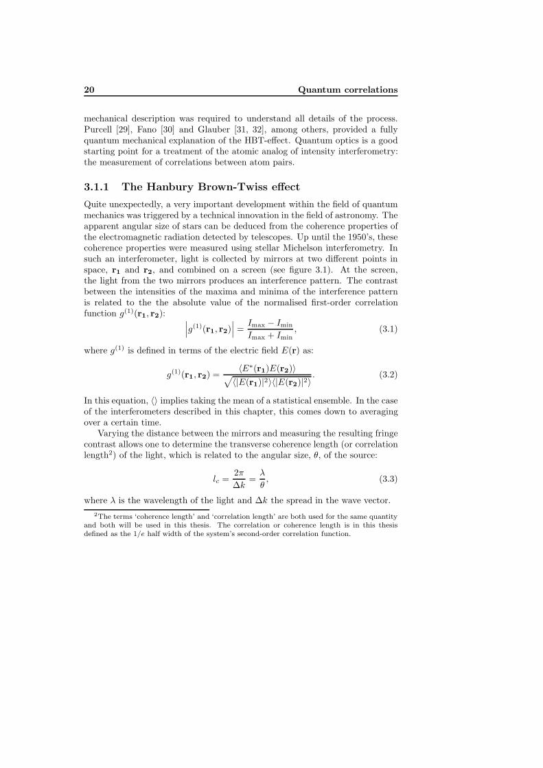
Quite unexpectedly, a very important development within the field of quantummechanics was triggered by a technical innovation in the field of astronomy. Theapparent angular size of stars can be deduced from the coherence properties ofthe electromagnetic radiation detected by telescopes. Up until the 1950’s, thesecoherence properties were measured using stellar Michelson interferometry. Insuch an interferometer, light is collected by mirrors at two different points inspace, r1 and r2, and combined on a screen (see figure 3.1). At the screen,the light from the two mirrors produces an interference pattern. The contrastbetween the intensities of the maxima and minima of the interference patternis related to the the absolute value of the normalised first-order correlationfunction g(1)(r1, r2): ∣∣∣g(1)(r1, r2)
∣∣∣ = Imax − Imin
Imax + Imin, (3.1)
where g(1) is defined in terms of the electric field E(r) as:
g(1)(r1, r2) =〈E∗(r1)E(r2)〉√〈|E(r1)|2〉〈|E(r2)|2〉 . (3.2)
In this equation, 〈〉 implies taking the mean of a statistical ensemble. In the caseof the interferometers described in this chapter, this comes down to averagingover a certain time.
Varying the distance between the mirrors and measuring the resulting fringecontrast allows one to determine the transverse coherence length (or correlationlength2) of the light, which is related to the angular size, θ, of the source:
lc =2πΔk
=λ
θ, (3.3)
where λ is the wavelength of the light and Δk the spread in the wave vector.2The terms ‘coherence length’ and ‘correlation length’ are both used for the same quantity
and both will be used in this thesis. The correlation or coherence length is in this thesisdefined as the 1/e half width of the system’s second-order correlation function.

3.1 Quantum coherence functions 21
M1
M3
M4
M2
S1
S2
P
r1
r2
k k’
r1 r2
φ
Figure 3.1: Schematic of a Michelson stellar interferometer. Light from a distantobject is collected on movable mirrors M1 and M2, located at positions r1 andr2. The light is sent through diaphragms S1 and S2 that act as point sourcesand create an interference pattern at point P on a screen. The intensity of thelight measured at P gives the first-order correlation function g(1) as a functionof the distance between M1 and M2: Δr = r2 − r1. The resulting correlationlength gives the angular size of the light source, using equation 3.3. The insetshows two incident plane waves with wave vectors k and k′, as introduced inequation 3.5. The angle φ is equal to the angular size of the source θ in case theplane waves are emitted from the right and left edges of the star, respectively,and provided that Δr is much smaller than the transverse size of the source.

22 Quantum correlations
Longitudinal coherence is the coherence along the direction of propagationof the light and is usually expressed as a coherence time tc:
tc =2πΔω
=h
ΔE, (3.4)
where Δω is the spectral width of the light. The expressions for the trans-verse and longitudinal coherence are both limiting cases of the same generalrequirement, originating from the fact that coherence is observed only withinan elementary cell in phase space. The value of 2π/Δk ultimately governs thecoherence properties of the system. For the transverse coherence length, thelight is taken to be monochromatic, such that Δk is fully determined by thespatial spread in the wave vector. The coherence time, on the other hand, isdependent only on the frequency spread if one considers light with Δθ = 0.
In addition to the fact that Michelson- and other types of amplitude inter-ferometry are very sensitive to the alignment of the interferometer, they alsosuffer from an inherent sensitivity to variations in the refractive index of theatmosphere. This can be demonstrated if we consider the light to be madeup of two monochromatic plane waves with wave vectors k and k′ [33]. Theintensity of the light on the screen becomes:
I ∝ 〈|Ek(r1) + Ek′(r1) + Ek(r2) + Ek′(r2)|2〉⇒ I/I0 = 4 + 4cos((k + k′) · Δr/2)cos(kΔrφ/2), (3.5)
where Δr = r2 − r1 is the vector connecting the two mirrors and φ is the anglebetween the incident rays (see figure 3.1). The first cosine is sensitive to themodulus of k + k′ and tends to vary rapidly, obscuring the value of the secondcosine term, which contains the relevant information.
Hanbury Brown and Twiss knew that there was a very simple relationbetween the first- and second-order correlation function of light emitted from achaotic source, like a star [34]:
g(2) = 1 + |g(1)|2. (3.6)
Measuring the second-order correlation function would thus also provide thedesired information on the coherence length. Expressed in terms of intensities,g(2) can be written down as:
g(2)(x1, x2) =〈I(x1)I(x2)〉〈I(x1)〉〈I(x2)〉 , (3.7)

3.1 Quantum coherence functions 23
0.0 0.5 1.0 1.5 2.0 2.5 3.00.0
0.5
1.0
1.5
2.0
g(2
)(Δ
z)
pair separation Δz (a.u.)
lc
η
Figure 3.2: Normalised second-order correlation function g(2)(Δz), with Δx =Δy = Δt = 0, of a thermal ensemble of particles. The dashed line shows g(2) forbosons, and the dotted line is expected for fermions. The solid line is an exampleof the expected experimental result for bosons, if the detector resolution is notnegligible compared to the correlation length. In that case, the amplitude of thebunching signal is reduced and the contrast parameter η has to be introduced(see also section 3.4).
where the vector x = (r, t) is introduced to make the definition more general.The deviation of g(2) from unity for interparticle distances smaller than the
coherence length indicates ‘bunching’ of photons: the probability of finding twophotons close to each other is larger than expected for statistically independentparticles. This can be seen as a result of the fact that the particles are indistin-guishable bosons and have to obey Bose-Einstein statistics. Fermions, on theother hand, display the opposite effect: ‘antibunching’.
Multiplication and integration of the electronic signals generated by two pho-todetectors yields a signal directly proportional to the second-order correlationfunction:
C = 〈I(x1)I(x2)〉 = I20 g
(2)(x1, x2), (3.8)
where I0 is the intensity of the light on a single detector. If we consider the

24 Quantum correlations
M1
LPX
M2
LP
r1
r2
detector
θ
lightsource
Figure 3.3: Schematic of a stellar intensity interferometer, invented by HanburyBrown and Twiss. Light from a distant object is collected on mirrors M1 andM2, located at positions r1 and r2, and sent onto photodetectors. The result-ing signals are sent through low pass filters (LP ) before they are multipliedin the correlator X . The resulting signal is proportional to the second-ordercorrelation function g(2) and is a function of the distance between M1 and M2.The correlation length gives the angular size θ (see inset) of the light source viaequation 3.3.
3.1 Quantum coherence functions 25
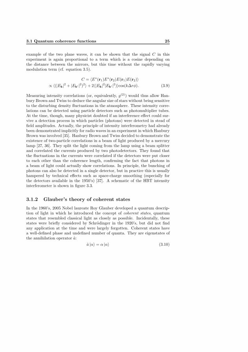
example of the two plane waves, it can be shown that the signal C in thisexperiment is again proportional to a term which is a cosine depending onthe distance between the mirrors, but this time without the rapidly varyingmodulation term (cf. equation 3.5).
C = 〈E∗(r1)E∗(r2)E(r1)E(r2)〉∝ 〈(|Ek|2 + |Ek′ |2)2〉 + 2〈|Ek|2|Ek′ |2)〉cos(kΔrφ). (3.9)
Measuring intensity correlations (or, equivalently, g(2)) would thus allow Han-bury Brown and Twiss to deduce the angular size of stars without being sensitiveto the disturbing density fluctuations in the atmosphere. These intensity corre-lations can be detected using particle detectors such as photomultiplier tubes.At the time, though, many physicist doubted if an interference effect could sur-vive a detection process in which particles (photons) were detected in stead offield amplitudes. Actually, the principle of intensity interferometry had alreadybeen demonstrated implicitly for radio waves in an experiment in which HanburyBrown was involved [35]. Hanbury Brown and Twiss decided to demonstrate theexistence of two-particle correlations in a beam of light produced by a mercurylamp [27, 36]. They split the light coming from the lamp using a beam splitterand correlated the currents produced by two photodetectors. They found thatthe fluctuations in the currents were correlated if the detectors were put closerto each other than the coherence length, confirming the fact that photons ina beam of light could actually show correlations. In principle, the bunching ofphotons can also be detected in a single detector, but in practice this is usuallyhampered by technical effects such as space-charge smoothing (especially forthe detectors available in the 1950’s) [37]. A schematic of the HBT intensityinterferometer is shown in figure 3.3.
3.1.2 Glauber’s theory of coherent states
In the 1960’s, 2005 Nobel laureate Roy Glauber developed a quantum descrip-tion of light in which he introduced the concept of coherent states, quantumstates that resembled classical light as closely as possible. Incidentally, thesestates were briefly considered by Schrodinger in the 1920’s, but did not findany application at the time and were largely forgotten. Coherent states havea well-defined phase and undefined number of quanta. They are eigenstates ofthe annihilation operator a:
a |α〉 = α |α〉 (3.10)

26 Quantum correlations
Coherent states can be constructed from so-called number states |n〉, that areeigenstates of the number operator:
n |n〉 = n |n〉 (3.11)
|α〉 = e−12 |α|2
∞∑n=0
αn
√n!
|n〉 . (3.12)
Equation 3.10 implies that detection of a particle does not change a coherentstate: hence the detection processes are independent. This is why the second-order correlation function for Bose condensed systems and laser sources (bothfully coherent states) have a constant value (unity). Detection of a particlein such a fully coherent system has no effect on the state of the system, andhence the detection probability of a second particle will be independent from thedetection of the first particle. This yields a flat correlation function. For thermalsources, this is not true: detection of one particle removes one quantum from thestate and thus changes the state. This will influence the probability of detectinga second particle within the coherence volume of the first one. As described inchapter 7, a thermal source shows either ‘bunching’ or ‘antibunching’ of particlesas a result of the exchange term of the two-particle wave function for bosonsand fermions, respectively.
Types of quantum coherence
Coherent states can be seen as translations of the vacuum state (i.e., the har-monic oscillator ground state, which is a coherent state with α = 0). They havea minimum product of the conjugate variables phase and amplitude/number aswell as a minimum position and momentum uncertainty. Number states havea fully defined number of quanta and undefined phase. The opposite, a statewith fully defined phase, does not exist, since no hermitian phase operator canbe formulated [38]. One could therefore say that truly ‘classical’ light does notexist.
Any single-mode field is first-order quantum coherent, be it a number stateor coherent state. In amplitude interference experiments, no distinction can bemade between number and coherent states, even though the photon distributionsare strikingly different. One needs second-order or intensity interferometry todistinguish between the two cases. Atoms are always in a number state, becausethey are massive particles.
3.2 Extension to massive particles 27
In case of first-order coherence, g(1) = 1. A quantum field is said to besecond-order coherent if |g(1)(x1, x2)| = 1 and g(2)(x1, x2;x2, x1) = 1 [38]3.According to this definition, a coherent state |α〉 is second-order coherent, evenif it is multimode. The photons in such a state will arrive on a detector accordingto a Poisson distribution. Considering a single-mode thermal state, g(2)(τ) = 2,where τ = t2 − t1, indicating a higher probability of detecting two photons at afixed position, independent of the time delay. This is not what Hanbury Brownand Twiss observed, though. Even though the analysed light was made quasi-monochromatic using a filter, the light could still be described as a multimodethermal state, for which the following general relation holds (cf. equation 3.6):
g(2)(τ) = 1 + |g(1)(τ)|2. (3.13)
For light with a Lorentzian spectrum this yields a correlation function with a‘bunching peak’:
g(2)(τ) = 1 + e−2|τ |/τ0. (3.14)
So one can speak of bunching if g(2)(0) > g(2)(τ) for τ > 0. Theoretically, photonantibunching would occur for g(2)(0) < g(2)(τ), but even though a single modenumber state |n〉 would give g(2)(0) < 1 and thus exhibit classically forbiddensub-Poissonian statistics, the condition g(2)(0) < g(2)(τ) is not fulfilled, sinceg(2)(τ) is constant. Therefore, this photon state does not show antibunching.Light created in resonance fluorescence, on the other hand, where a single two-level atom is driven by a resonant laser field, does exhibit photon antibunching.Such a light field can be considered highly non-classical [38, 39].
3.2 Extension to massive particles
Both the experiments and theoretical framework described in the previous sec-tion deal with photons, i.e., massless bosons. Quantum mechanics tells us thatthe description of light quanta is not so different from that of massive particles.Actually, the theory described in the previous section can just as well be appliedto matter wave fields, provided that one introduces some restrictions like par-ticle number conservation. One finds that the correlation function g(2) governstwo-body loss processes in samples of atoms, because g(2)(0) is the chance thattwo particles are at the same position (e.g. collide). The mean-field energy(see section 2.2.2) is due to elastic collisions and is proportional to the integral
3In this second quantisation picture, the order of the operators has to be specified, sincethey do not commute.

28 Quantum correlations
over the density squared times g(2)(r). The mean field is therefore higher fora thermal cloud of the same density since, as shown above, g(2)(0) = 2 for athermal sample and g(2)(0) = 1 for a coherent state. In general, g(n)(0) = 1 fora condensate and g(n)(0) = n! for a thermal distribution.
Coherence theory seems to predict that the HBT-effect can also be observedin systems of massive particles, such as atoms. Furthermore, fermionic atoms areexpected to display exactly the opposite behaviour. The predicted antibunchingof fermions would be more interesting than the bunching in the sense that itis a pure quantum phenomenon: classical wave theory can be used to modelbunching of light, but antibunching has no classical analogue.
Actually, as early as 1960, measurements on pp collisions performed with theBevatron accelerator showed that angular correlations were dependent on quan-tum interference effects, just like the astronomical HBT effect [40]. Accordingto Abraham Pais, who was involved in the Bevatron experiment, the conceptof intensity interference as applied in particle physics was conceived indepen-dently: it was simply invoked as an explanation of the experimental data. It hasbecome a standard technique in the analysis of high energy collisions [41, 42],since it can be used to determine the size of sources of secondary particles. Itcan of course only be used for identical reaction products, and one has to becareful about the Coulomb interaction for particles such as π+, π−, K+, orK−. In general, a huge advantage of intensity interferometry is that one canget information from the second-order correlations that is not contained in theoverall density profile. It is believed that HBT-type of measurements can beused to probe the nature of various kinds of exotic quantum systems [43].
It was realised from the start that massive fermions should display anti-bunching behaviour, and anti-correlations in relative momenta of fermions havebeen used in subatomic physics experiments since the late seventies [42]. It tookuntil 1999, however, before the first experiments demonstrating antibunching ofelectrons in semiconductor devices were reported [44, 45], followed in 2002 by theobservation of electron antibunching in a free electron beam [46]. Antibunchingof free neutrons was finally reported in 2006 [47].
In this type of experiments, the detection of quantum statistical effects hasalways been hampered by the low phase space density of the radiation fields.The development of techniques based on laser- and evaporative cooling hasprovided a new source of massive particles with a high phase space density:ultracold atoms. A major advantage of the use of neutral atoms for intensityinterference experiments is of course that one does not have to account forthe strong Coulomb interactions that play a role in experiments with chargedparticles. On the other hand, neutral atoms are in general harder to detect than
3.3 Correlation experiments with cold atoms 29
charged particles. In the next section, a few intensity interference experimentswith cold atoms will be described. The last section of this chapter is devotedto a theoretical description of the experiment that we have performed ourselvesand of which the results can be found in chapter 7.
3.3 Correlation experiments with cold atoms
Several intensity interference experiments with cold atoms has been conductedto date. In this section, the studies that are interesting in relation with thisthesis are briefly reviewed.
Metastable neon MOT (Tokyo)
The first correlation experiment using cold atoms was an experiment by Yasudaand Shimizu in 1996 [48]. They used a magneto-optical trap (MOT) containingmetastable neon. Atoms were coupled out from the MOT using a laser thatpumped atoms into an untrapped state. The atoms that fell downward under theinfluence of gravity were focused onto the detection unit by electrostatic lenses.The atoms released an electron from the surface of a gold coated mirror andthis electron was subsequently attracted toward a microchannel plate detector.In this experiment, the temporal correlations in the arrival time of the atomsin the continuous atomic beam were measured. Bunching of the neon atomsarriving on the detector on a time scale of 0.5 μs was observed. The spatialcoherence of this system was too small to be measured, though.
Rubidium BEC (Zurich)
Another experiment in which the temporal correlations were measured, wasperformed by Ottl et al. in the group of Esslinger in Zurich [49]. This time, aBose-Einstein condensate of rubidium was used. The atoms were coupled out bya radio-frequency field and detected when they fell through a high finesse opticalcavity. The atoms disturb the light field inside the cavity and this disturbanceis detected. In this way they were able to detect single atoms, even thoughthe fact that they used ultracold ground state atoms excluded the possibility ofusing microchannel plate-like particle detectors. When the atoms were coupledout in a coherent way, the expected flat pair correlation function was obtained.A quasi-thermal distribution was created by adding white noise of a particularbandwidth to the outcoupling rf frequency. The temporal coherence was shownto be directly related to the frequency width of the white noise.
30 Quantum correlations
Atoms released from an optical lattice (Mainz)
A different approach in detecting intensity correlations in ensembles of groundstate atoms was taken by the group of Bloch in Mainz [50]. They analysedthe noise correlations in absorption images taken of atoms released from anoptical lattice. It was shown that the quantum mechanical shot noise showedspatially periodic correlations that could be assigned to the occupation of linearmomentum states that make up the Bloch states in the lattice. No periodicity isobserved in the density profile of the released cloud (no first-order interference),but the effect of Bose enhancement shows up in the spatial correlations. Thesame technique was applied in a similar experiment in Mainz, in which fermionicpotassium was trapped [51]. The same periodic structure was observed, but inthis case showing anticorrelations.
Metastable helium (Orsay)
In 2005, the cold helium group of the Institute d’Optique in Orsay used aposition-sensitive microchannel plate detector to detect clouds of bosonic meta-stable helium atoms that were released from a magnetic trap [52]. In this pulsedexperiment, a 3D snapshot of the ballistically expanding cloud was made, andthe pair-correlation function along the three Cartesian axes was constructed.The correlations observed in clouds above and below the condensation thresholdwere compared. The BEC showed a flat pair correlation function, whereasthe thermal cloud exhibited bunching over a distance depending on the sourcesize in the respective directions. In a more recent experiment conducted bythis group, correlated atom pairs, produced by two colliding Bose condensates,have been observed [53]. The position-sensitive detector was also used in ourcollaboration with the Orsay group in which the HBT-effect was measured for3He∗ and 4He∗ (see chapter 7). In the following section some background theoryfor the experiment described in chapter 7, based on the article of Viana Gomeset al. [54], is discussed.
3.4 HBT experiment with a ballistically expanding cloud 31
3.4 HBT experiment with a ballistically expand-
ing cloud
The atoms are described as a matter wave field in second quantisation, wherewe can define the field operators:
Ψ†(r) =∑
j
ψ∗j (r)a†j , Ψ(r) =
∑j
ψj(r)aj . (3.15)
The wave functions ψj are energy eigenfunctions associated with energy levelj. The operators a†j and aj create and annihilate one particle in state |ψj〉respectively. The operators Ψ†(r) and Ψ(r) create and annihilate a particle atposition r.
The first- and second-order atomic correlation functions are now defined as:
G(1)(r, r′) = 〈Ψ†(r)Ψ(r′)〉 (3.16)
G(2)(r, r′) = 〈Ψ†(r)Ψ(r)Ψ†(r′)Ψ(r′)〉. (3.17)
In the remainder of this section, it will be shown how the second-ordercorrelation function G(2) can be expressed in terms of first-order correlationfunctions G(1), as already shown earlier in this chapter for the normalised photoncorrelation functions. More specifically, the expressions for both bosons andfermions will be derived, in order to show the origin of the different behaviourof the two types of particles. To accomplish this feat, a number of algebraicrelations will be introduced, that will subsequently be used for the reduction ofG(2).
First, the bosonic creation and annihilation operators obey the followingcommutation relations: [
aj , a†k
]= aj a
†k − a†kaj = δjk (3.18)
[a†j , a
†k
]= [aj , ak] = 0. (3.19)
Similar relations exist for the fermionic operators, but now for anticommutators:{aj , a
†k
}= aj a
†k + a†kaj = δjk (3.20)
{a†j , a
†k
}= {aj , ak} = 0. (3.21)

32 Quantum correlations
The correlation functions 3.16 and 3.17 contain ensemble averages 〈. . .〉. Itcan be shown [55] that the ensemble average of any operator O can be expressedas:
〈O〉 = Tr[ρO], (3.22)
whereρ = exp
(β(Ω − H − μN)
)(3.23)
is a density matrix that can be normalised such that 〈ρ = 1〉. In this expressionβ = 1/kBT , H is the Hamiltonian operator, N the number operator and μ isthe chemical potential. Ω is called the thermodynamic or Landau potential.For this derivation, one does not need to know the details of the density matrixoperator. Only the following algebraic relations are needed [55]:
aj ρ = ρajexp (−β(εj − μ)) , (3.24)
anda†j ρ = ρa†jexp (β(εj − μ)) . (3.25)
where εj is the energy associated with the state ψj .If the fact is added that cyclic permutations of operators of which a trace
is taken do not change the value of the trace, one has the tools to derive thelast intermediate result needed to rewrite G(2) in terms of G(1). The derivationis given in appendix A, and the result is just an expression of the thermaldistribution functions:
〈a†j ak〉 =δjk
exp (β(εj − μ)) ∓ 1. (3.26)
From now on, upper (lower) signs are used to apply to bosons (fermions). Inthis way the derivations for bosons and fermions can easily be combined. Onerecognises the Bose-Einstein distribution for bosons (minus sign) and the Fermi-Dirac distribution (plus sign) for fermions in this expression.
Equation 3.26 can be used to find a more explicit expression for G(1):
G(1)(r, r′) = 〈Ψ†(r)Ψ(r′)〉 (3.27)
=∑j,k
〈a†j ak〉ψ∗j (r)ψk(r′) (3.28)
=∑
j
ψ∗j (r)ψj(r′)
exp (β(εj − μ)) ∓ 1. (3.29)

3.4 HBT experiment with a ballistically expanding cloud 33
The analogous explicit expression for the second-order correlation functionis:
G(2)(r, r′) = 〈Ψ†(r)Ψ(r)Ψ†(r′)Ψ(r′)〉. (3.30)
=∑
j,k,l,n
〈a†j aka†l an〉ψ∗
j (r)ψk(r)ψ∗l (r′)ψn(r′) (3.31)
The product of creation and annihilation operators can be written as a sumof three terms. Again the derivation is given in appendix A:
〈a†j aka†l an〉 =
δjk〈a†l an〉 ± δjn〈a†l ak〉 + δjnδlkexp (β(εj − μ)) ∓ 1
. (3.32)
Each of the terms in this equation can now be relatively easily expressed interms of first-order correlation functions G(1) (see appendix). The result is:
G(2)(r, r′) = G(1)(r, r)G(1)(r′, r′) ± |G(1)(r, r′)|2 +G(1)(r, r)δ(r − r′) (3.33)
The last term is called the shot-noise term and is proportional to the number ofparticles N , whereas the first two terms are proportional to N2. For sufficientlylarge systems, the last term can therefore be neglected. When the remainingterms are properly normalised, equation 3.6 is recovered for bosons. Clearly, theexpression for fermionic massive particles is very similar to the one for bosons:the only difference is the minus sign in front of the second term, reflecting thedestructive quantum interference that leads to antibunching.
It can be shown [56] that the wave function of the expanded cloud can beexpressed in terms of the well-known eigenfunctions of a 3D harmonic oscilla-tor potential ψ0
j (r). The wave function after expansion is identical to that inthe trap except for a phase factor that cancels out in second-order correlationmeasurements, and a scaling factor in the coordinates (as given in equation3.36). The expected pair-correlation function G(2) can now be calculated fromequation 3.33.
In our experiments, the time it takes for the cloud to travel toward thedetector (ca. 360 ms), is much larger than the time it takes for the cloud to fall‘through’ the detector plane (ca. 3 ms). Therefore, the detection process canbe treated as if all atoms are detected instantaneously: one obtains a 3D ‘snapshot’ of the cloud. In this snap shot approximation, the second-order correla-tion function as measured in a ballistically expanding cloud of non-interactingthermal massive bosons is given by:
G(2)(r, t; r′, t) =1∏
α(1 + ω2αt
2)
[ρ(r)ρ(r′) + |G(1)(r, r′)|2 − ρ0(r)ρ0(r′)
](3.34)

34 Quantum correlations
where ρ0 is the ground state density that becomes significant only close to orbelow the transition temperature TC if one deals with bosons4. The shot noiseterm present in equation 3.33 has been neglected. For fermions, the last term inequation 3.34 is negligible since no macroscopic occupation of the ground stateis allowed. The expression for G(2) becomes:
G(2)(r, t; r′, t) =1∏
α(1 + ω2αt
2)
[ρ(r)ρ(r′) − |G(1)(r, r′)|2
](3.35)
The coordinates r = (x, y, z) are the scaled variables that can be found fromthe evolution of the initial wave functions in the trap [54]:
x =x√
1 + ω2xt
2y =
y√1 + ω2
yt2
z =H − 1
2gt2√
1 + ω2zt
2. (3.36)
Here H is the distance from the trap to the detector.An interesting consequence of the fact that the expanding wave functions
follow simple scaling rules, is that the correlation lengths lα(t) in direction αare also simply proportional to the correlation lengths in the trap lα(0):
lα(t) = lα(0)√
1 + (ωαt)2. (3.37)
The correlation length in the trap is, for temperatures sufficiently above quan-tum degeneracy, related to the thermal de Broglie wavelength as defined insection 2.2.2: lα(0) = λdB/
√2π.
Bose condensed clouds
As already mentioned in section 3.1.2, atoms in a fully coherent state will notshow any bunching effect. This effect can be easily explained if one realisesthat bunching and antibunching are quantum interference effects that are dueto the exchange terms mentioned in section 2.1. These terms only arise ifone writes down the probability amplitude of a process that consists of two(or more) indistinguishable processes. As also described in chapter 7, for theHBT experiments these processes constitute the detection of particles emittedfrom two source points. In case of a BEC, any two points in the condensate
4The contribution from the ground state is calculated in the canonical ensemble, in contrastwith the terms associated with the thermal atoms. This solves the problem that is created bythe fact that the grand canonical ensemble assumes the existence of a particle reservoir thatdoes not exist for the condensate [54].

3.4 HBT experiment with a ballistically expanding cloud 35
are identical. This means that there is really only one process, and hence noquantum interference. The correlation length of the BEC is equal to the size ofthe condensate. Therefore, the normalised second-order correlation function ofa BEC is a constant, and its value is unity because of the normalisation.
Effects of finite detector resolution
In principle, the correlation functions and corresponding correlation lengths thatare calculated above can be measured. In practice, one is faced with the factthat the spatial resolution of the position-sensitive microchannel plate detector(described in chapter 7) is not negligible compared to the correlation lengthsof the cloud of atoms when it arrives on the detector. The correlation lengththat is measured is actually a convolution of the real correlation length and thedetector resolution function (see section 4.5.2). If the rms width of the detectorresolution function in direction α is dα, then the observed correlation lengthbecomes:
lα →√l2α + (2dα)2. (3.38)
Furthermore, a finite detector resolution results in a reduction of the heightof the bunching and antibunching signals. This is due to the fact that thedetector effectively averages over more than one cell in phase space. The contrastparameter η is a measure of this effect. It can be defined as |g(2)(0) − 1| andbecomes:
η =∏α
√1 + (dα/sα)2
1 + 4(dα/lα)2(3.39)
where sα ≈√
kBTm t is the size of the cloud at the detector.

36 Quantum correlations

Chapter 4
Experimental setup
This chapter describes the main components of the experimental setup, as well asthe sequence in which they are used to prepare ultracold samples of metastablehelium.
4.1 The atomic structure of 3He and 4He
The electronic state of helium that is used in laser cooling experiments is givenin spectroscopic notation as n 2S+1LJ=2 3S1 [3]. This state is formed by twoelectrons in s-orbitals (l = 0) and with parallel spins, such that S = s1 + s2 = 1and L = l1 + l2 = 0. The total electronic angular momentum quantum numbercan take only one value: J = |J| = |L + S| = 1. The principal quantum numberassociated with one electron (in the lowest hydrogenic state) is n = 1. In atriplet spin state, the other electron must be in an excited state due to thePauli principle. The n in n 2S+1LJ denotes the principal quantum number ofthe excited electron. The 2 3S1 state is called a metastable state because ofits long lifetime, which is due to the fact that it cannot decay to the 1 1S0
ground state via an electric dipole transition. Only one of the electrons can bein an excited state, since the energy needed to excite both electrons exceedsthe 24.6 eV ionisation threshold [3]. Metastable 2 3S1 atoms are produced byelectron bombardment of ground state atoms (see section 4.4.1). The 2 3S1 statehas a lifetime of 7900 seconds and can be regarded as the effective ground statefor the experiments discussed in this thesis. Helium in this state will be denotedas He∗ throughout this thesis.

38 Experimental setup
1083 nm
389 nm
4.3 µm
707 nm
C3 D2
4He23S1
3He
F
3/2
3/2
3/2
1/2
1/2
1/2
5/2
23P2
23P1
23P0
23P2
33P2
11S0
23S1
33S1
discharge
Figure 4.1: Energy levels in helium. Left: the transitions that are driven orobserved in our lab. Right: the relevant hyperfine levels in 3He and fine structureof 4He for the 1083 nm transitions. The laser cooling transitions are C3 in 3Heand D2 in 4He. Not to scale.
For 3He, each state, characterised by its electronic configuration, is splitinto several hyperfine states, when the relative orientation of electronic andnuclear angular momentum is taken into account. The 3He atom has a nucleusconsisting of two protons and a neutron, with two electrons electrically boundto the nucleus. Each of the nucleons has spin 1/2, which results, for a nucleusin the ground state, in a total nuclear spin quantum number I = 1/2. The totalangular momentum quantum number, F = |F| = |J + I|, and its projectionon the quantisation axis, mF , are used to label the hyperfine states. For themetastable ground state, combining J = 1 and I = 1/2 leads to F = 3/2(mF = ±3/2,±1/2) and F = 1/2 (mF = ±1/2). 4He has zero total nuclearspin and therefore does not have any hyperfine structure.
The transition from the 2 3S metastable state to the 2 3P state at a wave-length of 1083 nm is used for laser cooling of the atoms. This excited state issplit into three fine structure components J = 0, 1, 2, where the energy of thelevels decreases with increasing J . The two lowest levels, 2 3P2 and 2 3P1, liealmost 30 GHz below the the 2 3P0 state and, in the case of 3He∗, are each splitinto two hyperfine components. The hyperfine splitting of the levels in helium

4.2 Lasers 39
is of the same order as the fine structure splitting, resulting in an overlap ofthe two doublets [57] (see figure 4.1). Laser cooling is performed on the D2
transition for 4He and the C3 transition in the case of 3He∗.Laser cooling can also be performed on the 389 nm transition to the 3 3P
state. Several experiments investigating the use of this UV transition for lasercooling purposes have been conducted in our lab [58, 59, 60].
4.2 Lasers
For laser cooling to be efficient, the linewidth of the laser light should be smallerthan the natural linewidth of the cooling transition, which in the case of the1083 nm transition is 1.6 MHz. Furthermore, each stage in the cooling processneeds a specific detuning of the laser light from the atomic resonance frequency.Therefore, we need narrow bandwidth laser sources that can be locked to theatomic resonance as well as a means of detuning the laser light up to a few hun-dred MHz. The lasers are locked using saturated absorption spectroscopy anddetuning is generally accomplished using acousto-optical modulators (AOMs).In the case of the probe and Doppler cooling lasers, the detuning is createdusing the Zeeman effect induced by coils wound around the absorption cells.Simplified schematics of all laser beams are given in figures 4.2 and 4.3.
4.2.1 LNA laser
Most of the 1083 nm light used for the BEC experiment was generated in alanthanum neodymium magnesium hexaalaluminate (LNA) crystal, placed ina bow tie shaped ring cavity, and pumped by a commercial solid state laseroperating at a wavelength of 532.2 nm (Spectra-Physics Millennia V). Whenpumped by green light, the LNA crystal fluoresces in the infrared. The fluores-cence is strongest at a wavelength of 1054 nm, but the system can be forced tolase at 1083 nm using a Lyot filter. Single-mode operation is established usingthree glass etalons with thicknesses of 0.1 mm, 1 mm and 10 mm. In addition, aFaraday rotator and a half-wave plate are used as an optical diode to force thelight to travel in the desired direction. When pumped by 4 W of green light, thelaser gives up to 250 mW of light resonant with the 2 3S1 → 2 3P2 transition.The LNA laser provides the light for the collimation and deflection section, Zee-man slower, MOT, and spin polarisation for 4He∗. More details about the lasersystem can be found in refs. [61, 62, 63].

40 Experimental setup
Locking
The LNA laser is locked in two stages. One of the cavity mirrors is mountedon a piezo crystal, such that the position of the mirror (and hence the lengthof the cavity) can be changed by applying a voltage to the crystal. Using thispiezo, the cavity length is locked to the side of a transmission peak of a confocalFabry-Perot interferometer (FPI). The length of the FPI is then locked to thedesired transition using saturated absorption spectroscopy (see section 4.2.5)with a helium discharge cell. The laser linewidth obtained by this techniquewas measured in a beatnote experiment to be 0.16 MHz FWHM.
4.2.2 Fiber lasers
Two commercial fiber lasers are present in the lab: one (IPG YLD-1BC-1083)has a nominal output power of 1 W and a linewidth of ∼2 MHz. This laserproduced the beams for the collimation section, Zeeman slower, MOT and therepumper for 3He∗. The other fiber laser (IPG YLD-2BC-1083) delivers a powerof 2 W and its light was used to create an optical lens in the focusing experimentdescribed in chapter 7.
4.2.3 DBR diode lasers
Three distributed Bragg reflection (DBR) diode lasers (SDL-6702-H1, ∼ 25 mW)were used in addition to the LNA and fiber lasers. Two of these diode lasersare employed for 4He∗ and are operated in an extended cavity configuration inorder to reduce the linewidth to about 0.5 MHz. One is used for the 1D Dopplercooling described in section 4.4.6, the other one is used for absorption imaging.The third DBR diode laser does not have an extended cavity, has a linewidthof ∼2 MHz [64], and is employed for spin polarisation of 3He∗.
4.2.4 Toptica diode laser
Spin polarization of 3He∗ was accomplished with a different diode laser system:the Toptica DL 100. It delivers up to 39 mW and contains a grating for coarsetuning of the wavelength. Scanning and locking is done using a piezo actuator,temperature- and current control, and an internal Pound-Drever locking unit.

4.2 Lasers 41
LNA laser
to Zeeman slower
(0 MHz) to collimation section
AOM
AOM
AOM
(-35 MHz)
(0 MHz)
(-250 MHz)
(0 MHz)
(-35 MHz)
to MOT
(~5 MHz)
to spin polarisationDBR laser
DBR laser
to 1D Doppler cooling
to absorption imaging
(+34 MHz)AOM
(~80 MHz)(~0 MHz)
Figure 4.2: Simplified scheme of the lasers used for manipulating 4He∗. Shownis how a combination of three AOMs allows us to make optimum use of the lightgenerated by the LNA laser.
fiber laser(0 MHz)
Toptica laser
DBR laser
to spin polarisation
(+34 MHz)
(~5 MHz)
AOM
to 1D Doppler cooling
half wave plate
polarisingbeam splitter
(-250 MHz)
(0 MHz)
mirror
quarterwave plate
beam splitter
polarisingbeam splitter
half waveplate
AOM
to MOT(-40 MHz)
to repumper
(-500 MHz)
to Zeeman slower
Figure 4.3: Simplified scheme of the lasers used for manipulating 3He∗. Relativeintensities of the various beams can be set by varying the rf power in the AOMsand by rotating the half wave plates placed in front of the polarising beamsplitter cubes. The repumper beam is created by reflecting part of the light ofthe Zeeman slower beam back through the AOM, thereby doubling the detuningto 500 MHz.

42 Experimental setup
4.2.5 Saturated absorption spectroscopy
All lasers are locked to the atomic transitions using saturated absorption spec-troscopy. This technique is used because the average speed of helium atoms atroom temperature is of the order of a thousand meters per second. This meansthat the Doppler effect plays an important role in the absorption of photonsby the rapidly moving atoms. The absorption profile of the atoms is Dopplerbroadened due to their motion relative to the laser light.
The absorption profile of a single atom, which displays the absorption inten-sity versus the laser light frequency, has a Lorentzian shape:
L(ω − ω0) =Γ/2π
(ω − ω0)2 + (Γ/2)2(4.1)
with Γ/2π the natural linewidth and ω0 the angular frequency of the transition.Each atom with velocity v sees the laser frequency ω shifted to a frequency ω′:
ω′ = ω − k · v (4.2)
where k is the wave vector of the photon; |k| = 2π/λ. Assuming a Maxwell-Boltzmann velocity distribution, the probability for absorption of a photon inthe frequency interval (ν, ν + dν) by an atom with transition frequency ν0 isgiven by g(ν)dν and
g(ν) =c
ν0
√m
2πkBTexp(− c2
ν20
(ν − ν0)2
2kBT/m
)(4.3)
This is approximately the shape of the Doppler broadened profile1.The natural linewidth of the transitions in He∗ at 1083 nm is 1.6 MHz. The
Doppler broadened profile, however, has a width of ∼ 2 GHz. Since the 2 3S1
→ 2 3P2 and 2 3S1 → 2 3P1 transitions are only 2.3 GHz apart, the Dopplerbroadened profiles those lines overlap, forming a broad absorption profile ofseveral GHz [64]. It is impossible to stabilise a laser to a few MHz by lockingto this profile. In order to lock the laser to a specific transition, one has to beable to detect the individual underlying transition lines, that are much narrowerthan the Doppler broadened profile.
Saturated absorption spectroscopy provides a means of resolving the individ-ual lines. As shown in figure 4.4, a pump beam is used to saturate the transition.
1Actually, in order to calculate the Doppler broadened profile, the convolution of thisexpression with the Lorentzian associated with the natural linewidth should be taken, yieldinga Voigt profile. And even the Lorentzian will be broadened by saturation broadening.
4.3 Vacuum system 43
At the rear end of the gas cell, the beam is reflected and sent back along thepath of the pump beam. The retroreflected beam is called the probe beam. Theintensity of the probe beam after traversing the cell is measured with a photode-tector. Atoms that have a velocity component along the direction of the laserbeams will experience a different Doppler shift for the pump and probe beams.Saturation of these atoms by the pump beam will not influence the transmissionof the probe beam. Only the atoms that have no velocity component along thelaser beams, will be ‘transparent’ for the probe beam if they are saturated bythe pump beam. This transparency causes dips in the Doppler profile of thetransmission of the probe beam at the atomic transition frequencies (see figure4.5). These dips are called Lamb dips. Around these Lamb dips, the probe beamis partially absorbed by the atoms that have the right velocity to be resonantwith the laser.
Far from resonance, the light is not absorbed at all, because the velocity ofthe atoms is not high enough to compensate for the laser detuning by means ofthe Doppler shift. In addition to the Lamb dips, there are peaks that are notlocated at transition frequencies, but are exactly halfway two transition linesthat share a common ground (or excited) level: so-called cross-overs. Thesetransmission lines are caused by atoms that have a velocity that makes themresonant with the pump beam for one transition and resonant with the probebeam for the other transition. The shared ground level is then depleted by thepump beam, so no transitions from this level can be induced by the probe beam.States that share the same upper level generate also cross-overs; the upperlevel is populated by the pump beam and the probe beam induces stimulatedemission.
4.3 Vacuum system
The experiments described in this thesis were conducted under ultra high vac-uum (UHV) conditions. Each section of the vacuum system shown in figure4.6 is connected to at least one turbomolecular pump. Turbomolecular pumpscontain turbine rotors that spin at a frequency of the order of a kHz. The rotorblades impart momentum onto atoms and molecules and direct them from inletto exhaust. The exhaust side of the turbomolecular pump is connected to amembrane pump that provides the backing vacuum needed by the turbo pump.In these pumps, a moving membrane in combination with a one-way valve trans-ports the gas from the turbo pumps to the outside world. When the experi-ment is running, the source chamber is filled with helium gas to a pressure of
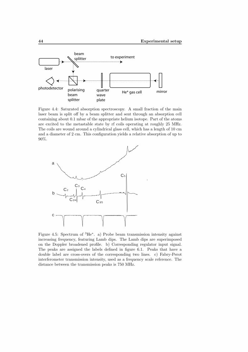
44 Experimental setup
polarisingbeam splitter
beam splitter
laser
mirrorquarterwaveplate
He* gas cellphotodetector
to experiment
Figure 4.4: Saturated absorption spectroscopy. A small fraction of the mainlaser beam is split off by a beam splitter and sent through an absorption cellcontaining about 0.1 mbar of the appropriate helium isotope. Part of the atomsare excited to the metastable state by rf coils operating at roughly 25 MHz.The coils are wound around a cylindrical glass cell, which has a length of 10 cmand a diameter of 2 cm. This configuration yields a relative absorption of up to90%.
C 2
C 3C 4
C 5
C 3/5C 2/4
a
b
c
Figure 4.5: Spectrum of 3He∗. a) Probe beam transmission intensity againstincreasing frequency, featuring Lamb dips. The Lamb dips are superimposedon the Doppler broadened profile. b) Corresponding regulator input signal.The peaks are assigned the labels defined in figure 6.1. Peaks that have adouble label are cross-overs of the corresponding two lines. c) Fabry-Perotinterferometer transmission intensity, used as a frequency scale reference. Thedistance between the transmission peaks is 750 MHz.

4.3 Vacuum system 45
source collimation section
skimmer
Zeeman slower
nozzle
trap slower light
MOT light
MOT light
MOT light
MOT light
absorption imaging light
detection chamber
Figure 4.6: Schematic of the vacuum system. The source is filled with heliumatoms that are excited to the metastable state. The metastables that leave thesource chamber through the nozzle are collimated and slowed before enteringthe trap chamber (see also figure 4.7).
10−4 mbar. Due to several differential pumping stages, the pressure drops whenmoving along the beam line in the direction of the trap chamber. In the trapchamber, the pressure is about 10−10 mbar, a factor of two higher than withoutthe helium load.
Recycling apparatus
3He is rather expensive due to its low relative natural abundance. It is thereforeuseful to recycle it. Only a small fraction of the ground state helium will enterthe collimation section through the nozzle. If the experiment is run with 4He, theremainder of the atoms are pumped away to the atmosphere. When a mixtureof 4He and 3He is used, the exhaust of the source chamber is connected to arecycling system that contains two different types of molecular sieves, cooledby liquid nitrogen, to filter out anything except helium. The turbomolecularpump connected to the source chamber is backed by a scroll pump in stead ofa membrane pump in order to be able to construct a closed circuit.
46 Experimental setup
4.4 Experimental sequence
In our experiments, room temperature helium atoms are cooled to μK temper-atures in a sequence which takes about 20 seconds. During this sequence, theatoms are loaded from a bottle of gas into the vacuum system and excited tothe metastable state by electron bombardment in a high-voltage discharge. Theresulting atomic beam is collimated and deflected, and subsequently slowed bylaser light over a distance of 2.4 meter. The atoms from the slowed beam arecaptured in a magneto-optical trap (MOT). Once the MOT is loaded, the finalcooling stage, consisting of 1D Doppler cooling followed by forced evaporativecooling, brings the atoms into the quantum degenerate regime.
4.4.1 Discharge source
The metastable He atoms are produced in a liquid nitrogen cooled DC dischargesource. The atoms are transferred to the metastable 2 3S1 state (see figure ??) bya discharge current of a few mA, in a narrow tube (the nozzle). About ∼ 0.001%of the atoms are transferred to the metastable state [65]. Only the metastableatoms are cooled by laser light; all other helium atoms can be regarded a sourceof unwanted background pressure.
4.4.2 Collimation and deflection
The beam of metastable atoms enters the collimation section through the nozzleand a skimmer, which provides a first transverse velocity selection. The atomicbeam is collimated and deflected using the curved-wavefront technique [62]. Inshort, cylindrical lenses are used to create a curved wavefront of resonant laserlight with a radius of curvature of 11 m for the horizontal collimation and 15 mfor the vertical beam. Atoms will tend to follow the wave front of the laserbeams and this will result in a collimated beam of metastables. A total amountof ∼ 190 mW of 1083 nm light is sent into the collimation section. Collimationin the vertical plane takes place over a distance of 19 cm. In the horizontalplane, collimation in the first 9.5 cm is followed by deflection over an angle ofabout 1o. The beam of metastables is thus bent around a knife edge which ispositioned such that it blocks the beam of ground state atoms. In this way,there is no direct line from the source to the trap chamber. Therefore, when thecollimation light is switched off, hardly any atoms will enter the trap chamberand affect the trapped cloud. This deflection scheme increases the lifetime of
4.4 Experimental sequence 47
the magnetically trapped cloud by a factor of 5 [63]. Collimation increases theloading rate of the MOT by roughly a factor of 30.
4.4.3 Zeeman slower
The most probable longitudinal velocity of atoms in the collimated atomic beam(∼1100 m/s for 4He∗ and ∼1300 m/s for 3He∗ at liquid nitrogen temperatures)is too high to be able to capture the atoms in the MOT. Therefore, the Zeemanslowing technique is used to slow down atoms to below the MOT’s capture veloc-ity (∼50 m/s). A σ+-polarised laser beam2 is sent counter-propagating alongthe path of the atomic beam. The frequency of the light is 250 MHz detunedto the red of the atomic resonance, using an acousto-optical modulator (AOM).The beam has a power of ∼15 mW and has a diameter of 3 cm when it entersthe vacuum setup. It is focused onto the skimmer. The atoms absorb photonsfrom the slower beam that are subsequently emitted in random directions. Thisprocess yields a net force directed against the movement of the atoms. Atomsthat are in resonance at the beginning of the slowing process, however, willexperience a different Doppler shift once they are decelerated by a significantamount. The atoms would become transparent to the light and the slowingprocess would stop. The decreasing Doppler shift is therefore compensated bya Zeeman shift induced by a spatially varying magnetic field. This Zeeman fieldis created by a current-carrying solenoid wound around the vacuum tube. Thenumber of windings per unit length is chosen such that the resulting magneticfield keeps the atoms in resonance with the Zeeman slower beam along the entirelength of the tube.
The force exerted on the atoms in the Zeeman slower is limited by thenumber of photons that are absorbed per unit time. This number depends onthe laser intensity and the lifetime τ of the exited state of the cooling transition.Furthermore, the force depends on the momentum hk of the absorbed photonsand therefore on the transition frequency ω. At laser intensities for which thetransition is saturated, the atoms spend half of the time in the upper state,so we have for the number of absorbed photons per unit time N = 1
2τ . Thedeceleration a of a mass m is then easily found to be:
a =Nhk
m=
hω
2mcτ(4.4)
2σ+-polarised light only induces transitions with Δm = +1 and σ−-polarised light onlywith Δm = −1.
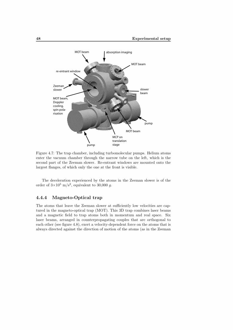
48 Experimental setup
pump
absorption imagingMOT beam
re-entrant window
MOT beam
MOT beam
MOT beam,Dopplercooling,spin pola-risation
pump
MCP on translationstage
slower beam
Zeemanslower
Figure 4.7: The trap chamber, including turbomolecular pumps. Helium atomsenter the vacuum chamber through the narrow tube on the left, which is thesecond part of the Zeeman slower. Re-entrant windows are mounted onto thelargest flanges, of which only the one at the front is visible.
The deceleration experienced by the atoms in the Zeeman slower is of theorder of 3×10⁵ m/s2, equivalent to 30,000 g.
4.4.4 Magneto-Optical trap
The atoms that leave the Zeeman slower at sufficiently low velocities are cap-tured in the magneto-optical trap (MOT). This 3D trap combines laser beamsand a magnetic field to trap atoms both in momentum and real space. Sixlaser beams, arranged in counterpropagating couples that are orthogonal toeach other (see figure 4.8), exert a velocity-dependent force on the atoms that isalways directed against the direction of motion of the atoms (as in the Zeeman

4.4 Experimental sequence 49
Figure 4.8: The magneto-optical trap (MOT). Shown are the two coils thatgenerate a quadrupole magnetic field and the six laser beams that overlap inthe centre of the trap. Arrows indicate the direction of the current flowingthrough the coils and the handedness of the circularly polarised light.
slower). This effect is called optical molasses. The magnetic field, generatedby a set of coils in anti-Helmholtz configuration, yields a space-dependent forcedirected towards the centre of the trap. The field is zero at the centre and thegradient of the field is 19 G/cm along the axis of the trap and half this valuealong the radial direction. The two beams that make up a counterpropagat-ing couple of beams are circularly polarised in the opposite sense: one beamis σ−-polarised and the other one is σ+-polarised and both are detuned to thered from the atomic transition. Because the magnetic field shifts the energy ofthe magnetic sublevels of the atom, and transitions to the different magneticsublevels are polarisation-dependent, either absorption from the σ+ or the σ−
beam is favoured. In this way the atoms will be pushed back towards the centreof the trap, even if they started out with velocities low enough to be outside thecapture range of the optical molasses.
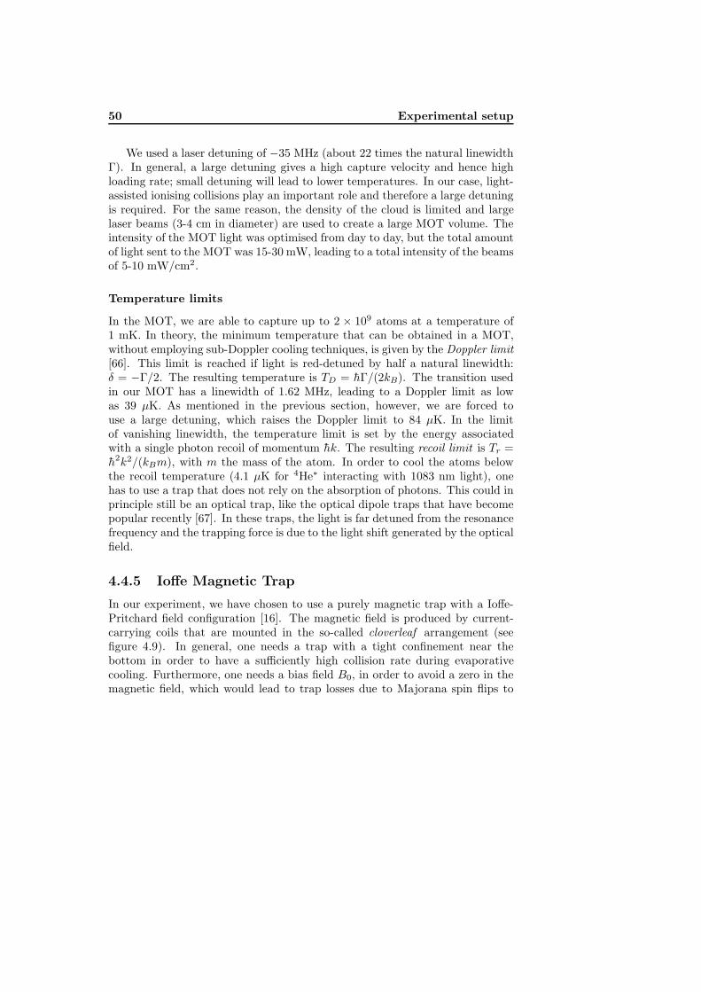
50 Experimental setup
We used a laser detuning of −35 MHz (about 22 times the natural linewidthΓ). In general, a large detuning gives a high capture velocity and hence highloading rate; small detuning will lead to lower temperatures. In our case, light-assisted ionising collisions play an important role and therefore a large detuningis required. For the same reason, the density of the cloud is limited and largelaser beams (3-4 cm in diameter) are used to create a large MOT volume. Theintensity of the MOT light was optimised from day to day, but the total amountof light sent to the MOT was 15-30 mW, leading to a total intensity of the beamsof 5-10 mW/cm2.
Temperature limits
In the MOT, we are able to capture up to 2 × 10⁹ atoms at a temperature of1 mK. In theory, the minimum temperature that can be obtained in a MOT,without employing sub-Doppler cooling techniques, is given by the Doppler limit[66]. This limit is reached if light is red-detuned by half a natural linewidth:δ = −Γ/2. The resulting temperature is TD = hΓ/(2kB). The transition usedin our MOT has a linewidth of 1.62 MHz, leading to a Doppler limit as lowas 39 μK. As mentioned in the previous section, however, we are forced touse a large detuning, which raises the Doppler limit to 84 μK. In the limitof vanishing linewidth, the temperature limit is set by the energy associatedwith a single photon recoil of momentum hk. The resulting recoil limit is Tr =h2k2/(kBm), with m the mass of the atom. In order to cool the atoms belowthe recoil temperature (4.1 μK for 4He∗ interacting with 1083 nm light), onehas to use a trap that does not rely on the absorption of photons. This could inprinciple still be an optical trap, like the optical dipole traps that have becomepopular recently [67]. In these traps, the light is far detuned from the resonancefrequency and the trapping force is due to the light shift generated by the opticalfield.
4.4.5 Ioffe Magnetic Trap
In our experiment, we have chosen to use a purely magnetic trap with a Ioffe-Pritchard field configuration [16]. The magnetic field is produced by current-carrying coils that are mounted in the so-called cloverleaf arrangement (seefigure 4.9). In general, one needs a trap with a tight confinement near thebottom in order to have a sufficiently high collision rate during evaporativecooling. Furthermore, one needs a bias field B0, in order to avoid a zero in themagnetic field, which would lead to trap losses due to Majorana spin flips to
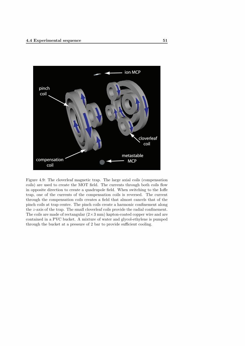
4.4 Experimental sequence 51
metastablemetastable MCP MCP
pinchpinch c coiloil
compompensaensationtion c coiloil
ion MCPion MCP
cloclovererleafleaf c coiloil
Figure 4.9: The cloverleaf magnetic trap. The large axial coils (compensationcoils) are used to create the MOT field. The currents through both coils flowin opposite direction to create a quadrupole field. When switching to the Ioffetrap, one of the currents of the compensation coils is reversed. The currentthrough the compensation coils creates a field that almost cancels that of thepinch coils at trap centre. The pinch coils create a harmonic confinement alongthe z-axis of the trap. The small cloverleaf coils provide the radial confinement.The coils are made of rectangular (2×3 mm) kapton-coated copper wire and arecontained in a PVC bucket. A mixture of water and glycol-ethylene is pumpedthrough the bucket at a pressure of 2 bar to provide sufficient cooling.
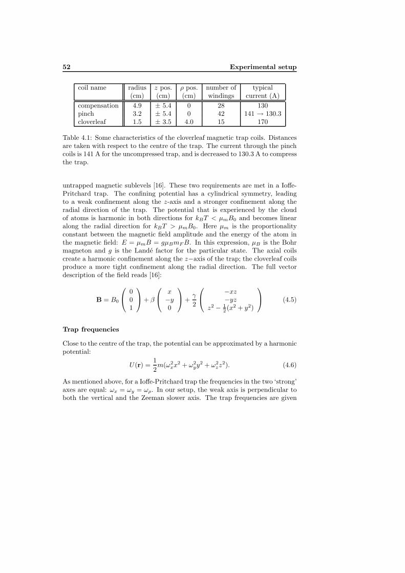
52 Experimental setup
coil name radius z pos. ρ pos. number of typical(cm) (cm) (cm) windings current (A)
compensation 4.9 ± 5.4 0 28 130pinch 3.2 ± 5.4 0 42 141 → 130.3cloverleaf 1.5 ± 3.5 4.0 15 170
Table 4.1: Some characteristics of the cloverleaf magnetic trap coils. Distancesare taken with respect to the centre of the trap. The current through the pinchcoils is 141 A for the uncompressed trap, and is decreased to 130.3 A to compressthe trap.
untrapped magnetic sublevels [16]. These two requirements are met in a Ioffe-Pritchard trap. The confining potential has a cylindrical symmetry, leadingto a weak confinement along the z-axis and a stronger confinement along theradial direction of the trap. The potential that is experienced by the cloudof atoms is harmonic in both directions for kBT < μmB0 and becomes linearalong the radial direction for kBT > μmB0. Here μm is the proportionalityconstant between the magnetic field amplitude and the energy of the atom inthe magnetic field: E = μmB = gμBmFB. In this expression, μB is the Bohrmagneton and g is the Lande factor for the particular state. The axial coilscreate a harmonic confinement along the z−axis of the trap; the cloverleaf coilsproduce a more tight confinement along the radial direction. The full vectordescription of the field reads [16]:
B = B0
⎛⎝ 0
01
⎞⎠+ β
⎛⎝ x
−y0
⎞⎠+
γ
2
⎛⎝ −xz
−yzz2 − 1
2 (x2 + y2)
⎞⎠ (4.5)
Trap frequencies
Close to the centre of the trap, the potential can be approximated by a harmonicpotential:
U(r) =12m(ω2
xx2 + ω2
yy2 + ω2
zz2). (4.6)
As mentioned above, for a Ioffe-Pritchard trap the frequencies in the two ‘strong’axes are equal: ωx = ωy = ωρ. In our setup, the weak axis is perpendicular toboth the vertical and the Zeeman slower axis. The trap frequencies are given

4.4 Experimental sequence 53
by:
ωz =√
2μBγ/m, ωρ =
√2μB
m
(β2
B0− γ
2
), (4.7)
where γ is the axial curvature and β is the radial gradient of the magnetic field,as defined in equation 4.5. B0 is the bias field, which is equal to the field valueat the centre of the trap. The size and therefore density of the cloud dependson the trap frequencies in the following way:
σα =
√kBT
mω2α
, (4.8)
where σα is the rms radius of the cloud in the α-direction.The trap frequencies can be determined in various ways. One can: a) mea-
sure the spatial magnetic field configuration directly, b) calculate the field fromthe coil configuration and measured currents, or c) apply a varying magneticfield in order to induce resonant oscillations of the trapped cloud3. In practice,a model of the cloverleaf trap is used in conjunction with direct field measure-ments and an experimental determination of the most sensitive parameter, B0.The magnetic field minimum can be measured by looking with which RF fre-quency the atoms at the bottom of the trap are resonant (see section 4.4.7).This procedure results in estimated trap frequencies, which provide a frequencyrange in which one can search for resonance behaviour of a trapped cloud witha temperature of a few μK. Radial oscillations are excited by sending an ACcurrent of ∼30 mA through two flatcable coils in Helmholtz configuration. Theaxis of the coils coincides with the weak (z−) axis of the trap. The atoms areexcited at twice the expected radial trap frequency in order to increase the effi-ciency of the process. The same coils, but now in anti-Helmholtz configurationare used to excite the axial mode of the trap. Scanning the frequency resultsin a clear increase in the temperature of the cloud when the driving frequencymatches the trap frequency.
Loading the magnetic trap
To transfer the atoms efficiently from the MOT into the magnetic trap, min-imising losses and heating, the shape of the trap should match the shape of the
3In principle, the size of the thermal cloud in the trap and the expansion characteristics ofthe BEC would also provide information on the trap parameters, but it is difficult to measurethe trap frequencies in this way.
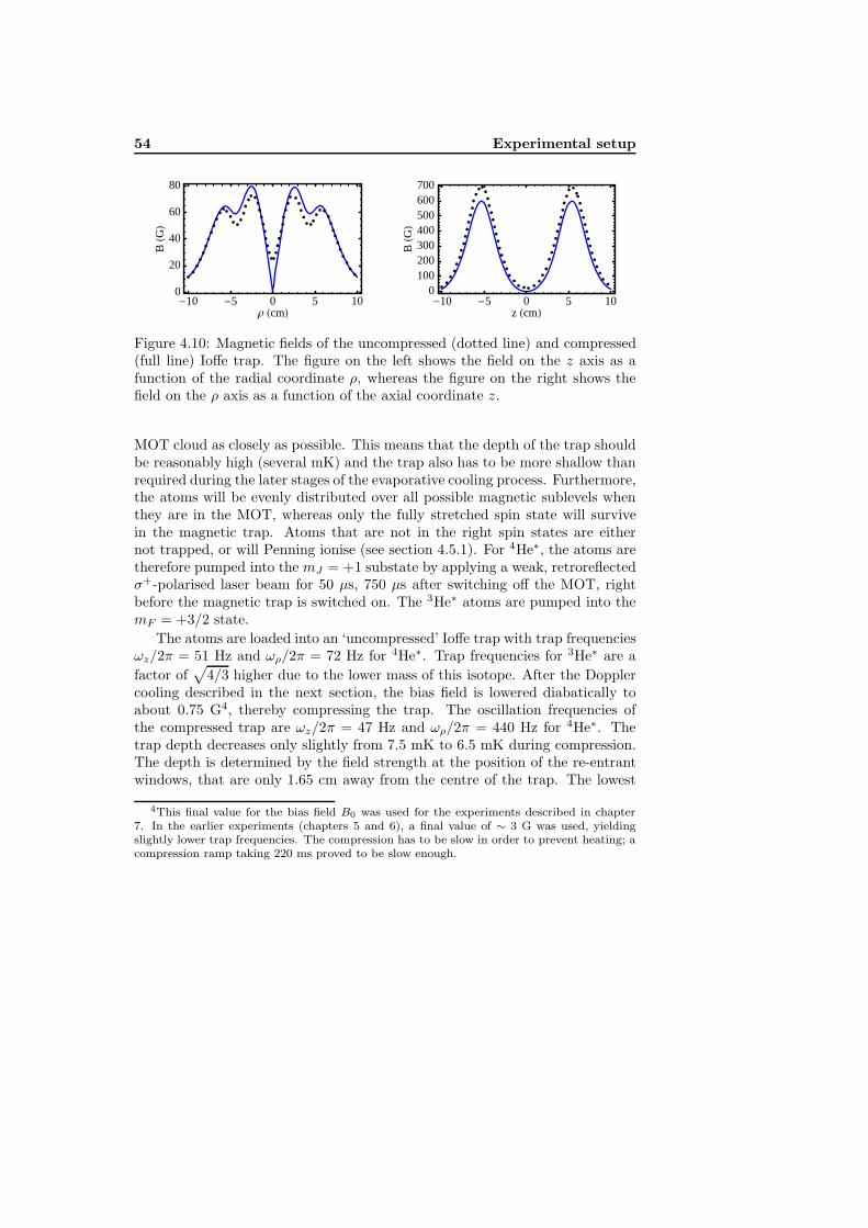
54 Experimental setup
�10 �5 0 5 10Ρ �cm�
0
20
40
60
80
B�G�
�10 �5 0 5 10z �cm�
0100200300400500600700
B�G�
Figure 4.10: Magnetic fields of the uncompressed (dotted line) and compressed(full line) Ioffe trap. The figure on the left shows the field on the z axis as afunction of the radial coordinate ρ, whereas the figure on the right shows thefield on the ρ axis as a function of the axial coordinate z.
MOT cloud as closely as possible. This means that the depth of the trap shouldbe reasonably high (several mK) and the trap also has to be more shallow thanrequired during the later stages of the evaporative cooling process. Furthermore,the atoms will be evenly distributed over all possible magnetic sublevels whenthey are in the MOT, whereas only the fully stretched spin state will survivein the magnetic trap. Atoms that are not in the right spin states are eithernot trapped, or will Penning ionise (see section 4.5.1). For 4He∗, the atoms aretherefore pumped into the mJ = +1 substate by applying a weak, retroreflectedσ+-polarised laser beam for 50 μs, 750 μs after switching off the MOT, rightbefore the magnetic trap is switched on. The 3He∗ atoms are pumped into themF = +3/2 state.
The atoms are loaded into an ‘uncompressed’ Ioffe trap with trap frequenciesωz/2π = 51 Hz and ωρ/2π = 72 Hz for 4He∗. Trap frequencies for 3He∗ are afactor of
√4/3 higher due to the lower mass of this isotope. After the Doppler
cooling described in the next section, the bias field is lowered diabatically toabout 0.75 G4, thereby compressing the trap. The oscillation frequencies ofthe compressed trap are ωz/2π = 47 Hz and ωρ/2π = 440 Hz for 4He∗. Thetrap depth decreases only slightly from 7.5 mK to 6.5 mK during compression.The depth is determined by the field strength at the position of the re-entrantwindows, that are only 1.65 cm away from the centre of the trap. The lowest
4This final value for the bias field B0 was used for the experiments described in chapter7. In the earlier experiments (chapters 5 and 6), a final value of ∼ 3 G was used, yieldingslightly lower trap frequencies. The compression has to be slow in order to prevent heating; acompression ramp taking 220 ms proved to be slow enough.

4.4 Experimental sequence 55
�2
0
2
z �cm�
�2
0
2
Ρ �cm�
0
50
100
150
B �G�
�2
0
2
Ρ �cm�
0
50
1
Figure 4.11: Impression of the magnetic field of the compressed Ioffe trap. Thefield is plotted as a function of the axial (z) and radial (ρ) coordinates. There-entrant windows of the vacuum chamber are shown as planes. Atoms thathit the windows are heated and lost from the trap.

56 Experimental setup
point in the potential barrier created by the trap is located at the intersectionof the z-axis with the window. The trap depths mentioned are calculated asTtrap = 2μBΔB/kB, where ΔB is the difference between the magnetic fieldamplitudes at the window and the centre of the trap.
4.4.6 1D Doppler cooling
After recapturing the atoms in the Ioffe-Pritchard trap, and before compression,we apply another retroreflected σ+-polarised laser beam along the trap axis,cooling the sample to about 0.15 mK. The laser frequency is red-detuned withrespect to the atomic resonance frequency at the centre of the trap. Therefore,atoms will preferentially absorb photons from the beam that is directed againstthe direction of propagation of the atom, thereby cooling the sample along thez-direction. Cooling of the radial velocity component relies on reabsorptionof photons that are spontaneously emitted. This 1D Doppler cooling henceworks only in an optically dense cloud [68]. 1D Doppler cooling is done at arelatively high bias field of 24 Gauss in order to separate the magnetic sublevelsand prevent optical pumping to unwanted Zeeman sublevels. The optimumdetuning is adjusted experimentally (the theoretical optimum is −Γ/2), and theintensity of the beam is roughly one percent of the saturation intensity. It takesabout 2 to 6 seconds before the final temperature is reached, depending on thedensity of the atomic cloud.
4.4.7 Evaporative cooling
Evaporative cooling is a process in which the most energetic atoms escape fromthe trap. The remaining atoms will rethermalise by elastic collisions, yieldinga lower temperature. One can lower the effective trap depth by applying an rfelectromagnetic field which induces spin flips to untrapped states. Dependingon the exact frequency of the rf field, the atoms will be in resonance with thefield when they are in a region of the trap with a specific magnetic field strength.The resonance frequency increases with magnetic field due to the Zeeman effect.Only the most energetic atoms will reach the region of high magnetic field andare lost from the trap. The effective trap depth εt for 4He∗ is given by (neglectinggravity):
εt = hωrf − 2μBB0. (4.9)
Lowering the rf field frequency in time will cool down the sample if the remainingatoms have enough time to rethermalise during the ramp. Most efficient cooling
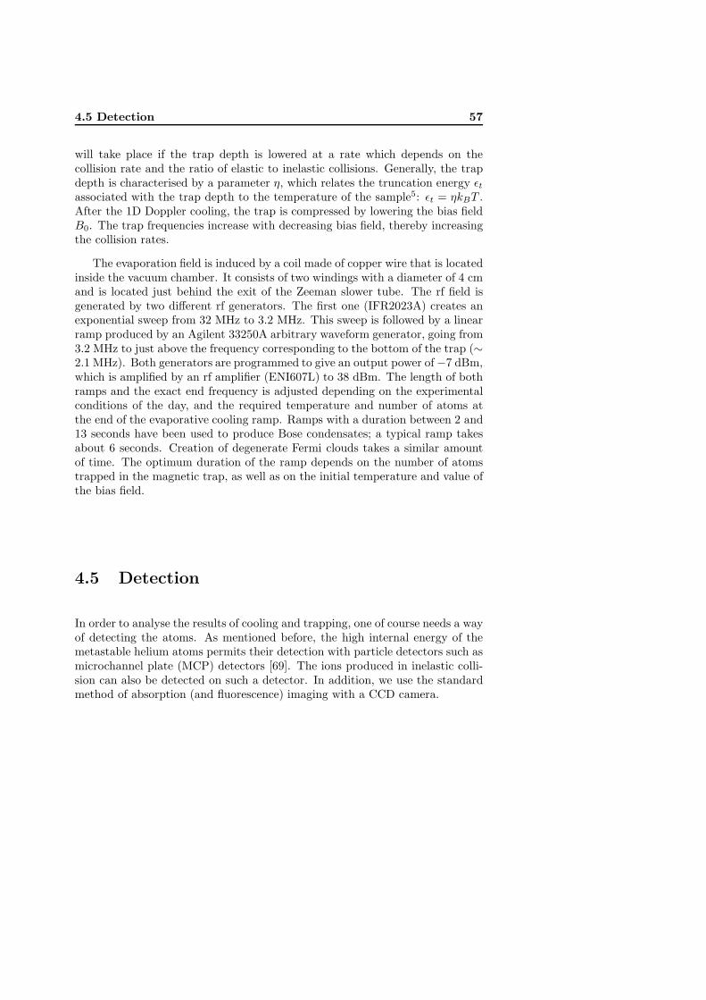
4.5 Detection 57
will take place if the trap depth is lowered at a rate which depends on thecollision rate and the ratio of elastic to inelastic collisions. Generally, the trapdepth is characterised by a parameter η, which relates the truncation energy εtassociated with the trap depth to the temperature of the sample5: εt = ηkBT .After the 1D Doppler cooling, the trap is compressed by lowering the bias fieldB0. The trap frequencies increase with decreasing bias field, thereby increasingthe collision rates.
The evaporation field is induced by a coil made of copper wire that is locatedinside the vacuum chamber. It consists of two windings with a diameter of 4 cmand is located just behind the exit of the Zeeman slower tube. The rf field isgenerated by two different rf generators. The first one (IFR2023A) creates anexponential sweep from 32 MHz to 3.2 MHz. This sweep is followed by a linearramp produced by an Agilent 33250A arbitrary waveform generator, going from3.2 MHz to just above the frequency corresponding to the bottom of the trap (∼2.1 MHz). Both generators are programmed to give an output power of −7 dBm,which is amplified by an rf amplifier (ENI607L) to 38 dBm. The length of bothramps and the exact end frequency is adjusted depending on the experimentalconditions of the day, and the required temperature and number of atoms atthe end of the evaporative cooling ramp. Ramps with a duration between 2 and13 seconds have been used to produce Bose condensates; a typical ramp takesabout 6 seconds. Creation of degenerate Fermi clouds takes a similar amountof time. The optimum duration of the ramp depends on the number of atomstrapped in the magnetic trap, as well as on the initial temperature and value ofthe bias field.
4.5 Detection
In order to analyse the results of cooling and trapping, one of course needs a wayof detecting the atoms. As mentioned before, the high internal energy of themetastable helium atoms permits their detection with particle detectors such asmicrochannel plate (MCP) detectors [69]. The ions produced in inelastic colli-sion can also be detected on such a detector. In addition, we use the standardmethod of absorption (and fluorescence) imaging with a CCD camera.

58 Experimental setup
m = +1
m = 0
3He*4He*
2.1 MHz2.1 MHz 1.4 MHz1.4 MHz
m = -1
m = +3/2
m = +1/2
m = -1/2
m = -3/2
Figure 4.12: Overview of the potentials experienced by the various magneticsubstates of 4He∗ and 3He∗. The atoms are trapped in the m = 1 and m =3/2 states, respectively. These states experience the same potential, but thetransition frequency to untrapped states is always 50% higher for 4He∗. Hence,the 4He∗ atoms can be removed with an rf field which is ramped down from32 MHz to just below 2.1 MHz. The 3He∗ atoms are not removed by the rffield, but sympathetically cooled by collisions with 4He∗.
incomingparticle
MCP 1
MCP 2
metalanode
microchannels
-HV
signal
eleccas cade
tron
Figure 4.13: Schematic of a microchannel plate (MCP) detector in chevronconfiguration, as used in our setup. It consists of two microchannel plates,across which a high voltage is applied. Secondary electrons released from thechannel walls are accelerated by the potential difference. The resulting avalancheof electrons is collected on a metal anode and creates the signal current.

4.5 Detection 59
4.5.1 Single anode MCP’s
For detection of both helium ions and metastable helium atoms, we use twoHamamatsu F4655 microchannel plate detectors. Microchannel plate detectors[70] are particle detectors similar to photomultiplier tubes. They consist of a2-dimensional array of tiny channels (with a diameter of 12 μm in the case ofthe F4655). Particles entering one of the channels of the detector may release anelectron from the channel wall. A potential difference of the order of a kV accel-erates the electron through the microchannel. The accelerated primary electronreleases secondary electrons from the channel wall, creating an avalanche ofelectrons which ends up on the anode of the detector (see figure 4.13). Thecurrent that is generated in this way is a measure of the particle detection rate.Provided that the flux of particles is low and the MCP is used in conjunctionwith a preamplifier/discriminator unit, the detected atoms can be converted tosingle nanosecond pulses, thus allowing atom counting. In our experiments, weused the integrated anode current as a measure of the particle flux. Ion count-ing was only performed for the decay experiment described in chapter 5. Thesensitive area of the MCP’s we used has a diameter of 14.5 mm, and the openarea ratio is 60%.
Ion MCP
Since the internal energy of two 2 3S1 helium atoms (2×19.8 eV) is much largerthan the He ionisation limit of 24.6 eV, binary collisions may lead to Penningionisation (PI) or associative ionisation (AI)
He∗ + He∗ → He + He+ + e− (4.10)
He∗ + He∗ → He+2 + e− (4.11)
In our setup, these ions are detected by an MCP detector of which thefront plate is at negative high voltage, such that the ions are attracted towardthe detector. The detector is located about 8 cm above the trap centre, somedistance away from the vertical. The detection rate is a measure of the numberand density of the atoms in the trap: the number of ions produced per unit timeis given by [71]:
dNion(t)dt
= K
∫n2(r, t)d3r (4.12)
5This parameter should not be confused with the contrast parameter η used in chapters 3and 7.

60 Experimental setup
Figure 4.14: Picture of the trap chamber, with one of the re-entrant windowsremoved. The ‘metastable MCP’, mounted on a translation stage, is clearlyvisible.
The ionisation rate coefficient K depends on the intensity and detuning of thelaser light present in the MOT, as well as on the temperature of the cloud. Therates are also different for 389 nm and 1083 nm trapping light. Experiments havebeen performed in our lab to investingate the influence of the various quantumstates present in MOTs containing 3He∗ and 4He∗ [71, 72].
If both atoms involved in a collision are in the fully stretched spin state(the magnetically trappable states (J,mJ) = (1, 1) and (F,mF ) = (3/2, 3/2)for 4He∗ and 3He∗, respectively), spin is not conserved in the ionising reaction.Ionisation is therefore suppressed by at least four orders of magnitude (in 4He∗),provided that the magnetically trapped cloud is spin polarised in the right way[73].

4.5 Detection 61
Metastable MCP
At 17 cm below the trap, another MCP detector is mounted on a linear feed-through, such that the MCP can be moved horizontally over a distance of twoinches. In this way, the MCP can be moved out of the path of the laser beam thatis used for absorption imaging. For the HBT experiment described in chapter7, the detector could be moved out of the path that the released cloud of atomstraverse when they are dropped onto the position-sensitive MCP detector. Ingeneral, since neutral atoms are not accelerated toward the detector, they donot have enough kinetic energy to release an electron from the wall of a channelof the MCP. However, because the 19.8 eV internal energy is released in aninelastic collision with the detector surface, the neutral metastables generatecan be detected with microchannel plate detectors.
Both MCP detectors are used in the daily alignment procedure. Every real-isation of a MOT is detected on the detector. From the time-of-flight signal(TOF) the temperature can be deduced as well as a relative number of atoms.Calibration of the detector using information from absorption imaging providesan absolute number of atoms. Examples of TOF signals produced by clouds ofvarious temperatures are shown in figure 4.15.
Signal processing
The signal from the MCP is amplified by a factor of 103 using three operationalamplifiers, and a low-pass filter is used to suppress the high-frequency noise. Thesignal is subsequently monitored on a Tektronix TDS210 oscilloscope, which isread out from the GPIB port. The resulting TOF data are fitted to a modelusing the Mathematica software package.
Fit functions
In contrast with the previous trap chamber in our lab, described in the thesesof Tol and Herschbach [63, 74], there are no geometrical constraints involvedin the calculation of the TOF fit functions for the detectors mentioned above.Geometrical constraints are present, though, for the position-sensitive detectordescribed in the next section. This is not obvious at first sight, since there isa direct line of sight from the trapped cloud to all points on the detector. Thereleased atoms, however, will follow a parabolic trajectory: the vertical velocityacquired by gravity is very low at the beginning and the atoms will travel theirmain distance in the horizontal plane while they are still between the re-entrantwindows.

62 Experimental setup
170 180 190 200 210time �ms�
20
40
60
80
100
He�
flux�a
rb.u
nits�
Figure 4.15: Time-of-flight signals recorded on the MCP located 17 cm below thetrap. The end frequency of the evaporative cooling ramp was varied to producesamples ranging from clouds consisting of purely thermal atoms (the broadestcurve), via a bimodal distribution to a (quasi) pure BEC (the narrowest curve).
0 50 100 150 200 250 300time �ms�
0
5
10
15
20
25
30
He�
flux�a
rb.u
nits�
Figure 4.16: Time-of-flight (TOF) curves at various temperatures, assuminga Maxwell-Boltzmann thermal velocity distribution in the trap. From left toright: MOT (1 mK, dotted line), Doppler-cooled Ioffe (120 μK, dashed line) andevaporatively cooled cloud (1 μK, solid line, scaled down by a factor thousand).

4.5 Detection 63
170 180 190 200 210time �ms�
0
5
10
15
20
25
30
35
He�
flux�a
rb.u
nits�
Figure 4.17: Time-of-flight (TOF) curves at 1 μK: bosons (dashed line), fermions(dotted line) and distinguishable particles (solid line). For all curves, the massof 4He∗ is used. The differences between the curves are therefore entirely dueto the different quantum statistics.
140 160 180 200 220time �ms�
0.0
0.5
1.0
1.5
2.0
2.5
He�
flux�a
rb.u
nits�
Figure 4.18: Time-of-flight (TOF) curves at 5 μK for 4He∗ (solid line) and 3He∗
(dotted line). A Maxwell-Boltzmann velocity distribution is assumed in thetrap. The difference in the curves in this plot is therefore due to the differentmasses of the two isotopes.

64 Experimental setup
For the ‘metastable’ MCP, analytical expressions for the expected TOF sig-nal can be derived for both thermal and degenerate clouds of 3He∗ and 4He∗.The model assumes negligible size of the cloud in the trap, as well as adiabaticswitch-off of the trap.
For thermal 4He∗, the initial velocity distribution of the atoms in the trap is aBose-Einstein distribution. For temperatures well above the critical temperatureTC , this distribution converges to the classical Maxwell-Boltzmann distribution.The normalised flux on the detector Φ is given by:
Φ(t) =1
g3(z)g√
2πσx
t2 + t202t
×(g5/2
[z exp
(− x2
0
2σ2x
)]− g5/2
[z exp
(−x
20 +R2
2σ2x
)]), (4.13)
with:
σx =
√kBT
mt (4.14)
x0 = h− gt2
2. (4.15)
In these expressions, t is the time after the atoms are released, g is thegravitational acceleration, and t0 is the arrival time of atoms with zero initialvelocity (t0 =
√2h/g, where h is vertical distance from the trap to the detector).
Furthermore, R is the radius of the detector, and z = exp [μ/(kBT )], where μis the chemical potential, which is defined such that it is large and negative athigh temperatures and reaches zero at TC . gα(x) =
∑∞ρ=1 x
ρ/ρα is the so-calledBose-Einstein function. Examples of flux functions corresponding to variousstages in the cooling process are shown in figure 4.16.
For the fermionic isotope, 3He∗, the flux function is very similar; one onlyhas to replace each function gα(x) by fα(x) = −gα(−x). The effect of thedifferent quantum statistics on the flux function is illustrated in figure 4.17.The influence on the TOF signal of the smaller mass of 3He∗ is shown in figure4.18.
Expansion of Bose-Einstein condensates is entirely different from that ofthermal clouds (see also section 2.2.2). The resulting normalised flux functionis given by the following expression, assuming that the entire BEC is detectedon the MCP:

4.5 Detection 65
Φ(t) =1516g
√m
2μt2 + t20
2t2Re
⎡⎣√
1 − m
2μ
(gt2 − t20
2t
)2⎤⎦
4
(4.16)
In our experiment, we have the problem that when the condensate reachesthe detector, the condensate is slightly larger than the surface area of the MCP.A numerical flux function can be used to model the TOF signal that resultsfrom this situation. However, one has to know the exact location of the centreof the BEC with respect to the detector. This is very hard. We found that theexpansion of the BEC as well as the direction in which the BEC moves during theexpansion was not as expected from the assumption that the trap was switchedoff adiabatically fast. Therefore, the chemical potential that results from a fitwith equation 4.16 does not give the correct number of atoms in the trap. Thechemical potential is overestimated, since the expansion in the radial direction isfaster than expected from theory. Furthermore, we see effects of local saturationof the MCP due to the relatively high density of the BEC. This is why we couldgive only upper and lower limits for the number of atoms in the BEC (see alsochapter 5).
4.5.2 Position-sensitive MCP
The Hanbury Brown-Twiss effect was observed using a position-sensitive MCPdetector, normally used by the cold helium group of the Institute d’Optiquein Orsay [75]. The MCP consists of a double stack of microchannel plates inchevron configuration, with a diameter of 8 cm. Underneath the plates, a delayline anode is installed, which introduces the position sensitivity of the system.The anode consists of a metallic plate with two wires wound around it as heliceswith orthogonally oriented axes. The axes of the delay lines constitute the x-and y-axes of the detector.
A signal consisting of secondary electrons falling onto the delay line is splitinto two pairs of pulses that move toward the four ends of the delay lines. Thearrival time of each pulse can be used to calculate the origin of each set of pulses.Each pulse propagates through the wires with a speed of about one third of thespeed of light. The length of the wires is such that the propagation time of thepulses through the wire is not negligible compared to the time resolution of therecording device. Hence the name delay line. In practice, the electron cloudemerging from the microchannel plate will hit the delay line at several spots.
Due to dispersion of the signal in the wires, the pulses emanating from thedifferent wires will overlap when the pulses exit the wire and are recorded by

66 Experimental setup
Figure 4.19: The position-sensitive MCP from the Orsay group. The pictureshows the MCP when it was mounted in a vacuum chamber that was connectedunderneath our trap chamber for the experiments described in chapter 7.
the discriminator. The recorded arrival time is the centre of gravity of all thesecontributions to the signal. The resolution of the detector is therefore not lim-ited to the density of wires of the anode; sub-wire resolution is possible. Thearrival times of the pulses are recorded using a constant fraction discriminatorin conjunction with a time-to-digital converter. The constant fraction discrim-inator converts the analog pulse to a digital NIM pulse, using a smart schemeto prevent that the time stamp attributed to the pulse depends on the heightof the pulse (as would be the case for a leading edge discriminator). The time-to-digital converter (TDC) writes the arrival times of the digital pulses to amemory.

4.5 Detection 67
Detector characteristics
In order to observe bunching or antibunching of the ultracold helium atoms,one needs of course a sufficient signal to noise ratio. This ratio depends on thedetection efficiency, detection rate and resolution of the detector.
Exact knowledge of the detection efficiency of the detector is not of primeimportance for the experiment described in chapter 7. As long as the efficiencyof detecting an atom is not dependent on the detection of a second atom nearbyin time or space (due to saturation effects, for example), the observed paircorrelation function is not affected by the detection efficiency. The signal tonoise ratio that can be obtained for a sample of given size and temperature,however, does depend on the detection efficiency.
The detection efficiency of the MCP detector depends on two factors. Thefirst is the probability for a particle to trigger the electron amplification process.This probability is called the quantum efficiency of the detector and dependson the open area ratio of the microchannel plate (60 %) and the nature ofthe particles (such as their internal and kinetic energy). The energy requiredto extract a primary electron from the surface of the microchannel plate is ofthe order of 3 eV, much lower than the internal energy of the metastable state(19 eV). Still, the detection efficiency of microchannel plates for He∗ varies alot and is estimated to be only 25±15% [76, 63].
If one uses the MCP in counting mode, a second contribution to the detectionefficiency arises due to the pulse-height distribution of the generated pulses. Theconstant fraction discriminator has a threshold value that should be below theamplitude of a true pulse and above the noise amplitude. Because the gaintends to vary over the surface of the MCP, the threshold value was found to beabove the pulse amplitude of the smallest pulses. This resulted in a electronicdetectivity of about 77%.
The processes described above account for a reduction of the number ofdetected particles. The reverse is also possible: electronic noise due to echos inthe delay detection system can actually produce counts that are not connectedto detected particles. These counts amount to only 2% of the total signal, butfor delays below 300 ns they constitute 60% of the signal. This is why in theconstruction of the pair correlation function a dead time of the detector of 300 nsis assumed [75].

68 Experimental setup
Reconstruction of arrival time and position
Once the signals from the four ends of the delay line and the front and rear endof the microchannel plate itself are recorded, they can be used to reconstruct thearrival of the atoms that produced the signals. Five time stamps are used foreach atom, called x1, x2, y1, y2 and t. The x and y values are the time stampsrecorded from the two ends of the delay line along the respective directions. t isthe arrival time of the atom as given by the microchannel plate. Only three ofthese times are needed to reconstruct the arrival time and position of the atom,the remaining two are used as a consistency check.
From the values of x1 and x2 and the velocity vc of the charge inside thewire, the position x of the detected atom is simply given by:
x = (x1 − x2) × vc (4.17)
and likewise for the y-coordinate.There is a small probability that not all of the four delay line pulses that
are created by a single atom have an amplitude that is above the discriminatorthreshold. The maximum number of atoms that can be reconstructed will beequal to the smallest number of signals recorded by each of the four individualchannels, Nmin. Comparing the number of successfully reconstructed atoms toNmin gives therefore a measure of the reconstruction efficiency, which is deter-mined to be 93% for cold clouds around 1 μK [75].
Resolution
The resolution of the detector directly influences the pair correlation functionthat is measured. It determines the height or depth of the bunching and anti-bunching signal respectively (see also figure 3.2). Secondly, the correlationlength that is observed is the convolution of the real correlation length and thedetector resolution along the relevant direction. Along the vertical direction,the effective spatial resolution can be calculated by multiplying the effectivedead time of the detector by the velocity of the atoms at the time of arrival(3.5 m/s). The effective dead time is the sum of the noise-induced dead timeof 300 ns and the dead time due to the reconstruction of atoms6. This yields aresolution of ∼1 μm.
6This dead time is due to the fact that if two atoms are detected within a certain timespan (∼85 ns), the reconstruction process cannot discern which signal belongs to which atomand neither atom is reconstructed.
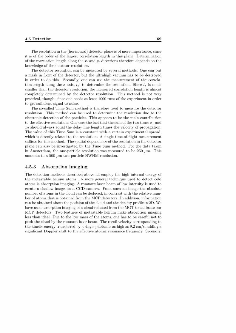
4.5 Detection 69
The resolution in the (horizontal) detector plane is of more importance, sinceit is of the order of the largest correlation length in this plane. Determinationof the correlation length along the x- and y- directions therefore depends on theknowledge of the detector resolution.
The detector resolution can be measured by several methods. One can puta mask in front of the detector, but the ultrahigh vacuum has to be destroyedin order to do this. Secondly, one can use the measurement of the correla-tion length along the x-axis, lx, to determine the resolution. Since lx is muchsmaller than the detector resolution, the measured correlation length is almostcompletely determined by the detector resolution. This method is not verypractical, though, since one needs at least 1000 runs of the experiment in orderto get sufficient signal to noise.
The so-called Time Sum method is therefore used to measure the detectorresolution. This method can be used to determine the resolution due to theelectronic detection of the particles. This appears to be the main contributionto the effective resolution. One uses the fact that the sum of the two times x1 andx2 should always equal the delay line length times the velocity of propagation.The value of this Time Sum is a constant with a certain experimental spread,which is directly related to the resolution. A single time-of-flight measurementsuffices for this method. The spatial dependence of the resolution in the detectorplane can also be investigated by the Time Sum method. For the data takenin Amsterdam, the one-particle resolution was measured to be 250 μm. Thisamounts to a 500 μm two-particle HWHM resolution.
4.5.3 Absorption imaging
The detection methods described above all employ the high internal energy ofthe metastable helium atoms. A more general technique used to detect coldatoms is absorption imaging. A resonant laser beam of low intensity is used tocreate a shadow image on a CCD camera. From such an image the absolutenumber of atoms in the cloud can be deduced, in contrast with the relative num-ber of atoms that is obtained from the MCP detectors. In addition, informationcan be obtained about the position of the cloud and the density profile in 2D. Wehave used absorption imaging of a cloud released from the MOT to calibrate ourMCP detectors. Two features of metastable helium make absorption imagingless than ideal. Due to the low mass of the atoms, one has to be careful not topush the cloud by the resonant laser beam. The recoil velocity corresponding tothe kinetic energy transferred by a single photon is as high as 9.2 cm/s, adding asignificant Doppler shift to the effective atomic resonance frequency. Secondly,

70 Experimental setup
conventional CCD chips have a very low quantum efficiency at the wavelengthof 1083 nm, thus limiting the signal to noise ratio of the absorption images.Presently, cameras based on new materials, such as InGaAs, that have a higherquantum detection efficiency for infrared photons are becoming available.
Absorption
For absorption imaging, the 2 3S1 to 2 3P2 transition is driven using linearlypolarised light. The intensity I of a laser beam travelling along the x-directionthrough an atomic cloud will decrease at a rate which is given by the atomicabsorption rate times the density of the cloud [74]:
dIdx
= −Γ2hω
I/Is1 + I/Is + 4(Δ/Γ)2
· n(x, y, z), (4.18)
where Γ/2π is the FWHM natural linewidth of the transition, Δ/2π is thedetuning from atomic resonance and IS is the saturation intensity of the tran-sition (IS = (17/10) · 0.167 mW/cm2 for a linearly polarised probe laser induc-ing a steady state polarisation of 4He∗ atoms. Unpolarised atoms yield IS =(18/10) · 0.167 mW/cm2, irrespective of the probe polarisation [63, 74]). Thisequation, however, is an approximation assuming negligible linewidth of theprobe laser, as well as negligible width of the velocity distribution of the atoms.Whereas the linewidth of the probe laser of ∼0.5 MHz can be considered negli-gible with respect to the natural linewidth of 1.6 MHz, Doppler broadening cannot be neglected. If the probe intensity used is much smaller than the saturationintensity, the relative transmission can be shown to be given by:
I(x, y, z)I(−∞, y, z)
= exp(−Γ
2hω
Is[1 + 4(Δ/Γ)2]
∫ x
−∞n(x, y, z)dx
). (4.19)
If we want to add the temperature-dependent Doppler broadening, the factor1/[1 + 4(Δ/Γ)2] has to be replaced by a function χ(T ):
χ(T ) =√
m
2πkBT
∫ ∞
−∞
exp[−mv2/(2kBT )]1 + 4[(Δ − kv)/Γ]2
dv. (4.20)
In order to determine the ratio between the incoming and outgoing inten-sities, we take three pictures. A background picture without cloud and probebeam, a probe picture without the cloud present, and an absorption picturewith both probe beam and cloud. The transmittance is then given by:
Iout(y, z)Iin(y, z)
=Iabs(y, z) − Ibgr(y, z)Iprb(y, z) − Ibgr(y, z)
(4.21)

4.5 Detection 71
Fit functions
The density profile of a thermal cloud is well approximated by a Gaussian shape.The function that is used to fit the absorption pictures is therefore given by:
Iout(y, z)Iin(y, z)
= exp[−hωΓ
21I ′s
Nth
2πσyσzexp(− (y − y0)2
2σy2
)exp(− (z − z0)2
2σz2
)],
(4.22)where I ′s is the effective saturation intensity as defined in the thesis of Tol [63]and depends on the polarisation of both the light and the atoms. The fit functioncontains five parameters: the coordinates of the centre of the cloud (y0, z0), therms radii σy and σz and, most importantly, the number of atoms N .
The density distribution of a Bose-Einstein condensate has the shape of aninverted parabola (see section 2.2.2). The corresponding fit function is givenby:
Iout(y, z)Iin(y, z)
= exp
⎛⎝− 5NChωΓ
4πRyRzI ′sRe
[1 −(y − y0Ry
)2
−(z − z0Rz
)2]3/2
⎞⎠ ,
(4.23)where Ry and Rz are the Thomas-Fermi radii of the condensate.
Images of clouds with both a condensed and a thermal component are fittedwith a sum of the two functions given above. An example of such a bimodal fitis shown in figure 4.20.
Probe light
We use a 50 μs pulse of probe light with an intensity of Is/10, meaning thatwe are in the low-intensity limit and the pulse is too short to induce significantpushing of the atoms. In order to produce this short pulse, we first detune theprobe laser by 80 MHz en then send the light through an AOM. When switchedon by a TTL signal, the AOM puts the light back to resonance and deflects thelight over a small angle, such that it overlaps with the cloud. In figure 4.21,a series of absorption images, taken after various expansion times, shows theanisotropic expansion of the Bose-Einstein condensate.
Effect of magnetic fields
If the cloud is imaged in a non-uniform magnetic field, the effective resonancefrequency of the atom varies in space. This yields a spatially varying refractive

72 Experimental setup
index, which causes lensing effects. A similar effect occurs for non-resonantlight and high atomic densities. Imaging the cloud while it is in the magnetictrap is therefore only reliable if the cloud is so small that the magnetic fieldof the trap does not vary significantly over the extension of the cloud. Theresolution of our imaging system appeared insufficient to allow in-situ imagingof the condensate, but we were able to take pictures of the expanding condensate,after it was released from the trap. In general, one has to take care that themagnetic field of the trap has disappeared before the image is taken. Thisrequirement especially causes problems in imaging the MOT cloud, since theexpansion of a cloud released from the MOT occurs on the same timescale asthe decay of eddy currents when the trap is switched off. The design of our newcloverleaf magnetic trap appeared to be such that optical imaging of the MOTcloud during expansion was hampered by the long decay time of the magneticfield (a few ms).
MCP calibration
The Hamamatsu MCP’s were calibrated by comparing the number of atomsin the MOT as deduced from absorption imaging to the integral of the TOFsignal of the same cloud on the MCP. One has to correct for the fact that only acertain fraction f of the atoms will reach the MCP. This fraction is temperature-dependent. The calibration factor C is given by the following expression:
N =NMCP
f=
1fC
∫V (t)dt, (4.24)
where N is the number of trapped atoms, NMCP the number of atoms detectedon the MCP and V (t) the signal recorded on the oscilloscope. Since the gain ofthe MCP depends on the supply voltage, C is a function of this voltage.
Camera
The absorption images were taken with a Hamamatsu C4880 CCD camera usinga standard Frame Grabber card. The CCD chip consists of 512×512 squarepixels of 24×24 μm. The quantum efficiency of the chip for detection of 1083 nmlight is 1.5%.

4.5 Detection 73
-0.15 -0.10 -0.05 0.00 0.05 0.10 0.15
-0.15
-0.10
-0.05
0.00
0.05
0.10
0.15
radial (cm)
axia
l (c
m)
Figure 4.20: Plot of the model function that was used to fit a cloud after 19 msof expansion. One can clearly see the elongated Bose condensed part withthe fainter and more isotropic distribution of thermal atoms surrounding it.The shape of the thermal cloud seems slightly anisotropic, which causes someproblems for the temperature determination with the MCP detector.

74 Experimental setup
0.0 0.2 0.4 0.6radial �cm�
0.0
0.1
0.2
0.3
0.4
0.5
0.6
axia
l�cm�
After 0 ms expansion
0.0 0.2 0.4 0.6radial �cm�
0.0
0.1
0.2
0.3
0.4
0.5
0.6
axia
l�cm�
After 10 ms expansion
0.0 0.2 0.4 0.6radial �cm�
0.0
0.1
0.2
0.3
0.4
0.5
0.6
axia
l�cm�
After 30 ms expansion
0.0 0.2 0.4 0.6radial �cm�
0.0
0.1
0.2
0.3
0.4
0.5
0.6
axia
l�cm�
After 50 ms expansion
0.0 0.2 0.4 0.6radial �cm�
0.0
0.1
0.2
0.3
0.4
0.5
0.6
axia
l�cm�
After 80 ms expansion
Figure 4.21: Absorption images of a BEC taken after various expansion times.One can see that the shape of the condensate changes during the expansion.It is cigar shaped in the trap (with the axial direction as the long axis) andtransforms into a pancake, which is in this case viewed from the side.
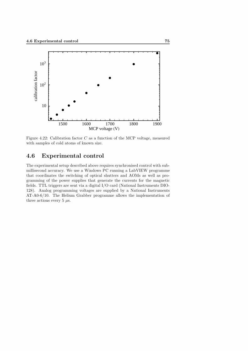
4.6 Experimental control 75
1500 1600 1700 1800 1900MCP voltage �V�
10
102
103
calib
ratio
nfa
ctor
Figure 4.22: Calibration factor C as a function of the MCP voltage, measuredwith samples of cold atoms of known size.
4.6 Experimental control
The experimental setup described above requires synchronised control with sub-millisecond accuracy. We use a Windows PC running a LabVIEW programmethat coordinates the switching of optical shutters and AOMs as well as pro-gramming of the power supplies that generate the currents for the magneticfields. TTL triggers are sent via a digital I/O card (National Instruments DIO-128). Analog programming voltages are supplied by a National InstrumentsAT-A0-6/10. The Helium Grabber programme allows the implementation ofthree actions every 5 μs.

76 Experimental setup

Chapter 5
Metastable heliumBose-Einstein condensatewith a large number ofatoms
(This chapter corresponds to Ref. [77]: Phys. Rev. A. 73, 031603(R) (2006),footnotes are added to provide updates when necessary.)
We have produced a Bose-Einstein condensate of metastable helium (4He∗)containing over 1.5 × 10⁷ atoms, which is a factor of 25 higher than previ-ously achieved. The improved starting conditions for evaporative cooling areobtained by applying one-dimensional Doppler cooling inside a magnetic trap.The same technique is successfully used to cool the spin-polarized fermionicisotope (3He∗), for which thermalizing collisions are highly suppressed. Ourdetection techniques include absorption imaging, time-of-flight measurementson a microchannel plate detector and ion counting to monitor the formationand decay of the condensate.
Ten years after the first experimental realization of Bose-Einstein condensation(BEC) in dilute, weakly interacting atomic systems [9, 10] the field of degeneratequantum gases has developed into a major area of research. For most elements

78 Metastable He BEC with a large number of atoms
it has not yet been possible to produce Bose-Einstein condensates containinglarge numbers of atoms. Only for hydrogen, sodium and rubidium have conden-sates with more than 106 atoms been realized [78]. Large condensates provide abetter signal-to-noise ratio, allow a study of both the collisionless and the hydro-dynamic regime and are especially useful for sympathetic cooling and atom laserapplications. In this realm metastable atoms are of particular interest, offeringalternative detection methods due to their high internal energy. Absorptionimaging is the technique most frequently applied to detect and measure a BEC.Metastable helium (2 3S1 state) is the only species for which detection of thecondensate has been performed using a microchannel plate (MCP) detector [79];the same detector was also used to measure ions produced by Penning ionization(while absorption imaging was not used). In a recent experiment, after pioneer-ing work with metastable neon [48], Schellekens et al. used a position sensitiveMCP detector to observe the Hanbury Brown and Twiss effect both above andbelow the BEC threshold [52]. In the second experiment in which BEC wasrealized with He* [80], optical detection was used and up to 6 × 10⁵ atomscould be condensed. Recently, this group reported a high precision measure-ment of the metastable helium scattering length a, which was performed usinga two-photon dark resonance [18]. The value a = 7.512± 0.005 nm is favorablefor experiments with the fermionic isotope 3He∗. It ensures a stable ultracold4He∗/3He∗ boson-fermion mixture, as the inter-isotope scattering length will belarge and positive [81]. Large numbers of 4He∗ atoms all along to the criti-cal temperature provide an efficient reservoir for sympathetic cooling and willfacilitate the production of degenerate 3He∗ clouds with large numbers of atoms.
In this letter we present an experiment that combines the various detectionmethods used previously [79, 80] and describe the realization of a BEC of 4He∗
containing more than 1.5 × 10⁷ atoms. This large improvement is primarilydue to the application of one-dimensional Doppler cooling inside the magnetictrap rather than three-dimensional Doppler cooling prior to magnetic trapping.Doppler cooling of polarized atoms was originally proposed for atomic hydrogen[82], and has recently been demonstrated for optically dense samples of mag-netically trapped chromium atoms [68]. Compared to the laser cooling methodswe investigated previously [83, 84, 59], this configuration is more efficient andsimple.
The experimental setup is an extended and improved version of our previoussetup [83, 84]. In short, we start with a beam of metastable atoms produced bya liquid-nitrogen cooled dc-discharge source. The atomic beam is collimated,

Metastable He BEC with a large number of atoms 79
deflected and slowed by applying laser beams resonant with the 2 3S1 → 2 3P2
transition at 1083 nm. Typically 2 × 10⁹ atoms are loaded into a magneto-optical trap (MOT) at a temperature of 1 mK. Since our previous experiments[83, 84] we have installed a new ultrahigh vacuum (UHV) chamber and magnetictrap. The coils for our cloverleaf magnetic trap are placed in water-cooled plasticboxes and positioned in re-entrant windows. Inside the UHV chamber two MCPdetectors (Hamamatsu F4655) and an rf-coil are mounted. The first MCP detec-tor is positioned ∼10 cm from the trap center and attracts positively chargedions produced in Penning ionizing collisions: He*+He* → He+ +He(1 1S)+ e−
(or He* + He* → He2+ + e−). These ionization processes are the primary loss
mechanisms in cold clouds of He*. A second (identical) MCP detector shieldedby a grounded grid is positioned 17 cm below the trap center and detects neu-tral He* atoms that fall upon it. This detector is mounted on a translationstage and can be displaced horizontally to allow a vertical laser beam to passthrough the trap center for absorption imaging. Absorption imaging of theMOT cloud determines the number of atoms in the MOT with an accuracy ofabout 20% [83, 84]; this is used to calibrate the He* MCP detector. When theMOT is loaded we switch off all currents and laser beams. In an applied weakmagnetic field we spin-polarize the cloud (atoms are pumped into the m = +1magnetic sublevel) and switch on the currents of the cloverleaf magnetic trap.Typically ∼60% of the atoms is transfered from the MOT into the magnetictrap in this procedure. We operate the cloverleaf trap at a bias magnetic fieldB0=24 G to suppress excitation of depolarizing transitions in the subsequentone-dimensional Doppler cooling stage.
One-dimensional Doppler cooling starts at the same time as the cloverleaf trapis switched on. It is implemented by retroreflecting a weak circularly polarizedlaser beam along the (horizontal) symmetry axis of the magnetic field. Duringthe cooling pulse the temperature decreases reducing the size and increasingthe optical thickness. Cooling in the radial directions relies on reabsorption ofspontaneously emitted red-detuned photons by the optically thick cloud. Otherpossible energy redistribution mechanisms are collisional thermalization andanharmonic mixing. While the collision rate increases from 1.5 s−1 to 20 s−1
during Doppler cooling, anharmonic mixing is negligible in our trap. With alaser detuning of one natural linewidth below the resonance frequency for anatom at rest in the center of the trap and an intensity of 10−3Isat (Isat = 0.17mW/cm2), optimum cooling is realized in 2 seconds. In a separate experi-ment 108 3He∗ atoms were loaded into the magnetic trap and cooled using thesame technique. For identical fermions s-wave collisions are forbidden, while
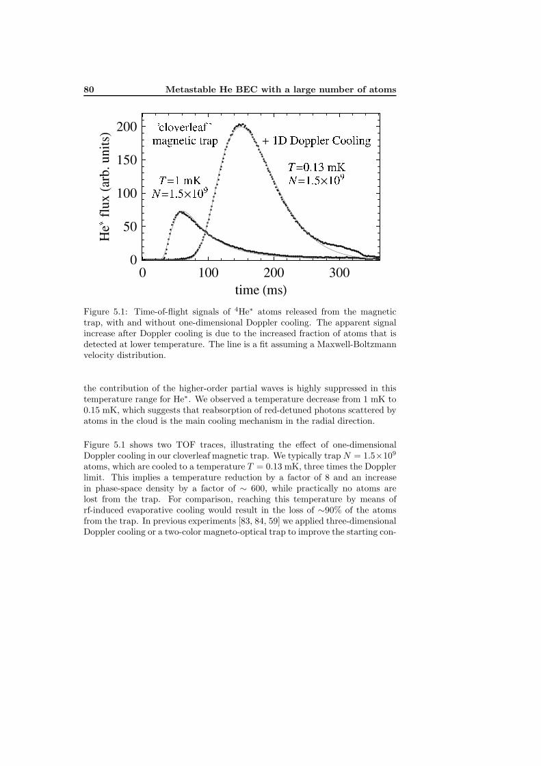
80 Metastable He BEC with a large number of atoms
Figure 5.1: Time-of-flight signals of 4He∗ atoms released from the magnetictrap, with and without one-dimensional Doppler cooling. The apparent signalincrease after Doppler cooling is due to the increased fraction of atoms that isdetected at lower temperature. The line is a fit assuming a Maxwell-Boltzmannvelocity distribution.
the contribution of the higher-order partial waves is highly suppressed in thistemperature range for He∗. We observed a temperature decrease from 1 mK to0.15 mK, which suggests that reabsorption of red-detuned photons scattered byatoms in the cloud is the main cooling mechanism in the radial direction.
Figure 5.1 shows two TOF traces, illustrating the effect of one-dimensionalDoppler cooling in our cloverleaf magnetic trap. We typically trapN = 1.5×10⁹
atoms, which are cooled to a temperature T = 0.13 mK, three times the Dopplerlimit. This implies a temperature reduction by a factor of 8 and an increasein phase-space density by a factor of ∼ 600, while practically no atoms arelost from the trap. For comparison, reaching this temperature by means ofrf-induced evaporative cooling would result in the loss of ∼90% of the atomsfrom the trap. In previous experiments [83, 84, 59] we applied three-dimensionalDoppler cooling or a two-color magneto-optical trap to improve the starting con-

Metastable He BEC with a large number of atoms 81
ditions for evaporative cooling. One-dimensional Doppler cooling provides lowertemperatures, higher phase-space density and is easier to implement. At thispoint the lifetime of the atoms in the magnetic trap is about 3 minutes, limitedby collisions with background gas. To compress the cloud we reduce the biasfield in the trap center to ∼ 3 G in 2.5 seconds, which increases the temperatureto 0.2 mK. The parameters of our magnetic trap then are modest: the axialand radial trap frequencies are ωz/2π = 47 ± 1 Hz and ω⊥/2π = 237 ± 4 Hzrespectively. Higher frequencies are possible but are not required to achieveBEC. Our procedure is similar to previous experiments on evaporative coolingin our group [15]. After compression we cool the gas by rf-induced evaporativecooling in 12 s to BEC, which is achieved at a temperature of ∼ 2 μK. We applya single exponential rf ramp, starting at 50 MHz. The frequency decreases tozero but the ramp is terminated at around 8.4 MHz. Shorter ramps, down to2 s, also produce a condensate, albeit with fewer atoms.
The most sensitive method to detect BEC is TOF analysis of the expandingcloud on the He∗ MCP detector. A typical TOF signal, obtained in a singleshot, is shown in figure 5.2a. The double structure is a combination of theinverted parabola indicating the presence of a BEC released from the harmonictrap and a broad thermal distribution. This signal is used to determine the num-ber of atoms in the condensate as well as in the thermal cloud. In contrast tothe Orsay experiments [79, 52], all atoms stay in the m = +1 sublevel during thetrap switch-off. Applying the MCP calibration, the area under the fitted curvedetermines the number of atoms that have hit the detector. When we consider athermal cloud, this number is only a small fraction of the total number of ther-mal atoms Nth. Therefore the determination of Nth relies upon the measuredtemperature and the MCP calibration. The condensate expansion, determinedby the mean-field interaction energy, is much slower. Thus the condensate willfall completely on the detector sensitive area (diameter of 1.45 cm), allowingus to measure the number of condensed atoms N0 using the MCP calibrationalone. The maximum number of atoms in the condensate deduced in this way is1×107. This number is an underestimate due to MCP saturation effects, whichwill be discussed below. By applying an additional magnetic field pulse we com-pensate small residual field gradients, which otherwise lead to a slight deviationfrom free fall expansion. With stronger field pulses we can also push the cloudtowards the detector and this way realize shorter expansion times. The modelused to fit the time-of-flight signals of the partly condensed clouds (figure 5.2a)is a combination of a thermal part (Bose distribution) and a condensate part(parabolic distribution). The chemical potential μ, the number of atoms and
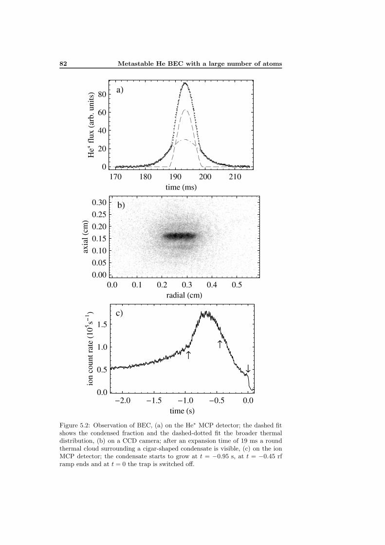
82 Metastable He BEC with a large number of atoms
Figure 5.2: Observation of BEC, (a) on the He∗ MCP detector; the dashed fitshows the condensed fraction and the dashed-dotted fit the broader thermaldistribution, (b) on a CCD camera; after an expansion time of 19 ms a roundthermal cloud surrounding a cigar-shaped condensate is visible, (c) on the ionMCP detector; the condensate starts to grow at t = −0.95 s, at t = −0.45 rframp ends and at t = 0 the trap is switched off.

Metastable He BEC with a large number of atoms 83
the temperature T are the free parameters of the fit; effects of interactions arenot included in the function used for the thermal part. In the Thomas-Fermilimit [2], the chemical potential is given by μ5/2 = 15h2m1/22−5/2N0ω
3a, whereh is Planck’s constant divided by 2π, ω is the geometric mean of the trap fre-quencies, m is the mass of the helium atom and a = 7.512(5) nm [18] is thescattering length. A maximum value of μ extracted from the fit of the TOF sig-nal is ∼ 1.3× 10⁻²⁹ J, which corresponds to 5.1× 10⁷ atoms in the condensate.A possible cause for the discrepancy between the number of atoms determinedfrom the integrated signal and from the measurement of the chemical potentialmay be saturation of the MCP when detecting a falling condensate (peak fluxof ∼ 109 atoms/second); this leads to an underestimation of N0 as well as μ.Another possible cause is distortion of the velocity distribution during the trapswitch-off and influence of remaining magnetic field gradients on the expansionof the cloud. This may lead to an overestimation of μ, and therefore also of N0.
When the MCP detector is shifted horizontally, we can detect the condensateon a CCD camera. A weak (I = 10−1Isat), 50 μs long on-resonance laser pulseis applied to image the shadow of the atoms on the CCD camera for whicha quantum efficiency of ∼ 1.6% is measured at 1083 nm. As expected, thecondensate expands anisotropically while the thermal cloud shows an isotropicexpansion (figure 5.2b). Absolute calibration of the number of atoms at ∼ μKtemperatures could not be performed by optical means. The analysis of theabsorption images, taken between 1 ms and 70 ms after the trap was switchedoff, shows that the condensate expansion deviates from the theoretical predic-tions [17]: it expands faster than expected in the radial direction and slowerin the axial. From these observations we conclude that the expansion of thecloud is influenced by magnetic field gradients during the switch-off of the trap.A difference in the switch-off times of the axial and radial confinement couldcause an additional imbalance in the redistribution of the condensate interac-tion energy between the two directions. This may influence the measurementsof both the chemical potential and the temperature. In order to check if theinteraction energy is conserved, we extract the asymptotic kinetic energy gainedduring the expansion from absorption images of the cloud [85]. In the Thomas-Fermi approximation this so-called release energy should equal the interactionenergy in the trap. We obtain N0 = 4×10⁷ from this analysis assuming that noextra energy is added to (or taken from) the system during the trap switch-off.This is not exactly fulfilled in our case as switching is not fast enough to ensurediabaticity.

84 Metastable He BEC with a large number of atoms
To verify our TOF signal analysis, we plot the chemical potential as a functionof N2/5
0 using data obtained from the MCP measurements (here N0 is the num-ber of condensed atoms measured by integrating the MCP current). The datapoints lie on a straight line which goes through zero with a slope larger thanexpected, meaning that either μ is overestimated or N0 is underestimated. Theformer is supported by the analysis of the absorption images so we correct μ.The corrected data points as well as the theoretical line are presented in theinset of figure 5.3. The plot also shows that the MCP detector saturates, whenthe number of atoms in the condensate exceeds ∼ 106. When we now extractthe number of atoms from the measured chemical potential, after the correctionfor the distortion during the trap switch-off, we find N0 = 1.5 × 10⁷ in ourlargest condensates. This number is still a lower limit, as the analysis assumesthat μ is not affected by saturation of the MCP detector. We, however, measurea reduction in μ when we push the BEC towards the detector, thus increasingthe saturation problem.
With a second MCP detector we observed the growth and decay of our con-densate by counting the ions produced during evaporative cooling. Due to theincrease in density the ion signal increases, although the number of trappedatoms decreases. When BEC sets in, a sharp increase is expected, indicatingthe formation of a dense cloud in the centre of the trap [79]. This is demon-strated in figure 5.2c, which shows the growth of the condensate as well as itsdecay.
The dynamics of formation and decay of the condensate is an interesting aspectthat was discussed and investigated earlier to some extent [87, 88, 89, 90]. Inour group a model was developed describing the decay of the condensate in thepresence of a thermal fraction [86]. The model assumes thermalization to befast compared to the rate of change in thermodynamic variables, so the systemremains in thermal equilibrium during the decay. It was shown that under thisassumption a transfer of atoms should occur from the condensate to the thermalcloud, enhancing the condensate decay rate. To verify this, we performed mea-surements of the BEC lifetime using the TOF signal. Due to the high detectionefficiency it was possible to detect a condensate up to 75 s after it was produced.Results of these measurements are summarised in figure 5.3. We fit the modelto the experimental data for a quasi-pure BEC decay; two- and three-body lossrate constants are used as free parameters. Good agreement with the experi-ment is found for two- and three-body loss rate constants β = 2 × 10⁻¹⁴ cm3
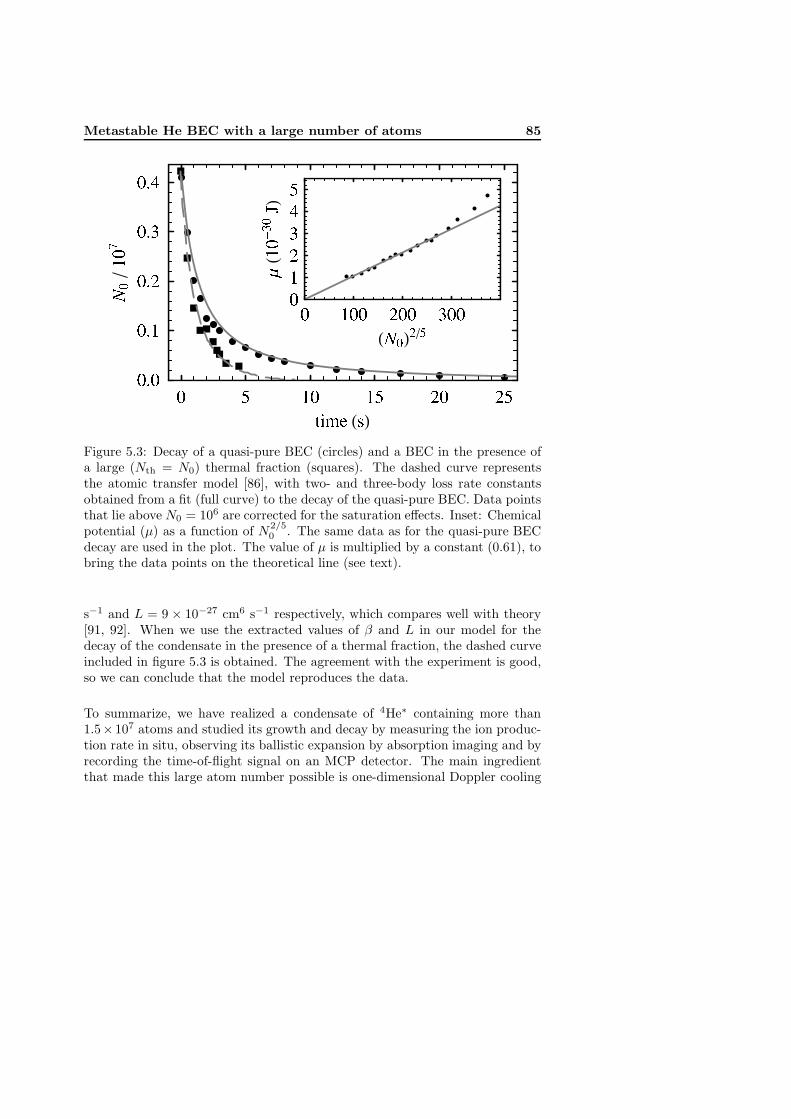
Metastable He BEC with a large number of atoms 85
Figure 5.3: Decay of a quasi-pure BEC (circles) and a BEC in the presence ofa large (Nth = N0) thermal fraction (squares). The dashed curve representsthe atomic transfer model [86], with two- and three-body loss rate constantsobtained from a fit (full curve) to the decay of the quasi-pure BEC. Data pointsthat lie above N0 = 106 are corrected for the saturation effects. Inset: Chemicalpotential (μ) as a function of N2/5
0 . The same data as for the quasi-pure BECdecay are used in the plot. The value of μ is multiplied by a constant (0.61), tobring the data points on the theoretical line (see text).
s−1 and L = 9 × 10⁻²⁷ cm6 s−1 respectively, which compares well with theory[91, 92]. When we use the extracted values of β and L in our model for thedecay of the condensate in the presence of a thermal fraction, the dashed curveincluded in figure 5.3 is obtained. The agreement with the experiment is good,so we can conclude that the model reproduces the data.
To summarize, we have realized a condensate of 4He∗ containing more than1.5×107 atoms and studied its growth and decay by measuring the ion produc-tion rate in situ, observing its ballistic expansion by absorption imaging and byrecording the time-of-flight signal on an MCP detector. The main ingredientthat made this large atom number possible is one-dimensional Doppler cooling

86 Metastable He BEC with a large number of atoms
in the magnetic trap. We demonstrated that this technique can also be appliedto cool spin-polarized helium fermions, where the Pauli principle forbids s-wavecollisions. Combining both isotopes in one setup may allow the observation ofFermi degeneracy in boson-fermion mixtures of metastable atoms1.
1This experiment has been performed and is described in chapter 6.

Chapter 6
Degenerate Bose-Fermimixture of metastableatoms
(This chapter corresponds to Ref. [93]: Phys. Rev. Lett. 97, 080404 (2006),footnotes are added to provide updates when necessary.)
We report the observation of simultaneous quantum degeneracy in a dilutegaseous Bose-Fermi mixture of metastable atoms. Sympathetic cooling of helium-3 (fermion) by helium-4 (boson), both in the lowest triplet state, allows us toproduce ensembles containing more than 106 atoms of each isotope at tempera-tures below 1 μK, and achieve a fermionic degeneracy parameter of T/TF = 0.45.Because of their high internal energy, the detection of individual metastableatoms with subnanosecond time resolution is possible, permitting the study ofbosonic and fermionic quantum gases with unprecedented precision. This maylead to metastable helium becoming the mainstay of quantum atom optics.
The stable fermionic (3He) and bosonic (4He) isotopes of helium (in their groundstate), as well as mixtures of the two, have long exhibited profound quantumproperties in both the liquid and solid phases [94]. More recently, the advent oflaser cooling and trapping techniques heralded the production of Bose-Einsteincondensates (BECs) [9, 10] and the observation of Fermi degeneracy [95, 96] inweakly interacting atomic gases. To date nine different atomic species have been

88 Degenerate Bose-Fermi mixture of metastable atoms
Bose condensed, each exhibiting its own unique features besides many genericphenomena of importance to an increasing number of disciplines.
We can expect that studies of degenerate fermions will have a similar impact,and indeed they have been the object of much study in recent years, culminatingin the detection of superfluidity across the entire crossover region between BECand Bardeen-Cooper-Schriefer pairs [22]. However, only two fermions have sofar been brought to degeneracy in the dilute gaseous phase1: 40K [95] and 6Li[96]. Degenerate atomic Fermi gases have been difficult to realize for two rea-sons: first, evaporative cooling [98] relies upon elastic rethermalizing collisions,which at the temperatures of interest (< 1 mK) are primarily s-wave in natureand are forbidden for identical fermions; and second, the number of fermionicisotopes suitable for laser cooling and trapping is small. Sympathetic cooling[99, 100] overcomes the limit to evaporative cooling by introducing a secondcomponent (spin state, isotope or element) to the gas; thermalization betweenthe two components then allows the mixture as a whole to be cooled.
In 2001, a BEC of helium atoms in the metastable 2 3S1 state (He∗) was realized[79, 80]; more recently we reported the production of a He∗ BEC containing alarge (> 107) number of atoms [77]. A quantum degenerate gas of He∗ is uniquein that the internal energy of the atoms (19.8 eV) is many orders of magnitudelarger than their thermal energy (10−10 eV per atom at 1 μK), allowing efficientsingle atom detection with a high temporal and spatial resolution in the planeof a microchannel plate (MCP) detector [52]. In an unpolarized sample [as isthe case in a magneto-optical trap (MOT)] the internal energy leads to largeloss rates due to Penning (and to a lesser extent associative) ionization [71]:
He∗ + He∗ → He + He+ + e− (and He+2 + e−). (6.1)
These losses are forbidden by angular momentum conservation in a spin-polarizedHe∗ gas, in which all atoms have been transferred into a fully stretched magneticsubstate. Spin-polarization suppresses ionizing losses by 4 orders of magnitudein the case of 4He∗ [80, 101]; it is only this suppression of the loss rate constantto an acceptable value of ∼10−14 cm3/s [80, 77] that has allowed the productionof a BEC in this system [79, 80, 77]. It has been shown that for 4He∗ [101] avery weak spin-dipole magnetic interaction can induce spin flips and mediatePenning ionization; far from being a hindrance, however, the ions produced dur-ing inelastic collisions can allow us to monitor losses non-destructively and in
1Two isotopes of ytterbium have recently been added to the list: 171Yb and 173Yb [97]

Degenerate Bose-Fermi mixture of metastable atoms 89
real time [77, 102].
In 3He∗ the hyperfine interaction splits the 2 3S1 state into an inverted doublet(F = 3/2 and F = 1/2, where F is the total angular momentum quantum num-ber) separated by 6.7 GHz [figure 6.1(a)]. The only magnetically trappable statefor which spin conservation should hold is the |F,MF 〉 = |3/2,+3/2〉 substate(where MF is the projection of F on the quantization axis). Whether or notinteractions would enhance spin-flip processes and the associated loss rate wasunknown, and the prospect of a similarly acceptable level of suppression in thecase of 3He∗ (and indeed between 3He∗ and 4He∗) was an open question beforethis work.
Having realized the capability of producing large BECs of 4He∗ [77], and there-fore large clouds of ultracold 4He∗, we use 4He∗ to sympathetically cool a cloudof 3He∗ into the quantum degenerate regime. In the manner demonstratedpreviously [81], we have adapted our setup [77] to allow the magneto-opticaltrapping of both He∗ isotopes simultaneously. The present configuration trapsa mixture of N3He∗ = 7× 10⁸ and N4He∗ = 1.5× 10⁹ atoms simultaneously at atemperature of ∼1 mK; a complication here is the need for a repumper excitingthe 3He∗ C2 transition, due to the near (−811 MHz) coincidence of the 4He∗
laser cooling and 3He∗ C9 transitions [figure 6.1(a)] [81]. Unable to cool somuch 3He∗ [103], we reduce the number of 3He∗ atoms in the two-isotope MOTto ∼ 107 by either altering the ratio 3He:4He in our helium reservoir or, moresimply, by loading the trap with 3He∗ for a shorter period.
Spin polarization of the mixture to the 3He∗ |3/2,+3/2〉 and 4He∗ |1,+1〉 statesprior to magnetic trapping not only suppresses ionizing losses, but also enhancesthe transfer efficiency of the mixture into the magnetic trap. The applicationof 1D-Doppler cooling along the symmetry axis of our magnetic trap [77] [fig-ure 6.1(b)] reduces the sample temperature to T = 0.13 mK without loss ofatoms, increasing the 4He∗ phase space density by a factor of 600 to ∼ 10−4,greatly enhancing the initial conditions for evaporative cooling. We note atthis point that the application of 1D-Doppler cooling to the 4He∗ componentalready leads to sympathetic cooling of 3He∗, however, the process appears tobe more efficient if we actively cool both components simultaneously. Duringthese experiments the lifetime of a pure sample of either 3He∗ or 4He∗ in themagnetic trap was limited by the background pressure in our ultrahigh vacuumchamber to ∼ 110 s, while the lifetime of the mixture was only slightly shorterat 100 s, indicating that the suppression of Penning ionization during 3He∗-3He∗

90 Degenerate Bose-Fermi mixture of metastable atoms
(a) F J
(c) 3 He*He* 4 He*He*
0
MF MJE
rf
+3/2 +1
2 3P11/2
C9C2 C3 D2
2
3/2
+1/2
1/23/2
B 0
5/2
-1/2
1/23/2
2 3S1
-3/2 -1
3He 4He
Figure 6.1: (a) 3He∗ and 4He∗ energy levels relevant to the magneto-opticaltrapping of He∗ atoms in the 2 3S1 state (F = 3/2 for 3He∗); the cycling tran-sitions (C3 and D2) are indicated (the detunings of the trapping and Zeemanslower (ZS) beams are: δMOT = 40 MHz and δZS = 250 MHz, respectively). Arepumper exciting the C2 transition (δrp = 52 MHz) is applied by simply dou-ble passing our 3He∗ Zeeman slower acousto-optic modulator. (b) Experimen-tal setup for the magneto-optical trapping, magnetic trapping, and detectionof 3He∗ and 4He∗ atoms. A time-of-flight experiment is performed by drop-ping the trapped sample on a microchannel plate detector positioned 17 cmbelow the trap center. (c) Magnetic field dependence of the 3He∗ F = 3/2 and4He∗ J = 1 magnetic substates. Evaporative cooling is performed on the 4He∗
MJ = 1 →M ′J = 0 transition.
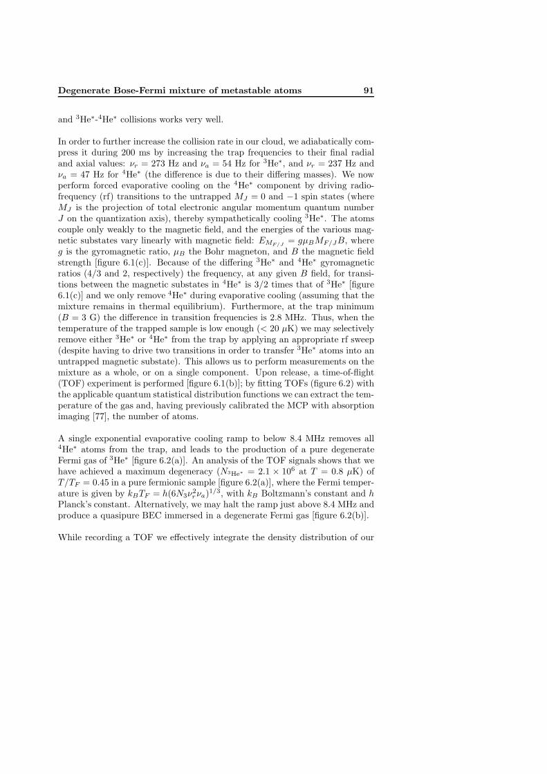
Degenerate Bose-Fermi mixture of metastable atoms 91
and 3He∗-4He∗ collisions works very well.
In order to further increase the collision rate in our cloud, we adiabatically com-press it during 200 ms by increasing the trap frequencies to their final radialand axial values: νr = 273 Hz and νa = 54 Hz for 3He∗, and νr = 237 Hz andνa = 47 Hz for 4He∗ (the difference is due to their differing masses). We nowperform forced evaporative cooling on the 4He∗ component by driving radio-frequency (rf) transitions to the untrapped MJ = 0 and −1 spin states (whereMJ is the projection of total electronic angular momentum quantum numberJ on the quantization axis), thereby sympathetically cooling 3He∗. The atomscouple only weakly to the magnetic field, and the energies of the various mag-netic substates vary linearly with magnetic field: EMF/J
= gμBMF/JB, whereg is the gyromagnetic ratio, μB the Bohr magneton, and B the magnetic fieldstrength [figure 6.1(c)]. Because of the differing 3He∗ and 4He∗ gyromagneticratios (4/3 and 2, respectively) the frequency, at any given B field, for transi-tions between the magnetic substates in 4He∗ is 3/2 times that of 3He∗ [figure6.1(c)] and we only remove 4He∗ during evaporative cooling (assuming that themixture remains in thermal equilibrium). Furthermore, at the trap minimum(B = 3 G) the difference in transition frequencies is 2.8 MHz. Thus, when thetemperature of the trapped sample is low enough (< 20 μK) we may selectivelyremove either 3He∗ or 4He∗ from the trap by applying an appropriate rf sweep(despite having to drive two transitions in order to transfer 3He∗ atoms into anuntrapped magnetic substate). This allows us to perform measurements on themixture as a whole, or on a single component. Upon release, a time-of-flight(TOF) experiment is performed [figure 6.1(b)]; by fitting TOFs (figure 6.2) withthe applicable quantum statistical distribution functions we can extract the tem-perature of the gas and, having previously calibrated the MCP with absorptionimaging [77], the number of atoms.
A single exponential evaporative cooling ramp to below 8.4 MHz removes all4He∗ atoms from the trap, and leads to the production of a pure degenerateFermi gas of 3He∗ [figure 6.2(a)]. An analysis of the TOF signals shows that wehave achieved a maximum degeneracy (N3He∗ = 2.1 × 10⁶ at T = 0.8 μK) ofT/TF = 0.45 in a pure fermionic sample [figure 6.2(a)], where the Fermi temper-ature is given by kBTF = h(6N3ν
2rνa)1/3, with kB Boltzmann’s constant and h
Planck’s constant. Alternatively, we may halt the ramp just above 8.4 MHz andproduce a quasipure BEC immersed in a degenerate Fermi gas [figure 6.2(b)].
While recording a TOF we effectively integrate the density distribution of our

92 Degenerate Bose-Fermi mixture of metastable atoms
250
a
MC
PVo
ltage
mV
MCP
Vol
tage
mV
200
150
100
50
170 180 190 200 210
250
b200
150
100
50
170 180 190 200 210Time of flight ms
Figure 6.2: Time-of-flight spectra for (a) a degenerate Fermi gas of 3He∗ togetherwith the fitted Fermi-Dirac time-of-flight function, from which we conclude thatN3He∗ = 2.1×10⁶ at T = 0.8 μK and T/TF = 0.45; and (b) a degenerate mixtureof N3He∗ = 4.2 × 10⁵ (T/TF = 0.5) and N4He∗ = 1 × 10⁵. The dashed curveis the result of fitting a Fermi-Dirac velocity distribution to the wings, whilethe dot-dashed curve is a fit to a pure Bose-Einstein condensate (showing thecharacteristic inverted parabolic shape).

Degenerate Bose-Fermi mixture of metastable atoms 93
sample over the two dimensions lying in the plane of our MCP detector, andthe small difference between the non-Gaussian distribution of our degenerateFermi gas and the Gaussian distribution of a classical gas becomes even lesspronounced. It is therefore interesting to demonstrate the difference betweenthe TOF of classical gases and quantum gases explicitly, and confirm the resultobtained above. As described by Schreck [23], we repeatedly fit a Gaussiandistribution to a single TOF; before each fit a varying fraction of the TOFpeak center is removed. The population of low energy states is suppressed(enhanced) in a cloud displaying Fermi-Dirac (Bose-Einstein) statistics, and fit-ting a Gaussian distribution to the whole TOF will lead to an overestimation(underestimation) of the cloud size and therefore the temperature of the sample.By fitting only the more ”classical” wings of a TOF these effects are negated,and the fitted temperature should either fall (fermions), rise (bosons), or stayconstant in the case of a classical gas. The high signal-to-noise ratio of ourTOF spectra allows us to see this behavior clearly (figure 6.3). By taking thetemperature from a TOF for which we have removed 1.75 σ0 [where σ0 is theroot-mean-square width of a Gaussian fit to the entire TOF, see figure 6.3(a)],and the number of atoms calculated by integrating the TOF, we again recovera degeneracy parameter of T/TF = 0.5.
It is interesting to note that we have produced degenerate Fermi gases withevaporative cooling ramps as short as 2.5 s (N3He∗ = 4×10⁶ and T/TF = 0.75),signifying that the process of rethermalization is very efficient. At densities of1010 − 1012 atoms/cm3 this indicates a large heteronuclear scattering length.Recently, theory [104] and experiment [18] finally agreed upon the 4He∗-4He∗
scattering length [a44 = 7.64(20) and 7.512(5) nm, respectively]. An extensionto the theory of Przybytek and Jeziorski [104] suggests that the 3He∗-4He∗ scat-tering length should also be very large and positive (a34 = +28.8+3.9
−3.3 nm) [105].Such a large heteronuclear scattering length leads us to expect that losses, inparticular, boson-boson-fermion (BBF) 3-body losses (which scale with a4), willhave a significant impact on the mixture. We can estimate (order of magnitude)the BBF 3-body loss rate constant by using KBBF
3 = 120ha434
√d+ 2/d/(m4
√3)
[106]2, where d is the 3He∗:4He∗ mass ratio, m4 is the 4He∗ mass and we assumethe theoretical value of a34 given above. This gives KBBF
3 ≈ 1.4× 10⁻²⁴ cm6/s,indicating an atom loss rate that is 1− 3 orders of magnitude larger than in thecase of pure 4He∗, and a condensate lifetime (τC) which is significantly shorter
2Equation 3 in [106] has been adapted to take into account the reduced symmetry of theproblem and differing mass factors, and the sin2 factor is assumed to be unity [107].

94 Degenerate Bose-Fermi mixture of metastable atoms
1.10 a
1.05
Fitt
edte
mpe
ratu
reμK 1.00
0.95 0
0.90
0.0 0.5 1.0 1.5 2.00.90
5.25 b 0.85 c5.00 0.804.75 0.754.50 0.70
0.0 0.5 1.0 1.5 2.0 0.0 0.5 1.0 1.5 2. 0Fraction of 0 removed
Figure 6.3: Temperatures obtained by repeatedly fitting 3 time-of-flight spectra(from which increasingly large central fractions are removed) with a classicalMaxwell-Boltzmann distribution: (a) a degenerate 3He∗ Fermi gas (T/TF =0.5), (b) a thermal cloud of 4He∗ atoms with T � TC (a similar plot is observedfor a Fermi gas with T > TF ) and (c) a Bose gas of 4He∗ atoms just above TC ,which adheres to Bose-Einstein statistics.

Degenerate Bose-Fermi mixture of metastable atoms 95
in the degenerate mixture than in the absence of 3He∗. These estimates are inagreement with initial observations that τ (3+4)
C ∼ 0.01 s while τ (4)C ∼ 1 s [77].
Given the large magnitude of a34 and having seen no evidence for a collapseof the mixture, we may further suppose that a34 is positive. This is then thefirst Bose-Fermi system to exhibit boson-fermion and boson-boson interactionswhich are both strong and repulsive. A possible disadvantage, however, maybe that the system is only expected to be sufficiently stable against Penningionization when the atoms are all in the fully stretched magnetic substates,hampering the exploitation of possible Feshbach or optical resonances.
In conclusion, we have successfully produced a degenerate Fermi gas of metastable3He∗ containing a large number of atoms with T/TF = 0.45 and have also seenthat we can produce a degenerate Bose-Fermi mixture of 3He∗ and 4He∗. Thissource of degenerate metastable fermions, bosons, or mixtures of the two, couldform the basis of many sensitive experiments in the area of quantum atomoptics and quantum gases. Of particular interest is the recently realized Han-bury BrownTwiss experiment on an ultracold gas of 4He∗ [52], demonstratingtwo-body correlations (bunching) with neutral atoms (bosons); we now have theideal source to study antibunching in an ultracold Fermi gas of neutral atoms3.The extremely large and positive 3He∗-4He∗ scattering length lends itself to thehitherto unobserved phenomenon of phase separation in a Bose-Fermi mixture[108] and, if the scattering lengths can be tuned only slightly, may allow a studyof p-wave Cooper pairing of identical fermions mediated by density fluctuationsin a bosonic component [109]. Given the naturally large and positive scatter-ing lengths, loading such a mixture into an optical lattice will provide a newplayground for the study of exotic phases and phase transitions [110], includingsupersolidity [111]. The possibility of ion detection as a real-time, nondestruc-tive density determination tool will be very helpful in observing these and otherphenomena. Finally, the ultralow temperatures to which we can now cool bothisotopes will allow unprecedented accuracy in high resolution spectroscopy ofthe helium atom. This could improve the accuracy to which the fine structureconstant is known and may allow, via isotope shift measurements, an accuratemeasurement of the difference in charge radius of the 3He∗ and 4He∗ nucleus[112], challenging nuclear physics calculations.
3This experiment has been performed and is described in chapter 7.

96 Degenerate Bose-Fermi mixture of metastable atoms

Chapter 7
Comparison of the HanburyBrown-Twiss effect forbosons and fermions
(This chapter corresponds to Ref. [113]: Nature 445, 402–405 (2007))
Fifty years ago, Hanbury Brown and Twiss (HBT) discovered photon bunchingin light emitted by a chaotic source [26], highlighting the importance of two-photon correlations [114] and stimulating the development of modern quantumoptics [32]. The quantum interpretation of bunching relies upon the constructiveinterference between amplitudes involving two indistinguishable photons, and itsadditive character is intimately linked to the Bose nature of photons. Advancesin atom cooling and detection have led to the observation and full characterisa-tion of the atomic analogue of the HBT effect with bosonic atoms [48, 52, 49].By contrast, fermions should reveal an antibunching effect (a tendency to avoideach other). Antibunching of fermions is associated with destructive two-particleinterference and is related to the Pauli principle forbidding more than one identi-cal fermion to occupy the same quantum state. Here we report an experimentalcomparison of the fermionic and the bosonic HBT effects realised in the sameapparatus, using two different isotopes of helium: 3He (a fermion) and 4He (aboson). Ordinary attractive or repulsive interactions between atoms are negli-gible; therefore, the contrasting bunching and antibunching behaviour that weobserve can be fully attributed to the different quantum statistics of each atomic

98 HBT effect for bosons and fermions
species. Our result shows how atom-atom correlation measurements can be usedto reveal details in the spatial density [50, 115] or momentum correlations [116]in an atomic ensemble. They also enable the direct observation of phase effectslinked to the quantum statistics of a many-body system, which may facilitatethe study of more exotic situations [43].
Two-particle correlation analysis is an increasingly important method for study-ing complex quantum phases of ultracold atoms [50, 115, 116, 43, 117, 118, 119].It goes back to the discovery, by Hanbury Brown and Twiss [26], that photonsemitted by a chaotic (incoherent) light source tend to be bunched: the jointdetection probability is enhanced, compared to that of statistically independentparticles, when the two detectors are close together. Although the effect is easilyunderstood in the context of classical wave optics [34], it took some time to finda clear quantum interpretation [32, 30]. The explanation relies upon interfer-ence between the quantum amplitude for two particles, emitted from two sourcepoints S1 and S2, to be detected at two detection points D1 and D2 (see figure7.1). For bosons, the two amplitudes 〈D1|S1〉 〈D2|S2〉 and 〈D1|S2〉 〈D2|S1〉 mustbe added, which yields a factor of 2 excess in the joint detection probability,if the two amplitudes have the same phase. The sum over all pairs (S1,S2)of source points washes out the interference, unless the distance between thedetectors is small enough that the phase difference between the amplitudes isless than one radian, or equivalently if the two detectors are separated by a dis-tance less than the coherence length. Study of the joint detection rates versusdetector separation along the i direction then reveals a ‘bump’ whose width liis the coherence length along that axis [26, 52, 27, 41, 42, 54]. For a source sizesi (defined as the half width at e−1/2 of a Gaussian density profile) along the idirection, the bump has a half width at 1/e of li = ht/(2πmsi), where m is themass of the particle, t the time of flight from the source to the detector, and hPlancks constant. This formula is the analogue of the formula li = Lλ/(2πsi)for photons, if λ = h/(mv) is identified with the de Broglie wavelength for par-ticles travelling at velocity v = L/t from the source to the detector.
For indistinguishable fermions, the two-body wave function is antisymmetric,and the two amplitudes must be subtracted, yielding a null probability forjoint detection in the same coherence volume. In the language of particles,it means that two fermions cannot have momenta and positions belonging tothe same elementary cell of phase space. As a result, for fermions the jointdetection rate versus detector separation is expected to exhibit a dip aroundthe null separation. Such a dip for a fermion ensemble must not be confused
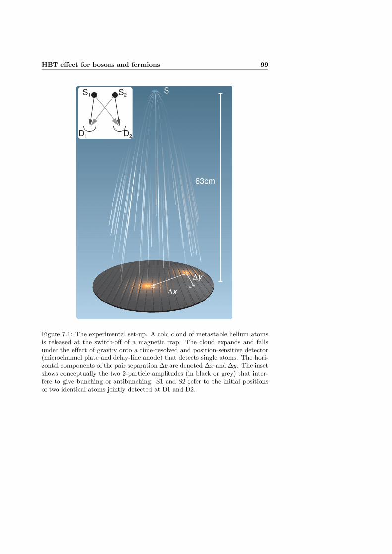
HBT effect for bosons and fermions 99
S
Δx
S1
63cm
Δy
D1 D2
S2
Figure 7.1: The experimental set-up. A cold cloud of metastable helium atomsis released at the switch-off of a magnetic trap. The cloud expands and fallsunder the effect of gravity onto a time-resolved and position-sensitive detector(microchannel plate and delay-line anode) that detects single atoms. The hori-zontal components of the pair separation Δr are denoted Δx and Δy. The insetshows conceptually the two 2-particle amplitudes (in black or grey) that inter-fere to give bunching or antibunching: S1 and S2 refer to the initial positionsof two identical atoms jointly detected at D1 and D2.
100 HBT effect for bosons and fermions
with the antibunching dip that one can observe with a single particle (boson orfermion) quantum state—for example, resonance fluorescence photons emittedby an individual quantum emitter [39]. In contrast to the HBT effect for bosons,the fermion analogue cannot be interpreted by any classical model, either waveor particle, and extensive efforts have been directed towards an experimen-tal demonstration. Experiments have been performed with electrons in solids[44, 45] and in a free beam [46], and with a beam of neutrons [47], but none hasallowed a detailed study and a comparison of the pure fermionic and bosonicHBT effects for an ideal gas. A recent experiment using fermions in an opticallattice [51], however, does permit such a study and is closely related to our work.
Here, we present an experiment in which we study the fermionic HBT effectfor a sample of polarised, metastable 3He atoms (3He∗), and we compare itto the bosonic HBT effect for a sample of polarised, but not Bose condensed,metastable 4He atoms (4He∗) produced in the same apparatus at the same tem-perature. We have combined the position- and time-resolved detector previouslyused [52, 120] for 4He∗, with an apparatus with which ultracold samples of 3He∗
or 4He∗ have recently been produced [93]. Fermions or bosons at thermal equi-librium in a magnetic trap are released onto the detector which counts individualatoms (see figure 7.1) with an efficiency of approximately 10%. The detectorallows us to construct the normalised correlation function g(2)(Δr), that is, theprobability of joint detection at two points separated by Δr, divided by theproduct of the single detection probabilities at each point. Statistically inde-pendent detection events result in a value of 1 for g(2)(Δr). A value larger than1 indicates bunching, while a value less than 1 is evidence of antibunching.
We produce gases of pure 3He∗ or pure 4He∗ by a combination of evapora-tive and sympathetic cooling in an anisotropic magnetic trap (see Methods).Both isotopes are in pure magnetic substates, with nearly identical magneticmoments and therefore nearly identical trapping potentials, so that trappednon-degenerate and non-interacting samples have the same size at the sametemperature. The temperatures of the samples yielding the results of figure 7.2,as measured by the spectrum of flight times to the detector, are 0.53± 0.03 μKand 0.52±0.05 μK for 3He∗ and 4He∗ respectively. The uncertainties correspondto the standard deviation of each ensemble. In a single realization, we typicallyproduce 7 × 10⁴ atoms of both 3He∗ and 4He∗. The atom number permitsan estimate of the Fermi and BEC temperatures of approximately 0.9 μK and0.4 μK, respectively. Consequently, Fermi pressure in the trapped 3He∗ samplehas a negligible (3%) effect on the trap size and repulsive interactions in the
HBT effect for bosons and fermions 101
4He∗ sample have a similarly small effect. The trapped samples are thereforeapproximately Gaussian ellipsoids elongated along the x axis with an r.m.s. sizeof about 110 × 12 × 12 μm3. To release the atoms, we turn off the current inthe trapping coils and atoms fall under the influence of gravity. The detector,placed 63 cm below the trap centre (see figure 7.1), then records the x− y posi-tion and arrival time of each detected atom.
The normalised correlation functions g(2)(0, 0,Δz) along the z (vertical) axis,for 3He∗ and 4He∗ gases at the same temperature, are shown in figure 7.2. Eachcorrelation function is obtained by analysing the data from about 1000 separateclouds for each isotope (see Methods). Results analogous to those of figure 7.2are obtained for correlation functions along the y axis, but the resolution of thedetector in the x−y plane (about 500 μm half width at 1/e for pair separation)broadens the signals. Along the x axis (the long axis of the trapped clouds),the expected widths of the HBT structures are one order of magnitude smallerthan the resolution of the detector and are therefore not resolved.
Figure 7.2 shows clearly the contrasting behaviours of bosons and fermions. Inboth cases we observe a clear departure from statistical independence at smallseparation. Around zero separation, the fermion signal is lower than unity (anti-bunching) while the boson signal is higher (bunching). Since the sizes of the3He∗ and 4He∗ clouds at the same temperature are the same, as are the timesof flight (pure free fall), the ratio of the correlation lengths is expected to beequal to the inverse of the mass ratio, 4/3. The observed ratio of the correlationlengths along the z axis in the data shown is 1.3±0.2. The individual correlationlengths are also in good agreement with the formula lz = ht/(2πmsz). Owingto the finite resolution, the contrast in the signal, which should ideally go to 0or 2 is reduced by a factor of order ten. The amount of contrast reduction isslightly different for bosons and fermions and the ratio should be about 1.5. Themeasured ratio is 2.4± 0.2. This discrepancy has several possible explanations.First, the magnetic field switch-off is not sudden (time scale ∼ 1 ms) and thiscould affect bosons and fermions differently. Second, systematic errors may bepresent in our estimate of the resolution function. The resolution however, doesnot affect the widths of the observed correlation functions along z, and thuswe place the strongest emphasis on this ratio as a test of our understandingof boson and fermion correlations in an ideal gas. More information on uncer-tainties, systematic errors as well as a more complete summary of the data, aregiven in Supplementary Information.

102 HBT effect for bosons and fermions
Separation Δz (mm)
Corre
latio
n g(
2)(Δ
z)
0 1 2 30.9
0.95
1
1
1.05
Figure 7.2: Normalized correlation functions for 4He∗ (bosons) in the upperplot, and 3He∗ (fermions) in the lower plot. Both functions are measured at thesame cloud temperature (0.5 μK), and with identical trap parameters. Errorbars correspond to the root of the number of pairs in each bin. The line is a fitto a Gaussian function. The bosons show a bunching effect, and the fermionsshow anti-bunching. The correlation length for 3He∗ is expected to be 33%larger than that for 4He∗ owing to the smaller mass. We find 1/e values forthe correlation lengths of 0.75± 0.07 mm and 0.56± 0.08 mm for fermions andbosons, respectively.
HBT effect for bosons and fermions 103
Improved detector resolution would allow a more detailed study of the correla-tion function, and is thus highly desirable. The effect of the resolution couldbe circumvented by using a diverging atom lens to demagnify the source [48].According to the formula l = ht/(2πms), a smaller effective source size gives alarger correlation length. We have tried such a scheme by creating an atomiclens with a blue detuned, vertically propagating, laser beam, forcing the atomsaway from its axis (see Methods). The laser waist was not large compared tothe cloud size and therefore our ‘lens’ suffered from strong aberrations, but acrude estimate of the demagnification, neglecting aberrations, gives about 2 inthe x − y plane. Figure 7.3 shows a comparison of g(2)(Δz) for fermions withand without the defocusing lens. We clearly see a greater antibunching depth,consistent with larger correlation lengths in the x − y plane (we have checkedthat ly is indeed increased) and therefore yielding a smaller reduction of thecontrast when convolved with the detector resolution function. As expected,the correlation length in the z direction is unaffected by the lens in the x − yplane. Although our atomic lens was far from ideal, the experiment shows thatit is possible to modify the HBT signal by optical means.
To conclude, we emphasize that we have used samples of neutral atoms at amoderate density in which interactions do not play any significant role. Carewas taken to manipulate bosons and fermions in conditions as similar as possi-ble. Thus the observed differences can be understood as a purely quantum effectassociated with the exchange symmetries of wave functions of indistinguishableparticles.
The possibility of having access to the sign of phase factors in a many-bodywave function opens fascinating perspectives for the investigation of intriguinganalogues of condensed-matter systems, which can now be realized with coldatoms. For instance, one could compare the many-body state of cold fermionsand that of ‘fermionised’ bosons in a one-dimensional sample [121, 122]. Oursuccessful manipulation of the HBT signal by interaction with a laser suggeststhat other lens configurations could allow measurements in position space (byforming an image of the cloud at the detector) or in any combination of momen-tum and spatial coordinates.

104 HBT effect for bosons and fermions
Corre
latio
n g(
2)(Δ
z)
Separation Δz (mm)0 1 2 3
0.95
0.9
1
1.05
Figure 7.3: Effect of demagnifying the source size. We show normalized corre-lation functions along the z (vertical) axis for 3He∗, with (dark squares) andwithout (light circles) a diverging atomic lens in the x − y plane (see text).The dip is deeper with the lens because the increase of the correlation lengthsin the x − y plane leads to less reduction of contrast when convolved with theresolution function in that plane.
Methods
Experimental sequence.Clouds of cold 4He∗ are produced by evaporative cooling of a pure 4He∗ sample,loaded into a Ioffe-Pritchard magnetic trap [77]. The trapped state is 2 3S1,mJ = 1 and the trap frequency values are 47 Hz and 440 Hz, for axial andradial confinement respectively. The bias field is 0.75 G, corresponding to afrequency of 2.1 MHz for a transition between the mJ = 1 and mJ = 0 states atthe bottom of the trap. After evaporative cooling, we keep the radio frequencyevaporation field (‘r.f. knife’) on at constant frequency for 500 ms, then waitfor 100 ms before switching off the trap. In contrast to the experiments of [52],
HBT effect for bosons and fermions 105
atoms are released in a magnetic field sensitive state.
To prepare 3He∗ clouds, we simultaneously load 3He∗ and 4He∗ atoms in themagnetic trap [93]. The trapping state for 3He∗ is 2 3S1, F = 3/2,mF = 3/2,and axial and radial trap frequencies are 54 Hz and 506 Hz—the difference com-pared to 4He∗ is only due to the mass. The two gases are in thermal equilibriumin the trap, so that 3He∗ is sympathetically cooled with 4He∗ during the evap-orative cooling stage. Once the desired temperature is reached, we selectivelyeliminate 4He∗ atoms from the trap using the r.f. knife. The gyromagneticratios for 4He∗ and 3He∗ are 2 and 4/3 respectively, so that the resonant fre-quency of the m = 1 to m = 0 transition for 4He∗ is 3/2 times larger than them = 3/2 to m = 1/2 transition for 3He∗. An r.f. ramp from 3 MHz to 1.9 MHzexpels all the 4He∗ atoms from the trap without affecting 3He∗. We then use thesame trap switch-off procedure to release the 3He∗ atoms (also in a magneticfield-sensitive state) onto the detector. We can apply magnetic field gradientsto check the degree of spin polarisation of either species.
Correlation function.The detailed procedure leading to this correlation is given in [52]. Briefly, weconvert arrival times to z positions and then use the 3-dimensional positionsof each atom to construct a histogram of pair separations Δr in a particularcloud. We then sum the pair distribution histograms for 1000 successive runs atthe same temperature. For separations much larger than the correlation length,this histogram reflects the Gaussian spatial distribution of the cloud. To removethis large scale shape and obtain the normalized correlation function, we dividethe histogram by the autoconvolution of the sum of the 1000 single-particle dis-tributions.
Atom lens experiment.A 300 mW laser beam with an elliptical waist of approximately 100× 150 μm2
propagates vertically through the trap. The laser frequency is detuned by300 GHz from the 2 3S1 to 2 3P2 transition. After turning off the magnetictrap, and waiting 500 μs for magnetic transients to die away, the defocusinglaser is turned on for 500 μs.

106 HBT effect for bosons and fermions
Figure 7.4: Unnormalised pair histograms for bosons (light) and fermions (dark).The black lines represent a fit to the sum of two Gaussian functions.
Supplementary Information.
Unnormalised pair histogram.In order to give the reader an idea of the ‘raw’ data, we show in figure 7.4 someunnormalised pair histograms. The data correspond to the normalised plotsshown in figure 7.2. In addition to the bunching and antibunching feature forseparations below 1 mm, the histogram also shows a broad structure which isdue to the approximately Gaussian shape of the cloud. The broad structure iseliminated by the normalisation procedure described in [52] and summarised inMethods.

HBT effect for bosons and fermions 107
Fit resultsIf one neglects finite resolution effects, the normalised correlation function shouldbe well described by a Gaussian function:
g(2)(Δx,Δy,Δz) = 1 ± exp
⎧⎪⎪⎪⎪⎩−[(
Δxlx
)2
+(
Δyly
)2
+(
Δzlz
)2]⎫⎪⎪⎪⎪⎭ , (7.1)
where the + sign refers to bosons and the − sign to fermions. We denotethe correlation lengths in the 3 different spatial directions i, by li. In practicethis function must be convolved with the resolution function of the detector.The resolution function is determined by the method discussed in [120]. Theresolution along the z direction is approximately 3 nm and is neglected. Theconvolution in the x − y plane is described in [54] for the case of a Gaussianresolution function. Careful measurements have revealed that the wings of theresolution function are broader than those of a Gaussian and we thus use anempirically determined analytical function to approximate the pair resolutionfunction. Its 1/e half width is about 500 μm. Since the correlation length inthe x direction is more than an order of magnitude smaller than the resolution,we set lx = 0. The convolution also affects the height of the signal so thatg(2)(0, 0, 0) = 1 ± η. The parameter η is referred to as the contrast. The fitparameters are thus ly, lz and η.
Data were taken for fermions (3He∗) at 0.5 μK, 1.0 μK and 1.4 μK. The corre-sponding fit results for lz and η are plotted in figure 7.5. In addition, we havedata for two other situations, one using 4He∗ at 0.5 μK, and another using 3He∗
at 0.5 μK and a diverging lens. All 5 runs are summarised in table 7.1. Inthe graphs, we have plotted the formula lz = ht/(2πmsz), extracting the sizesz from the measured temperature, trap oscillation frequency and assuming thecloud is an ideal gas. For the contrast η, we plot the expected variation basedon the measured resolution function.
Generally the data are in good agreement with the predictions of the idealgas model. In the run with the lens, we have made no quantitative compari-son with a calculation because it would involve taking into account the severeaberrations of the lens. Qualitatively however, we see that, as expected, thecorrelation length along z is unchanged while that along y, as well as the con-trast, are increased. The fitted values of η do not correspond to those one woulddeduce from the data in figures 7.2 and 7.3 in the text. This is because, as in[52], we computed the correlation function along the z axis over an area slightly

108 HBT effect for bosons and fermions
Figure 7.5: Summary of data taken for 3He∗ clouds at three different tempera-tures. The solid lines show the expected results (see text).
Run lz(μm) ly(μm) η3He∗, 0.5 μK 750 ± 70 570 ± 50 0.078± 0.0033He∗, 1 μK 440 ± 90 360 ± 90 0.054± 0.0043He∗, 1.4 μK 500 ± 110 0† 0.040± 0.0034He∗, 0.5 μK 560 ± 80 570 ± 100 0.033± 0.0033He∗, 0.5 μK, with lens 750 ± 80 810 ± 40 0.108± 0.003
Table 7.1: Summary of fit results for all data sets. †In this run, the fitted widthof the correlation function along y is actually smaller than the resolution. Thusno reasonable value can be extracted for ly.

HBT effect for bosons and fermions 109
larger than the width of the resolution function. This procedure improves thesignal to noise ratio and preserves the form and the width of the correlationfunction but slightly modifies its height.
We observe three small anomalies: first, the contrast η for both bosons andfermions at 0.5 μK is below the prediction and the ratio, after correction for theresolution, is 2.4±0.2 instead of the expected value 1.5. Second, the correlationlength ly for fermions at 0.5 μK seems quite low resulting in a ratio of fermionsto bosons of 1.0 ± 0.2 instead of 1.3. Third, the width of the antibunching dipin the normalised pair separation histogram along y for fermions at 1.4 μK issmaller than the width of the measured resolution function, meaning that thefitted value of ly is consistent with zero.
A systematic error may be present in the estimation of the detector resolution.After moving the detector from Orsay to Amsterdam, we noticed that the detec-tor resolution differed by up to 30% from day to day. A systematic error in theresolution has approximately the same relative effect on the value of η. It wouldalso have an effect on the value of ly. Uncontrolled variations in the resolutionmay thus account for the above anomalies. The correlation length in the verticaldirection lz however, should not be affected by an imprecise knowledge of theresolution in the x−y plane. The good agreement we find with our expectationsalong this axis is the strongest argument that the correlations we observe areconsistent with the ideal gas model.
A second possible source of systematic error is related to the switch-off of themagnetic trap. Eddy currents cause a typical time scale of 1 ms in this turn-off[77]. Since, unlike in [52], the released atoms are in a magnetic field-sensitivestate, partially adiabatic effects or focussing by residual curvatures could affectour measurement of the temperature or of the effective source size viewed fromthe detector. We have no independent estimate of the magnitude of these effectsand can simply conclude that the reasonable agreement with our model meansthat these effects are not very large.

Appendix A
Pair correlation function forbosons and fermions
In this appendix, the detailed derivation of the second-order (‘pair’) correlationfunction for a thermal sample of massive bosons and fermions is given. The endresults are also given in section 3.4.
First, it is easy to see that the following relations follow from equations 3.18and 3.20:
aj a†k = ±a†kaj + δjk (A.1)
a†j ak = ±aka†j ∓ δjk (A.2)
where the upper (lower) signs apply to bosons (fermions).The derivation of the Bose-Einstein and Fermi-Dirac distribution functions
(equation 3.26) goes as follows:
〈a†j ak〉 (3.22)= Tr
[ρa†j ak
](A.2)= Tr
[ρ(±aka
†j ∓ δjk
)]= ±Tr
[ρaka
†j
]∓ δjkTr [ρ]
(cycl.)= ±Tr
[a†j ρak
]∓ δjk
(3.25)= ±Tr
[ρa†j ak
]exp (β(εj − μ)) ∓ δjk

112 Pair correlation function for bosons and fermions
(3.22)= ±〈a†j ak〉exp (β(εj − μ)) ∓ δjk
Upon rearrangement of terms, we get equation 3.26:
〈a†j ak〉 =δjk
exp (β(εj − μ)) ∓ 1. (A.3)
Next, equation 3.32 is derived:
〈a†j aka†l an〉 (3.22)
= Tr[ρa†j aka
†l an
](A.2)= Tr
[ρ(±aka
†j ∓ δjk
)a†l an
]= ±Tr
[ρaka
†ja
†l an
]∓ δjk〈a†l an〉
(3.19)= Tr
[ρaka
†l a
†j an
]∓ δjk〈a†l an〉
(A.2)= Tr
[ρaka
†l
(±ana
†j ∓ δjn
)]∓ δjk〈a†l an〉
= ±Tr[ρaka
†l ana
†j
]∓ δjn〈aka
†l 〉 ∓ δjk〈a†l an〉
(3.25)= ±exp (β(εj − μ))Tr
[ρa†j aka
†l an
]∓ δjn〈aka
†l 〉 ∓ δjk〈a†l an〉
(A.1)= ±exp (β(εj − μ)) 〈a†j aka
†l an〉 − δjn〈a†l ak〉 ∓ δjnδlk ∓ δjk〈a†l an〉
Again, rearranging terms leads to the expression in the main text (equation3.32):
〈a†j aka†l an〉 =
δjk〈a†l an〉 ± δjn〈a†l ak〉 + δjnδlkexp (β(εj − μ)) ∓ 1
. (A.4)
Using this result it is clear that the full second-order correlation functioncan be expressed as follows:
G(2)(r, r′) =∑
j,k,l,n
〈a†j aka†l an〉ψ∗
j (r)ψk(r)ψ∗l (r′)ψn(r′) = I + II + III (A.5)
where:
I(3.31)=
∑j,k,l,n
ψ∗j (r)ψk(r)ψ∗
l (r′)ψn(r′)
(δjk〈a†l an〉
exp (β(εj − μ)) ∓ 1
)

Pair correlation function for bosons and fermions 113
(3.26)=
∑j,k,l,n
ψ∗j (r)ψk(r)ψ∗
l (r′)ψn(r′)(
δjk
exp (β(εj − μ)) ∓ 1
)(δln
exp (β(εl − μ)) ∓ 1
)
=∑j,l
(ψ∗
j (r)ψj(r)exp (β(εj − μ)) ∓ 1
)(ψ∗
l (r′)ψl(r′)exp (β(εl − μ)) ∓ 1
)
(3.29)= G(1)(r, r)G(1)(r′, r′)
Similarly:
II(3.31)=
∑j,k,l,n
ψ∗j (r)ψk(r)ψ∗
l (r′)ψn(r′)
(±δjn〈a†l ak〉
exp (β(εj − μ)) ∓ 1
)
(3.26)= ±
∑j,k,l,n
ψ∗j (r)ψk(r)ψ∗
l (r′)ψn(r′)(
δjn
exp (β(εj − μ)) ∓ 1
)(δlk
exp (β(εl − μ)) ∓ 1
)
= ±∑j,l
(ψ∗
j (r)ψj(r′)exp (β(εj − μ)) ∓ 1
)(ψ∗
l (r′)ψl(r)exp (β(εl − μ)) ∓ 1
)
(3.29)= ±G(1)(r, r′)G(1)(r′, r)= ±|G(1)(r, r′)|2
Finally:
III(3.31)=
∑j,k,l,n
ψ∗j (r)ψk(r)ψ∗
l (r′)ψn(r′)(
δjnδlkexp (β(εj − μ)) ∓ 1
)
=∑j,l
(ψ∗
j (r)ψj(r′)exp (β(εj − μ)) ∓ 1
)ψ∗
l (r)ψl(r′)
(3.29)= G(1)(r, r′)
∑l
ψ∗l (r)ψl(r′)
= G(1)(r, r′)δ(r − r′)= G(1)(r, r)δ(r − r′),
where the reduction of the sum over wave functions to the delta function followsfrom the definition of the delta function and the orthogonality of the wavefunctions ψl.

114 Pair correlation function for bosons and fermions
Bibliography
[1] M. Tegmark and J. A. Wheeler, 100 years of quantum mysteries, ScientificAmerican 2, 68 (2001).
[2] F. Dalfovo, S. Giorgini, L. P. Pitaevskii, and S. Stringari, Theory of Bose-Einstein condensation in trapped gases, Rev. Mod. Phys. 71, 463 (1999).
[3] J. J. Brehm and W. J. Mullin, Introduction to the structure of matter(John Wiley & Sons, 1989).
[4] R. P. Feynman, R. B. Leighton, and M. Sands, The Feynman lectures onphysics (Addison-Wesley, 1963).
[5] A. Einstein, Quantentheorie des einatomigen idealen Gases, Sitz. Ber.Preuss. Akad. Wiss. 1, 3 (1925).
[6] S. N. Bose, Plancks Gesetz und Lichtquantenhypothese, Z. Phys. 26, 178(1924).
[7] J. F. Allen and A. D. Misener, Flow of liquid helium II, Nature 141, 75(1938).
[8] P. Kapitza, Viscosity of liquid helium below the lambda-point, Nature 141,74 (1938).
[9] M. H. Anderson, J. R. Ensher, M. R. Matthews, C. E. Wieman, and E. A.Cornell, Observation of Bose-Einstein Condensation in a Dilute AtomicVapor, Science 269, 198 (1995).
[10] K. B. Davis, M.-O. Mewes, M. R. Andrews, N. J. van Druten, D. S. Durfee,D. M. Kurn, and W. Ketterle, Bose-Einstein Condensation in a Gas ofSodium Atoms, Phys. Rev. Lett. 75, 3969 (1995).
116 BIBLIOGRAPHY
[11] C. C. Bradley, C. A. Sackett, J. J. Tollett, and R. G. Hulet, Evidence ofBose-Einstein condensation in an atomic gas with attractive interactions,Phys. Rev. Lett. 75, 1687 (1995).
[12] M. R. Andrews, C. G. Townsend, H. J. Miesner, D. S. Durfee, D. M.Kurn, and W. Ketterle, Observation of interference between two Bosecondensates, Science 275, 637 (1997).
[13] C. J. Pethick and H. Smith, Bose-Einstein condensation in dilute gases(Cambridge University Press, 2002).
[14] O. J. Luiten, M. W. Reynolds, and J. T. M. Walraven, Kinetic theory ofthe evaporative cooling of a trapped gas, Phys. Rev. A 53, 381 (1998).
[15] P. J. J. Tol, W. Hogervorst, and W. Vassen, Theory of evaporative coolingwith energy-dependent elastic cross section and application to metastablehelium, Phys. Rev. A 70, 013404 (2004).
[16] W. Ketterle, D. S. Durfee, and D. M. Stamper-Kurn, Making, probingand understanding Bose-Einstein condensates, arXiv:cond-mat/9904034v2 (1999).
[17] Y. Castin and R. Dum, Bose-Einstein Condensates in Time DependentTraps, Phys. Rev. Lett. 77, 5315 (1996).
[18] S. Moal, M. Portier, J. Kim, J. Dugue, U. D. Rapol, M. Leduc, andC. Cohen-Tannoudji, Accurate Determination of the Scattering Lengthof Metastable Helium Atoms Using Dark Resonances between Atoms andExotic Molecules, Phys. Rev. Lett. 96, 023203 (2006).
[19] S. Moal, 2-Photon photoassociation of ultra-cold metastable helium andmeasurement of the s-wave scattering length, Phd thesis (LaboratoireKastler-Brossel, Universit Pierre et Marie Curie, Paris VI, 2006).
[20] C. A. Regal, M. Greiner, and D. S. Jin, Observation of resonance conden-sation of fermionic atom pairs, Phys. Rev. Lett. 92, 040403 (2004).
[21] M. W. Zwierlein, C. A. Stan, C. H. Schunck, S. M. F. Raupach, A. J.Kerman, and W. Ketterle, Condensation of pairs of fermionic atoms neara Feshbach resonance, Phys. Rev. Lett. 92, 120403 (2004).

BIBLIOGRAPHY 117
[22] M. W. Zwierlein, J. R. Abo-Shaeer, A. Schirotzeck, C. H. Schunck, andW. Ketterle, Vortices and superfluidity in a strongly interacting Fermigas, Nature 435, 1047 (2005).
[23] F. Schreck, Mixtures of ultracold gases: Fermi sea and Bose-Einsteincondensate of Lithium isotopes, PhD thesis (Laboratoire Kastler-Brossel,Universit Pierre et Marie Curie, Paris VI, 2002).
[24] F. Marten, Quantum degenerate mixtures of metastable He3/He4, Bache-lor thesis (Vrije Universiteit Amsterdam, 2005).
[25] W. Vassen, T. Jeltes, J. M. McNamara, and A. S. Tychkov, Produc-tion of a degenerate Fermi gas of metastable helium-3 atoms, arXiv:cond-mat/0610414 v1 (2006).
[26] R. Hanbury Brown and R. Q. Twiss, Correlation between photons in twocoherent beams of light, Nature 177, 27 (1956).
[27] R. Hanbury Brown and R. Q. Twiss, A test of a new stellar interferometeron Sirius, Nature 178, 1046 (1956).
[28] R. Hanbury Brown and R. Q. Twiss, Question of correlation between pho-tons in coherent light rays, Nature 178, 1447 (1956).
[29] E. M. Purcell, Untitled; accompanying the paper of Hanbury Brown andTwiss, Nature 178, 1449 (1956).
[30] U. Fano, Quantum theory of interference effects in the mixing of light fromphase independent sources, Am. J. Phys. 29, 539 (1961).
[31] R. J. Glauber, Photon correlations, Phys. Rev. Lett. 10, 84 (1963).
[32] R. J. Glauber, in C. DeWitt, A. Blandin, and C. Cohen-Tannoudji (Eds.),Quantum Optics and Electronics, pp. 63–185 (Gordon and Breach, NewYork, 1965).
[33] S. Rath, The Hanbury Brown-Twiss and related experiments, Unpublished(2004).
[34] R. Loudon, The Quantum Theory of Light (Oxford Univ. Press, Oxford,2000), 3rd ed.

118 BIBLIOGRAPHY
[35] R. Hanbury Brown, R. C. Jennison, and M. Das Gupta, Apparent angularsizes of discrete radio sources: observations at Jodrell Bank, Manchester,Nature 170, 1061 (1952).
[36] R. Hanbury Brown and R. Q. Twiss, Interferometry of the intensity fluctu-ations in light II. An experimental test of the theory for partially coherentlight, Proc. of the Royal Society of London A 243, 291 (1958).
[37] R. Hanbury Brown and R. Q. Twiss, Interferometry of the intensity fluc-tuations in light I. Basic theory: the correlation between photons in coher-ent beams of radiation, Proc. of the Royal Society of London A 242, 300(1957).
[38] C. C. Gerry and P. L. Knight, Introductory quantum optics (Cambridgeuniversity press, 2005).
[39] H. J. Kimble, M. Dagenais, and L. Mandel, Photon antibunching in reso-nance fluorescence, Phys. Rev. Lett. 39, 691 (1978).
[40] G. Goldhaber, S. Goldhaber, W. Lee, and A. Pais, Influence of Bose-Einstein statistics on the antiproton-proton annihilation process, Phys.Rev. 120, 300 (1960).
[41] G. Baym, The physics of Hanbury Brown–Twiss intensity interferometry:from stars to nuclear collisions, Acta Phys. Pol. B 29, 1839 (1998).
[42] D. H. Boal, C. K. Gelbke, and B. K. Jennings, Intensity interferometry insubatomic physics, Rev. Mod. Phys. 62, 553 (1990).
[43] E. Altman, E. Demler, and M. D. Lukin, Probing many-body states ofultra-cold atoms via noise correlations, Phys. Rev. A 70, 013603 (2004).
[44] M. Henny, S. Oberholzer, C. Strunk, T. Heinzel, K. Ensslin, M. Holland,and C. Schonenberger, The fermionic Hanbury Brown and Twiss experi-ment, Science 284, 296 (1999).
[45] W. D. Oliver, J. Kim, R. C. Liu, and Y. Yamamoto, Hanbury Brown andTwiss-type experiment with electrons, Science 284, 299 (1999).
[46] H. Kiesel, A. Renz, and F. Hasselbach, Observation of Hanbury Brown-Twiss anticorrelations for free electrons, Nature 418, 392 (2002).

BIBLIOGRAPHY 119
[47] M. Iannuzzi, A. Orecchini, F. Sacchetti, P. Facchi, and S. Pascazio, Directexperimental evidence of free-fermion antibunching, Phys. Rev. Lett. 96,080402 (2006).
[48] M. Yasuda and F. Shimizu, Observation of two-atom correlation of anultracold neon atomic beam, Phys. Rev. Lett. 77, 3090 (1996).
[49] A. Ottl, S. Ritter, M. Kohl, and T. Esslinger, Correlations and countingstatistics on an atom laser, Phys. Rev. Lett. 95, 090404 (2005).
[50] S. Folling, F. Gerbier, A. Widera, O. Mandel, T. Gericke, and I. Bloch,Spatial quantum noise interferometry in expanding ultracold atom clouds,Nature 434, 481 (2005).
[51] T. Rom, T. Best, D. van Oosten, U. Schneider, S. Folling, B. Paredes,and I. Bloch, Free fermion antibunching in a degenerate atomic Fermi gasreleased from an optical lattice, Nature 444, 733 (2006).
[52] M. Schellekens, R. Hoppeler, A. Perrin, J. V. Gomes, D. Boiron,A. Aspect, and C. I. Westbrook, Hanbury Brown Twiss effect for ultracoldquantum gases, Science 310, 648 (2005).
[53] A. Perrin, H. Chang, V. Krachmalnicoff, M. Schellekens, D. Boiron,A. Aspect, and C. I. Westbrook, Observation of atom pairs in sponta-neous four-wave mixing of two colliding Bose-Einstein condensates, Phys.Rev. Lett. 99, 150405 (2007).
[54] J. V. Gomes, A. Perrin, M. Schellekens, D. Boiron, C. I. Westbrook, andM. Belsley, Theory for a Hanbury Brown Twiss experiment with a ballis-tically expanding cloud of cold atoms, Phys. Rev. A 74, 053607 (2006).
[55] A. L. Fetter and J. D. Walecka, Quantum theory of many-particle systems(McGraw-Hill, 1971).
[56] M. Naraschewski, H. Wallis, A. Schenzle, J. I. Cirac, and P. Zoller, Inter-ference of Bose condensates, Phys. Rev. A 54, 2185 (1996).
[57] E. A. Hinds, J. D. Prestage, and F. M. J. Pichanick, Phenomenologicaltheory of the 23P state of 3He, Phys. Rev. A 32, 2615 (1985).
[58] J. C. J. Koelemeij, R. J. W. Stas, W. Hogervorst, and W. Vassen,Magneto-optical trap for metastable helium at 389 nm, Phys. Rev. A 67,053406 (2003).

120 BIBLIOGRAPHY
[59] A. S. Tychkov, J. C. J. Koelemeij, T. Jeltes, W. Hogervorst, andW. Vassen, Two-color magneto-optical trap for metastable helium, Phys.Rev. A 69, 055401 (2004).
[60] J. C. J. Koelemeij, A. S. Tychkov, T. Jeltes, W. Hogervorst, andW. Vassen, High densities and optical collisions in a two-colour magneto-optical trap for metastable helium, J. Phys. B 37, 3501 (2004).
[61] N. Vansteenkiste, C. Gerz, R. Kaiser, L. Hollberg, C. Salomon, andA. Aspect, A frequency-stabilized LNA laser at 1.083 μm: applicationto the manipulation of helium 4 atoms, J. Phys. II 1, 1407 (1991).
[62] W. Rooijakkers, W. Hogervorst, and W. Vassen, An intense collimatedbeam of metastable helium atoms by two-dimensional laser cooling, Opt.Commun. 123, 321 (1995).
[63] P. J. J. Tol, Trapping and evaporative cooling of metastable helium, PhDthesis (Vrije Universiteit Amsterdam, 2005).
[64] S. Petra, Nanolithography with metastable helium atoms, PhD thesis (VrijeUniversiteit Amsterdam, 2004).
[65] W. Vassen, Laser cooling and trapping of metastable helium: towardsBose-Einstein condensation, C. R. Acad. Sci. Paris, t.2 Serie IV, 613(2001).
[66] H. J. Metcalf and P. van der Straten, Laser cooling and trapping (Springer,1999).
[67] R. Grimm, M. Weidemuller, and Y. B. Ovchinnikov, Optical dipole trapsfor neutral atoms, Adv. in At., Mol. and Opt. Phys. 42, 95 (2000).
[68] P. O. Schmidt, S. Hensler, J. Werner, T. Binhammer, A. Gorlitz, andT. Pfau, Doppler cooling of an optically dense cloud of magneticallytrapped atoms, J. Opt. Soc. Am. B 20, 960 (2003).
[69] H. Hotop, Detection of metastable atoms and molecules, Exp. Meth. Phys.Sci. 29B, 191 (1996).
[70] J. L. Wiza, Microchannel plate detectors, Nucl. Instrum. Methods 162,567 (1979).
BIBLIOGRAPHY 121
[71] R. J. Stas, J. M. McNamara, W. Hogervorst, and W. Vassen, Homonu-clear Ionizing Collisions of Laser-cooled Metastable Helium Atoms, Phys.Rev. A 73, 032713 (2006).
[72] J. M. McNamara, R. J. W. Stas, W. Hogervorst, and W. Vassen, Heteronu-clear ionizing collisions between laser-cooled metastable helium atoms,Phys. Rev. A 75, 062715 (2007).
[73] N. Herschbach, P. J. J. Tol, W. Hogervorst, and W. Vassen, Suppressionof Penning ionization by spin polarization of cold He(23S) atoms, Phys.Rev. A 61, 050702(R) (2000).
[74] N. Herschbach, Trapped triplet helium atoms: inelastic collisions andevaporative cooling, PhD thesis (Vrije Universiteit Amsterdam, 2003).
[75] M. Schellekens, The Hanbury Brown and Twiss effect for cold atoms, PhDthesis (Universite Paris XI, 2007).
[76] O. Sirjean, Collisions ionisantes: un nouveau diagnostic pour les conden-sats de Bose-Einstein d’helium metastable, PhD thesis (Universite ParisXI, 2003).
[77] A. S. Tychkov, T. Jeltes, J. M. McNamara, P. J. J. Tol, N. Herschbach,W. Hogervorst, and W. Vassen, Metastable helium Bose-Einstein conden-sate with a large number of atoms, Phys. Rev. A 73, 031603(R) (2006).
[78] E. W. Streed et al., Large atom number Bose-Einstein condensatemachines, Rev. Sci. Instrum. 77, 023106 (2006).
[79] A. Robert et al., A Bose-Einstein Condensate of Metastable Atoms, Sci-ence 292, 461 (2001).
[80] F. P. D. Santos et al., Bose-Einstein Condensation of Metastable Helium,Phys. Rev. Lett. 86, 3459 (2001).
[81] R. J. W. Stas, J. M. McNamara, W. Hogervorst, and W. Vassen,Simultaneous Magneto-Optical Trapping of a Boson-Fermion Mixture ofMetastable Helium Atoms, Phys. Rev. Lett. 93, 053001 (2004).
[82] T. W. Hijmans, O. J. Luiten, I. D. Setija, and J. T. M. Walraven, Opticalcooling of atomic hydrogen in a magnetic trap, J. Opt. Soc. Am. B 6, 2235(1989).
122 BIBLIOGRAPHY
[83] N. Herschbach, P. J. J. Tol, A. S. Tychkov, W. Hogervorst, and W. Vassen,Magnetic Trapping and Evaporative Cooling of Metastable Triplet Helium,J. Opt. B: Quantum Semiclassical Opt. 5, S65 (2003).
[84] P. J. J. Tol, N. Herschbach, E. A. Hessels, W. Hogervorst, and W. Vassen,Large Numbers of Cold Metastable Helium Atoms in a Magneto-OpticalTrap, Phys. Rev. A 60, R761 (1999).
[85] M. J. Holland, D. S. Jin, M. L. Chiofalo, and J. Cooper, Emergence ofInteraction Effects in Bose-Einstein Condensation, Phys. Rev. Lett. 78,3801 (1997).
[86] P. Zin, A. Dragan, S. Charzynski, N. Herschbach, P. Tol, W. Hogervorst,and W. Vassen, The effect of atomic transfer on the decay of a Bose-Einstein condensate, J. Phys. B 36, L149 (2003).
[87] S. Seidelin, O. Sirjean, J. V. Gomes, D. Boiron, C. I. Westbrook, andA. Aspect, Using ion production to monitor the birth and death of ametastable helium Bose-Einstein condensate, J. Opt. B: Quantum Semi-classical Opt. 5, S112 (2003).
[88] J. Soding, D. Guery-Odelin, P. Desbiolles, F. Chevy, H. Inamori, andJ. Dalibard, Three-body decay of a rubidium Bose-Einstein condensate,Appl. Phys. B 69, 257 (1999).
[89] C. W. Gardiner, P. Zoller, R. J. Ballagh, and M. J. Davis, Kinetics ofBose-Einstein Condensation in a Trap, Phys. Rev. Lett. 79, 1793 (1997).
[90] M. Kohl, M. J. Davis, C. W. Gardiner, T. W. Hansch, and T. Esslinger,Growth of Bose-Einstein Condensates from Thermal Vapor, Phys. Rev.Lett. 88, 080402 (2002).
[91] P. O. Fedichev, M. W. Reynolds, U. M. Rahmanov, and G. V. Shlyapnikov,Inelastic decay processes in a gas of spin-polarized triplet helium, Phys.Rev. A 53, 1447 (1996).
[92] P. J. Leo, V. Venturi, I. B. Whittingham, and J. F. Babb, Ultracold colli-sions of metastable helium atoms, Phys. Rev. A 64, 042710 (2001).
[93] J. M. McNamara, T. Jeltes, A. S. Tychkov, W. Hogervorst, and W. Vassen,Degenerate Bose-Fermi mixture of metastable atoms, Phys. Rev. Lett. 97,080404 (2006).

BIBLIOGRAPHY 123
[94] J. Wilks and D. S. Betts, An introduction to Liquid Helium (Clarendon,Oxford, 1990).
[95] B. DeMarco and D. S. Jin, Onset of Fermi degeneracy in a trapped atomicgas, Science 285, 1703 (1999).
[96] A. G. Truscott, K. E. Strecker, W. I. Alexander, G. B. Partridge, andR. G. Hulet, Observation of Fermi pressure in a gas of trapped atoms,Science 291, 2570 (2001).
[97] T. Fukuhara, Y. Takasu, S. Sugawa, and Y. Takahashi, Quantum degener-ate Fermi gases of ytterbium atoms, J. Low. Temp. Phys. 148, 441 (2007).
[98] H. F. Hess, Evaporative cooling of magnetically trapped and compressedspin-polarized hydrogen, Phys. Rev. B 34, 3476 (1986).
[99] D. J. Larson, J. C. Bergquist, J. J. Bollinger, W. M. Itano, and D. J.Wineland, Sympathetic cooling of trapped ions: A laser-cooled two-speciesnonneutral ion plasma, Phys. Rev. Lett. 57, 70 (1986).
[100] C. J. Myatt, E. A. Burt, R. W. Ghrist, E. A. Cornell, and C. E. Wie-man, Production of Two Overlapping Bose-Einstein Condensates by Sym-pathetic Cooling, Phys. Rev. Lett. 78, 586 (1997).
[101] G. V. Shlyapnikov, J. T. M. Walraven, U. M. Rahmanov, and M. W.Reynolds, Decay Kinetics and Bose Condensation in a Gas of Spin-Polarized Triplet Helium, Phys. Rev. Lett. 73, 3247 (1994).
[102] S. Seidelin, J. V. Gomes, R. Hoppeler, O. Sirjean, D. Boiron, A. Aspect,and C. I. Westbrook, Getting the Elastic Scattering Length by ObservingInelastic Collisions in Ultracold Metastable Helium Atoms, Phys. Rev.Lett. 93, 090409 (2004).
[103] L. D. Carr and Y. Castin, Limits of sympathetic cooling of fermions: Therole of heat capacity of the coolant, Phys. Rev. A 69, 043611 (2004).
[104] M. Przybytek and B. Jeziorski, Bounds for the scattering length of spin-polarized helium from high-accuracy electronic structure calculations, J.Chem. Phys. 123, 134315 (2005).
[105] M. Przybytek and B. Jeziorski, private communication (2006).

124 BIBLIOGRAPHY
[106] J. P. D’Incao, H. Suno, and B. D. Esry, Limits on Universality in UltracoldThree-Boson Recombination, Phys. Rev. Lett. 93, 123201 (2004).
[107] B. D. Esry, private communication (2006).
[108] K. Mølmer, Bose Condensates and Fermi Gases at Zero Temperature,Phys. Rev. Lett. 80, 1804 (1998).
[109] D. V. Efremov and L. Viverit, p-wave Cooper pairing of fermions in mix-tures of dilute Fermi and Bose gases, Phys. Rev. B 65, 134519 (2002).
[110] M. Lewenstein, L. Santos, M. A. Baranov, and H. Fehrmann, AtomicBose-Fermi Mixtures in an Optical Lattice, Phys. Rev. Lett. 92, 050401(2004).
[111] E. Kim and M. H. W. Chan, Probable observation of a supersolid heliumphase, Nature 427, 225 (2004).
[112] G. W. F. Drake, Helium. Relativity and QED, Nucl. Phys. A 737, 25(2004).
[113] T. Jeltes et al., Comparison of the Hanbury Brown-Twiss effect for bosonsand fermions, Nature 445, 402 (2007).
[114] M. O. Scully and M. S. Zubairy, Quantum Optics (Cambridge Univ. Press,Cambridge UK, 1997).
[115] I. B. Spielman, W. D. Phillips, and J. V. Porto, Mott Insulator Transitionin a Two-Dimensional Atomic Bose Gas, Phys. Rev. Lett. 98, 080404(2007).
[116] M. Greiner, C. A. Regal, J. T. Stewart, and D. S. Jin, Probing pair-correlated fermionic atoms through correlations in atom shot noise, Phys.Rev. Lett. 94, 110401 (2005).
[117] J. P. Grondalski, P. M. Alsing, and I. H. Deutsch, Spatial correlationdiagnostics for atoms in optical lattices, Opt. Express 5, 249 (1999).
[118] D. Hellweg, L. Cacciapuoti, M. Kottke, T. Schulte, K. Sengstock, W. Ert-mer, and J. J. Arlt, Measurement of the spatial correlation function ofphase fluctuating Bose-Einstein condensates, Phys. Rev. Lett. 91, 010406(2003).

BIBLIOGRAPHY 125
[119] J. Esteve, J.-B. Trebbia, T. Schumm, A. Aspect, C. I. Westbrook, andI. Bouchoule, Observations of density fluctuations in an elongated Bosegas: ideal gas and quasi-condensate regimes, Phys. Rev. Lett. 96, 130403(2006).
[120] O. Jagutzki, V. Mergel, K. Ullmann-Pfleger, L. Spielberger, U. Spillmann,R. Dorner, and H. Schmidt-Bocking, A broad-application microchannel-plate detector system for advanced particle or photon detection tasks: largearea imaging, precise multi-hit timing information and high detection rate,Nucl. Instrum. Methods Phys. Res. A 477, 244 (2002).
[121] M. Girardeau, Relationship between systems of impenetrable bosons andfermions in one dimension, J. Math. Phys. (NY) 1, 516 (1960).
[122] M. Olshanii, Atomic Scattering in the presence of an external confinementand a gas of impenetrable bosons, Phys. Rev. Lett. 81, 938 (1998).

126 BIBLIOGRAPHY
List of publications
In this thesis:
Metastable helium Bose-Einstein condensate with a large number of atoms,A. S. Tychkov, T. Jeltes, J. M. McNamara, P. J. J. Tol, N. Herschbach, W.Hogervorst, and W. Vassen,Physical Review A 73, 031603(R) (2006).
Degenerate Bose-Fermi mixture of metastable atoms,J. M. McNamara, T. Jeltes, A. S. Tychkov, W. Hogervorst, and W. Vassen,Physical Review Letters 97, 080404 (2006).
Comparison of the Hanbury Brown-Twiss effect for bosons and fermions,T. Jeltes, J. M. McNamara, W. Hogervorst, W. Vassen, V. Krachmalnicoff, M.Schellekens, A. Perrin, H. Chang, D. Boiron, A. Aspect, and C. I. Westbrook,Nature 445, 402–405 (2007).
Not in this thesis:
Two-color magneto-optical trap for metastable helium,A. S. Tychkov, J. C. J. Koelemeij, T. Jeltes, W. Hogervorst, and W. Vassen,Physical Review A 69, 055401 (2004).
High densities and optical collisions in a two-colour magneto-optical trap formetastable helium,J. C. J. Koelemeij, A. S. Tychkov, T. Jeltes, W. Hogervorst, and W. Vassen,Journal of Physics B 37, 3501–3520 (2004).

128 List of publications

Summary
Trapped ultracold dilute gases constitute an excellent example of so-called macro-scopic quantum systems. In these systems, the effects of typical quantum phe-nomena such as wave-particle duality, Heisenberg uncertainty and quantumstatistics become visible at a length scale much larger than the size of an atom.
This thesis describes experiments in which ultracold samples are created ofhelium atoms in the metastable 2 3S1 state. Metastable helium is special becauseof its high internal energy, which allows detection not only by absorption imag-ing, but also by particle detectors such as microchannel plate (MCP) detectors.Furthermore, collecting ions produced by collisions between cold metastablehelium atoms provides a means of extracting information about a trapped cloudof atoms in a non-destructive way. The temperature and number of atoms ofan atomic cloud can be determined by releasing it onto an MCP detector.
The process of trapping and cooling of the atoms is described in detail in chapter4. In short, a vacuum chamber is filled with helium gas. The atoms are broughtinto the metastable state by electron bombardment in a discharge. The radia-tion pressure of photons from laser beams is used to create a collimated beamof metastable atoms. Another laser beam is directed against the propagationdirection of the beam and slows the atoms down over a distance of more thantwo metres. The slowed atoms are captured in a magneto-optical trap (MOT),consisting of a quadrupole magnetic field and a configuration of six orthogonallaser beams that overlap at centre of the trap. The MOT contains about 109
helium atoms at a temperature of 1 mK. After the MOT is loaded, the atoms aretransferred to a purely magnetic trap and cooled further by a weak laser beam.Next, the effective depth of the trap is slowly reduced by applying a radio fre-quency electromagnetic field, allowing the most energetic atoms to escape. Theremaining atoms redistribute their energy by elastic collisions, thereby reducing
130 Summary
the temperature of the sample.
After evaporative cooling, the atomic cloud has a temperature of a few μKand a density of the order of 1012 − 1013 atoms per cm3. In this ultracoldcloud, the effect of quantum statistics on two isotopes of helium, 3He and 4He,can be observed. 4He-atoms are bosons and 3He-atoms are fermions. Two-particle wave functions are symmetric (antisymmetric) for bosons (fermions).As a result, each quantum state can only be occupied by one fermion, whereasthe number of bosons per state is not limited. This leads to a striking differencein behaviour between 3He and 4He if the atoms are cooled down to sufficientlylow temperatures, and the occupation numbers of the lowest lying energy levelsof the magnetic trap become relatively high.
At ‘high’ temperatures (roughly above 10 μK), when the atoms can betreated as distinguishable particles, the size of a cloud of weakly interactingatoms trapped in a harmonic potential is proportional to the square root of thetemperature (and independent of the number of atoms). Lowering the temper-ature will cause the atomic cloud to shrink gradually. This changes when thecloud is cooled down into the regime where the de Broglie wavelength of theatoms becomes of the order of the interparticle distance: chapter 5 describes thecollapse of bosonic 4He atoms into the ground state of the trap, a process calledBose-Einstein condensation (BEC). The atoms then form a coherent system,consisting of up to ten million atoms that all behave like a single entity with asize of a few hundred microns.
The fermionic 3He, on the other hand, behaves in more or less the oppositeway: below a certain temperature, the lowest energy levels are each occupiedby a single atom and a further reduction of the temperature does not changethe size of the cloud. Such a quantum degenerate Fermi gas was created inour lab, using 4He atoms as a refrigerant to sympathetically cool 3He. Sincewe were able to create a BEC of 4He at the same time, we produced the firstquantum degenerate Bose-Fermi mixture consisting of metastable atoms. Thepublication describing this accomplishment is included as chapter 6. Chapter 2serves as an theoretical introduction to chapters 5 and 6.
Finally, the opposite symmetry of the two-particle wave functions of both iso-topes of helium was observed in a different kind of experiment. As described inchapter 3 measuring correlations in the positions of atoms in an atomic cloudreleased from a trap, provides information about the nature of the cloud as it wastrapped. Quantum interference between probability amplitudes for two indis-
Summary 131
tinguishable processes, both leading to simultaneous detection of two atoms,increases the probability of detecting two bosonic 4He-atoms within a distancecalled the correlation length. This is called ‘bunching’ of bosons, also know asthe Hanbury Brown and Twiss-effect. In contrast, the probability of findingtwo 3He-atoms close to each other is smaller than expected for classical (distin-guishable) particles: fermions show ‘antibunching’ behaviour.
Together with the cold helium group from the Institute d’Optique in Orsay(now Palaisau), we were able to measure and compare these pair correlations forthe fermionic and bosonic isotopes of helium. The Nature paper that resultedfrom this collaboration is reproduced in chapter 7.

132 Summary
Samenvatting
Kwantum-statistische effecten in ultrakoude gas-sen van metastabiel helium
Kwantumfysica en het golf-deeltje dualisme
Een van de meest fascinerende inzichten uit de kwantumfysica is zonder twijfelhet golf-deeltje concept. Onder bepaalde omstandigheden blijken materiedeel-tjes zoals atomen en elektronen een typisch golfverschijnsel te vertonen datinterferentie genoemd wordt: deeltjes kunnen elkaar in zekere zin versterken enzelfs uitdoven, net als golven in water. Omgekeerd blijken ook elektromagne-tische golven (zoals licht) zich in bepaalde gevallen te gedragen als een stroomdeeltjes.
Het golfkarakter van materie is tot het begin van de twintigste eeuw voorons verborgen gebleven, omdat het in de dagelijkse werkelijkheid niet direct totuitdrukking komt. Waarom dit zo is, wordt duidelijk als we de formule bekijkendie de golflengte van deze ‘materiegolf’ geeft (in 1922 voorgesteld door Louisde Broglie): λ = h/p. Hier is λ de golflengte van de materiegolf en p = mvis de impuls van het deeltje (massa m maal snelheid v). h is de constante vanPlanck en is bijzonder klein1. Uit deze formule volgt dat de golflengte λ van demateriegolf alleen dan groot genoeg is om meetbaar te zijn, als de impuls p ookextreem klein is. Je hebt dus deeltjes nodig met zowel een kleine massa als eenkleine snelheid.
Het lastige is nu dat deeltjes met een kleine massa eigenlijk altijd een hogesnelheid hebben. Bij een zekere temperatuur hebben deeltjes namelijk ‘perdefinitie’ een bepaalde snelheid, die toeneemt met de temperatuur. Hierdoor is
1Om precies te zijn: h = 6, 63 x 10−34 m2kg/s (uitgedrukt in standaardeenheden), ofwel:h = 0, 000000000000000000000000000000000663 m2kg/s. Een vrij klein getal dus.
134 Samenvatting
de impuls van de deeltjes bij ‘normale’ temperaturen altijd te groot. Om diede Broglie-golven zichtbaar te maken moet je de deeltjes (bijvoorbeeld atomen)dus flink afkoelen. Dit afkoelen moet dan wel gebeuren tot bijna het absolutenulpunt van −273, 15 graden Celsius, ofwel 0 Kelvin. Als we de atomen opsluitenin een val, kunnen we ze afkoelen tot ongeveer een microKelvin (een miljoenstegraad boven het absolute nulpunt).
Vangen en koelen van atomen
Atomen kunnen opgesloten worden in een magneetval: het magneetveld oefenteen kracht uit op de atomen en duwt ze in de richting van het centrum van deval. Dit gebeurt onder ultrahoog vacuum, om te voorkomen dat rondzwervendeniet-gevangen deeltjes met de gevangen atomen botsen en zo hun energie aanhet koude sample overdragen. Zo’n magneetval is echter niet sterk genoeg omatomen bij kamertemperatuur in te vangen. In de jaren tachtig is een techniekontwikkeld die ‘laserkoeling’ gedoopt is. Deze techniek gebruikt de lichtkrachtdie laserlicht op atomen uitoefent om de atomen met de hulp van een magneet-veld te vangen en af te koelen (d.w.z.: de atomen langzamer te laten bewegen).
Je kunt een laser zien als een soort kanon dat lichtdeeltjes (fotonen) uitspuwt.Voor echte kanonskogels maakt het niet zoveel uit hoeveel energie de kogel metzich meedraagt: de kogel zal nooit door voorwerpen heenvliegen zonder schadeaan te richten. Atomen kunnen echter alleen geraakt worden door fotonen metprecies de juiste hoeveelheid energie (en dat betekent de juiste frequentie vanhet licht, ofwel de kleur van het licht). Lichtbronnen die licht van een specifiekekleur uitzenden, zoals lasers, zijn hiervoor nodig: vandaar dat het beschrevenonderzoek is uitgevoerd in het lasercentrum van de Vrije Universiteit (LCVU).
Het mooie van laserkoeling is dat je de atomen op een bijzonder ingenieuzemanier kunt manipuleren. De lichtkracht die op de atomen wordt uitgeoefendhangt namelijk af van de bewegingsrichting van de atomen ten opzichte van hetlaserlicht. Als de atomen tegen het licht in bewegen, zullen ze licht met eeniets hogere frequentie waarnemen dan wanneer ze met het licht mee bewegen.Dit wordt het Doppler-effect genoemd en bestaat ook voor geluidsgolven; hetgeluid van een tegemoetkomende ambulance klinkt hoger dan de sirene vaneen ambulance die zich van je af beweegt. Als je nu laserlicht gebruikt dateen frequentie heeft die precies zo is dat het licht geabsorbeerd wordt dooratomen die tegen het licht in bewegen, kun je de atomen afremmen. Atomendie met het licht meebewegen zouden juist versneld worden als ze het lichtzouden absorberen (alsof ze de wind in de rug hebben), maar omdat zij licht

Samenvatting 135
zien met een iets andere frequentie (door het Doppler-effect) zullen ze dit lichtniet (of slechter) absorberen. Ze hebben dus altijd wind tegen.
Met behulp van dit laserlicht kunnen de atomen (die bij kamertemperatuureen snelheid hebben van zo’n 7200 km per uur) afgeremd worden, totdat zeopgesloten kunnen worden in de magneetval. Op dat moment hebben ze eentemperatuur van ongeveer een milliKelvin; nog steeds duizend maal warmerdan we ze zouden willen hebben. Het vervolg is vrij eenvoudig: we gebruikeneen techniek die verdampingskoeling genoemd wordt, omdat het effect berustop hetzelfde proces dat ook zorgt voor het afkoelen van een kopje thee: dedeeltjes met de meeste energie zijn in staat om uit het kopje te ontsnappenen nemen dan een meer dan gemiddelde energie mee. De overgebleven deeltjesverdelen de overgebleven energie opnieuw door met elkaar te botsen, en op diemanier daalt de temperatuur van het sample (het ‘sample’ is ons geval eenwolkje heliumatomen met een diameter van een paar millimeter, zwevend in eenmagneetveld midden in een vacuumkamer).
Omdat dit spontane verdampingsproces niet snel genoeg gaat, helpen we denatuur een handje door met radiostraling de effectieve ‘diepte’ van de magneet-val langzaam te verkleinen, zodat het steeds makkelijker wordt om uit de val teontsnappen. Op deze manier wordt het wolkje steeds kouder. Het absolute nul-punt van temperatuur kunnen we echter nooit bereiken. Dan zouden de deeltjeseen impuls van nul hebben (en dus stilstaan) en volgens de onzekerheidsrelatievan Heisenberg niet gelokaliseerd zijn. Die onzekerheidsrelatie is net als het golf-deelje dualisme een fundamentele eigenschap van de kwantumfysica en wordtuitgedrukt door de formule ΔxΔp ≥ h, ofwel: de onzekerheid in de positievan het deeltje, Δx, vermenigvuldigd met de onzekerheid in de impuls van hetdeeltje, Δp, is altijd groter dan of gelijk aan de constante van Planck. Dit valtte begrijpen als je naar de uitdrukking voor de de Broglie-golflengte kijkt: deonzekerheid in de plaats van een deeltje is ongeveer gelijk aan de golflengte vanhet deeltje.
Ononderscheidbaarheid en kwantuminterferentie
Nu hebben we een wolkje ultrakoude atomen gecreeerd, waarvan de de Brogliegolflengte ongeveer net zo groot is als de afstand tussen de atomen: de atomengaan ‘overlappen’. Dit is de situatie waarin interessante effecten echt meet-baar worden. Overlappende golven kunnen bijvoorbeeld ‘interfereren’: elkaarversterken of juist uitdoven.
Een ander verschijnsel is minder eenvoudig uit te leggen: het heeft te makenmet het feit dat kwantumfysische deeltjes zogezegd ‘ononderscheidbaar’ zijn.

136 Samenvatting
Het is fundamenteel onmogelijk om twee deeltjes van dezelfde soort (bijvoor-beeld twee heliumatomen van het isotoop helium-4) te labelen en ze afzonderlijkte volgen als ze met elkaar botsen. Ook dit fenomeen is te wijten aan de onze-kerheidsrelatie van Heisenberg: als de deeltjes zich op dezelfde plek bevinden,weet je dus precies hun relatieve positie en kun je dus niets zeggen over hunrelatieve snelheid. Hierdoor kun je na de botsing niet meer bepalen welk deeltjenu welk was.
Atomen zijn wel onderscheidbaar als ze niet identiek zijn (bijvoorbeeld alshun interne toestand verschilt, omdat een van beide net een foton geabsorbeerdheeft). Uiteindelijk heeft deze ononderscheidbaarheid een ingrijpend effect opde statistiek van kwantumfysische systemen. Als je atomen opsluit in een val,kunnen deze slechts discrete toestanden met welbepaalde energieen en bijbeho-rende plaatsverdelingen aannemen. Op hoeveel manieren je atomen in zo’n valkunt plaatsen hangt af van het feit of ze onderscheidbaar zijn of niet: op dezemanier kun je dus ook testen of de aanname van ononderscheidbaarheid in dekwantummechanica klopt.
Vergelijk het met het trekken van gekleurde balletjes uit een doos: als jeeen rood en een wit balletje hebt, kun je ze op twee manieren trekken: eerstrood en dan wit, of andersom. Als je twee rode balletjes hebt, kun je alleeneerst een rode en dan weer een rode trekken. In de macroscopische wereld zijndie twee ‘identieke’ rode balletjes natuurlijk wel degelijk onderscheidbaar: als jeeen transparante doos zou hebben, kun je met het oog volgen welk van de rodeballetjes het eerst getrokken wordt. Als je nu van die balletjes identieke atomenmaakt, en van de doos een (magneet)val, dan blijkt het fundamenteel onmogelijkte zijn om de atomen te ‘volgen’. Het gevolg is dat het aantal manieren waaropje atomen in een val kunt stoppen anders is voor identieke kwantumdeeltjes(ononderscheidbaar) dan voor macroscopische voorwerpen (onderscheidbaar).
Om het nu echt lastig te maken (en interessant), blijken alle kwantumdeel-tjes ingedeeld te kunnen worden in twee categorieen: bosonen en fermionen.Van bosonen mag je er zoveel je wilt in elke toestand van de val stoppen. Vanfermionen mag er maar een in elke toestand. Dat is het gevolg van het golfka-rakter van de deeltjes: ze kunnen met elkaar interfereren. Bosonen interfererenzogezegd ‘constructief’ als je ze op dezelfde plek stopt (in dezelfde ‘toestand’):(1+1=2). Fermionen interfereren ‘destructief’ (1-1=0). Het is dus onmogelijkom twee of meer identieke fermionen in dezelfde toestand te hebben. Dat wordthet Pauli uitsluitingsprincipe genoemd (naar Wolfgang Pauli).
Een toestand hoeft niet gerelateerd te zijn aan een magneetval: ook de baanvan een elektron om een atoomkern is een goed voorbeeld van een toestand.Alle deeltjes waaruit ‘normale’ materie is opgebouwd (protonen, neutronen en
Samenvatting 137
elektronen) zijn fermionen. Het blijkt dat de reden waarom er uberhaupt ver-schillende soorten atomen zijn, met verschillende chemische eigenschappen, hetgevolg is van het feit dat ze opgebouwd zijn uit fermionen. Hierdoor wordenelektronen gedwongen banen te bezetten die nog niet bezet zijn door andereelektronen, en gaan ze niet met z’n allen in de baan met de laagste energiezitten. Atomen met een verschillend aantal elektronen hebben daarom ook eenheel verschillende elektronenstructuur en daarmee verschillende chemische ei-genschappen.
Bosonen, fermionen en Bose-Einstein condensatie
Fotonen en samengestelde deeltjes (zoals atomen) die opgebouwd zijn uit eeneven aantal elementaire fermionen zijn bosonen. Helium-4 is een boson (hetbestaat uit twee protonen en twee neutronen in de kern en twee elektronen inbanen hierom heen) en helium-3 (met een neutron minder in de kern) is eenfermion. Hierdoor blijken deze twee soorten helium zich heel verschillend tegedragen zodra je ze ver genoeg afkoelt. Bij afnemende temperatuur zullenlogischerwijs steeds meer atomen lagere energietoestanden innemen (de gemid-delde energie per atoom neemt namelijk af). Atomen in deze lagere toestandenzullen zich minder ver van het middelpunt van de val bewegen (daar is namelijkenergie voor nodig) en dus zal de grootte van het wolkje afnemen. Dit gaat heelgeleidelijk met de temperatuur.
Voor helium-4 (de bosonen) wordt het beneden een bepaalde temperatuurenergetisch voordeliger (‘economischer’) om met z’n allen in de laagste energie-toestand te gaan zitten. Het wolkje krimpt dan plotseling tot een fractie vanzijn oorspronkelijke grootte. Het wordt een zogenaamd Bose-Einstein conden-saat (BEC). Dit proces werd al in 1925 door Albert Einstein voorspeld, maarzijn theorie kon pas in 1995 uitvoerig getest worden toen het eerste BEC metlasergekoelde atomen werd geproduceerd. Een helium-3 atoom mag echter nietin een toestand gaan zitten die al door een soortgenoot bezet is: bij voldoen-de lage temperatuur worden alle toestanden van onderaf met elk een atoomgevuld. Dat betekent dat een ‘fermion’-wolkje bij afnemende temperatuur opeen bepaald moment stopt met krimpen. Als de kwantummechanica geen juistebeschrijving van de werkelijkheid zou zijn, en identieke atomen gewoon onder-scheidbaar (zoals men vroeger dacht), dan zou het wolkje gewoon rustig blijvenkrimpen bij afnemende temperatuur.
Het is een misvatting te denken dat zo’n BEC een bijzonder hoge dichtheidheeft: het gas is nog steeds een miljoen maal ijler dan lucht bij atmosferischedruk (de lucht die je inademt). Toch heeft een condensaat eigenschappen die
138 Samenvatting
aan een vloeistof doen denken. Zo is het bijvoorbeeld supervloeibaar: het vloeitzonder weerstand. Als je een condensaat in zijn geheel aan het draaien pro-beert te krijgen, zal dit niet lukken: in plaats daarvan ontstaan er een soortdraaikolken in het condensaat, gerangschikt in een regelmatig patroon. Dezesupervloeibaarheid is ook de oorzaak van supergeleiding in bepaalde metalen:elektronenparen vormen een soort BEC en kunnen zich dan zonder weerstanddoor het metaal bewegen. Omdat de elektronen negatief geladen zijn, komt ditneer op weerstandsloze geleiding van stroom. Ook in (echt) vloeibaar heliumkan een deel van de atomen condenseren en de stof supervloeibaar maken: hetkan dan spontaan wegvloeien uit bijvoorbeeld een bekerglas. Omdat maar eenklein gedeelte van de atomen in supervloeibaar helium condenseert, en omdathet systeem verstoord wordt door de interactie met de rest van de vloeistof, isdit systeem echter veel minder geschikt voor de studie van specifieke kwantu-meffecten.
Omdat in een BEC tot ongeveer 10 miljoen ononderscheidbare atomen zichin dezelfde toestand bevinden, hebben we feitelijk te maken met een enkel ‘su-peratoom’ dat 10 miljoen maal zo zwaar is als een enkel atoom (maar niet 10miljoen maal zo groot: in het geval dat de atomen elkaar niet aantrekken ofafstoten, zou de grootte van het BEC onafhankelijk zijn van het aantal atomenwaar het uit bestaat: ze zitten dus letterlijk op elkaar.) In veel opzichten ge-dragen atomen in een BEC zich net zo als fotonen in een laser: je kunt er een‘atoomlaser’ mee maken.
In onze experimenten hebben we zowel helium-3 als helium-4 afgekoeld tottemperaturen waarbij de wolkjes in het zogenaamde kwantum-ontaarde regimegebracht worden. Deze ontaarding uit zich bij helium-4 in de vorming van eenBEC. Bij helium-3 is het effect minder spectaculair: je kunt voornamelijk ziendat de dichtheidsverdeling (en de hiermee samenhangende snelheidsverdeling)zich niet meer aan de klassieke formules houdt: het effect van het Pauli uitslui-tingsprincipe wordt zichtbaar gemaakt.
Nanogranaten
Zoals gezegd werkt laserkoeling alleen maar als de laser precies de juiste kleur(frequentie) licht uitzendt. Normaal helium (helium in de zogenaamde ‘grond-toestand’) absorbeert helemaal geen zichtbaar licht, maar alleen licht in hetextreem ultraviolet. Dit licht is moeilijk te maken met lasers. Maar als we eenvan de elektronen in het heliumatoom zoveel energie geven dat het in een ande-re baan om de atoomkern gaat bewegen (het atoom is dan in een ‘aangeslagentoestand’), dan blijkt helium infrarood licht te absorberen; om precies te zijn

Samenvatting 139
licht met een golflengte van 1083 nanometer. Dit licht is relatief eenvoudig temaken met diverse typen lasers.
Meestal springt het aangeslagen elektron snel (binnen een fractie van eenseconde) terug naar een baan met lagere energie, maar voor deze aangeslagentoestand is dat niet zo. Gemiddeld duurt het meer dan twee uur voordat hetatoom terugkeert naar de grondtoestand. Zo’n lang levende toestand wordt een‘metastabiele toestand’ genoemd. Een voordeel van deze metastabiele toestandis dat het aangeslagen atoom in verhouding een gigantische inwendige energiebezit die wel tien miljard maal zo groot is als de (uitwendige) bewegingsenergievan de ultrakoude atomen. Dit is de reden dat de atomen zeer efficient gedetec-teerd kunnen worden, door ze op een ‘microchannel plate’ (MCP) detector telaten vallen. Australische collega’s gebruiken zelfs de naam ‘nanogranaat’ voormetastabiel helium.
Normale ultrakoude atomen (in de grondtoestand) kunnen alleen maar gede-tecteerd worden door er met laserlicht een soort foto van te maken. Ze hebbenniet genoeg energie om zichtbaar te zijn met deeltjesdetectoren zoals MCPs.In feite kunnen metastabiele atomen gedetecteerd worden met detectoren dievergelijkbaar zijn met detectoren die ook gebruikt worden om lichtdeeltjes (fo-tonen) te meten. Daarom zijn ze uitermate geschikt om experimenten te doendie lijken op experimenten die met licht gedaan zijn. Vervolgens kun je de resul-taten van deze experimenten met elkaar vergelijken om meer te weten te komenover het golf-deeltje dualisme.
Hanbury Brown en Twiss: ‘bunching’ van fotonen
Een klassiek voorbeeld van een experiment waarin deeltjes gedetecteerd worden,maar tegelijkertijd een golfverschijnsel (namelijk interferentie) waargenomenwordt, is het Hanbury Brown-Twiss experiment. De radio-astronoom RobertHanbury Brown bedacht in de jaren vijftig, samen met zijn wiskundig begaafdecollega Richard Twiss, een manier om uit de verdeling van aankomsttijden vanfotonen op twee detectoren de zogenaamde coherentielengte van het sterlicht tebepalen. Uit deze coherentielengte kun je namelijk afleiden hoe groot de steris die het licht heeft uitgezonden. Sterren zijn zo ver weg dat ze puntbronnenlijken: je kunt daarom niet rechtstreeks zien hoe groot een ster is, zoals je datbijvoorbeeld wel kunt bij de maan.
Coherentie is een eigenschap van golven die bepaalt in hoeverre golven metelkaar kunnen interfereren. De meest eenvoudige manier om iets te zeggen overde coherentie van licht is door te proberen een interferentiepatroon te creeren(dit is vergelijkbaar met golfpatronen die ontstaan als je een wateroppervlak

140 Samenvatting
op twee plekken in beweging brengt). Deze techniek is echter erg gevoelig voorverstoringen in de atmosfeer waar het licht door heen moet voor het op dedetector valt. Je kunt er ook voor kiezen de zogenaamde intensiteitscorrelatiesvan het licht te meten. Je meet dan de aankomsttijden en posities van de fotonenwaaruit de lichtgolf bestaat.
Het blijkt dat als de afstand tussen de detectoren kleiner is dan de cohe-rentielengte van het licht, de kans dat je in beide detectoren gelijktijdig eenfoton detecteert groter is dan wanneer je ze verder uit elkaar zet. Dit wordt‘bunching’ (ophoping) genoemd en is het gevolg van constructieve interferentie:golven die elkaar versterken. Op de een of andere manier kun je, hoewel jefotonen (deeltjes) meet, toch nog een effect van het golfkarakter van het lichtwaarnemen.
‘Antibunching’ van atomen
Het is in principe ook mogelijk om hetzelfde te doen met metastabiele heli-umatomen: je kunt ze op vergelijkbare manier detecteren als fotonen. Uit decorrelatiemeting zou je dan informatie kunnen halen over het golfkarakter vande atomen. Volgens de kwantummechanica zijn er immers geen golven en geendeeltjes: alleen maar golf-deeltjes.
Zoals al eerder aangegeven, zijn er twee soorten helium: helium-4 (een boson)en helium-3 (een fermion). De bosonen zullen zich net zo gedragen als fotonenen dus ‘bunchen’. Dit gedrag kun je ook met klassieke (niet-kwantumfysische)golftheorie verklaren. Het is het gevolg van het algemene principe dat je golvenkunt optellen: het superpositieprincipe. Maar fermionen interfereren ook, maardan precies op de omgekeerde manier: je moet de golven van elkaar aftrekken.Dan krijg je zogenaamde ‘antibunching’. Dat atomen zich als golven gedragenis op zich al heel bijzonder, maar dat ze op een volkomen niet-klassieke maniermet elkaar interfereren is nog veel vreemder. Er is daarom veel moeite gedaanom dit effect ook experimenteel te bevestigen.
Pas in 2006 is men in staat geweest om in twee experimenten antibunchingvan atomen zichtbaar te maken. Een ervan was het gevolg van een samenwerkingtussen een groep van het Institute d’Optique in Orsay bij Parijs en onze ‘KoudeAtomen’-groep van het lasercentrum van de VU. Dit experiment was conceptueelveruit het eenvoudigste experiment waarin antibunching zichbaar is gemaakt.Ultrakoud (1 microKelvin) helium-3 werd geproduceerd in een magneetval. Hetwas een sigaarvormig gaswolkje van ongeveer 100 x 10 x 10 micrometer. Opruim een halve meter hieronder werd een positiegevoelige MCP detector met eendiameter van 8 centimeter geplaatst. Vervolgens werd het magneetveld uitgezet.

Samenvatting 141
Het wolkje zet dan uit en krijgt geleidelijk een pure bolvorm. Gelijkertijd valthet wolkje naar beneden door de zwaartekracht.
Als de atomen de detector raken wordt geregistreerd wanneer en waar ophet detectoroppervlak de atomen aankomen. Op deze manier wordt een driedi-mensionaal plaatje van de wolk gemaakt. De coherentielengte van het samplewordt bepaald door alle afstanden tussen willekeurige paren atomen te metenen te kijken over hoeveel paren er bij elke paar-afstand gemeten worden. Wezagen inderdaad dat er relatief weinig paren op korte afstand van elkaar zaten.De lengteschaal waarop dit effect optrad was ook gelijk aan de theoretisch voor-spelde coherentielengte. We deden precies hetzelfde voor helium-4 en zagen eenvergelijkbaar effect, maar dan precies tegengesteld. Het is dus niet zo dat deatomen elkaar gewoon afstoten en daarom niet bij elkaar in de buurt wildenzijn: dan zouden we dat ook bij helium-4 moeten zien. Zoals voorspeld was heteffect van afstotende krachten tussen de atomen te verwaarlozen. Dit resultaatwerd interessant genoeg bevonden voor publicatie in het bekende wetenschaps-tijdschrift Nature.

142 Samenvatting

Dankwoord
Promoveren doe je niet alleen, zeker niet in de experimentele natuurkunde. Ui-teraard wil ik iedereen bedanken met wie ik de afgelopen jaren op de VU hebsamengewerkt, en die zo heeft bijgedragen aan de voltooiing van dit proefschrift.Daarom sluit ik dit boekje traditiegetrouw af met wat vaak het meest gelezenhoofdstuk is van een proefschrift: het dankwoord.
Laat ik maar gewoon beginnen de mensen te bedanken die ook voorin dit boek-je al genoemd worden, als ‘promotor’ en ‘copromotor’. Om met de laatste tebeginnen: ik heb in Wim Vassen een makkelijk benaderbare en enthousiastedagelijkse begeleider getroffen, die altijd beschikbaar was als ik iets wilde we-ten. Ook in periodes van tegenslag bleef hij altijd optimistisch. Terecht, wantuiteindelijk hebben we mooie resultaten behaald. Mijn promotor Wim Hoger-vorst heeft het onderzoek van een wat grotere afstand gevolgd, en hem wil ikmet name bedanken voor het scheppen van de uitstekende faciliteiten in hetlasercentrum en voor het commentaar op mijn proefschrift.
In de ‘koude atomen’-groep van Wim Vassen heb ik samengewerkt metcollega-promovendi van wie ik, zeker in de eerste jaren, veel geleerd heb. RolandStas had ik al leren kennen toen hij me begeleidde tijdens mijn afstudeerwerk,Jeroen Koelemeij en Stefan Petra maakten ook deel uit van de oudere garde,net als mijn directe voorgangers Norbert Herschbach en Paul Tol, wiens hulpbij allerlei Mathematica-gerelateerde problemen van onschatbare waarde is ge-weest. Heren, bedankt. Andrey Tychkov en John McNamara waren de mensenmet wie ik de metingen heb gedaan voor de artikelen die in dit proefschrift zijnopgenomen. Ik kan ze inmiddels wel in het Nederlands bedanken (just to be surethey get the message: thanks, guys). I would also like to thank the people fromthe Institut d’Optique: Valentina Krachmalnicoff, Martijn Schellekens, HongChang and Aurelien Perrin, who have come to Amsterdam for a very succesfuland pleasant collaboration. In de laatste fase van mijn verblijf op de VU heb ik

144 Dankwoord
heel plezierig samengewerkt met Rantej Kler (RaAz: an unforgettable experien-ce) en Olivier Cochet (merci et au revoir), en heb ik het genoegen gesmaakt hunopvolgers Roel Rozendaal en Rob van Rooij bekend te maken met de opstelling(veel succes ermee, jongens).
Ook de collega’s van de vakgroep Atoom- Molecuul- en Laserfysica van deVU wil ik hartelijk bedanken voor alle hulp binnen en buiten het lab, maar voor-al ook voor de gezelligheid. Edcel, Stefan W., Roel Z., Kjeld, Eric-Jan, WimU., Rick, Toncho, Ofelia, Anne Lisa, Amandine, Dominik, Ruth, Sandro, Arjen,Joop, Maarten, en al die anderen die zich aangesproken mogen voelen. Dearcolleagues: thanks for your help, kindness and company. Een speciale vermel-ding verdient uiteraard Jacques Bouma, de man zonder wie elke promovendusmet twee linkerhanden verloren is. Verder ben ik Hylke Koers uiterst dankbaarvoor zijn hulp bij de berekeningen in hoofdstuk 3.4.
Familie en vrienden zijn van onschatbare waarde tijdens een promotietraject,ook al is hun inhoudelijke bijdrage aan dit boekje beperkt. Namen lijken me indit geval overbodig. Bedankt.