
Quantum Physics II, Lecture Notes 7 - aprende.org
22
TWO STATE SYSTEMS B. Zwiebach November 15, 2013 Contents 1 Introduction 1 2 Spin precession in a magnetic field 2 3 The general two-state system viewed as a spin system 5 4 The ammonia molecule as a two-state system 7 5 Ammonia molecule in an electric field 11 6 Nuclear Magnetic Resonance 17 1 Introduction A two-state system does not just have two states! It has two basis states, namely the state space is a two-dimensional complex vector space. For such a state space the Hamiltonian can be viewed as the most general Hermitian 2 × 2 matrix. In the case when the Hamiltonian is time-independent, this Hermitian matrix is characterized by four real numbers. Two-state systems are idealizations that are valid when other degrees of freedom are ignored. A spin one-half particle is a two-state system with regards to spin, but being a particle, it may move and thus has position, or momentum degrees of freedom that imply a much larger, higher dimensional state space. Only if we ignore these degrees of freedom – perhaps because the particle is at rest – we can speak of a two-state system. We will study here two specific examples of two-state systems. The first will be the ammonia molecule, which exhibits curious oscillations. The second will be spin one-half particles as used in nuclear magnetic resonance. The mathematics of two-state systems is always the same. In fact any two-state system can be visualized as a spin system, and this will sometimes be quite useful. 1
Transcript of Quantum Physics II, Lecture Notes 7 - aprende.org

TWO STATE SYSTEMS
B Zwiebach
November 15 2013
Contents
1 Introduction 1
2 Spin precession in a magnetic field 2
3 The general two-state system viewed as a spin system 5
4 The ammonia molecule as a two-state system 7
5 Ammonia molecule in an electric field 11
6 Nuclear Magnetic Resonance 17
1 Introduction
A two-state system does not just have two states It has two basis states namely the state
space is a two-dimensional complex vector space For such a state space the Hamiltonian can
be viewed as the most general Hermitian 2 times 2 matrix In the case when the Hamiltonian is
time-independent this Hermitian matrix is characterized by four real numbers
Two-state systems are idealizations that are valid when other degrees of freedom are ignored
A spin one-half particle is a two-state system with regards to spin but being a particle it may
move and thus has position or momentum degrees of freedom that imply a much larger higher
dimensional state space Only if we ignore these degrees of freedom ndash perhaps because the
particle is at rest ndash we can speak of a two-state system
We will study here two specific examples of two-state systems The first will be the ammonia
molecule which exhibits curious oscillations The second will be spin one-half particles as used
in nuclear magnetic resonance
The mathematics of two-state systems is always the same In fact any two-state system can
be visualized as a spin system and this will sometimes be quite useful
1
2 Spin precession in a magnetic field
Let us first recall our earlier discussion of magnetic dipole moments Classically we had the
following relation valid for a charged particle
q micro = S (21)
2m
where micro is the dipole moment q is the charge of the particle m its mass and S is its angular
momentum arising from its spinning In the quantum world this equation gets modified by a
constant unit-free factor g different for each particle
q qn S micro = g S = g (22)
n
2m 2m
Here qn(2m) has the units of dipole moment If we consider electrons and protons the following
definitions are thus natural
Born magneton microB = en
= 578times 10minus11 MeV
Nuclear magneton microN =
2me
en 2mp
=
Tesla
315times 10minus14 MeV
Tesla
(23)
Note that the nuclear magneton is about two-thousand times smaller than the Bohr magneton
Nuclear magnetic dipole moments are much smaller that that of the electron Including the g
constant we have the following results For an electron g = 2 and since the electron charge is
negative we get S
microe = minus2microB (24) n
The dipole moment and the angular momentum are antiparallel For a proton the experimental
result is S
microp = 279microN (25) n
The neutron is neutral so one would expect no magnetic dipole moment But the neutron is
not elementary it is made by electrically charged quarks A dipole moment is thus possible
depending on the way quarks are distributed Indeed experimentally
S micron = minus191microN
n (26)
Somehow the negative charge beats the positive charge in its contribution to the dipole moment
of the neutron
For notational convenience we introduce the constant γ from
gq micro = γ S with γ = (27)
2m
2
If we insert the particle in a magnetic field B the Hamiltonian HS for the spin system is
HS = minusmicro middot B = minusγ B middot S = minusγ (BxSx + BySy + BzSz) (28)
If for example we have a magnetic field Bj = Bz along the z axis the Hamiltonian is
HS = minusγB Sz (29)
The associated time evolution unitary operator is
( iHSt) ( i(minusγBt)Sz
) U(t 0) = exp minus = exp minus (210)
n n
We now recall a result that was motivated in the homework You examined a unitary operator
Rn(α) defined by a unit vector n and an angle α and given by
( iα Sn )
ˆRn(α) = exp minus with S
n equiv n middot S (211) n
You found evidence that when acting on a spin state this operator rotates it by an angle α
about the axis defined by the vector n If we now compare (211) and (210) we conclude that
U(t 0) should generate a rotation by the angle (minusγBt) about the z-axis We now confirm this
explicitly
Consider a spin pointing at time equal zero along the direction specified by the angles
(θ0 φ0) θ0 θ0|Ψ 0) = cos |+)+ sin e iφ0 |minus) (212) 2 2
Given the Hamiltonian HS = minusγB Sz in (29) we have
γBn HS|plusmn) = ∓ (213)
2
Then we have ( θ0 θ0
)minusiHS tn|Ψ 0) minusiHS tn|Ψ t) = e = e cos |+)+ sin e iφ0 |minus)
2 2 θ0 θ0
= cos e minusiHS tn|+)+ sin e iφ0 e minusiHS tn|minus) (214) 2 2 θ0 θ0+iγBt2|+)+ sin iφ0 minusiγBt2|minus) = cos e e e 2 2
using (213) To recognize the resulting state it is convenient to factor out the phase that
multiplies the |+) state ( )θ0 θ0+iγBt2 i(φ0 minusγBt)|minus) |Ψ t) = e cos |+)+ sin e (215)
2 2
3
Since the overall phase is not relevant we can now recognize the spin state as the state correshy
sponding to the vector jn(t) defined by angles
θ(t) = θ0 (216)
φ(t) = φ0 minus γBt
Keeping θ constant while changing φ indeed corresponds to a rotation about the z axis and
after time t the spin has rotated an angle (minusγBt) as claimed above
In fact spin states in a magnetic field precess in exactly the same way that magnetic dipoles
in classical electromagnetism precess The main fact from electromagnetic theory that we need
is that in a magnetic field a dipole moment experiences a torque τ given by
τ = micro times B (217)
Then the familiar mechanics equation for the rate of change of angular momentum being equal
to the torque gives dS
= τ = micro times B = γStimes B (218) dt
which we write as dS
= minusγBtimes S (219) dt
We recognize that this equation states that the time dependent vector is rotating with angular
velocity jωL given by
ωL = minusγB (220)
This is the so-called Larmor frequency Indeed this identification is standard in mechanics A
vector v rotating with angular velocity ω satisfies the differential equation
dv = ω times v (221)
dt
You can convince yourself of this with the help of a simple picture (see Figure 1) Also note
that the differential equation shows that the derivative of v given by the right-hand side is
orthogonal to v because the cross product involves v This is as it should when the vector v is
rotated Indeed show that the above differential equation implies that d v middot v = 0 so that the dt
length of v is unchanged
The Hamiltonian of a general spin in a magnetic field (28) is then
HS = minusmicro middot B = minusγB middot S = ωL middot S (222)
4
Figure 1 The vector v(t) and an instant later the vector v(t + dt) The angular velocity vector ω is along the axis and v rotates about is origin Q At all times the vector v and ω make an angle θ The calculations to the right should convince you that (221) is correct
For time independent magnetic fields ωL is also time independent and the evolution operator
is ( (
ωL middot S )U(t 0) = exp minusiHStn) = exp minusi t (223) n
If we write
ωL = ωL n n middot n = 1 (224)
we have ( ωLtS
)
U(t 0) = exp minusi n = R
n(ωLt) (225)
n where we compared with (211) The time evolution operator U(t 0) rotates the spin states by the angle ωLt about the n axis In other words
With HS = ωL middot S spin states precess with angular velocity ωL (226)
3 The general two-state system viewed as a spin system
The most general time-independent Hamiltonian for a two-state system is a hermitian operator
represented by the most general hermitian two-by-two matrix H In doing so we are using
some orthonomal basis |1) |2) In any such basis the matrix can be characterized by four
real constants g0 g1 g2 g3 isin R as follows
g0 + g3 g1 minus ig2 H = = g01+ g1σ1 + g2σ2 + g3σ3 (327)
g1 + ig2 g0 minus g3
5
On the right-hand side we wrote the matrix as a sum of matrices where 1 and the Pauli
matrices σi i = 1 2 3 are hermitian We view (g1 g2 g3) as a vector g and then define
g middot σ equiv g1σ2 + g2σ2 + g3σ3 (328)
In this notation
H = g01+ g middot σ (329)
It is again convenient to introduce the magnitude g and the direction n of g
2 2 2g = g n n middot n = 1 g = g1 + g2 + g3 (330)
Now the Hamiltonian reads
H = g01+ g n middot σ (331)
Recall now that the spin states |nplusmn) are eigenstates of n middot σ
n middot σ |nplusmn) = plusmn|nplusmn) (332)
In writing the spin states however you must recall that what we call the z-up and z-down
states are just the first and second basis states |+) = |1) and |minus) = |2) With this noted the
spin states |nplusmn) are indeed the eigenstates of H since using the last two equations above we
have
H|nplusmn) = (g0 plusmn g)|nplusmn) (333)
This also shows that the energy eigenvalues are g0 plusmn g In summary
Spectrum |n +) with energy g0 + g |nminus) with energy g0 minus g (334)
Thus our spin states allow us to write the general solution for the spectrum of the Hamiltonian
(again writing |+) = |1) and |minus) = |2)) Clearly the |1) and |2) states will generally have
nothing to do with spin states They are the basis states of any two-state system
To understand the time evolution of states with the Hamiltonian H we first rewrite H in
terms of the spin operators instead of the Pauli matrices recalling that S = n 2σ Using (329)
we find 2
H = g01 + g middot S (335) n
Comparison with the spin Hamiltonian HS = ωL middot S shows that in the system described by H
the states precess with angular velocity ω given by
2 ω = g (336)
n
6
Note that the part g01 of the Hamiltonian H does not rotate states during time evolution it
simply multiplies states by the time-dependent phase exp(minusig0tn) Operationally if H is known the vector ω above is immediately calculable And given a
normalized state α|1)+ β|2) of the system (|α|2 + |β|2 = 1) we can identify the corresponding
spin state |n +) = α|+)+β|minus) The time evolution of the spin state is due to Larmor precession
and is intuitively understood With this result the time evolution of the state in the original
system is simply obtained by letting |+) rarr |1) and |minus) rarr |2) in the precessing spin state
4 The ammonia molecule as a two-state system
The ammonia molecule NH3 is composed of four atoms one nitrogen and three hydrogen
Ammonia is naturally a gas without color but with a pungent odor It is mostly used for
fertilizers and also for cleaning products and pharmaceuticals
The ammonia molecule takes the shape of a flattened tetrahedron If we imagine the three
hydrogen atoms forming an equilateral triangle at the base the nitrogen atom sits atop The
angle formed between any two lines joining the nitrogen to the hydrogen is about 108 ndash this
indeed corresponds to a flattened tetrahedron since a regular tetrahedron would have a 60
angle If the nitrogen was pushed all the way down to the base the angle would be 120
The ammonia molecule has electronic excitations vibrational excitations and rotational
excitations Those must largely be ignored in the two-state description of the molecule The
two states arise from transitions in which the nitrogen atom flips from being above the fixed
hydrogen plane to being below the hydrogen plane Since such a flip could be mimicked by a
full rotation of the molecule we can describe the transition more physically by considering the
molecule spinning about the axis perpendicular to the hydrogen plane with the N up where up
is the direction of the angular momentum The transition would have the N down or against
the angular momentum of the rotating molecule
More briefly the two states are nitrogen up or nitrogen down Both are classically stable
configurations separated by a potential energy barrier In classical mechanics these are the two
options and they are degenerate in energy
As long as the energy barrier is not infinite in quantum mechanics the degeneracy is broken
This of course is familiar We can roughly represent the potential experienced by the nitrogen
atom as the potential V (z) in figure 3 where the two equilibrium positions of the nitrogen are
at plusmnz0 and they are separated by a large barrier In such a potential the ground state which is
symmetric and the first excited state which is antisymmetric are almost degenerate in energy
when the barrier is high If the potential barrier was infinite the two possible eigenstates would
be the nitrogen wavefunction localized about z0 and the nitrogen wavefunction localized about
minusz0 Moreover those states would be degenerate in energy But with a large but finite barrier
the ground state is represented by a wavefunction ψg(z) even in z as shown below the potential
7
Figure 2 The ammonia molecule looks like a flattened tetrahedron The nitrogen atom can be up or down with respect to the plane defined by the three hydrogen atoms These are the two states of the ammonia molecule
This even wavefunction is roughly the superposition with the same sign of the two localized
wavefunctions The next excited state ψe(z) is odd in z and is roughly the superposition this
time with opposite signs of the two localized wavefunctions
Figure 3 The potential V (z) experienced by the nitrogen atom There are two classically stable positions plusmnz0 The ground state and (first) excited state wavefunctions ψg(z) and ψe(z) are sketched below the potential
8
Let us attempt a quantitative description of the situation Let us label the two possible
states
| uarr) is nitrogen up | darr) is nitrogen down (437)
We can associate to | uarr) a (positive) wavefunction localized around z0 and to | darr) a (positive)
wavefunction localized around minusz0 Suppose the energy barrier is infinite In this case the two states above must be energy eigenstates with the same energy E0
H| uarr) = E0 | uarr) (438)
H| darr) = E0 | darr) The energy E0 is arbitrary and will not play an important role Choosing a basis
|1) equiv | uarr) |2) equiv | darr) (439)
the Hamiltonian in this basis takes the form of the two-by-two matrix E0 0
H (440) = 0 E0
The ability to tunnel must correspond to off-diagonal elements in the Hamiltonian matrix ndash
there is no other option in fact So we must have a nonzero H12 = (1|H|2) = 0 Since the
Hamiltonian must be hermitian we must have H12 = Hlowast For the time being we will take the 21
off-diagonal elements to be real and therefore
H12 = H21 = minusΔ Δ gt 0 (441)
The sign of the real constant Δ is conventional We could change it by a change of basis in
which we let for example |2) rarr minus|2) Our choice will be convenient The full Hamiltonian is
now E0 minusΔ
H =
E0 1 minus Δ σ1 (442) = minusΔ E0
where in the last step we wrote the matrix as a sum of a real number times the two-by-two
identity matrix plus another real number times the first Pauli matrix Both the identity matrix
and the Pauli matrix are hermitian consistent with having a hermitian Hamiltonian The
eigenvalues of the Hamiltonian follow from the equation E0 minus λ minusΔ
minusΔ E0 minus λ
= 0 rarr (E0 minus λ)2 = Δ2 rarr λplusmn = E0 plusmnΔ (443)
The eigenstates corresponding to these eigenvalues are
1 11 (| uarr)+ | darr)
) E = E0 minusΔ Ground state |G) = radic = radic
12 2(444)
1 1 1 ( ) E = E0 +Δ Excited state |E) = radic = radic minus12
| uarr) minus | darr)2
9
Here |G) is the ground state (thus the G) and |E) is the excited state (thus the E) Our
sign choices make the correspondence of the states with the wavefunction in figure 3 clear
The ground state |G) is a superposition with the same sign of the two localized (positive)
wavefunctions The excited state |E) has the wavefunction localized at z0 (corresponding to |1)with) a plus sign and the wavefunction localized at minusz0 (corresponding to |2)) with at negative sign Note that in the notation of section 3 the Hamiltonian in (442) corresponds to g = minusΔx
and therefore n = minusx and g = Δ The excited state corresponds to the spin state radic1 (|+)minus|minus)) 2
which points in the minusx direction The ground state corresponds to the spin state radic1 (|+)+ |minus))2
which points in the +x direction
The energy difference between these two eigenstates is 2Δ which for the ammonia molecule
takes the value
2Δ = 09872times 10minus4 ev (445)
Setting this energy equal to the energy of a photon that may be emitted in such a transition
we find
2Δ = nω = hν ν = 23870times 109Hz = 23870GHz (446)
corresponding to a wavelength λ of
λ = 12559 cm (447)
Let us consider the time evolution of an ammonia molecule that at t = 0 is in the state | uarr) Using (444) we express the initial state in terms of energy eigenstates
1 |Ψ 0) = | uarr) = radic (|G)+ |E)
) (448)
2
The time-evolved state can now be readily written
|Ψ t) = radic 1 (
e minusi(EminusΔ)tn|G)+ e minusi(E+Δ)tn|E)) (449)
2
and we now rewrite it in terms of the | uarr) | darr) states as follows 1 ( minusi(EminusΔ)tn 1 ( ) minusi(E+Δ)tn 1 ( ))
|Ψ t) = radic e radic | uarr)+ | darr) + e radic | uarr) minus | darr) 2 2 2
1 minusiEtn(
iΔtn( ) minusiΔtn
( ))
= e e | uarr)+ | darr) + e | uarr) minus | darr) (450) 2
[ (Δ t) (Δ t) ]minusiEtn= e cos | uarr) + i sin | darr)
n n The above time-dependent state oscillates from | uarr) to | darr) with angular frequency ω = Δn ≃ 23GHz The probabilities Puarrdarr(t) that the state is found with nitrogen up or down are simply
(Δ t)Puarr(t) = |(uarr |Ψ t)|2 = cos 2
n (451)
(Δ t)Pdarr(t) = |(darr |Ψ t)|2 = sin2
n
10
A plot of these is shown in Figure 4
Figure 4 If the nitrogen atom starts in the state | uarr) at t = 0 (up position) then the probability Puarr(t) (shown as a continuous line) oscillates between one and zero The probability Pdarr(t) to be found in the state | darr) is shown in dashed lines Of course Puarr(t) + Pdarr(t) = 1 (Figure needs updating to change plusmn to uarrdarr)
5 Ammonia molecule in an electric field
Let us now consider the electrostatic properties of the ammonia molecule The electrons tend
to cluster towards the nitrogen leaving the nitrogen vertex slightly negative and the hydrogen
plane slightly positive As a result we get an electric dipole moment micro that points down ndash when
the nitrogen is up The energy E of a dipole in an electric field E is
E = minusmicro middot E (51)
With the electric field E = Ez along the z axis and micro = minusmicroz with micro gt 0 the state | uarr) with nitrogen up gets an extra positive contribution to the energy equal to microE while the | darr) state gets the extra piece minusmicroE The new Hamiltonian including the effects of the electric field is
then E0 + microE minusΔ
H = = E0 1 minus Δ σ1 + microE σ3 (52) minusΔ E0 minus microE
This corresponds to g =
(microE)2 +Δ2 and therefore the energy eigenvalues are
EE(E) = E0 + micro2E2 +Δ2
(53) EG(E) = E0 minus
micro2E2 +Δ2
where we added the subscripts E for excited and G for ground to identify the energies as those
of the excited and ground states when E = 0 For small E or more precisely small microEΔ we
11
( )
have
2E2
EE(E) ≃ E0 +Δ+ micro
+ O(E4) 2Δ
(54) 2E2
EG(E) ≃ E0 minusΔminus micro + O(E4) 2Δ
while for large microE
EE(E) ≃ E0 + microE + O(1E) (55)
EG(E) ≃ E0 minus microE + O(1E)
A plot of the energies is shown in Figure 5
Figure 5 The energy levels of the two states of the ammonia molecule as a function of the magnitude E of electric field The higher energy state with energy EE(E) coincides with |E) when E = 0 The the lower energy state with energy EG(E) coincides with |G) when E = 0
This analysis gives us a way to split a beam of ammonia molecules into two beams one
with molecules in the state |G) and one with molecules in the state |E) As shown in the figure we have a beam entering a region with a spatially dependent electric field The electric field
gradient points up the magnitude of the field is larger above than below In a practical device
microE ≪ Δ and we can use (54) A molecule in the |E) state will tend to go to the region of
lower |E as this is the region of low energy Similarly a molecule in the |G) state will tend to go to the region of larger |E| Thus this device acts as a beam splitter
The idea now is build a resonant electromagnetic cavity tuned to the frequency of 2387
GHz and with very small losses (a high Q cavity) On one end through a small hole we let in a
beam of ammonia molecules in the |E) state These molecules exit the cavity through another
12
Figure 6 If a beam of ammonia molecules is exposed to an electric field with a strong gradient molecules in the ground state |G) are deflected towards the stronger field (up) while molecules in the excited state |E) are deflected towards the weaker field (down)
hole on the opposite side (see Figure 7) If the design is done right they exit on the ground
state |G) thus having yielded an energy 2Δ = nω0 to the cavity The ammonia molecules in the
cavity interact with a spontaneously created electric field E that oscillates with the resonant frequency The interaction with such field induces the transition |E) rarr |G) This transition also feeds energy into the field We want to understand this transition
Figure 7 A resonant cavity tuned for 2387GHz A beam of ammonia molecules in the excited state |E) enter from the left If properly designed the molecules exit the cavity from the right on the ground state |G) In this process each molecule adds energy 2Δ to the electromagnetic field in the cavity
The mathematics of the transition is clearer if we express the Hamiltonian in the primed
basis
|1 prime ) equiv |E) |2 prime ) equiv |G) (56)
instead of the basis |1) = | uarr) |2) = | darr) used to describe the Hamiltonian in (52) We can use
13
(444) to calculate the new matrix elements For example
1( ) ( )(E|H|E) = (uarr | minus (darr | H | uarr) minus | darr)
21( )
= (uarr |H| uarr) minus (uarr |H| darr) minus (darr |H| uarr)+ (darr |H| darr)2 (57) 1( )
= E0 + microE minus (minusΔ)minus (minusΔ) + E0 minus microE2
= E0 +Δ
and
1( ) ( )(E|H|G) = (uarr | minus (darr | H |+)+ | darr)
21( )
= (+|H| uarr)+ (uarr |H| darr) minus (darr |H| uarr) minus (darr |H| darr)2 (58) 1( )
= E0 + microE + (minusΔ)minus (minusΔ)minus (E0 minus microE)2
= microE
and similarly (G|H|G) = E0 minusΔ All in all the Hamiltonian in the new basis is given by
E0 +Δ microE H = In the |1 prime ) = |E) |2 prime ) = |G) basis (59)
microE E0 minusΔ
We then write the wavefunction in terms of the amplitudes CE and CG to be in the |E) or |G)states respectively
CE(t) |Ψ) = (510) CG(t)
The constant energy E0 is not relevant ndash it can be set to any value and we choose the value
zero Doing so the Schrodinger equation takes the form
d CE(t) Δ microE CE(t) in = (511) dt CG(t) microE minusΔ CG(t)
A strategy to solve this equation is to imagine that microE is very small compared to Δ so that
minusiΔtnCE(t) e βE(t) = (512)
+iΔtnCG(t) e βG(t)
would be an exact solution with time-independent βE and βG if microE = 0 When microE is small we
can expect solutions with βE and βG slowly varying in time (compared to the frequency Δn
of the phases we have brought out to the open We now substitute into (511) with the result
(do the algebra) with several terms canceling and
d βE(t) 0 eiω0tmicroE βE(t) 2Δ in = ω0 equiv (513) minusiω0tdt βG(t) e microE 0 βG(t) n
14
( )
( )
( ) ( )( )
( ) ( )
( ) ( )( )
where we defined ω0 as the frequency of a photon associated to the transition |E) rarr |G) This frequency is the resonant frequency of the cavity to be used We now assume that in the cavity
the electric field E is at resonance so that iωt minusiωt)E(t) = 2E0 cosω0t = E0(e + e (514)
so that
iω0t 2iω0t)e microE = microE0(1 + e (515) minusiω0t minus2iω0t)e microE = microE0(1 + e
We can now go back to the differential equation which gives
microE0 2iω0t)βG(t)i βE(t) = (1 + e n
(516) microE0 minus2iω0t)βE(t)i βG(t) = (1 + e n
With microE0 small the rates of change of βE and βG will necessarily be small as microE0 appears multiplicatively on the right-hand side Thus βE and βG are essentially constant during the
plusmn2iω0tperiod of oscillation of the exponential terms e Since these exponentials have zero time-
averaged values they can be dropped Thus we get
microE0βE(t) = minus i βG(t)
n (517)
microE0βG(t) = minus i βE(t)
n
Taking another time derivative of the top equation we find
(microE0)2 uml βE(t) = minus βE(t) (518) n
This has the simple solution in terms of sines and cosines If we assume that the molecule at
time equal zero is indeed in the state |E) we then write (microE0 ) (microE0 )
βE(t) = cos t rarr βG(t) = minusi sin t (519) n n
The time dependent probability PE(t) to be in the |E) state is then
|CE(t)|2 minusiΔtnβE(t) 2(microE0 )
PE(t) = = e = cos t (520) n
This is our desired result The molecule that enters the cavity in the state |E) will leave the
cavity in the state |G) if the travel time T is such that the probability PE(T ) to be in |E)vanishes For this we need
cos(microE0
n T )
= 0 rarr microE0 n T =
π 2 3π 2 (521)
15
∣∣
∣∣
Figure 8 An ammonia molecule enters the resonant cavity at t = 0 in the excited state |E) We show probability PE(t) for the ammonia molecule to be in the excited |E) at time t If the molecule exits at a time T for which PE(T ) = 0 the molecule will be in the ground state |G) as desired
See figure 8
If the velocity of the ammonia molecules is adjusted for this to happen each molecule
gives energy 2Δ to the cavityrsquos electromagnetic field The cavityrsquos EM field by producing the
transition |E) rarr |G) of the traveling molecules stimulates the emission of radiation Moreover
the energy released is in a field with the same configuration and frequency as the stimulating
EM field The molecules thus help build a coherent field in the cavity Such a cavity is then
a MASER an acronym that stands for Microwave Amplification by Stimulated Emission of
Radiation The molecules are uncharged and therefore their motions produce no unwanted EM
signals ndash this is in contrast to electrons in vacuum amplifiers which produce shot noise
Charles H Townes James P Gordon and H J Zeiger built the first ammonia maser
working at Columbia University in 1953 As stated by Charles H Townes in his Nobel lecture
on December 11 1964 ldquomasers yield the most perfect amplification allowed by the uncertainty
principlerdquo For such EM waves the uncertainty principle can be written as
1 Δn Δφ ge
2
where Δn is the uncertainty in the number of photons in the field and Δφ is the phase uncershyradic tainty of the wave in radians For a coherent field Δn = n with n the expected number of
photons The saturation of the uncertainty principle leads to a phase uncertainty
1 Δφ = radic (522)
2 n
that for any realistic n is fantastically small
16
6 Nuclear Magnetic Resonance
The problem we want to discuss is that of a spin in a time dependent magnetic field This
magnetic field has a time-independent z component and a circularly polarized field representing
a magnetic field rotating on the (x y) plane More concretely we have
( )B(t) = B0 z + B1 x cosωt minus y sinωt (623)
Typically the constant z-component B0 is larger than B1 the magnitude of the RF (radioshy
frequency) signal The time dependent part of the field points along the x axis at t = 0 and
is rotating with angular velocity ω in the clockwise direction of the (x y) plane The spin
Hamiltonian is ( ( ))
HS(t) = minusγ B(t) middot S = minusγ B0Sz + B1 cosωt Sx minus sin ωt Sy (624)
Not only is this Hamiltonian time dependent but the Hamiltonian at different times do not
commute So this is a nontrivial time evolution problem
We attempt to simplify the problem by considering a frame of reference that rotates with
the magnetic field For this imagine first the case when HS = 0 because the magnetic field is
zero With no magnetic field spin states would simply be static What would the Hamiltonian
be in the frame rotating about the z-axis with angular frequency ω just like the magnetic field
above In that frame the spin states that are fixed in the original frame would be seen to
rotate with positive angular velocity ω about the z direction There must be a Hamiltonian
that does have that effect Since the unitary operator U that generates this rotation is ( iωt Sz
)
U(t) = exp minus rarr HU = ω Sz (625) n
where the expression HU for the Hamiltonian in the rotating frame is read from the relation
U = exp(minusiHU tn) For the original case when the original Hamiltonian in the static frame is
HS we will use the above operator U to define a new rotating-frame state |ΨR) as follows
|ΨR t) equiv U(t)|Ψ t) (626)
If we knew |ΨR t) we would know |Ψ t) We wish to find out if the Schrodinger equation for
|ΨR) becomes simpler For this we must determine the corresponding Hamiltonian HR One
quick way to do this is to note that the above equation implies that
|ΨR t) equiv U(t)US(t)|Ψ 0) (627)
where we have introduced the unitary operator US(t) associated with the Hamiltonian HS(t)
that evolves |Ψ) in time Since the Hamiltonian associated to an arbitrary unitary time-
evolution operator U is in(parttU)U dagger (if you donrsquot recall this derive it from a Schrodinger equation)
17
we have
U daggerU daggerHR = in partt(UUS) S
= in (parttU)U dagger + U in (parttUS)US dagger U dagger (628)
rarr HR = HU + UHS U dagger
where HU is the Hamiltonian associated to U Since U is the one above we have HU = ωSz
and therefore
( iωt Sz )[ ( ))] (iωt Sz
)(HR = ωSz + exp minus minusγ B0Sz + B1 cosωt Sx minus sinωt Sy exp
n n
ˆ
ˆ
ˆ
( iωt Sz )( (iωt Sz
) (629) )= (minusγB0 + ω)Sz minus γB1 exp minus cosωt Sx minus sinωt Sy exp
n n v j
M(t)
and the big question is what is M(t) We can proceed by calculating the time-derivative of M
ˆ
ˆ
ˆ
( iω )[ ˆ
] [minus Sz cosωt Sx minus sin ωt Sy + minusω sin ωt Sx minus ω cos ωt Sy]
n ( )
iωtSz iωtSz
M minuspartt = e e
iω iωtSziωtSz [ ] [in cosωt Sy + in sinωt Sx + minusω sinωt Sx minus ω cosωt Sy
minus minus ]= e e (630) n
( )
ω cosωt Sy + ω sinωt Sx minus ω sinωt Sx minus ω cosωt Sy
iωtSz iωtSzminus= e e
= 0
This is very good news Since M has no time dependence we can evaluate it at any time The
simplest time is t = 0 and we thus find that
ˆ ˆM(t) = Sx (631)
As a result we have a totally time-independent HR
HR = (minusγB0 + ω)Sz minus γB1Sx
[( ω ]) ˆ ˆ= minus γ B0 minus Sz + B1Sx (632) γ
[ ω ]( ) ˆ= minus γ B0 1minus Sz + B1Sx
ω0
using ω0 = γB0 for the Larmor frequency associated with the constant component of the field
We thus have a Hamiltonian HR that can be associated with a magnetic field BR given by
Setting
ω( )HR = minusγ BR middot S rarr BR = B1x + B0 1minus z (633)
ω0
18
The full solution for the state is obtained beginning with (626) and (625)
|Ψ t) = U dagger(t)|ΨR t) = exp[iωt Sz
]
|ΨR t) (634) n
Since HR it a time-independent Hamiltonian we have that the full time evolution is
[iωt Sz ] [ (minusγBR middot S ) t ]|Ψ t) = exp exp minusi |Ψ 0) (635)
n n
where the solution for |ΨR t) is simply the time evolution from the t = 0 state generated by
the Hamiltonian HR We have thus found that
[iωt Sz ] [ γBR middot S t ]|Ψ t) = exp exp i |Ψ 0) (636)
n n
Exercise Verify that for B1 = 0 the above solution reduces to the one describing precession
about the z-axis
In the applications to be discussed below we always have
B1 ≪ B0 (637)
Consider now the evolution of a spin that initially points in the positive z direction We look
at two cases
bull ω ≪ ω0 In this case from (633) we have
BR ≃ B0z + B1 x (638)
This is a field mostly along the z axis but tipped a little towards the x axis The rightshy
most exponential in (636) makes the spin precess about the direction BR quite quickly
for |BR| sim B0 and thus the angular rate of precession is pretty much ω0 The next
exponential in (636) induces a rotation about the z-axis with smaller angular velocity ω
This is shown in the figure
bull ω = ω0 In this case from (633) we have
BR = B1 x (639)
In this case the right-most exponential in (636) makes the spin precess about the x axis
it go from the z axis towards the y axis with angular velocity ω1 = γB1 If we time the
RF signal to last a time T such that
ω1T = π 2
rarr T = π
2γB1
(640)
19
the state |ΨR T ) points along the y axis The effect of the other exponential in (636) is
just to rotate the spin on the (x y) plane We have
[iωt Sz ]
|Ψ t) = exp |ΨR t) t lt T (641) n
and if the RF pulse turns off after time T
[iωt Sz ]
|Ψ t) = exp |ΨR T ) t gt T (642) n
The state |Ψ t) can be visualized as a spin that is slowly rotating with angular velocity ω1
from the z axis towards the plane while rapidly rotating around the z axis with angular
velocity ω As a result the tip of the spin is performing a spiral motion on the surface of
a hemisphere By the time the polar angle reaches π2 the RF signal turns off and the
spin now just rotates within the (x y) plane This is called a 90 pulse
Magnetic Resonance Imaging Based on work on nuclear magnetic resonance by Edward
Purcell who worked at MITrsquos radiation laboratory and Felix Bloch They got the Nobel
prize for this work in 1952
The NMR work led to the development of the technique called MRI for Magnetic Resshy
onance Imaging First studies in humans was done in 1977 The new perspective as
compared to X-rays was that MRI allows one to distinguish various soft tissues
The human body is mostly composed of water molecules In those we have many hydrogen
atoms whose nuclei are protons and are the main players through their magnetic dipole
moments (nuclear dipoles)
With a given external and large constant magnetic field B0 at a given temperature there
is a net alignment of nuclear spins along B0 This is called the ldquolongitudinal magnetizashy
tionrdquo For all intents and purposes we have a net number of spins in play
We apply a 90 pulse so that we get the spins to rotate with Larmor frequency ω0 in the
(x y) plane These rotating dipoles produce an oscillating magnetic field which is a signal
that can be picked up by a receiver The magnitude of the signal is proportional to the
proton density This is the first piece of information and allows differentiation of tissues
The above signal from the rotation of the spins decays with a time constant T2 that can
be measured and is typically much smaller than a second This decay is attributed to
interactions between the spins A T2 weighted image allows doctors to detect abnormal
accumulation of fluids (edema)
There is another time constant T1 (of order one second) that controls the time to regain
the longitudinal magnetization This effect is due to the spins interacting with the rest of
20
the lattice of atoms White matter grey matter and cerebrospinal fluids are distinguished
by different T1 constants (they have about the same proton density)
MRIrsquos commonly include the use of contrast agents which are substances that shorten the
time constant T1 and are usually administered by injection into the blood stream The
contrast agent (gadolinium) can accumulate at organs or locations where information is
valuable For a number of substances one can use the MRI apparatus to determine their
(T1 T2) constants and build a table of data This table can then be used as an aid to
identify the results of MRIrsquos
The typical MRI machine has a B0 of about 2T (two tesla or 20000 gauss) This requires
a superconducting magnet with cooling by liquid helium For people with claustrophobia
there are ldquoopenrdquo MRI scanners that work with lower magnetic fields In addition there
are about three gradient magnets each of about 200 gauss They change locally the value
of B0 and thus provide spatial resolution as the Larmor frequency becomes spatially
dependent One can thus attain spatial resolutions of about half a millimiter MRIrsquos
are considered safe as there is no evidence of biological harm caused by very large static
magnetic fields
21
MIT OpenCourseWare httpocwmitedu
805 Quantum Physics II Fall 2013
For information about citing these materials or our Terms of Use visit httpocwmiteduterms
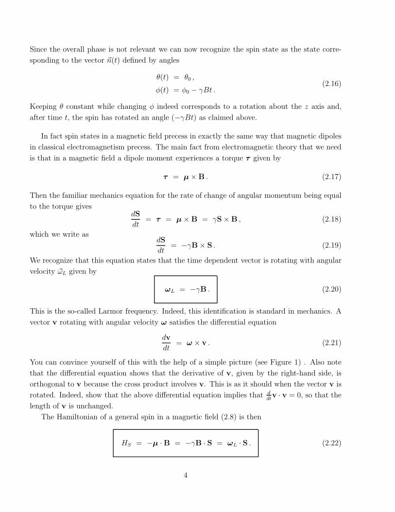
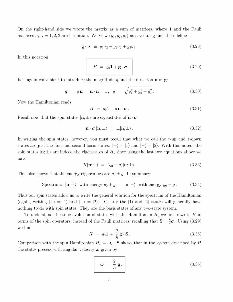
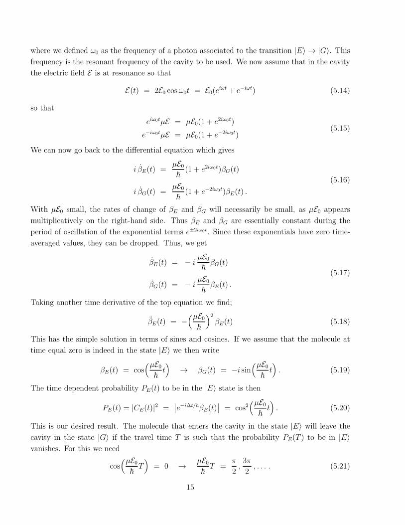

MIT OpenCourseWare httpocwmitedu
805 Quantum Physics II Fall 2013
For information about citing these materials or our Terms of Use visit httpocwmiteduterms


![Quantum Physics [Berkeley Physics Course Wichmann]](https://static.fdocuments.in/doc/165x107/55cf9bfa550346d033a815f4/quantum-physics-berkeley-physics-course-wichmann.jpg)


