Quantum Monte Carlo Studies of the Structure of Light Nuclei · Quantum Monte Carlo Studies of the...

Quantum Monte Carlo Studies ofthe Structure of Light Nuclei

Robert B. Wiringa

Physics Division, Argonne National Laboratory

WORK WITH

Joe Carlson, Los Alamos

Ken Nollett, Argonne

Muslema Pervin, Argonne

Steve Pieper, Argonne

Rocco Schiavilla, Jefferson Lab & Old Dominion

Work not possible without extensive computer resources:

Argonne Laboratory Computing Resource Center (Jazz)Argonne Math. & Comp. Science Division (BlueGene/L)

NERSC IBM SP’s (Seaborg, Bassi)

Work supported by U.S. Department

of Energy, Office of Nuclear PhysicsPhysics Division

GOAL OF ab-initio L IGHT-NUCLEI CALCULATIONS

We seek to understand nuclei as collections of interacting nucleons by reliably solving the

many-nucleon Schrodinger equation for realistic Hamiltonians of the form

H =X

i

Ki +X

i<j

vij +X

i<j<k

Vijk + ...

Using quantum Monte Carlo methods we want to compute

• Binding energies, excitation spectra, relative stability

• Densities, moments, transition amplitudes, cluster-cluster overlaps

• Low-energyNA & AA scattering, astrophysical reactions

With accurate calculations we can rigorously test a given Hamiltonian.

At present our methods are limited to light (A ≤ 12) nuclei

and local potentials with weak quadratic-momentum dependence.

ARGONNE V18

Ki = − ~2

4[( 1

mp+ 1

mn) + ( 1

mp− 1

mn)τzi]∇

2i

vij = vγij + vπ

ij + vIij + vS

ij =P

p vp(rij)Opij

vγij : pp, pn & nn electromagnetic terms

vπij ∼ [Yπ(rij)σi · σj + Tπ(rij)Sij ] ⊗ τ i · τj

vIij =

P

p IpT 2

π (rij)Opij

vSij =

P

p[P p +Qpr + Rpr2]W (r)Opij

Opij = [1, σi · σj , Sij ,L · S,L2,L2(σi · σj), (L · S)2]

+ [1, σi · σj , Sij ,L · S,L2,L2(σi · σj), (L · S)2] ⊗ τi · τj

+ [1, σi · σj , Sij ,L · S] ⊗ Tij

+ [1, σi · σj , Sij ,L · S] ⊗ (τiz + τjz)

Sij = 3σi · rijσj · rij − σi · σj Tij = 3τizτjz − τi · τj

Fits Nijmegen PWA93 data base of 1787pp & 2514np observables forElab ≤ 350 MeV

with χ2/datum = 1.1 plusnn scattering length and2H binding energy

0 0.5 1 1.5 2r (fm)

-150

-100

-50

0

50

100

150

200

250V

(M

eV)

vc

vτvσvστv

tv

tτ

Argonne v18

THREE-NUCLEON POTENTIALS

Urbana IX (UIX)

Vijk = V 2πPijk + V R

ijk

Illinois 2 (IL2)

Vijk = V 2πPijk + V 2πS

ijk + V 3π∆Rijk + V R

ijk

THE MANY-BODY PROBLEM

Need to solve

HΨ(~r1, ~r2, · · · , ~rA; s1, s2, · · · , sA; t1, t2, · · · , tA) = EΨ(~r1, ~r2, · · · , ~rA; s1, s2, · · · , sA; t1, t2, · · · ,

si are nucleon spins:± 12

ti are nucleon isospins (proton or neutron):± 12

2A ×“

AZ

”

complex coupled2nd order differential equations in3A dimensions

(number of isospin states can be reduced)

12C: 270,336 coupled equations in 36 dimensions

Coupling is strong:

• 〈vtensor〉 is ∼ 60% of total 〈vij〉

• 〈vtensor〉 = 0 if no tensor correlations

-1 0 1

-1

0

1

fem

tom

eter

MJ = 0

femtometer-1 0 1

-1

0

1

MJ = 1

VARIATIONAL MONTE CARLO

Minimize expectation value ofH

EV =〈ΨV |H|ΨV 〉

〈ΨV |ΨV 〉≥ E0

Trial function (s-shell nuclei)

|ΨV 〉 =

2

41 +X

i<j<k

UT NIijk

3

5

"

SY

i<j

(1 + Uij)

# "

Y

i<j

fc(rij)

#

|ΦA(JMTT3)〉

|Φd(1100)〉 = A| ↑ p ↑ n〉 ; |Φα(0000)〉 = A| ↑ p ↓ p ↑ n ↓ n〉

Uij =X

p=2,6

up(rij)Opij ; UT NI

ijk = −ǫVijk(rij , rjk, rki)

Functionsfc(rij) andup(rij) are obtained numerically from solution of coupled differential

equations containingvij .

Correlation functions

0 1 2 3 4 5 6 7 8r (fm)

−0.6

−0.4

−0.2

0.0

0.2

0.4

0.6

0.8

1.0

1.2

fc,utτ (2H)

fc,utτ (3H)

fc,utτ (4He)

fsp,utτ (6Li)

φp (6Li)

fc

10 utτ

φp

fsp

[f c(4He)]

3

[f c(3H)]

2

Trial function (p-shell nuclei)

⇒ A

8

<

:

Y

i<j≤4

fss(rij)X

LS[n]

“

βLS[n]

Y

k≤4<l≤A

fsp(rkl)Y

4<l<m≤A

fpp(rlm)

|Φα(0000)1234Y

4<l≤A

φLS[n]p (Rαl)

˘

[Yml1 (Ωαl)]LML

⊗ [χl(12ms)]SMS

¯

JM[νl(

12t3)]T T3

〉

9

=

;

Permutation symmetry

A [n] L (T, S)

6 [2] 0, 2 (1, 0), (0, 1)

[11] 1 (1, 1), (0, 0)

7 [3] 1, 3 (1/2, 1/2)

[21] 1, 2 (3/2, 1/2), (1/2, 3/2), (1/2, 1/2)

[111] 0 (3/2, 3/2), (1/2, 1/2)

8 [4] 0, 2, 4 (0, 0)

[31] 1, 2, 3 (1, 1), (1, 0), (0, 1)

[22] 0, 2 (2, 0), (1, 1), (0, 2), (0, 0)

[211] 1 (2, 1), (1, 2), (1, 1), (1, 0), (0, 1)

Diagonalization

in βLS[n] basis to produce energy spectraE(Jπx ) and orthogonal excited statesΨV (Jπ

x )

Expectation values

ΨV (R) represented by vector with2A × (AZ) spin-isospin components for each space

configurationR = (r1, r2, ..., rA); Expectation values are given by summation over samples

drawn from probability distributionW (R) = |ΨP (R)|2:

〈ΨV |O|ΨV 〉

〈ΨV |ΨV 〉=

X Ψ†V (R)OΨV (R)

W (R)/

X Ψ†V (R)ΨV (R)

W (R)

Ψ†Ψ is a dot product andΨ†OΨ a sparse matrix operation.

Scaling of calculation

A P NS × NTQ

(×8Be)

4He 4 6 16×2 0.001

6Li 6 15 64×5 0.036

8Be 8 28 256×14 1.10B 10 45 1024×42 24.12C 12 66 4096×132 530.

GREEN’ S FUNCTION MONTE CARLO

Projects out lowest energy state from variational trial function

Ψ(τ) = exp[−(H − E0)τ ]ΨV =X

n

exp[−(En − E0)τ ]anψn

Ψ(τ → ∞) = a0ψ0

Evaluation ofΨ(τ) done stochastically in small time steps∆τ

Ψ(Rn, τ) =

Z

G(Rn,Rn−1) · · ·G(R1,R0)ΨV (R0)dRn−1 · · · dR0

using the short-time propagator accurate to order(∆τ)3

Gαβ(R,R′) = eE0δτG0(R,R′)〈α|

"

SY

i<j

gij(rij , r′ij)

g0,ij(rij , r′ij)

#

|β〉

where the free many-body propagator is

G0(R,R′) = 〈R|e−Kτ |R′〉 =

»r

m

2π~2τ

–3A

exp

»

−(R − R′)2

2~2τ/m

–

andg0,ij andgij are the free and exact two-body propagators

gij(rij , r′ij) = 〈rij |e

−Hijτ |r′ij〉

Mixed estimates

〈O(τ)〉Mixed =〈ΨV |O|Ψ(τ)〉

〈ΨV |Ψ(τ)〉; 〈O(τ)〉 ≈ 〈O(τ)〉Mixed + [〈O(τ)〉Mixed − 〈O〉V ]

〈H(τ)〉Mixed =〈Ψ(τ/2)|H|Ψ(τ/2)〉

〈Ψ(τ/2)|Ψ(τ/2)〉≥ E0

Propagator cannot containp2, L2, or (L · S)2 operators:

Gβα(R′,R) has onlyv′8〈v18 − v′8〉 computed perturbatively with extrapolation (small for AV18)

Reliable in Faddeev (3H), hyperspherical harmonic & Yakubovsky (4He) comparisons

Fermion sign problem limits maximumτ :

Gβα(R′,R) brings in lower-energy boson solution

〈ΨT |H|Ψ(τ)〉 projects back fermion solution

Exponentially growing statistical errors

Constrained-path propagation, removes steps that have

Ψ†(τ,R)Ψ(R) = 0

Possible systematic errors reduced by10−20 unconstrained steps before evaluating observables.

GFMC propagation of three states in6Li

0 0.5 1 1.5 2 2.5

-32

-30

-28

-26

-24

τ (MeV-1)

E(τ

) (

MeV

)

2+

3+

gs

6Li

α+d

GFMC FOR SECOND EXCITED STATES OF SAMEJπ

TheΨT are constructed by non-orthogonal basis diagonalization in p-shell wave functions.

Example:7Li(5/2-) has 4 symmetry possibilities:2F[43] , 4P[421] ,4D[421] , 2D[421]

〈ΨT (2nd 52

−)|ΨT (1st 5

2

−)〉 = 0 , but〈ΨGFMC(2

nd 52

−)|ΨT (1st 5

2

−)〉 need not be zero.

Will e−(H−E0)τΨT (2nd 52

−) → ΨGFMC(1

st 52

−) ?

Can use〈ΨGFMC(i)|H|ΨGFMC(j)〉 and〈ΨGFMC(i)|ΨGFMC(j)〉 to rediagonalize

0 0.2 0.4 0.6 0.8 1-35

-30

-25

-20

-15

τ (MeV-1)

E(τ

) (

MeV

)

4th 5/2-

3rd 5/2-

2nd 5/2-

1st 5/2-

7Li(5/2-)AV18 + Illinois-2

GFMC Propagation

0 0.2 0.4 0.6 0.8 1

-0.05

-0.03

-0.01

0.01

0.03

τ (MeV-1)

⟨Ψi|Ψ

1⟩

⟨Ψ2|Ψ1⟩⟨Ψ3|Ψ1⟩⟨Ψ4|Ψ1⟩

Binding energy results forA=3,4

Hamiltonian Method 3H 3He 4He

Argonnev′

8VMC* 25.44(2)

(no EM) GFMC1 25.93(2)

FY2 25.94(5)

HH3 25.90(1)

SVM4 25.92

EIHH5 25.944(10)

CRCGV6 25.90

NCSM7 25.80(20)

Argonnev18 VMC* 7.50(1) 6.77(1) 23.70(2)

GFMC1 7.61(1) 6.89(1) 24.07(4)

F/FY2 7.623 6.924 24.28

PHH/HH3 7.623 6.925 24.18

Argonnev18 VMC* 8.31(1) 7.56(1) 27.72(2)

+ Urbana IX GFMC1 8.46(1) 7.70(1) 28.33(2)

F/FY2 8.478 7.760 28.50

PHH/CHH3 8.480 7.749 28.46

Experiment 8.482 7.718 28.296

* Arriaga, Pandharipande, Wiringa 1 Carlson, Pieper, Wiringa 2 Kamada, Nogga, Glockle 3 Viviani, Kievsky, Rosati

4 Varga, Suzuki 5 Barnea, Leideman, Orlandini 6 Hiyama, Kamimura 7 Navratil, Barrett

-70

-65

-60

-55

-50

-45

-40

-35

-30

-25

-20

Ene

rgy

(MeV

)

α+d

α+t

2α 2α+n9Be+n

6Li+α

ΨT

GFMC

0+

4He 1+

3+2+

6Li3/2−1/2−

7/2−5/2−

7Li

0+

2+

4+

1+3+

8Be3/2−

5/2−1/2−7/2−9/2−

9Be0+2+

3+

4+

1+

10Be3+1+2+

4+

10B

α+d

α+t

2α 2α+n9Be+n

6Li+αArgonne v18 + IL2

VMC Trial &GFMC Calculations

-60

-55

-50

-45

-40

-35

-30

-25

-20E

nerg

y (M

eV)

α+2n

α+d

α+t

6He+2n

7Li+n

2α

AV18

UIXIL2 Exp

0+

4He

1+

0+

2+

6He 1+

3+2+1+

6Li

5/2−

5/2−

3/2−1/2−

7/2−5/2−5/2−

7/2−

3/2−

7Li

1+

0+

2+

8He

2+1+

0+

3+1+

4+

8Li

0+

2+

4+

2+1+3+

8Be

α+2n

α+d

α+t

6He+2n

7Li+n

2α

Argonne v18without & with various Vijk

GFMC Calculations

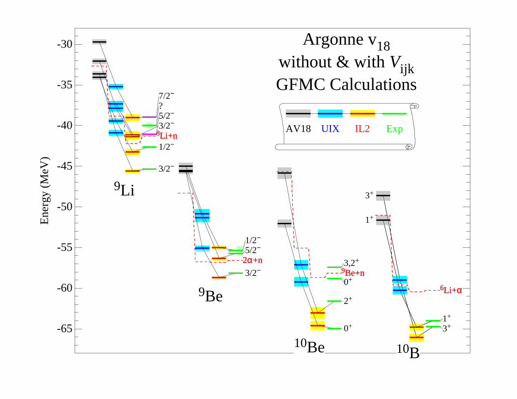
-65

-60

-55

-50

-45

-40

-35

-30E

nerg

y (M

eV)

8Li+n

2α+n9Be+n

6Li+α

AV18 UIX IL2 Exp3/2−

3/2−

1/2−

?5/2−

7/2−

9Li

3/2−

5/2−1/2−

9Be

0+

2+

0+

3,2+

10Be3+1+

10B

3+

1+

8Li+n

2α+n9Be+n

6Li+α

Argonne v18without & with VijkGFMC Calculations

-100

-90

-80

-70

-60

-50

-40

-30

-20

-10

0E

nerg

y (M

eV)

AV18

IL2 Exp

1+

2H 1/2+

3H

0+

4He 1+3+2+

6Li 3/2−1/2−7/2−5/2−

7Li 2+1+

0+

3+

4+

8Li0+2+

4+

1+3+

8Be

3/2−1/2−5/2−7/2−

9Li

9/2−

5/2+

7/2+

3/2+

1/2+

3/2−5/2−1/2−

7/2−

9Be

3+1+

0+2+

4+

0+2+,3+

10Be3+1+2+4+

10B

3+

1+

2+4+

0+

12C

Argonne v18With Illinois-2

GFMC Calculations

-5

0

5

10

15

20

25E

xcita

tion

ener

gy (

MeV

)

AV18 +IL2 Exp

1+

0+

2+

2+0+

6He

1+

1+

3+

2+

1+

6Li

5/2−

5/2−

3/2−1/2−

7/2−

5/2−5/2−

7/2−

3/2−1/2−

7Li

2+

2+

2+1+

0+

3+1+

4+

3+

1+

8Li

1+

0+

2+

4+

2+1+3+

4+

0+

2+

3+2+

8Be

3/2−

3/2−

1/2−

?

5/2−

7/2−

9Li

9/2−3/2−

5/2+

7/2+

3/2+

1/2+

3/2+

3/2−1/2+5/2−1/2−5/2+3/2+

7/2−

3/2−

5/2−

9/2+

5/2+7/2+

9Be

0+

3+

2+

1+

0+

2+1−

2−

2+

4+

0+

2+,3+

10Be

3+1+

2+

2−

4+

1+

3+

1+2+

3+

10B

3+

1+

2+

2−

4+

1+

3+

1+

2+

Argonne v18With Illinois-2

GFMC Calculations 4 March 2006

NEW ILLINOIS POTENTIALS – PROGRESSREPORTI

• Illinois 1–5 parameters determined in 2000.

– Fits made toA ≤ 8 only

– Preliminary nuclear matter calculations at Urbana (Morales, Pandharipande, Ravenhall)

suggested at most IL2 is viable

– Improved GFMC results in worse8He agreement

• Started new fitting up toA = 10

• Michele Viviani (Pisa) finds sign error in one piece ofAσ in V 3πijk

– Formula was published correctly, but incorrectly programmed

– Increased attraction for all nuclei

• New fit made with correctedAσ : IL7

– parameters weaker than for IL2 because of increased attraction

– better quality reproduction of energies than IL2

– so far have not found any significant difference in other observables

• Nuclear and neutron matter are probably still too soft

-70

-65

-60

-55

-50

-45

-40

-35

-30

-25

-20E

nerg

y (M

eV)

IL2IL7

Exp

0+

4He

1+

0+2+

2+0+

6He

1+

1+

3+

2+1+

6Li

3/2−

3/2−

1/2+

5/2+

1/2−

3/2−

5/2−

(5/2)−

7He

5/2−5/2−

3/2−1/2−

7/2−5/2−5/2−

7/2−

3/2−1/2−

7Li

1+0+2+

0+

2+

8He 2+

2+

2+1+

0+

3+1+

4+

3+

1+

8Li

1+

0+

2+

4+

2+1+

3+4+

0+

2+

3+2+

8Be

1/2−

9He

3/2−

3/2−1/2−

?5/2−

7/2−

9Li

9/2−3/2−

5/2+

7/2+

3/2+

1/2+

3/2+

3/2−1/2+5/2−1/2−5/2+3/2+

7/2−

3/2−

5/2−

9/2+

5/2+7/2+

9Be

0+

10He

2+

0+

(1-,2-)1+

10Li0+

3+

2+

1+

0+2+1−

2−

2+

4+

0+

3,2+

10Be 3+1+

2+

2−

4+

1+

3+

1+2+

3+

10B

Argonne v18With Illinois Vijk

GFMC Calculations22 October 2007

GFMC FOR SCATTERING STATES

GFMC treats nuclei as particle-stable system – should be good for energies of narrow resonances

Need better treatment for locations and widths of wide states and for capture reactions

METHOD

• Pick a logarithmic derivative,χ, at some large boundary radius (RB ≈ 9 fm)• GFMC propagation, using method of images to preserveχ atR, findsE(RB, χ)

• Phase shift,δ(E), is function ofRB , χ,E• Repeat for a number ofχ until δ(E) is mapped out

Example for5He(12

−)

• “Bound-state” boundarycondition does notgive stable energy;Decaying to n+4Hethreshold

• Scattering boundarycondition producesstable energy.

0 0.1 0.2 0.3 0.4-27

-26

-25

-24

-23

τ (MeV-1)

E(τ

) (

MeV

)

"bound state"

Log-deriv = -0.168 fm-1

4He + n – PARTIAL-WAVE CROSS SECTIONS

• Hale phase shifts fromR-matrix

analysis up toJ = 92

of data

• Tilted error bars from

δ(RB , χ, E ± ∆E)

• AV18+IL2 was not fit to5He,

good prediction of32

−& 1

2

−

resonances (both locations

and widths)

• 4He+n scattering length also

well reproduced

Nollett, et al., Phys.Rev.Lett.99, 022502 (2007)

0 1 2 3 4 50

1

2

3

4

5

6

7

Ec.m. (MeV)

σ LJ

(b)

12

+

12

-

32

-

R-Matrix

Pole location

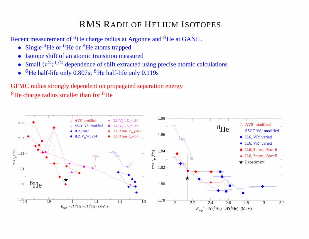
RMS RADII OF HELIUM ISOTOPES

Recent measurement of6He charge radius at Argonne and8He at GANIL• Single4He or6He or8He atoms trapped• Isotope shift of an atomic transition measured• Small〈r2〉1/2 dependence of shift extracted using precise atomic calculations• 6He half-life only 0.807s;8He half-life only 0.119s

GFMC radius strongly dependent on propagated separation energy8He charge radius smaller than for6He

0.8 0.9 1 1.1 1.2 1.31.86

1.90

1.94

1.98

2.02

2.06

Esep′ = H′(4He) - H′(6He) (MeV)

rms

r p (f

m)

AV8’ modified

SSCC V8’ modified

IL2, other

IL2, VR’=1.254

IL6, VR’, ES=1.84

IL6, VR’, ES=1.48

IL6, 3 trm, RWS=4.0

IL6, 3 trm, ES=1.4

6He

2 2.2 2.4 2.6 2.8 3 3.21.78

1.80

1.82

1.84

1.86

1.88

Esep′ = H′(6He) - H′(8He) (MeV)

rms

r p (f

m)

AV8’ modified

SSCC V8’ modified

IL6, VR’ varied

IL6, VR’ varied

IL6, 3=trm, l3bc=6

IL6, 3=trm, l3bc=5

Experiment

8He

4,6,8HE DENSITIES

• 4He central density twice that of nuclear matter!• Neutrons drag4He center of mass around – spread out density

– results in charge radius of6He> 4He (2.08 fm vs 1.66 fm)• 6He & 8He have large neutron halos due to weak binding of neutrons• Neutron halo of6He more diffuse than that of8He – smallerEsep

0 0.5 1 1.5 2 2.5 30.00

0.05

0.10

0.15

r (fm)

Den

sity

(fm

-3)

4He6He - Proton6He - Neutron8He - Proton8He - Neutron

0 2 4 6 8 10 1210-5

10-4

10-3

10-2

10-1

r (fm)

Den

sity

× r2

(f

m-1

)

4He6He - Proton6He - Neutron8He - Proton8He - Neutron

TWO-NUCLEON DENSITIES

ρpp(r) =X

i<j

〈Ψ|δ(r − |ri − rj |)1 + τi

2

1 + τj

2|Ψ〉

0 0.5 1 1.5 2 2.5 30.000

0.005

0.010

0.015

0.020

r12 (fm)

ρ pp

(fm

-3)

4He6He - Proton8He - Proton

pair rms radii

rpp rnp rnn4He 2.41 2.35 2.416He 2.51 3.69 4.408He 2.52 3.58 4.37

TWO-NUCLEON KNOCKOUT – (e, e′pN)

• Recent (still being analyzed) JLab expt. for12C(e, e′pN)

• Measured back to backpp andnp pairs• Pairs with relative momentum 2–3 fm−1 show 10–20× np enhancement (preliminary).

0 1 2 3 4 5q (fm

-1)

10-1

100

101

102

103

104

105

ρ NN(q

,Q=

0) (

fm6 )

AV18/UIX 4He

AV4’4He

pp np

0 1 2 3 4 5q (fm

-1)

10-1

100

101

102

103

104

105

106

ρ NN(q

,Q=

0) (

fm6 )

3He

4He

6Li

8Be

• VMC calculations for3He,4He, and8Be show this effect

• Effect disappears when tensor correlations are turned off

• Shows importance of tensor correlations to> 2 fm−1.

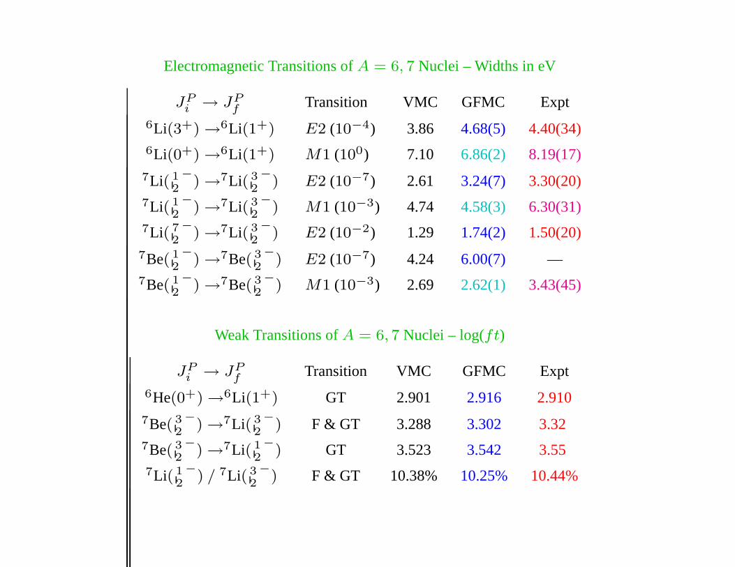
Electromagnetic Transitions ofA = 6, 7 Nuclei – Widths in eV

JPi → JP

f Transition VMC GFMC Expt6Li(3+) →6Li(1+) E2 (10−4) 3.86 4.68(5) 4.40(34)6Li(0+) →6Li(1+) M1 (100) 7.10 6.86(2) 8.19(17)7Li( 1

2

−) →7Li( 3

2

−) E2 (10−7) 2.61 3.24(7) 3.30(20)

7Li( 12

−) →7Li( 3

2

−) M1 (10−3) 4.74 4.58(3) 6.30(31)

7Li( 72

−) →7Li( 3

2

−) E2 (10−2) 1.29 1.74(2) 1.50(20)

7Be( 12

−) →7Be( 3

2

−) E2 (10−7) 4.24 6.00(7) —

7Be( 12

−) →7Be( 3

2

−) M1 (10−3) 2.69 2.62(1) 3.43(45)

Weak Transitions ofA = 6, 7 Nuclei – log(ft)

JPi → JP

f Transition VMC GFMC Expt6He(0+) →6Li(1+) GT 2.901 2.916 2.9107Be( 3

2

−) →7Li( 3

2

−) F & GT 3.288 3.302 3.32

7Be( 32

−) →7Li( 1

2

−) GT 3.523 3.542 3.55

7Li( 12

−) / 7Li( 3

2

−) F & GT 10.38% 10.25% 10.44%

Isospin-mixing in8Be

Experimental energies of 2+ states

Ea = 16.626(3) MeV

Eb = 16.922(3) MeV

and 2α decay widths:

Γa = 108.1(5) keV

Γb = 74.0(4) keV

Assume isospin mixing of 2+;1 and 2+;0*

states due to isovector interactionH01:

Ψa = αΨ0 + βΨ1

Ψb = βΨ0 − αΨ1

α2 + β2 = 1

Decay throughT = 0 component only

Γa/Γb = α2/β2

α = 0.7705(15)

β = 0.6375(19)

-60

-56

-52

-48

-44

-40

-36

Ene

rgy

(MeV

)

8Li

2+;1

3P[431]

7Li+n

1+;1

3+;13

D[431]

8Be

α+α0

+;01

S[44]

2+;01

D[44]

4+;01

G[44]

2+;0+1

1+;1

1+;0

3+;0+1

8B

2+;1

7Be+p

1+;1

3P[431]

Ea,b =H00 + H11

2±

s

„

H00 − H11

2

«2

+ (H01)2

H00 = 16.746(2) MeV

H11 = 16.802(2) MeV

H01 = −145(3) keV

F. C. Barker [Nucl.Phys.83, 418 (1966)] estimated the Coulomb matrix element

connecting the 2+;1 and 2+;0* states asHC01 = −67 keV

The 1+;1 and 1+;0 and the 3+;1 and 3+;0 levels also mix, but decay by nucleon emission. Barker assigns

values of:

α1 = 0.24 ; β1 = 0.97 ; H01 = −120(1) keV

α3 = 0.41 ; β3 = 0.91 ; H01 = −62(15) keV

Isospin-mixing matrix elements in keV

H01 KCSB V CSB Vγ (Coul) (Mag)

2+;1⇔2+;0* VMC −107(2) −2.5(2) −23.8(4) −80.8(12) −69.4(11) −11.4(1)

GFMC −115(3) −3.1(2) −21.3(6) −90.3(26) −78.3(25) −12.0(2)

Barker −145(3) −67

1+;1⇔1+;0 VMC −70(1) −1.8(1) −17.5(3) −50.4(9) −50.6(9) 0.2(1)

GFMC −102(4) −2.9(2) −18.2(6) −80.3(30) −79.5(30) −0.8(2)

Barker −120(1) −54

3+;1⇔3+;0 VMC −67(1) −1.4(1) −12.7(3) −52.0(6) −41.0(6) −12.0(2)

GFMC −90(3) −2.5(2) −14.8(6) −73.1(21) −60.9(21) −12.2(2)

Barker −62(15) −32

2+;1⇔2+;0 VMC −13(1) −0.2(1) −2.4(1) −10.4(3) −6.1(2) −4.3(1)

GFMC −6(2) −0.4(2) −1.3(4) −4.4(12)

CONCLUSIONS

We have made much progress in calculating light nuclei

• 1 − 2% calculations ofA = 6 – 12 nuclear energies are possible• Illinois Vijk give average binding-energy errors< 0.7 MeV for A = 3 − 12

– Vijk required for overallP -shell energies

– Also required for spin-orbit splittings and several levelorderings• Charge radii are in good agreement with experiment• GFMC for off-diagonal matrix elements in progress• GFMC for scattering states has been initiated• VMC calculations of single- and multi-nucleon momentum distributions

and there is still much to do

• Lots of scattering states and reactions to be done– n+3H, p+α, n+6He, n+8He, n+9Li, α+α, etc.– astrophysical reactions:3He+α →7Be, p+7Be→8B, n+(α+α) →9Be, etc.

– All big-bang nucleosynthesis, solar, & somer-process seeding reactions should be accessible

• Calculations of– overlaps, spectroscopic factors, asymptotic normalization coefficients– electromagnetic and weak transitions inA ≥ 8 nuclei– meson-exchange current contributions to moments and transitions– more unnatural-parity &2~ω excited states

• 12C including 2nd 0+ (Hoyle) state

Quantum Monte Carlo Studies of the Structure of Light Nuclei · Quantum Monte Carlo Studies of the...

Documents

Transcript of Quantum Monte Carlo Studies of the Structure of Light Nuclei · Quantum Monte Carlo Studies of the...