Quantum Monte Carlo fornanosystems and materials:

Electronic structure andDynamics

Jeffrey C. GrossmanCOINS, UC Berkeley

Lubos MitasNorth Carolina State University

San Sebastian, July 2007

Motivation: QMC for nanosystems and materials

• nanosystems are challenging: larger than molecules but noperiodicity of solids, outside of traditional paradigms

• often unknown both atomic and electronic structures: discoveriesof “new chemistry” and phenomena with large impact of electroncorrelation due to the variety of boundary conditions (free, …)

• small changes in geometry or adding/subtracting an electron:dramatic effect on both electronic and atomic structures

• nanosystems often of sizes out of the reach of basis set correlated wavefunction electronic structure methods

• QMC reaches beyond DFT: optical gaps, accurate bindingenergies, reaction barriers …

Fixed-node QMC in a nutshell

In DMC walkers evolve in 3Ne -dimensions and sample thewavefunction according to thetime-dependent Schrodingerequation in propagation time

φ( r,t) = exp(-tH)φ( r,t=0)

f(r,t) = φ( r,t) φTRIAL( r) > 0,fixed-node condition

diffusion, drift, reweighting

φTRIAL( r) = det[φ _a] det[φ_b]exp(U_corr)

The simplest trial wave function:

The first application of QMC to nanosystems: What is the lowest energy isomer of C_20 ???

ring bowl cage

J.C. Grossman, L. Mitas, K. Raghavachari, Phys. Rev. Lett. 75, 3870 (1995)

QMC was the first method to predict the correct ordering (late confirmed by others)

J.C. Grossman, L. Mitas, K. Raghavachari, Phys. Rev. Lett. 75, 3870 (1995)

Another example: evaluate correlation energy froma single atom to molecules, clusters, all the way upto the solid!

J.C. Grossman, L. Mitas, Phys. Rev. Lett. 74, 1323 (1995)

Transition metal and oxygen: tests on molecules(L.K. Wagner, ‘03)

DMC with HF orbitals ExperimentTiO 6.4(1) eV 6.87(7) eVMnO 2.7(1) eV 3.70 eV

Errors up to 1 eV!

Multi-determinant (MCSCF) wavefunction ~ 20 determinants:TiO 6.7(1) eVMnO 3.4(2) eV

MCSCF not bad, but expensive and not practical for solids.Look at the wavefunction/orbitals ...

Look at the orbitals: Hartree-Fock vs B3LYP,the charge transfer vs. more covalent bonding

Hartree-FockB3LYP

O Mn MnO

Optimization of the weight of exact exchange tominimize the fixed-node error

MnO molecule binding by various methods

FN DMC with B3LYP orbitals within 0.2 eV of experiment

Magnetic "nanodots": caged transition elementsTM@Si12 TM=Sc, Ti, ... 3d, 4d, 5d (P. Sen, ‘03) APS March Meeting in '94:L. M.: Electronic structure of Mn@Si12

- attempt to predict caged d-spin - no success, hybridized, unstable

Experiment in Japan in '01! W@Si12

Other transition metal atoms ?

Difference high-spin vs low-spin state:prediction of Si12Ti as a high-spin system

Ehigh-spin - Elow-spin

Example of a large-scale challenging calculation:FeO solid, B1 -> B8 phase transition (J. Kolorenc,NCSU, ‘07)

- FeO ground state: B1 structure, antiferromagnetic insulator- DFT: wrong structure (B8) and wrong electronic state (metal)

QMC: - Ne-core relativistic pseudopotentials for Fe - 16 FeO supercell, 352 valence e- - fixed-node DMC

Cohesive energy[eV]: LDA HF B3LYP DMC Exper. 11.7 5.9 7.9 9.47(4) ~9.7

Gap [eV]: LDA HF B3LYP DMC Exper. 0 10.2 3.4 2.8(4) ~ 2.2

DMC transition B1->B8 pressure 70(5) GPa, Exper. ~70-100GPa !

Summary of the fixed-node DMC (“plain vanilla”)method

- fixed-node DMC typically recovers about 95% of the valence correlation energy (done for up to ~ 1000 electrons)

- energy differences agree with experiments within a few %

- method scales like a N^2-3 where N is the number of valence electrons (core electrons eliminated by pseudopotentials)

- applied to a number of systems, eg, electron gas and quantum liquids, atoms, molecules, solids etc; often the results became benchmarks for other methods - about two orders of magnitude slower than mean-field methods but very efficient (perfectly scalable) on parallel architectures

Computational aspects of the fixed-node DMC

- sampling walkers (almost) independent -> flexibility current developments: scale up to 100,000 compute cores!!!

- cycle intensive, less memory intensive

- can accommodate any basis, any type of trial function

- enable to focus on interesting physics: types of many-body effects which are important, symmetries, phases, processes - correlation problem “cornered” into the last 5% of E_corr!

Beyond static calculations: couple QMC with ab initio molecular dynamics for studies of dynamical effects and T>0

• ab initio molecular dynamics (AIMD) based on density functionaltheory (DFT) is an exceptionally powerful simulation tool:dynamics, T>0, …

• however,certain properties need accuracy beyond DFT: opticalgaps, accurate binding energies, reaction barriers …

• how to improve the accuracy over DFT ?

Employ quantum Monte Carlo ! (or GW-BSE, possibly others)

Easy to say …

Total Energy vs Time

QMC energies in an AIMD simulation: expensive!

• Current approach was to take snapshots of the AIMD trajectory anddo a full fixed-node diffusion MC (DMC) run for each point.

• Example: hot silane molecule (T~1500K, 100 x1000 DMC steps!)

Optical Gap vs Time

Note: both MD and QMC propagate particles …

In DMC walkers evolve in 3Ne -dimensions and sample thewavefunction according to thetime-dependent Schrodingerequation in propagation time

In MD ions evolve accordingto the Newton’s law with abinitio ionic forces in real time

- gradI EDFT (R)= mI aI

φ( r,t) = exp(-tH)φ( r,t=0)

f(r,t) = φ( r,t) φTRIAL( r) > 0,fixed-node

diffusion, drift, reweighting

Coupling of QMC and MD: Basic Idea

Instead of discrete sampling of each point with a new QMC run:calculate QMC energies “on-the-fly” during the dynamic simulation !

Continuously update the DMC walkers so that they correctlyrepresent the evolving wavefunction

Evolution of both configuration spaces is coupled: as the ionicdynamical trajectories evolve, so does the population of DMCelectrons

average distance made byan ion in one MD time step

10-4 … 10-3 a.u.

average distance made by anelectron in a DMC time step

10-2 … 10-1 a.u.

Continuous DMC (CDMC) – naïve algorithm

• As the dynamical trajectory evolves, so does the population of DMCelectrons - the slow evolution in MD: highly welcome in DMC!

ab initio MD Step

R, Ψ(R)

DMC step

First Attempt (Simple)

Unstable walker population

Possible problems

• Wavefunction changes as ions move: bias in walker distribution ?• wrong wavefunction at the beginning of each step

• Dynamics of orbital occupations: orbital rotation, state crossings ?• swapping during dynamics

• Wavefunction changes as ions move: node crossing ?• electrons can cross nodes and nodes can cross electrons

Orbital swapping

It is possible that during the dynamics the ordering of states ischanged:

1

2,3,4

5

6

excitation

1

2,3,4

6

5

orb. swap

Solution:Before performing DMC step, calculate overlap of new orbitals withold. This is easy to estimate: the same set of walkers can be usedto perform the integral.

If overlap between same orbital is not 1 or between different orbitalsis not 0, then do a quick re-equilibration with VMC

It is easy to detect orbital swapping:

Most swaps are between occupied orbitals that were originally (at T=0K)degenerate states

For SiH4 one swap with unoccupied state over 2 ps simulation

Orbital overlaps

Node crossing

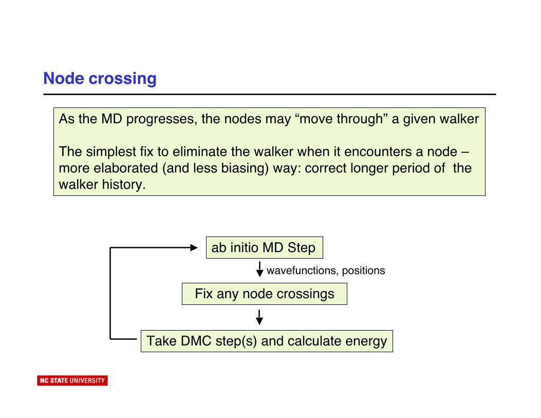
As the MD progresses, the nodes may “move through” a given walker

The simplest fix to eliminate the walker when it encounters a node –more elaborated (and less biasing) way: correct longer period of thewalker history.

ab initio MD Stepwavefunctions, positions

Fix any node crossings

Take DMC step(s) and calculate energy

Stable CDMC simulation

ab initio MD Step

Compute orb ital overlapswith current DMC walkers

Orbital swapping or rotation?

do VMCthen DMC

yes

noCheck for node crossings

compute weights

Take DMC step(s) and calculate energy

R, Ψ(R)

Successful CDMC Algorithm

•Stable DMC population

•How accurate is it?

•Benchmark against discrete DMC

•As simulation progresses, 1-stepCDMC energies begin to differsignificantly from discrete DMC

•Using 3 steps corrects time “lag”

•33 times more efficient thandiscrete sampling

CDMC: Number of DMC step needed per MD step

•Use large discrete sampled runs(1000 steps each) for comparison

E(discrete DMC) = -6.228(2)E(1 step continuous) = -6.220(2)E(2 steps continuous) = -6.220(2)E(3 steps continuous) = -6.226(2)E(10 steps continuous)= -6.230(2)E(20 steps continuous)= -6.228(2)

Thermal Averages (over 1 ps)

• Thermal averages are converged for N≥3

• Same convergence (3 CDMC steps)observed for Si2H6 and Si5H12

CDMC: Si2H6

As for SiH4, asymmetricallystretch molecule and let go

Average temperature ~ 1500 K

CDMC: Si2H6 Results

ForSi2H6, 3 stepsappears to lead tostability as for SiH4

# steps looks like afunction of dynamicsrather than size

Can pinpoint specifictypes of strain thatlead to wf lag

CDMC: H2O molecule dissociation path

• Test accuracy for dissociation problem: bond dissociation at ∆R~0.5 Å

• large-scale calculation: heat of vaporization for 32 water molecules: 6.1 kcal/mol, agrees with experiment -> dynamical, T>0 quantity

50 times moreefficient thandiscretesampling

J.C. Grossman, L. Mitas, Phys. Rev. Lett. 94, 056403 (2005)

CDMC: ionic trajectories in DFT, energies in QMC…

Emails from David Ceperley and Roberto Car:

Can you do it with QMC forces ?

• accurate energies (at the level of the fixed-node DMC)

• great for calculations of excited states andthermodynamic averages

• however, the ionic trajectories still generated from DFT …… (how disappointing) ?

Calculations of forces in QMC* vs DFT: SiH4

• DMC vs DFT forces: excellent agreement for Si,surprisingly close also for H

*Filipp i and Umrigar PRB (2000), Torelli and Mitas Theor. Prog. Phys. Supp. (2000), Casalegno,Mella, and Rappe JCP (2003), Assaraf and Caffarel JCP (2000), etc.

QMC/MD: no input from DFT (first time ever!)

QMC/MD total energy conservation for H_2

QMC/MD: dynamical proton dissociation from H2O

CDMC and QMC/MD: efficiency

For SiH4, to get a reasonable DMC energies over 2000 MD stepsusing discrete sampling, we need to take ~ 100,000 DMC steps

By comparison, CDMC requires 6,000 steps to accurately samplethe same trajectory

Cost of 3 CDMC steps for energy is less than cost of 1 MD step:CDMC introduces a small overhead to ab initio MD

Small MD step (and thus large correlation between atomicpositions) is huge advantage for CDMC because re-weighting isaccurate

Cost of accurate QMC forces in QMC/MD still significant: slowdownfactor of ~ 20 - 100

QMC as a modern and effective alternative forelectronic structure

- focus on efficient description many-body effects, put the many-body effects where they belongs: to the wavefunction (new wave function was/is always a milestone: Hartree-Fock, BCS, Laughlin...)

- input from other (CI,CC, etc) correlated wave function methods very important: efficiency!!! - one still has to do the physics/chemistry: which types of correlations, symmetries, phases, . . ., the fundamental and fun part!

- but: tedious integrals, averaging, etc, left to machines, gives a good use of parallelism, scales N^(1-3), robust, flexible

- often the most accurate method available: opens new insights into quantum many-body phenomena

QMC: only an accurate method or a paradigm shift ?

- in many cases it is more efficient to carry out the many-particle calculations than to (re)design a better mean-field - let the machine to worry about integrals etc ($/cycle decreasing exponentially in time)

- combination of analytical insights, reliable mean-fields and stochastic techniques a key for getting high accuracy solutions of Schr. eq.

- in working with wave functions one is closest to the many-body physics and understanding (fundamental point), the most efficient in capturing correlation effects - history of high accuracy benchmark/reference calculations and the only correlated wave function method which works also for solids

Conclusions

• QMC very successful in treatment of real nanosystems andmaterials: results often become accuracy benchmarks

• we have introduced a new efficient method for coupling abinitio molecular dynamics ionic with stochastic DMCelectronic steps to provide accurate DMC energies “on-the-fly”: CDMC

• accurate for both thermal averages and description ofenergies along the pathways

• we have carried out the first QMC/MD simulations usingboth forces and energies from QMC