![Statistical Mechanics Derived From Quantum Mechanics · More speci cally, the density matrix ^ˆ stin quantum statistical mechanics can be given by a general form [1] ˆ^ st(t) =](https://static.fdocuments.in/doc/165x107/5f33aa7686b2a20f55364b85/statistical-mechanics-derived-from-quantum-mechanics-more-speci-cally-the-density.jpg)
Quantum Mechanics: Density Functional Theory and Practical Application to Alloys
51
Quantum Mechanics: Density Functional Theory and Practical Application to Alloys Stewart Clark Condensed Matter Section Department of Physics University of Durham
description
Quantum Mechanics: Density Functional Theory and Practical Application to Alloys. Stewart Clark Condensed Matter Section Department of Physics University of Durham. Outline. Aim: To simulate real materials and experimental measurements - PowerPoint PPT Presentation
Transcript of Quantum Mechanics: Density Functional Theory and Practical Application to Alloys
Quantum Mechanics: Density Functional Theory and Practical
Application to AlloysStewart Clark
Condensed Matter SectionDepartment of PhysicsUniversity of Durham
Introduction to Computer Simulation: Edinburgh, May 2010
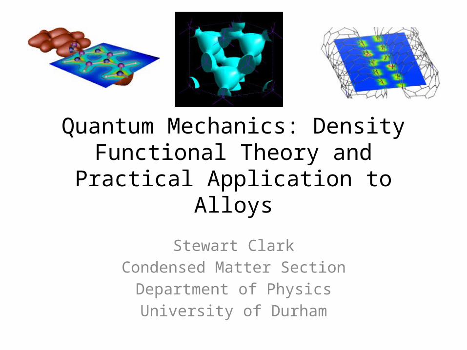
Outline
• Aim: To simulate real materials and experimental measurements
• Method: Density functional theory and high performance computing
• Results: Brief summary of capabilities and performing calculations
Introduction to Computer Simulation: Edinburgh, May 2010
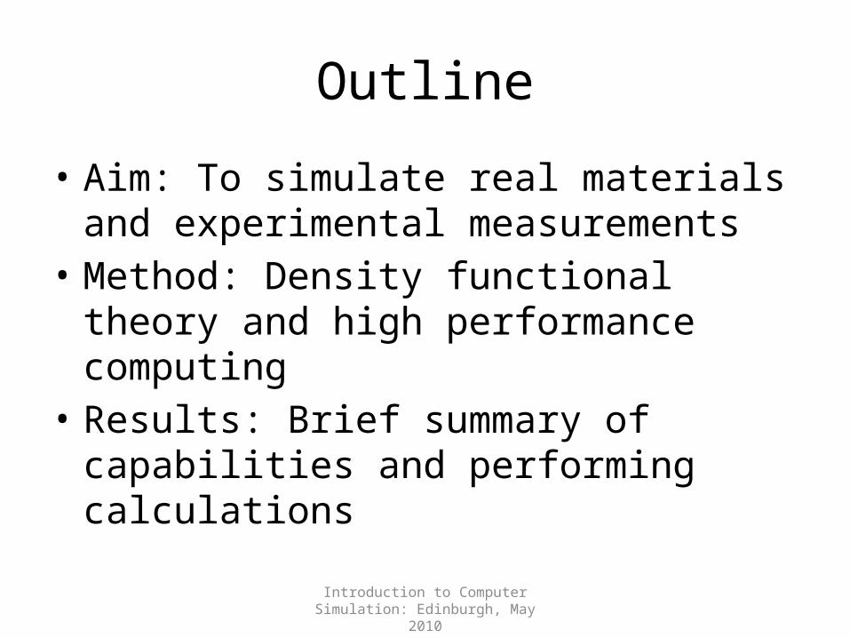
What would we like to achieve?
• Computers get cheaper and more powerful every year.
• Experiments tend to get more expensive each year.
• IF computer simulation offers acceptable accuracy then
at some point it should become cheaper than experiment.
• This has already occurred in many branches of science
and engineering.
• Possible to achieve this for properties of alloys?
Introduction to Computer Simulation: Edinburgh, May 2010
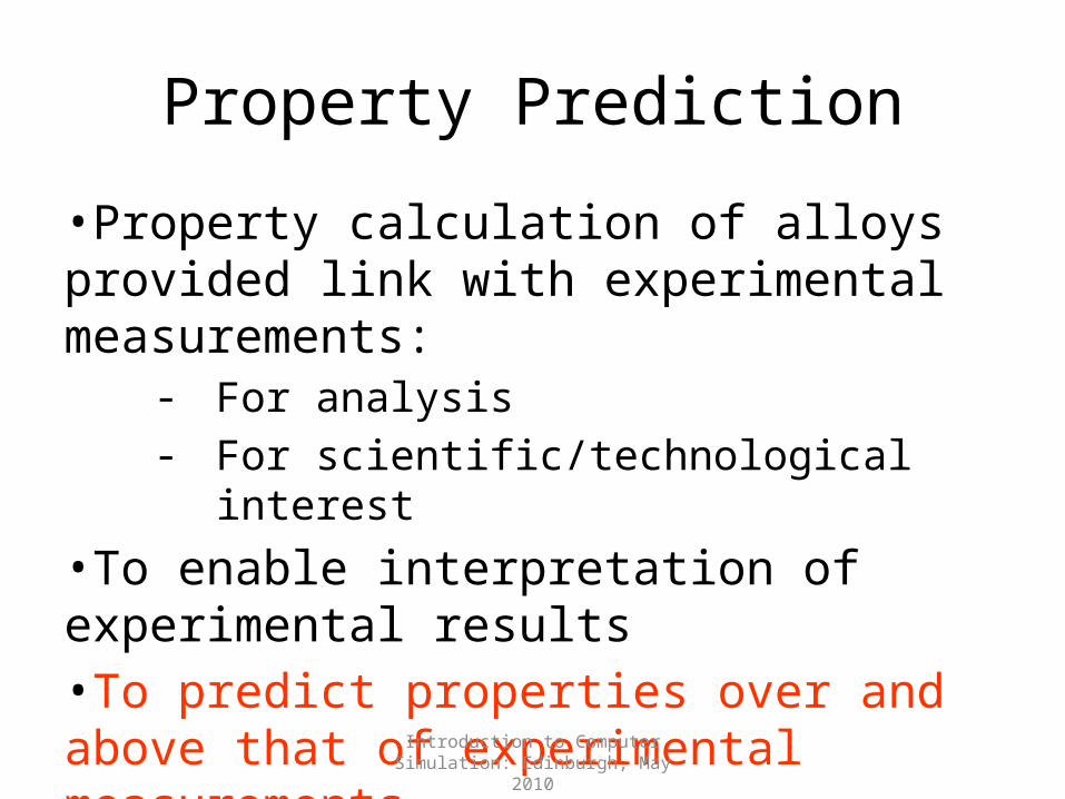
Property Prediction
•Property calculation of alloys provided link with experimental measurements:
- For analysis- For scientific/technological interest
•To enable interpretation of experimental results•To predict properties over and above that of experimental measurements
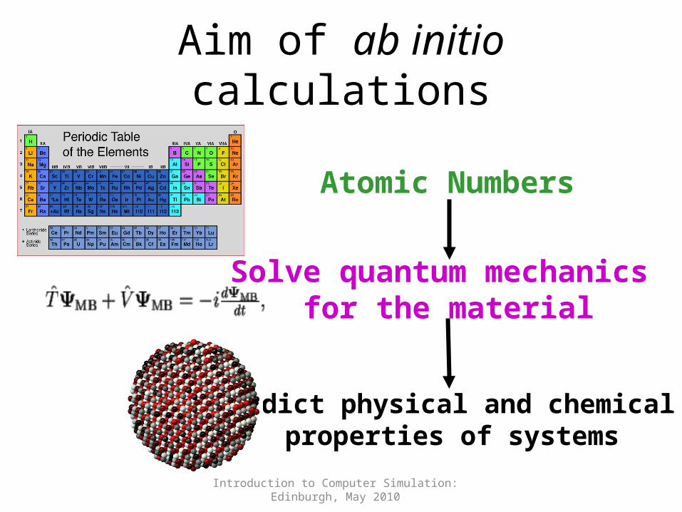
Aim of ab initio calculations
Introduction to Computer Simulation: Edinburgh, May 2010
Atomic Numbers
Solve quantum mechanics for the material
Predict physical and chemical properties of systems
Introduction to Computer Simulation: Edinburgh, May 2010
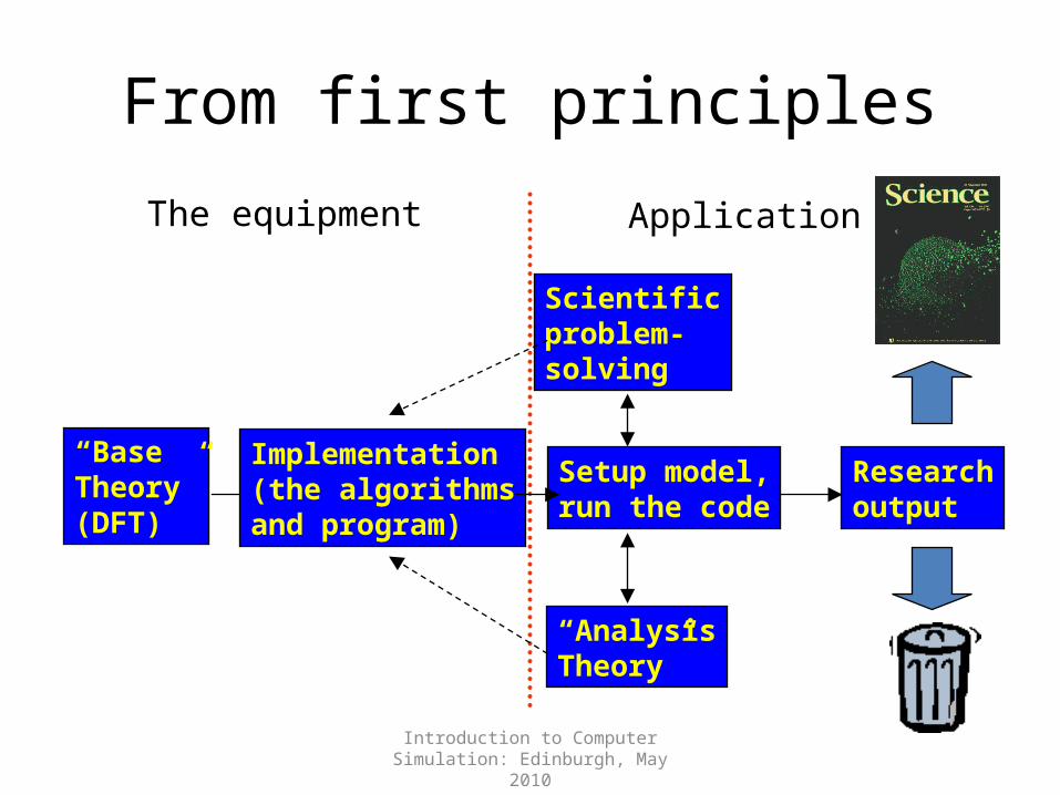
From first principles
Researchoutput
The equipment Application
“BaseTheory”(DFT)
Implementation(the algorithmsand program)
Setup model,run the code
Scientificproblem-solving
“AnalysisTheory”
Introduction to Computer Simulation: Edinburgh, May 2010
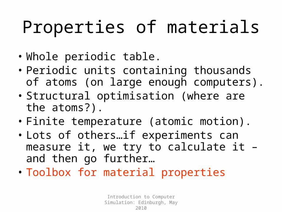
Properties of materials
• Whole periodic table.• Periodic units containing thousands of atoms
(on large enough computers).• Structural optimisation (where are the
atoms?).• Finite temperature (atomic motion).• Lots of others…if experiments can measure it,
we try to calculate it – and then go further…• Toolbox for material properties
Introduction to Computer Simulation: Edinburgh, May 2010
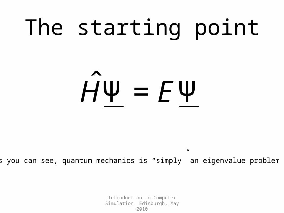
The starting point
€
ˆ H Ψ = EΨ
As you can see, quantum mechanics is “simply” an eigenvalue problem
Introduction to Computer Simulation: Edinburgh, May 2010
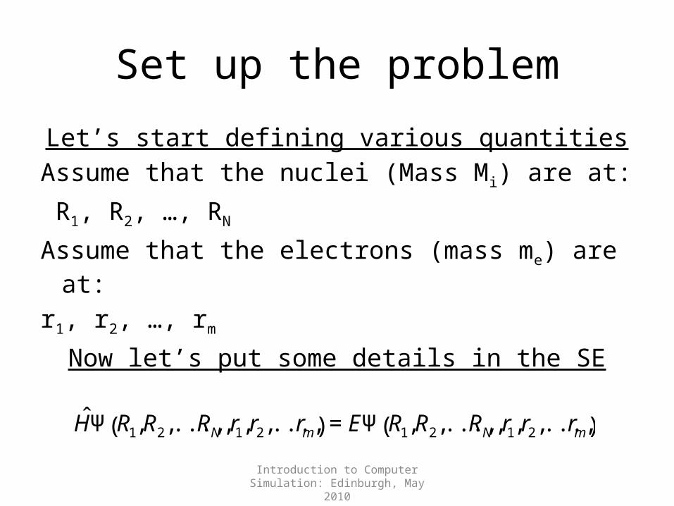
Set up the problem
Let’s start defining various quantitiesAssume that the nuclei (Mass Mi) are at: R1, R2, …, RN
Assume that the electrons (mass me) are at:r1, r2, …, rm
Now let’s put some details in the SE
€
ˆ H Ψ R1,R2,...,RN ,r1,r2,...,rm( ) = EΨ R1,R2,...,RN ,r1,r2,...,rm( )
Introduction to Computer Simulation: Edinburgh, May 2010
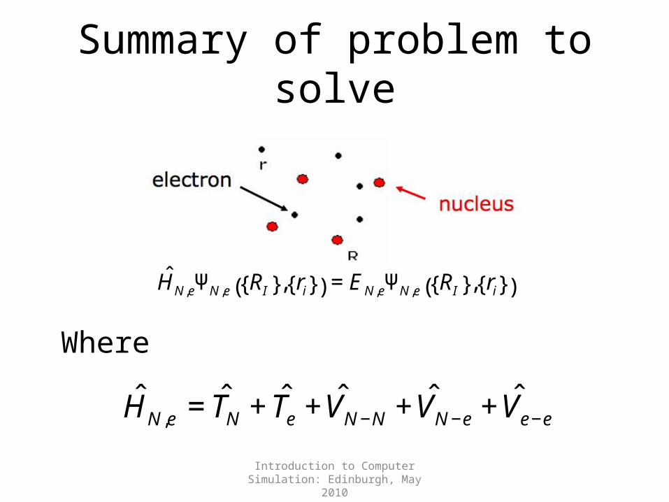
Summary of problem to solve
€
ˆ H N ,eΨN ,e RI{ }, ri{ }( ) = EN ,eΨN ,e RI{ }, ri{ }( )
Where
€
ˆ H N ,e = ˆ T N + ˆ T e + ˆ V N −N + ˆ V N −e + ˆ V e −e
Introduction to Computer Simulation: Edinburgh, May 2010
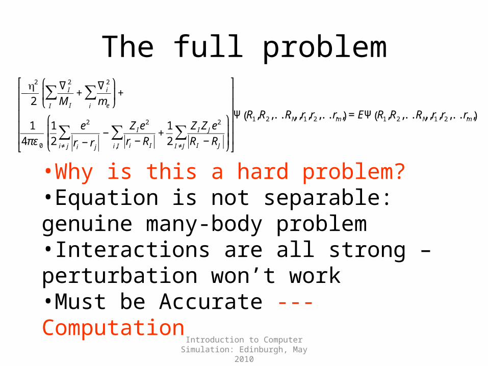
The full problem
€
−h2
2∇I
2
M II∑ +
∇ i2
mei∑
⎛
⎝ ⎜
⎞
⎠ ⎟+
14πε 0
12
e2
ri − rj
−ZIe
2
ri − RIi,I∑
i≠ j∑ +
12
ZI ZJe2
RI − RJI ≠J∑
⎛
⎝ ⎜ ⎜
⎞
⎠ ⎟ ⎟
⎡
⎣
⎢ ⎢ ⎢ ⎢ ⎢
⎤
⎦
⎥ ⎥ ⎥ ⎥ ⎥
Ψ R1,R2,...,RN ,r1,r2,...,rm( ) = EΨ R1,R2,...,RN ,r1,r2,...,rm( )
•Why is this a hard problem? •Equation is not separable: genuine many-body problem•Interactions are all strong – perturbation won’t work•Must be Accurate --- Computation
Introduction to Computer Simulation: Edinburgh, May 2010
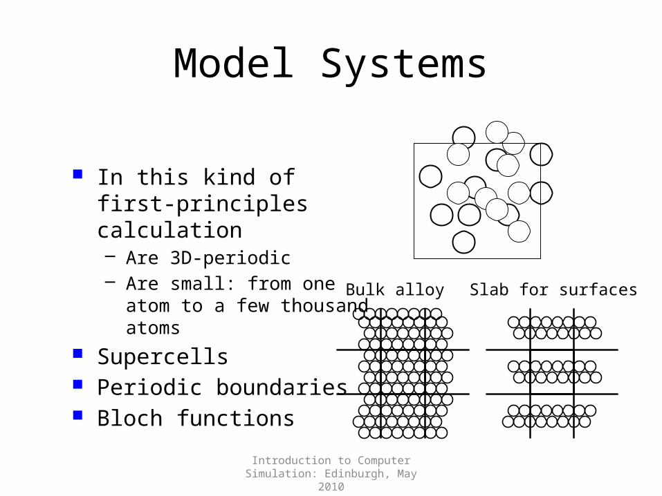
Model Systems
In this kind of first-principles calculation– Are 3D-periodic– Are small: from one atom to a few
thousand atoms Supercells Periodic boundaries Bloch functions
Bulk alloy Slab for surfaces
Introduction to Computer Simulation: Edinburgh, May 2010
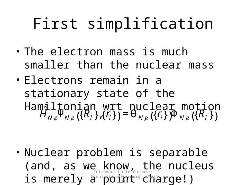
First simplification
• The electron mass is much smaller than the nuclear mass
• Electrons remain in a stationary state of the Hamiltonian wrt nuclear motion
• Nuclear problem is separable (and, as we know, the nucleus is merely a point charge!)
€
ˆ H N ,eΨN ,e RI{ }, ri{ }( ) = ΘN ,e ri{ }( )ΦN ,e RI{ }( )
Introduction to Computer Simulation: Edinburgh, May 2010
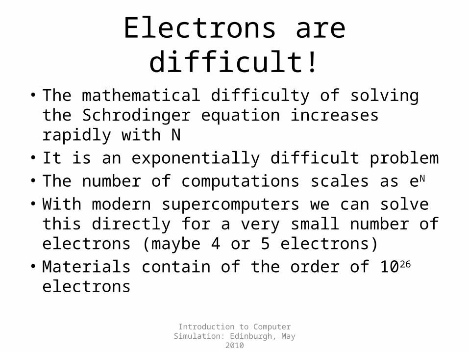
Electrons are difficult!
• The mathematical difficulty of solving the Schrodinger equation increases rapidly with N
• It is an exponentially difficult problem• The number of computations scales as eN
• With modern supercomputers we can solve this directly for a very small number of electrons (maybe 4 or 5 electrons)
• Materials contain of the order of 1026 electrons
Introduction to Computer Simulation: Edinburgh, May 2010
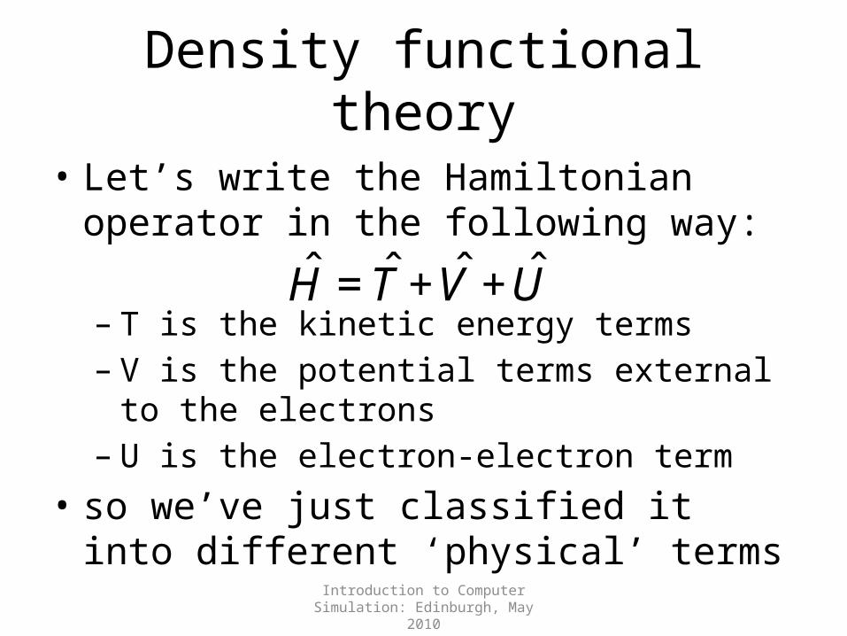
Density functional theory
• Let’s write the Hamiltonian operator in the following way:
– T is the kinetic energy terms– V is the potential terms external to the electrons– U is the electron-electron term
• so we’ve just classified it into different ‘physical’ terms€
ˆ H = ˆ T + ˆ V + ˆ U
Introduction to Computer Simulation: Edinburgh, May 2010
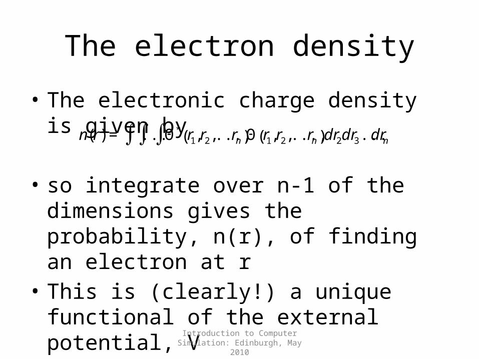
The electron density
• The electronic charge density is given by
• so integrate over n-1 of the dimensions gives the probability, n(r), of finding an electron at r
• This is (clearly!) a unique functional of the external potential, V
• That is, fix V, solve SE (somehow) for Q and then get n(r).
€
n(r) = ... Θ* r1,r2,...,rn( )∫∫∫ Θ r1,r2,...,rn( )dr2dr3 ...drn
Introduction to Computer Simulation: Edinburgh, May 2010
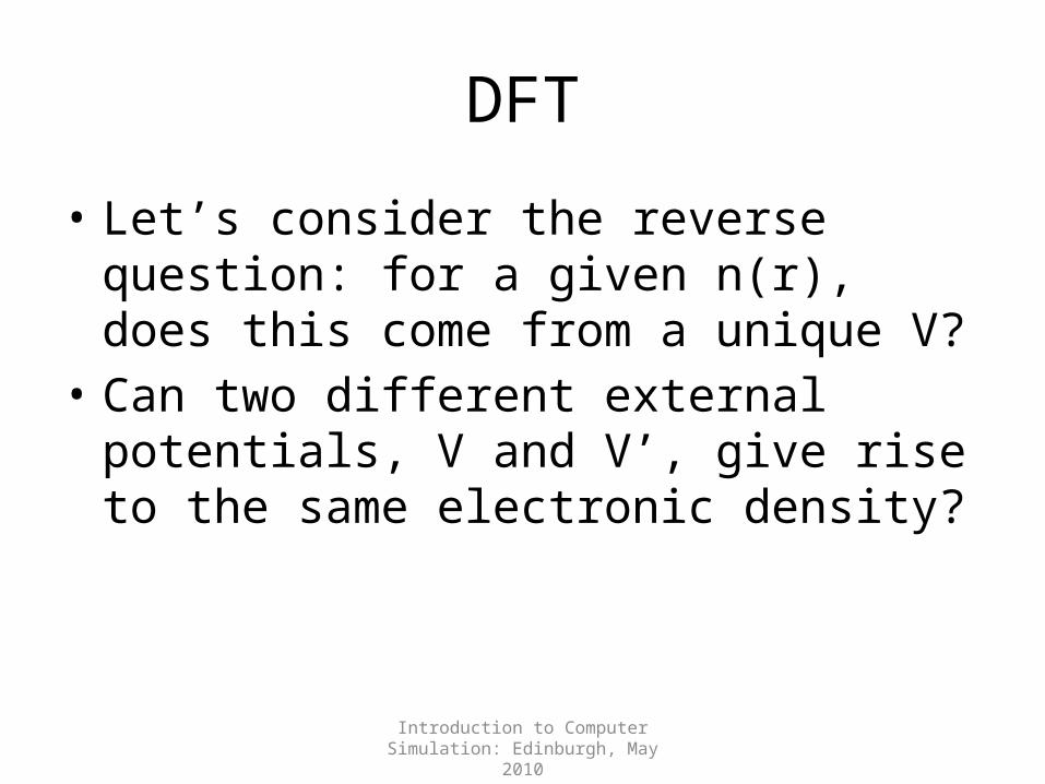
DFT
• Let’s consider the reverse question: for a given n(r), does this come from a unique V?
• Can two different external potentials, V and V’, give rise to the same electronic density?
Introduction to Computer Simulation: Edinburgh, May 2010
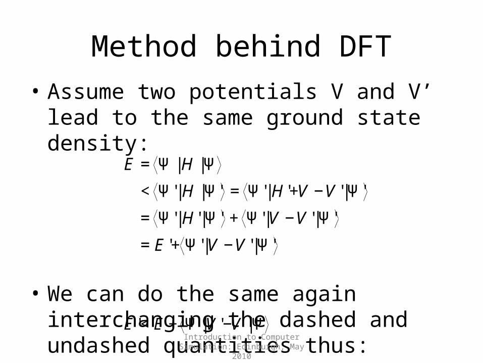
Method behind DFT• Assume two potentials V and V’ lead to the
same ground state density:
• We can do the same again interchanging the dashed and undashed quantities thus:€
E = Ψ | H | Ψ< Ψ'| H | Ψ' = Ψ'| H '+V −V ' | Ψ'= Ψ'| H ' | Ψ' + Ψ'|V −V ' | Ψ'= E '+ Ψ'|V −V ' | Ψ'
€
E ' < E + Ψ |V '−V | Ψ
Introduction to Computer Simulation: Edinburgh, May 2010
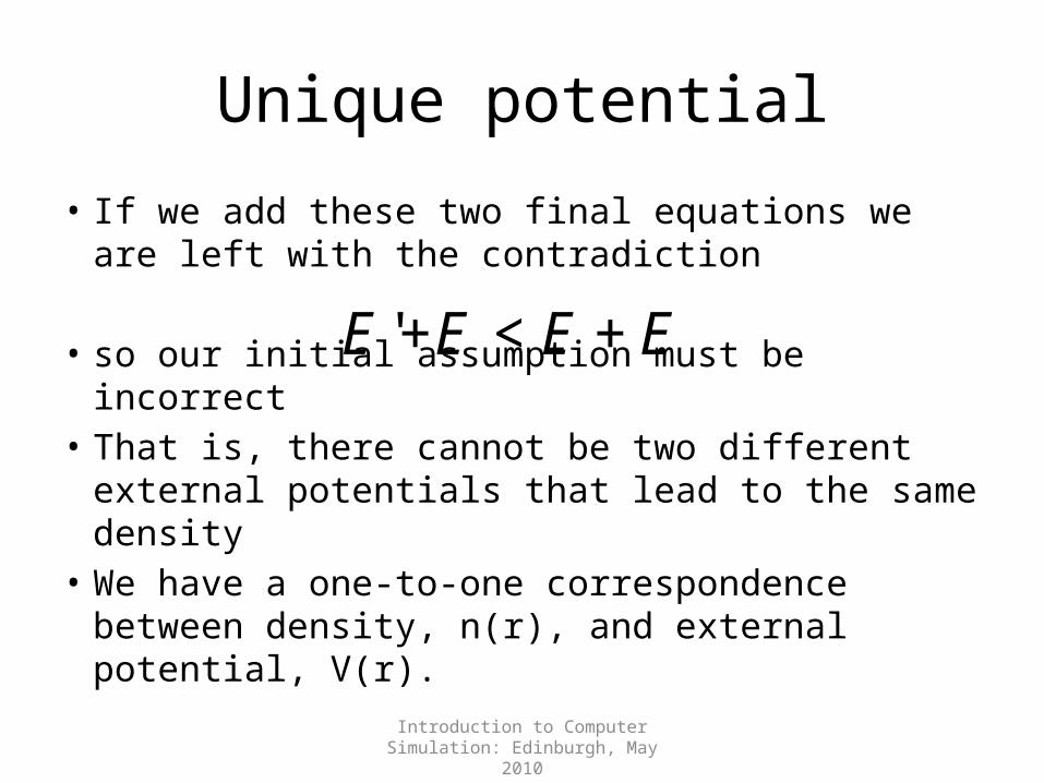
Unique potential
• If we add these two final equations we are left with the contradiction
• so our initial assumption must be incorrect• That is, there cannot be two different external
potentials that lead to the same density• We have a one-to-one correspondence between
density, n(r), and external potential, V(r).€
E '+E < E + E '
Introduction to Computer Simulation: Edinburgh, May 2010
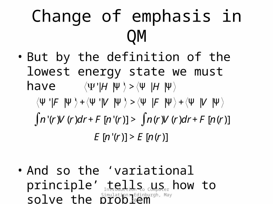
Change of emphasis in QM
• But by the definition of the lowest energy state we must have
• And so the ‘variational principle’ tells us how to solve the problem
€
Ψ' | H | Ψ' > Ψ | H | ΨΨ'| F | Ψ' + Ψ'|V | Ψ' > Ψ | F | Ψ + Ψ |V | Ψ
n'(r)V (r)dr + F n'(r)[ ]∫ > n(r)V (r)dr + F n(r)[ ]∫E n'(r)[ ] > E n(r)[ ]
Introduction to Computer Simulation: Edinburgh, May 2010
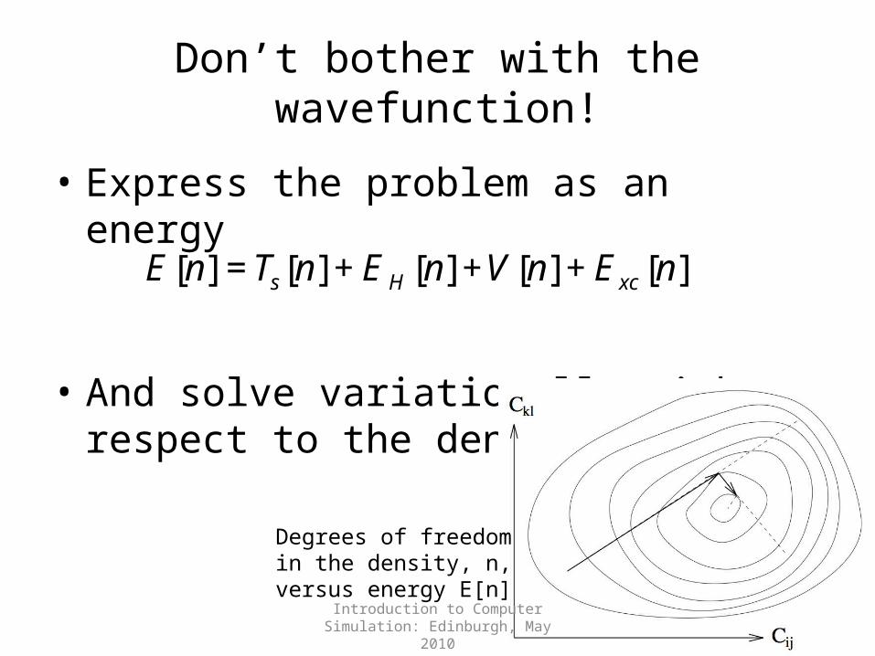
Don’t bother with the wavefunction!
• Express the problem as an energy
• And solve variationally with respect to the density
€
E n[ ] = Ts n[ ] + E H n[ ] +V n[ ] + Exc n[ ]
Degrees of freedomin the density, n, versus energy E[n]
Introduction to Computer Simulation: Edinburgh, May 2010
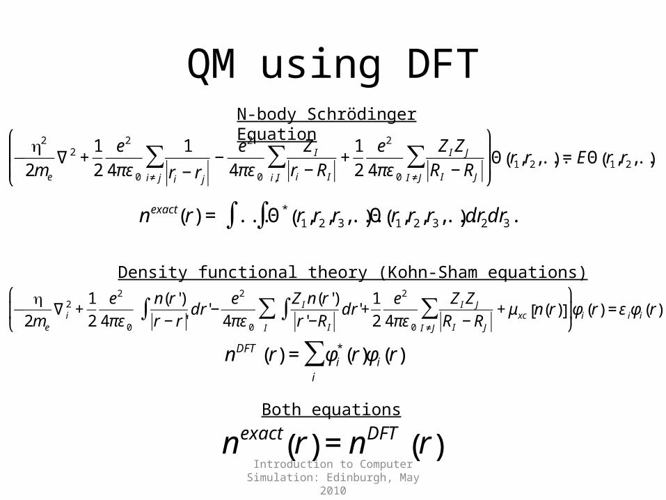
QM using DFT
€
−h2
2me
∇2 +12
e2
4πε 0
1ri − rj
−e2
4πε 0
ZI
ri − RIi,I∑
i≠ j∑ +
12
e2
4πε 0
ZI ZJ
RI − RJI ≠J∑
⎛
⎝ ⎜ ⎜
⎞
⎠ ⎟ ⎟Θ r1,r2,...( ) = EΘ r1,r2,...( )
€
n exact r( ) = ... Θ* r1,r2,r3,...( )Θ r1,r2,r3,...( )dr2dr3 ...∫∫
N-body Schrödinger Equation
€
−h
2me
∇ i2 +
12
e2
4πε 0
n(r')r − r'
dr' −e2
4πε 0
ZI n(r')r' −RI
dr'+12
e2
4πε 0
ZI ZJ
RI − RJI ≠J∑∫
I∑∫ + μ xc n r( )[ ]
⎛
⎝ ⎜
⎞
⎠ ⎟φi r( ) = ε iφi r( )
€
nDFT r( ) = φi* r( )φi r( )
i∑
€
n exact r( ) = nDFT r( )
Density functional theory (Kohn-Sham equations)
Both equations
Introduction to Computer Simulation: Edinburgh, May 2010
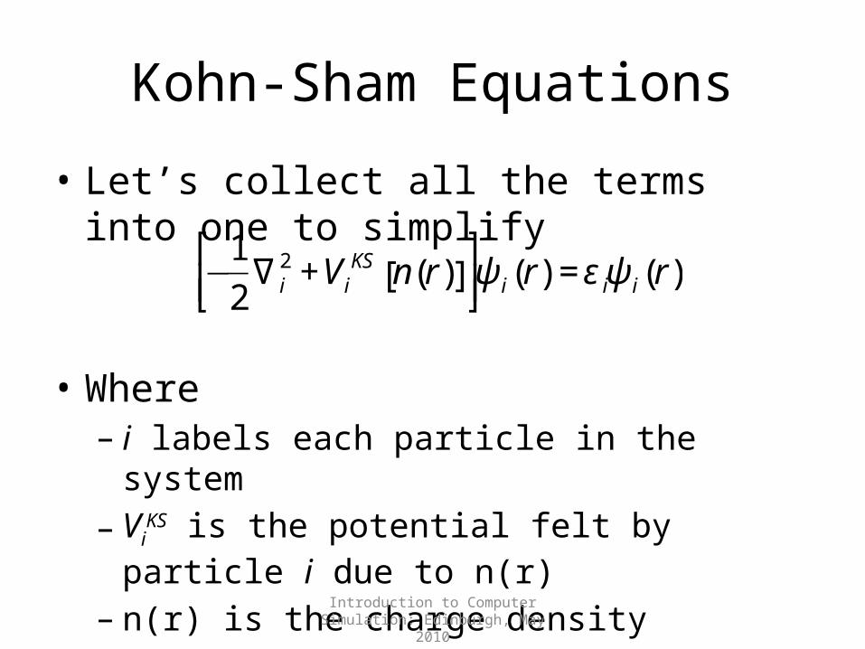
Kohn-Sham Equations
• Let’s collect all the terms into one to simplify
• Where– i labels each particle in the system– Vi
KS is the potential felt by particle i due to n(r)– n(r) is the charge density
€
−12
∇ i2 +Vi
KS n r( )[ ] ⎡ ⎣ ⎢
⎤ ⎦ ⎥ψ i r( ) = ε iψ i r( )
Introduction to Computer Simulation: Edinburgh, May 2010
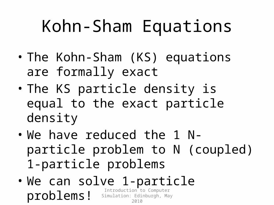
Kohn-Sham Equations
• The Kohn-Sham (KS) equations are formally exact
• The KS particle density is equal to the exact particle density
• We have reduced the 1 N-particle problem to N (coupled) 1-particle problems
• We can solve 1-particle problems!
Introduction to Computer Simulation: Edinburgh, May 2010
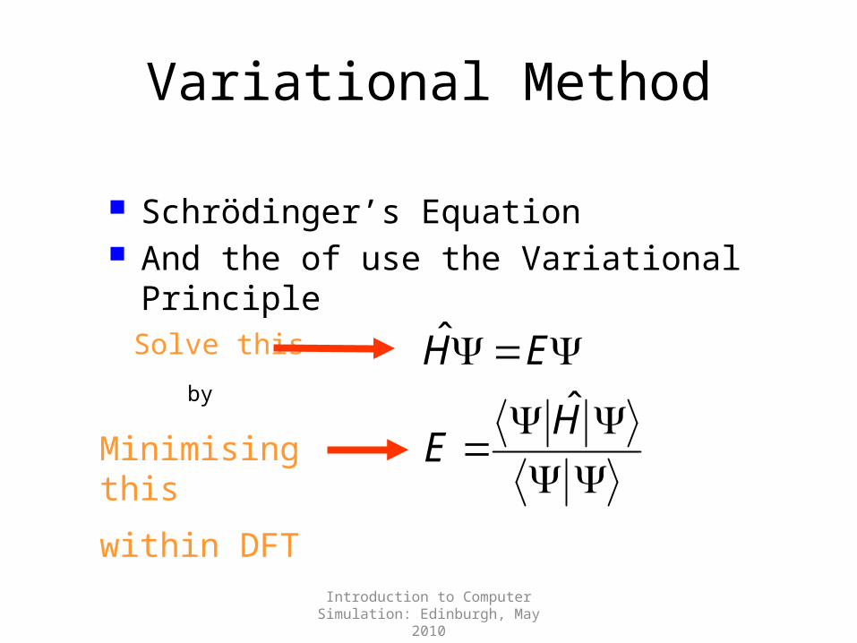
Variational Method
Schrödinger’s Equation And the of use the Variational Principle
ˆ H ΨEΨ
E Ψ ˆ H ΨΨ Ψ
Minimising this
within DFT
Solve this
by
Introduction to Computer Simulation: Edinburgh, May 2010
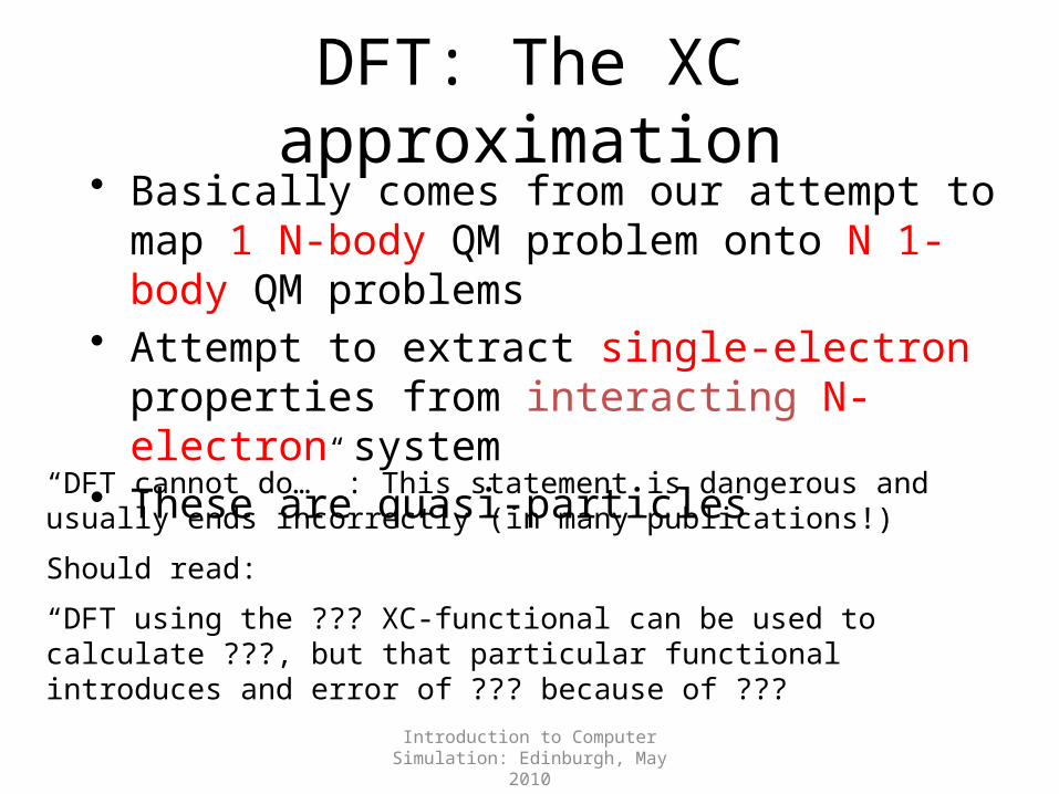
DFT: The XC approximation• Basically comes from our attempt to map 1 N-body
QM problem onto N 1-body QM problems• Attempt to extract single-electron properties from
interacting N-electron system• These are quasi-particles
“DFT cannot do…” : This statement is dangerous and usually ends incorrectly (in many publications!)
Should read:
“DFT using the ??? XC-functional can be used to calculate ???, but that particular functional introduces and error of ??? because of ???
Introduction to Computer Simulation: Edinburgh, May 2010
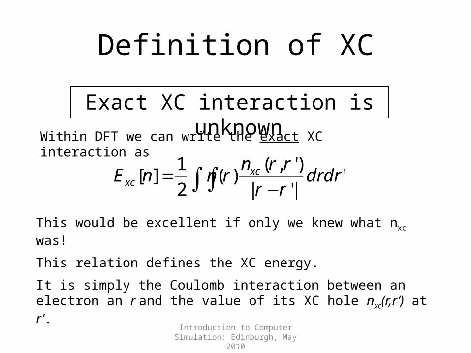
Definition of XC
Exact XC interaction is unknown
∫∫ − '
|'|)',()(
21][ drdr
rrrrnrnnE xc
xc
This would be excellent if only we knew what nxc was!
This relation defines the XC energy.
It is simply the Coulomb interaction between an electron an r and the value of its XC hole nxc(r,r’) at r’.
Within DFT we can write the exact XC interaction as
Introduction to Computer Simulation: Edinburgh, May 2010
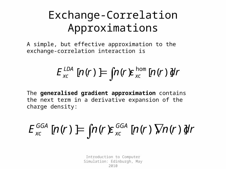
Exchange-Correlation Approximations
∫ drrnrnrnE xcLDAxc )]([)()]([ homε
∫ ∇ drrnrnrnrnE GGAxc
GGAxc )](),([)()]([ ε
A simple, but effective approximation to the exchange-correlation interaction is
The generalised gradient approximation contains the next term in a derivative expansion of the charge density:
Introduction to Computer Simulation: Edinburgh, May 2010
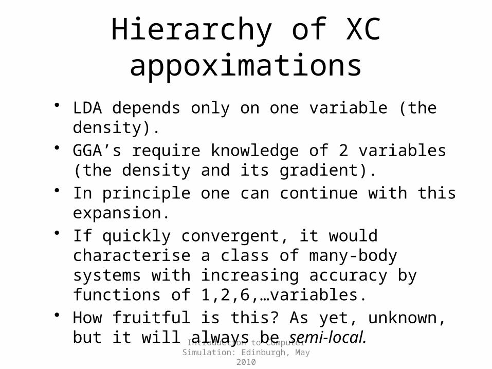
Hierarchy of XC appoximations
• LDA depends only on one variable (the density).• GGA’s require knowledge of 2 variables (the density and
its gradient).• In principle one can continue with this expansion.• If quickly convergent, it would characterise a class of
many-body systems with increasing accuracy by functions of 1,2,6,…variables.
• How fruitful is this? As yet, unknown, but it will always be semi-local.
Introduction to Computer Simulation: Edinburgh, May 2010
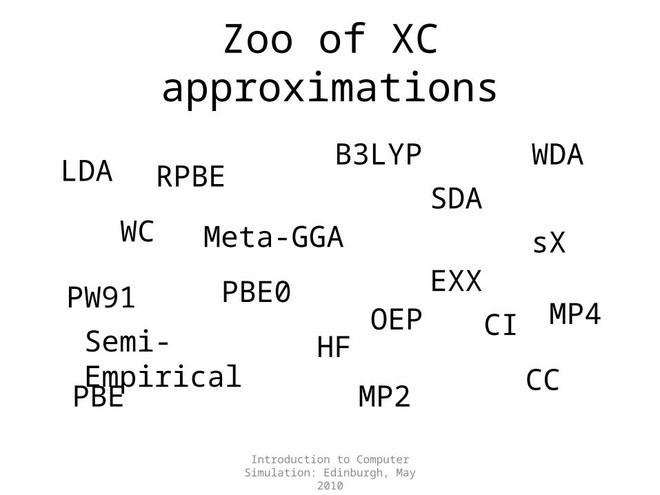
Zoo of XC approximations
LDA
Semi-Empirical
RPBE
WC
WDA
CIPW91
PBE
EXXsX
CC
B3LYP
PBE0
Meta-GGA
HF
MP2
MP4
SDA
OEP
Introduction to Computer Simulation: Edinburgh, May 2010
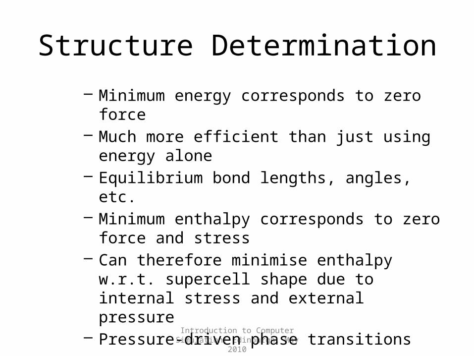
Structure Determination– Minimum energy corresponds to zero force– Much more efficient than just using energy
alone– Equilibrium bond lengths, angles, etc.– Minimum enthalpy corresponds to zero
force and stress– Can therefore minimise enthalpy w.r.t.
supercell shape due to internal stress and external pressure
– Pressure-driven phase transitions
Introduction to Computer Simulation: Edinburgh, May 2010
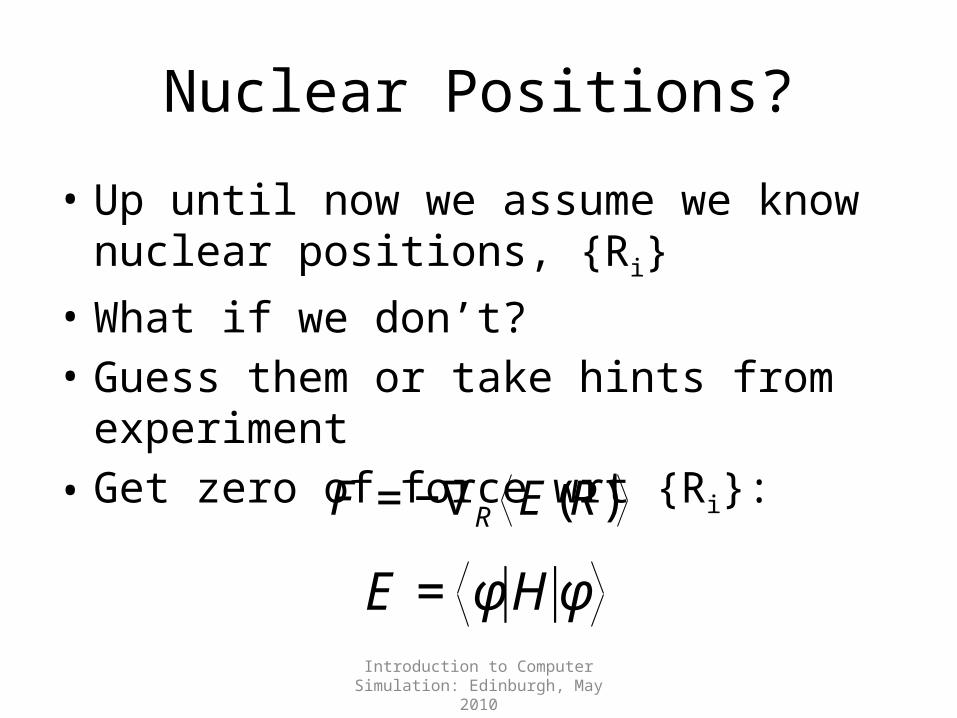
Nuclear Positions?
• Up until now we assume we know nuclear positions, {Ri}
• What if we don’t?• Guess them or take hints from experiment• Get zero of force wrt {Ri}:
€
F = −∇R E(R)
€
E = φ H φ
Introduction to Computer Simulation: Edinburgh, May 2010
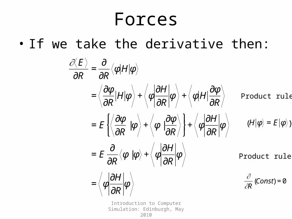
Forces• If we take the derivative then:
€
∂ E∂R
=∂
∂Rφ H φ
=∂φ∂R
H φ + φ∂H∂R
φ + φ H∂φ∂R
= E∂φ∂R
| φ + φ |∂φ∂R
⎧ ⎨ ⎩
⎫ ⎬ ⎭+ φ
∂H∂R
φ
= E∂
∂Rφ | φ + φ
∂H∂R
φ
= φ∂H∂R
φ
€
H φ = E φ( )
Product rule
Product rule
€
∂∂R
Const( ) = 0
Introduction to Computer Simulation: Edinburgh, May 2010
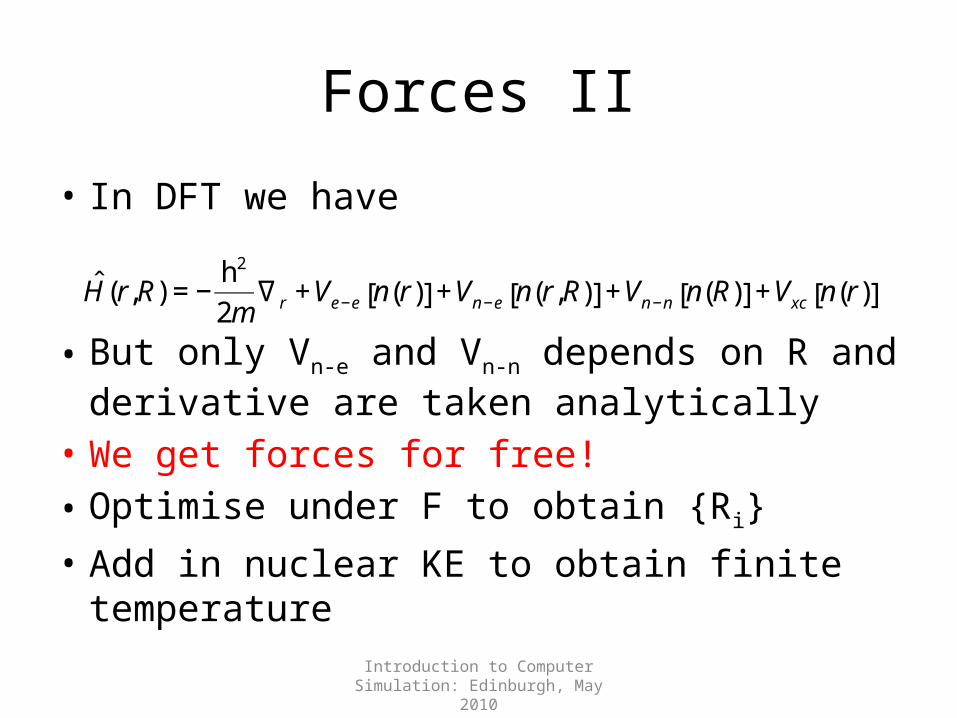
Forces II
• In DFT we have
• But only Vn-e and Vn-n depends on R and derivative are taken analytically
• We get forces for free!• Optimise under F to obtain {Ri}• Add in nuclear KE to obtain finite temperature
€
ˆ H (r,R) = −h2
2m∇r +Ve −e n r( )[ ] +Vn −e n r,R( )[ ] +Vn −n n R( )[ ] +Vxc n r( )[ ]
Introduction to Computer Simulation: Edinburgh, May 2010
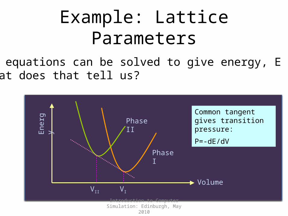
Example: Lattice Parameters
Volume
Ener
gy
Phase I
Phase IICommon tangent gives transition pressure:
P=-dE/dV
VII VI
•KS equations can be solved to give energy, E•What does that tell us?
Introduction to Computer Simulation: Edinburgh, May 2010
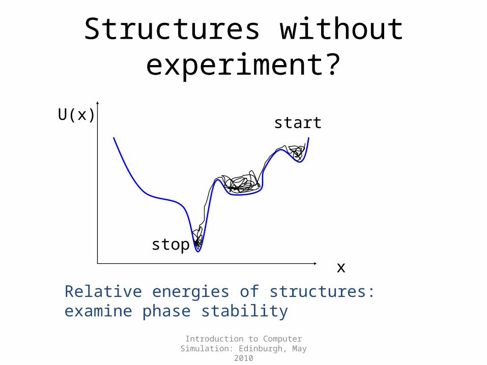
Structures without experiment?
U(x)
x
start
stop
Relative energies of structures: examine phase stability
Introduction to Computer Simulation: Edinburgh, May 2010
Summary so far
• Can get electronic density and energy• Can use forces (and stresses) to optimise
structure from an “intelligent” initial guess• Minima of energy gives structural phase
information
Introduction to Computer Simulation: Edinburgh, May 2010
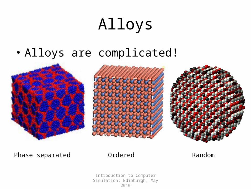
Alloys
• Alloys are complicated!
Phase separated Ordered Random
Introduction to Computer Simulation: Edinburgh, May 2010
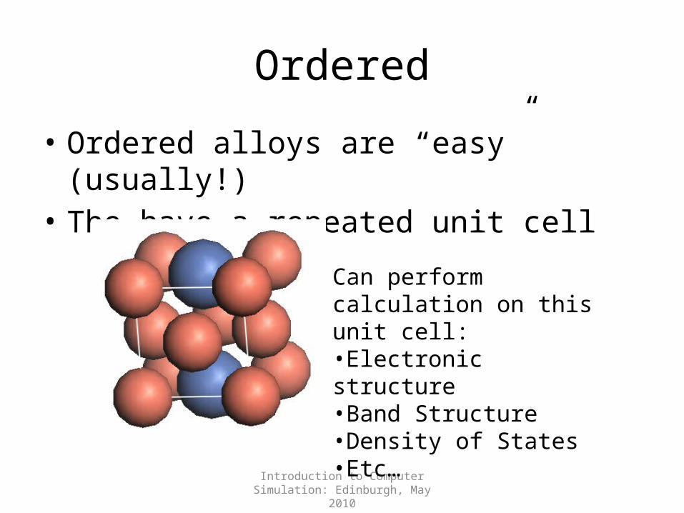
Ordered
• Ordered alloys are “easy” (usually!)• The have a repeated unit cell
Can perform calculation on this unit cell:•Electronic structure•Band Structure•Density of States•Etc…
Introduction to Computer Simulation: Edinburgh, May 2010
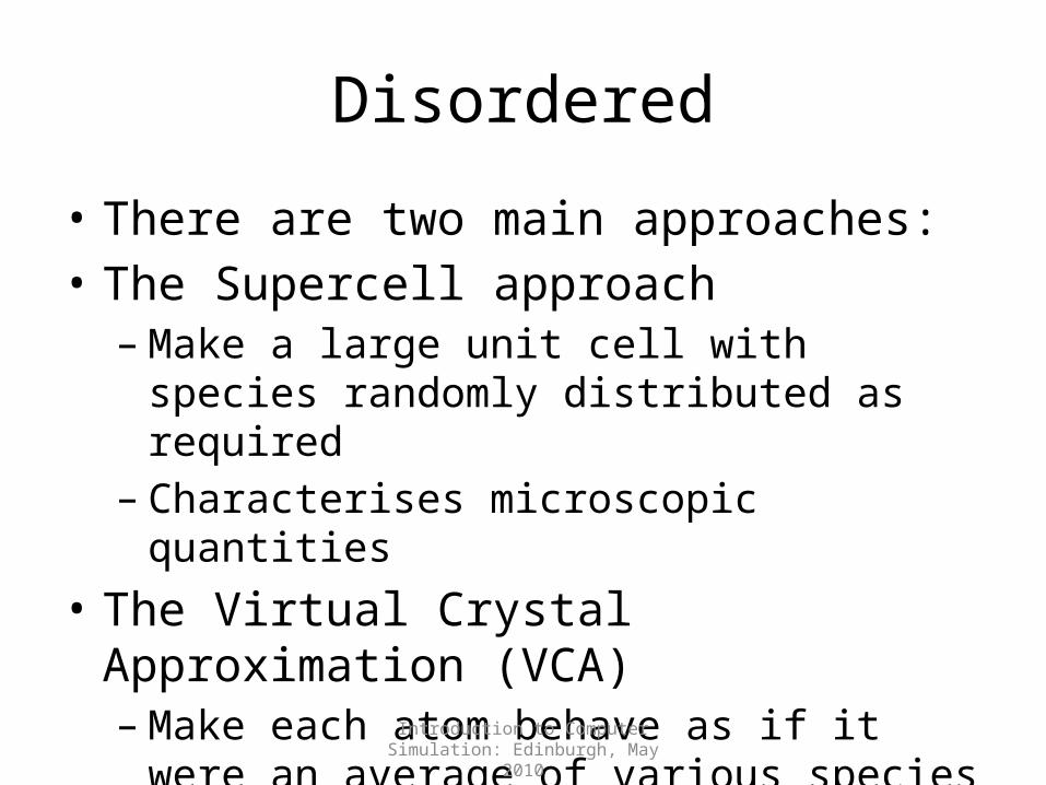
Disordered
• There are two main approaches:• The Supercell approach– Make a large unit cell with species randomly
distributed as required– Characterises microscopic quantities
• The Virtual Crystal Approximation (VCA)– Make each atom behave as if it were an average of
various species AxB1-x
– Encapsulates only average quantities
Introduction to Computer Simulation: Edinburgh, May 2010
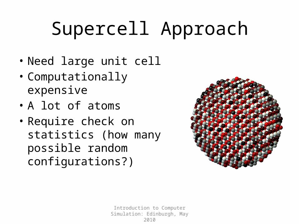
Supercell Approach
• Need large unit cell• Computationally
expensive• A lot of atoms• Require check on
statistics (how many possible random configurations?)
Introduction to Computer Simulation: Edinburgh, May 2010
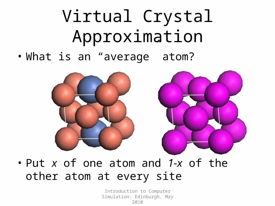
Virtual Crystal Approximation
• What is an “average” atom?
• Put x of one atom and 1-x of the other atom at every site
Introduction to Computer Simulation: Edinburgh, May 2010
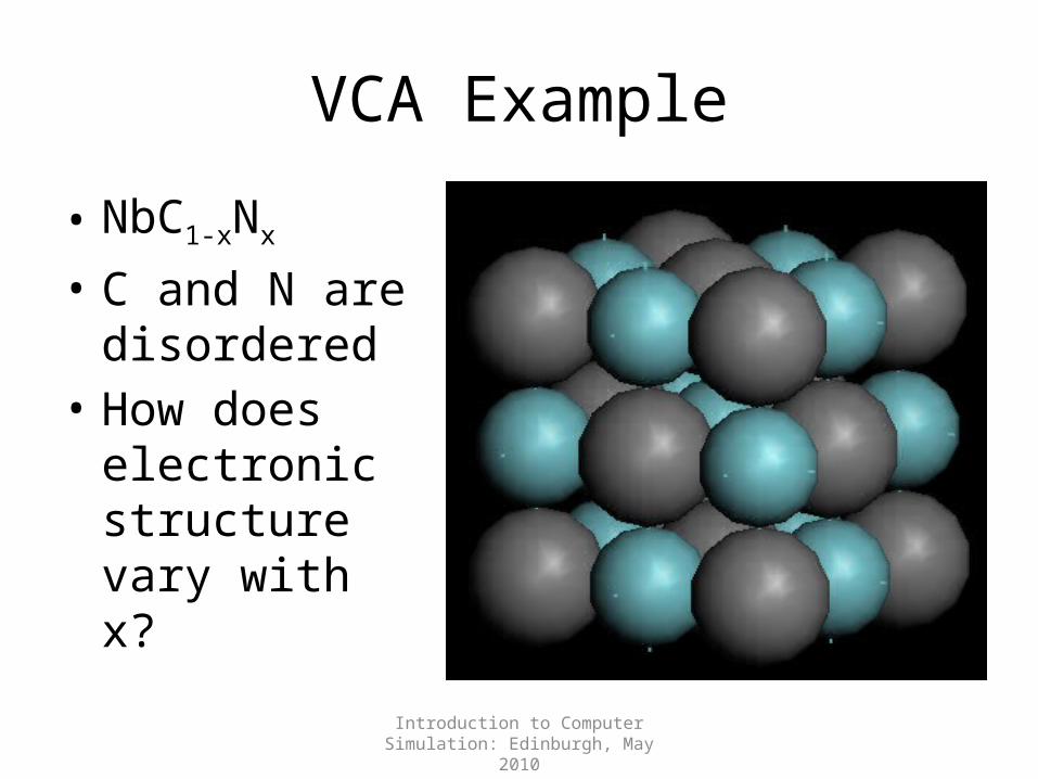
VCA Example
• NbC1-xNx
• C and N are disordered
• How does electronic structure vary with x?
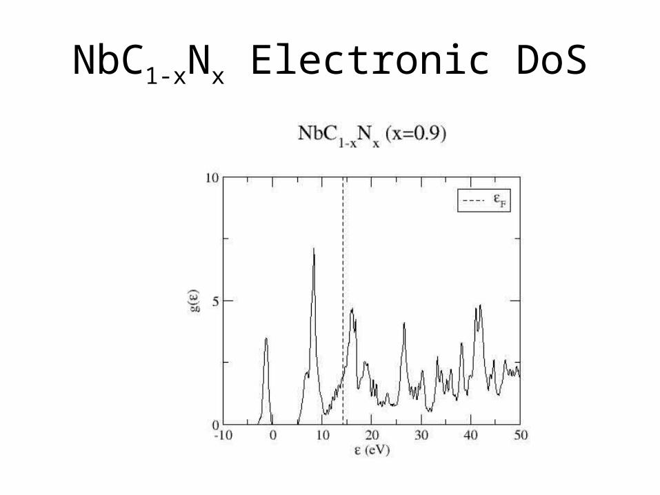
Introduction to Computer Simulation: Edinburgh, May 2010
NbC1-xNx Electronic DoS
Introduction to Computer Simulation: Edinburgh, May 2010
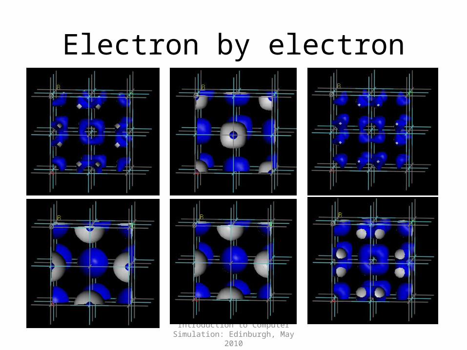
Electron by electron
Introduction to Computer Simulation: Edinburgh, May 2010
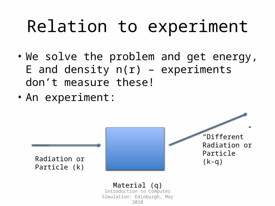
Relation to experiment
• We solve the problem and get energy, E and density n(r) – experiments don’t measure these!
• An experiment:
Radiation orParticle (k)
Material (q)
“Different”Radiation orParticle(k-q)
Introduction to Computer Simulation: Edinburgh, May 2010
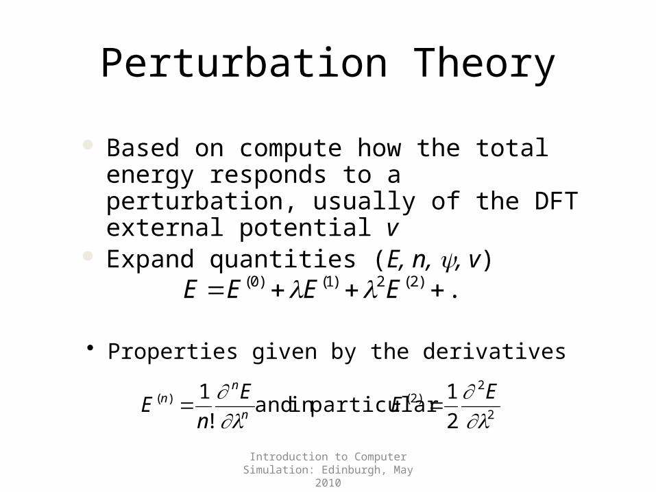
Perturbation Theory
Based on compute how the total energy responds to a perturbation, usually of the DFT external potential v
Expand quantities (E, n, y, v)
...)2(2)1()0( EEEE
• Properties given by the derivatives
2
2)2()(
21particularin and
!1
EEE
nE n
nn
Introduction to Computer Simulation: Edinburgh, May 2010
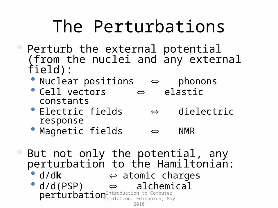
The Perturbations Perturb the external potential (from the nuclei and
any external field):• Nuclear positions phonons• Cell vectors elastic constants• Electric fields dielectric response• Magnetic fields NMR
But not only the potential, any perturbation to the Hamiltonian:• d/dk atomic charges• d/d(PSP) alchemical perturbation
Introduction to Computer Simulation: Edinburgh, May 2010
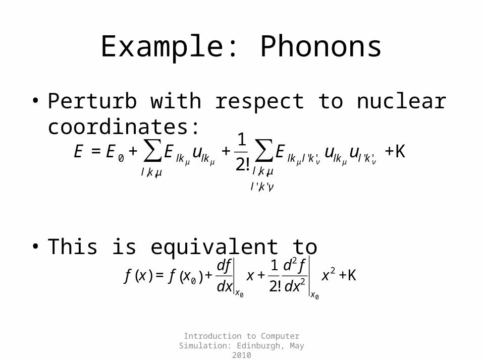
Example: Phonons
• Perturb with respect to nuclear coordinates:
• This is equivalent to
€
E = E0 + E lk μulk μ
l,k,μ∑ +
12!
E lk μ l 'k 'νulk μ
ul 'k'ν+K
l,k,μl ',k ',ν
∑
€
f (x) = f x0( ) +dfdx x0
x +12!
d2 fdx 2
x0
x 2 +K
Introduction to Computer Simulation: Edinburgh, May 2010
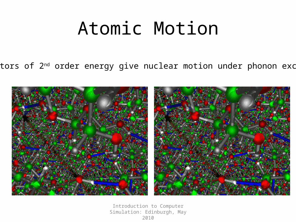
Atomic Motion
Eigenvectors of 2nd order energy give nuclear motion under phonon excitations
Introduction to Computer Simulation: Edinburgh, May 2010
Summary• First principles electronic structure calculations:
Extremely powerful technique in condensed matter• Applicable to many different sciences
Condensed Matter Physics Chemistry Biology Material Science Surfaces Geology
• Simulate experimental measurements• Computationally possible, but still requires good
computer resources