Quantum Information Theory - Block 2 - 2015 - ku · PDF fileQuantum Information Theory - Block...

Quantum Information Theory - Block 2 - 2015

Matthias Christandl

January 14, 2016

Contents

1 Organisation and Historic Remarks 2

2 Lecture 1: Probability Theory 3

3 Lecture 2: Data Compression 6

4 Lecture 3: Vectors and Operators 11

5 Lecture 4: Quantum Channels and the Formalism of QuantumInformation Theory 15

6 Lecture 5: The Choi-Jamilkowski isomorphism 18

7 Lecture 6: Stinespring and Kraus 19

8 Lecture 7: Measurements 21

9 Lecture 8: Teleportation 23

10 Lecture 9: Superdense Coding and Distances 25

11 Lecture 10: Quantum Data Compression 28

12 Lecture 11: Quantum Entropy 30

13 Lecture 12: The Decoupling Theorem 34

14 Lecture 13: Quantum State Merging: Part I 37

15 Lecture 14: State Merging Part II 39

1

1 Organisation and Historic Remarks

The course will run for seven weeks with a 20min oral examination at the end.There are 2-hour lectures on Tuesday and on Thursday morning each withexercises given by Christian Majenz on Thursday afternoon. Every Tuesday forthe first 6 weeks, an exercise sheet will be handed out, which is to be returnedthe following Tuesday. It will then be marked and returned to you in the exerciselesson in the same week.

I will try to hand out lecture notes every week. As additional material, Irecommend the book Quantum Information and Computation by Nielsen andChuang as well as the book by Mark Wilde. I also recommend online lecturenotes by John Preskill (Caltech), John Watrous (Waterloo) and Renato Renner(ETH Zurich).

In the 1930’s and 1940’s, Turing and Shannon abstracted the concept ofinformation from its physical carrier with the goal of a universal theory ofinformation and computation that would apply to all physical systems.

Their theories, however, are based on the idea that information always existsand that our ignorance about it is only of a technical and not a fundamentalnature. Their theories are therefore based on classical physics and it can beshown that they do not allow to abstract information in quantum systems thatare described by quantum theory.

Quantum theory was developed in the first half of the 20th century. Whereasearly on, in the 1930s, unexpected information-theoretic properties of quantumtheory came to light (e.g. EPR paradox, Schroedinger’s cat), only in the secondhalf, in the light of experimental progress in the manipulation of quantum sys-tems, did the development of a theory of quantum information and computationaccelerate.

It is this theory, focused not on its computational but rather on its informa-tional aspects, that we will develop in this course.

2

2 Lecture 1: Probability Theory

Let X be a random variable with range X = {0, . . . , d − 1} (all ranges in thiscourse will be finite and thus the labeling is mostly immaterial) and (probability)distribution

P : X → R+,

i.e. P (x) ≥ 0 for all x ∈ X , and∑x∈X P (x) = 1. We denote the size of X by

|X | = d. If we relax the last constraint to∑x∈X P (x) ≤ 1 we speak of a subnor-

malised (probability) distribution. We will often consider sources that spit outsymbols x distributed according to the distribution P and depict them as follows:

Source x

A pair of random variables (X,Y ) with range X ×Y has a joint distribution

PXY : X × Y → R+.

We will often think about a source that emits two symbols that are correlated:

Sourcexy

X is then distributed according to the marginal (probability) distribution

PX (x) :=∑y

PXY(x, y)

and similarly Y is distributed according to PY(y) :=∑x PXY(xy).

Often, it is important to study a value, conditioned on a second one. The dis-tribution of X conditioned on Y = y is the conditional (probability) distributiongiven by

PX|Y(x|y) = PXY(x, y)/PY(y)

if PY(y) > 0.Two random variables X and Y are independent if

PXY(x, y) = PX (x)PY(y).

Understanding when two distributions are close is very important in infor-mation theory. We therefore define the statistical distance of two distributionsP or Q both with range X by

δ(P,Q) :=1

2

∑x∈X|P (x)−Q(x)|.

In the exercise, you will see that the distance has an operational meaning in thesense that it corresponds to the bias when trying to distinguish P from Q afterhaving seen a single sample.

3

A channel is a probabilistic mapping from X to Y given by a conditionalprobability distribution PY|X .

x Channel y

The channel is deterministic if PY|X (y|x) := δy,f(x) for some function f :X → Y.

01−ε //

ε

&&

0

11−ε //

ε

88

1Channels can model noise as for instance in the binary symmetric channel.

Here, X = Y = 0, 1 and (dropping subscripts) P (0|0) = P (1|1) = 1 − ε andP (0|1) = P (1|0) = ε. Channels can also model computation as for instancein the CNOT gate. Here X = Y = 00, 01, 10, 11 and P (00|00) = P (01|01) =P (10|11) = P (11|10) = 1 and zero otherwise.

00 // 00

01 // 01

10

''

10

11

77

11When a symbol x emitted from a source with distribution PX enters the

channel, the symbol y that leaves the channel is distributed according to∑x

PX (x)PY|X (y|x).

Source x Channel y

The uncertainty contained in a probability distribution can be quantifiedwith help of entropies.

The most basic measures are the log of the support of the distribution (alsoknown as Renyi entropy of order 0)

H0(P ) := log |{x : P (x) > 0}|

and the negative log of the maximal value (also known as Renyi entropy of order∞)

H∞(P ) := − log maxx

P (x).

The most well-known, but already quite sophisticated measure is the Shannonentropy

H(P ) =∑x

P (x) log1

P (x)

4

which may be interpreted as the expected suprisal of the outcome. Wherethe surprisal of an outcome is the number of bits needed to write down theprobability of the outcome, log 1

P (x) . The entropies are all part of a series of

entropies, known as Renyi α entropies

Hα(P ) :=1

1− αlog(

∑x

P (x)α).

The Shannon entropy is the Renyi entropy of order 1.

5

3 Lecture 2: Data Compression

Imagine that we want to store a symbol emitted by a source but that storageis costly (and paid for, per bit). Then we want to find an encoder (a channel)that maps alphabet X to a smaller alphabet Y, such that there is a decoderthat maps Y back to X with the property that

Source x Encoder y Decoder x′

equals

Source x

Denoting the source distribution by PX (x) and the encoding and decod-ing maps by conditional distribution P encY|X (y|x) and P decX|Y(x|y) this requirementreads

Prob[x = dec ◦ enc(x)] =∑x,y,x′

P (x)P enc(y|x)P dec(x′|y)δx,x′ = 1 (1)

More formally, we want to compute the minimal storage cost

C(p) := min log |Y|

where the minimum is taken over all encoders and decoders such that (1) holds.What is the size of the minimal Y? Let us look at the probability distribution

of the source:

0 1 2 3

0

0.2

0.4

Clearly, the encoder can throw away (that is, map to the first symbol kept)all symbols that do not appear, that is, have p(x) = 0. But the encoder alsoneeds to keep at least a number of symbols that corresponds to the number ofsymbols that have the possibility to be emitted by the source. Otherwise, therewould be two such symbols x that are mapped to the same y. But then nodecoder could decide to which one to decode and (1) would not be satisfied. Agood encoder-decoder pair for our example is thus:

6

0 // 0

1

88

1

2

88

2

3

88

0 // 0

1

&&

1

2

&&

2

3Exercise: show that wlog encoder and decoder can be taken to be determin-

istic. Thus we have proved:

Theorem 1.C(p) = H0(p) := log suppp

where suppp := #{x : p(x) > 0}.

What if we are happy to tolerate a small error ε > 0? I.e. we relax (1) to

Prob[x = dec ◦ enc(x)] =∑x,y,x′

P (x)P enc(y|x)P dec(x′|y)δx,x′ ≥ 1− ε. (2)

Instead of throwing out the symbols that do not appear at all, we now throwaway the largest set of symbols S whose total probability is smaller than ε.

We obtain the following immediate corollary

Corollary 2.Cε(p) = Hε

0(p)

where Hε0(p) := minH0(q) where we minimize over all (non-normalised) distri-

butions q(x) ≤ p(x) with∑x q(x) ≥ 1− ε.

In the above example, the storage cost decreases when ε ≥ 0.2, 0.5, 0.7 and0.8. A more extreme example is given by the following distribution

0 1 2...

10

0

0.2

0.4

0.6

0.8

7

which shows that even a small ε (here ≥ 0.1) can lead to an arbitrary savingin storage space.

In the following we will consider the following special case, in which thesource consists of n independent and identical sources, and consider the storagecost per source, the rate for asymptotically vanishing error

R(p) := limε→0

limn→∞

1

nCε(pn)

In other words, we are looking to design an encoder Xn 7→ Y and decoderY 7→ Xn with minimal log |Y| and vanishing error as n gets large.

It follows immediately from the above that

Corollary 3.

R(p) = limε→0

limn→∞

1

nHε

0(pn).

It remains to find a simple formula for the RHS that does not involve thetwo limits, a single-letter formula, which can then be regarded as the solutionto this coding problem and is originally due to Shannon. Note that the stringof symbols xn := x1 . . . xn is identically and independently distributed (i.i.d.).

Looking at the following example, where the source emits three symbols,each distributed such 0 has probability 1/3 and 1 probability 2/3

000 001 010 100 011 101 110 111

0.1

0.2

0.3

we see that some strings have very low probability. More important, however,is the observation that the probability of the observed frequency is peaked. Theobserved frequency of the string, that is, the number of 0’s, 1’s, etc. is formallygiven by

f(xn) = (fxn(0), · · · fxn(d− 1))

wherefxn(x′) := #{j : xj = x′}.

It follows from the law of large numbers that the empirical distribution f (theobserved frequency divided by n) converges whp to the actual distribution p:

limn→∞

Prob[|||fxn − p||1 > δ] = 0.

8

where, more precisely,∑xn

p(x1) · · · p(xn)Θ(|||fxn − p||1 − δ > 0)

for Θ the heaviside step function. The 1-norm of a d-dimensional real vector gis defined by ||g||1 =

∑x′∈X |g(x′)|.

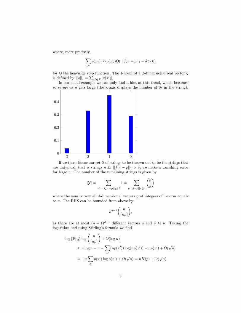
In our small example we can only find a hint at this trend, which becomesso severe as n gets large (the x-axis displays the number of 0s in the string):

3 2 1 00

0.1

0.2

0.3

0.4

If we thus choose our set S of strings to be thrown out to be the strings thatare untypical, that is strings with ||fxn − p||1 > δ, we make a vanishing errorfor large n. The number of the remaining strings is given by

|Y| =∑

xn:||fxn−p||1≤δ

1 =∑

g:||g−p||1≤δ

(n

g

)

where the sum is over all d-dimensional vectors g of integers of 1-norm equalsto n. The RHS can be bounded from above by

nd−1

(n

dnpe

),

as there are at most (n + 1)d−1 different vectors g and g ≈ p. Taking thelogarithm and using Stirling’s formula we find

log |Y| w log

(n

dnpe

)+O(log n)

≈ n log n− n−∑x′

(np(x′)) log(np(x′))− np(x′) +O(√n)

= −n∑x

p(x′) log p(x′) +O(√n) = nH(p) +O(

√n).

9

It is not difficult to see that any substantially smaller set Y will not allow avanishing error (and we will discuss this in more detail in the quantum part ofthis course). In summary we find:

Theorem 4 (Shannon).R(p) = H(p)

10

4 Lecture 3: Vectors and Operators

In this lecture, we will prepare and recall a few basics about vector spaces,vectors etc that we will need for the formulation of quantum theory.

A Hilbert space H is a complex vector space with inner product (·, ·) which iscomplete, i.e. every Cauchy sequence is convergent for the metric || · || :=

√(·, ·)

induced from the inner product. A Cauchy sequence is a sequence of elementsαi ∈ H, s.th. ||αi − αi+1|| → 0.

In the following we will only consider finite dimensional Hilbert spaces, thatis H = Cd for d < ∞. Elements in H are column vectors α = (α1, · · · , αd)Twith αi ∈ C and the inner product for two vectors then reads (α, β) =

∑i αiβi.

Note that this space is automatically complete. A natural basis for this space isthe computational basis given by the vectors ei = (0, . . . , 0, 1, 0, . . . , 0)T , wherethe 1 is in the i’th position.

The dual space H∗ is the space of linear forms on H. For each β ∈ H we candefine such a form as

β∗ : H → C

β∗ : α 7→ (β, α).

It is natural to identify β∗ as the row vector (β1, . . . , βd).The tensor product of two Hilbert spaces HA and HB is denoted by HA⊗HB

and is defined as the linear span of symbols α ⊗ β for α ∈ HA and β ∈ HBmodulo the identifications

α⊗ (β + β′) = α⊗ β + α⊗ β′

(α+ α′)⊗ β = α⊗ β + α′ ⊗ β(λα)⊗ β = α⊗ (λβ) = λ(α⊗ β)

as well as0⊗ β = α⊗ 0 = 0

for all α, α′, β, β′ and λ ∈ C. The inner product is given by

(α⊗ β, α′ ⊗ β′) = (α, α′)(β, β′).

In terms of components α ⊗ β = (α1β1, α1β2, . . . , αdβd). The correspondingbasis vectors have all zero entries except for a 1 at position ij, in other words,they are ei ⊗ ej .

We denote by Hom(H,H′) the space of linear operators from H to H′ andwrite short End(H) := Hom(H,H) for the endomorphisms of H. Elements ofHom(H,H′) are naturally identified with matrices with d′ rows of size d, whered and d′ are the dimensions of H and H′ respectively.

For S ∈ Hom(H,H′), we define the adjoint S∗ ∈ Hom(H′,H) as the uniqueoperator satisfying

(S∗β, α) = (β, Sα)

for all α ∈ H and β ∈ H′. When viewing S as a matrix, S∗ is its complexconjugate transpose.

We recall the following notions for S ∈ End(H):

11

• S is called Hermitian if S∗ = S

• S is positive semidefinite, S ≥ 0, if (α, Sα) ≥ 0 for all α ∈ H.

• S is called a state if it is positive semi-definite with trS = 1. It is calleda pure state if in addition ρ = |ψ〉〈ψ| for some |ψ〉 ∈ H.

• S is an orthogonal projector if S2 = S and S is Hermitian

• S is unitary if S∗S = 1

The latter property generalises to S ∈ Hom(H,H′) as follows. In the case whered′ ≥ d, we say that S is an isometry if S∗S = 1. In the case where d′ ≤ d, wesay that S is a partial isometry if S∗ is an isometry.

Note that Hom(H,H′) is naturally a Hilbert space with Hilbert-Schmidtinner product (S, T ) := trS∗T , where tr denotes the trace operation. Thematrix units Eij = e∗j ⊗ ei form an orthonormal basis. The tensor product ofS ∈ Hom(HA,H′A) and T ∈ Hom(HB ,H′B), S ⊗ T , satisfies

(S ⊗ T )(α⊗ β) := Sα⊗ Tβ.

Since in quantum information theory, we will be frequently confronted withmultiple tensor products, it turns out to be very convenient to work in Dirac bra-ket notation. Here, both vectors and their dual forms are viewed as operators.For α ∈ H we define |α〉 ∈ Hom(C,H):

|α〉 : C 7→ H

|α〉 : c 7→ cα

which of course just confirms our view that α may be regarded as a columnvector. Likewise, we define 〈β| ∈ Hom(C,H)

〈β| : H 7→ C

〈β| : α 7→ (β, α).

which shows that they are naturally row vectors. In Dirac notation, the innerproduct takes the form

(α, β) = 〈α||β〉 = 〈α|β〉

The tensor product reads |α〉⊗ |β〉 which we sometimes abbreviate by |α〉|β〉 oreven |αβ〉. We denote by |i〉 the column vector with a one at the i’th position.The corresponding basis is known as the computational basis.

The trace of S ∈ End(HA) then reads

trS =∑i

〈i|S|i〉.

We note that it is linear

tr(cS + c′S′) = ctrS + c′trS′

12

and cyclictrST = trTS.

Let now B ∈ End(HA). Then the partial trace over system B is the map definedby

trBS ⊗ T 7→ (trT )S

and extended by linearity to all of End(HA⊗HB) = End(HA)⊗EndHB) whichholds for all S and T . The partial trace has the following important properties:

trA ◦ trB = tr

means that the trace over a tensor product space can be executed in stages, firstover B and then over A or vice versa. Furthermore, we have a generalisation ofthe cyclicity of the trace. Namely for all V ∈ End(HA ⊗HB)

trBV 1A ⊗ T = trB1A ⊗ TV.

and similarly for trA.After these initial definitions, we will list (without proof) a number of results

which belong in the realm of basic linear algebra

Theorem 5. Spectral theorem For Hermitian S ∈ End(H) there exists a unitaryU and a real diagonal matrix s.th.

S = UDU∗ =∑i

λi|ej〉〈ej |

where the λi are the eigenvalues (with repetition) and the |ej〉 an eigenbasis.

Theorem 6. Polar decomposition For S ∈ End(H) there exist unitaries U andV s.th.

S = |S|U = V |S|

where |S| :=√S∗S.

Theorem 7. Singular Value Decomposition (SVD) For S ∈ Hom(H,H′) withd′ ≥ d, there exists an isometry U ∈ Hom(H,H′) and V ∈ End(H) and apositive diagonal D s.th.

S = UDV

The entries of D are ordered non-increasingly and are called the singular valuesof S.

For p ∈ [0,∞], we define the Schatten-p-norm of S ∈ Hom(H,H′) by

||S||p = (∑i

spi )1/p

where the si are the singular values of S and we define the norms for p ∈{0,∞} by taking the appropriate limits. The analogy to the definition of Renyi-entropies is not accidental.

13

We emphasize three important special cases together with different formulas:The Hilbert-Schmidt norm is given by

||S||2 =√

trS∗S,

the trace norm is given by||S||1 = tr|S|,

the operator norm is given by

||S||∞ = maxv∈H

||Sv||2||v||2

,

where the ||v||2 =√

(v, v).Since H is finite dimensional, note that we have an (non-canonical) linear

isomorphism between H and H∗ given by the transpose

(α1, . . . , αd)T 7→ (α1, . . . , αd).

In other words, the transpose maps

|α〉 7→ 〈α|

〈α| 7→ |α〉

where α denotes complex conjugation of the entries of the vector.Taking an element S ∈ Hom(H,H′) ∼= H′ ⊗H∗ and applying the transpose

only on the second factor transforms

S =∑ij

sijEij =∑ij

sij |i〉〈j| 7→∑ij

sij |i〉|j〉

Applying this maps to the identity matrix results in an important specialcase ∑

i

|i〉〈i| 7→∑i

|i〉|i〉

the latter will be denoted by |Φ〉 and is the unnormalised maximally entangledstate in dimension d.

14

5 Lecture 4: Quantum Channels and the For-malism of Quantum Information Theory

A superoperator is a linear map that maps operators to operators (in particularit is an operator). Formally,

Λ ∈ Hom(End(H),End(H′)).

We say that

• Λ is positive, if Λ(S) ≥ 0 for all S ≥ 0.

• id ∈ End(End(H)) is defined by id(S) = S for all S ∈ End(H).

• ΛA is completely positive (CP) if ΛA ⊗ idB is positive for all HB .

• Λ is trace preserving (TP) if trΛ(S) = trS for all S

• Λ is unital if Λ(1) = 1 for all S

Note that TP and unitality are dual properties. The notion of a CPTPmap is important in quantum information theory as it corresponds, as we willsee, to a physically realisable discrete time evolution. We will often call it aquantum channel. Prime examples are the conjugation by a unitary and thetrace operation. For a unitary matrix, the eigenvalues of Λ(S) := USU† andS are identical and thus positivity of S implies that of Λ(S). Since U ⊗ 1 isunitary, CP follows as well.

Let now S ∈ End(HA ⊗HB). Then

trAS =∑i

〈i|AS|i〉A

is a sum of positive semi-definite operators and thus positive semi-definite. Thisimplies that tr is CP. It will turn out that every CPTP map can be writtenas an isometry followed by a partial trace (Stinespring’s theorem, see later).Completely positive maps are studied in the research field of operator algebraswhich is one focus of research of this department.

An important example of a map that is positive but not completely positiveis the transpose map

T ∈ End(End(H))

T (S) := ST

sinceT ⊗ id(

∑ij

|ii〉〈jj|) =∑ij

|ji〉〈ij|

which is not positive semi-definite (that’s an exercise). Positive but not com-pletely positive maps are important in entanglement theory, which we will studylater in the course.

15

A CPTP map of the form

Λ =∑i

|i〉〈i| ⊗ Λi

where Λi are CP is called an instrument. It may be regarded as an elementof Λ ∈

⊕Hom(End(H),End(H′)), where the direct sum labels the different

classical outcomes.A physical theory needs to define a certain set of objects. In the following

we will do this with quantum mechanics in a way that lets us directly treat itas a generalisation of (classical) information theory.

system H (finite-dimensional) Hilbert spacecomposed systems H ∼= HA ⊗HB , where HA and HB are Hilbert spacesstate of a system density matrix ρ ∈ End(H)(discrete) time evolution quantum channel Λ ∈ Hom(End(H),End(H′))measurement instrument Λ ∈

⊕Hom(End(H),End(H′))

Since the notions of density matrix and quantum channel generalise theclassical notions of probability distribution and stochastic map, it is natural tocontinue to use our graphical notation

Source ρ

ρ quantum channel Λ(ρ)

ρMeasurement i

Λi(ρ)

Please note that measurements and states are special cases of a discretetime evolution (in the state case, the initial system is one dimensional). Often,systems consist of several subsystems and we will label states and operationsaccording to the subsystems they belong to (when clear from the context, wemight omit the subscripts). When a quantum channel Λ is applied to part of alarger system, its total action is given by Λ⊗ id.

When a measurement Λ =∑i |i〉〈i|⊗Λi is applied to a state ρ, the probability

p(i) to obtain outcome i is given by trΛi(ρ) and the post-measurement state is1p(i)Λi(ρ).

For the ones of you, who have seen the standard axioms of quantum theory,these axioms may seem a little unfamiliar. In the following we will derive anumber of results, which imply that they are equivalent to the standard axiomsof quantum mechanics (i.e. the ones in every quantum mechanics book).

We say that |ψ〉AB is a purification of ρA if trB |ψ〉〈ψ|AB = ρA. An exampleis given by

√ρ⊗ 1|Φ〉, where |Φ〉 =

∑i |ii〉. Note that the example only makes

sense if dB ≥ dA. HB is called the purifying system.

Lemma 8 (Schmidt decomposition). For every |Ψ〉AB ∈ HA ⊗ HB, there areo.n. bases {|ei〉} and {|fi〉} for HA and HB, respectively, such that

|Ψ〉 =∑i

αi|ei〉|fi〉.

16

The proof is an exercise (apply SVD).

Lemma 9. Purifications are equivalent Let |Ψ〉 ∈ HA ⊗HB and |Ψ′〉 ∈ HA ⊗HB′ be two purifications of ρA. Then there exists a (partial) isometry U ∈Hom(HB ,HB′ ,) s.th.

1⊗ U |Ψ〉 = |Ψ′〉

Proof. We assume for simplicity of the exposition that the αi are all different.Use the Schmidt decomposition to write

|Ψ〉 =∑i

αi|ei〉|fi〉.

|Ψ′〉 =∑i

α′i|e′i〉|f ′i〉.

By the condition that the partial trace over B is identical, we conclude thatαi = α′i and |ei〉〈ei| = |e′i〉〈e′i|. Wlog we absorb a possible overall phase differencein the |ei〉 and |e′i〉 in the f ’s. Then U =

∑i |f ′i〉〈fi| does the job.

We thus see that all states may be regarded as arising from some pure stateon a larger system.

Now that we are dealing with isometries on a daily basis, it is good toemphasize that a unitary, when restricted to a subspace becomes an isometry.Conversely, any isometry may be regarded as a unitary that has been restrictedto a subspace.

17

6 Lecture 5: The Choi-Jamilkowski isomorphism

Theorem 10 (Choi-Jamilkowski-Isomorphism). The linear map from Hom(End(HA),End(HB))to End(HA′ ⊗HB) given by

Λ 7→ ρA′B := Λ⊗ idA′

(|Φ〉〈Φ|d

)is an isomorphism between CPTP maps and density matrices trBρA′B = τA′ :=1d . HA′ has the same dimension as HA and is most naturally taken as its dualH∗A. The density matrix corresponding to a CPTP map is called the Choi-Jamilkowski-state.

Proof. The isomorphism between vector spaces follows directly from Hom(H,H′) ∼=H∗ ⊗H′ and End(H) = Hom(H,H) and the fact that

|Φ〉〈Φ| =∑ij

|ii〉〈jj| =∑ij

Eij ⊗ Eij .

Since Λ is CP, ρA′B ≥ 0. Since Λ is TP, we have trΛ(Eij) = trEij = δij . ThustrBΛ⊗ id(|Φ〉〈Φ|) = 1 as claimed. In the following we want to show that

ρA′B 7→ (XA 7→ dtrA′XTA′ ⊗ 1BρA′B)

is the inverse of the Choi-Jamilkowski map defined previously and that it mapsdensity operators (with maximally mixed state on A′) to CPTP maps. The mapis trace preserving, since

trBdtrA′XTA′ρA′B = dtrA′X

TA′trBρA′B = dtrA′X

TA′τA′ = trAXA.

Note that |Φ〉〈Φ|a′b/d maps to ida→b (use Exercise 2.2.c). Hence, in order toshow complete positivity it suffices to show that

XAa 7→ d2trA′a′XTA′a′ ⊗ 1BbρA′B ⊗ |Φ〉〈Φ|a′b =: σBb

is positive. That means we have to show that

〈β|BbσBb|β〉Bb ≥ 0

for all |β〉Bb. This would be implied by showing that

trKL ≥ 0

for all K,L ≥ 0. (Set K = XTA′a′ ⊗ |β〉〈β|Bb and L = ρA′B ⊗ |Φ〉〈Φ|a′b). This is

easily seen to be true by writing K =∑i κi|κi〉〈κi| and calculating

trKL =∑i

κi〈κi|L|κi〉.

which is positive by the positivity of L and the positivity of the κi.

Note that the Choi-Jamilkowski state of a unitary evolution is a pure state,that is a rank one density matrix.

18

7 Lecture 6: Stinespring and Kraus

Theorem 11 (Stinespring). Let Λ ∈ Hom(End(HA),End(HB)) be CPTP.Then there is an isometry U ∈ Hom(HA,HB⊗HE) and induced quantum chan-nel U ∈ Hom(End(HA),End(HB ⊗HE)) given by U : X 7→ UXU† s.th.

Λ = trE ◦ U .

In other wordsΛ(X) = trEUXU

†.

U is known as the Stinespring dilation of Λ.

Proof. The proof is given by the following diagram

ΛA→BCJ // ρA′B

purification

��UA→BE

trE

OO

|Ψ〉〈Ψ|A′BECJ−1

oo

which can be checked explicitly to commute.

One can interpret the theorem as saying that every time evolution is justa unitary evolution (possibly after coupling of an ancilla system) followed by apartial trace.

Theorem 12 (Kraus Operator Sum Representation). Let Λ ∈ Hom(End(HA),End(HB))be CPTP. Then there are operators Ki ∈ Hom(HA,HB), the Kraus operatorss.th.

Λ(X) =∑i

KiXK†i .

Note that they satisfy∑iK†iKi = 1. The minimal number of Kraus operators

needed to represent Λ is known as its Kraus rank.

Proof. By Stinespring’s theorem

Λ(X) = trEUXU†.

Writing out the partial trace explicitly we find∑i

〈i|UXU†|i〉

which results in the claim with the definition Ki := 〈i|EUA→BE .

We have already seen that isometries and partial traces are quantum chan-nels. By Stinespring’s theorem, all quantum channels can be seen as an isometryfollowed by a partial trace. Nevertheless, there are a number of other specificimportant quantum channels that are best represented in their Kraus operatorform.

19

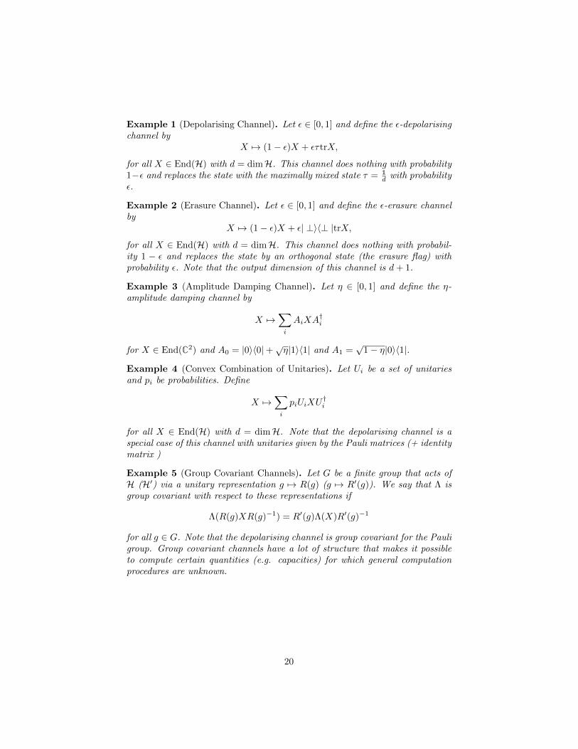
Example 1 (Depolarising Channel). Let ε ∈ [0, 1] and define the ε-depolarisingchannel by

X 7→ (1− ε)X + ετtrX,

for all X ∈ End(H) with d = dimH. This channel does nothing with probability1−ε and replaces the state with the maximally mixed state τ = 1

d with probabilityε.

Example 2 (Erasure Channel). Let ε ∈ [0, 1] and define the ε-erasure channelby

X 7→ (1− ε)X + ε| ⊥〉〈⊥ |trX,

for all X ∈ End(H) with d = dimH. This channel does nothing with probabil-ity 1 − ε and replaces the state by an orthogonal state (the erasure flag) withprobability ε. Note that the output dimension of this channel is d+ 1.

Example 3 (Amplitude Damping Channel). Let η ∈ [0, 1] and define the η-amplitude damping channel by

X 7→∑i

AiXA†i

for X ∈ End(C2) and A0 = |0〉〈0|+√η|1〉〈1| and A1 =√

1− η|0〉〈1|.

Example 4 (Convex Combination of Unitaries). Let Ui be a set of unitariesand pi be probabilities. Define

X 7→∑i

piUiXU†i

for all X ∈ End(H) with d = dimH. Note that the depolarising channel is aspecial case of this channel with unitaries given by the Pauli matrices (+ identitymatrix )

Example 5 (Group Covariant Channels). Let G be a finite group that acts ofH (H′) via a unitary representation g 7→ R(g) (g 7→ R′(g)). We say that Λ isgroup covariant with respect to these representations if

Λ(R(g)XR(g)−1) = R′(g)Λ(X)R′(g)−1

for all g ∈ G. Note that the depolarising channel is group covariant for the Pauligroup. Group covariant channels have a lot of structure that makes it possibleto compute certain quantities (e.g. capacities) for which general computationprocedures are unknown.

20

8 Lecture 7: Measurements

Corollary 13 (Instrument). Let Λ ∈⊕

i Hom(End(HA),End(HB)) be an in-strument. Then there are operators Kij ∈ Hom(HA,HB) s.th.

Λ(X) =∑i

|i〉〈i| ⊗KijXK†ij .

When the focus is not on the post-measurement state but only on the out-come probabilities, the following statement is important

Corollary 14 (POVM). Let Λ ∈⊕

i Hom(End(HA),C) be a measurement(without post-measurement state). Then there are positive semi-definite opera-tors Ei ∈ End(HA) s.th.

Λ(X) =∑i

|i〉〈i|trEiX.

and∑iEi = 1A. The set {Ei} are called a positive operator valued measure

(POVM) and its elements Ei the POVM elements.

Proof. By the previous corollary, we have

Λ(X) =∑i

|i〉〈i|trKijXK†ij .

Using the cyclicity of the trace, we obtain the result when defining Ei :=∑j K†ijKij and noting that these operators are positive semi-definite, since each

term in the sum is positive-semidefinite.

Note that given the Kraus operator sum decomposition of a quantum channel{Ki}, it is easy to obtain a Stinespring dilation. Simply define U =

∑i |i〉⊗Ki.

Corollary 15 (Naimark). Let Ei ∈ End(HA) be a POVM. Then there areorthogonal projectors Pi ∈ End(HA ⊕HE) satisfying

∑i Pi = 1A ⊕ 1E and

Ei = PPiP,

where P is the orthogonal projection in HA ⊕ HE onto HA. The Pi form aprojection-valued measurement (PVM) or von Neumann measurement. Thisrepresentation of the POVM is called a Naimark extension.

Proof. Let us start by writing the POVM elements in terms of their (non-

unique) Kraus operators Ei =∑j K†ijKij . Recall the Stinespring dilation U =∑

i |i〉⊗|j〉⊗Kij which is an isometry. Let us extend it to a unitary V = U⊕U⊥.This allows us to define a projective measurement with operators

Pi := V †|i〉〈i| ⊗ 1⊗ 1V

21

It now follows

trPPiPρ = trPi(ρ⊕ 0)

= trV †|i〉〈i| ⊗ 1⊗ 1V (ρ⊕ 0)

= tr|i〉〈i| ⊗ 1⊗ 1V (ρ⊕ 0)V †

= tr|i〉〈i| ⊗ 1⊗ 1UρU†

=∑j

KijρK†ij = trEiρ.

which concludes the proof.

Example 6 (Classical channels). Let P (y|x) be a classical channel given bya conditional probability distribution. We define the corresponding quantumchannel by

X 7→∑x,y

(tr|x〉〈x|X)P (y|x)|y〉〈y|.

Example 7 (Entanglement breaking channels). Let Ei be a POVM, and ρi bea set of quantum states. Then

X 7→∑i

(trEiX)ρi

is an entanglement breaking channel. It has its name from the fact that it breaksall entanglement with a possible reference, i.e. any state Λ⊗id(σAA′) is separable(not entangled), that is, of the form

∑i piσi ⊗ σ′i for a probability distribution

pi and states σi, σ′i.

Example 8 (Co-positive). A channel is co-positive if T ◦ Λ is CP, where T isthe transpose superoperator. Co-positive channels are mainly studied, becauseit is easier to characterise as entanglement-breaking and because entanglement-breaking channels are co-positive.

22

9 Lecture 8: Teleportation

Assume that Alice wants to send a qubit to Bob, but they do not have a qubitidentity channel, but that they only share an ebit (a maximally entangled stateof two qubits) and the ability to send two bits of classical information from Aliceto Bob. Can they simulate the sending of the qubit? Yes, they can. In order tosee how, let us phrase the problem mathematically.

The ebit is denoted by

|ψ00〉AB :=1√2|00 + 11〉,

and the classical channel of two bits by

CCA→CB (X) :=

1∑i,j=0

|ij〉〈ij|tr|ij〉〈ij|X.

Then we are looking for an encoding EAA→CA and a decoding DCBB→B suchthat[(DCBB→B) ◦ (CCA→CB ⊗ idB) ◦ (EAA→CA ⊗ idB)

](XA ⊗ |ψ00〉〈ψ00|AB) = XB .

(3)

SinceidA→B(XA) = XB

this corresponds to the desired qubit identity channel simulation.In the following, we will now construct the encoder and decoder, which is

known as the quantum teleportation protocol, as the qubit on Alice’s side isdestroyed and appears later on Bob’s side. In order to do so, we define theso-called Bell states:

|ψij〉 = 1⊗ σij |ψ00〉

where σij = σixσjz are derived from the Pauli matrices. Note that the Bell states

form an orthonormal basis for two qubits as

|ψ01〉 =1√2|00− 11〉, |ψ10〉 =

1√2|01 + 10〉, |ψ11〉 =

1√2|01− 10〉.

Note further that {|ψij〉〈ψij |} form a POVM (actually a PVM) and the associ-ated CPTP map is our encoding map

EAA→CA(YAA) =∑ij

|ij〉〈ij|CAtr|ij〉〈ij|AAYAA.

The decoding map is a Pauli operation controlled on the classical bits

DCBB→B(ZCBB) =∑ij

σijB→B(trCB |ij〉〈ij|CB ⊗ 1B · ZCBB)(σij

B→B)†

23

10 Lecture 9: Superdense Coding and Distances

Superdense coding is the task of sending two classical bits, via a single qubitidentity channel with the help of one shared ebit, that is

1[q − q] + 1[q → q] ≥ 2[c→ c].

Here, we are looking for maps ECAA→A and DBB→CB such that

CCA→CB (XCA) = DBB→CB ◦ idA→B ◦ ECAA→A(XCA ⊗ |ψ00〉〈ψ00|AB) (4)

where it is important that A is two-dimensional, whereas CA is four dimensional.It is actually very easy to achieve this task, we simply encode by applying (σij)T

onto the A part of the ebit, therefore generating the full set of Bell states onAB. Decoding is done by measuring BB in the Bell basis. Formally

ECAA→A(YCA) := (σijA )T trCA (|ij〉〈ij|CA ⊗ 1A · ZCAA) (σijA )T†

DBB→CB (ZBB) :=∑ij

|ij〉〈ij|CB trBB |ψij〉〈ψij |BB · ZBB

Note that it suffices to verify (4) on states diagonal in |ij〉:

DBB→CB ◦ idA→B ◦ ECAA→A(|ij〉〈ij|CA ⊗ |ψ00〉〈ψ00|AB)

= DBB→CB ◦ idA→B

((σijA )T ⊗ 1B · |ψ

00〉〈ψ00|AB · (σijA )T† ⊗ 1B

)mirror

= DBB→CB ◦ idA→B

(1A ⊗ σijB · |ψ

00〉〈ψ00|AB · (1A ⊗ (σijB

)†)

= DBB→CB(|ψij〉〈ψij |BB

)= |ij〉〈ij|CB

Just as we had discussed classically in the case of data compression, weare often happy with tolerating a small error when coding and decoding withquantum data. In order to do so, we need to have a good understanding whatapproximation means in the quantum case (both for states and channels). Anatural way to quantify distance is to introduce metrics based on norms. Forthe Schatten norms we find the distances

Tα(ρ, σ) := ||ρ− σ||α.

But we need to be a little careful with the choice of the norm. They are equiva-lent up to dimension factors of course, but exactly these dimension factors canbe very large (recall that the n qubit Hilbert space has dimension 2n). Classi-cally, we had used the variational distance. Its natural quantum generalisationis the trace distance δ(ρ, σ) := 1

2T1(ρ, σ) = 12 ||ρ− σ||1. It is a generalisation in

two ways. First, it reduces to to the variational distance when inserting statesthat are diagonal in the computational basis (that is why we can use the samesymbol) and second, because it can be characterised in terms of the variationaldistance:

25

Lemma 16. δ(ρ, σ) = maxEPOVM δ(E(ρ), E(σ)), where wlog E is a two outcomeprojective measurement.

Proof.

2δ(E(ρ), E(σ)) =∑i

|trEi(ρ− σ)|

= trE(ρ− σ) + tr(1− E)(σ − ρ)

where E is the sum of the Ei s.th. trEi(ρ − σ) ≥ 0. The first term is upperbounded by the sum of the positive eigenvalues and the second term is upperbounded by the sum of the negative eigenvalues. This shows that the RHS isupper bounded by the LHS. Equality is achieved for E the projector onto thesupport of the positive part of ρ− σ.

This lemma can be interpreted in the following way. Assume you are giventwo states, either ρ or σ each with a priori probability 1

2 and you are askedto guess which one it is. In order to answer the question, you perform a two-outcome POVM E0 and E1, where for the first outcome you guess ρ and for thesecond one σ. For a given POVM, the success probability is given by

psuccess =1

2(trE0ρ+ trE1σ) =

1

2(1 + δ(E(ρ), E(σ))).

The lemma then implies that the maximal success probability is given by

pmaxsuccess =

1

2(1 + δ(ρ, σ)).

The lemma also implies that the the trace distance is monotone (non-increasing)by application of a CPTP map on both arguments

δ(ρ, σ) ≥ δ(Λ(ρ),Λ(σ))

with equality if Λ is conjugation by a unitary.What makes the trace distance undesirable in many applications is that it

does behave very well with respect to purifying systems and also when consid-ering tensor products. It is therefore often better to work with the fidelity

F (ρ, σ) := ||√ρ√σ||1 = tr

√√ρσ√ρ.

Note that the formula reduces to√〈ψ|σ|ψ〉 in the case of ρ being pure and that

it reduces further to |〈ψ|φ〉| in the case, where also σ is pure. Uhlman’s theoremshows that the fidelity can also be regarded as an overlap of vectors in the caseof mixed states:

Theorem 17 (Uhlmann).

F (ρ, σ) = max |〈ψ|φ〉AB |

where the maximisation is taken over all purifications |ψ〉AB of ρA and |φ〉ABof ρB.

26

Proof. Define |Φ〉 =∑k |k〉|k〉 and note that by the above argument

|ψ〉AB =√ρA ⊗ V |Φ〉

and|φ〉AB =

√σA ⊗W |Φ〉

Hence〈ψ|AB |φ〉AB = 〈Φ|AB

√ρA√σA ⊗ V †W |Φ〉AB

This equals

〈Φ|AB√ρA√σA(V †W )T ⊗ 1|Φ〉AB = tr|√ρA

√σA|X(V †W )T

where |√ρA√σA|X is the polar decomposition of

√ρA√σA. We now apply the

Cauchy-Schwartz inequality to |√ρA√σA| and |√ρA

√σA|X(V †W )T in order

to upper bound the RHS by ||√ρ√σ||1. Equality is obtained for (V †W )T =

X†.

Uhlmann’s theorem implies that the fidelity is non-decreasing under theapplication of a CPTP map: F (ρ, σ) ≤ F (Λ(ρ),Λ(σ)), as the application of theCPTP map may be seen as requiring more structure of the purifications overwhich we optimize in the theorem.

Since for pure states ρ = |r〉〈r| and σ = |s〉〈s|, we can easily verify that (justexpand both as matrices in the o.n. basis {|r〉, |r⊥〉})

δ(ρ, σ) =√

1− F (ρ, σ)2,

the purified distanceP (ρ, σ) :=

√1− F (ρ, σ)2

can be characterised in terms of the trace distance:

P (ρ, σ) = maxρAB ,σAB

δ(ρAB , σAB).

where the maximisation extends over purifications of ρA ≡ ρ and σA ≡ σ.

27

11 Lecture 10: Quantum Data Compression

We are now ready to discuss the quantum analog of data compression. Thefirst quantum analog of the information source above that comes to mind isone that emits pure quantum states |ψi〉 ∈ Ca with distribution p(i), which, incontrast to the distinguishable symbols x, may not be necessarily orthogonal(〈ψi|ψj〉 6= 0) and thus not perfectly distinguishable. The encoder and decoderare completely positive and trace preserving (CPTP) maps

E : End(Ca)→ End(Cc)

D : End(Cc)→ End(Cb)

producing an output ρi = D ◦ E(|ψ〉〈ψ|i) whose average trace distance is sup-posed to satisfy ∑

i

piP (|ψ〉〈ψ|i, ρi) ≤ ε, (5)

Schumacher considered this scenario and it is indeed possible to repeat theclassical analysis. Note, however, that in general there are different ensem-bles {pi, |ψ〉〈ψ|i} and {p′j , |ψ′〉〈ψ′|j} that have the same average state ρ =∑i pi|ψ〉〈ψ|i =

∑j p′j |ψ〉〈ψ|j . Schumacher’s asymptotic analysis showed that

the data compression rate only depended on that average state and not on theactual ensemble. It would therefore be desirable to have a description of thesource that is independent of a choice of the ensemble. This is achieved by con-sidering a purification |ψ〉AR of ρA ≡ ρ and demanding the existence of CPTPmaps as above with the property that

P (|ψ〉〈ψ|AR, ρAR) ≤ ε, (6)

where ρAR = D ◦ E ⊗ idR(|ψ〉〈ψ|AR). Note that (6) immediately implies (5),since for any ensemble {pi, |ψ〉〈ψ|i} with average ρ and purification |ψ〉AR thereis a unitary V such that |ψ′〉AR = 1⊗ V |ψ〉AR =

∑i

√pi|ψi〉A|i〉R. This means

that we can replace |ψ〉 by |ψ′〉 in (6). Since the fidelity is non-increasing undermeasurement, we obtain (5) by measuring R in the computational basis.

It thus suffices entirely to minimize the storage (i.e. log c) under the con-straint (6). That is, the communication cost is given by

Cε(ρ) := minE,D{log c : (6) holds }

The protocol for the ε = 0 case is easily adapted from the classical case. Weconsider the projector P onto the support of ρ and define encoding and decodingoperations

E(X) = PXP + |1〉〈1|tr(1− P )X

D(Y ) = Y ⊕ 0.

28

We can easily confirm that (6) holds and that c = rankρ. Conversely, if weknow that if we choose c < rankρ than our classical consideration carries overand we find that reliable compression is not possible. Hence

C0(ρ) = H0(ρ) := log rankρ.

Now imagine that we pretend that instead of ρ we have a state σ for which weapply the perfect scheme. If P (ρ, σ) ≤ ε, then there are purifications |ψ〉〈ψ|ARand |ψ′〉〈ψ′|AR s.th.

P (ρ, σ) = P (|ψ〉〈ψ|AR, |ψ′〉〈ψ′|AR).

By the monotonicity of the purified distance we find that this upper bounds

P (D ◦ E ⊗ idR(|ψ〉〈ψ|AR),D ◦ E ⊗ idR(|ψ′〉〈ψ′|AR)) = P (ρAR, |ψ′〉〈ψ′|AR)).

By the triangle inequality we thus have

P (ρAR, |ψ〉〈ψ|AR) ≤ P (ρAR, |ψ′〉〈ψ′|AR) + P (|ψ′〉〈ψ′|AR, |ψ〉〈ψ|AR) ≤ 2ε.

Hence, we find

Cε(ρ) ≤ Hε/20 (ρ),

where Hε0(ρ) := minσ∈Bε(ρ)H(σ) for Bε(ρ) := {σ ≥ 0, trσ ≤ 1 : P (ρ, σ) ≤

ε}. Conversely, if we have a coding scheme satisfying (6), then consider theStinespring dilation VA→AA′ of D and define σAA′ := V◦E(ρ). Since P (ρ, σ) ≤ ε,we find P (ρA ⊗ |0〉〈0|A′ , σAA′) ≤ ε. We note that rankσAA′ ≤ c and that thesame is true for σ′ := trA′ |0〉〈0|A′σAA′ . It is easy to verify that σ := σ′/trσ′

satisfies P (ρ, σ) ≤ 2ε. Thus

Theorem 18.Hε/20 (ρ) ≥ Cε(ρ) ≥ H2ε

0 (ρ)

Then we have the following lemma

Lemma 19.Hε

0(ρ) ≤ Hε0(specρ)

The other direction can also be shown, incurring possibly a small loss inepsilon. As a corollary we obtain a formula for the data compression rate ofmany independent and identical sources:

Corollary 20 (Schumacher).

R(ρ) := limε→0

limn→∞

1

nCε(ρ⊗n) = H(ρ)

where H(ρ) = −trρ log ρ = H(λ) is the von Neumann entropy of ρ for λ theeigenvalues of ρ.

29

12 Lecture 11: Quantum Entropy

Often it is not the entropy (classical or quantum) of a system that is relevantin an information-theoretic context, but the conditional entropy. What theconditional distribution in relation to distribution, is the conditional entropy inrelation to the entropy. Just as there were many Renyi entropies, there will beeven more conditional Renyi entropies. For simplicity we will focus on the vonNeumann entropy (i.e. Renyi parameter equals 1) and will encounter some ofthe others when needed on the fly.

Classically, the conditional Shannon entropy H(X|Y)P is the entropy ofsystem X when conditioned on system Y, averaged over Y.

H(X|Y)P :=∑y

PY(y)H(X )PX|Y(·|y).

When Y is quantum it is not clear what it means to condition on it (we couldmeasure the system, but which measurement should we choose?). In order tocircumvent this problem for a moment, consider the formula

H(X|Y)P = H(XY)P −H(Y)P

which is easily verified to be true. Here, H(Y)P is the entropy of the marginaldistribution on Y. Here, the quantum generalisation

H(A|B)ρ = H(AB)ρ −H(B)ρ

makes immediate sense and it turns out to play an important role in quantuminformation theory. Curiously, and in contrast to its classical counterpart whichis always non-negative, the quantum conditional entropy can be negative! Canyou find out for which state? It is our goal in the rest of this course to discoverthe information-theoretic meaning behind this fact, which was publicised sometime ago by English media as scientist knows less than nothing 1.

Apart from this fact, quantum entropy seems to behave just like classicalentropy. It satisfies the intuitive property of subadditivity

H(AB) ≤ H(A) +H(B)

as well as its stronger version (strong subadditivity)

H(ABC) +H(C) ≤ H(AC) +H(BC)

whose equivalent version (weak monotonicity)

H(AB) +H(BC) ≥ H(A) +H(C)

can be derived from it by applying strong subadditivity to a purification ofABC. Quantum entropy may well satisfy any linear inequality (up to the factthat the conditional entropy is negative)∑

i

ciH(Xi) ≤ 0

1The scientist is Andreas Winter

30

that holds true for classical systems (many classical ones are known, but noadditional quantum ones have been found). That it suffices to study linearinequalities follows from the observation that the (closure of the) set of entropyvectors forms a cone.

Let us quickly prove the subadditivity property.

Lemma 21.H0(ρAB) ≤ H0(ρA) +H0(ρB)

Proof. Note that

H0(ρ) = min{log rkP : P 2 = P, PρP = ρ}

Then the RHS equals

min{log rkPA ⊗ PB : P 2A = PA, PAρAPA = ρA, P

2A = PA, PAρAPA = ρA}.

The condition implies PA ⊗PBρABPA ⊗PB = (PA ⊗ 1B) · (1A ⊗PB)ρAB(PA ⊗1B) · (1A ⊗ PB) = ρAB . Hence, the last expression is lower bounded by theLHS.

Lemma 22.H2ε

0 (ρAB) ≤ Hε0(ρA) +Hε

0(ρB)

Proof. Let PA (PB) be the projector onto the support of σA (σB), states weoptimise over in the RHS. Note that

P (ρA, σA) ≥ P (trPAρA, trPAσA) =√

1− (trPAρA)2,

since trPA· is a trace non-increasing CP map for which the purified distance ismonotone and since trPAσA = 1. The same holds for B. We also have

P (ρA, PAρAPA) =

√1− (tr

√√ρAPAρAPA

√ρA)2

=

√1− (tr

√(√ρAPA

√ρA)2)2

=√

1− (trPAρA)2,

and likewise for B. We now want to bound P (PA⊗PBρABPA⊗PB , ρAB) fromabove. For this, we note that

trPA ⊗ PBρAB ≥ trPAρA + trPBρB − 1,

which follows from the following small calculation

1 = tr(PA + (1A − PA))⊗ (PB + (1B − PB))ρAB

= trPA ⊗ PBρAB + trPA ⊗ (1B − PB)ρAB + tr(1A − PA)⊗ 1BρAB≤ trPA ⊗ PBρAB + tr(1B − PB)ρB + tr(1A − PA)ρA

= trPA ⊗ PBρAB + 1− trPBρB + 1− trPAρA

31

We now have

P (PA ⊗ PBρABPA ⊗ PB , ρAB) =√

1− (trPA ⊗ PBρAB)2

=√

(1− trPA ⊗ PBρAB)(1 + trPA ⊗ PBρAB)

≤√

2√

1− trPA ⊗ PBρAB≤√

2√

2− trPAρA − trPBρB

≤√

2√

1− (trPAρA)2 + 1− (trPBρB)2

≤√

2√P (PAρAPA, ρA)2 + P (PBρBPB , ρB)2

≤ 2ε

Thus we have constructed a subnormalised state

σAB := PA ⊗ PBρABPA ⊗ PB

with distance at most 2ε from ρAB from every σA and σB that were each ε-closeto ρA and ρB , respectively. Importantly, rkσAB ≤ rkσArkσB . This concludesthe proof after inspection of the definition of Hε

0.

Subadditivity now follows from Lemma 22 and the asymptotic equipartitionproperty

limε→0

limn→∞

1

nHε

0(ρ⊗n) = H(ρ)

which we have discussed previously.A proof of strong subadditivity can be given along the same lines but is

considerably more involved. Many other proofs of SSA exist, using matrixanalysis, operator convexity, representation theory (my own one), interpolationtheory, ..., highlighting its importance in the field: it is used in almost everytheorem proved in quantum information theory.

Just like the conditional entropy, one may define further derived quantitiessuch as the mutual information

I(A : B) := H(A)−H(A|B) = H(A) +H(B)−H(AB)

which is non-negative due to subadditivity and the conditional mutual informa-tion

I(A : B|C) := H(A|C)−H(A|BC)

= H(A|C) +H(B|C)−H(AB|C)

= H(AC) +H(BC)−H(C)−H(ABC)

which is non-negative due to strong subadditivity. They can be nicely repre-sented in the following Venn diagram.

Conditional entropy and conditional mutual information obey the followingchain rule, which is easily verified by expanding both sides in terms of theirelementary entropies:

H(AA′|C) = H(A|C) +H(A′|AC)

32

H(A) H(B)

H(C)

H(A|B) I(A:B|C)

Figure 1: Entropies of a three party system

I(A : BB′|C) = I(A : B|C) + I(A : B′|BC)

An important consequence of strong subadditivity is the data processinginequality

I(A : B′) ≤ I(A : B)

which holds for any CPTP map Λ : B → B′. It can be proved by representingΛ in its Stinespring form

Λ = trE ◦ UB→B′Eand by noting that I(A : B) = I(A : B′E) since local isometric evolution doesnot change global nor local eigenvalues and hence leaves the entropy invari-ant. Next, we expand I(A : B′E) = I(A : B′) + I(A : E|B′) and note thatI(A : E|B′) ≥ 0 due to SSA. This concludes the proof of the data processinginequality.

Since the eigenvalues are a continuous function of the density matrix, the vonNeumann entropy is as well. Such an abstract argument is often not enough,since continuity statements can involve large dimension factors. An importantresult is therefore Fannes inequality (here in the form by Winter following Au-denaert and Fannes and Alicki)

Theorem 23. Let ε ≥ δ(ρ, σ), then

|H(A|B)ρ −H(A|B)σ| ≤ 2ε log |A|+ (1 + ε)h(ε

1 + ε),

where h(x) = −x log x− (1− x) log(1− x) is the binary entropy function.

The proof is an exercise on this week’s sheet.

33

13 Lecture 12: The Decoupling Theorem

Let ρAR be a quantum state. It will be our goal to identity a large subsystem ofA that is decoupled from R. Whereas at first sight, decoupling sounds like theopposite of what quantum information theory is about (namely about generat-ing correlations), quantum systems have the curious property that correlationcannot be destroyed. This means if we are able to decouple in a controlledfashion, we will also be able to concentrate correlation in a controlled fashion.

Mathematically, for a state ρAR and a given unitary U : A → A1A2 we saythat A1 is ε-decoupled from R if

δ(ρA1R, τA1 ⊗ ρR) ≤ ε.

Note that this definition implicitly requires the decoupled system to be close tomaximally mixed. This aspect can be relaxed (ask Christian for more details).The following theorem gives a bound on A1:

Theorem 24 (Decoupling theorem). For a state ρAR choose

log |A2| ≥1

2(log |A| −H2(A|R)) +O(log

1

ε),

or equivalently

log |A1| ≤1

2(log |A|+H2(A|R)) +O(log

1

ε),

then there is a unitary U : A → A1A2 such that A1 is ε-decoupled from R.

Here, H2(A|R) := − log trρARρA|R, where ρA|R := 1A ⊗ ρ−1/2R ρAR1A ⊗ ρ−1/2

R ,is the conditional quantum Renyi entropy of order 2 (aka conditional quantumcollision entropy).

Corollary 25. For a state ρAR choose

log |A2| ≥1

2(Hε

0(A)−Hε2(A|R)) +O(log

1

ε),

then there is a unitary U : A → A1A2 such that A1 is 2ε-decoupled from R.Here, Hε

2(A|R)ρ := maxσ:P (ρ,σ)≤εHε2(A|R)σ.

Proof. Consider optimal σA and σ′AR and let P be the projector onto the supportof σ′A. Then

P (PσAP, ρA) ≤ P (PσAP, σ′A) + P (σ′A, ρA)

= P (PσAP, Pσ′AP ) + P (σ′A, ρA)

≤ P (σA, σ′A) + P (σ′A, ρA)

≤ 2ε

34

Lemma 26.||S||1 ≤

√trξ||ξ−1/4Sξ−1/4||2

Proof.

||S||1 = ||ξ 14 ξ−

14Sξ−

14 ξ

14 ||1

= tr|ξ 14 ξ−

14Sξ−

14 ξ

14 |

≤ trξ14 |ξ− 1

4Sξ−14 |ξ 1

4

= trξ12 |ξ− 1

4Sξ−14 |

≤√

trξ

√tr|ξ− 1

4Sξ−14 |2

=√

trξ

√tr(ξ−

14Sξ−

14 )2 =

√trξ||ξ−1/4Sξ−1/4||2

where the first inequality is seen by decomposing Hermitian ξ−14Sξ−

14 in its

spectral decomposition and the second is the Cauchy-Schwartz inequality.

Proof of Decoupling Theorem. According to Lemma 26 it suffices to show thatthere is a U s.th.

||ρA1R(U)− τA1⊗ ρR||22 ≤

ε2

|A1|

where ρA1R := (1A1⊗ ρR)−1/4ρA1R(1A1

⊗ ρR)−1/4. Note that it is sufficientto show that this is true on average (with some probability measure) over U ,since then we know that there exists one (such a proof technique is known as the“probabilistic method”. Since the unitary group is compact it is endowed with aprobability measure dU which is invariant under the group action, analogouslyto the uniform measure on a finite group. This measure is known as Haarmeasure and it is unique up to normalisation which we will choose as

∫dU = 1.

By the invariance of dU , the operator∫dUU ⊗ UX(U ⊗ U)†

commutes with U⊗U (actually this is all we require from the probability measuredU , a property known as a unitary 2-design property). One can verify byconcrete computation that an invariant operator must be a linear combinationof the identity matrix and the SWAP operator

SWAP =∑ij

|j〉〈i| ⊗ |i〉〈j|.

This fact can also be proved by use of elementary representation theory of theunitary group. In conclusion we find that∫

dUU ⊗ UX(U ⊗ U)† = α1 + βSWAP

35

holds for some α and β linear functions of X.Conceptually, we may interpret the following computation as the computa-

tion of a variance of ρA1R(U), when interpreted as a random variable Z. Westart by finding well-known relation E(Z −E(Z))2 = E(Z2)−E(Z)2.∫

dU ||ρA1R(U)− τA1⊗ ρR||22 =

∫dUtr(ρA1R(U)− τA1

⊗ ρR)2

=

∫dUtrρA1R(U)2 − tr(τA1

⊗ ρR)2

since∫dUρA1R(U) = τA1 ⊗ ρR. The first term on the RHS equals∫

dUtr((ρA1R(U)⊗ ρA1R(U))SWAPA1R)

since trγ2 = trγ ⊗ γSWAP. It equals

tr

(∫dUUA ⊗ UA(1⊗2

A2⊗ SWAPA1

)(U ⊗ U)†)⊗ SWAPRρA1R ⊗ ρA1R,

because SWAPAR = SWAPA ⊗ SWAPR. We now focus on the big bracket andset it equal to

α1A + βSWAPA.

Taking the trace of both sides of the equation, as well as the trace after havingmultiplied with SWAPA, we find the equations

tr1⊗2A2⊗ SWAPA1 = αtr1⊗2

A + βtrSWAPA

trSWAPA2 ⊗ 1⊗2A1

= αtrSWAPA + βtr1⊗2A

which are equivalent to

|A2|2|A1| = α|A|2 + β|A|

|A2||A1|2 = α|A|+ β|A|2

since trSWAPA = |A|. Solving the equations we find

α =|A2|2|A1| − |A1||A1|2|A2|2 − 1

≤ 1

|A1|

and by symmetry β ≤ 1|A2| . Hence∫

dU ||ρA1R(U)− τA1⊗ ρR||22 = αtr1⊗2

A ⊗ SWAPRρ⊗2AR + βtrSWAPARρ

⊗2AR −

1

|A1|trρ2

R

= αtrρ2R + βtrρ2

AR −1

|A1|trρ2

R

≤ 1

|A1|trρ2

R +1

|A2|trρ2

AR −1

|A1|trρ2

R

= 2− log |A2|−H2(A|R).

By choice of |A2|, the RHS is smaller than ε2/|A1|, which is what we set out toprove.

36

14 Lecture 13: Quantum State Merging: Part I

We are now prepared to state the task of quantum state merging. Considerthree players, Alice, Bob and a referee, jointly holding their respective shares ofa pure quantum state ρABR. We define the Cε(ρAB) as the minimal number ofqubits (the log of the dimension of the system) that Alice needs to send to Bobin a protocol resulting in Bob holding systems AB in ρABR satisfying

P (ρABR, ρABR) ≤ ε,

where ρABR is a purification of ρAB .Note that the problem reduces to quantum data transmission in the case of

Bob holding a trivial system. You may thus view it as quantum data transmis-sion where the receiver already has some information about the information tobe sent. In that sense, quantum state merging may be regarded as a quantumversion of the classical Slepian-Wolf coding: Here Alice and Bob are presentedwith an i.i.d. sequence of correlated random variables X and Y . The rate ofinformation that Alice needs to send to Bob such that he can recover X withhelp of his side information Y is given by H(X|Y ), the conditional Shannonentropy H(X|Y ) =

∑y p(y)H(X|Y = y).

Quantum state merging is a fundamental task in quantum information the-ory which, as we will see, has the distillation of entanglement between Alice andBob as a surprising byproduct.

Theorem 27 (One-shot State Merging).

C2√ε(ρAB) ≤ 1

2(Hε

0(A)−Hε2(A|R)) +O(log

1

ε).

When the state is a tensor product and we consider the rate per state

R(ρAB) := limε→0

limn→∞

1

nCε(ρ⊗nAB),

this bound becomes tight and we obtain

Theorem 28 (State Merging).

R(ρAB) =1

2I(A : R) =

1

2(H(A)−H(A|R)).

We will need the following small lemma.

Lemma 29.δ(ρ, σ) ≤ P (ρ, σ) ≤

√2δ(ρ, σ)

We had discussed the first inequality earlier. For a proof of the secondinequality see e.g. Nielsen and Chuang.

Proof of one-shot-state merging. Consider the following protocol:

37

• With the claimed choice of A1 Alice applies the unitary U : A → A1A2

from the decoupling theorem and finds that ρA1R is 2ε decoupled.

• She then sends A2 to Bob.

• Since Bob now has A2B and the total state is pure, he has a purificationρA1A2BR of ρA1R. Note that |φ〉〈φ|A1B1⊗ρABR is a purification of τA1⊗ρR.

• Since P (ρA1R, τA1⊗ρR)

lemma≤√

2√δ(ρA1R, τA1

⊗ ρR) ≤√

2 · 2ε, by Uhlmann’stheorem, there is a unitary VA2B→ABRB1

on Bob’s side such that the finalstate of the protocol

ρA1B1ABR := idA1R ⊗ VA2B→ABB1(ρA1A2BR)

has 2√ε distance to |φ〉〈φ|A1B1

⊗ ρABR.

Just looking at ABR we see that merging is complete with the claimed numberof qubits sent.

Note that Alice and Bob have distilled a maximally entangled state of12 (Hε

0(A) + Hε2(A|R)) + O(log 1

ε ) ebits as a byproduct. Nice. If we allow freeclassical communication, we can trade ebits and quantum communication andthus obtain a total ebit generation rate of Hε

2(A|R)O(log 1ε ) (if this number is

negative, then ebits are being consumed). We will come back to this a littlelater.

38

15 Lecture 14: State Merging Part II

Proof of State Merging. ≤: Inserting the one-shot state merging result into thedefinition of R we find

R(ρAB) = limε→0

limn→∞

1

nC2√ε(ρ⊗nAB),

≤ 1

2limε→0

limn→∞

1

nHε

0(A)− limε→0

limn→∞

1

nHε

2(A|R)

By the asymptotic equipartition theorem that we had seen before, the firstterm equals the von Neumann entropy of A. Similarly, one can shot that thesecond term equals H(A|R). The argument is here somewhat more complicatedand inspiration can be taken from our proof of subadditivity of von Neumannentropy. We omit it here, since we feel that there are no new conceptual stepspresent in the proof.≥: We begin by measuring the mutual information per copy present between

Bob and R at the start and at the end of the protocol. At the start, it is equalto I(B : R) and at the end it equals I(AB : R) (up to an error that vanishes asn→∞ (even for finite ε) due to Fannes inequality.

Observe that for every qubit Q sent from Alice to Bob, his mutual informa-tion with R can increase by at most 2:

I(BQ : R) = I(B : R) + I(Q : R|B) ≤ I(B : R) + 2,

where I(Q : R|B) = H(Q|R)−H(Q|BR) is the conditional mutual information.Since the final mutual information is I(AB : R), we find

I(AB : R) ≤ I(B : R) + 2R(ρAB)

Thus R(ρAB) ≥ 12 (I(AB : R) − I(B : R)) = 1

2 (I(A : R) + I(B : R|A) − I(B :R)) = 1

2I(A : R) since the total state is pure.

In the i.i.d. limit, the rate of ebits generated is

E(ρAB) =1

2(H(A) +H(A|R)).

In the presence of free classical communication, the total number of ebits be-comes

E(ρAB)−R(ρAB) = H(A|R) = −H(A|B),

where we used the fact that ABR is pure in the last step. This is the famoushashing bound by Devetak-Winter on the amount of entanglement that one candistill from ρAB

E→D (ρAB) ≥ E(ρAB)−R(ρAB) = H(A|R) = −H(A|B).

Remarkably, this number of ebits (if positive) is basically optimal even if wedisregard the constraint that the state should be merged properly.

39

Quantum Information Theory - Block 2 - 2015 - ku · PDF fileQuantum Information Theory - Block...

Documents

Transcript of Quantum Information Theory - Block 2 - 2015 - ku · PDF fileQuantum Information Theory - Block...