Quantum Hypothesis Testing and Non-Equilibrium Statistical ... · Quantum Hypothesis Testing and...

Quantum Hypothesis Testingand

Non-Equilibrium Statistical Mechanics

V. Jakšic1, Y. Ogata2, C.-A. Pillet3, R. Seiringer1

1Department of Mathematics and StatisticsMcGill University

805 Sherbrooke Street WestMontreal, QC, H3A 2K6, Canada

2Department of Mathematical SciencesUniversity of Tokyo

Komaba, Tokyo, 153-8914, Japan

3Centre de Physique Théorique – FRUMAMCNRS – Universités de Provence, de la Méditerrané et du Sud Toulon-Var

B.P. 20132, 83957 La Garde, France

Abstract. We extend the mathematical theory of quantum hypothesis testing to the general W ∗-algebraic settingand explore its relation with recent developments in non-equilibrium quantum statistical mechanics. In particular,we relate the large deviation principle for the full counting statistics of entropy flow to quantum hypothesis testingof the arrow of time.

2

Contents

1 Introduction 3

2 Prologue 5

2.1 Fenchel-Legendre transform . . . . . . . . . . . . . . . . . . . . . . . . . . . . . . . . . . . . . 5

2.2 Large deviation bounds . . . . . . . . . . . . . . . . . . . . . . . . . . . . . . . . . . . . . . . . 6

3 Approximately finite quantum hypothesis testing 9

3.1 Setup . . . . . . . . . . . . . . . . . . . . . . . . . . . . . . . . . . . . . . . . . . . . . . . . . 9

3.2 Bounds . . . . . . . . . . . . . . . . . . . . . . . . . . . . . . . . . . . . . . . . . . . . . . . . 11

3.3 Asymptotic hypothesis testing . . . . . . . . . . . . . . . . . . . . . . . . . . . . . . . . . . . . 12

3.4 Examples . . . . . . . . . . . . . . . . . . . . . . . . . . . . . . . . . . . . . . . . . . . . . . . 15

3.4.1 Quantum i.i.d. states . . . . . . . . . . . . . . . . . . . . . . . . . . . . . . . . . . . . . 15

3.4.2 Quantum spin systems . . . . . . . . . . . . . . . . . . . . . . . . . . . . . . . . . . . . 15

3.4.3 Quasi-free CAR states . . . . . . . . . . . . . . . . . . . . . . . . . . . . . . . . . . . . 17

4 Entropy production and full counting statistics 18

4.1 Setup . . . . . . . . . . . . . . . . . . . . . . . . . . . . . . . . . . . . . . . . . . . . . . . . . 18

4.2 Open systems . . . . . . . . . . . . . . . . . . . . . . . . . . . . . . . . . . . . . . . . . . . . . 20

4.3 Thermodynamic limit . . . . . . . . . . . . . . . . . . . . . . . . . . . . . . . . . . . . . . . . . 22

4.4 Large time limit . . . . . . . . . . . . . . . . . . . . . . . . . . . . . . . . . . . . . . . . . . . . 24

4.5 Testing the arrow of time . . . . . . . . . . . . . . . . . . . . . . . . . . . . . . . . . . . . . . . 26

5 Algebraic preliminaries 27

5.1 Notation . . . . . . . . . . . . . . . . . . . . . . . . . . . . . . . . . . . . . . . . . . . . . . . . 27

5.2 Modular structure . . . . . . . . . . . . . . . . . . . . . . . . . . . . . . . . . . . . . . . . . . . 28

5.3 Relative entropies . . . . . . . . . . . . . . . . . . . . . . . . . . . . . . . . . . . . . . . . . . . 29

5.4 Classical systems . . . . . . . . . . . . . . . . . . . . . . . . . . . . . . . . . . . . . . . . . . . 33

5.5 Finite systems . . . . . . . . . . . . . . . . . . . . . . . . . . . . . . . . . . . . . . . . . . . . . 34

6 Hypothesis testing in W ∗-algebras 34

6.1 Preliminaries . . . . . . . . . . . . . . . . . . . . . . . . . . . . . . . . . . . . . . . . . . . . . 34

6.2 Error exponents . . . . . . . . . . . . . . . . . . . . . . . . . . . . . . . . . . . . . . . . . . . . 37

6.3 Chernoff bound . . . . . . . . . . . . . . . . . . . . . . . . . . . . . . . . . . . . . . . . . . . . 39

6.4 Hoeffding bound . . . . . . . . . . . . . . . . . . . . . . . . . . . . . . . . . . . . . . . . . . . 39

6.5 Stein’s Lemma . . . . . . . . . . . . . . . . . . . . . . . . . . . . . . . . . . . . . . . . . . . . 42

3

7 Entropy production and full counting statistics for W ∗-dynamical systems 43

7.1 Setup . . . . . . . . . . . . . . . . . . . . . . . . . . . . . . . . . . . . . . . . . . . . . . . . . 43

7.2 Entropy production observable . . . . . . . . . . . . . . . . . . . . . . . . . . . . . . . . . . . . 44

7.3 Full counting statistics . . . . . . . . . . . . . . . . . . . . . . . . . . . . . . . . . . . . . . . . 46

7.4 Hypothesis testing of the arrow of time . . . . . . . . . . . . . . . . . . . . . . . . . . . . . . . . 47

8 Examples 49

8.1 Spin-fermion model . . . . . . . . . . . . . . . . . . . . . . . . . . . . . . . . . . . . . . . . . . 49

8.2 Electronic black box model . . . . . . . . . . . . . . . . . . . . . . . . . . . . . . . . . . . . . . 51

8.3 The XY quantum spin chain . . . . . . . . . . . . . . . . . . . . . . . . . . . . . . . . . . . . . 54

4

1 Introduction

Starting with the works [JP1, Ru1, Pi], the mathematical theory of non-equilibrium quantum statistical mechanicshas developed rapidly in recent years [Ab, AF, AP, AJPP1, AJPP2, FMS, FMU, JKP, JOP1, JOP2, JOP3, JOP4,JP2, JP3, JP4, MMS1, MMS2, MO, Na, Og1, Og2, Ro, Ru2, Tas, TM1, TM2]. The current research efforts arecentered around the theory of entropic fluctuations (see [JOPP1, JOPP2]) and it is these developments that willconcern us here.

Since Shannon’s rediscovery of Gibbs-Boltzmann entropy there has been a close interplay between informationtheory and statistical mechanics. One of the deepest links is provided by the theory of large deviations [DZ, El].We refer the reader to [Me] for a beautiful and easily accessible account of this interplay. In this context, it wasnatural to try to interpret recent results in non-equilibrium statistical mechanics in terms of quantum informationtheory.

The link can be roughly summarized as follows1. Consider the large deviation principle for the full countingstatistics for the repeated quantum measurement of the energy/entropy flow over the time interval [0, t] [LL, Ro,JOPP1]. Let I(θ) be the rate function and e(s) its Legendre transform. Let e(s) be the Chernoff error exponent inthe quantum hypothesis testing of the arrow of time, i.e., of the family of states (ωt/2, ω−t/2)t>0, where ω±t/2is the state of our quantum system at the time ±t/2. Then e(s) = e(s). In this paper we prove this result andelaborate on the relation between quantum hypothesis testing and non-equilibrium statistical mechanics.

Hypothesis testing has a long tradition in theoretical and applied statistics [Pe, Ch, LR]. During the last decademany results of classical hypothesis testing have been extended to the quantum domain [ACM, ANS, BDK1,BDK2, BDK3, Ha1, Ha2, HMO1, HMO2, HMO3, Ka, Mo, MHO, NS1, NS2, OH, ON]. The culmination of theseefforts was the proof of a long standing conjecture regarding the quantum Chernoff bound [ACM, ANS]. Thefollowing trace inequality of [ACM, ANS] played a key role in the resolution of this conjecture.

Proposition 1.1 Let A > 0 and B > 0 be matrices on Cn. Then

12

(TrA+ TrB − Tr |A−B|) ≤ TrA1−sBs (1.1)

holds for any s ∈ [0, 1].

Proof. (Communicated by N. Ozawa, unpublished). For X self-adjoint, X± denotes its positive/negative part.Decomposing A−B = (A−B)+ − (A−B)− one gets

12

(TrA+ TrB − Tr |A−B|) = TrA− Tr (A−B)+,

and (1.1) is equivalent toTrA− TrBsA1−s ≤ Tr (A−B)+. (1.2)

Note that B + (A − B)+ ≥ B and B + (A − B)+ = A + (A − B)− ≥ A. Since, for s ∈ [0, 1], the functionx 7→ xs is operator monotone (i.e., X ≤ Y ⇒ Xs ≤ Y s for any positive matrices X , Y ), we can write

TrA− TrBsA1−s = Tr(As −Bs)A1−s ≤ Tr ((B + (A−B)+)s −Bs)A1−s

≤ Tr ((B + (A−B)+)s −Bs)(B + (A−B)+)1−s

= TrB + Tr (A−B)+ − TrBs(B + (A−B)+)1−s

≤ Tr (A−B)+.

2

1Needless to say, all the notions discussed in this paragraph will be defined later in the paper.

5

We have singled out this result for the following reason. W ∗-algebras and modular theory provide a natural generalmathematical framework for quantum hypothesis testing. For example, Inequality (1.2) can be formulated in W ∗-algebraic language as

12

(ω(1) + ν(1)− ‖ω − ν‖) ≤ (Ωω|∆sν|ωΩω) (1.3)

for 0 ≤ s ≤ 1, where ω and ν are faithful, normal, positive linear functionals on aW ∗ algebra M in standard form,Ωω is the vector representative of ω in the natural cone and ∆ν|ω is the relative modular operator. The extensionof quantum hypothesis testing to W ∗-algebras was hindered by the fact that the original proof [ACM, ANS] ofthe inequality (1.2) could not be extended/generalized to a proof of (1.3). Ozawa’s proof, however, can and theinequality (1.3) was recently proven in [Og3]. An alternative proof, which links (1.3) to Araki-Masuda theory ofnon-commutative Lp-spaces, is given in Section 6.1.

In Section 6 we extend the mathematical theory of quantum hypothesis testing to the W ∗-algebraic setting andprove the Chernoff bound, the Hoeffding bound, and Stein’s Lemma. We develop a model independent axiomaticapproach to quantum hypothesis testing which clarifies its mathematical structure and reduces the study of concretemodels to the verification of the proposed axioms. We emphasize that apart from Inequality (1.3), whose proofis technically involved and has no classical counterpart, the proofs follow essentially line by line the classicalarguments. The verification of the large deviation axioms that underline the proofs leads to a novel class ofanalytic problems in quantum statistical mechanics.

To make the paper and our main points accessible to a reader without prior knowledge of modular theory, wedescribe in Sections 3 and 4 quantum hypothesis testing, non-equilibrium quantum statistical mechanics, and theirrelation in the context of finite quantum systems. Typical examples the reader should keep in mind are a quantumspin system or a Fermi gas confined to a finite part Λ of some infinite lattice L. Needless to say, the thermodynamiclimit Λ→ L has to be taken before the large time limit t→∞. The reader not familiar with (or not interested in)the algebraic theory may directly proceed to Section 8 after reading Sections 3 and 4.

For reasons of space we have not attempted to prove quantum hypothesis testing results under the most generalconditions possible. In particular, we shall only discuss hypothesis testing of faithful states (this restriction isinconsequential as far as statistical mechanics is concerned). The extensions to non-faithful states follow typicallyby straightforward limiting arguments (see [Og3] for an example).

This work is of a review nature. Our goal is to point to a surprising link between two directions of research whichwere largely unaware of each other, in a hope that they both may benefit from this connection. We shall discusshere only the single parameter full counting statistics for entropy flow and its relation to binary hypothesis testing.The multi-parameter full counting statistics describing the energy flow between different parts of the system is awell understood object but its relation with quantum hypothesis testing is unclear and would presumably involvemultiple quantum state discrimination which is poorly understood at the moment (the proposal of [NS1] appearsunsuitable in this context).

We also point out that for obvious space reasons this paper is not a review of either quantum statistical mechanicsor quantum hypothesis testing, but of the link between the two of them. The reader who wishes to learn more aboutthese topics individually may consult [AJPP1, JOPP1, ANS].

The paper is organized as follows. In Section 2 we review the results of Large Deviation Theory that we will need.Since these results are not stated/proven in this form in the classical references [DZ, El], we provide proofs for thereader’s convenience. In Section 3 we review the existing results in quantum hypothesis testing of finite quantumsystems. The non-equilibrium statistical mechanics of finite quantum systems is described in Section 4. Its rela-tion with quantum hypothesis testing is discussed in Section 4.5. In Section 5 we review the results of modulartheory that we need and give a new proof of the key preliminary inequality needed to prove (1.3) (Proposition5.5). Sections 6 and 7 are devoted to quantum hypothesis testing and non-equilibrium statistical mechanics ofinfinitely extended quantum systems described by W ∗-algebras and W ∗-dynamical systems. Finally, in Section 8

6

we describe several physical models for which the existence of the large deviation functionals have been provenand to which the results described in this paper apply.

Acknowledgments. The research of V.J. and R.S. was partly supported by NSERC. The research of Y.O. wassupported by JSPS Grant-in-Aid for Young Scientists (B), Hayashi Memorial Foundation for Female Natural Sci-entists, Sumitomo Foundation, and Inoue Foundation. The research of C.-A.P. was partly supported by ANR(grant 09-BLAN-0098). A part of this paper was written during the stay of the authors at the University of Cergy-Pontoise. We wish to thank L. Bruneau, V. Georgescu and F. Germinet for making these visits possible and fortheir hospitality.

2 Prologue

2.1 Fenchel-Legendre transform

Let [a, b] be a finite closed interval in R and e : [a, b] → R a convex continuous function. Convexity implies thatfor every s ∈]a, b[ the limits

D±e(s) = limh↓0

e(s± h)− e(s)±h

exist and are finite. Moreover, D−e(s) ≤ D+e(s), D+e(s) ≤ D−e(t) for s < t, and D−e(s) = D+e(s) outsidea countable set in ]a, b[. D+e(a) and D−e(b) also exist, although they may not be finite. If e′(s) exists for alls ∈]a, b[, then the mean value theorem implies that e′(s) is continuous on ]a, b[ and that

lims↓a

e′(s) = D+e(a), lims↑b

e′(s) = D−e(b).

We set e(s) = ∞ for s 6∈ [a, b]. Then e(s) is a lower semi-continuous convex function on R. The subdifferentialof e(s), ∂e(s), is defined by

∂e(s) =

]−∞, D+e(a)] if s = a;

[D−e(s), D+e(s)] if s ∈]a, b[;

[D−e(b),∞[ if s = b;

∅ if s 6∈ [a, b].

The functionϕ(θ) = sup

s∈[a,b]

(θs− e(s)) = sups∈R

(θs− e(s)) (2.1)

is called the Fenchel-Legendre transform of e(s). ϕ(θ) is finite and convex (hence continuous) on R. Ob-viously, a ≥ 0 ⇒ ϕ(θ) is increasing, and b ≤ 0 ⇒ ϕ(θ) is decreasing. The subdifferential of ϕ(θ) is∂ϕ(θ) = [D−ϕ(θ), D+ϕ(θ)]. The basic properties of the pair (e, ϕ) are summarized in:

Theorem 2.1 (1) sθ ≤ e(s) + ϕ(θ).

(2) sθ = e(s) + ϕ(θ)⇔ θ ∈ ∂e(s).

(3) θ ∈ ∂e(s)⇔ s ∈ ∂ϕ(θ).

(4) e(s) = supθ∈R(sθ − ϕ(θ)).

7

(5) If 0 ∈]a, b[, then ϕ(θ) is decreasing on ] − ∞, D−e(0)], increasing on [D+e(0),∞[, ϕ(θ) = −e(0) forθ ∈ ∂e(0), and ϕ(θ) > −e(0) for θ 6∈ ∂e(0).

(6)

ϕ(θ) =

aθ − e(a) if θ ≤ D+e(a);bθ − e(b) if θ ≥ D−e(b).

The proofs of these results are simple and can be found in [El, JOPP1].

The functionϕ(θ) = sup

s∈[a,b]

(θ(s− b)− e(s)) = ϕ(θ)− bθ (2.2)

will also play an important role in the sequel. Its properties are easily deduced from the properties of ϕ(θ). Inparticular, ϕ is convex, continuous and decreasing. It is a one-to-one map from ]−∞, D−e(b)] to [−e(b),∞[. Wedenote by ϕ−1 the inverse map.

Suppose now that a = 0 and b = 1. For r ∈ R let

ψ(r) =

−ϕ(ϕ−1(r)) if r ≥ −e(1);−∞ otherwise.

(2.3)

Proposition 2.2 (1)

ψ(r) = − sups∈[0,1[

−sr − e(s)1− s

. (2.4)

(2) ψ(r) is concave, increasing, finite for r > −e(1), and ψ(−e(1)) = e(1)−D−e(1).

(3) ψ(r) is continuous on ]− e(1),∞[ and upper-semicontinuous on R.

The proof of this proposition is elementary and we will omit it.

2.2 Large deviation bounds

In this paper we shall make use of some results of Large Deviation Theory, and in particular of a suitable variantof the Gärtner-Ellis theorem [DZ, El]. In this subsection we describe and prove the results we will need.

Let I ⊂ R+ be an unbounded index set, (Mt,Ft, Pt)t∈I a family of measure spaces, and Xt : Mt → R a familyof measurable functions. We assume that the measures Pt are finite for all t. The functions

R 3 s 7→ et(s) = log∫Mt

esXtdPt,

are convex (by Hölder’s inequality) and take values in ]−∞,∞]. We need

Assumption (LD). For some weight function I 3 t 7→ wt > 0 such that limt→∞ wt =∞ the limit

e(s) = limt→∞

1wtet(s),

exists and is finite for s ∈ [a, b]. Moreover, the function [a, b] 3 s 7→ e(s) is continuous.

8

Until the end of this section we shall assume that (LD) holds and set e(s) = ∞ for s 6∈ [a, b]. The Legendre-Fenchel transform ϕ(θ) of e(s) is defined by (2.1).

Proposition 2.3 (1) Suppose that 0 ∈ [a, b[. Then

lim supt→∞

1wt

logPt(x ∈Mt |Xt(x) > θwt) ≤

−ϕ(θ) if θ ≥ D+e(0);e(0) if θ < D+e(0).

(2.5)

(2) Suppose that 0 ∈]a, b]. Then

lim supt→∞

1wt

logPt(x ∈Mt |Xt(x) < θwt) ≤

−ϕ(θ) if θ ≤ D−e(0);e(0) if θ > D−e(0).

(2.6)

Proof. We shall prove (1); (2) follows from (1) applied to−Xt. For any s ∈]0, b], the Chebyshev inequality yields

Pt(x ∈Mt |Xt(x) > θwt) = Pt(x ∈Mt | esXt(x) > esθwt) ≤ e−sθwt∫Mt

esXtdPt,

and hencelim supt→∞

1wt

logPt(x ∈Mt |Xt(x) > θwt) ≤ − sups∈[0,b]

(sθ − e(s)).

Since

sups∈[0,b]

(sθ − e(s)) =

ϕ(θ) if θ ≥ D+e(0);−e(0) if θ < D+e(0),

the statement follows. 2

Proposition 2.4 Suppose that 0 ∈]a, b[, e(0) ≤ 0, and that e(s) is differentiable at s = 0. Then for any δ > 0there is γ > 0 such that for t large enough

Pt(x ∈Mt | |w−1t Xt(x)− e′(0)| ≥ δ) ≤ e−γwt .

Proof. Since ϕ(e′(0)) = −e(0), Theorem 2.1 (5) implies that ϕ(θ) > ϕ(e′(0)) ≥ 0 for θ 6= e′(0). Proposition2.3 implies

lim supt→∞

1wt

logPt(x ∈Mt | |w−1t Xt(x)− e′(0)| ≥ δ) ≤ −minϕ(e′(0) + δ), ϕ(e′(0)− δ),

and the statement follows. 2

Proposition 2.5 Suppose that e(s) is differentiable on ]a, b[. Then for θ ∈]D+e(a), D−e(b)[,

lim inft→∞

1wt

logPt(x ∈Mt |Xt(x) > θwt) ≥ −ϕ(θ). (2.7)

Proof. Let θ ∈]D+e(a), D−e(b)[ be given and let α > θ and ε > 0 be such that θ < α−ε < α < α+ε < D−e(b).Let sα ∈]a, b[ be such that e′(sα) = α (so ϕ(α) = αsα − e(sα)). Let

dPt = e−et(sα)esαXtdPt.

9

Then Pt is a probability measure on (Mt,Ft) and

Pt(x ∈Mt |Xt(x) > θwt) ≥ Pt(x ∈Mt |w−1t Xt(x) ∈ [α− ε, α+ ε])

= eet(sα)

∫w−1

t Xt∈[α−ε,α+ε]e−sαXtdPt

≥ eet(sα)−sααwt−|sα|wtεPt(x ∈Mt |w−1t Xt ∈ [α− ε, α+ ε]).

(2.8)

Now, if et(s) = log∫Mt

esXtdPt, then et(s) = et(s+ sα)− et(sα) and so for s ∈ [a− sα, b− sα],

limt→∞

1wtet(s) = e(s+ sα)− e(sα).

Since e′(0) = e′(sα) = α, it follows from Proposition 2.4 that

limt→∞

1wt

log Pt(x ∈Mt |w−1t Xt(x) ∈ [α− ε, α+ ε]) = 0,

and (2.8) yields

lim inft→∞

1wt

logPt(x ∈Mt |Xt(x) > θwt) ≥ −sαα+ e(sα)− |sα|ε = −ϕ(α)− |sα|ε.

The statement follows by taking first ε ↓ 0 and then α ↓ θ. 2

The following local version of the Gärtner-Ellis theorem is a consequence of Propositions 2.3 and 2.5.

Theorem 2.6 If e(s) is differentiable on ]a, b[ and 0 ∈]a, b[ then, for any open set J ⊂]D+e(a), D−e(b)[,

limt→∞

1wt

logPt(x ∈Mt |w−1t Xt(x) ∈ J) = − inf

θ∈Jϕ(θ).

Proof. Lower bound. For any θ ∈ J and δ > 0 such that ]θ − δ, θ + δ[⊂ J one has

Pt(x ∈Mt |w−1t Xt(x) ∈ J) ≥ Pt(x ∈Mt |w−1

t Xt(x) ∈]θ − δ, θ + δ[),

and it follows from Proposition 2.5 that

lim inft→∞

1wt

logPt(x ∈Mt |w−1t Xt(x) ∈ J) ≥ −ϕ(θ − δ).

Letting δ ↓ 0 and optimizing over θ ∈ J, we obtain

lim inft→∞

1wt

logPt(x ∈Mt |w−1t Xt(x) ∈ J) ≥ − inf

θ∈Jϕ(θ). (2.9)

Upper bound. By Part (5) of Theorem 2.1, we have ϕ(θ) = −e(0) for θ = e′(0) and ϕ(θ) > −e(0) otherwise.Hence, if e′(0) ∈ J (the closure of J), then

lim supt→∞

1wt

logPt(x ∈Mt |w−1t Xt(x) ∈ J) ≤ e(0) = − inf

θ∈Jϕ(θ).

10

In the case e′(0) 6∈ J, there exist α, β ∈ J such that e′(0) ∈]α, β[⊂ R \ J. It follows that

Pt(x ∈Mt |w−1t Xt(x) ∈ J)

≤ Pt(x ∈Mt |w−1t Xt(x) < α) + Pt(x ∈Mt |w−1

t Xt(x) > β)≤ 2 max

(Pt(x ∈Mt |w−1

t Xt(x) < α), Pt(x ∈Mt |w−1t Xt(x) > β)

),

and Proposition 2.3 yields

lim supt→∞

1wt

logPt(x ∈Mt |w−1t Xt(x) ∈ J) ≤ −min(ϕ(α), ϕ(β)).

Finally, by Part (5) of Proposition 2.1, one has

infθ∈J

ϕ(θ) = min(ϕ(α), ϕ(β)),

and thereforelim supt→∞

1wt

logPt(x ∈Mt |w−1t Xt(x) ∈ J) ≤ − inf

θ∈Jϕ(θ) (2.10)

holds for any J ⊂]D+e(a), D−e(b)[. The result follows from the bounds (2.9) and (2.10). 2

3 Approximately finite quantum hypothesis testing

3.1 Setup

Consider a quantum system Q described by a finite dimensional Hilbert space H. We denote by OH (or Owhenever the meaning is clear within the context) the ∗-algebra of all linear operators on H, equipped with theusual operator norm. The symbol 1H (or simply 1) stands for the unit ofOH. The spectrum of A ∈ OH is denotedby sp(A). OH,self (or simply Oself ) is the set of all self-adjoint elements of OH. A ∈ OH,self is positive, writtenA ≥ 0, if sp(A) ⊂ [0,∞[. For A ∈ OH,self and λ ∈ sp(A), Pλ(A) denotes the spectral projection of A. We adoptthe shorthand notation

sA =∑

06=λ∈sp(A)

Pλ(A), A± = ±∑

λ∈sp(A),±λ>0

λPλ(A), |A| = A+ −A−.

sA is the orthogonal projection on the range of A and A± are the positive/negative parts of A.

A linear functional ν : O → C is called:

(1) hermitian if ν(A) ∈ R for all A ∈ Oself ;

(2) positive if ν(A∗A) ≥ 0 for all A ∈ O;

(3) a state if it is positive and normalized by ν(1) = 1;

(4) faithful if it is positive and such that ν(A∗A) = 0 implies A = 0 for any A ∈ O.

For any ν ∈ O, A 7→ Tr νA defines a linear functional on O, i.e., an element of the dual space O∗. Any linearfunctional on O arises in this way. In the following, we shall identify ν ∈ O with the corresponding linearfunctional and write ν(A) = Tr νA. With this identification, the norm of the dual space O∗ is just the trace normon O, i.e., ‖ν‖ = Tr |ν| = |ν|(1) with |ν| = (ν∗ν)1/2. A functional ν is hermitian iff ν ∈ Oself and positive iff

11

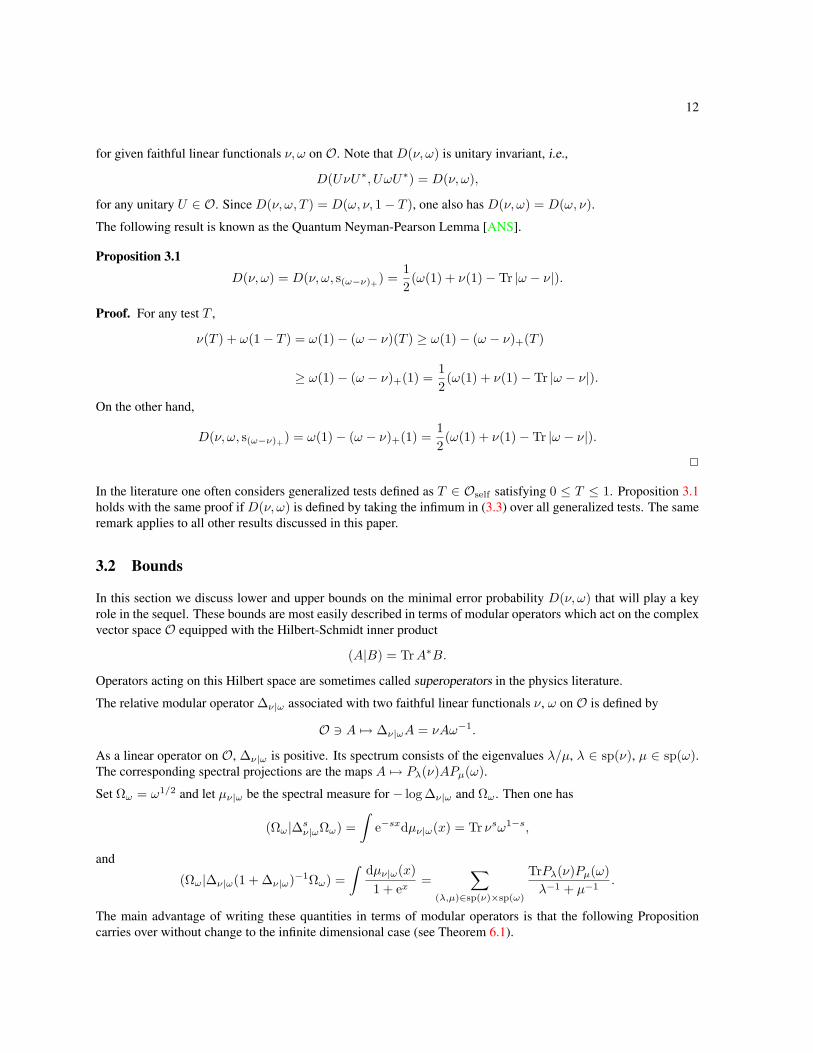
ν ≥ 0 as an operator. If ν ≥ 0 then it is faithful iff sp(ν) ⊂]0,∞[, which we denote by ν > 0. The functional νis a state iff the operator ν is a density matrix, i.e., ν ≥ 0 and ν(1) = Tr ν = 1. If ν is a positive linear functionalthen sν is its support projection, the smallest orthogonal projection P such that ν(1 − P ) = 0. In particular‖ν‖ = ν(1) = ν(sν) and ν is faithful iff sν = 1. If ν is a Hermitian linear functional then ν± are positive linearfunctionals such that sν+sν− = 0, ν = ν+ − ν− (the Jordan decomposition of ν) and ‖ν‖ = ν+(1) + ν−(1).

Let ν and ω be positive linear functionals. The relative entropy of ν w.r.t. ω is given by

Ent(ν|ω) =

Tr ν(logω − log ν), if sν ≤ sω,

−∞ otherwise.(3.1)

Rényi’s relative entropy of ν w.r.t. ω is the convex function

[0, 1] 3 s 7→ Ents(ν|ω) =

log Tr νsω1−s, if sνsω 6= 0,

−∞ otherwise,

which clearly satisfies Ents(ν|ω) = Ent1−s(ω|ν). If sν ≤ sω then this function has a real analytic extension tos ∈]0,∞[ and

dds

Ents(ν|ω)∣∣∣∣s=1

= −Ent(ν|ω). (3.2)

The observables of the quantum system Q are described by elements of Oself and its physical states are states onO, i.e., density matrices. The possible outcomes of a measurement of A are the eigenvalues a ∈ sp(A). If thesystem is in the state ν, then the probability to observe a is ν(Pa(A)). In particular, the expectation value of A isν(A).

The setup of quantum hypothesis testing is a direct generalization of the corresponding setup in classical statistics[LR]. Let ν 6= ω be two faithful2 states such that one of the following two competing hypotheses holds:

Hypothesis I : Q is in the state ω;

Hypothesis II : Q is in the state ν.

A test is a projection T ∈ Oself and the result of a measurement of the corresponding observable is either 0 or 1.The purpose of a test is to discriminate between the two hypotheses. Given the outcome of the measurement of Tone chooses Hypothesis I or II. More precisely, if the outcome is 1 one accepts I and rejects II. Otherwise, if theoutcome is 0, one accepts II and rejects I. To a given test T one can associate two kinds of errors. A type-I erroroccurs when the system is in the state ω but the outcome of the test is 0. The conditional probability of such anerror, given that the state of the system is ω, is ω(1− T ). If the system is in the state ν and the outcome of the testis 1, we get a type-II error, with conditional probability ν(T ).

Assuming that Bayesian probabilities can be assigned to the states ω and ν, i.e., that the state of the system is ωwith probability p ∈]0, 1[ and ν with probability 1− p, the total error probability is equal to

pω(1− T ) + (1− p) ν(T ),

which we wish to minimize over T . It is convenient to absorb the scalar factors into ν and ω and consider thequantities

D(ν, ω, T ) = ν(T ) + ω(1− T ),

D(ν, ω) = infTD(ν, ω, T ),

(3.3)

2In this paper, for simplicity of the exposition, we shall only consider faithful states. We note, however, that most results extend to thegeneral case by a straightforward limiting argument.

12

for given faithful linear functionals ν, ω on O. Note that D(ν, ω) is unitary invariant, i.e.,

D(UνU∗, UωU∗) = D(ν, ω),

for any unitary U ∈ O. Since D(ν, ω, T ) = D(ω, ν, 1− T ), one also has D(ν, ω) = D(ω, ν).

The following result is known as the Quantum Neyman-Pearson Lemma [ANS].

Proposition 3.1D(ν, ω) = D(ν, ω, s(ω−ν)+) =

12

(ω(1) + ν(1)− Tr |ω − ν|).

Proof. For any test T ,

ν(T ) + ω(1− T ) = ω(1)− (ω − ν)(T ) ≥ ω(1)− (ω − ν)+(T )

≥ ω(1)− (ω − ν)+(1) =12

(ω(1) + ν(1)− Tr |ω − ν|).

On the other hand,

D(ν, ω, s(ω−ν)+) = ω(1)− (ω − ν)+(1) =12

(ω(1) + ν(1)− Tr |ω − ν|).

2

In the literature one often considers generalized tests defined as T ∈ Oself satisfying 0 ≤ T ≤ 1. Proposition 3.1holds with the same proof if D(ν, ω) is defined by taking the infimum in (3.3) over all generalized tests. The sameremark applies to all other results discussed in this paper.

3.2 Bounds

In this section we discuss lower and upper bounds on the minimal error probability D(ν, ω) that will play a keyrole in the sequel. These bounds are most easily described in terms of modular operators which act on the complexvector space O equipped with the Hilbert-Schmidt inner product

(A|B) = TrA∗B.

Operators acting on this Hilbert space are sometimes called superoperators in the physics literature.

The relative modular operator ∆ν|ω associated with two faithful linear functionals ν, ω on O is defined by

O 3 A 7→ ∆ν|ωA = νAω−1.

As a linear operator on O, ∆ν|ω is positive. Its spectrum consists of the eigenvalues λ/µ, λ ∈ sp(ν), µ ∈ sp(ω).The corresponding spectral projections are the maps A 7→ Pλ(ν)APµ(ω).

Set Ωω = ω1/2 and let µν|ω be the spectral measure for − log ∆ν|ω and Ωω . Then one has

(Ωω|∆sν|ωΩω) =

∫e−sxdµν|ω(x) = Tr νsω1−s,

and

(Ωω|∆ν|ω(1 + ∆ν|ω)−1Ωω) =∫

dµν|ω(x)1 + ex

=∑

(λ,µ)∈sp(ν)×sp(ω)

TrPλ(ν)Pµ(ω)λ−1 + µ−1

.

The main advantage of writing these quantities in terms of modular operators is that the following Propositioncarries over without change to the infinite dimensional case (see Theorem 6.1).

13

Proposition 3.2 (1) Upper bound: for any s ∈ [0, 1],

D(ν, ω) ≤ (Ωω|∆sν|ωΩω).

(2) Lower bound:D(ν, ω) ≥ (Ωω|∆ν|ω(1 + ∆ν|ω)−1Ωω).

Proof. Part (1) follows from Proposition 1.1 and we only need to prove Part (2). For any test T , one has

ν(T ) =∑

λ∈sp(ν)

λTrTPλ(ν)T =∑


λµ−1ω(TPλ(ν)TPµ(ω)),

ω(1− T ) =∑


ω((1− T )Pλ(ν)(1− T )Pµ(ω)).

Since, for κ ≥ 0,

κTPλ(ν)T + (1−T )Pλ(ν)(1−T ) =κ

1 + κPλ(ν) +

11 + κ

(1− (1 +κ)T )Pλ(ν)(1− (1 +κ)T ) ≥ κ

1 + κPλ(ν),

we derive

ν(T ) + ω(1− T ) ≥∑


λ/µ

1 + λ/µω(Pλ(ν)Pµ(ω)) = (Ωω|∆ν|ω(1 + ∆ν|ω)−1Ωω).

2

3.3 Asymptotic hypothesis testing

After these preliminaries, we turn to asymptotic hypothesis testing. For each n ∈ N, let Qn be a quantum systemdescribed by the finite dimensional Hilbert spaces Hn and let (νn, ωn) be a pair of faithful linear functionals onOHn . Let wn > 0 be given weights such that limn→∞ wn =∞. Error exponents of the Chernoff type associatedto (νn, ωn, wn) are defined by

D = lim supn→∞

1wn

logD(νn, ωn),

D = lim infn→∞

1wn

logD(νn, ωn).

An immediate consequence of Proposition 3.2 (1) is:

Proposition 3.3D ≤ inf

s∈[0,1]lim supn→∞

1wn

Ents(νn|ωn).

Lower bounds in asymptotic hypothesis testing are intimately linked with the theory of large deviations and todiscuss them we need

Assumption (AF1). The limit

e(s) = limn→∞

1wn

Ents(νn|ωn)

exists and is finite for s ∈ [0, 1]. The function s 7→ e(s) is continuous on [0, 1], differentiable on ]0, 1[,and D+e(0) < D−e(1).

14

Note that the limiting function s 7→ e(s) is convex on [0, 1].

The following result is known as the Chernoff bound.

Theorem 3.4 Suppose that Assumption (AF1) holds. Then

D = D = infs∈[0,1]

e(s).

Proof. By Proposition 3.3, we only need to prove that

D ≥ infs∈[0,1]

e(s).

Applying Chebyshev’s inequality to Part (2) of Proposition 3.2 one easily shows that

D ≥ lim infn→∞

1wn

logµνn|ωn(]−∞,−θwn[), (3.4)

for any θ ≥ 0. Suppose first that e(0) ≤ e(1). Then D−e(1) > 0 and since

e(s) = limn→∞

1wn

log∫

e−sxdµνn|ωn(x),

Proposition 2.5 implies that for θ ∈]D+e(0), D−e(1)[,

lim infn→∞

1wn

logµνn|ωn(]−∞,−θwn[) ≥ −ϕ(θ), (3.5)

withϕ(θ) = sup

s∈[0,1]

(θs− e(s)).

If 0 > D+e(0) then 0 ∈]D+e(0), D−e(1)[ and it follows from (3.4) and (3.5) that

D ≥ −ϕ(0) = infs∈[0,1]

e(s).

If 0 ≤ D+e(0), then (3.4) and (3.5) imply that D ≥ −ϕ(θ) for any θ ∈]D+e(0), D−e(1)[ and since ϕ iscontinuous, one has

D ≥ −ϕ(D+e(0)) = e(0) ≥ infs∈[0,1]

e(s).

If e(0) > e(1), one derives the result by exchanging the roles of νn and ωn, using the fact that D(νn, ωn) =D(ωn, νn). 2

We now turn to asymmetric hypothesis testing. Until the end of this section we assume that νn and ωn are states.The asymmetric hypothesis testing concerns individual error probabilities ωn(1 − Tn) (type-I error) and ν(Tn)(type-II error). For r ∈ R, error exponents of the Hoeffding type are defined by

B(r) = infTn

lim supn→∞

1wn

logωn(1− Tn)∣∣∣∣ lim sup

n→∞

1wn

log νn(Tn) < −r,

B(r) = infTn

lim infn→∞

1wn


n→∞

1wn

log νn(Tn) < −r,

B(r) = infTn

limn→∞

1wn


n→∞

1wn

log νn(Tn) < −r,

15

where in the last case the infimum is taken over all families of tests Tn for which limn1wn

logωn(1−Tn) exists.These exponents give the best exponential convergence rate of type-I error under the exponential convergenceconstraint on the type-II error. An alternative interpretation is in terms of state concentration: as n → ∞ thestates ωn and νn are concentrating along orthogonal subspaces and the Hoeffding exponents quantify the degreeof this separation on the exponential scale. In classical statistics the Hoeffding exponents can be traced back to[Ho, CL, Bl].

The following result is known as the Hoeffding bound [Ha2, Na]:

Theorem 3.5 Suppose that Assumption (AF1) holds. Then for all r ∈ R,

B(r) = B(r) = B(r) = − sups∈[0,1[

−sr − e(s)1− s

.

For ε ∈]0, 1[, error exponents of the Stein type are defined by

Bε = infTn

lim supn→∞

1wn

logωn(1− Tn)∣∣∣∣ νn(Tn) ≤ ε

,

Bε = infTn

lim infn→∞

1wn


,

Bε = infTn

limn→∞

1wn


,

where in the last case the infimum is taken over all families of tests Tn for which limn1wn

logωn(1−Tn) exists.Note that if

βn(ε) = infT :νn(T )≤ε

ωn(1− T ),

thenlim infn→∞

1wn

log βn(ε) = Bε, lim supn→∞

1wn

log βn(ε) = Bε.

The study of Stein’s exponents in the quantum setting goes back to [HP]. To discuss these exponents we need

Assumption (AF2). For some δ > 0, the limit

e(s) = limn→∞

1wn

Ents(νn|ωn),

exists and is finite for all s ∈ [0, 1 + δ[. The function s 7→ e(s) is differentiable at s = 1.

Relation (3.2), Assumption (AF2) and convexity imply

e′(1) = − limn→∞

1wn

Ent(νn|ωn).

In accordance with the terminology used in non-equilibrium statistical mechanics, we shall call

Σ+ = e′(1)

the entropy production of the hypothesis testing. The following result is known as Stein’s Lemma [HP, ON].

16

Theorem 3.6 Suppose that Assumptions (AF1)–(AF2) hold. Then for all ε ∈]0, 1[,

Bε = Bε = Bε = −Σ+.

Remark. This result holds under more general conditions then (AF1) and (AF2), see Section 6.5.

Just like the Chernoff bound, the Hoeffding bound and Stein’s Lemma (Theorems 3.5 and 3.6) are easy conse-quences of Proposition 3.2 and the Gärtner-Ellis theorem. To avoid repetitions, we refer the reader to Sections 6.4and 6.5 for their proofs in the general W ∗-algebraic setting. As we have already mentioned, given Proposition 3.2(and its W ∗-algebraic generalization), the proofs follow line by line the classical arguments. The non-trivial as-pects of non-commutativity emerge only in the verification of Assumptions (AF1)–(AF2) in the context of concretequantum statistical models.

3.4 Examples

3.4.1 Quantum i.i.d. states

Quantum i.i.d. states are the simplest (and most widely studied) examples of quantum hypothesis testing. Asymp-totic hypothesis testing for such states can be interpreted in terms of multiple measurements on independent,statistically equivalent systems. LetK be a finite dimensional Hilbert space, ν and ω two faithful linear functionalson OK, and

Hn = ⊗nj=1K, νn = ⊗nj=1ν, ωn = ⊗nj=1ω.

For s ∈ R, one hasTr νsnω

1−sn = (Tr νsω1−s)n

and, taking the weights wn = n, we see that

e(s) = limn→∞

1n

Ents(νn|ωn) = Ents(ν|ω) =∑


λsµ1−sTrPλ(ν)Pµ(ω).

The function e(s) is real-analytic on R and is strictly convex iff ν 6= ω. In particular, Theorems 3.4, 3.5 and 3.6hold for quantum i.i.d. states.

3.4.2 Quantum spin systems

Let P be the collection of all finite subsets of Zd. For X ∈ P , |X| denotes the cardinality of X (the number ofelements of X), diamX = max|x − y| |x, y ∈ X is the diameter of X , and X + a = x + a |x ∈ X is thetranslate of X by a ∈ Zd.

Suppose that a single spin is described by the finite dimensional Hilbert space K. We attach a copy Kx of K toeach site x ∈ Zd. For X ∈ P we define HX = ⊗x∈XKx and OX = OHX . ‖A‖ is the usual operator norm ofA ∈ OX . For X ⊂ Y , the identity HY = HX ⊗HY \X yields a natural identification of OX with a ∗-subalgebraofOY . For a ∈ Zd, we denote by T a : Kx → Kx+a the identity map. T a extends to a unitary mapHX → HX+a.

An interaction is a collection Φ = ΦXX∈P such that ΦX ∈ OX,self and T aΦXT−a = ΦX+a for any a ∈ Zd.We set

|||Φ||| =∑X30

|X|−1‖ΦX‖, ‖Φ‖ =∑X30

‖ΦX‖.

The interaction Φ is finite range if for some R > 0 and any X ∈ P such that diamX > R, ΦX = 0.

17

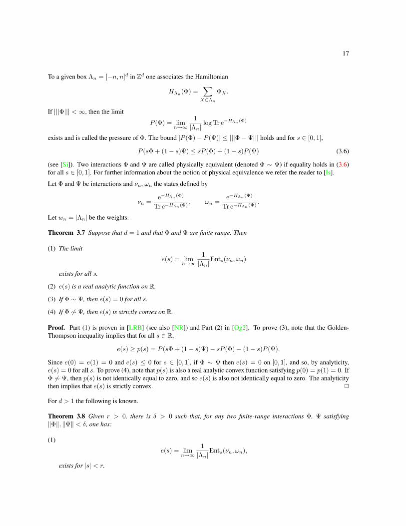
To a given box Λn = [−n, n]d in Zd one associates the Hamiltonian

HΛn(Φ) =∑X⊂Λn

ΦX .

If |||Φ||| <∞, then the limit

P (Φ) = limn→∞

1|Λn|

log Tr e−HΛn (Φ)

exists and is called the pressure of Φ. The bound |P (Φ)− P (Ψ)| ≤ |||Φ−Ψ||| holds and for s ∈ [0, 1],

P (sΦ + (1− s)Ψ) ≤ sP (Φ) + (1− s)P (Ψ) (3.6)

(see [Si]). Two interactions Φ and Ψ are called physically equivalent (denoted Φ ∼ Ψ) if equality holds in (3.6)for all s ∈ [0, 1]. For further information about the notion of physical equivalence we refer the reader to [Is].

Let Φ and Ψ be interactions and νn, ωn the states defined by

νn =e−HΛn (Φ)

Tr e−HΛn (Φ), ωn =

e−HΛn (Ψ)

Tr e−HΛn (Ψ).

Let wn = |Λn| be the weights.

Theorem 3.7 Suppose that d = 1 and that Φ and Ψ are finite range. Then

(1) The limit

e(s) = limn→∞

1|Λn|

Ents(νn, ωn)

exists for all s.

(2) e(s) is a real analytic function on R.

(3) If Φ ∼ Ψ, then e(s) = 0 for all s.

(4) If Φ 6∼ Ψ, then e(s) is strictly convex on R.

Proof. Part (1) is proven in [LRB] (see also [NR]) and Part (2) in [Og2]. To prove (3), note that the Golden-Thompson inequality implies that for all s ∈ R,

e(s) ≥ p(s) = P (sΦ + (1− s)Ψ)− sP (Φ)− (1− s)P (Ψ).

Since e(0) = e(1) = 0 and e(s) ≤ 0 for s ∈ [0, 1], if Φ ∼ Ψ then e(s) = 0 on [0, 1], and so, by analyticity,e(s) = 0 for all s. To prove (4), note that p(s) is also a real analytic convex function satisfying p(0) = p(1) = 0. IfΦ 6∼ Ψ, then p(s) is not identically equal to zero, and so e(s) is also not identically equal to zero. The analyticitythen implies that e(s) is strictly convex. 2

For d > 1 the following is known.

Theorem 3.8 Given r > 0, there is δ > 0 such that, for any two finite-range interactions Φ, Ψ satisfying‖Φ‖, ‖Ψ‖ < δ, one has:

(1)

e(s) = limn→∞

1|Λn|

Ents(νn, ωn),

exists for |s| < r.

18

(2) e(s) is real analytic on ]− r, r[.

(3) If Φ ∼ Ψ, then e(s) = 0 for s ∈]− r, r[.

(4) If Φ 6∼ Ψ, then e(s) is strictly convex ]− r, r[.

Remark 1. The existence of e(s) is established in [NR] (see also [LRB]). The real analyticity follows fromProposition 7.10 in [NR]. Parts (3) and (4) are proven in the same way as in Theorem 3.7.

Remark 2. One can get an explicit estimate on δ in terms of r by combining Theorem 6.2.4 in [BR2] andProposition 7.10 in [NR].

Remark 3. Theorem 3.8 is a high-temperature result. Although, in general, for d > 1 and low temperatures onedoes not expect analyticity (or even differentiability) of e(s), one certainly expects that e(s) exists. Remarkably, itis not known in general whether e(s) exists outside the high temperature regime.

3.4.3 Quasi-free CAR states

Quantum hypothesis testing for translation invariant quasi-free states on the algebra of fermionic creation/annihila-tion operators on Zd has been studied in [MHO]. For later applications we start with a more general setup.

Let h be the single particle Hilbert space and let H = Γf(h) be the antisymmetric (fermionic) Fock space overh. The CAR algebra CAR(h) is the C∗-algebra generated by a#(f) | f ∈ h, where a#(f) stands for a(f)(the annihilation operator) or a∗(f) (the creation operator). ϕ(f) = 1√

2(a(f) + a∗(f)) denotes the field operator.

Every self-adjoint operator T on h satisfying 0 ≤ T ≤ 1 generates a state ωT on CAR(h) by

ωT (a∗(fn) · · · a∗(f1)a(g1) · · · a(gm)) = δnm det(gi|Tfj).

T is called the density operator and ωT is the gauge invariant quasi-free state with density T . This state is com-pletely determined by its two point function

ωT (a∗(f)a(g)) = (g|Tf).

If h is the one-particle Hamiltonian, then the thermal equilibrium state at inverse temperature β > 0 and chemicalpotential µ ∈ R of the corresponding ideal Fermi gas is described by the gauge invariant quasi-free state with theFermi-Dirac density

Tβ,µ =(

1 + eβ(h−µ))−1

.

Let now A 6= B be two generators such that δ < A,B < 1 − δ for some δ > 0. Suppose that dim h = ∞.Quantum hypothesis testing is set with respect to a sequence of finite dimensional orthogonal projections pn on hsuch that s− limn pn = 1. Let hn = Ran pn, An = pnApn, Bn = pnBpn, and let νn and ωn be quasi-free stateson CAR(hn) generated by An and Bn. A straightforward computation yields

Tr νsnω1−sn = det

[B(1−s)/2n AsnB

(1−s)/2n + (1−An)s/2(1−Bn)1−s(1−An)s/2

],

andEnts(νn|ωn) = Tr log

[B(1−s)/2n AsnB

(1−s)/2n + (1−An)s/2(1−Bn)1−s(1−An)s/2

].

The natural choice for weights is wn = dim hn. At this point one needs to specify the model further. The caseconsidered in [MHO] is h = `2(Zd), hn = `2(Λn), withA andB translation invariant. If F : h→ L2([0, 2π]d,dk)is the usual Fourier transform, then FAF−1 and FBF−1 are operators of multiplication by bounded measurablefunctions A(k) and B(k) whose essential ranges are contained in [δ, 1 − δ]. An application of Szëgo’s theorem(see [MHO] for details) yields

19

Theorem 3.9 For all s ∈ R,

e(s) = limn→∞

1|Λn|

Ents(νn|ωn) =∫

[0,2π]dlog[A(k)sB(k)1−s + (1−A(k))s(1−B(k))1−s] dk

(2π)d,

and the function e(s) is real analytic and strictly convex on R.

Hypothesis testing for translation invariant quasi-free CCR states on Zd has been studied in [Mo].

4 Entropy production and full counting statistics

4.1 Setup

We follow [JOPP1]. Let Q be a quantum system described by a finite dimensional Hilbert space H, HamiltonianH , and initial state ω > 0. The state evolves in time as ωt = e−itHωeitH while the observables evolve asAt = eitHAe−itH . Obviously, ωt(A) = ω(At).

We define the entropy observable of Q by S = − logω. Note that

St = − logω−t.

The entropy production observable, defined by

σ =ddtSt

∣∣∣∣t=0

= −i[H, logω],

is the quantum analog of the phase space contraction rate in classical non-equilibrium statistical mechanics [JPR].In terms of the relative Hamiltonian

`ωt|ω = logωt − logω =∫ t

0

σ−udu,

which satisfies the cocycle relation`ωt+s|ω = `ωt|ω + (`ωs|ω)−t,

the relative entropy of ωt w.r.t. ω (recall Equ. (3.1)) is given by

Ent(ωt|ω) = −ωt(`ωt|ω).

Defining the mean entropy production rate observable over the time interval [0, t] by

Σt =1t(St − S) =

1t

∫ t

0

σudu,

we can write the entropy balance equation

ω(Σt) =1t

∫ t

0

ω(σu)du,= −1tEnt(ωt|ω) ≥ 0, (4.1)

which is a finite time expression of the second law of thermodynamics.

We shall call(t, s) 7→ et(s) = Ents(ωt|ω)

20

the Rényi entropic functional of the quantum system Q. Since Ents(ω−t|ω) = Ents(ω|ωt) = Ent1−s(ωt|ω), onehas

e−t(s) = et(1− s), (4.2)

for any t, s ∈ R. With the notations of Section 3.2

et(s) = log(Ωω|∆sωt|ωΩω) = log

∫e−sxdµωt|ω(x), (4.3)

and Relation (3.2) yields

ddset(s)

∣∣∣∣s=0

= Ent(ω|ωt),ddset(s)

∣∣∣∣s=1

= −Ent(ωt|ω). (4.4)

Moreover, Relation (4.2) translates into

dµω−t|ω(x) = exdµωt|ω(−x). (4.5)

The physical interpretation of the functional et(s) and the spectral measure µωt|ω is in terms of the full countingstatistics. At time t = 0, with the system in the state ω, one performs a measurement of the entropy observableS. The possible outcomes of this measurement are eigenvalues of S and α ∈ sp(S) is observed with probabilityω(Pα), where Pα is the spectral projection of S for its eigenvalue α. After the measurement, the state of Q is

ωPαω(Pα)

,

and this state evolves over the time interval [0, t] to

e−itHωPαeitH

ω(Pα).

A second measurement of S at time t yields the result α′ ∈ sp(S) with probability

Tr(e−itHωPαeitHPα′

)ω(Pα)

.

The joint probability distribution of the two measurements is given by


),

and the probability distribution of the mean rate of change of the entropy, φ = (α′ − α)/t, is given by

dPt(φ) =∑α,α′


)δ(φ− (α′ − α)/t)dφ.

We shall say that the probability measure Pt is the Full Counting Statistics (FCS) of the system Q. Since

Trωs−tω1−s = Trω1−s

t ωs =∑

α,α′∈sp(S)

e−s(α′−α)Tr

(e−itHωPαeitHPα′

)=∫

e−stφdPt(φ),

we conclude thate−t(s) = et(1− s) = log

∫e−stφdPt(φ).

21

Comparing this relation with Equ. (4.3) and using Equ. (4.5) we show that

dPt(φ) = etφdµωt|ω(−tφ) = dµω−t|ω(tφ), (4.6)

i.e., that Pt is the spectral measure of − 1t log ∆ω−t|ω .

The expectation and variance of φ w.r.t. Pt are given by

Et(φ) = −1t∂set(1− s)

∣∣∣∣s=0

=1t∂set(s)

∣∣∣∣s=1

= ω(Σt),

Et(φ2)− Et(φ)2 =1t2∂2set(1− s)

∣∣∣∣s=0

=1t2∂2set(s)

∣∣∣∣s=1

= ω(Σt2)− ω(Σt)2.

(4.7)

They coincide with the expectation and variance of Σt w.r.t. ω. However, in general such a relation does not holdfor higher order cumulants.

The quantum systemQ is time reversal invariant (TRI) if there exists an orthogonal basis ofH for which the matrixrepresentatives of H and ω are both real. Denoting by θ the complex conjugation in such a basis, Θ(A) = θAθdefines an anti-linear ∗-automorphism of O for which3

Θ(At) = (Θ(A))−t, ω(Θ(A)) = ω(A),

and hence ωt(Θ(A)) = ω−t(A) holds for any A ∈ O. Since, for any states ρ, ν, one has Ents(ρ Θ|ν Θ) =Ents(ρ|ν), we can write

et(s) = Ents(ωt|ω) = Ents(ωt Θ|ω Θ) = Ents(ω−t|ω) = e−t(s).

Thus, Equ. (4.2) and the time-reversal invariance of Q implies the transient Evans-Searles symmetry of its Rényientropic functional

et(s) = et(1− s). (4.8)

This relation has the following equivalent reformulations:

(1) log∫

e−stφdPt(φ) = et(s);

(2) dPt(φ) = dµωt|ω(tφ);

(3) dPt(−φ) = e−tφdPt(φ).

(4) dµωt|ω(−x) = e−xdµωt|ω(x).

4.2 Open systems

To shed some light on the definitions introduced in the previous section, let us describe them in the more concretesetup of open quantum systems.

Let Rj , j = 1, . . . , n, be quantum systems described by finite dimensional Hilbert spaces Hj and HamiltoniansHj . We denote by Oj the corresponding ∗-algebras. Let Nj ∈ Oj,self , [Hj , Nj ] = 0, be given “conservedcharges". We assume that each system Rj is in thermal equilibrium at inverse temperature βj > 0 and chemicalpotential µj ∈ R, namely that its initial state is

ωj =e−βj(Hj−µjNj)

Tr e−βj(Hj−µjNj).

3ω denotes the anti-linear functional ω(A) = ω(A) = ω(A∗)

22

In our context the systems Rj are individual thermal reservoirs. The Hilbert space, ∗-algebra, Hamiltonian, andinitial state of the full reservoir systemR = R1 + · · ·+Rn are

HR = ⊗nj=1Hj , OR = ⊗nj=1Oj , HR =n∑j=1

Hj , ωR = ⊗nj=1ωj

(whenever the meaning is clear within the context we identify A ∈ Oj with the element (⊗k 6=j1Hk)⊗A of OR).

Let S be another quantum system described by the finite dimensional Hilbert spaceHS , ∗-algebra OS and Hamil-tonian HS . In our context S will be a small quantum system coupled to the full reservoir R. The thermodynamiclimit discussed in next section concerns only reservoirs while S will remain unchanged. A convenient referencestate of S is the chaotic state

ωS =1HS

dimHS,

but under normal circumstances none of the final results (after the thermodynamic and the large time limit aretaken) depends on this choice.

The interaction of S withR is described by the self-adjoint operator

V =n∑j=1

Vj ,

where Vj = V ∗j ∈ OS ⊗ Oj . The Hilbert space, ∗-algebra, Hamiltonian, and initial state of the coupled jointsystem Q = S +R are

H = HS ⊗HR, O = OS ⊗OR, H = HS +HR + V, ω = ωS ⊗ ωR.

The entropy observable of Q is

S =n∑j=1

βj(Hj − µjNj)−n∑j=1

log(

Tr e−βj(Hj−µjNj))− log(dim HS), (4.9)

and one easily derives that its entropy production observable is

σ = −n∑j=1

βj(Φj − µjJj),

whereΦj = −i[H,Hj ] = −i[V,Hj ], Jj = −i[H,Nj ] = −i[V,Nj ]. (4.10)

Since

ω(Hjt)− ω(Hj) = −∫ t

0

ω(Φju)du, ω(Njt)− ω(Nj) = −∫ t

0

ω(Jju)du,

the observables Φj/Jj describe energy/charge currents out of the reservoirRj .

In the framework of open quantum systems the FCS can be naturally generalized. Consider the commuting set ofobservables

S = (β1H1, · · · , βnHn,−β1µ1N1, · · · ,−βnµnNn).

Let Pα be the joint spectral projection of S corresponding to the eigenvalue α = (α1, . . . , α2n) ∈ sp(S). Then

Tr e−itHωPαeitHPα′ ,

23

is the joint probability distribution of the measurement of S at time t = 0 followed by a later measurement at timet. Let Pt(ε,ν) be the induced probability distribution of the vector

(ε,ν) = (ε1, · · · , εn, ν1, · · · , νn) = (α′ −α)/t,

which describes the mean rate of change of energy and charge of each reservoir.

Expectation and covariance of (ε,ν) w.r.t. Pt are given by

Et(εj) = −βjt

∫ t

0

ω(Φjs)ds,

(4.11)

Et(νj) =βjµjt

∫ t

0

ω(Jjs)ds,

and

Et(εjεk)− Et(εj)Et(εk) =βjβkt2

∫ t

0

∫ t

0

ω ((Φjs − ω(Φjs))(Φku − ω(Φku))) dsdu,

Et(νjνk)− Et(νj)Et(νk) =βjµjβkµk

t2

∫ t

0

∫ t

0

ω ((Jjs − ω(Jjs))(Jku − ω(Jku))) dsdu, (4.12)

Et(εjνk)− Et(εj)Et(νk) = −βjβkµkt2

∫ t

0

∫ t

0

ω ((Φjs − ω(Φjs))(Jku − ω(Jku))) dsdu.

The cumulant generating function is

R2n 3 s 7→ et(s) = log∑(ε,ν)

e−ts·(ε,ν)Pt(ε,ν).

If the open quantum system Q is TRI, then the fluctuation relation

et(s) = et(1− s)

holds (1 = (1, · · · , 1)). et(s) and Pt can be related to the modular structure (see [JOPP1] for details). However,their relation with quantum hypothesis testing is unclear at the moment and we will restrict ourselves to the FCSof the entropy observable defined by (4.9).

The above discussion of open quantum systems needs to be adjusted if the particle statistics (fermionic/bosonic)is taken into the account. These adjustments are minor and we shall discuss them only in the concrete example ofthe electronic black box model (see Section 8.2).

Remark. To justify the name “entropy” for the observable S, note that ω(S) = −Trω logω is the Gibbs-vonNeumann entropy of ω. It is well known that if ω is a thermal equilibrium state then this quantity coincides withthe Boltzmann entropy of the system.

4.3 Thermodynamic limit

The dynamics of a finite (or more generally confined) quantum system being quasi-periodic, the large time asymp-totics of its FCS is trivial. In order to get interesting information from this asymptotics and to relate it to quantumhypothesis testing it is necessary to further idealize the system by making it infinitely extended. In this section webriefly discuss the thermodynamic (TD) limit of the quantum system Q.

24

Let Qm, m = 1, 2, . . . , be a sequence of finite quantum systems described by Hilbert spaces Hm, HamiltoniansHm, and states ωm > 0, with the understanding that m → ∞ corresponds to the TD limit (for example, in thecase of quantum spin systems Qm will be the finite spin system in the box Λm = [−m,m]d as discussed inSection 3.4.2).

We shall indicate the dependence of various objects on m by the subscript m, e.g., Pmt denotes the FCS of Qmand emt(s) its Rényi entropic functional.

emt(1− s) = log∫

e−tsφdPmt(φ)

is the cumulant generating function of Pmt and e−tφdPmt(φ) = dµωmt|ωm(−tφ).

Assumption (TD). There is an open interval I ⊃ [0, 1] such that, for all t > 0, the limit

et(s) = limm→∞

emt(s)

exists and is finite for all s ∈ I. W.l.o.g. we may assume that I is symmetric around the point s = 1/2.

Proposition 4.1 Suppose that Assumption (TD) holds. Then there exist Borel probability measures Pt on R suchthat, for all s in the complex strip S = s ∈ C |Re s ∈ I,

limm→∞

∫e−tsφdPmt(φ) =

∫e−tsφdPt(φ).

Moreover, Pmt → Pt and e−tφdPmt → e−tφdPt weakly as m→∞.

Proof. Set kmt(s) =∫

e−stφdPmt(φ). The functions s 7→ kmt(s) are entire analytic and for any compact setK ⊂ S and any s ∈ K,

|kmt(s)| ≤∫ 0

−∞e−Re (s)tφdPmt(φ) +

∫ ∞0

e−Re (s)tφdPmt(φ)

≤∫ 0

−∞e−btφdPmt(φ) +

∫ ∞0

e−atφdPmt(φ) ≤ eemt(b) + eemt(a),

where a = min Re (K) and b = max Re (K) belong to I. It follows that

supm>0,s∈K

|kmt(s)| <∞.

Vitali’s convergence theorem implies that the sequence kmt converges uniformly on compacts subsets of S to ananalytic function kt. Since the functions R 3 u 7→ kmt(iu) are positive definite, so is R 3 u 7→ kt(iu). Hence, byBochner’s theorem, there exists a Borel probability measure Pt on R such that

kt(iu) =∫

e−ituφdPt(φ).

By construction, Pmt → Pt weakly. Analytic continuation yields that for s ∈ S,

limm→∞

kmt(s) =∫

e−stφdPt(φ).

Replacing s with 1− s and repeating the above argument we deduce that e−tφdPmt(φ)→ e−tφdPt(φ) weakly. 2

25

Note thatI 3 s 7→ et(s) = log

∫e−t(1−s)φdPt(φ)

is convex, et(0) = et(1) = 0, et(s) ≤ 0 for s ∈]0, 1[, et(s) ≥ 0 for s 6∈ [0, 1]. Moreover, it follows from Vitali’sconvergence theorem in the proof of Proposition 4.1 that the derivatives of emt(s) converge to the correspondingderivatives of et(s). In particular, Equ. (4.4) implies

e′t(1) = − limm→∞

Ent(ωmt|ωm) = limm→∞

ωm(Σtm). (4.13)

Suppose now that each quantum system Qm is TRI. The symmetries emt(s) = emt(1 − s) imply the finite-timeEvans-Searles symmetry

et(s) = et(1− s), (4.14)

which holds for s ∈ I. This fluctuation relation has the following equivalent reformulations:

(1) For s ∈ I,

et(s) = log∫

e−tsφdPt(φ).

(2)dPt(−φ) = e−tφdPt(φ).

We remark that in all examples we will consider the limiting quantum dynamical system will actually exist and thatPt(s) and et(s) can be expressed, via modular structure, in terms of states and dynamics of this limiting infinitelyextended system. However, a passage through the TD limit is necessary for the physical interpretation of the FCSof infinitely extended systems.

4.4 Large time limit

We shall now make the

Assumption (LT). In addition to Assumption (TD), the limit

e(s) = limt→∞

1tet(s)

exists and is finite for any s ∈ I . Moreover, the function I 3 s 7→ e(s) is differentiable.

As an immediate consequence, we note that the limiting function e(s) inherits the following basic properties fromet(s):

(1) e(s) is convex on I;

(2) e(0) = e(1) = 0;

(3) e(s) ≤ 0 for s ∈ [0, 1], and e(s) ≥ 0 for s 6∈ [0, 1].

(4) If all the Qm’s are TRI, then the Evans-Searles symmetry

e(s) = e(1− s) (4.15)

holds for s ∈ I.

26

Together with convexity, the Evans-Searles symmetry implies

e(1/2) = infs∈[0,1]

e(s).

The asymptotic mean entropy production rate is defined as the double limit (recall the entropy balance equation(4.1))

Σ+ = limt→∞

limm→∞

ωm(Σtm) = − limt→∞

limm→∞

1tEnt(ωmt|ωm).

Equ. (4.13) and convexity (see, e.g., Theorem 25.7 in [R]) imply that

Σ+ = e′(1) = limt→∞

Et(φ).

Clearly, Σ+ ≥ 0 and under normal conditions Σ+ > 0 (that is, systems out of equilibrium under normal conditionsare entropy producing). The strict positivity of entropy production is a detailed (and often difficult) dynamicalquestion that can be answered only in the context of concrete models.

Assumption (LT) implies that the TD limit FCS Pt converges weakly to the Dirac measure δΣ+ as t → ∞.The Gärtner-Ellis theorem (more precisely, Theorem 2.6) allows us to control the fluctuations of Pt in this limit.Namely, the large deviation principle

limt→∞

1t

log Pt(J) = − infθ∈J

ϕ(θ)

holds for any open set J ⊂]θ, θ[ with

ϕ(θ) = sups∈I

(−θs− e(s)),

θ = infs∈I

e′(s), θ = sups∈I

e′(s).

Under our current assumptions the functions s 7→ et(s) are analytic in the strip S. Suppose that for some ε > 0one has

supt>1,s∈C,|s−1|<ε

1t|et(s)| <∞.

Vitali’s theorem then implies that e(s) is analytic for |s− 1| < ε and

limt→∞

tk−1 limm→∞

C(k)mt = ∂ks e(s)|s=1,

where C(k)mt is the k-th cumulant of Pmt. Moreover, Brick’s theorem [Br] implies the Central Limit Theorem: for

any Borel set J ⊂ R,limt→∞

limm→∞

Pmt(φ− Emt(φ) ∈ t−1/2J) = µD(J),

where µD denotes the centered Gaussian of variance D = e′′(1).

Note that if (4.15) holds, then

ϕ(−θ) = ϕ(θ)− θ, θ = −θ, Σ+ = −e′(0), D = e′′(0).

The material described in this and the previous section belongs to a body of structural results known as QuantumEvans-Searles Fluctuation Theorem [JOPP2].

27

4.5 Testing the arrow of time

In this section, we establish a connection between the Evans-Searles Fluctuation Theorem and hypothesis testing.To this end, we consider the problem of distinguishing the past from the future. More precisely, we shall applythe results of Section 3.3 to the family of pairs (ωmt, ωm(−t))t>0 and investigate the various error exponentsassociated with them. As in the previous section, the thermodynamic limit m → ∞ has to be taken prior to thelimit t→∞ in order to achieve significant results.

Define the exponents of Chernoff type by

D = lim inft→∞

12t

lim infm→∞

logD(ωmt, ωm(−t)), D = lim supt→∞

12t

lim supm→∞

logD(ωmt, ωm(−t)),

and, for r ∈ R, the exponents of Hoeffding type by

B(r) = infTmt

lim supt→∞

12t

lim supm→∞

logωmt(1− Tmt)∣∣∣∣ lim sup

t→∞

12t

lim supm→∞

logωm(−t)(Tmt) < −r,

B(r) = infTmt

lim inft→∞

12t

lim infm→∞


t→∞

12t

lim supm→∞


B(r) = infTmt

limt→∞

12t

limm→∞


t→∞

12t

lim supm→∞


where in the last case the infimum is taken over all families of tests Tmt for which

limt→∞

12t

limm→∞

logωmt(1− Tmt) (4.16)

exists. Finally, for ε ∈]0, 1[, define the exponents of Stein type as

Bε = infTmt

lim supt→∞

12t

lim supm→∞

logωmt(1− Tmt)∣∣∣∣ ωm(−t)(Tmt) ≤ ε

,

Bε = infTmt

lim inft→∞

12t

lim infm→∞


,

Bε = infTmt

limt→∞

12t


,

where in the last case the infimum is taken over all families of tests Tmt for which the limit (4.16) exists.

Theorem 4.2 Suppose that Assumption (LT) holds and that 0 ∈]e′(0), e′(1)[. Then,

(1)D = D = inf

s∈[0,1]e(s).

(2) For all r,

B(r) = B(r) = B(r) = − sup0≤s<1

−sr − e(s)1− s

.

(3) For all ε ∈]0, 1[,Bε = Bε = Bε = −Σ+.

28

Remark 1. These results hold under more general conditions then (LT). We have stated them in the present formfor a transparent comparison with the results described in Section 4.4.

Remark 2. If the Evans-Searles symmetry e(s) = e(1 − s) holds, then ]e′(0), e′(1)[=] − Σ+,Σ+] so that thecondition 0 ∈]e′(0), e′(1)[ is equivalent to Σ+ > 0. In addition, infs∈[0,1] e(s) = e(1/2) in this case.

Proof. We will again prove only (1) to indicate the strategy of the argument. The proofs of (2) and (3) follow bya straightforward adaption of the general W ∗-algebraic proofs described in Section 6.

Proposition 3.2 (1) implies that for s ∈ [0, 1],

logD(ωmt, ωm(−t)) = logD(ωm2t, ωm) ≤ em2t(s),

and Assumption (LT) yields the upper bound

D ≤ infs∈[0,1]

e(s).

Let dPmt(φ) = e−tφdPmt(φ) and dPt(φ) = e−tφdPt(φ). By Equ. (4.6) and Proposition 3.2 (2) one has

D(ωmt, ωm(−t)) = D(ωm2t, ωm) ≥∫

dPm2t(φ)1 + e−2tφ

.

By Proposition 4.1, Pm2t → P2t weakly and hence

lim infm→∞

logD(ωmt, ωm(−t)) ≥ limm→∞

log∫

dPm2t(φ)1 + e−2tφ

= log∫

dP2t(φ)1 + e−2tφ

≥ log(

12

P2t(]0,∞[)),

where we used the Chebyshev inequality in the last step. Since

e(s) = limt→∞

1t

log∫

estφdPt(φ),

Assumption (LT) and Proposition 2.5 imply

lim inft→∞

12t

log P2t(]0,∞[) ≥ −ϕ(0) = infs∈[0,1]

e(s),

and henceD ≥ inf

s∈[0,1]e(s).

2

The results described in this section shed some light on the relation between hypothesis testing and non-equilibriumstatistical mechanics. If the systems Qm converge, as m → ∞, to a limiting infinitely extended open quantumsystem, then this relation can be elaborated further, see Section 7.4 for details.

5 Algebraic preliminaries

5.1 Notation

Let M be a W ∗-algebra with unit 1, dual M∗, and predual M∗ ⊂ M∗. The elements of M∗ are called normalfunctionals on M. Hermitian, positive and faithful functionals as well as states on M are defined as in the finite

29

dimensional case (Section 3.1). M+∗ denotes the set of positive elements of M∗. For ν, ω ∈M∗, we write ν ≥ ω

whenever ν − ω ∈M+∗ .

An element P ∈ M is called a projection if P 2 = P = P ∗. If P1, P2 are projections, then P1 ≤ P2 stands forP1P2 = P1 and P1 ⊥ P2 for P1P2 = 0. The support of ω ∈M+

∗ is the projection sω defined by

sω = infP ∈M |P is a projection and ω(1− P ) = 0.

For any A ∈M and P ≥ sω , ω(A) = ω(AP ) = ω(PA) and

‖ω‖ = supA∈M,‖A‖=1

|ω(A)| = ω(1) = ω(sω).

ω is faithful iff sω = 1.

Any hermitian ω ∈ M∗ has a unique Jordan decomposition ω = ω+ − ω− where ω± ∈ M+∗ and sω+ ⊥ sω− . In

particular, ‖ω‖ = ‖ω+‖+ ‖ω−‖ = ω+(1) + ω−(1) (see [Tak]).

If ν, ω ∈ M+∗ and sν ≤ sω we shall say that ν is normal w.r.t. ω, denoted ν ω. If sν = sω then ν and ω are

called equivalent, denoted ν ∼ ω.

Let H be a Hilbert space and B(H) the C∗-algebra of all bounded linear operators on H. If A ⊂ B(H), thenA∗ = A∗ |A ∈ A is the adjoint ofA andA′ = B ∈ B(H) |BA = AB for all A ∈ A denotes its commutant.M ⊂ B(H) is a W ∗-algebra iff M = A′′ for some A = A∗ ⊂ B(H). Such a W ∗-algebra is called von Neumannalgebra.

5.2 Modular structure

A W ∗-algebra in standard form is a quadruple (M,H, J,H+) where H is a Hilbert space, M ⊂ B(H) is a W ∗-algebra, J is an anti-unitary involution onH andH+ is a cone inH such that:

(1) H+ is self-dual, i.e.,H+ = Ψ ∈ H | (Φ|Ψ) ≥ 0 for all Φ ∈ H+.

(2) JMJ = M′;

(3) JAJ = A∗ for A ∈M ∩M′;

(4) JΨ = Ψ for Ψ ∈ H+;

(5) AJAH+ ⊂ H+ for A ∈M.

The quadruple (π,H, J,H+) is a standard representation of the W ∗-algebra M if π : M → B(H) is a faithfulrepresentation and (π(M),H, J,H+) is in standard form. A standard representation always exists. Moreover, if(π1,H1, J1,H+

1 ) and (π2,H2, J2,H+2 ) are two standard representations of M then there exists a unique unitary

operator U : H1 → H2 such that Uπ1(A)U∗ = π2(A) for all A ∈M, UJ1U∗ = J2, and UH+

1 = H+2 .

In what follows, without loss of generality, we will assume that all W ∗-algebras are in standard form. For laterreference we recall the following classical result (see, e.g., [St]).

Theorem 5.1 Let M be a W ∗-algebra in standard form. For any ω ∈M+∗ there exists a unique Ωω ∈ H+ such

thatω(A) = (Ωω|AΩω),

for all A ∈M. The map M+∗ 3 ω 7→ Ωω ∈ H+ is a bijection and

‖Ωω − Ων‖2 ≤ ‖ω − ν‖ ≤ ‖Ωω − Ων‖ ‖Ωω + Ων‖. (5.1)

30

Remark 1. The upper bound in (5.1) is trivial to prove and the interesting part is the lower bound. At the end ofSection 6.1 we will give a new simple proof of this lower bound.

Remark 2. The support sω projects on the closure of M′Ωω . It follows that s′ω = JsωJ ∈ M′ is the orthogonalprojection on the closure of MΩω .

We now recall the definition of Araki’s relative modular operator [Ar1, Ar2]. For ν, ω ∈ M+∗ define Sν|ω on the

domain MΩω + (MΩω)⊥ bySν|ω(AΩω + Θ) = sωA∗Ων ,

where Θ ∈ (MΩω)⊥. Sν|ω is a densely defined anti-linear operator. It is closable and we denote its closure by thesame symbol. The positive operator

∆ν|ω = S∗ν|ωSν|ω

is called relative modular operator. We denote ∆ω = ∆ω|ω . The basic properties of the relative modular operatorare (see [Ar1, Ar2])

Proposition 5.2 (1) ∆λ1ν|λ2ω = λ1λ2

∆ν|ω , for any λ1, λ2 > 0.

(2) Ker ∆ν|ω = Ker s′ωsν .

(3) Sν|ω = J∆1/2ν|ω is the polar decomposition of Sν|ω .

(4) ∆1/2ν|ωΩω = ∆1/2

ν|ωsνΩω = s′ωΩν .

(5) J∆ω|νJ∆ν|ω = ∆ν|ωJ∆ω|νJ = s′ωsν .

We note in particular that if ν and ω are faithful, then ∆ν|ω > 0, ∆−1ν|ω = J∆ω|νJ and ∆1/2

ν|ωΩω = Ων .

5.3 Relative entropies

For ν, ω ∈ M+∗ we shall denote by µω|ν the spectral measure for − log ∆ω|ν and Ων . The relative entropy of ν

w.r.t. ω is defined by

Ent(ν|ω) =

(Ων | log ∆ω|νΩν) = −∫xdµω|ν(x) if ν ω,

−∞ otherwise.(5.2)

Proposition 5.3 Suppose that ν ω.

(1) For λ1, λ2 > 0,

Ent(λ1ν|λ2ω) = λ1

(Ent(ν|ω) + ν(1) log

λ2

λ1

).

(2)

Ent(ν|ω) ≤ ν(1) logω(sν)ν(1)

.

In particular, if ω(sν) ≤ ν(1), then Ent(ν|ω) ≤ 0.

(3) If N ⊂M is a W ∗-subalgebra thenEnt(ν|ω) ≤ Ent(ν|N|ω|N).

31

Part (1) follows from Proposition 5.2 (1). The proof of (2) in the special case ω(sν) = ν(1) follows from theinequality log x ≤ x−1. The general case is obtained by applying Part (1). Part (3) is the celebrated monotonicityof the relative entropy [LiR, Uh]. Modern proofs of (3) can be found in [OP] or [DJP].

Let ν, ω ∈M+∗ . Rényi’s relative entropy of ν w.r.t. ω is defined by

Ents(ν|ω) = log(Ωω|∆sν|ωΩω) = log

∫e−sxdµν|ω(x).

We list below some of its properties. Their proof is simple and can be found in [JOPP2].

Proposition 5.4 (1) If ν ω then the function R 3 s 7→ Ents(ν|ω) ∈] − ∞,∞] is convex. It is finite andcontinuous on [0, 1] and real analytic on ]0, 1[.

In the remaining statements we assume that ν ∼ ω.

(2) Ents(ν|ω) = Ent1−s(ω|ν).

(3) Ents(ν|ω) ≥ sEnt(ω|ν).

(4) lims↑1

1s− 1

Ents(ν|ω) = −Ent(ν|ω).

We finish with some estimates that will be used in the proof of the quantum Chernoff bound.

Proposition 5.5 (1) Let ν1, ν2, ω ∈M+∗ and s ∈ [0, 1]. If ν2 ≤ ν1, then Dom (∆s/2

ν1|ω) ⊂ Dom (∆s/2ν2|ω) and

‖∆s/2ν2|ωΨ‖ ≤ ‖∆s/2

ν1|ωΨ‖,

for any Ψ ∈ Dom(∆s/2ν1|ω).

(2) Let ν, ω1, ω2 ∈M+∗ and s ∈ [0, 1]. If ω2 ≤ ω1, then

‖∆s/2ν|ω2

AΩω2‖ ≤ ‖∆s/2ν|ω1

AΩω1‖,

for any A ∈M.

(3) Let ν1, ν2, ω1, ω2 ∈M+∗ and s ∈ [0, 1]. If ν2 ≤ ν1 and ω2 ≤ ω1, then

‖∆s/2ν2|ω2

AΩω2‖ ≤ ‖∆s/2ν1|ω1

AΩω1‖,

for any A ∈M.

(4) Let ν1, ν2, ω1, ω2 ∈M+∗ be faithful and s ∈ [0, 1]. If ν2 ≤ ν1 and ω2 ≤ ω1, then

(Ωω2 |(∆sν1|ω2

−∆sν2|ω2

)Ωω2) ≤ (Ωω1 |(∆sν1|ω1

−∆sν2|ω1

)Ωω1). (5.3)

Remark 1. Part (4) was recently established in [Og3] with a proof based on Connes Radon-Nikodym cocycles. Wewill give below an alternative proof which emphasizes the connection of the above estimate with Araki-Masuda’stheory of non-commutative Lp-spaces [AM].

Remark 2. By an additional approximation argument the assumption that νi, ωi are faithful can be removed, see[Og3] for details.

32

Remark 3. In the special case s = 1/2, Part (4) follows easily from well-known properties of the cone H+.Indeed, for s = 1/2, the inequality (5.3) is equivalent to the inequality

(Ωω1 − Ωω2 |Ων1 − Ων2) ≥ 0. (5.4)

By the ordering property of the cone H+, Ωω1 − Ωω2 ,Ων1 − Ων2 ∈ H+ and, since H+ is a self-dual cone, (5.4)follows.

The rest of this section is devoted to the proof of Proposition 5.5. We start with some preliminaries.

Lemma 5.6 Let φ, ν, ω ∈M+∗ and suppose that ν and ω are faithful. Then

J∆12−sν|ω A∆s

φ|ωΩω = ∆sφ|νA

∗Ων

holds for s ∈ [0, 1/2] and A ∈M.

Proof. We just sketch the well-known argument (see, e.g., [AM]). We recall that for φ1, φ2 ∈ M+∗ the Araki-

Connes cocycle is defined by[Dφ1 : Dφ2]t = ∆it

φ1|φ2∆−itφ2.

For a detailed discussion of this class of operators we refer the reader to Appendices B and C of [AM]. We onlyneed that the cocycles are elements of M and that the chain rule

[Dφ1 : Dφ2]t[Dφ2 : Dφ3]t = [Dφ1 : Dφ3]t

holds whenever sφ2 ≥ sφ1 or sφ2 ≥ sφ3 . For t real, one has

J∆12−it

ν|ω A∆itφ|ωΩω = ∆−it

ω|νJ∆12ν|ωA[Dφ : Dω]tΩω

= ∆−itω|ν [Dφ : Dω]∗tA

∗Ων

= ∆−itν [Dω : Dν]∗t [Dφ : Dω]∗tA

∗Ων

= ∆−itν ([Dφ : Dω]t[Dω : Dν]t)∗A∗Ων

= ∆−itν [Dφ : Dν]∗tA

∗Ων

= ∆−itφ|νA

∗Ων .

For B ∈M, the functions

f(z) = (A∆zφ|ωΩω|∆

12−zν|ω BΩω), g(z) = (JBΩω|∆z

φ|νA∗Ων)

are analytic in the open strip 0 < Re z < 12 and bounded and continuous on its closure. Since, for t real,

f(−it) = (JBΩω|J∆12−it

ν|ω A∆itφ|ωΩω), g(−it) = (JBΩω|∆−it

φ|νA∗Ων),

one concludes from the above calculation that f(z) = g(z) holds in the closed strip 0 ≤ Re z ≤ 12 . In particular

(A∆sφ|ωΩω|∆

12−sν|ω BΩω) = (JBΩω|∆s

φ|νA∗Ων),

33

for s ∈ [0, 1/2]. Since MΩω is a core for ∆12−sν|ω , we conclude that A∆s

φ|ωΩω is in the domain of ∆12−sν|ω and that

(JBΩω|J∆12−sν|ω A∆s

φ|ωΩω) = (∆12−sν|ω A∆s

φ|ωΩω|BΩω) = (JBΩω|∆sφ|νA

∗Ων),

from which the result follows. 2

Lemma 5.7 Let ν, ω ∈M+∗ and suppose that ω is faithful. Let U ∈M be a partial isometry such that U∗U = sν

and let νU ( · ) = ν(U∗ · U). Then∆νU |ω = U∆ν|ωU

∗.

Proof. The vector representative of νU inH+ is UJUJΩν . Hence, for A ∈M,

J∆12νU |ωAΩω = A∗UJUJΩν = JUJA∗UΩν = JU∆

12ν|ωU

∗AΩω.

2

Proof of Proposition 5.5. Part (1) is well known (see Lemma C.3 in [AM]). To prove Part (2), we use Proposition5.2 (2) and (5) to obtain

∆s/2ν|ωiAΩωi = ∆s/2

ν|ωisνAΩωi = ∆s/2ν|ωiJ∆1/2

ωi|νA∗Ων = J∆1/2−s/2

ωi|ν A∗Ων ,

and the statement follows from Part (1). One proves Part (3) by successive applications of Parts (1) and (2).

To prove part (4), we first notice that it suffices to prove the statement for s ∈ [0, 1/2]. Indeed, if this case isestablished, then the case s ∈ [1/2, 1] follows by exchanging the roles of the ν and ω and using the identities

‖∆s/2ωi|νjΩνj‖ = ‖∆(1−s)/2

νj |ωi Ωωi‖.

One can further assume that s ∈]0, 1/2[ (the case s = 0 is trivial and the case s = 1/2 follows from s < 1/2 bycontinuity).

Consider the Araki-Masuda space Lp(M, ωi) (constructed w.r.t. the reference vector Ωωi ) for p = 1/s ∈]2,∞[.Let

HαΩωi = ∆αωiM+Ωωicl

be the usual α-cone inH (note thatH1/4Ωωi

= H+). The positive part of Lp(M, ωi) is defined by

Lp+(M, ωi) = Lp(M, ωi) ∩H1/2pΩωi

,

and by the Lemma 4.3 in [AM],Lp+(M, ωi) = ∆1/p

ν|ωiΩωi | ν ∈M+∗ .

The polar decomposition in Lp(M, ωi) (Theorem 3 in [AM]) implies there exist unique φi ∈ M+∗ and unique

partial isometries Ui ∈M satisfying U∗i Ui = sφi such that

∆sν1|ωiΩωi −∆s

ν2|ωiΩωi = Ui∆sφi|ωiΩωi . (5.5)

After applying J∆1/2−sωi to both sides of this identity we deduce from Lemmata 5.6 and 5.7 that

∆sν1|ωiΩωi −∆s

ν2|ωiΩωi = U∗i ∆sφi Ui |ωi

Ωωi .

34

By the uniqueness of the polar decomposition, U∗i = Ui and φi Ui = φi. It follows that Ui is a self-adjoint partialisometry and so its spectrum is contained in the set −1, 0, 1. Hence, Ui = P+

i − P−i and sφi = P+

i + P−i ,where P±i are the spectral projections corresponding to the eigenvalues ±1. It then follows from (5.5) that

P−i ∆sν1|ωiΩωi − P

−i ∆s

ν2|ωiΩωi = −P−i ∆sφi|ωiΩωi .

Again applying J∆1/2−sωi to both sides we get

∆sν1|ωiP

−i Ωωi −∆s

ν2|ωiP−i Ωωi = −∆s

φi|ωiP−i Ωωi ,

and so‖∆s/2

ν1|ωiP−i Ωωi‖2 − ‖∆

s/2ν2|ωiP

−i Ωωi‖2 = −‖∆s/2

φi|ωiP−i Ωωi‖2 ≤ 0.

Since ν1 ≥ ν2, Proposition 5.5 (1) implies that the left hand side is positive and we deduce

∆s/2φi|ωiP

−i Ωωi = 0.

Since J∆1/2−sωi P−i ∆s

φi|ωiΩωi = ∆sφi|ωiP

−i Ωωi = 0, we obtain P−i ∆s

φi|ωiΩωi = 0 and therefore

∆sφi|ωiΩωi = sφi∆

sφi|ωiΩωi = P+

i ∆sφi|ωiΩωi = Ui∆s

φi|ωiΩωi .

Hence, Equ. (5.5) becomes∆sν1|ωiΩωi −∆s

ν2|ωiΩωi = ∆sφi|ωiΩωi . (5.6)

Acting on both sides of the above relation with J∆1/2−sω1|ω2

and applying Lemma 5.6 we get

∆sν1|ω1

Ωω1 −∆sν2|ω1

Ωω1 = ∆sφ2|ω1

Ωω1 .

Comparing the last relation with the Equ. (5.6) for i = 1 yields

∆sφ1|ω1

Ωω1 = ∆sφ2|ω1

Ωω1 ,

and so, by the uniqueness of the polar decomposition, φ1 = φ2 = φ. Finally, Proposition 5.5 (2) allows us toconclude

(Ωω2 |(∆sν1|ω2

−∆sν2|ω2

)Ωω2) = (Ωω2 |∆sφ|ω2

Ωω2) ≤ (Ωω1 |∆sφ|ω1

Ωω1) = (Ωω1 |(∆sν1|ω1

−∆sν2|ω1

)Ωω1).

2

For additional information about quantum relative entropies we refer the reader to [OP].

5.4 Classical systems

Let (M,F , P ) be a probability space, where M is a set, F a σ-algebra in M , and P a probability measure on(M,F). The classical probabilistic setup fits into the algebraic framework as follows. LetM be the vector space ofall complex measures on (M,F) which are absolutely continuous w.r.t. P . If ‖ν‖ is the total variation of ν ∈ M,then ‖ · ‖ is a norm on M and M is a Banach space isomorphic to L1(M, dP ). M = L∞(M,dP ) = M∗,and the standard representation (π,H, J,H+) is identified as H = L2(M,dP ), π(f)g = fg, J(f) = f , andH+ = f ∈ H | f ≥ 0. M∗ =M (ν(f) =

∫fdν), M+

∗ consists of positive measures inM and for ω ∈M+∗ ,

Ωω =(

dωdP

)1/2

.

35

Let ν, ω ∈M+∗ and denote by ν = νω,ac + νω,sing, with νω,ac ω and νω,sing ⊥ ω, the Lebesgue decomposition

of ν w.r.t. ω. Then∆ν|ω(f) =

dνω,ac

dωf.

In particular, ∆ω|ω = 1 and log ∆ω|ω = 0. If ν ω then the relative entropy and the Rényi relative entropy takethe familiar forms

Ent(ν|ω) = −∫M

logdνdω

dν = −∫M

dνdω

logdνdω

dω, Ents(ν|ω) = log∫M

(dνdω

)sdω.

5.5 Finite systems

Let K be a finite dimensional Hilbert space and M = OK, the ∗-algebra of all linear operators on K equipped withthe usual operator norm. M∗ = M∗ is identified with OK equipped with the trace norm ‖ω‖ = Tr|ω|, and M+

∗identified with positive linear operators on K.

The standard representation of M is constructed as follows. H = OK equipped with the inner product (A|B) =TrA∗B, π(A)B = AB, J(A) = A∗, andH+ = A ∈ OK |A ≥ 0. If ν, ω ∈M+

∗ then Ωω = ω1/2 and

∆ν|ω(A) = νAω−1sω.

If in addition ν ω we recover the formulas

Ents(ν|ω) = log Tr νsω1−ssω, Ent(ν|ω) = Tr ν(logω − log ν).

6 Hypothesis testing in W ∗-algebras

6.1 Preliminaries

Let Q be a quantum system described by a W ∗-algebra M in standard form on a Hilbert space H. Let (ν, ω) be apair of faithful normal states on M and suppose that one of the following two hypotheses holds:

Hypothesis I : Q is in the state ω;

Hypothesis II : Q is in the state ν.

A priori, Hypothesis I is realized with probability p ∈]0, 1[ and hypothesis II with probability 1 − p. A test is aprojection T ∈M and the result of a measurement of the corresponding observable is a number in sp(T ) = 0, 1.If the outcome is 1, one accepts hypothesis I, otherwise one accepts hypothesis II. The total error probability is

(1− p)ν(T ) + pω(1− T ).

We again absorb the scalar factors into the functionals and consider the quantities

D(ν, ω, T ) = ν(T ) + ω(1− T )

andD(ν, ω) = inf

TD(ν, ω, T )

for a pair of faithful normal functionals ν, ω ∈M+∗ .

36

Theorem 6.1 (1)

D(ν, ω) = D(ν, ω, s(ω−ν)+) =12

(ω(1) + ν(1)− ‖ω − ν‖).

(2) For s ∈ [0, 1],

D(ν, ω) ≤ (Ωω|∆sν|ωΩω) =

∫e−sxdµν|ω(x). (6.1)

(3)

D(ν, ω) ≥ (Ωω|∆ν|ω(1 + ∆ν|ω)−1Ωω) =∫

dµν|ω(x)1 + ex

. (6.2)

Proof. (1) For any test T , one has

ν(T ) + ω(1− T ) = ω(1)− (ω − ν)(T ) ≥ ω(1)− (ω − ν)+(T )

≥ ω(1)− (ω − ν)+(1) =12

(ω(1) + ν(1)− ‖ω − ν‖).

On the other hand,

D(ν, ω, s(ω−ν)+) = ω(1)− (ω − ν)+(1) =12

(ω(1) + ν(1)− ‖ω − ν‖),

and (1) follows.

(2) Writing the Jordan decomposition of φ = ω − ν as φ = φ+ − φ−, and using

2φ+(1) = ‖φ‖+ φ(1),

we rewrite Inequality (6.1) in the equivalent form

(Ωω|(∆sω|ω −∆s

ν|ω)Ωω) ≤ φ+(1). (6.3)

Now, since ω = ν + φ ≤ ν + φ+ and ν ≤ ν + φ+, applying successively Proposition 5.5 (1), (4) and (2) yields

(Ωω|(∆sω|ω −∆s

ν|ω)Ωω) ≤ (Ωω|(∆sν+φ+|ω −∆s

ν|ω)Ωω)

≤ (Ων+φ+ |(∆sν+φ+|ν+φ+

−∆sν|ν+φ+

)Ων+φ+)

≤ (Ων+φ+ |∆sν+φ+|ν+φ+

Ων+φ+)− (Ων |∆sν|νΩν)

= (ν + φ+)(1)− ν(1) = φ+(1).

(3) We start with an observation. Let S and P ≥ 0 be bounded self-adjoint operators onH and λ ≥ 0. Then

(1− S)P (1− S) + λSPS =λ

1 + λP +

11 + λ

(1− (1 + λ)S)P (1− (1 + λ)S) ≥ λ

1 + λP. (6.4)

Set S = sφ+ . Sinceν(S) = (SΩν |SΩν) = (∆1/2

ν|ωSΩω|∆1/2ν|ωSΩω),

we haveD(ν, ω) = ν(S) + ω(1− S) = (Ωω|(1− S + S∆ν|ωS)Ωω).

37

Let P (·) be the spectral resolution of ∆ν|ω . Then,

D(ν, ω) =∫ ∞

0

(Ωω |[(1− S)dP (λ)(1− S) + λSdP (λ)S] Ωω)

≥∫ ∞

0

λ

1 + λ(Ωω |dP (λ) Ωω) = (Ωω|∆ν|ω(1 + ∆ν|ω)−1Ωω),

where in the second step we used the estimate (6.4). 2

We finish this section with some remarks.

Remark 1. Using the scaling law of Proposition 5.2 (1) and the easy fact that Ωeθω = eθ/2Ωω , one deduces fromPart (3) of Proposition 6.1 that

D(ν, eθω) ≥∫

eθdµν|ω(x)1 + ex+θ

,

for any ν, ω ∈M+∗ and θ ∈ R. The Chebyshev inequality yields that, for any ϑ ∈ R,

D(ν, eθω) ≥ eθ

1 + eϑ+θµν|ω(]−∞, ϑ]). (6.5)

In particular, for θ = ϑ = 0, one has

D(ν, ω) ≥ 12µν|ω(]−∞, 0]). (6.6)

Remark 2. As we have already mentioned, the essential difference between the classical and the non-commutativesetting lies in the proof of Parts (2) and (3) of Theorem 6.1. In the classical setup these results are elementary andare proven as follows. Suppose that ν and ω are two equivalent measures in M+

∗ . Then by Theorem 6.1 (1) (whichis a simple result with the same proof in the classical and the non-commutative cases),

D(ν, ω) =12

(ω(1) + ν(1)− ‖ω − ν‖) =∫

min(

1,dνdω

)dω. (6.7)

One easily deduces the classical version of the lower bound (6.2)

D(ν, ω) ≥∫

dµν|ω(x)1 + ex

,

where µν|ω is the probability distribution of the random variable − log dν/dω w.r.t. ω. Note however that thelower bound

D(ν|ω) ≥ µν|ω(]−∞, 0]),

which also follows directly from (6.7), yields a stronger version of the estimate (6.6). In fact, this stronger bounddoes not hold in the quantum case, it is easy to find a 2× 2 matrix example violating this stronger inequality.

Since for s ∈ [0, 1] and a, b ≥ 0, min(a, b) ≤ a1−sbs, (6.7) also implies (2) in the classical case. (This argumenteasily generalizes to the case where ν and ω are not necessarily equivalent measures).

Remark 3. After (2) and (3) of Theorem 6.1 are established, there is no essential difference in the study of themathematical structure of hypothesis testing in the classical and the non-commutative setting.

A similar remark applies to approximately finite hypothesis testing treated in Section 3. Proposition 3.2 (2) has avery similar proof to Theorem 6.1 (3). However, the proof of Proposition 3.2 (1) is much simpler than the proofof Theorem 6.1 (2). Once this result is established, however, there is very little difference between proofs in theapproximately finite setting and the general setting.

38

Remark 4. Theorem 6.1 (2) in the special case s = 1/2 is equivalent to the estimate

‖Ωω − Ων‖2 ≤ ‖ω − ν‖, (6.8)

which is the non-trivial part of the Araki estimate (5.1). The proof of Theorem 6.1 (2) is actually much simplerin this special case (see Remark 3 after Proposition 5.5) and hence yields a novel simple proof of the classicalestimate (6.8).

6.2 Error exponents

Let I ⊂ R+ be an unbounded index set and for each t ∈ I let Mt be a W ∗-algebra in standard form on the HilbertspaceHt, and (νt, ωt) a pair of faithful normal functionals on Mt. Let I 3 t 7→ wt > 0 be a weight function suchthat limt→∞ wt =∞.

The associated Chernoff type error exponents are defined by

D = lim supt→∞

1wt

logD(νt, ωt), D = lim inft→∞

1wt

logD(νt, ωt).

An immediate consequence of Theorem 6.1 (2) is

Proposition 6.2D ≤ inf

s∈[0,1]lim supt→∞

1wt

Ents(νt|ωt).

Suppose that νt, ωt are states. For r ∈ R the Hoeffding type exponents are defined by

B(r) = infTt

lim supt→∞

1wt

logωt(1− Tt)∣∣∣∣ lim sup

t→∞

1wt

log νt(Tt) < −r,

B(r) = infTt

lim inft→∞

1wt


t→∞

1wt

log νt(Tt) < −r,

B(r) = infTt

limt→∞

1wt


t→∞

1wt

log νt(Tt) < −r,

where in the last case the infimum is taken over all families of tests Ttt∈I for which limt→∞1wt

logωt(1− Tt)exists.

Proposition 6.3 (1) The Hoeffding exponents are increasing functions of r, and B(r) ≤ B(r) ≤ B(r) ≤ 0.

(2) B(r) = B(r) = B(r) = −∞ if r < 0.

(3) The functions B(r), B(r), B(r) are upper-semicontinuous and right continuous.

Proof. The only part that requires a proof is (3). We will establish (3) for B(r), the other cases are identical. Fora given family of tests Tt set

hTt(r) =

lim inft→∞

1wt

logωt(1− Tt) if lim supt→∞

1wt

log νt(Tt) < −r

∞ otherwise.

39

Since the function r 7→ hTt(r) is upper-semicontinuous so is

B(r) = infTt

hTt(r).

Since B(r) is increasing and upper-semicontinuous, it is also right continuous. 2

Suppose that νt, ωt are states. For ε ∈]0, 1[ set

Bε = infTt

lim supt→∞

1wt

logωt(1− Tt)∣∣∣∣ νt(Tt) ≤ ε ,

Bε = infTt

lim inft→∞

1wt


Bε = infTt

limt→∞

1wt


(6.9)


logωt(1− Tt)exists. Note that if

βt(ε) = infT :ν(T )≤ε

ωt(1− T ),

thenlim inft→∞

1wt

log βt(ε) = Bε, lim supt→∞

1wt

log βt(ε) = Bε.

If Bε = Bε for some ε, then also

limt→∞

1wt

log βt(ε) = Bε.

We also define

B = infTt

lim supt→∞

1wt

logωt(1− Tt)∣∣∣∣ limt→∞

νt(Tt) = 0,

B = infTt

lim inft→∞

1wt


νt(Tt) = 0,

B = infTt

limt→∞

1wt


νt(Tt) = 0,

(6.10)


logωt(1− Tt)exists.

We shall call the numbers (6.9) and (6.10) the Stein type exponents. Clearly, for any ε ∈]0, 1[, one has the relations

Bε ≤ Bε ≤ Bε≤ ≤ ≤

B ≤ B ≤ B

(6.11)

The following general lower bounds holds [HP].

40

Proposition 6.4 For any ε ∈]0, 1[, one has

lim inft→∞

1wt

Ent(νt|ωt) ≤ minB, (1− ε)Bε.

Proof. Let Tt be a test. The monotonicity of the relative entropy (Proposition 5.3 (3)) applied to the 2-dimensionalabelian algebra N = 1, Tt′′ implies

Ent(νt|ωt) ≤ Ent(νt|N|ωt|N) = −νt(Tt) log νt(Tt)− (1− νt(Tt)) log(1− νt(Tt))

+ νt(Tt) logωt(Tt) + (1− νt(Tt)) log(1− ωt(Tt))

≤ 2 maxx∈[0,1]

(−x lnx) + (1− νt(Tt)) logωt(1− Tt),

from which the statement follows. 2

The further study of error exponents is based on

Assumption (W1). For s ∈ [0, 1], the limit

e(s) = limt→∞

1wt

Ents(νt|ωt)

exists, the function e(s) is continuous on [0, 1], differentiable on ]0, 1[, and D+e(0) < D−e(1).

Note that e(s) is convex on [0, 1]. If νt, ωt are states, then e(0) = e(1) = 0 and e(s) ≤ 0 for s ∈ [0, 1].

6.3 Chernoff bound

Theorem 6.5 Suppose that (W1) holds. Then

D = D = infs∈[0,1]

e(s).

We omit the proof since it is identical to the proof of Theorem 3.4.

6.4 Hoeffding bound

In this section we shall make use of the result described in Section 2.1. In particular, the reader should recall thefunction ψ(r) defined in terms of e(s) in Proposition 2.2.

Theorem 6.6 Suppose that (W1) holds. Then for all r,

B(r) = B(r) = B(r) = ψ(r). (6.12)

41

Remark. In words, the Hoeffding bound asserts that for any family of tests Ttt∈I satisfying

lim supt→∞

1wt

log νt(Tt) < −r, (6.13)

one haslim inft→∞

1wt

logωt(1− Tt) ≥ ψ(r),

and that there exists a family of tests Tt such that (6.13) holds and

limt→∞

1wt

logωt(1− Tt) = ψ(r). (6.14)

Proof. The proof follows standard arguments (see, e.g., [HMO1]). Since for r < 0 all the terms in (6.12) are−∞,we only need to consider r ≥ 0. We recall the definitions

ϕ(θ) = sups∈[0,1]

(θs− e(s)), ϕ(θ) = ϕ(θ)− θ,

and setTt(θ) = s(eθwtωt−νt)+

. (6.15)

Since Ents(νt|eθwtωt) = θ(1− s)wt + Ents(νt|ωt), Theorem 6.1 (2) implies

D(νt, eθwtωt) = ν(Tt(θ)) + eθwtωt(1− Tt(θ)) ≤ eθ(1−s)wteEnts(νt|ωt), (6.16)

and henceν(Tt(θ)) ≤ eθ(1−s)wteEnts(νt|ωt), ωt(1− Tt(θ)) ≤ e−θswteEnts(νt|ωt),

for s ∈ [0, 1]. It follows that

lim supt→∞

1wt

logD(νt, eθwtωt) ≤ infs∈[0,1]

(e(s)− θ(s− 1)) = −ϕ(θ),

lim supt→∞

1wt

log νt(Tt(θ)) ≤ infs∈[0,1]

(e(s)− θ(s− 1)) = −ϕ(θ),

lim supt→∞

1wt

logωt(1− Tt(θ)) ≤ infs∈[0,1]

(e(s)− θs) = −ϕ(θ).

(6.17)

The estimate (6.5) yields

D(νt, eθwtωt) ≥12

eθwt µνt|ωt(]−∞,−θwt]).

Hence, by Theorem 2.5, for θ ∈]D+e(0), D−e(1)[,

lim inft→∞

1wt

logD(νt, eθwtωt) ≥ θ − ϕ(θ) = −ϕ(θ).

Combining this estimate with (6.17) we derive that for θ ∈]D+e(0), D−e(1)[,

limt→∞

1wt

logD(νt, eθtωt) = −ϕ(θ). (6.18)

LetD+e(0) < θ < θ′ < D−e(1),

42

and let Tt be tests such that

lim supt→∞

1wt

log νt(Tt) < −ϕ(θ).

We recall that ϕ is strictly decreasing on ]D+e(0), D−e(1)[ and so −ϕ(θ) < −ϕ(θ′). Using (6.18), we derive

−ϕ(θ′) = lim inft→∞

1wt

logD(νt, eθ′wtωt) ≤ lim inf

t→∞

1wt

logD(νt, eθ′wtωt, Tt)

= lim inft→∞

1wt

log(νt(Tt) + eθ′wtωt(1− Tt))

≤ max

lim inft→∞

1wt

log νt(Tt), θ′ + lim inft→∞

1wt

logωt(1− Tt)

≤ max−ϕ(θ), θ′ + lim inf

t→∞

1wt

logωt(1− Tt),

from which we can conclude that

lim inft→∞

1wt

logωt(1− Tt) ≥ −ϕ(θ′)− θ′ = −ϕ(θ′).

Since ϕ is continuous, taking θ′ ↓ θ we derive

lim inft→∞

1wt

logωt(1− Tt) ≥ −ϕ(θ), (6.19)

and so for θ ∈]D+e(0), D−e(1)[,B(ϕ(θ)) ≥ −ϕ(θ).

Combining (6.19) and (6.17) yields

limt→∞

1wt

logωt(1− Tt(θ)) = −ϕ(θ),

and so if θ ∈]D+e(0), D−e(1)[ thenB(ϕ(θ)− ε) ≤ −ϕ(θ)

holds for any ε > 0.

If ϕ(θ) is a point of continuity of B, taking ε ↓ 0 we see that

B(ϕ(θ)) = B(ϕ(θ)) = −ϕ(θ). (6.20)

The functions B and B are finite, increasing and right continuous on the open interval ϕ(]D+e(0), D−e(1)[).Since ϕ is continuous and strictly decreasing on ]D+e(0), D−e(1)[, there exists a countable set N such thatϕ(N ) is the set of discontinuity points of B and B on ϕ(]D+e(0), D−e(1)[). Relation (6.20) holds for all θ ∈]D+e(0), D−e(1)[\N . The right continuity implies that (6.20) holds for all θ ∈]D+e(0), D−e(1)[.

Suppose that D+e(0) > −∞. Since ϕ(θ) = −θ, ϕ(θ) = 0 for θ ≤ D+e(0) (Theorem 2.1 (6)), continuity of ϕand ϕ implies

limθ↓D+e(0)

ϕ(θ) = −D+e(0), limθ↓D+e(0)

ϕ(θ) = 0.

Invoking the upper semicontinuity of B, we derive from (6.20)

B(−D−e(0)) ≥ lim supθ↓D+e(0)

B(ϕ(θ)) = − limθ↓D+e(0)

ϕ(θ) = 0,

43

and B being non-positive, we conclude that B(−D−e(0)) = 0. Since B is increasing, we must have

B(ϕ(θ)) = 0 = −ϕ(θ)

for θ ≤ D+e(0). The same argument shows that B(ϕ(θ)) = −ϕ(θ) for θ ≤ D+e(0), and hence (6.20) holds forall θ < D−e(1). Using Equ. (2.3) we see that for r > 0,

B(r) = B(r) = ψ(r). (6.21)

Again, since the functions B, B and ψ are right continuous, taking r ↓ 0 in (6.21) we get that (6.21) also holds forr = 0. Since B(r) ≤ B(r) ≤ B(r), the statement follows. 2

The above proof gives that if r > 0 and ϕ(θ) = r, then (6.14) holds for the tests Tt(θ).

6.5 Stein’s Lemma

In accordance with the terminology used in non-equilibrium statistical mechanics, we shall call

Σ+ = D−e(1)

entropy production of the hypothesis testing. By Proposition 5.4 (2)–(3)

Ent1−s(νt|ωt) = Ents(ωt|νt) ≥ sEnt(νt|ωt),

and hence, for s ∈]0, 1[,

e(1− s)s

= limt→∞

1wt

Ent1−s(νt|ωt)s

≥ lim supt→∞

1wt

Ent(νt|ωt).

Taking the limit s ↓ 0, we get

−Σ+ ≥ lim supt→∞

1wt

Ent(νt|ωt).

Proposition 6.7 Suppose that (W1) holds. Then all Stein type exponents are ≤ −Σ+.

Proof. By Relation (6.11), the largest Stein exponent is B and since lim supt→∞1wt

log νt(Tt) < 0 implieslimt→∞ νt(Tt) = 0 one has B ≤ B(0). Theorem 6.6 and Proposition 2.2 (2) yield

B ≤ B(0) = ψ(0) = −Σ+.

2

To derive lower bounds we need to strengthen (W1) and assume

Assumption (W2). (W1) holds, Σ+ is finite, and for all s ∈ R,

limt→∞

(Ωνt |∆is/wtωt|νt Ωνt) = e−isΣ+

. (6.22)

The following result is known as Stein’s Lemma.

44

Theorem 6.8 Suppose that (W2) holds. Then for all ε ∈]0, 1[,

B = B = B = Bε = Bε = Bε = −Σ+.

Proof. By Proposition 6.7 and Relation (6.11), it suffices to prove that Bε ≥ −Σ+. Assumption (W2) and theLevy continuity theorem imply that the spectral measure µt of − 1

wtlog ∆ωt|νt for Ωνt converges weakly to the

Dirac measure at Σ+. Let Tt be a family of tests such that νt(Tt) ≤ ε ∈]0, 1[ for all t ∈ I. For θ > ϑ > Σ+,the estimate (6.5) yields

ωt(1− Tt) ≥ D(e−θwtνt, ωt)− e−θwtνt(Tt) ≥ e−θwt(µt(]−∞, ϑ[)1 + e(ϑ−θ)wt

− ε).

Since µt(]−∞, ϑ[)/(1 + e(ϑ−θ)wt)→ 1 as t→∞, we conclude that

lim inft→∞

1wt

logωt(1− Tt) ≥ −θ

holds for any θ > Σ+. Taking θ ↓ Σ+ yields the result. 2

In many models one can show that the following holds:

Assumption (W3). For some δ > 0 and s ∈ [0, 1 + δ[ the limit

e(s) = limt→∞

1wt

Ents(νt|ωt)

exists, the function e(s) is continuous on [0, 1 + δ[, differentiable on ]0, 1 + δ[, and e′(1) = Σ+ > 0.

We note that (W3)⇒ (W2). Indeed, Proposition 5.4 (4) and the convexity of e(s) imply

Σ+ = e′(1) = limt→∞

dds

1wt

Ents(νt|ωt)∣∣∣∣s=1

= − limt→∞

1wt

Ent(νt|ωt). (6.23)

Propositions 2.4 and 5.4 (2) imply (6.22).

7 Entropy production and full counting statistics for W ∗-dynamical sys-tems

7.1 Setup

Our starting point is a quantum dynamical system Q = (M, τ, ω). There, M is a W ∗-algebra in standard form ona Hilbert spaceH, τ = τ t | t ∈ R is a W ∗-dynamics, i.e., a weakly continuous group of ∗-automorphisms of M,and ω is a faithful normal state on M. The self-adjoint elements of M describe observables of the physical systemunder consideration which evolve in time as At = τ t(A). The state ω describes the initial thermodynamic state ofthe system. The state of the system at time t is ωt = ω τ t. Obviously, ωt(A) = ω(At).

A time-reversal of Q is an anti-linear ∗-automorphism Θ : M→M such that

Θ Θ = id, τ t Θ = Θ τ−t.

45

The state ω is time-reversal invariant if ω(Θ(A)) = ω(A∗) for all A ∈M and in this case we say that the systemQ is TRI.

Let β > 0. We recall that ω is a (τ, β)-KMS state if for all A,B ∈M the function

FA,B(t) = ω(ABt)

has an analytic continuation to the strip 0 < Im z < β which is bounded and continuous on its closure, and whichsatisfies the KMS-boundary condition

FA,B(t+ iβ) = ω(BtA),

for t ∈ R. A (τ, β)-KMS state is τ -invariant and faithful. In algebraic quantum statistical mechanics a (τ, β)-KMSstate describes a physical state of thermal equilibrium at inverse temperature β. For additional information aboutKMS states we refer the reader to [BR2].

7.2 Entropy production observable

Consider the Araki-Connes cocycles[Dωt : Dω]u = ∆iu

ωt|ω∆−iuω ,

with u, t ∈ R. They are unitaries in M satisfying

[Dωt1+t2 : Dω]u = τ−t2([Dωt1 : Dω]u)[Dωt2 : Dω]u.

Assumption (Ep1). For all t ∈ R the map u 7→ [Dωt : Dω]u ∈M is weakly differentiable at u = 0.

The derivatives

`ωt|ω =1i

ddu

[Dωt : Dω]u

∣∣∣∣u=0

are self-adjoint elements of M satisfying

`ωt1+t2 |ω = τ−t2(`ωt1 |ω) + `ωt2 |ω. (7.1)

Note also thatlog ∆ωt|ω = log ∆ω + `ωt|ω.

In the terminology of Araki [Ar3], `ωt|ω is the relative Hamiltonian of ωt w.r.t. ω. The entropy cocycle is definedby ct = τ t(`ωt|ω) and satisfies

ct1+t2 = ct2 + τ t2(ct1).

In the finite dimensional setting ct = St − S, where S = − logω is the entropy observable.

We also need

Assumption (Ep2). The map t 7→ `ωt|ω ∈M is weakly differentiable at t = 0.

The entropy production observable is defined by

σ =ddt`ωt|ω

∣∣∣∣t=0

=ddtct∣∣∣∣t=0

,

46

and is the exact non-commutative analog of the phase space contraction rate in classical non-equilibrium statisticalmechanics [JPR]. The cocycle relation (7.1) yields

`ωt|ω =∫ t

0

σ−udu, ct =∫ t

0

σudu,

where the integrals converge weakly (i.e., for all ν ∈M∗, ν(`ωt|ω) =∫ t

0ν(σ−u)du, see Section 2.5.3 in [BR1]).

The observable of mean entropy production rate over the time interval [0, t] is

Σt =ct

t=

1t

∫ t

0

σudu.

Proposition 7.1 Suppose that (Ep1) and (Ep2) hold. Then:

(1) ω(σ) = 0.

(2) If Q is TRI, then Θ(σ) = −σ.

(3) The entropy balance equation

ω(Σt) = −1tEnt(ωt|ω),

holds. In particular, ω(Σt) ≥ 0 for t > 0.

Let us again illustrate the above definitions on the example of open quantum systems. Consider thermal reser-voirs Rj described by quantum dynamical systems (Mj , τj , ωj) in standard form on the Hilbert spaces Hj ,j = 1, · · · , n. For each j, let ϑj = ϑtj | t ∈ R be a given gauge group, i.e., a W ∗-dynamics on Mj com-muting with τj (ϑtj τ tj = τ tj ϑtj for all t). We assume that Rj is in thermal equilibrium at inverse temperatureβj and chemical potential µj , i.e., that ωj is a βj-KMS state for the W ∗-dynamics τ tj ϑ

−µjtj . We denote by δj/ξj

the generator of τj/ϑj , i.e., τ t = etδj/ϑt = etξj . The complete reservoir systemR = R1 + · · ·+Rn is describedby (MR, τR, ωR), where

MR = ⊗nj=1Mj , τR = ⊗nj=1τj , ωR = ⊗nj=1ωj .

Let S be a finite quantum system described by the Hilbert space HS , the Hamiltonian HS and the state ωS(A) =TrA/ dimHS . We set MS = OHS , τ tS(A) = eitHSAe−itHS . The joint but decoupled system S +R is describedby (M, τ0, ω), where

M = MS ⊗MR, τ0 = τS ⊗ τR, ω = ωS ⊗ ωR.

The coupling of S with Rj is described by a self-adjoint element Vj ∈ MS ⊗Mj and the full interaction isV =

∑nj=1 Vj . Let τ be the perturbed W ∗ dynamics generated by δ = δ0 + i[V, · ], where δ0 is the generator of

τ0. The coupled open quantum system Q = S +R is described by (M, τ, ω).

Suppose that V is in the domain of the generators δj/ξj for all j (we abbreviate δj ⊗ id, id ⊗ δj by δj , etc). Theobservables

Φj = δj(V ), Jj = ξj(V ), (7.2)

describe the energy/charge currents out ofRj . Under the above assumptions, (Ep1) and (Ep2) hold and

σ = −n∑j=1

βj(Φj − µjJj).

For the proofs and additional information we refer the reader to [JOPP2].

47

7.3 Full counting statistics

We continue with the framework of the previous sections, adapting to this setting the construction of Section 4.1.Let µωt|ω be the spectral measure for − log ∆ωt|ω and Ωω . The Rényi entropic functional of the system Q is

et(s) = Ents(ωt|ω) = (Ωω|∆sωt|ωΩω) = log

∫e−sxdµωt|ω(x).

Following Eq. (4.6), we define the full counting statistics ofQ as the family Ptt>0 of Borel probability measureson R given by

dPt(φ) = dµω−t|ω(tφ).

Sincee−t(s) = Ents(ω−t|ω) = Ents(ω|ωt) = Ent1−s(ωt|ω) = et(1− s),

one haset(1− s) = log

∫e−stφdPt(φ),

and if the system Q is TRI, thenEnts(ωt|ω) = Ents(ω−t|ω),

and so the transient Evans-Searles fluctuation relation

et(s) = et(1− s)

holds (this relation was proven for the first time in [TM1]). Equivalent formulations of this fluctuation relation arethe identities (1)–(4) on page 20.

To describe the fluctuations of Pt as t→∞ we need

Assumption (LT1). There is an open interval I ⊃ [0, 1] such that for s ∈ I the limit

e(s) = limt→∞

1tet(s)

exists, is finite, and the function I 3 s 7→ e(s) is differentiable.

For our purposes we may assume w.l.o.g. that I is symmetric around s = 1/2. The function e(s) is convex,e(0) = e(1) = 0, e(s) ≤ 0 for s ∈ [0, 1], and e(s) ≥ 0 for s 6∈ [0, 1]. The entropy production of Q is

Σ+ = e′(1) = − limt→∞

1tEnt(ωt|ω).

We also setΣ

+= −e′(0) = − lim

t→∞

1tEnt(ω|ωt),

θ = infs∈I

e′(s), θ = sups∈I

e′(s),

andϕ(θ) = sup

s∈I(−θs− e(s)).

If Q is TRI, then the Evans-Searles fluctuation relations

e(s) = e(1− s), ϕ(−θ) = ϕ(θ) + θ,

48

hold and Σ+

= Σ+, θ = −θ.

The assumption (LT1) and the Gärtner-Ellis theorem imply that Pt → δΣ+ weakly and Et(φ) → Σ+ as t → ∞.Moreover, for any open set J ⊂ (θ, θ),

limt→∞

1t

log Pt(J) = − infθ∈J

ϕ(θ).

If e(s) is analytic in a neighborhood of zero, then

limt→∞

tk−1C(k)t = ∂ks e(s)|s=1,

where C(k)t denotes the k-th cumulant of Pt.

The physical interpretation of Pt is in terms of the full counting statistics of an approximating sequence of finitequantum systems. In a given model the choice of this approximating sequence is dictated by physical considera-tions. A typical mathematical setup for these approximations is the following.

(Ap1) The approximating sequence of quantum systems Qm, m ∈ N, is described by a sequence offinite dimensional Hilbert spacesHm, algebras OHm , Hamiltonians Hm and states ωm > 0.

(Ap2) For allm there is a faithful representation πm : OHm →M such that πm(OHm) ⊂ πm+1(OHm+1).

(Ap3) For A ∈ ∪mπm(OHm) and t ∈ R,

limm→∞

ωmt(π−1m (A)) = ωt(A).

(Ap4) For all s in some open set containing [0, 1] and for all t,

limm→∞

Ents(ωmt|ωm) = Ents(ωt|ω).

(Ap4) ensures that the full counting statistics Pmt → Pt weakly as m → ∞, thus giving a direct physical inter-pretation to Pt, the full counting statistics of the infinitely extended system. The same approximation scheme isneeded to give a physical interpretation the energy/charge current observables (7.2).

The approximation setup (Ap1)–(Ap4) is well suited for spin systems and fermionic systems but needs to beadjusted for bosonic systems.

Again, for the proofs and additional information we refer the reader to [JOPP2]

7.4 Hypothesis testing of the arrow of time

The quantum hypothesis testing of the family (ωt, ω−t)t>0 with the weight wt = 2t or, equivalently, of thefamily (ω, ωt)t>0 with the weight wt = t yields

Theorem 7.2 Suppose that (LT1) holds and that Σ+ > 0. Then:

(1)

limt→∞

12t

log(2− ‖ωt − ω−t‖) = infs∈[0,1]

e(s).

If (M, τ, ω) is TRI, then infs∈[0,1] = e(1/2).

49

(2) For all r ∈ R,

B(r) = B(r) = B(r) = ψ(r) = − sup0≤s<1

−sr − e(s)1− s

.

(3) For any ε ∈]0, 1[,B = B = B = Bε = Bε = Bε = −Σ+.

Remark. Clearly, the statements of this theorem hold under more general conditions then (LT1). We have statedit in the present form for a transparent comparison with the large deviation principle for full counting statistics.

Theorem 7.2 quantifies the separation between the past and the future as time t ↑ ∞. Since12

(2− ‖ωt − ω−t‖) = ωt(1− s(ωt−ω−t)+) + ω−t(s(ωt−ω−t)+),

Part (1) implies

lim supt→∞

12t

logωt(1− s(ωt−ω−t)+) ≤ infs∈[0,1]

e(s), (7.3)

lim supt→∞

12t

logω−t(s(ωt−ω−t)+) ≤ infs∈[0,1]

e(s). (7.4)

Therefore, as t ↑ ∞, the states ωt are concentrating exponentially fast along the projections s(ωt−ω−t)+ while thestates ω−t are concentrating exponentially fast along the orthogonal complement 1− s(ωt−ω−t)+ . Note that one ofthe inequalities (7.3), (7.4), must be an equality. If (M, τ, ω) is TRI, then ωt(1− s(ωt−ω−t)+) = ω−t(s(ωt−ω−t)+),and in this case

limt→∞

12t

logωt(1− s(ωt−ω−t)+) = limt→∞

12t

logω−t(s(ωt−ω−t)+) = e(1/2).

Let r > 0 and let Tt be a family of projections in M such that

lim supt→∞

12t

logω−t(Tt) < −r. (7.5)

Part (2) of Theorem 7.2 asserts that

lim inft→∞

12t

logωt(1− Tt) ≥ ψ(r),

and that there exists such a family Tt for which

limt→∞

12t

logωt(1− Tt) = ψ(r).

Hence, if ωt is concentrating exponentially fast along 1 − Tt with the rate < −r, then ω−t is concentrating alongTt with the optimal exponential rate ψ(r).

Part (3) of Theorem 7.2 asserts that for any family of projections Tt such that

suptω−t(Tt) < 1, (7.6)

one haslim inft→∞

12t

logωt(1− Tt) ≥ −Σ+,

and that for any δ > 0 one can find a family T (δ)t satisfying (7.6) and

limt→∞

12t

logωt(1− T (δ)t ) ≤ −Σ+ + δ.

Hence, if no restrictions are made on Tt w.r.t. ω−t except (7.6) (which is needed to avoid trivial results), the optimalexponential rate of concentration of ωt as t ↑ ∞ is precisely −Σ+.

50

8 Examples

8.1 Spin-fermion model

The spin-fermion model is an open quantum system describing the interaction of a spin 1/2 with finitely many freeFermi gas reservoirsR1, . . . ,Rn.

We shall use the notation introduced in Section 3.4.3. Let hj and hj be the single fermion Hilbert space andHamiltonian of Rj . The Hilbert space and Hamiltonian of Rj are Hj = Γf(hj) and Hj = dΓ(hj) (the secondquantization of hj). The algebra of observables ofRj is Oj = CAR(hj) and its dynamics is

τ tj (A) = eitHjAe−itHj .

In particular, τ tj (a#j (f)) = a#

j (eithjf), where a#j (·) stands for the annihilation/creation operator in Oj . The pair

(Oj , τj) is a C∗-dynamical system, i.e., τj is a strongly continuous group of ∗-automorphisms of Oj . Initially, thereservoirRj is in thermal equilibrium at inverse temperature βj > 0 and chemical potential µj , i.e., its initial stateωj is the quasi-free state with the Fermi-Dirac density

Tβj ,µj =(

1 + eβj(hj−µj))−1

.

The full reservoir systemR = R1 + · · ·+Rn is described by

OR = O1 ⊗ · · · ⊗ On, τR = τ1 ⊗ · · · ⊗ τn, ωR = ω1 ⊗ · · · ⊗ ωn.

We also setHR = H1 ⊗ · · · ⊗ Hn and HR = H1 + · · ·+Hn.

The small system S is described by the Hilbert space HS = C2 and Hamiltonian4 HS = σ(3). The initial state ofS is ωS > 0. The Hilbert space of the coupled system S +R isH = HS ⊗HR, its algebra of observables is O =OHS ⊗OR, and its initial state is ω = ωS⊗ωR. The interaction of S withRj is described by Vj = σ(1)⊗ϕj(αj),where ϕj(·) is the field operator in Oj and αj ∈ hj are given vectors (in the present context, they are often calledform-factors). The full interaction is V =

∑nj=1 Vj and the Hamiltonian of the coupled system is

Hλ = HS +HR + λV,

where λ ∈ R is a coupling constant. The dynamics of the coupled system is described by

τ tλ(A) = eitHλAe−itHλ .

The pair (O, τλ) is a C∗-dynamical system and the triple

Q = (O, τλ, ω)

is the spin-fermion model. Needless to say, we are considering the simplest non-trivial case, for various gen-eralizations see Remark 3 below. Passing to the GNS representation of O associated to ω one verifies that thespin-fermion model is an example of an abstract open quantum system described at the end of Section 7.2.

Starting with the seminal papers [Dav, DS, LS], the spin-fermion and the closely related spin-boson model havebeen one of the basic paradigms of non-equilibrium quantum statistical mechanics. Although many basic questionsare still open, systematic efforts over the last decade have lead to a reasonably good understanding of these modelsin the weak coupling regime (λ small). To describe the results that concern us here, we make the followingregularity assumptions.

4σ(1), σ(2), σ(3) denote the usual Pauli matrices.

51

Assumption (SF1). µj = 0, hj = L2(R+,dx; Hj) for some auxiliary Hilbert space Hj and hj is theoperator of multiplication by the variable x ∈ R+.

For example, if hj = L2(Rd,dx) and hj = −∆, where ∆ is the usual Laplacian on Rd, passing first to themomentum representation and then to polar coordinates shows that (SF1) holds after a unitary transformation.(This is Example 1 in Sect. 3.1 in [JKP].)

We extend the form factors αj to R by setting αj(−x) = αj(x).

Assumption (SF2). There is δ > 0 such that the αj’s extend to analytic functions on the strip|Im z| < δ satisfying

sup|y|<δ

∫R

e−ax‖αj(x+ iy)‖2Hjdx <∞

for all a > 0.

Assumption (SF3). For all j, ‖αj(2)‖Hj > 0 (2 = 1 − (−1) is the Bohr frequency of the 2-levelsystem S).

Let hmj , m = 1, 2 . . . , be an increasing sequence of finite dimensional subspaces of hj such that ∪mhmj is densein hj . Let hmj ∈ Ohmj ,self be such that hmj → hj as m→∞ in the strong resolvent sense (hmj being extendedto 0 on h⊥mj). Let αmj ∈ hmj be such that eahmαmj → eahαj for all a ∈ R and all j. Consider the sequenceQm = (Om, τmλ, ωm) of finite dimensional spin-fermion systems constructed over (hjm, hjm) with form factorsαmj . Qm is a (very general) sequence of finite dimensional approximations of the infinitely extended spin-fermionmodel Q.

Let Pmλt / Pλt be the full counting statistics of Qm / Q and emλt(s) / eλt(s) the corresponding Rényi entropies(we denote explicitly the dependence on the coupling strength λ). We adopt the shorthand notation

I(Λ, r) = (λ, s) ∈ R2 | |λ| < Λ, s ∈]1/2− r, 1/2 + r[.

Theorem 8.1 Suppose that (SF1)–(SF3) hold. Then:

(1) For all s, λ ∈ R and t > 0,limm→∞

emλt(s) = eλt(s)

exists and is finite. In particular Pmλt → Pλt weakly. The function (λ, s) 7→ eλt(s) is real analytic and allcumulants of Pmλt converge to the corresponding cumulants of Pλt.

(2) Let r > 0 be given. Then there is Λ > 0 such that for (λ, s) ∈ I(Λ, r)

eλ(s) = limt→∞

1teλ(s)

exists. Moreover the functionI(Λ, r) 3 (λ, s) 7→ eλ(s)

is real analytic, does not depend on the choice of ωS , and satisfies the Evans-Searles symmetry

eλ(s) = eλ(1− s). (8.1)

52

(3) For 0 < |λ| < Λ, Σ+λ = e′λ(1) > 0 unless β1 = · · · = βn. Moreover,

Σ+λ = λ2S+ +O(λ4),

where

S+ =π

2

∑i,j

‖αi(2)‖2Hi‖αj(2)‖2Hj∑k ‖αk(2)‖2Hk

(βi − βj) sinh(βi − βj)coshβi coshβj

.

In particular, unless all βj’s are the same, ] 12 − r,

12 + r[3 s 7→ eλ(s) is strictly convex for 0 < |λ| < Λ. If all

βj’s are equal, eλ(s) is identically equal to zero.

Remark 1. Part (1) is easy to prove and one also easily verifies that (Ap1)–(Ap3) of Section 7.3 hold. (SF1)–(SF3)are not needed for (1) and it suffices that αj is in the domain of eahj for all a and j. Part (2) is implicit in [JOP3].For the spin boson model (2) is proven in [Ro] (with only notational modifications this proof also applies to thespin-fermion model). (3) is proven in [JOP3].

Remark 2. The spin-fermion model is automatically TRI (see [JOP3]) and this observation implies (8.1).

Remark 3. These results extend to the more general model where S is an arbitrary finite quantum system andVj is a finite sum of terms of the form Q ⊗ P where Q ∈ OHS ,self and P ∈ Oj is a self-adjoint polynomial inthe field operators with form factors satisfying (SF2). The Fermi Golden Rule assumption (SF3), which ensuresthat S is effectively coupled to the reservoirs at the Bohr frequency (difference of eigenvalues of HS ) , is replacedwith the assumption that, for all j, the generator Kj of the quantum Markov semigroup of the system S +Rj thatarises in the van Hove limit t ↑ ∞, λ ↓ 0, λ2t fixed, has zero as simple eigenvalue and no other real eigenvalue.The time-reversal invariance is no more automatic and has to be assumed separately. In Part (3), S+ is the entropyproduction of the quantum dynamical semigroup generated by

∑j Kj (as described in [LS]).

Remark 4. With only minor modifications Theorem 8.1 extends to the multi-parameter full counting statistics.The connection of this more general result with quantum hypothesis testing is unclear at the moment.

8.2 Electronic black box model

The electronic black box (EBB) model is a free Fermi gas consisting of a finite part S – the sample – coupled toseveral, say n, infinitely extended reservoirs – the leads. This model has been a basic paradigm in the study ofcoherent transport in electronic systems in mesoscopic physics. We shall consider here a very simple variant of theEBB model referring the reader to [JOPP1] for proofs.

We denote by hS and hS the single fermion Hilbert space and Hamiltonian of S, where hS is assumed to be finitedimensional. hj and hj are the single fermion Hilbert space and Hamiltonian the reservoir Rj . We shall assumethat Rj is a semi-infinite lead described in the tight binding approximation: hj = `2(N) and hj = − 1

2∆ where∆ux = ux+1 + ux−1 − 2ux is the discrete Laplacian with Dirichlet boundary condition u−1 = 0. Using thediscrete Fourier transform

u(k) =

√2π

∑x∈N

ux sin(k(x+ 1)),

one identifies hj with L2([0, π],dk) and hj becomes the operator of multiplication by ε(k) = 1−cos k. The singleparticle Hilbert space and Hamiltonian of the joint but decoupled system are

h = hS ⊕ hR, h0 = hS ⊕ hR.

wherehR = ⊕nj=1hj , hR = ⊕nj=1hj .

53

The junction Hamiltonian vj which allows for the flow of fermions between S andRj is

vj = |χj〉〈δ(j)0 |+ |δ

(j)0 〉〈χj |,

where χj’s are unit vectors in hS and δ(j)0 is the Dirac delta function at the site x = 0 of the j-th lead. The single

particle Hamiltonian of the coupled system is

hλ = h0 + λ

n∑j=1

vj ,

where λ ∈ R is a coupling constant. The initial state of S is the quasi-free state with density TS and the initialstate of the reservoirRj is the quasi-free state with Fermi-Dirac density

Tβj ,µj =(

1 + eβj(hj−µj))−1

.

The EBB model is described by the triple Q = (O, τλ, ω), where O = CAR(h),

τ tλ(a#(f)) = a#(eithλf),

and ω is the quasi-free state with densityT = TS ⊕ (⊕nj=1Tj).

Note that for A ∈ O,τ tλ(A) = eitHλAe−itHλ ,

where

Hλ = dΓ(hλ) = H0 + λ

n∑j=1

(a∗(χj)a(δ(j)0 ) + a∗(δ(j)

0 )a(χj))

is the Hamiltonian of the EBB model. The EBB model is TRI iff the sample system S is TRI, more precisely iffthere is an orthogonal basis of hS in which both hS and TS have a real matrix representation and the vectors χjhave real components.

Finite dimensional approximations of the EBB model are naturally constructed by replacing the semi-infiniteleads Rj with finite leads with single fermion Hilbert space `2([0,m]) and Hamiltonian − 1

2∆m, where ∆m

is the discrete Laplacian with Dirichlet boundary condition. The corresponding EBB model is denoted Qm =(Om, τmλ, ωm). Pmt denotes the full counting statistics of Qm.

The orthogonal projection 1R onto hR coincide with the projection onto the absolutely continuous part of h0.Since hλ − h0 is finite rank, the wave operators

w± = s− limt→±∞

eithλe−ith01R

exist. In what follows we suppose that the spectrum of hλ is purely absolutely continuous and hence that thewave operators are complete. If sp(hS) ⊂]0, 2[= sp(hR), under very general conditions this assumption holds fornon-zero and small enough λ [JKP] (for large values of λ, hλ will have eigenvalues outside [0, 2]). The scatteringmatrix s = w∗+w− is unitary on hR and acts as the operator of multiplication by a unitary n × n matrix [sij(k)].Let ς(k) be a diagonal matrix with entries

ςjj(k) = −βj(ε(k)− µj),

and letT (k) =

(1 + e−ς(k)

)−1

.

54

Theorem 8.2 (1) For all λ, s, and t > 0,limm→∞

emt(s) = et(s).

In particular, Pmt → Pt weakly. The function s 7→ et(s) is real analytic and all the cumulants of Pmt convergeto corresponding cumulants of Pt.In the remaining statements we assume that hλ has purely absolutely continuous spectrum.

(2) For all s the limit

e(s) = limt→∞

1tet(s)

exists and

e(s) =∫ π

0

log det(

1 + T (k)(

e−sς(k)s(k)esς(k)s∗(k)− 1)) dε(k)

2π. (8.2)

The function e(s) is real analytic and does not depend on TS .

(3)

Σ+ =n∑

i,j=1

∫ π

0

tji(k)(%j(k)− %i(k))ςjj(k)dε(k)

2π, (8.3)

where tji(k) = |sji(k)− δji|2 and

%j(k) =(

1 + eβj(ε(k)−µj))−1

is the Fermi-Dirac density of the j-th reservoir. Σ+ > 0 iff there exists j, i ∈ 1, . . . , n and a set S ∈ [0, π]of positive Lebesgue measure such that j 6= i, sji(k) 6= 0 for k ∈ S, and (βj , µj) 6= (βi, µi). e(s) is strictlyconvex if Σ+ > 0 and is identically equal to zero if Σ+ = 0.

Remark 1. The sufficient and necessary condition for the strict positivity of the entropy production described in(3) can be rephrased as follows: Σ+ > 0 iff there is an open scattering channel between two reservoirs Rj , Ri,which are not in mutual thermal equilibrium.

Remark 2. Remark 4 after Theorem 8.1 applies to Theorem 8.2.

Remark 3. (8.3) is the Landauer-Büttiker formula for the entropy production of the EBB model. One can alsoderive the Landauer-Büttiker formulas for individual fluxes. The energy and charge operators of Rj are Hj =dΓ(hj) and Nj = Γ(1Rj ). The corresponding heat and charge flux observables are

Φj = − ddt

eitHλHje−itHλ

∣∣∣∣t=0

= iλ(a∗(hjδ(j)0 )a(χj)− a∗(χj)a(hjδ

(j)0 ),

Jj = − ddt

eitHλNje−itHλ

∣∣∣∣t=0

= iλ(a∗(δ(j)0 )a(χj)− a∗(χj)a(δ(j)

0 ).

The entropy production observable is

σ = −n∑j=1

βj(Φj − µjJj).

Then

〈Φj〉+ = limt→∞

ω(τ tλ(Φj)) =n∑i=1

∫ π

0

tji(k)(%j(k)− %i(k))ε(k)dε(k)

2π,

〈Jj〉+ = limt→∞

ω(τ tλ(Jj)) =n∑i=1

∫ π

0

tji(k)(%j(k)− %i(k))dε(k)

2π.

(8.4)

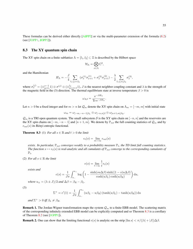
55

These formulas can be derived either directly [AJPP2] or via the multi-parameter extension of the formula (8.2)(see [JOPP1, JOPP2]).

8.3 The XY quantum spin chain

The XY spin chain on a finite sublattice Λ = [l1, l2] ⊂ Z is described by the Hilbert space

HΛ =⊗x∈Λ

C2,

and the HamiltonianHΛ = −J

4

∑l1≤x<l2

(σ(1)x σ

(1)x+1 + σ(2)

x σ(2)x+1)− λ

2

∑l1≤x≤l2

σ(3)x ,

where σ(j)x = (⊗x−1

y=l11)⊗ σ(j) ⊗ (⊗l2y=x+11), J is the nearest neighbor coupling constant and λ is the strength of

the magnetic field in the (3) direction. The thermal equilibrium state at inverse temperature β > 0 is

ωΛβ =e−βHΛ

Tr e−βHΛ.

Let n > 0 be a fixed integer and for m > n let Qm denote the XY spin chain on Λm = [−m,m] with initial state

ωm = ω[−m,−n−1]βL ⊗ ω[−n,n]β ⊗ ω[n+1,m]βR .

Qm is a TRI open quantum system. The small subsystem S is the XY spin chain on [−n, n] and the reservoirs arethe XY spin chains on [−m,−n− 1] and [n+ 1,m]. We denote by Pmt the full counting statistics of Qm and byemt(s) its Rényi entropic functional.

Theorem 8.3 (1) For all s ∈ R and t > 0 the limit

et(s) = limm→∞

emt(s)

exists. In particular, Pmt converges weakly to a probability measure Pt, the TD limit full counting statistics.The function s 7→ et(s) is real-analytic and all cumulants of Pmt converge to the corresponding cumulants ofPt.

(2) For all s ∈ R the limit

e(s) = limt→∞

1tet(s)

exists and

e(s) =1Jπ

∫ u+

u−

log(

1− sinh(su∆β) sinh((1− s)u∆β)cosh(uβL) cosh(uβR)

)du,

where u± = (λ± J)/2 and ∆β = βR − βL.

(3)

Σ+ = e′(1) =1Jπ

∫ u+

u−

(uβL − uβR) (tanh(uβL)− tanh(uβR)) du

and Σ+ > 0 iff βL 6= βR.

Remark 1. The Jordan-Wigner transformation maps the system Qm to a finite EBB model. The scattering matrixof the corresponding infinitely extended EBB model can be explicitly computed and so Theorem 8.3 is a corollaryof Theorem 8.2 (see [JOPP1]).

Remark 2. One can show that the limiting functional e(s) is analytic on the strip |Im s| < π/(|λ|+ |J |)∆β.

56

References

[Ab] Abou Salem, W.K.: On the quasi-static evolution of nonequilibrium steady states. Ann. H. Poincaré 8,569 (2007).

[AF] Abou Salem, W.K. and Fröhlich, J.: Cyclic thermodynamic processes and entropy production. J. Stat.Phys. 126, 431 (2007).

[Ar1] Araki, H.: Relative entropy of states of von Neumann algebras. Publ. Res. Inst. Math. Sci. Kyoto Univ.11, 809 (1975/76).

[Ar2] Araki, H.: Relative entropy of states of von Neumann algebras II. Publ. Res. Inst. Math. Sci. KyotoUniv. 13, 173 (1977/78).

[Ar3] Araki, H.: Relative Hamiltonian for faithful normal states of a von Neumann algebra. Publ. Res. Inst.Math. Sci. Kyoto Univ. 9, 165 (1973).

[AM] Araki, H. and Masuda, T.: Positive cones and Lp-spaces for von Neumann algebras. Publ. Res. Inst.Math. Sci. Kyoto Univ. 18, 339 (1982).

[AP] Aschbacher, W. and Pillet, C-A.: Non-equilibrium steady states of the XY chain. J. Stat. Phys. 112,1153 (2003).

[AJPP1] Aschbacher, W., Jakšic, V., Pautrat, Y. and Pillet, C.-A.: Topics in non-equilibrium quantum statisticalmechanics. In Open Quantum Systems III. Recent Developments. S. Attal, A. Joye and C.-A. Pilleteditors. Lecture Notes in Mathematics 1882, Springer, Berlin (2006).

[AJPP2] Aschbacher, W., Jakšic, V., Pautrat, Y. and Pillet, C.-A.: Transport properties of quasi-free fermions. J.Math. Phys. 48, 032101 (2007).

[ACM] Audenaert, K.M.R. et al.: Discriminating States: The Quantum Chernoff Bound. Phys. Rev. Lett. 98,160501 (2007).

[ANS] Audenaert, K.M.R., Nussbaum, M., Szkoła, A. and Verstraete, F.: Asymptotic error rates in quantumhypothesis testing. Commun. Math. Phys. 279, 251 (2008).

[BDK1] Bjelakovic, I. et al.: The Shannon-McMillan theorem for ergodic quantum lattice systems. Invent. Math.155 (2004)

[BDK2] Bjelakovic, I. et al.: A quantum version of Sanov’s theorem. Commun. Math. Phys. 260, 659 (2005).

[BDK3] Bjelakovic, I. et al.: Typical support and Sanov large deviations of correlated states. Commun. Math.Phys. 279, 559 (2008).

[Bl] Blahut, R.E.: Hypothesis testing and information theory. IEEE Trans. Inf. Theory 20, 405 (1974).

[BR1] Bratteli, O. and Robinson, D. W.: Operator Algebras and Quantum Statistical Mechanics 1. Springer,Berlin (1987).

[BR2] Bratteli, O. and Robinson D. W.: Operator Algebras and Quantum Statistical Mechanics 2. Springer,Berlin (1996).

[Br] Bryc, W.: A remark on the connection between the large deviation principle and the central limittheorem. Stat. Prob. Lett. 18, 253 (1993).

57

[Ch] Chernoff, H.: A measure of asymptotic efficiency for tests of a hypothesis based on the sum of observa-tions. Ann. Math. Stat. 23, 493 (1952)

[CL] Csiszár I. and Longo, G.: On the error exponent for source coding and for testing. simple statisticalhypotheses. Studia Sci. Math. Hungarica 6, 181 (1971).

[Dav] Davies, E.B.: Markovian master equations. Commun. Math. Phys. 39, 91 (1974).

[DS] Davies, E.B., and Spohn, H.: Open quantum systems with time-dependent Hamiltonians and their linearresponse. J. Stat. Phys. 19, 511 (1978).

[DZ] Dembo, A. and Zeitouni, O.: Large deviations techniques and applications. Second edition. Applica-tions of Mathematics, 38. Springer, New York (1998).

[DJP] Derezinski, J., Jakšic, V. and Pillet, C.-A.: Perturbation theory of W ∗-dynamics, KMS-states andLiouvillean. Rev. Math. Phys. 15, 447 (2003).

[El] Ellis, R.S.: Entropy, large deviations, and statistical mechanics. Springer, Berlin (1985). Reprinted inthe series Classics of Mathematics (2006).

[FMS] Fröhlich, J., Merkli, M., Schwarz, S. and Ueltschi, D.: Statistical mechanics of thermodynamic pro-cesses. A garden of quanta, 345 , World Sci. Publ., River Edge, NJ, (2003).

[FMU] Fröhlich, J., Merkli, M. and Ueltschi, D.: Dissipative transport: thermal contacts and tunnelling junc-tions. Ann. H. Poincaré 4, 897 (2003).

[Ha1] Hayashi, M.: Optimal sequence of quantum measurements in the sense of Stein’s lemma in quantumhypothesis testing. J. Phys. A. 35, 10759 (2002).

[Ha2] Hayashi, M.: Error exponent in asymmetric quantum hypothesis testing and its application to classical-quantum channel coding. Phys. Rev. A 76, 0623301 (2007).

[HP] Hiai, F. and Petz, D.: The proper formula for relative entropy and its asymptotics in quantum probability.Commun. Math. Phys. 143, 99 (1991).

[HMO1] Hiai, F., Mosonyi, M. and Ogawa, T: Large deviations and Chernoff bound for certain correlated stateson the spin chain. J. Math. Phys. 48, 123301 (2007).

[HMO2] Hiai, F., Mosonyi, M. and Ogawa, T: Error exponents in hypothesis testing for correlated states on aspin chain. J. Math. Phys. 49, 032112 (2008).

[HMO3] Hiai, F., Mosonyi, M., Ogawa, T. and Fannes, M.: Asymptotic distinguishability measures for shift-invariant quasi-free states of fermionic lattice systems. J. Math. Phys. 49, 072104 (2008).

[Ho] Hoeffding, H.: Asymptotically optimal tests for multinomial distributions. Ann. Math. Statist. 36, 369(1965).

[Is] Israel, R.: Convexity in the Theory of Lattice Gases. Princeton University Press, Princeton (1979).

[JKP] Jakšic, V., Kritchevski, E. and Pillet, C.-A.: Mathematical theory of the Wigner-Weisskopf atom. InLarge Coulomb systems. J. Derezinski and H. Siedentop editors. Lecture Notes in Physics 695, Springer,Berlin, (2006),

[JOP1] Jakšic, V., Ogata, Y. and Pillet, C.-A.: The Green-Kubo formula and the Onsager reciprocity relationsin quantum statistical mechanics. Commun. Math. Phys. 265, 721 (2006).

58

[JOP2] Jakšic, V., Ogata, Y. and Pillet, C.-A.: Linear response theory for thermally driven quantum opensystems. J. Stat. Phys. 123, 547 (2006).

[JOP3] Jakšic, V., Ogata, Y. and Pillet, C.-A.: The Green-Kubo formula for the spin-fermion system. Commun.Math. Phys. 268, 369 (2006).

[JOP4] Jakšic, V., Ogata, Y. and Pillet, C.-A.: The Green-Kubo formula for locally interacting fermionic opensystems. Ann. H. Poincaré 8, 1013 (2007).

[JP1] Jakšic, V. and Pillet, C.-A.: On entropy production in quantum statistical mechanics. Commun. Math.Phys. 217, 285 (2001).

[JP2] Jakšic, V. and Pillet, C.-A.: Mathematical theory of non-equilibrium quantum statistical mechanics. J.Stat. Phys. 108, 787 (2002).

[JP3] Jakšic, V. and Pillet, C.-A.: Non-equilibrium steady states of finite quantum systems coupled to thermalreservoirs. Commun. Math. Phys. 226, 131 (2002).

[JP4] Jakšic, V. and Pillet, C.-A.: On the strict positivity of entropy production. In Adventures in mathematicalphysics. F. Germinet and P.D. Hislop editors. Contemp. Math. 447, Amer. Math. Soc., Providence, RI,(2007).

[JPR] Jakšic, V., Pillet, C.-A. and Rey-Bellet, L.: Entropic fluctuations in statistical mechanics: I. Classicaldynamical systems. Nonlinearity 24, 699 (2011).

[JOPP1] Jakšic, V., Ogata, Y., Pautrat, Y. and Pillet, C.-A.: Entropic fluctuations in quantum statistical mechanics.An introduction. To appear in the Proceedings of the Les Houches School of Physics, held in LesHouches, Haute-Savoie in 2010.

[JOPP2] Jakšic, V., Ogata, Y., Pautrat, Y. and Pillet, C.-A.: Entropic fluctuations in statistical mechanics: II.Quantum dynamical systems. In preparation

[Ka] Kargin, V.: On the Chernoff distance for efficiency of quantum hypothesis testing. Ann. Statist. 33, 959(2005).

[Kub] Kubo, R.: Statistical-mechanical theory of irreversible processes. I. General theory and simple applica-tions to magnetic and conduction problems. J. Phys. Soc. Jap. 12, 570 (1957).

[KTH] Kubo, R., Toda, M. and Hashitsume, N.: Statistical physics. II. Nonequilibrium statistical mechanics.Second edition. Springer Series in Solid-State Sciences, 31. Springer, Berlin (1991).

[LS] Lebowitz, J.L. and Spohn, H.: Irreversible thermodynamics for quantum systems weakly coupled tothermal reservoirs. Adv. Chem. Phys. 38, 109 (1978).

[LR] Lehmann, E.L. and Romano, J.P.: Testing Statistical Hypotheses. Springer, New York (2005).

[LRB] Lenci, M. and Rey-Bellet, L.: Large deviations in quantum lattice systems: one-phase region. J. Stat.Phys. 119, 715 (2005).

[LL] Levitov, L.S. and Lesovik, G.B.: Charge distribution in quantum shot noise. JETP Lett. 58, 230 (1993).

[LiR] Lieb, E.H. and Ruskai, M.B.: Proof of the Strong Subadditivity of Quantum-Mechanical Entropy. J.Math. Phys. 14, 1938 (1973).

[MO] Matsui, T. and Ogata, Y.: Variational principle for non-equilibrium steady states of the XX model. Rev.Math. Phys. 15, 905 (2003).

59

[Me] Merhav, N.: Statistical Physics and Information Theory. Foundations and Trends in Communicationsand Information Theory 6, (2009). Now Publishers, Hanover, MA.

[MMS1] Merkli, M., Mück, M. and Sigal, I.: Theory of non-equilibrium stationary states as a theory of reso-nances. Ann. H. Poincaré 8, 1539 (2007).

[MMS2] Merkli, M., Mück, M. and Sigal, I.: Instability of equilibrium states for coupled heat reservoirs atdifferent temperatures. J. Funct. Anal. 243, 87 (2007).

[Mo] Mosonyi, M.: Hypothesis testing for Gaussian states on bosonic lattices. J. Math. Phys. 50, 032105(2009).

[MHO] Mosonyi, M., Hiai, F., Ogawa, T. and Fannes, M.: Asymptotic distinguishability measures for shift-invariant quasifree states of fermionic lattice systems. J. Math. Phys. 49, 072104 (2008).

[Na] Nagaoka, H.: Strong converse theorems in quantum information theory. In Asymptotic Theory ofQuantum Statistical Inference. M. Hayashi editor. World Scientific, Singapore (2005).

[NR] Netocný, K. and Redig, F.: Large deviations in quantum spin systems. J. Stat. Phys. 117, 521 (2004).

[NS1] Nussbaum, M. and Szkoła A.: Exponential error rates in multiple state discrimination on a quantumspin chain. J. Math. Phys. 51, 072203 (2010).

[NS2] Nussbaum, M. and Szkoła, A.: The Chernoff lower bound for symmetric quantum hypothesis testing.Ann. Stat. 37, 1057 (2009).

[Og1] Ogata, Y.: The stability of the non-equilibrium steady states. Commun. Math. Phys. 245, 577 (2004).

[Og2] Ogata, Y.: Large deviations in quantum spin chains. Commun. Math. Phys. 296, 35 (2010).

[Og3] Ogata, Y.: A Generalization of Powers–Størmer Inequality. Lett. Math. Phys. 97, 339 (2011).

[OH] Ogawa, T. and Hayashi, M.: On error exponents in quantum hypothesis testing. IEEE Trans. Inf. Theory50, 1368 (2004).

[ON] Ogawa, T. and Nagaoka, H.: Strong converse and Stein’s lemma in quantum hypothesis testing. IEEETrans. Inf. Theory 46, 2428 (2000).

[OP] Ohya, M. and Petz, D.: Quantum Entropy and Its Use. Second edition. Springer, Berlin (2004).

[Pe] Pearson, K.: On the criterion that a given system of deviations from the probable in the case of acorrelated system of variables is such that it can be reasonably supposed to have arisen from randomsampling. Phil. Mag. Ser. 5, 50, 157, (1900).

[Pi] Pillet, C.-A.: Entropy production in classical and quantum systems. Markov Process. Related Fields 7,145 (2001).

[Re] Rényi, A.: On measures of information and entropy. In Proc. 4th Berkeley Sympos. Math. Statist. andProb., Vol. I, Univ. California Press, Berkeley (1961).

[R] Rockafellar, R.T.: Convex Analysis. Princeton University Press, Princeton, NJ (1972).

[Ro] de Roeck, W.: Large deviation generating function for currents in the Pauli-Fierz model. Rev. Math.Phys. 21, 549 (2009).

[Ru1] Ruelle, D.: Entropy production in quantum spin systems. Commun. Math. Phys. 224 (2001).

60

[Ru2] Ruelle, D.: How should one define entropy production for nonequilibrium quantum spin systems? Rev.Math. Phys. 14, 701 (2002).

[Si] Simon, B.: Statistical Mechanics of Lattice Gases. Princeton University Press, Princeton (1993).

[St] Stratila, S, .: Modular Theory in Operator Algebras. Abacus Press, Turnbridge Wells (1981).

[Tak] Takesaki, M.: Theory of Operator Algebras I. Springer, New-York (1979).

[Tas] Tasaki, S.: On entropy production of a one-dimensional lattice conductor. In Quantum information V.T. Hida and K. Saitô editors. World Scientific, Singapore (2006).

[TM1] Tasaki, S. and Matsui, T.: Fluctuation theorem, non-equilibrium steady states and Maclennan-Zubarevensembles of a class of large systems. In Fundamental Aspects of Quantum Physics. L. Accardi andS. Tasaki editors. QP-PQ: Quantum Probability and White Noise Analysis 17. World Scientific, Singa-pore (2003).

[TM2] Matsui, T. and Tasaki, S.: Nonequilibrium steady states with Bose-Einstein condensates. In StochasticAnalysis: Classical and Quantum. T. Hida editor. World Scientific, Singapore (2005).

[Uh] Uhlmann, A.: Relative entropy and the Wigner-Yanase-Dyson-Lieb concavity in an interpolation theory.Commun. Math. Phys. 54, 123 (1977).

Quantum Hypothesis Testing and Non-Equilibrium Statistical ... · Quantum Hypothesis Testing and...

Documents

Transcript of Quantum Hypothesis Testing and Non-Equilibrium Statistical ... · Quantum Hypothesis Testing and...