Quantum Finance-Schrodinger's Eq Applied to Stock … Word - Quantum Finance-Schrodinger's Eq...

Schrodinger’s Equation and the Financial Markets By: Alex Marshall

1

Introduction:

The new interdisciplinary research field that the methodological approaches and analogizes physical theories to the economic world, Econophysics, incepted from an overall lack in effective analytical models in Economics. This is because of Economist historical route of encountering problem has instilled itself to this day; sadly, the social science has not always had the available empirical data it has today, which in result, led to a discipline founded and perpetuated by theorist. As for hard sciences, theorists are dependent upon experimentalist, and conversely, by definition, an experiment is a procedure done in order to test a hypothesis. Today, Economics is sitting on a plethora of data, but lacks the necessary interdependence of those who theorize and those who rigorously investigate the hypothesis. Econophysics has come to see success with focusing on a scientific approach to explaining Economic phenomena, but their greatest achievement to date is with Quantum Finance.

The Black-‐Scholes Model:

One of the most important concepts in modern financial theory was stumbled upon by Fisher Black, and aided by Myron Scholes, when they derived a differential equation, the Black-‐Scholes model, to solve the fair-‐price of options, which resembled the heat equation (Rubash, n.d.). An option is basically just a contract that legally gives the owner of the contract, the ability to buy or sell a stock, if it reaches a predetermined price (strike price) before the specified date on the contract, known as a “call” and “put,” respectively. Due to the nature of the option being risky, the purchaser of the contract pays at a premium price, which is why there is a need for models that can value the option.

Up until 1973, when the Black-‐Scholes model was created, there was not an effective way of call option pricing. Their model is as shown (Stock 500, 2005):

EQ 1

𝑤 = 𝑆 ∗ 𝑁ln S

K + 𝑟 + 𝑠!

2 𝑡

𝑠 𝑡− 𝐾𝑒!!"𝑁

ln SK + 𝑟 + 𝑠

!

2 𝑡

𝑠 𝑡− 𝑠 𝑡

Where,

w = Theoretical Call Premium

S = Current Stock Price


2

t = time until expiration

K = striking price

r = risk-‐free interest rate

N = Cumulative standard normal distribution

Even though the initial model was one that carved the way of option valuation in Financial Theory, it was still weak because of a lack of dynamism: there are assumptions of continuous trading, constant volatility, constant interest rate, and that the market is efficient.

Today, many of the assumptions of the model have been removed or made more dynamic through extensions. Many stocks are observed to move between bounds, which can be used to maximize profits. The lower price barrier of a stock is the “support” and can be defined as a price level that historically, the stock has trouble falling under; as for the upper limit, it is called a “resistance” and this is a price level that in the past doesn’t rise above. The resistance can be observed in Figure 1 of Kohl’s Stock:

Figure 1 (Rubash, n.d.):

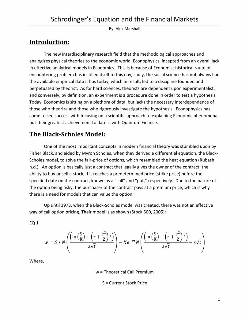
There are two scenarios that occur when the stock reaches either of the bounds: they will reach either level and change direction or they will penetrate the barrier and find “find another level of support” (Rubash, n.d.). This phenomenon can be seen in Boeing’s Stock in Figure 1:


3


The next graphic has a superb depiction of the barrier: when the support barrier is broken, it becomes the new resistance barrier, vis versa. Figure 3 represents the stocks for Burlington Northern Santa Fe Corp:



4

The Schrodinger Equation:

These barriers are intuitively able to be analogous to potential energy barriers; therefore, we can find the probability that the stock will penetrate the barriers the with the Black-‐Scholes model with the method of separation of variables, which is allowed because the stationary price is bound by the support and resistance price levels. Solving the model will result in two solutions: a time-‐independent and a time dependent formula. We will investigate the time-‐independent equation because it is representative of a one-‐dimensional Schrodinger equation used for a particle in a box. From there, the penetration of the barriers will result in a tunneling of the stock. From here on out, the method for solving the Black-‐Scholes model is based off of Racorean’s.

To begin, the general partial differential Black-‐Scholes equation can be written as (Racorean, n.d.):

EQ 2

𝜕𝑤𝜕𝑡 = −

12𝜎

!𝑆!𝜕!𝑤𝜕𝑆! − 𝑟𝑆

𝜕𝑤𝜕𝑡 + 𝑟𝑤


5

Where,

w = Theoretical Call Premium

S = Current Stock Price

t = time until expiration

K = striking price

r = risk-‐free interest rate

𝜎 = Volatility of the stock

Equation 2 can be solved with the method of separation of variables and results in a product of two functions:

EQ 3

𝑤 𝑆, 𝑡 = ∅(𝑆)𝜑(𝑡)

Now, combine equation 2 and equation 3, while changing the partial derivatives to ordinary derivatives:

EQ 4

𝑑𝜑 𝑡𝑑𝑡

1𝜑 𝑡 = −

12𝜎

!𝑆!𝑑!∅ 𝑆𝑑𝑆!

1∅ 𝑆 − 𝑟𝑆

𝑑∅ 𝑆𝑑𝑆

1∅(𝑆)+ 𝑟

Therefore, each side of the equation must equal a constant λ:

EQ 5

𝑑𝜑 𝑡𝑑𝑡

1𝜑 𝑡 = λ

EQ 6

λ = −12𝜎

!𝑆!𝑑!∅ 𝑆𝑑𝑆!

1∅ 𝑆 − 𝑟𝑆

𝑑∅ 𝑆𝑑𝑆

1∅(𝑆)+ 𝑟

In order to find Α, the time-‐dependency is used:


6

EQ 7

𝑑𝜑 𝑡𝑑𝑡 = λ𝜑 𝑡

Therefore:

EQ 8 𝜑 𝑡 = 𝑒!!

From here, economic reasoning is the determinant of the constant, which is circumstantial. The previous equation shoes the time dependency of option price, but since the option value decreases over time, λ has to be negative. Also, because option price decays quickly with low volatility and at a slow pace with high volatility, the constant must include 𝜎. Finally, the interest rate is another influential factor, which in high interest leads to small movements in the stock market, whereas, low interest rate leads to major movements in the stock market. Therefore, the rate of decay in the option price over time is:

EQ 9

𝜑 𝑡 = 𝑒!!!!

Now, the range bounds can be derived with equation 6, the time-‐independence in the form:

EQ 10

∅ 𝑆 λ = −12𝜎

!𝑆!𝑑!∅ 𝑆𝑑𝑆! − 𝑟𝑆

𝑑∅ 𝑆𝑑𝑆 + 𝑟

The homogeneous part can be written as:

EQ 11

0 = 𝑑!∅ 𝑆𝑑𝑆! −

2𝑟𝜎!𝑆

𝑑∅ 𝑆𝑑𝑆 −

2𝑟𝜎!𝑆! ∅ 𝑆

Using the notation, ln∅ 𝑆 = ln 𝜓 𝑆 − !!

!!!!!

𝑑𝑆, equation 11 can be written as:


7

EQ 12

0 = 𝑑!𝜓 𝑆𝑑𝑆! −

𝑟𝜎!𝑆! (1+

𝑟𝜎!) 𝜓 𝑆

Therefore,

EQ 13

−𝜎!

𝑟 𝜎! + 𝑟 𝑑!𝜓 𝑆𝑑𝑆! +

1𝑆! 𝜓 𝑆 = 0

This is the zero energy particle time-‐independent Schrodinger equation with the potential:

EQ 14

𝑉(𝑆) =1𝑆!

Therefore, the shape of the potential is shown in the figure below. As the stock price, S, increases, the potential V(s) reduces, but will never reach zero and the wall becomes thicker. Also, since there is no constant λ, the stock cannot leave the well:



8

Where,

𝑆𝑡𝑜𝑐𝑘 𝑝𝑟𝑖𝑐𝑒, 𝑆, 𝑖𝑠 𝑡ℎ𝑒 𝑧𝑒𝑟𝑜𝑡ℎ

𝑆𝑡𝑟𝑖𝑘𝑒 𝑝𝑟𝑖𝑐𝑒,𝐾, 𝑖𝑠 𝑜𝑛 𝑡ℎ𝑒 𝑟𝑒𝑠𝑖𝑠𝑡𝑎𝑛𝑐𝑒 𝑙𝑒𝑣𝑒𝑙 𝑎𝑛𝑑 𝑖𝑠 𝑡ℎ𝑒 𝑤𝑖𝑑𝑡ℎ 𝑜𝑓 𝑡ℎ𝑒 𝑏𝑜𝑥

𝑇ℎ𝑒 𝑝𝑜𝑡𝑒𝑛𝑡𝑖𝑎𝑙 𝑟𝑒𝑠𝑡𝑖𝑠𝑡𝑎𝑛𝑐𝑒 𝑙𝑒𝑣𝑒𝑙 𝑝𝑟𝑖𝑐𝑒 𝑙𝑒𝑣𝑒𝑙 𝑖𝑠 𝑉!,

EQ 15

𝑉! =1𝐾!

Since λ must be a part of our equation to observe penetration. Therefore, using equation 10, equation 12, and equation 15:

EQ 16

−𝜎!

𝑟 𝜎! + 𝑟 𝑑!𝜓 𝑆𝑑𝑆! + 𝑉(𝑆)𝜓 𝑆 = λ𝜓 𝑆


9

We already know what the constant is:

EQ 17

−𝜎!

𝑟 𝜎! + 𝑟 𝑑!𝜓 𝑆𝑑𝑆! + 𝑉 𝑆 𝜓 𝑆 = 𝜓 𝑆

r𝜎

Thus:

EQ 18

𝜓 𝑆 = 2𝐾 sin 𝑛𝜋

𝑆𝐾

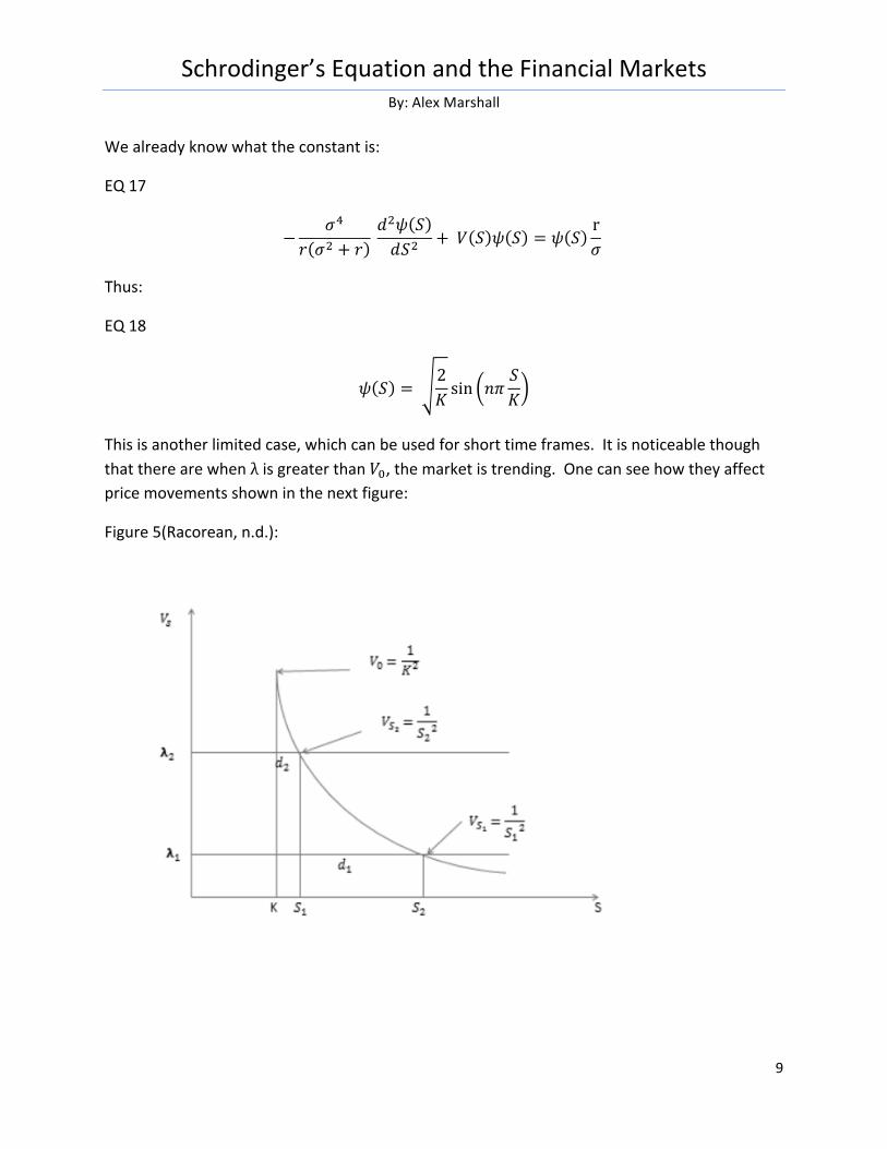
This is another limited case, which can be used for short time frames. It is noticeable though that there are when λ is greater than 𝑉!, the market is trending. One can see how they affect price movements shown in the next figure:

Figure 5(Racorean, n.d.):


10

Now, with constant time decay, λ, for the option valuation, it does two affects: it reduces the option price over time and shifts the option value impact the stock market itself. Now for when the time decay is conditioned as being less than the potential.

Apparent from figure 5, when interest rate is high or the volatility is low, the thinner the wall width; therefore, with these conditions, even marginal shifts in stock price would penetrate the wall and tunnel. Thus, higher the interest rate, lower the expectancy of big movements.

Additionally, when interest rate is low or the volatility is high, the greater the wall width; therefore, large shifts in stock price, will penetrate the wall. Thus, lower the interest rate, higher the expectancy of big movements.

Finally, when the decay is constant, we know 𝜆 < 𝑉! and equation 15:

EQ 19

𝐾 <1𝜆

Therefore, if we know the time constant, we can forecast the magnitude of the shift. Observing figure 5 again, denoting the potential Vr as the potential at the boundary of the wall, we know that 𝜆 must be equal to it; therefore, the stock at the boundary is:

EQ 20

𝑆! =1𝜆

Thus, the penetration distance, d, is the distance between the strike price and the tunneling stock is:

EQ 21

𝑑 = 𝑆! − 𝐾 =1𝜆 − 𝐾 =

𝜎𝑟 − 𝐾


11

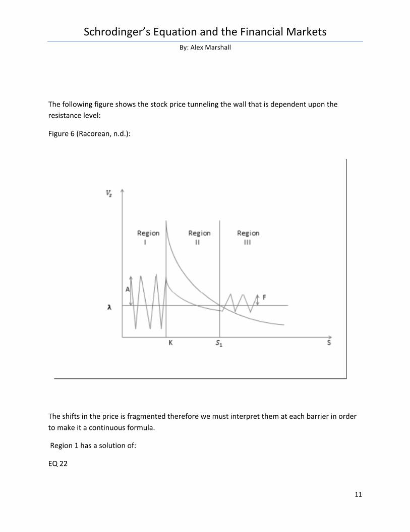
The following figure shows the stock price tunneling the wall that is dependent upon the resistance level:

Figure 6 (Racorean, n.d.):

The shifts in the price is fragmented therefore we must interpret them at each barrier in order to make it a continuous formula.

Region 1 has a solution of:

EQ 22


12

𝜓! = 𝐴𝑒!"# + 𝐵𝑒!!"#

Where,

𝑘 = 𝑟𝜎! (𝜎

! + 𝑟)𝜆


EQ 23

𝜓! = 𝐶𝑒!" + 𝐷𝑒!!"

Where,

𝑞 = 𝑟𝜎! (𝜎

! + 𝑟)(𝑉 𝑠 − 𝜆)


EQ 24

𝜓! = 𝐹𝑒!"#

Therefore, the probability for the stock price tunneling through the entire barrier is, T:

EQ 25

𝑇 =𝐹 !

𝐴 !

Thus:

EQ 26


13

𝐴 ! = 𝐹 !(((𝑘! + 𝑞!)^24𝑘!𝑞! sinh!(𝑞𝑑)+ 1)

Then, in terms of V and 𝜆:

EQ 27

𝑇 =𝑉!

4𝜆 𝑉 − 𝜆 sinh! 𝑞𝑑 + 1!!

For qd>>1, the sinh term overwhelms the rest, therefore, this can be approx. be:

EQ28

𝑇 = 𝑒!!!"

All possible barrier potential solutions:

EQ29

𝑇 = 𝑒!! !"#"

The sum replaced with an integral is:

EQ 30

𝑇 = 𝑒!! !

!! !!!! !

!!!!"#!!!

EQ31

𝑇 = 𝑒!! !

!! !!!! !

! !"!!!!!!!!!!!!!!

! !!!!!

Since we know𝜆 = !!,

EQ32

𝑇 = 𝑒!! !

!! !!!! !

! !"!!!!!

!!!

!!!!!!!!

! !!!!!!

This is the final probability of the stock penetrating through the walls! I will not be doing any empirical research, but Racorean does a strong job doing so (Racorean, n.d.)


14

Conclusion:

With the derived solutions, the tunneling is actualized, when interest rate is constant, the wall must be thin, which in turn leads to a relatively small volatility. Basically, in order for the tunneling to even occur, there needs to be a rapid fall in the stock volatility. This phenomena in the financial market is nearly identical to a quantum physics, resistance and support are two common occurrences in the stock market and the way in they affect the stock’s movement can be explained through a Quantum Physics tunneling effect. Financial Analyst and investors are capable of using these tools in order to gain information in almost a predictive manner. Overall, the Schrodinger equation is much more versatile than just being a Quantum model and henceforth, there are many different applications of Physical solutions than just to the physical world; by this I mean, if a route of how we understand the Quantum world is applicable to the Financial Industry, then where are the limits of applying rigorous Physics solutions, in an analogous manner, to other disciplines problems, to further humankind on all fronts.


15

Further Reading/References:

Learn Stock Options Trading. N.d. Using Support and Resistance. Learn Stop Options Trading. Retreived from: http://www.learn-‐stock-‐options-‐trading.com/support-‐and-‐resistance.html

Racorean, Ovidiu. N.d. Time-‐independent pricing of options in range bound markets. Arxiv. Retrieved from: http://arxiv.org/ftp/arxiv/papers/1304/1304.6846.pdf

Rubash, Kevin. N.d. A Study of Option Pricing Models. Bradley University. Retrieved from: http://bradley.bradley.edu/~arr/bsm/pg04.html

Stock 500. 2005. What is an Option Contract? Morningstar. Retrieved from: http://news.morningstar.com/classroom2/course.asp?docId=145386&page=3&CN=

Quantum Finance-Schrodinger's Eq Applied to Stock … Word - Quantum Finance-Schrodinger's Eq...

Documents

Transcript of Quantum Finance-Schrodinger's Eq Applied to Stock … Word - Quantum Finance-Schrodinger's Eq...