quantum filtering and smoothing theory productskyodo/kokyuroku/contents/pdf/...An invitation to...
27
An invitation to quantum filtering and smoothing theory based on two inner products By Kentaro OHKI * Abstract The purpose of this paper is to introduce the quantum filtering and a smoothing theory for Markovian open quantum dynamical systems briefly. The filtering and smoothing theory for classical systems are well developed and show their performance used in practice, and the quantum filtering theory has also developed from 1980\mathrm{s} based on the quantum version of the classical conditional expectation. However, the quantum smoothing theory has not developed since the quantum conditional expectation is not defined as well. We developed a quantum smoothing theory based on two quantum inner products and show it with the filtering theory. The weak value is naturally defined as the minimum mean square estimate in our frame work and the quantum smoother, the dynamical estimator of weak value, is derived. §1. Introduction State estimation problems of dynamical systems driven by noisy disturbances often arise in practice, and many kinds of estimators are proposed to extract the exact signal from noisy observations [30, 49, 50, 56, 60]. A state estimation problem is a problem that reconstruction of the objective, such as parameters of a probability density function and physical quantities, from measured data (Fig. 1). One of the central notions of state estimations is the \mathrm{s}\mathrm{c}\succ called minimum mean squares estimation and it is widely used because it is intuitive and easy to obtain the optimal solution by Hilbert space theory [6, 38, 40]. Despite the first study of the minimum mean squares estimation problems was found in 1700\mathrm{s}[51] , it has been studied and developed so far; for examples, a relation between estimation errors and mutual information is found and developed in [17, 28, 29, 57], Received April 20, 201\mathrm{x} . Revised September 11, 201\mathrm{x}. 2010 Mathematics Subject Classification(s): Key Words: Quantum filtering theory, Quantum smoothing theory * Graduate School of inforrnatics, Kyoto University, Kyoto 606‐8501, Japan. \mathrm{e}‐mail: ohkiOi. kyoto‐u. ac. jp 数理解析研究所講究録 第2018巻 2017年 18-44 18
Transcript of quantum filtering and smoothing theory productskyodo/kokyuroku/contents/pdf/...An invitation to...

An invitation to quantum filtering and smoothingtheory based on two inner products
By
Kentaro OHKI *
Abstract
The purpose of this paper is to introduce the quantum filtering and a smoothing theoryfor Markovian open quantum dynamical systems briefly. The filtering and smoothing theoryfor classical systems are well developed and show their performance used in practice, and the
quantum filtering theory has also developed from 1980\mathrm{s} based on the quantum version of the
classical conditional expectation. However, the quantum smoothing theory has not developedsince the quantum conditional expectation is not defined as well. We developed a quantum
smoothing theory based on two quantum inner products and show it with the filtering theory.The weak value is naturally defined as the minimum mean square estimate in our frame work
and the quantum smoother, the dynamical estimator of weak value, is derived.
§1. Introduction
State estimation problems of dynamical systems driven by noisy disturbances often
arise in practice, and many kinds of estimators are proposed to extract the exact signalfrom noisy observations [30, 49, 50, 56, 60]. A state estimation problem is a problemthat reconstruction of the objective, such as parameters of a probability density function
and physical quantities, from measured data (Fig. 1). One of the central notions of
state estimations is the \mathrm{s}\mathrm{c}\succ called minimum mean squares estimation and it is widelyused because it is intuitive and easy to obtain the optimal solution by Hilbert space
theory [6, 38, 40].Despite the first study of the minimum mean squares estimation problems was found
in 1700\mathrm{s}[51] , it has been studied and developed so far; for examples, a relation between
estimation errors and mutual information is found and developed in [17, 28, 29, 57],Received April 20, 201\mathrm{x} . Revised September 11, 201\mathrm{x}.
2010 Mathematics Subject Classification(s):Key Words: Quantum filtering theory, Quantum smoothing theory
* Graduate School of inforrnatics, Kyoto University, Kyoto 606‐8501, Japan.\mathrm{e}‐mail: ohkiOi. kyoto‐u. ac. jp
数理解析研究所講究録第2018巻 2017年 18-44
18

KENTARO OHKI
Figure 1. Abstract setting of estimation problems
and new estimators for dynamical systems described on certain manifolds, quantum
systems are derived [13, 14, 23]. The minimum mean square estimator is given by the
conditional expectation and we obtain a recursive estimator for hidden random variables
[38, 40]. First of \mathrm{a}\mathrm{J}1 , let us review the dynamical minimum mean square estimator
without rigorous descriptions. Consider a system driven by Wiener noise with noisymeasurement:
dX_{t}=f(X_{t})dt+g(X_{t})dW_{\mathrm{t}},
dY_{t}=h(X_{t})dt+dV_{t},
where all signals are one‐dimensional random variables at any time t\geq 0. W and V are
mutually independent one‐dimensional standard Wiener processes. The functions f, g
and h satisfy certain suitable conditions. Let C_{t} be a set of \mathcal{F}_{t} := $\sigma$(\{\mathrm{Y}_{s}|0\leq s\leq tmeasurable real‐valued functions and P be a probability measure of the whole signals.
Problem 1.1.
Find a function Q^{\mathrm{o}\mathrm{p}\mathrm{t}}\in C_{t} as a solution of the following minimization problem
\displaystyle \min_{Q\in C_{t}}\mathrm{E}_{P}[|X_{ $\tau$}-Q|^{2}],where \mathrm{E}_{P} is the expectation with respect to the probability measure P.
Problem 1.1 is called the prediction problem if \prime r>t , the filtering problem if $\tau$=t,
and the smoothing problem if $\tau$<t , respectively. Whether t is larger than $\tau$ or not,
the solution of Problem 1.1 is given Uy the Q^{\mathrm{o}\mathrm{p}\mathrm{t}}\in C_{t} satisfying
\mathrm{E}_{P}[(X_{ $\tau$}-Q^{\mathrm{o}\mathrm{p}\mathrm{t}})Z]=0, \forall Z\in C_{t}.
This implies that the estimation error and C_{t} are mutually orthogonal under the proba‐
bility measure P . The orthogonality defines the conditional expectation [11], and Q^{\mathrm{o}\mathrm{p}\mathrm{t}}
19
AN INVITATION TO QUANTUM FILTERING AND SMOOTHING THEORY BASED ON TWO INNER PRODUCTS
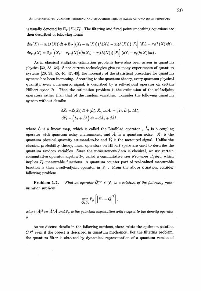
is usually denoted by \mathrm{E}_{P}[X_{ $\tau$}|\mathcal{F}_{t}] . The filtering and fixed point smoothing equations are
then described of following forms
d$\pi$_{t}(X)=$\pi$_{t}(f(X))dt+\mathbb{E}_{P}[(X_{t}-$\pi$_{t}(X))(h(X_{t})-$\pi$_{t}(h(X)))|\mathcal{F}_{t}](dY_{t}-$\pi$_{t}(h(X))dt) ,
d$\pi$_{ $\tau$|t}(X)=\mathrm{E}_{P}[(X_{ $\tau$}-$\pi$_{ $\tau$|t}(X))(h(X_{t})-$\pi$_{t}(h(X)))|\mathcal{F}_{t}](dY_{t}-$\pi$_{t}(h(X))dt) .
As in classical statistics, estimation problems have also been arisen in quantum
physics [32, 33, 34]. Since current technologies give us many experiments of quantum
systems [20, 39, 45, 46, 47, 48], the necessity of the statistical procedure for quantum
systems has been increasing. According to the quantum theory, every quantum physical
quantity, even a measured signal, is described by a self‐adjoint operator on certain
Hilbert space \mathcal{H} . Then the estimation problem is the estimation of the self‐adjointoperators rather than that of the random variables. Consider the following quantum
system without details:
d\hat{X}_{t}=\hat{\mathcal{L}}(\hat{X}_{t})dt+[\hat{L}_{t}^{*},\hat{X}_{t}]_{-}d\^{A}_{t}+[\hat{X}_{t}, \hat{L}_{t}] ‐dÂt* ,
d\hat{Y}_{t}=(\hat{L}_{t}+\hat{L}_{t}^{*})dt+d\hat{A}_{t}+d\hat{A}_{t}^{*},where \hat{\mathcal{L}} is a linear map, which is called the Lindblad operator, \hat{L}_{t} is a coupling
operator with quantum noisy environment, and \hat{A}_{t} is a quantum noise. X. is the
quantum physical quantity \mathrm{e}\mathrm{s}\mathrm{t}\mathrm{i}\mathrm{m}\mathrm{a}\mathrm{n}\mathrm{d}-\mathrm{t}\mathrm{c}\succ \mathrm{b}\mathrm{e} and Y. is the measured signal. Unlike the
classical probability theory, linear operators on Hilbert space are used to describe the
quantum random variables. Since the measurement data is classical, we use certain
commutative operator algebra \mathcal{Y}_{t} , called a commutative von Neumann algebra, which
implies \mathcal{F}_{t}‐measurable functions. A quantum counter part of real‐valued measurable
function is then a self‐adjoint operator in \mathcal{Y}_{t} From the above situation, consider
following problem.
Problem 1.2. Find an operator \hat{Q}^{\mathrm{o}\mathrm{p}\mathrm{t}}\in y_{t} as a solution of the following mini‐
mization problem
\hat{Q}\in \mathcal{Y}_{t}\mathrm{m}\mathrm{j}\mathrm{n}\mathbb{P}_{\hat{ $\rho$}}[|\hat{X}_{ $\tau$}-\hat{Q}|^{2}],where | Â | 2 : = Â*Â and \mathbb{P}_{\hat{ $\rho$}} is the quantum expectation with respect to the density operator
\hat{ $\rho$}.
As we discuss details in the following sections, there exists the optimum solution
\hat{Q}^{\mathrm{o}\mathrm{p}\mathrm{t}} even if the object is described in quantum mechanics. For the filtering problem,the quantum filter is obtained by dynamical representation of a quantum version of
20
KENTARO OHKI
conditional expectation [13, 14]. The optimal solution \hat{Q}^{\mathrm{o}\mathrm{p}\mathrm{t}} of the quantum filtering
problem satisfies the following orthogonality,
\mathbb{P}_{\hat{p}}[\hat{Z}(\hat{X}_{ $\tau$}-\hat{Q}^{\mathrm{o}\mathrm{p}\mathrm{t}})]=0, \forall\hat{Z}\in \mathcal{Y}_{t}, $\tau$=t.Usually the \hat{Q}^{\mathrm{o}\mathrm{p}\mathrm{t}} is denoted by \mathbb{P}_{\hat{ $\rho$}}[\hat{X}_{ $\tau$}|y_{t}] . Then the recursive filtering equation is
d\hat{ $\pi$}_{t}(\hat{X})=\hat{ $\pi$}_{t}(\hat{\mathcal{L}}(\hat{X}))dt+\mathbb{P}_{\hat{ $\rho$}}[(\hat{L}_{t}-\hat{ $\pi$}_{t}(\hat{L}))^{*}\hat{X}_{t}+\hat{X}_{t}(\hat{L}_{t}-\hat{ $\pi$}_{t}(\hat{L}))|\mathcal{Y}_{t}](d\hat{\mathrm{Y}}_{t}-\hat{ $\pi$}_{t}(\hat{L}+\hat{L}^{*})dt) ,
where \hat{ $\pi$}_{t}(\hat{X}):=\mathbb{P}_{\overline{ $\rho$}}[\hat{X}_{t}|\mathcal{Y}_{t}] is the quantum conditional expectation. The solutions of
quantum prediction and filtering problems are obtained by the quantum conditional
expectation [8, 13, 14] and the quantum conditional expectation is well‐defined if we
consider the indirect measurement [61]. The key notion why the quantum condi‐
tional expectation is well‐defined is the commutativity between measurement records
and physical quantities to be estimated, and it ensures a certain orthogonal condition
between estimation error and measurement records. The quantum filtering theory also
shed a light on the measurement‐Uased feedback control theory for quantum systems
[3, 9, 10, 21, 37, 61, 64].However, the solution of the general quantum smoothing problems is not described
by the quantum conditional expectation. In contrast to the classical random variables,
quantum random variables do not have the commutativity with respect to multiplica‐tion and the past physical quantities does not commute with the measurement records
in general. This makes ones impossible to define the quantum conditional expectation,
therefore, the general smoothing theory must not be based on the quantum condi‐
tional expectation. The previous work on quantum smoothing problems, Yanagisawafound that the quantum systems which smoothing problem is described by the quan‐
tum conditional expectation [62]. This work opened the door of the quantum smoothing
problems and several researches have tackled with the problems [25, 53, 54, 63]. For
example, Tsang also gave a smoothing method for a quantum phase estimation problem
[53], which is based on the time‐symmetric approach proposed by Aharonov et al. [2].Yonezawa et al. [63] gave another approach for the quantum optical‐phase estimation
and showed experimental results of the estimation problem. Since these estimation
problems are the estimation of the classical parameter in the quantum system, they end
up solving the classical smoothing problem. Recently Gammelmark et al. derived a new
past state estimation scheme [25] based on weak values [1, 22]. Furthermore, the author
of this paper proposed a new smoothing theory based on two inner products [42, 43],which is the main topic of this paper.
In this paper, we show the optimal solution \hat{Q}^{\mathrm{o}\mathrm{p}\mathrm{t}} of Problem 1.2 is composed of
two operators \hat{Q}^{\mathrm{o}\mathrm{p}\mathrm{t}}=\hat{Q}^{+}+\hat{Q}^{-}, where \hat{Q}^{+} and \hat{Q}^{-} satisfying the symmetric orthogonal
21

AN INVITATION TO QUANTUM FILTERING AND SMOOTHING THEORY BASED ON TWO INNER PRODUCTS
condition and the skew symmetric condition under a quantum state \hat{ $\rho$}
\mathbb{P}_{\hat{ $\rho$}}[\hat{Z}(\hat{X}_{ $\tau$}-\hat{Q}^{+})+(\hat{X}_{ $\tau$}-\hat{Q}^{+})\hat{Z}]=0,\mathbb{P}_{\hat{ $\rho$}}[\hat{Z}\hat{X}_{ $\tau$}-\hat{X}_{ $\tau$}\hat{Z}]=2\mathbb{P}_{\hat{ $\rho$}}[\hat{Q}^{-}\hat{Z}], \forall\hat{Z}\in y_{t},
respectively. We also show that \hat{Q}^{+} is the best approximation in the sense of symmetricinner product. The optimal solution \hat{Q}^{\mathrm{o}\mathrm{p}\mathrm{t}} coincides with the �weak value� of \hat{X}
, which
is well‐known in physics literatures [1, 18, 19, 22, 24]. Furthermore, we propose a new
framework for quantum smoothing theory based on the symmetric orthogonal condition.
This is a natural extension of the quantum conditional expectation and gives a recur‐
sive minimum mean square estimation for past quantum physical quantities. Recently,Amini et al. derived the hnear minimum mean squares estimator for linear quantum
systems [5] and the estimator is realized in quantum systems. Their estimator is inter‐
esting but it is impossible to estimate past quantum states because the implementedestimator is causal. Our proposal estimator is for general Markovian quantum systemsand realized in classical systems. It is possible to implement non‐causal estimator in
practice, so it is possible to estimate the past quantum states in principle.The rest of this paper is organized as follows. In Section 2, we introduce some
foundations of quantum theory and quantum statistics. Especially, we show the keyidea of the main result of this paper in finite dimensional quantum system. The concept
of this paper is described in this section. In Section 3, we introduce the symmetric
orthogonality and asymmetric condition and show that the operators satisfying these
conditions are the real part and imaginary part of the minimum mean square estimation.
The quantum dynamical system considered in this paper and its filter are shown in
Section 4. We develop a new quantum smoother in Section 5 and conclude this paper
in Section 6.
Notation
\mathbb{R} and \mathbb{C} are real numbers and complex numbers, respectively, and \mathrm{i} :=\sqrt{-1}. \mathcal{H} is
a complex Hilbert space and we also denote \mathcal{H}x if it is the Hilbert space of the systemX. Any hnear operator on a Hilbert space \mathcal{H} is denoted by hat, e.g., \hat{X} . When positive
operators \hat{X} and \hat{Y} satisfy \hat{X}=\hat{Y}^{2} , we denote \hat{\mathrm{Y}}=\sqrt{X} . The absolute value of operatoris defined by |\hat{X}| :=\sqrt{\hat{X}^{*}\hat{X}}. \mathcal{L}(\mathcal{H}) is the set of all linear bounded operators on the
Hilbert space \mathcal{H}.\hat{X}\geq 0 means that \hat{X}\in \mathcal{L}(\mathcal{H}) is a positive operator and \hat{X}^{*} implies the
conjugate operator of \hat{X} . Tr [] : \mathcal{L}(\mathcal{H})\rightarrow \mathbb{C} is the trace on the linear bounded operators.
S(\mathcal{H}) :=\{\hat{ $\rho$}\in \mathcal{L}(\mathcal{H})|\hat{ $\rho$}\geq 0, \mathrm{T}\mathrm{n}[\hat{p}]=1\} is a set of density operators. \hat{1}_{\mathcal{H}} is the identity
operator on \mathcal{H} and we sometimes omit its subscript. Denote [\hat{X}, \hat{Y}]_{\pm}:=\hat{X}\hat{Y}\pm\hat{Y}\hat{X},\forall\hat{X}, \hat{Y}\in \mathcal{L}(\mathcal{H}) . \otimes represents the Kronecker product for matrices and the tensor productfor operators, Hilbert spaces, or the sets of linear operators.
22
KENTARO OHKI
§2. Basics of quantum theory and estimation
§2.1. Basics of quantum probability theory
In this section, we briefly review the quantum theory (for details, see, e.g., [16,33, 41, 44, 61]. ) Quantum physics is described by a generalized probability theory,called quantum probability theow or noncommutative probability theory. It is essentiallya probability theory that consists of matrices. In this section, we introduce the quantum
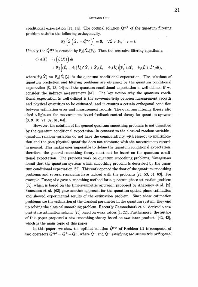
probability theory from the elementary probability theory [44, 33, 35].Consider a set of outcomes \{x_{1}, \cdots , x_{n}\} of the random variable X and an n‐
dimensional variable x=(x_{i})\in \mathbb{R}^{n} with probability vector p=(p_{i});p_{i}\geq 0, \displaystyle \sum_{i=1}^{n}p_{i}=1Then the expectation of the random variable x under probability vector p can be de‐
scribed as
\displaystyle \sum_{i=1}^{n}p_{i}x_{i}=\mathrm{T}\mathrm{r}\Vert^{p_{1_{p_{2}}}} Pn]\left\{\begin{array}{llll}x_{1} & & & \\ & x_{2} & & \\ & & \ddots & \\ & & & x_{n}\end{array}\right\}]=\mathrm{T}\mathrm{r}[\left\{\begin{array}{ll}p_{1}** & *\\*p_{2}*** & *\\***...p_{n}* & \end{array}\right\}\left\{\begin{array}{llll}x_{\mathrm{l}} & & & \\ & x_{2} & & \\ & & \ddots & \\ & & & x_{n}\end{array}\right\}]=\mathrm{T}\mathrm{n}[\hat{p}\hat{X}].
From the cychc property of the trace, Tr [\hat{p}\hat{X}]=\mathrm{T}\mathrm{r}[\hat{V}\hat{ $\rho$}\hat{V}^{*}\hat{V}\hat{X}\hat{V}^{*}] for any unitary matrix
\hat{V}\in \mathbb{C}^{n\mathrm{x}n} , so \hat{ $\rho$} and \hat{X} can be represented by Hermitian matrices. The \hat{p}\in \mathbb{C}^{n\mathrm{x}n} is an
extension of probability vector for matrices and the Hermitian matrix \hat{X}\in \mathbb{C}^{n\times n} is a
matrix‐version random variables. \hat{ $\rho$} is called a density matrix if \hat{ $\rho$}\geq 0 and \mathrm{T}x[\hat{p}]=1.In this paper, we call a Hermitian matrix a quantum random variable or a quantum
physical quantity whether it represents a real physical quantity or not. An outcome
of measurement of a quantum random variable is one of its eigenvalue with certain
probability determined by \hat{ $\rho$} and the measurement setup [33, 34, 35]. A probability
theory with Hermitian matrices and density matrices \{\hat{ $\rho$}\in \mathbb{C}^{n\times n}|\hat{p}\geq 0, \mathrm{T}x[\hat{p}]=1\} is called quantum probability theory, which describes the statistical structure and
probabilistic nature of quantum physics. We can find \mathrm{a}*‐isomorphism $\iota$ for a quantum
random variable \hat{X}=\hat{X}^{*}\in \mathbb{C}^{n\mathrm{x}n} such that $\iota$(\hat{X})=x\in \mathbb{R}^{n} , where x=(x_{i}) is a vector
which elements are eigenvalues of \hat{X} . The corresponding classical random variable
X: $\Omega$=\{1, 2, \cdots , n\}\rightarrow \mathbb{R} is defined by X(i)=x_{$\iota$'}.In general a quantum system is described by a suitably defined Hilbert space \mathcal{H}.
Any physical quantity of a quantum system is denoted by self‐adjoint operator \hat{X} on
23
AN INVITATION TO QUANTUM FILTERING AND SMOOTHING THEORY BASED ON TWO INNER PRODUCTS
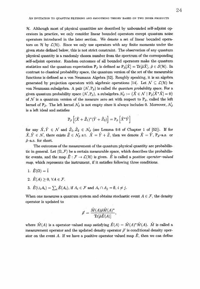
\mathcal{H} . Although most of physical quantities are described by unbounded self‐adjoint 0 $\iota$\succ
erators in practice, we only consider hnear bounded operators except quantum noise
operators introduced in the later section. We denote a set of linear bounded opera‐
tors on \mathcal{H} by \mathcal{L}(\mathcal{H}) . Since we only use operators with any finite moments under the
given state defined below, this is not strict constraint. The observation of any quantum
physical quantity is a randomly chosen number from the spectrum of the corresponding
self‐adjoint operator. Random outcomes of all bounded operators make the quantum
statistics and the quantum expectation \mathbb{P}_{\hat{ $\rho$}} is defined as \mathbb{P}_{\hat{ $\rho$}}[\hat{X}]=\ulcorner \mathrm{f}\mathrm{r}[\hat{ $\rho$}\hat{X}], \hat{ $\rho$}\in S(\mathcal{H}) . In
contrast to classical probability space, the quantum version of the set of the measurable
functions is defined as a von Neumann Algebra [52]. Roughly speaking, it is an algebra
generated by projection operators with algebraic operations [14]. Let \mathcal{N}\underline{\subseteq}\mathcal{L}(\mathcal{H}) be
von Neumann subalgebra. A pair (\mathcal{N},\mathbb{P}_{\hat{ $\rho$}}) is called the quantum probability space. For a
given quantum probability space (\mathcal{N},\mathbb{P}_{\hat{ $\rho$}}) , a subalgebra \mathcal{N}_{\hat{ $\rho$}} :=\{\hat{X}\in \mathcal{N}|\mathbb{P}_{\hat{ $\rho$}}[\hat{X}^{*}\hat{X}]=0\}of \mathcal{N} is a quantum version of the measure zero set with respect to \mathbb{P}_{\hat{ $\rho$}} , called the left
kernel of \mathbb{P}_{\overline{ $\rho$}} . The left kernel \mathcal{N}_{\hat{ $\rho$}} is not empty since it always includes O. Moreover, \mathcal{N}_{\hat{ $\rho$}}is a left ideal and satisfies
\mathbb{P}_{\hat{ $\rho$}}[(\hat{X}+\hat{Z}_{1})^{*}(\hat{Y}+\hat{Z}_{2})]=\mathbb{P}_{\hat{ $\rho$}}[\hat{X}^{*}\hat{Y}]for any \hat{X}, Y $\Lambda$\in \mathcal{N} and \hat{Z}_{1}, \hat{Z}_{2}\in \mathcal{N}_{\hat{ $\rho$}} (see Lemma 9.6 of Chapter 1 of [52]). If for
\hat{X},\hat{Y}\in \mathcal{N} , there exists \hat{Z}\in \mathcal{N}_{\hat{ $\rho$}} s.t. \hat{X}=\hat{Y}+\hat{Z} , then we denote \hat{X}=\hat{Y} , \mathbb{P}_{\hat{p}}-\mathrm{a}.\mathrm{s} . or
P‐a.s. for short.
The outcomes of the measurement of the quantum physical quantity are probabilis‐tic in general. Let ( $\Omega$,\mathcal{F}) be a certain measurable space, which describes the probabilis‐tic events, and the map Ê : \mathcal{F}\rightarrow \mathcal{L}(\mathcal{H}) is given. Ê is called a positive operator‐valued
map, which represents the instrument, if it satisfies following three conditions.
1. Ê ( $\Omega$)=\mathrm{i}
2. \^{E}(A)\geq 0, \forall A\in \mathcal{F}.
3. \displaystyle \hat{E}(\bigcup_{i}A_{i})=\sum_{i} Ê(Ai), if A_{i}\in \mathcal{F} and A_{i}\cap A_{j}=\emptyset, i\neq j.
When one measures a quantum system and obtains stochastic event A\in \mathcal{F} , the densityoperator is updated to
\displaystyle \hat{ $\rho$}=\frac{\hat{M}(A)\hat{ $\rho$}\hat{M}(A)^{*}}{\mathrm{T}\mathrm{n}[\hat{p}\^{E}(A)]},where \hat{M}(A) is a operator‐valued map satisfying \^{E}(A)=\hat{M}(A)^{*}\hat{M}(A).\hat{M} is called a
measurement operator and the updated density operator \hat{ $\rho$} is conditional density oper‐
ator on the event A . If we have a positive operator valued map Ê, then we can define
24

KENTARO OHKI
the classical probability space ( $\Omega$,\mathcal{F},\mathrm{P}) with a probability measure \mathrm{P}(A)=\mathbb{P}_{\hat{ $\rho$}}[\hat{E}(A)],for A\in \mathcal{F} . When we consider some quantum systems, algebraic tensor product Hilbert
space is used for representation of the compound quantum system. We omit this math‐
ematical definition (see, e.g., [12]).
Figure 2. Quantum‐classical correspondence
§2.2. Indirect measurement and Bayesian approach
It is difficult to observe a quantum physical quantity directly due to the mea‐
surement back actions. In this paper, we consider quantum indirect measurement to
estimate the physical quantity \hat{X} . The quantum indirect measurement is often used in
experiments and a natural setup for the quantum indirect measurement is as folows.
First, we prepare a probe system \mathcal{H}_{P} and make it interact with the system \mathcal{H}_{S} . The
interaction is represented by a suitable unitary operator Û over the compound system
\mathcal{H}_{S}\otimes \mathcal{H}_{P} . For simplicity, we consider finite dimensional Hilbert spaces, i.e., \mathcal{H}_{S}=\mathbb{C}^{n}
and \mathcal{H}_{P}=\mathbb{C}^{7n} . We measure a physical quantity of the probe system \hat{\mathrm{Y}}\in \mathcal{L}(\mathcal{H}_{P})instead of the system�s physical quantity \hat{X}\in \mathcal{L}(\mathcal{H}_{S}) . If the initial state is given by
\hat{ $\rho$}s\otimes\hat{p}_{P}\in \mathcal{S}(\mathcal{H}_{\mathcal{S}}\otimes \mathcal{H}_{P}) . After the interaction, one of eigenvalues of \hat{U}^{*}(\mathrm{i}_{S}\otimes\hat{Y})\hat{U} is
detected. Suppose the eigenvalue decomposition of \hat{Y} is \displaystyle \hat{Y}=\sum_{i=1}^{m}y_{i}\hat{P}(i) , y_{i}\neq y_{j} if
i\neq j , and y_{k} is observed. The update of the entire density matrix is
\displaystyle \hat{ $\rho$}s\otimes\hat{p}_{P}\mapsto\hat{ $\rho$}_{\mathrm{e}nt}:=\frac{\hat{U}^{*}(\hat{1}_{S}\otimes\hat{P}(k))\hat{U}(\hat{ $\rho$}s\otimes\hat{ $\rho$}_{P})\hat{U}^{*}(\hat{1}_{S}\otimes\hat{P}(k))\hat{U}}{\mathrm{T}\mathrm{r}[\hat{p}_{S}\otimes\hat{ $\rho$}_{P}\hat{U}^{*}(\hat{1}_{S}\otimes\hat{P}(k))\hat{U}]},and the conditional expectation of the physical quantity \hat{X} after the interaction is
Tr [Û* (x\hat{} \otimes \mathrm{i}_{P})\hat{U}\hat{ $\rho$}_{ent}]=\mathrm{T}\mathrm{r}[(\hat{X}\otimes \mathrm{i}_{P})\hat{U}\hat{ $\rho$}_{\mathrm{e}nt}\hat{U}^{*}]=\mathrm{T}\mathrm{r}[\hat{X}\hat{ $\rho$}_{S}],
where the posteriori density \hat{ $\rho$}_{S} is obtained by \hat{p}_{S}=\mathrm{T}\mathrm{r}_{P}[\hat{U}\hat{p}_{ent}^{\^{U}*}] and \mathrm{T}\mathrm{r}_{P} is the partialtrace operator that trace out over \mathcal{H}_{P} . The value \mathrm{T}x[\hat{X}\hat{p}_{S}] is the expectation under the
25

AN INVITATION TO QUANTUM FILTERING AND SMOOTHING THEORY BASED ON TWO INNER PRODUCTS
conditional density matrix \hat{p}_{S} , so this is the quantum conditional expectation of \hat{X}.This Bayesian approach shows the evolution of the conditional density matrix \hat{ $\rho$}s . The
update of the conditional density operator for finite dimensional descrete time quantum
systems is clear, though, it is difficult to extend to the infinite dimensional continuous
time quantum systems. We give another approach to the estimation of the quantum
physical quantity below.
§2.3. A quantum minimum mean square estimation
Let \hat{X}=\hat{X}^{*}\in \mathbb{C}^{n\times n} and a map \hat{P} : \{ 1, 2, \cdots, m\}\rightarrow \mathbb{C}^{n\times n} satisfying \hat{P}(i)=\hat{P}(i)^{*}=\hat{P}(i)^{2}, \displaystyle \sum_{i=1}^{ $\tau$ n}\hat{P}(i)=\mathrm{i} and \hat{P}(i)\hat{P}(j)=$\delta$_{ij}\hat{P}(i) , i,j=1 , 2, \cdots, m , where m\leq n,
are given. The map \hat{P} is called the projection‐valued measure or the spectral measure
in quantum probability theory or hnear operator theory. Then consider the followingminimum mean square optimization problem;
(2.1) \displaystyle \min_{\{(q_{i},p_{i})\}_{4=1}^{m}\subset \mathrm{R}^{2}}\mathbb{P}_{\hat{ $\rho$}}[|\hat{X}-\hat{Q}|^{2}], \hat{Q} :=\sum_{i=1}^{m}(q_{i}+\mathrm{i}p_{i})\hat{P}(i) .
Since
\displaystyle \mathbb{P}_{\hat{p}}[|\hat{X}-\hat{Q}|^{2}]=\sum_{i\in \mathcal{I}}\mathbb{P}_{\hat{ $\rho$}}[\hat{P}(i)](q_{i}-\frac{1}{2}\frac{\mathbb{P}_{\hat{ $\rho$}}[\hat{P}(i)\hat{X}+\hat{X}\hat{P}(i)]}{\mathbb{P}_{\hat{ $\rho$}}[\hat{P}(i)]})^{2}+\displaystyle \sum_{i\in \mathcal{I}}\mathbb{P}_{\hat{ $\rho$}}[P^{ $\Lambda$}(i)](p_{i}-\frac{1}{2\mathrm{i}}\frac{\mathbb{P}_{\hat{ $\rho$}}[\hat{P}(i)\hat{X}-\hat{X}\hat{P}(i)]}{\mathbb{P}_{\hat{ $\rho$}}[\hat{P}(i)]})^{2}+\displaystyle \mathbb{P}_{\hat{ $\rho$}}[\hat{X}^{2}]-\sum_{i\in \mathcal{I}}\frac{1}{4}\frac{\mathbb{P}_{\hat{ $\rho$}}[\hat{P}(i)\hat{X}+\hat{X}\hat{P}(i)]^{2}}{\mathbb{P}_{\hat{ $\rho$}}[\hat{P}(i)]}-\displaystyle \sum_{i\in \mathcal{I}}\frac{1}{4}\frac{|\mathbb{P}_{\hat{ $\rho$}}[\hat{P}(i)\hat{X}-\hat{X}\hat{P}(i)]|^{2}}{\mathbb{P}_{\hat{ $\rho$}}[\hat{P}(i)]},
where \mathcal{I}:=\{i=1, m|\mathrm{T}\mathrm{r}[\hat{p}\hat{P}(i)]\neq 0\} , the optimization problem (2.1) is easy to
solve and we obtain the optimal parameters
(2.2) q_{i}^{\mathrm{o}\mathrm{p}\mathrm{t}}=\displaystyle \frac{1}{2}\frac{\mathbb{P}_{\hat{ $\rho$}}[\hat{P}(i)\hat{X}+\hat{X}\hat{P}(i)]}{\mathbb{P}_{\hat{ $\rho$}}[\hat{P}(i)]}=\ulcorner \mathrm{r}_{\mathrm{r}}[\frac{\hat{ $\rho$}\hat{P}(i)+\hat{P}(i)\hat{ $\rho$}}{2\mathrm{T}\mathrm{r}[\hat{p}\hat{P}(i)]}\hat{X}], \forall i\in \mathcal{I},(2.3) p_{i}^{\mathrm{o}\mathrm{p}\mathrm{t}}=\displaystyle \frac{1}{2\mathrm{i}}\frac{\mathbb{P}_{\hat{ $\rho$}}[\hat{P}(i)\hat{X}-\hat{X}\hat{P}(i)]}{\mathbb{P}_{\hat{ $\rho$}}[\hat{P}(i)]}=-\mathrm{i}\mathrm{T}\mathrm{n}[\frac{\hat{ $\rho$}\hat{P}(i)-\hat{P}(i)\hat{p}}{2\mathrm{T}\mathrm{r}[\hat{p}\hat{P}(i)]}\hat{X}], \forall i\in \mathcal{I}.
26
KENTARO OHKI
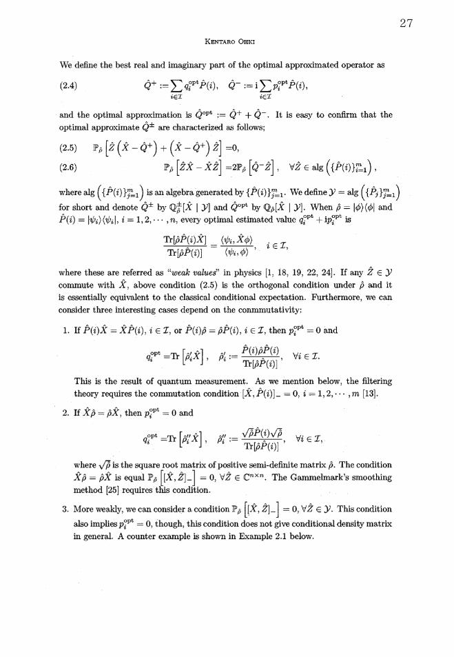
We define the best real and imaginary part of the optimal approximated operator as
(2.4) \displaystyle \hat{Q}^{+}:=\sum_{i\in \mathcal{I}}q_{i}^{\mathrm{o}\mathrm{p}\mathrm{t}}\hat{P}(i) , \hat{Q}^{-}:=\mathrm{i}\sum_{i\in \mathcal{I}}p_{i}^{\mathrm{o}\mathrm{p}\mathrm{t}}\hat{P}(i) ,
and the optimal approximation is \hat{Q}^{\mathrm{o}\mathrm{p}\mathrm{t}}:=\hat{Q}^{+}+\hat{Q}^{-} It is easy to confirm that the
optimal approximate \hat{Q}^{\pm} are characterized as follows;
(2.5) \mathbb{P}_{\hat{ $\rho$}}[\hat{Z}(\hat{X}-\hat{Q}^{+})+(\hat{X}-\hat{Q}^{+})\hat{Z}]=0,(2.6) \mathbb{P}_{\hat{ $\rho$}}[\hat{Z}\hat{X}-\hat{X}\hat{Z}]=2\mathbb{P}_{\hat{ $\rho$}}[\hat{Q}^{-}\hat{Z}], \forall\hat{Z}\in alg (\{\hat{P}(i)\}_{i=1}^{7n}) ,
where alg (\{\hat{P}(i)\}_{j=1}^{m}) is an algebra generated by \{\hat{P}(i)\}_{j=1}^{m} . We define \mathrm{y}= alg (\{\hat{P}_{j}\}_{J'}^{m}=1)for short and denote \hat{Q}^{\pm} by \mathbb{Q}_{\hat{ $\rho$}}^{\pm}[\hat{X}|\mathcal{Y}] and \hat{Q}^{\mathrm{o}\mathrm{p}\mathrm{t}} by \mathbb{Q}_{\hat{ $\rho$}}[\hat{X}|\mathcal{Y}] . When \hat{ $\rho$}=| $\phi$} \langle $\phi$| and
\hat{P}(i)=\}$\psi$_{i}\rangle\langle$\psi$_{i}|, i=1 , 2, \cdots
, n , every optimal estimated value q_{i}^{\mathrm{o}\mathrm{p}\mathrm{t}}+\mathrm{i}p_{i}^{\mathrm{o}\mathrm{p}\mathrm{t}} is
\displaystyle \frac{\mathrm{T}\mathrm{r}[\hat{ $\rho$}\hat{P}(i)\hat{X}]}{\mathrm{T}\mathrm{r}[\hat{p}\hat{P}(i)]}=\frac{\langle$\psi$_{i},\hat{X} $\phi$\}}{\langle$\psi$_{i}, $\phi$\rangle}, i\in \mathcal{I},where these are referred as �weak values� in physics [1, 18, 19, 22, 24]. If any \hat{Z}\in \mathcal{Y}commute with \hat{X} , above condition (2.5) is the orthogonal condition under \hat{p} and it
is essentially equivalent to the classical conditional expectation. Furthermore, we can
consider three interesting cases depend on the conmmutativity:
1. If \hat{P}(i)\hat{X}=\hat{X}\hat{P}(i) , i\in \mathcal{I}, or \hat{P}(i)\hat{ $\rho$}=\hat{ $\rho$}\hat{P}(i) , i\in \mathcal{I} , then p_{i}^{\mathrm{o}\mathrm{p}\mathrm{t}}=0 and
q_{i}^{\mathrm{o}\mathrm{p}\mathrm{t}}=\displaystyle \mathrm{T}\mathrm{r}[\hat{ $\rho$}_{i}\hat{X}], \hat{ $\rho$}_{i}:=\frac{\hat{P}(i)\hat{ $\rho$}\hat{P}(i)}{\mathrm{T}\mathrm{r}[\hat{ $\rho$}\hat{P}(i)]}, \forall i\in \mathcal{I}.This is the result of quantum measurement. As we mention below, the filteringtheory requires the commutation condition [\hat{X}, \hat{P}(i)]_{-}=0, i=1 , 2, \cdots, m[13].
2. If \hat{X}\hat{ $\rho$}=\hat{ $\rho$}\hat{X} , then p_{i}^{\mathrm{o}\mathrm{p}\mathrm{t}}=0 and
q_{i}^{\mathrm{o}\mathrm{p}\mathrm{t}}=\displaystyle \mathrm{T}\mathrm{r}[\hat{ $\rho$}_{i}\hat{X}], \hat{ $\rho$}_{i}^{/}:=\frac{\sqrt{\hat{ $\rho$}}\hat{P}(i)\sqrt{\hat{ $\rho$}}}{\mathrm{T}\mathrm{r}[\hat{p}\hat{P}(i)]}, \forall i\in \mathcal{I},where \sqrt{\hat{ $\rho$}} is the square root matrix of positive semi‐definite matrix \hat{ $\rho$} . The condition
\hat{X}\hat{ $\rho$}=\hat{ $\rho$}\hat{X} is equal \mathbb{P}_{\hat{ $\rho$}}[[\hat{X}, Z =0, \forall\hat{Z}\in \mathbb{C}^{n\mathrm{x}n} . The Gammelmark�s smoothingmethod [25] requires this condition.
3. More weakly, we can consider a condition \mathbb{P}_{\hat{ $\rho$}}[[\hat{X}, Z =0, \forall\hat{Z}\in \mathcal{Y} . This condition
also implies p_{i}^{\mathrm{o}\mathrm{p}\mathrm{t}}=0 , though, this condition does not give conditional density matrix
in general. A counter example is shown in Example 2.1 below.
27

AN INVITATION TO QUANTUM FILTERING AND SMOOTHING THEORY BASED ON TWO INNER PRODUCTS
Two obtained matrices \hat{p}_{i} and \hat{p}_{i} are also density operators, so the optimal approxima‐tion is given by �a conditional expectation On the other hand, the general approxima‐tion (2.2) is not able to be interpreted as the conditional expectation because \mathbb{Q}_{\hat{ $\rho$}}^{+}[\hat{X}|\mathcal{Y}]is not positive even if \hat{X} is a positive operator. For any matrix \hat{X}\in \mathbb{C}^{n\mathrm{x}n} , the following
equality holds:
\mathbb{P}_{\hat{ $\rho$}}[\hat{Z}(\hat{X}-\mathbb{Q}_{\hat{ $\rho$}}^{+}[\hat{X}|\mathcal{Y} =\displaystyle \frac{1}{2}\mathbb{P}_{\hat{ $\rho$}}[\hat{Z}\hat{X}-\hat{X}\hat{Z}]=\mathbb{P}_{\hat{ $\rho$}}[\mathbb{Q}_{\hat{ $\rho$}}^{-}[\hat{X}|y]\hat{z}], \forall\hat{Z}\in y.
Example 2.1. Consider the following density matrix, Hermitian matrix and a
set of diagonal matrices
\displaystyle \hat{ $\rho$}=\frac{1}{2}\left\{\begin{array}{l}11\\1\mathrm{l}\end{array}\right\}, \hat{X}=\left\{\begin{array}{ll}1 & 2-\mathrm{i} $\alpha$\\ 2+\mathrm{i} $\alpha$ & 3\end{array}\right\}, $\alpha$\displaystyle \in \mathbb{R}, \mathcal{Y}=\{\left\{\begin{array}{ll}a & 0\\0 & b\end{array}\right\}, a, b\displaystyle \in \mathbb{C}\}.Then,
\mathbb{Q}_{\hat{ $\rho$}}^{+}[\hat{x}|y]=\left\{\begin{array}{l}30\\05\end{array}\right\} \mathbb{Q}_{\hat{ $\rho$}}^{-}[\hat{X}|y]=\mathrm{i} $\alpha$\left\{\begin{array}{l}-10\\01\end{array}\right\}The matrix \hat{X} has a negative eigenvalue, though, the approximation \mathbb{Q}_{\hat{ $\rho$}}^{+}[\hat{X}|\mathcal{Y}] is a
positive‐definite matrix. If $\alpha$=0 , then \mathbb{P}_{\hat{ $\rho$}}[[\hat{X} , \hat{Z}]_{-}]=0, \forall\hat{Z}\in \mathcal{Y}.
If we choose the \hat{X} as a positive‐definite matrix
\hat{X}=[^{\sqrt{111}-0.1-1}-1\sqrt{111}+0.1],then
\displaystyle \mathbb{Q}_{\hat{ $\rho$}}^{+}[\hat{X}|y]=\frac{1}{2}[^{\sqrt{111}-1.10}0\sqrt{111}+1.1].This approximation has negative eigenvalue, so positive‐definiteness is not preserved in
general.
§3. Quantum conditional expectation and minimum mean square
approximation
In this section, we introduce real and imaginary parts of the best approximation in
the sense of the semi‐norms induced by the pre‐inner products below and show several
properties of them. Let y be a commutative *‐subalgebra of \mathcal{L}(\mathcal{H}) . We introduce
another *−subalgebra whose elements commute with \mathfrak{N} of the elements in \mathcal{Y} ;
\mathcal{Y} :=\{\hat{X}\in \mathcal{L}(\mathcal{H})|\hat{X}\hat{Y}=\hat{\mathrm{Y}}\hat{X}, \forall\hat{Y}\in \mathcal{Y}\}.
28

KENTARO OHKI
Hereafter we assume \mathcal{Y}=(\mathcal{Y}')' , i.e., y is a commutative von Neumann subalgebra
[13, 52]. For instance, y=\mathrm{a}\mathrm{l}\mathrm{g}(\{\hat{P}_{j}\}_{j=1}^{m}) is a commutative von Neumann subalgebraof \mathbb{C}^{n\times n} . von Neumann algebras are a generalization of the set of the $\sigma$‐measurable
bounded functions and especially a commutative von Neumann algebra is isomorphicto the set of the $\sigma$‐measurable bounded functions. Note that \mathcal{Y}' is generally non‐
commutative *‐subalgebra. Let us define the quantum conditional expectation (see,e.g., [52, Prop. 2.36] and [13, Sec. 3]) and the optimal approximation as we discussed
above.
§3.1. Definitions
We introduce three approximations of a given \hat{X}\in \mathcal{L}(\mathcal{H}) . All of them are based
on the following pre‐inner products [4].
Definition 3.1. For given \hat{p}\in \mathcal{S}(\mathcal{H}) ,
1. the pre‐inner product \langle \mathrm{e}, 0\rangle_{\hat{ $\rho$}} : \mathcal{L}(\mathcal{H})\times \mathcal{L}(\mathcal{H})\rightarrow \mathbb{C} is defined by \{\hat{X}, \hat{Y}\rangle_{\hat{ $\rho$}} :=\mathbb{P}_{\hat{ $\rho$}}[\hat{X}^{*}\hat{Y}].2. the symmetric pre‐inner product \langle\langle, \rangle\rangle_{\hat{ $\rho$}} : \mathcal{L}(\mathcal{H})\times \mathcal{L}(\mathcal{H})\rightarrow \mathbb{C} is defined by
\{\langle\hat{X}, \hat{Y}\rangle\rangle_{\hat{p}} :=\displaystyle \frac{1}{2}\mathbb{P}_{\hat{ $\rho$}}[\hat{X}^{*}\hat{Y}+\hat{Y}\hat{X}^{*}].Note that \langle\langle\hat{X}, \hat{Y} } )_{\hat{ $\rho$}} is not a real part of \langle\hat{X}, \hat{Y}\rangle_{\hat{ $\rho$}} . The pre‐inner product \langle\langle, } \rangle_{\hat{ $\rho$}}
is also used in quantum infromation geometry [4]. These pre‐inner products satisfy the
Cauchy‐Schwarz inequality (see, e.g., Proposition 9.5 of [52]). \langle\hat{X}, \hat{X}\}_{\hat{ $\rho$}}=0 is necessary
and sufficient condition for \hat{X}\in \mathcal{N}_{\hat{ $\rho$}} , though, \langle\{\hat{X}, \hat{X}\rangle\rangle_{\hat{ $\rho$}}=0 is not. If \hat{X}\in \mathcal{N}_{\hat{p}}\cap \mathcal{Y},then \langleX, \hat{X}\}_{\hat{ $\rho$}}=\{\langle\hat{X}, \hat{X}\rangle\}_{\hat{ $\rho$}}=0 . This is proven by the Cauchy‐Schwarz inequality and
commutativity of \mathcal{Y} . We use two measures to find the best approximation in \mathcal{Y} , where
the �probability zero� space is common whenever any of two semi‐inner products is
used.
Definition 3.2 (Quantum conditional expectation).Let (\mathcal{L}(\mathcal{H}), \mathbb{P}_{\hat{ $\rho$}}) be a quantum probability space and y be a commutative von Neu‐
mann sub‐algebra of \mathcal{L}(\mathcal{H}) . A linear operator \hat{Q}\in y is called a version of the quantumconditional expectation if there exists \hat{Q}\in \mathcal{Y} satisfies
(3.1) \langle\hat{Z}, \hat{X}-\hat{Q}\rangle_{\hat{ $\rho$}}=0, \forall\hat{Z}\in y
for arbitrary fixed \hat{X}\in \mathcal{Y} . Then we denote \hat{Q}=\mathbb{P}_{\hat{ $\rho$}}[\hat{X}|\mathcal{Y}].Some properties of the quantum conditional expectation are shown in, for ex‐
\hat{X}\partial-\mathbb{P}_{\hat{ $\rho$}}\mathrm{t}^{13].\mathrm{J}\mathrm{e}\mathrm{x}\mathrm{p}\mathrm{e}\mathrm{c}\mathrm{t}\mathrm{a}\mathrm{t}\mathrm{i}\mathrm{o}\mathrm{n}\mathrm{i}\mathrm{m}\mathrm{p}1\mathrm{i}\mathrm{e}\mathrm{s}\mathrm{t}\mathrm{h}\mathrm{a}\mathrm{t}\mathrm{t}\mathrm{h}\mathrm{e}}\hat{X}|\mathcal{Y}]\mathrm{a}\mathrm{n}\mathrm{d}\mathrm{t}1_{2}\mathrm{e}\mathrm{c}ommutative s \mathrm{u}\mathrm{k}\mathrm{a}1gebra \mathcal{Y}\mathrm{a}\mathrm{r}\mathrm{e}\mathrm{o}\mathrm{r}\mathrm{t}\mathrm{h}\mathrm{o}\mathrm{g}\mathrm{o}\mathrm{n}\mathrm{a}1 under t \mathrm{h}\mathrm{e}\mathrm{s}tate\mathbb{P}_{\hat{ $\rho$}}\mathrm{T}\mathrm{h}\mathrm{e}\mathrm{d}\mathrm{e}\mathrm{f}\mathrm{i}\dot{\mathrm{m}}tion o \mathrm{f}\mathrm{t}\mathrm{h}\mathrm{e}\mathrm{q}uantum c \mathrm{o}\mathrm{n}\mathrm{d}\mathrm{i}\mathrm{t}\mathrm{i}\mathrm{o}\mathrm{n}\partial
We extend the definition of orthogonality to non‐commutative regime.
29
AN INVITATION TO QUANTUM FILTERING AND SMOOTHING THEORY BASED ON TWO INNER PRODUCTS
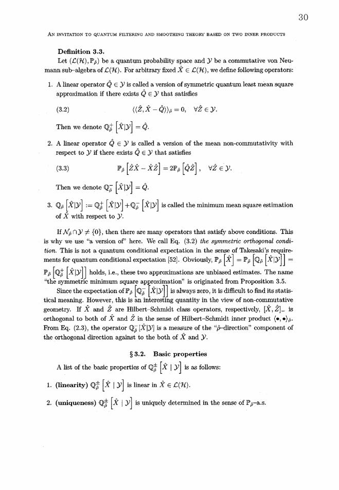
Definition 3.3.
Let (\mathcal{L}(\mathcal{H}), \mathbb{P}_{\hat{ $\rho$}}) be a quantum probability space and \mathcal{Y} be a commutative von Neu‐
mann sub‐algebra of \mathcal{L}(\mathcal{H}) . For arbitra1y fixed \hat{X}\in \mathcal{L}(\mathcal{H}) , we define following operators:
1. A linear operator \hat{Q}\in \mathcal{Y} is caned a version of symmetric quantum least mean square
approximation if there exists \hat{Q}\in \mathcal{Y} that satisfies
(3.2) \{\langle\hat{Z},\hat{X}-\hat{Q}\}\rangle_{\hat{ $\rho$}}=0, \forall\hat{Z}\in \mathcal{Y}.
Then we denote \mathbb{Q}_{\hat{ $\rho$}}^{+}[\hat{X}|\mathcal{Y}]=\hat{Q}.2. A linear operator \hat{Q}\in y is called a version of the mean non‐commutativity with
respect to \mathcal{Y} if there exists \hat{Q}\in y that satisfies
(3.3) \mathbb{P}_{\hat{ $\rho$}}[\hat{Z}\hat{X}-\hat{X}\hat{Z}]=2\mathbb{P}_{\hat{ $\rho$}}[\hat{Q}\hat{Z}], \forall\hat{Z}\in y.
Then we denote \mathbb{Q}_{\hat{ $\rho$}}^{-}[\hat{X}|\mathcal{Y}]=\hat{Q}.3. \mathbb{Q}_{\hat{ $\rho$}}[\hat{X}|y]\wedge :=\mathbb{Q}_{\hat{ $\rho$}}^{+}[\hat{X}|\mathcal{Y}]+\mathbb{Q}_{\hat{ $\rho$}}^{-}[\hat{x}|y] is called the minimum mean square estimation
of X with respect to \mathcal{Y}.
If \mathcal{N}_{\hat{ $\rho$}}\cap \mathcal{Y}\neq\{0\} , then there are many operators that satisfy above conditions. This
is why we use �a version of� here. We call Eq. (3.2) the symmetric orthogonal condi‐
tion. This is not a quantum conditional expectation in the sense of Takesaki�s require‐ments for quantum conditional expectation [52]. Obviously, \mathbb{P}_{\hat{p}}[\hat{X}]=\mathbb{P}_{\hat{ $\rho$}}[\mathbb{Q}_{\hat{ $\rho$}}[\hat{X}|\mathcal{Y}]]=\mathbb{P}_{\hat{ $\rho$}}[\mathbb{Q}_{\hat{ $\rho$}}^{+}[\hat{X}|y]] holds, i.e., these two approximations are unbiased estimates. The name
�the symmetric minimum square approximation�� is originated from Proposition 3.5.
Since the expectation of \mathbb{P}_{\hat{ $\rho$}}[\mathbb{Q}_{\hat{ $\rho$}}^{-}[\hat{X}|y]] is always zero, it is difficult to find its statis‐
tical meaning. However, this is an interesting quantity in the view of non‐commutative
geometry. If \hat{X} and \hat{Z} are Hilbert‐Schmidt class operators, respectively, [\hat{X}, Z is
orthogonal to both of \hat{X} and \hat{Z} in the sense of Hilbert‐Schmidt inmer product \langle, \rangle_{\hat{ $\rho$}}.Fkom Eq. (2.3), the operator \mathbb{Q}_{\hat{ $\rho$}}^{-}[\hat{X}|\mathcal{Y}] is a measure of the \hat{p}−-ddirection component of
the orthogonal direction against to the both of \hat{X} and y.
§ S. 2. Basic properties
A list of the basic properties of \mathbb{Q}_{\hat{ $\rho$}}^{\pm}[\hat{X}|\mathcal{Y}] is as follows:
1. (linearity) \mathbb{Q}_{\hat{ $\rho$}}^{\pm}[\hat{X}|\mathcal{Y}] is linear in \hat{X}\in \mathcal{L}(\mathcal{H}) .
2. (uniqueness) \mathbb{Q}_{\hat{ $\rho$}}^{\pm}[\hat{X}|\mathcal{Y}] is uniquely determined in the sense of \mathbb{P}_{\hat{ $\rho$}}-\mathrm{a}.\mathrm{s}.
30
KENTARO OHKI
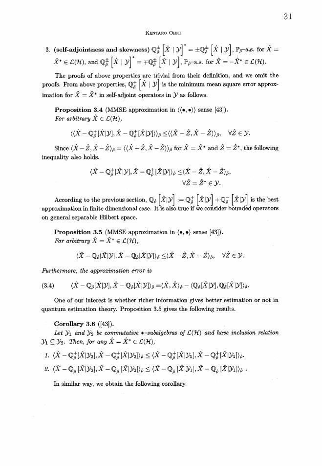
3. (self‐adjointness and skewness) \mathbb{Q}_{\hat{ $\rho$}}^{\pm}[\hat{X}|\mathcal{Y}]^{*}=\pm \mathbb{Q}_{\hat{ $\rho$}}^{\pm}[\hat{X}|\mathcal{Y}], \mathbb{P}_{\hat{ $\rho$}}-\mathrm{a}.\mathrm{s} . for \hat{X}=
\hat{X}^{*}\in \mathcal{L}(\mathcal{H}) , and \mathbb{Q}_{\hat{ $\rho$}}^{\pm}[\hat{X}|\mathcal{Y}]^{*}=\mp \mathbb{Q}_{\hat{ $\rho$}}^{\pm}[\hat{X}|\mathcal{Y}], \mathbb{P}_{\hat{ $\rho$}}-\mathrm{a}.\mathrm{s} . for \hat{X}=-\hat{X}^{*}\in \mathcal{L}(\mathcal{H}) .
The proofs of above properties are trivial from their definition, and we omit the
proofs. From above properties, \mathbb{Q}_{\hat{ $\rho$}}^{+}[\hat{X}|\mathcal{Y}] is the minimum mean square error approx‐
imation for \hat{X}=\hat{X}^{*} in self‐adjoint operators in \mathcal{Y} as follows.
Proposition 3.4 (MMSE approximation in \langle\langle, \rangle\rangle sense [43]).For arbitrary \hat{X}\in \mathcal{L}(\mathcal{H})_{f}
\{\langle\hat{X}-\mathbb{Q}_{\hat{ $\rho$}}^{+}[\hat{X}|\mathcal{Y}],\hat{X}-\mathbb{Q}_{\hat{ $\rho$}}^{+}[\hat{X}|\mathcal{Y}]\}\rangle_{\hat{ $\rho$}}\leq\{\{\hat{X}-\hat{Z}, \hat{X}-\hat{Z})\rangle_{\hat{ $\rho$}}, \forall\hat{Z}\in y.Since \langle X-\hat{Z},\hat{X}-\hat{Z}\}_{\hat{ $\rho$}}=\{\langle\hat{X}-\hat{Z} , \hat{X}-\hat{Z}\rangle\rangle_{\hat{ $\rho$}} for \hat{X}=\hat{X}^{*} and \hat{Z}=\hat{Z}^{*} , the following
inequality also holds.
\langle\hat{X}-\mathbb{Q}_{\hat{ $\rho$}}^{+}[\hat{X}|\mathcal{Y}],\hat{X}-\mathbb{Q}_{\hat{ $\rho$}}^{+}[\hat{X}|\mathcal{Y}]\}_{\hat{ $\rho$}}\leq\{\hat{X}-\hat{Z},\hat{X}-\hat{Z}\rangle_{\hat{ $\rho$}},\forall\hat{Z}=\hat{Z}^{*}\in \mathcal{Y}.
According to the previous section, \mathbb{Q}_{\hat{ $\rho$}}[\hat{X}|y] :=\mathbb{Q}_{\hat{ $\rho$}}^{+}[\hat{X}|\mathcal{Y}]+\mathbb{Q}_{\hat{ $\rho$}}^{-}[\hat{X}|\mathrm{y}] is the best
approximation in finite dimensional case. It is also true if we consider bounded operators
on general separable Hilbert space.
Proposition 3.5 (MMSE approximation in \langle, \rangle sense [43]).For arbitrary \hat{X}=\hat{X}^{*}\in \mathcal{L}(\mathcal{H}) ,
\langle\hat{X}-\mathbb{Q}_{\hat{ $\rho$}}[\hat{X}|\mathcal{Y}],\hat{X}-\mathbb{Q}_{\hat{ $\rho$}}[\hat{X}|\mathcal{Y}]\rangle_{\hat{ $\rho$}}\leq\langle\hat{X}-\hat{Z},\hat{X}-\hat{Z}\rangle_{\hat{ $\rho$}}, \forall\hat{Z}\in y.
Furthermore, the approximation error is
(3.4) \langle\hat{X}-\mathbb{Q}_{\hat{ $\rho$}}[\hat{X}|\mathcal{Y}], \hat{X}-\mathbb{Q}_{\hat{ $\rho$}}[\hat{X}|\mathcal{Y}]\rangle_{\hat{ $\rho$}}=\langle\hat{X}, \hat{X}\rangle_{\hat{ $\rho$}}-\langle \mathbb{Q}_{\hat{ $\rho$}}[\hat{X}|\mathcal{Y}],\mathbb{Q}_{\hat{ $\rho$}}[\hat{X}|\mathcal{Y}]\rangle_{\hat{p}}.
One of our interest is whether richer information gives better estimation or not in
quantum estimation theory. Proposition 3.5 gives the following results.
Corollary 3.6 ([43]).Let y_{1} and y_{2} be commutative * ‐subalgebras of \mathcal{L}(\mathcal{H}) and have inclusion relation
\mathcal{Y}_{1}\subseteq y_{2} . Then, for any \hat{X}=\hat{X}^{*}\in L(\mathcal{H}) ,
1. \langle\hat{X}-\mathbb{Q}_{\hat{ $\rho$}}^{+}[\hat{X}|y_{2}],\hat{X}-\mathbb{Q}_{\hat{ $\rho$}}^{+}[\hat{X}|\mathcal{Y}_{2}]\rangle_{\hat{ $\rho$}}\leq\{\hat{X}-\mathbb{Q}_{\hat{ $\rho$}}^{+}[\hat{X}|\mathcal{Y}_{\mathrm{i}}|, \hat{X}-\mathbb{Q}_{\hat{p}}^{+}[\hat{X}|\mathcal{Y}_{1}]\rangle_{\hat{ $\rho$}}.2. \langle\hat{X}-\mathbb{Q}_{\hat{p}}^{-}[\hat{X}|\mathcal{Y}_{2}],\hat{X}-\mathbb{Q}_{\hat{ $\rho$}}^{-}[\hat{X}|\mathcal{Y}_{2}]\rangle_{\hat{ $\rho$}}\leq\langle\hat{X}-\mathbb{Q}_{\hat{ $\rho$}}^{-}[\hat{X}|\mathcal{Y}_{1}],\hat{X}-\mathbb{Q}_{\hat{ $\rho$}}^{-}[\hat{X}|\mathcal{Y}_{1}]\rangle_{\hat{ $\rho$}}
In similar way, we obtain the following corollary.
31

AN INVITATION TO QUANTUM FILTERING AND SMOOTHING THEORY BASED ON TWO INNER PRODUCTS
Corollary 3.7. Let y_{1} and y_{2} be commutative * ‐subalgebras of \mathcal{L}(\mathcal{H}) and have
indusion oelation y_{1}\subseteq y_{2} . Then, for any \hat{X}=\hat{X}^{*}\in \mathcal{L}(\mathcal{H}) ,
\langle\hat{X}-\mathbb{Q}_{\hat{ $\rho$}}[\hat{X}|\mathcal{Y}_{2}], \hat{X}-\mathbb{Q}_{\hat{ $\rho$}}[\hat{X}|\mathcal{Y}_{2}]\}_{\hat{ $\rho$}}\leq\langle\hat{X}-\mathbb{Q}_{\hat{ $\rho$}}[\hat{X}|\mathcal{Y}_{1}],\hat{X}-\mathbb{Q}_{\hat{ $\rho$}}[\hat{X}|\mathcal{Y}_{1}]\rangle_{\hat{ $\rho$}}.
§3.3. Some lower bounds and remarks
To estimate the approximation error bound is important for accuracy. Roles of
the \mathbb{Q}_{\hat{ $\rho$}}^{-}[\hat{X}|\mathcal{Y}] is still unclear for the author, though, it provides a lower bound of real
MMSE and is used in the quantum smoothing equation introduced below. The following
proposition holds.
Proposition 3.8 (A lower bound of MMSE).For \hat{X}=\hat{X}^{*}\in \mathcal{L}(\mathcal{H}) ,
(3.5) \mathbb{P}_{\hat{ $\rho$}}[(\hat{X}-\mathbb{Q}_{\hat{ $\rho$}}^{+}[\hat{X}|\mathcal{Y}])^{2}]\geq \mathbb{P}_{\hat{ $\rho$}}[|\mathbb{Q}_{\hat{ $\rho$}}^{-}[\hat{X}|y]|^{2}],where  | 2 := Â*Â.
Proof. From the definitions,
\{\hat{Z}, \hat{X}-\mathbb{Q}_{\hat{ $\rho$}}^{+}[\hat{X}|\mathcal{Y}])_{\hat{ $\rho$}}=\langle\hat{Z},\mathbb{Q}_{\hat{ $\rho$}}^{-}[\hat{X}|\mathcal{Y}]\rangle_{\hat{ $\rho$}}, \forall\hat{Z}\in yholds. Since \mathbb{Q}_{\hat{ $\rho$}}^{-}[\hat{X}|\mathcal{Y}]\in \mathcal{Y} , we choose \hat{Z}=\mathbb{Q}_{\hat{ $\rho$}}^{-}[\hat{X}|\mathcal{Y}] and then
\langle \mathbb{Q}_{\hat{ $\rho$}}^{-}[\hat{X}|\mathcal{Y}],\hat{X}-\mathbb{Q}_{\hat{ $\rho$}}^{+}[\hat{X}|\mathcal{Y}]\rangle_{\hat{ $\rho$}}=\langle \mathbb{Q}_{\hat{p}}^{-}[\hat{X}|\mathcal{Y}], \mathbb{Q}_{\hat{ $\rho$}}^{-}[\hat{X}|\mathcal{Y}]\rangle_{\hat{ $\rho$}}\geq 0.
Using Schwarz�s inequality, we obtain
\{\mathbb{Q}_{\hat{ $\rho$}}^{-}[\hat{X}|\mathcal{Y}], \hat{X}-\mathbb{Q}_{\hat{ $\rho$}}^{+}[\hat{X}|\mathcal{Y}]\rangle_{\hat{ $\rho$}}\leq\sqrt{\mathbb{P}_{\hat{ $\rho$}}[|\mathbb{Q}_{\hat{ $\rho$}}^{-}[\hat{X}|\mathcal{Y}]|^{2}]\mathbb{P}_{\hat{ $\rho$}}[(\hat{X}-\mathbb{Q}_{\hat{ $\rho$}}^{+}[\hat{X}|\mathcal{Y}])^{2}]}and the inequality (3.5) holds.
\square
For example, consider the MMSE of Example 2.1. In this case, the following equal‐
ity holds;
\mathbb{P}_{\hat{ $\rho$}}[(\hat{X}-\mathbb{Q}_{\hat{ $\rho$}}^{+}[\hat{X}|\mathcal{Y}])^{2}]=$\alpha$^{2}=\mathbb{P}_{\hat{ $\rho$}}[|\mathbb{Q}_{\hat{ $\rho$}}^{-}[\hat{X}|y]|^{2}].Here, \mathbb{Q}_{\hat{ $\rho$}}^{-}[\hat{X}|\mathcal{Y}] is a measure of non‐commutativity in estimation and $\alpha$ is magnitude of
non‐commutativity between \hat{X} and y under the given state \mathbb{P}_{\hat{ $\rho$}}.
32
KENTARO OHKI
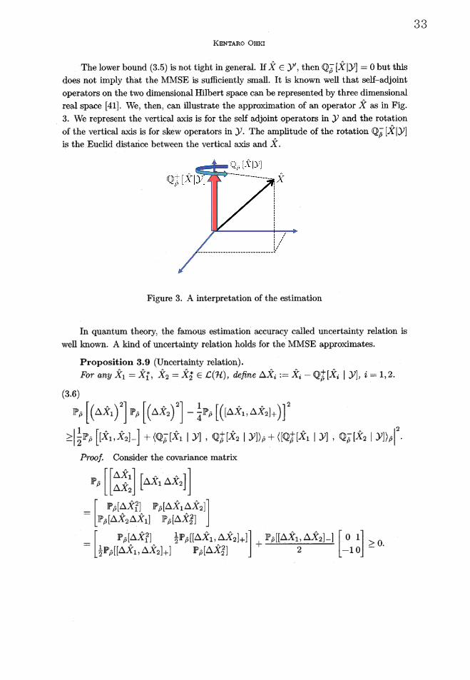
The lower bound (3.5) is not tight in general. If \hat{X}\in y , then \mathbb{Q}_{\hat{p}}^{-}[\hat{X}|y]=0 but this
does not imply that the MMSE is sufficiently small. It is known well that self‐adjoint
operators on the two dimensional Hilbert space can be represented by three dimensional
real space [41]. We, then, can illustrate the approximation of an operator \hat{X} as in Fig.3. We represent the vertical axis is for the self adjoint operators in \mathcal{Y} and the rotation
of the vertical axis is for skew operators in \mathcal{Y} . The amplitude of the rotation \mathbb{Q}_{\hat{ $\rho$}}^{-}[\hat{X}|\mathcal{Y}]is the Euclid distance between the vertical axis and \hat{X}.
Figure 3. A interpretation of the estimation
In quantum theory, the famous estimation accuracy called uncertainty relation is
well known. A kind of uncertainty relation holds for the MMSE approximates.
Proposition 3.9 (Uncertainty relation).For any \hat{X}_{1}=\hat{X}_{1}^{*}, \hat{X}_{2}=\hat{X}_{2}^{*}\in \mathcal{L}(\mathcal{H}) , define \triangle\hat{X}_{i} :=\hat{X}_{i}-\mathbb{Q}_{ $\beta$}^{+}[\hat{X}_{i}|\mathcal{Y}], i=1 ,
2.
(3.6)
\displaystyle \mathbb{P}_{\hat{p}}[(\triangle\hat{X}_{1})^{2}]\mathbb{P}_{\hat{ $\rho$}}[(\triangle\hat{X}_{2})^{2}]-\frac{1}{4}\mathbb{P}_{\hat{ $\rho$}}[([ $\Delta$\hat{X}_{1}, \triangle\hat{X}_{2}]_{+})]^{2}\displaystyle \geq|\frac{1}{2}\mathbb{P}_{\hat{ $\rho$}}[[\hat{X}_{1},\hat{X}_{2}]_{-}]+\langle \mathbb{Q}_{\hat{ $\rho$}}^{-}[\hat{X}_{1}|\mathcal{Y}], \mathbb{Q}_{\hat{ $\rho$}}^{+}[\hat{X}_{2}|\mathcal{Y}]\rangle_{\hat{ $\rho$}}+\langle[\mathbb{Q}_{\hat{ $\rho$}}^{+}[\hat{X}_{1}|\mathcal{Y}], \mathbb{Q}_{\hat{ $\rho$}}^{-}[\hat{X}_{2}|\mathcal{Y}]\}_{\hat{ $\rho$}}|^{2}
Proof. Consider the covariance matrix
\mathbb{P}_{\hat{ $\rho$}}[\left\{\begin{array}{l}\triangle\hat{X}_{1}\\\triangle\hat{X}_{2}\end{array}\right\}[ $\Delta$\hat{X}_{1}\triangle\hat{X}_{2}]]=\left\{\begin{array}{ll}\mathbb{P}_{\hat{p}}[\triangle\hat{X}_{1}^{2}] & \mathbb{P}_{\hat{p}}[\triangle\hat{X}_{1}\triangle\hat{X}_{2}]\\\mathbb{P}_{\hat{ $\rho$}}[\triangle\hat{X}_{2}\triangle\hat{X}_{1}] & \mathbb{P}_{\hat{ $\rho$}}[\triangle\hat{X}_{2}^{2}]\end{array}\right\}=[_{\frac{1}{2}\mathbb{P}_{\hat{ $\rho$}}[[\triangle\hat{X}_{1},\triangle\hat{X}_{2}]_{+}]\mathbb{P}_{\hat{ $\rho$}}[ $\Delta$\hat{X}_{2}^{2}]}\displaystyle \mathbb{P}_{\hat{ $\rho$}}[\triangle\hat{X}_{1}^{2}]\frac{1}{2}\mathbb{P}_{\hat{ $\rho$}}[[\triangle\hat{X}_{1},\triangle\hat{X}_{2}]_{+}]]+\frac{\mathbb{P}_{\hat{ $\rho$}}[[ $\Delta$\hat{X}_{1},\triangle\hat{X}_{2}]_{-}]}{2}\left\{\begin{array}{ll}0 & 1\\-10 & \end{array}\right\}\displaystyle \geq 0.
33
AN INVITATION TO QUANTUM FILTERING AND SMOOTHING THEORY BASED ON TWO INNER PRODUCTS
The determinant of the semi‐positive definite matrix is non‐negative. The straightcalculation gives
\displaystyle \mathbb{P}_{\hat{ $\rho$}}[\triangle\hat{X}_{1}^{2}]\mathbb{P}_{\hat{ $\rho$}}[ $\Delta$\hat{X}_{2}^{2}]-\frac{1}{4}\mathbb{P}_{\hat{ $\rho$}}[[\triangle\hat{X}_{1}, \triangle\hat{X}_{2}]_{+}]^{2}+\frac{1}{4}\mathbb{P}_{\hat{ $\rho$}}[[\triangle\hat{X}_{1}, \triangle\hat{X}_{2}]_{-}]^{2}\geq 0Since
\displaystyle \frac{1}{2}\mathbb{P}_{\hat{ $\rho$}}[[\triangle\hat{X}_{1}, \triangle\hat{X}_{2}]_{-}]=\frac{1}{2}\mathbb{P}_{\hat{ $\rho$}}[[\hat{X}_{1},\hat{X}_{2}]_{-}]-\mathbb{P}_{\hat{ $\rho$}}[\mathbb{Q}_{\hat{ $\rho$}}^{-}[\hat{X}_{1}|\mathcal{Y}]\mathbb{Q}_{\hat{ $\rho$}}^{+}[\hat{X}_{2}|\mathcal{Y}]]+\mathbb{P}_{\hat{p}}[\mathbb{Q}_{\hat{ $\rho$}}^{+}[\hat{X}_{1}|\mathcal{Y}]\mathbb{Q}_{\hat{ $\rho$}}^{-}[\hat{X}_{2}|\mathcal{Y}]]
=\displaystyle \frac{1}{2}\mathbb{P}_{\hat{ $\rho$}}[[\hat{X}_{1}, \hat{X}_{2}]_{-}]+\{\mathbb{Q}_{\hat{ $\rho$}}^{-}[\hat{X}_{1}|\mathcal{Y}], \mathbb{Q}_{\hat{ $\rho$}}^{+}[\hat{X}_{2}|\mathcal{Y}]\}_{\hat{ $\rho$}}+\langle[\mathbb{Q}_{\hat{ $\rho$}}^{+}[\hat{X}_{1}|\mathcal{Y}], \mathbb{Q}_{\hat{ $\rho$}}^{-}[\hat{X}_{2}|\mathcal{Y}]\rangle_{\hat{ $\rho$}}
and \mathbb{P}_{\hat{ $\rho$}}[[\triangle\hat{X}_{1} , \triangle\hat{X}_{2}]_{-}]^{2}=-|\mathbb{P}_{\hat{ $\rho$}}[[\triangle\hat{X}_{1}, \triangle\hat{X}_{2}]_{-}]|^{2} , the inequahty (3.6) holds.
\square
The inequality (3.6) is a generalization of the Schrödinger‐Robertson type uncer‐
tainty relation [35]. From the view of quantum estimation theory [59], the uncertainty
principle gives a physical estimation accuracy bound. When \mathbb{Q}_{\hat{ $\rho$}}^{-}[\hat{X}_{i}|\mathcal{Y}]=0, i=1 , 2,the inequality (3.6) is same as the Schrödinger‐Robertson type uncertainty relation. If
we want to beat the Schrödinger‐RoUertson type uncertainty relation of physical quan‐
tities \hat{X}_{1} and \hat{X}_{2} , we should choose the measurement algebra \mathcal{Y} to avoid the condition
\mathbb{Q}_{\hat{ $\rho$}}^{-}[\hat{X}_{i}|y]=0, i=1,2 simultaneously.
Remark.
The real minimum mean square approximate of \hat{X}\in \mathcal{L}(\mathcal{H}) does not satisfy the
orthogonality condition (3.1). From the definition ofthe minimum square approximation
(3.2), the �normal� orthogonal relation becomes
\mathbb{P}_{\hat{ $\rho$}}[\hat{Z}(\hat{X}-\mathbb{Q}_{\hat{ $\rho$}}^{+}[\hat{X}|\mathcal{Y}])]=\mathbb{P}_{\overline{ $\rho$}}[\mathbb{Q}_{\hat{ $\rho$}}^{-}[\hat{X}|\mathcal{Y}]\hat{Z}], \forall\hat{Z}\in \mathcal{Y}.Obviously, the estimation error \hat{X}-\mathbb{Q}_{\hat{ $\rho$}}^{+}[\hat{X}|\mathcal{Y}]\in \mathcal{L}(\mathcal{H}) is orthogonal to y if and only if
\mathbb{Q}_{\hat{ $\rho$}}^{-}[\hat{X}|\mathrm{y}]=0 under \mathbb{P}_{\hat{ $\rho$}}.\hat{X}\in y is a sufficient condition for the orthogonality condition
(3.1).
Remark.
\mathbb{P}_{\hat{ $\rho$}}[|\mathcal{Y}] , and \mathbb{Q}_{\hat{ $\rho$}}^{\pm}[|\mathcal{Y}] are regarded as a linear functional on their domains because
any commutative *‐subalgebra can be seemed as measurable functions on a suitable
chosen measurable space ( $\Omega$, \mathcal{F}) . There exists \mathrm{a}*‐isomorphism $\iota$ between \mathcal{Y} and L^{\infty}( $\Omega$) .
34

KENTARO OHKI
§4. Model and quantum filtering
§4.1. Model
Any quantum system is described by suitable Hilbert space and linear operators
on the Hilbert space. We consider two quantum systems, system and probe system.We describe them \mathcal{H}_{S} and \mathcal{H}_{P} , respectively. \mathcal{H}_{P} is a continuous Fock space [27];
\mathcal{H}_{P}=\otimes_{t\in[0,\infty)}\mathcal{H}_{P}(t) The compound quantum system is the tensor product Hilbert
space \mathcal{H}=\mathcal{H}s\otimes \mathcal{H}_{P} equipped with a density operator \hat{ $\rho$}=\hat{ $\rho$}s\otimes\hat{p}_{P}, \hat{p}s\in \mathcal{S}(\mathcal{H}_{S}) , \hat{ $\rho$}_{P}\in
\mathcal{S}(\mathcal{H}_{P}) . Physical quantities of the system are described by self adjoint operators in
\mathcal{L}(\mathcal{H}_{S}) and physical quantities of the probe system are described by self‐adjoint op‐
erators in \mathcal{L}(\mathcal{H}_{P}) . They act on the total quantum system with corresponding identity
operator, though, we omit identity operator for simplicity; \hat{x}\otimes \mathrm{i}_{P}\equiv\hat{X} and \mathrm{i}_{S}\otimes\hat{Y}\equiv\hat{Y}for \hat{X}\in \mathcal{L}(\mathcal{H}_{S}) and \hat{Y}\in \mathcal{L}(\mathcal{H}_{P}) .
)
Figure 4. Schematic diagram
In order to quantum theory, the time evolution of every physical quantity \hat{X}=\hat{X}^{*}\in
\mathcal{L}\langle \mathcal{H}) driven Uy probe system is determined by a unitary operator \hat{U}_{t} that describes the
interaction between the system and the probe. We consider the unitary operator \hat{U}_{t} as
the solution of the following equation;
(4.1) \displaystyle \frac{d}{dt}\hat{U}_{t}=(-\mathrm{i}\hat{H}+\hat{L}\hat{a}_{t}^{*} ‐ L\hat{}* ât) Ût , \^{U}_{0}=\mathrm{i}
where ât \in \mathcal{L} ( \mathcal{H}p(t)) is called the quantum white noise which satisfies
[\hat{a}_{t}, \hat{a}_{s}^{*}]_{-}= $\delta$(t-s)\mathrm{i},
where $\delta$ is Dirac�s delta function. The formal integral of the quantum white noise and
its infinitesimal increment are defined
\displaystyle \hat{A}_{t}:=\int_{0}^{t}\hat{a}_{s}ds, d\hat{A}_{t}=\hat{A}(t+dt)-\hat{A}(t) ,
35

AN INVITATION TO QUANTUM FILTERING AND SMOOTHING THEORY BASED ON TWO INNER PRODUCTS
respectively [26]. In order to quantum stochastic calculus [36], the quantum Ito�s rule
is
(4.2) \left\{\begin{array}{l}d\hat{A}_{t}d\hat{A}_{t}=d\hat{A}_{t}^{*}d\hat{A}_{t}= d\^{A} tdt=(dt)2 =0,\\d\hat{A}_{t}d\hat{A}_{t}^{*}=dt\end{array}\right.From Wong‐Zakai�s theorem, the formal equation (4.1) is described by the Hudson‐
Parthasarathy equation
(4.3) d\displaystyle \hat{U}_{t}=(-\mathrm{i}\hat{H}dt-\frac{1}{2}\hat{L}^{*}\hat{L}dt+\hat{L}d\hat{A}_{t}^{*}-\hat{L}^{*}d\hat{A}_{t})\hat{U}_{t}.Then the time evolution of the \hat{X}_{t}=\hat{U}_{t}^{*}\hat{X}\hat{U}_{t} follows the quantum stochastic differential
equation
d\displaystyle \hat{X}_{t}=\mathrm{i}[\hat{H}_{t},\hat{X}_{t}]_{-}dt+\frac{1}{2}(\hat{L}_{t}^{*}[\hat{X}_{t},\hat{L}_{t}]_{-}+[\hat{L}_{t}^{*},\hat{X}_{t}]_{-}\hat{L}_{t})dt(4.4) +[\hat{L}_{t}^{*}, \hat{X}_{t}]_{-}d\hat{A}_{t}+[\hat{X}_{t}, \hat{L}_{t}] ‐dÂt* ,
where H. =\hat{U}_{t}^{*}\hat{H}\hat{U}_{t}, \hat{L}_{t}=\hat{U}_{t}^{*}\hat{L}\hat{U}_{t} , and [Â, B :=\^{A} B\hat{} —B\hat{}
Â. For derivation, see
[13, 16, 26, 61].We consider the balanced homodyne detection as a detection of the probe system.
Its POVM is introduced in [7] and the dynamical representation is in, for example,
[26, 58]. The measurement outcome is \hat{Y}_{t}=\hat{U}_{t}^{*}(\hat{A}_{t}+\hat{A}_{\mathrm{t}}^{*})\hat{U}_{t} and its increment is
(4.5) d\hat{Y}_{t}=(\hat{L}_{t}+\hat{L}_{t}^{*})dt+d\^{A}_{t}+d\hat{A}_{t}^{*}.We define the following *−algebra by double commutant of the measurement records;
\mathcal{Y}_{t}:=(\{\hat{Y}_{s};0\leq s\leq t\})From the definitions of the unitary operator and the observed process, following
equations hold.
(4.6) \hat{X}_{t}\hat{Y}_{s}=\hat{Y}_{s}\hat{X}_{t}, \forall t\geq s\geq 0,(4.7) \hat{Y}_{t}\hat{Y}_{s}=\hat{Y}_{s}\hat{Y}_{t}, \forall t, s\geq 0.
These ensure that y_{t} is a commutative von Neumann subalgebra and \hat{X}_{t}\in y_{t} for t\geq 0.
\mathcal{Y}_{t} is the quantum counter part of $\sigma$\langle y_{s};0\leq s\leq t) where y_{t} is a classical signal.We use following lemma in order to derive the filtering and smoothing equations;
see, for example, [13].
Lemma 4.1.
36

KENTARO OHKr
1. y_{s}\subseteq \mathcal{Y}_{t} for t\geq s.
2. y_{t}\subseteq y_{s} for t\geq s.
3. (tower property) \mathbb{P}_{\hat{ $\rho$}}\mathbb{P}_{\hat{ $\rho$}}[\hat{X}|\mathcal{Y}_{t}]|y_{s} ] =\mathbb{P}_{\hat{ $\rho$}}[\hat{X}|\mathcal{Y}_{s}] for t\geq s and \hat{X}\in y_{t}.
\hat{X}_{ $\tau$} hes in y_{t} for any \hat{X}\in \mathcal{L}(\mathcal{H}_{S}) and $\tau$\geq t , though, \hat{X}_{ $\tau$}, $\tau$<t does not; see Fig.5.
Figure 5. y_{t} and its commutant \mathcal{Y}_{t}
§4.2. Quantum filtering
Let us define $\pi$_{t}\mathrm{A}(\hat{X}) :=\mathbb{P}_{\hat{ $\rho$}}[\hat{X}_{t}|y_{t}] . A formal derivation of the quantum filtering
equation is as follows; first, the Doob‐Meyer decomposition for the conditional process
gives
(4.8) d\hat{ $\pi$}_{t}(\hat{X})=\mathbb{P}_{\hat{ $\rho$}}[d\hat{ $\pi$}_{t}(\hat{X})|\mathcal{Y}_{t}]+(d\hat{ $\pi$}_{t}(\hat{X})-\mathbb{P}_{\hat{ $\rho$}}[d\hat{ $\pi$}_{t}(\hat{X})|y_{t}]) .
The first term of Eq. (4.8) implies the prediction from the data up to t and is obtained
from the tower property;
\mathbb{P}_{\hat{ $\rho$}}[d\hat{ $\pi$}_{t}(\hat{X})|\mathcal{Y}_{t}]=\mathbb{P}_{\hat{ $\rho$}}[d\hat{X}_{t}|\mathcal{Y}_{t}]=\displaystyle \hat{ $\pi$}_{t}(\mathrm{i}[\hat{H}, \hat{X}]_{-})dt+\frac{1}{2}\hat{ $\pi$}_{t}(\hat{L}^{*}[\hat{X}, L +[\hat{L}^{*},\hat{X}]_{-}\hat{L})dt.
The second term of Eq. (4.8) plays the role of the prediction error correction based on
the information update, and is martingale. Secondly, we apply the Fujisaki‐Kallianpur‐Kunita theorem to the second term of Eq. (4.8). Then there exists \displaystyle \frac{\wedge}{=}t\in y_{t} satisfying
(d\displaystyle \hat{ $\pi$}_{t}(\hat{X})-\mathbb{P}_{\overline{ $\rho$}}[d\hat{ $\pi$}_{t}(\hat{X})|\mathcal{Y}_{t}])=\frac{\wedge}{=}t(d\hat{Y}_{t}-\mathbb{P}_{\hat{ $\rho$}}[d\hat{Y}_{t}|y_{t}])=---t\wedge(d\hat{Y}_{t}-\hat{ $\pi$}_{t}(\hat{L}+\hat{L}^{*})dt) .
37
AN INVITATION TO QUANTUM FILTERJNG AND SMOOTHING THEORY BASED ON TWO INNER PRODUCTS
It is possible to determine the ---t\wedge\in y_{t} from calculating \mathbb{P}_{\hat{p}}[d(\hat{X}_{\mathrm{t}}\hat{Y}_{t})\hat{Z}]=\mathbb{P}_{\overline{ $\rho$}}[d(\hat{ $\pi$}_{t}(\hat{X})\hat{Y}_{t})\hat{Z}],for all t\geq 0 and \hat{Z}\in y_{t} . FinaMy, the quantum filtering equation is given by following
equation.
d\displaystyle \hat{ $\pi$}_{t}(\hat{X})=\hat{ $\pi$}_{t}(\mathrm{i}[\hat{H},\hat{X}]_{-})dt+\frac{1}{2}\hat{ $\pi$}_{t}(\hat{L}^{*}[\hat{X}, L +[\hat{L}^{*},\hat{X}]_{-}\hat{L})dt(4.9) +\hat{ $\pi$}_{t}((\hat{L}-\hat{ $\pi$}_{t}(\hat{L}))^{*}\hat{X}+\hat{X}(\hat{L}-\hat{ $\pi$}_{t}(\hat{L})))(d\hat{Y}_{t}-\hat{ $\pi$}_{t}(\hat{L}+\hat{L}^{*})dt) .
\mathcal{Y}_{t} is identified to a set of classical random variables of the classical probability space
( $\Omega$, \mathcal{F},\mathrm{P}) , there exists \hat{ $\rho$}_{t}( $\omega$)\in S(\mathcal{H}_{S}) for all $\omega$\in $\Omega$ satisfies
\hat{ $\pi$}_{t}(\hat{X})( $\omega$)=\mathrm{T}\mathrm{r}[\hat{ $\rho$}_{t}( $\omega$)\hat{X}], \forall\hat{X}\in \mathcal{L}(\mathcal{H}_{S}) , \forall $\omega$\in $\Omega$
Using a cyclic property of the trace, the stochastic differential equation of \hat{ $\rho$}_{t} , so‐called
the stochastic master equation or quantum trajectory equation, is
d\displaystyle \hat{ $\rho$}_{t}=-\mathrm{i}[\hat{H},\hat{ $\rho$}_{t}]_{-}dt+(\hat{L}\hat{ $\rho$}_{t}\hat{L}^{*}-\frac{1}{2}\hat{L}^{*}\hat{L}\hat{ $\rho$}_{\mathrm{t}}-\frac{1}{2}\hat{p}_{t}\hat{L}^{*}\hat{L})dt(4.10) +(\hat{L}\hat{ $\rho$}_{t}+\hat{p}_{t}\hat{L}^{*}-\mathrm{T}\mathrm{r}[(\hat{L}+\hat{L}^{*})\hat{p}_{t}]\hat{p}_{t})(dy_{t}-\mathrm{T}\mathrm{r}[(\hat{L}+\hat{L}^{*})\hat{ $\rho$}_{t}]dt) .
§5. Quantum smoothing
§5.1. The proposal quantum smoothing
In this section, we consider the fixed point smoothing problem. One of the simplest
quantum smoothing setting is the target quantum physical quantity does not evolve un‐
der the umtary operator. That imphes [\hat{U}_{t},\hat{X}]_{-}=0 and this is caUed the Braginsky�s
quantum nondemolition detection condition [15]. Since this case can reduce to the filter‐
ing problem, it is not a essential quantum smoothing problem. We consider more generalsetup in this paper. Let us derive the recursive expression of the quantum minimum
mean square approximation. We consider the problem of the estimation of \hat{X}_{ $\tau$} , which is
the solution of Eq. (4.4) at a fixed time $\tau$\geq 0 , from measurement data y_{t} up to t\geq $\tau$.
Remember that any element of y_{\mathrm{t}} can be seemed as a classical random variable, we can
also use the martingale method [40] in order to derive the dynamical estimator. As the
rigorous mathematical derivation and jargons make us confuse, we give a sketch how
to derive the dynamical estimator. We denote \mathbb{Q}_{t}^{\pm}(\hat{X}):=\mathbb{Q}_{\hat{ $\rho$}}^{\pm}[\hat{X}|y_{t}] for \hat{X}\in \mathcal{L}(\mathcal{H}) .Since the physical quantity does not evolve and \mathbb{Q}_{t}^{\pm}(\hat{X}_{ $\tau$})\in y_{t} for all t\geq $\tau$ , the \mathrm{p}\mathrm{r} $\alpha$-
cess \{\mathbb{Q}_{t}^{\pm}(\hat{X}_{ $\tau$})\}_{t\geq $\tau$} is martingale [40]. An increment of any martingale process can be
represented by multiplication between the innovation increment and a uniquely deter‐
mined coefficient derived from measurement records (the Pujisaki Kallianpur Kunita�s
38

KENTARO OHKI
theorem).
(5.1) d\mathbb{Q}_{t}^{\pm}(\hat{X}_{ $\tau$})=\mathbb{Q}_{t+dt}^{\pm}(\hat{X}_{ $\tau$})-\mathbb{Q}_{t}^{\pm}(\hat{X}_{ $\tau$})=\hat{ $\Gamma$}_{t}^{\pm}(d\hat{\mathrm{Y}}_{t}-\hat{ $\pi$}_{t}(\hat{L}+\hat{L}^{*})dt)Note that \mathbb{Q}_{ $\tau$}^{+}(\hat{X}_{ $\tau$})=\hat{ $\pi$}_{ $\tau$}(\hat{X}) and \mathbb{Q}_{\overline{ $\tau$}}(\hat{X}_{ $\tau$})=0 . Then the problem is to determine the
coefficient \hat{ $\Gamma$}_{t}^{\pm}\in y_{t}.
Theorem 5.1 ([43]).Let \mathbb{Q}_{ $\tau$}^{+}(\hat{X}_{ $\tau$})=\hat{ $\pi$}_{ $\tau$}(\hat{X}) and \mathbb{Q}_{ $\tau$}^{-}(\hat{X}_{ $\tau$})= O. Then the recursive estimators are
described as follontng equations;
d\displaystyle \mathbb{Q}_{t}^{\pm}(\hat{X}_{ $\tau$})=\frac{1}{2}\{\mathbb{Q}_{t}^{+}([(\hat{L}_{t}+\hat{L}_{t}^{*}),\hat{X}_{ $\tau$}]_{\pm})+\mathbb{Q}_{t}^{-}([(\hat{L}_{t}+\hat{L}_{t}^{*}),\hat{X}_{ $\tau$}]_{\mp})(5.2) -2\mathbb{Q}_{t}^{\pm}(\hat{X}_{ $\tau$})\hat{ $\pi$}_{t}(\hat{L}+\hat{L}^{*})\}(d\hat{Y}_{t}-\hat{ $\pi$}_{t}(\hat{L}+\hat{L}^{*})dt) , \forall t\geq $\tau$
The sum of the solutions \mathbb{Q}_{t}^{+}(\hat{X}_{ $\tau$})+\mathbb{Q}_{\overline{t}}(\hat{X}_{ $\tau$}) is the minimum mean square ap‐
proximation of \hat{X}_{ $\tau$} from the definition. We call Eq. (5.2) the reai(imaginary) quantumsmoother.
For implementation of the quantum smoother (5.2) is not easy because to calculate
the (5.2), we have to consider \mathbb{Q}_{t}^{+}([(\hat{L}_{t}+\hat{L}_{t}^{*}),\hat{X}_{ $\tau$}]_{+}) and \mathbb{Q}_{t}^{-}([(\hat{L}_{t}+\hat{L}_{t}^{*}),\hat{X}_{ $\tau$}]_{-}) .
The time evolution equations of these operator are given by the following lemma.
Lemma 5.2.
The time evolution equation of the \mathbb{Q}_{t}^{\pm}(\hat{R}_{\forall}^{\pm}) and \hat{R}_{t}^{\pm}:=[(\hat{L}_{t}+\hat{L}_{t}^{*}),\hat{X}_{ $\tau$}]_{\pm} , is
d\mathbb{Q}_{t}^{\pm}(\hat{R}_{ $\tau$}^{\pm})=\mathbb{Q}_{t}^{\pm}([\mathrm{i}[\hat{H}_{t},\hat{L}_{t}+\hat{L}_{t}^{*}]_{-}, \hat{X}_{ $\tau$}]_{\pm})dt+\displaystyle \frac{1}{2}\mathbb{Q}_{t}^{\pm}([[\hat{L}_{t}^{*},\hat{L}_{t}]_{-}\hat{L}_{t},\hat{X}_{ $\tau$}]_{\pm})dt+\frac{1}{2}\mathbb{Q}_{t}^{\pm}([\hat{L}_{t}^{*}[\hat{L}_{t}^{*},\hat{L}_{t}]_{-},\hat{X}_{ $\tau$}]_{\pm})dt
+\displaystyle \{\frac{1}{2}\mathbb{Q}_{t}^{+}([\hat{L}_{t}+\hat{L}_{t}^{*},\hat{R}_{t}^{\pm}]_{\pm})+\frac{1}{2}\mathbb{Q}_{\mathrm{t}}^{-}([\hat{L}_{t}+\hat{L}_{t}^{*},\hat{R}_{ $\tau$}^{\pm}]_{\mp})+\mathbb{Q}_{t}^{\pm}([[\hat{L}_{t}^{*},\hat{L}_{t}]_{-},\hat{X}_{r}]_{\pm})+\hat{ $\pi$}_{t}(\hat{L}+\hat{L}^{*})\mathbb{Q}_{t}^{\pm}(\hat{R}_{ $\tau$}^{\pm})\}
(5.3) \times(d\hat{Y}_{t}-\hat{ $\pi$}_{t}(\hat{L}_{t}+\hat{L}_{t}^{*})dt) .
Proof. Let \hat{R}_{t}^{\pm}:=[(\hat{L}_{t}+\hat{L}_{t}^{*}) , \hat{X}_{ $\tau$}]_{\pm} . Using Ito rule gives the time evolution
39

AN INVITATION TO QUANTUM FILTERING AND SMOOTHING THEORY BASED ON TWO INNER PRODUCTS
equation of R.;
d\hat{R}_{t}^{\pm}=[\mathrm{i}[\hat{H}_{t}, \hat{L}_{t}+\hat{L}_{t}^{*}]_{-}, \displaystyle \hat{X}_{ $\tau$}]_{\pm}dt+\frac{1}{2}[[\hat{L}_{\mathrm{t}}^{*}, \hat{L}_{t}]_{-}\hat{L}_{\mathrm{t}}+\hat{L}_{\mathrm{t}}^{*}[\hat{L}_{t}^{*},\hat{L}_{t}]_{-}, \hat{X}_{ $\tau$}]_{\pm}dt+[[\hat{L}_{t}^{*}, \hat{L}_{t}]_{-},\hat{X}_{ $\tau$}]_{\pm}d\hat{A}_{t}+[[\hat{L}_{t}, \hat{L}_{t}^{*}]_{-}, \hat{X}_{ $\tau$}]_{\pm}d\^{A}_{t}^{*}
=[\displaystyle \mathrm{i}[\hat{L}_{t}+\hat{L}_{t}^{*}, \hat{H}_{t}]_{-}, \hat{X}_{ $\tau$}]_{\pm}dt+\frac{1}{2}[[\hat{L}_{t}^{*},\hat{L}_{t}]_{-}\hat{L}_{t}+\hat{L}_{t}^{*}[\hat{L}_{t}^{*},\hat{L}_{t}]_{-},\hat{X}_{ $\tau$}]_{\pm}dt+[[\hat{L}_{t}^{*}, \hat{L}_{t}]_{-}, \hat{X}_{ $\tau$}]_{\pm}(d\^{A}_{t}-d\hat{A}_{t}^{*}) .
From Definitions 3.3 and 3.3, the predictable part of \{\mathcal{Y}_{t}\}_{t}‐adapted process \mathbb{Q}_{\mathrm{t}}^{\pm}(\hat{R}_{t}^{\pm})satisfies
\mathbb{P}_{\hat{ $\rho$}}[\hat{Z}d\hat{R}_{t}^{\pm}\pm d\hat{R}_{ $\eta$}^{\pm}\hat{Z}]=2\mathbb{P}_{\hat{ $\rho$}}[d\mathbb{Q}_{t}^{\pm}(\hat{R}_{t}^{\pm})\hat{Z}], \forall\hat{Z}\in y_{t}.Then
\mathbb{P}_{\hat{ $\rho$}}[d\mathbb{Q}_{t}^{\pm}(\hat{R}_{7}^{\pm})|y_{t}]=\mathbb{Q}_{t}^{\pm}([\mathrm{i}[\hat{H}_{t},\hat{L}_{t}+\hat{L}_{t}^{*}]_{-}, \hat{X}_{ $\tau$}]_{\pm})dt+\displaystyle \frac{1}{2}\mathbb{Q}_{t}^{\pm}([[\hat{L}_{t}^{*},\hat{L}_{t}]_{-}\hat{L}_{t}+\hat{L}_{t}^{*}[\hat{L}_{t}^{*},\hat{L}_{t}]_{-},\hat{X}_{ $\tau$}]_{\pm})dt.
The rest of d\mathbb{Q}_{t}^{\pm}(\hat{R}_{ $\tau$}^{\pm}) is \{y_{t}\}_{t}‐martingale part. From Fujisaki Kallianpur Kunita the‐
orem, we obtain
d\displaystyle \mathbb{Q}_{t}^{\pm}(\hat{R}_{t}^{\pm})=\mathbb{Q}_{t}^{\pm}([\mathrm{i}[\hat{H}_{t},\hat{L}_{t}+\hat{L}_{t}^{*}]_{-}, \hat{X}_{ $\tau$}]_{\pm})dt+\frac{1}{2}\mathbb{Q}_{t}^{\pm}([[\hat{L}_{t}^{*},\hat{L}_{t}]_{-}\hat{L}_{t},\hat{X}_{ $\tau$}]_{\pm})dt+\displaystyle \frac{1}{2}\mathbb{Q}_{t}^{\pm} ([\hat{L}_{t}^{*}[\hat{L}_{t}^{*},\hat{L}_{t}]_{-}, \hat{X}_{ $\tau$}]_{\pm})dt+$\Sigma$_{t}^{\pm}^{\wedge}(d\hat{Y}_{t}-\hat{ $\pi$}_{t}(\hat{L}+\hat{L}^{*})dt) ,
where $\Sigma$_{t}^{\pm}^{\wedge} is estimated to‐be. The unknown operator $\Sigma$_{t}^{\pm} is\wedge
derived by the equality
\mathbb{P}_{\overline{ $\rho$}}[\hat{Z}d(\hat{Y}_{t}\hat{R}_{t}^{\pm})\pm d(\hat{R}_{t}^{\pm}\hat{Y}_{t})\hat{Z}]=2\mathbb{P}_{\hat{ $\rho$}}[d(\mathbb{Q}_{t}^{\pm}(\hat{R}_{ $\tau$}^{\pm})\hat{Y}_{t})\hat{Z}], \forall\hat{Z}\in y_{t}.Finally, we obtain
$\Sigma$_{t}^{\pm}=\displaystyle \frac{1}{2}\mathbb{Q}_{t}^{+}\wedge([\hat{L}_{t}+\hat{L}_{t}^{*},\hat{R}_{t}^{\pm}]_{\pm})+\frac{1}{2}\mathbb{Q}_{t}^{-}([\hat{L}_{t}+\hat{L}_{t}^{*},\hat{R}_{t}^{\pm}]_{\mp})+\mathbb{Q}_{t}^{\pm}([[\hat{L}_{t}^{*},\hat{L}_{t}]_{-},\hat{X}_{ $\tau$}]_{\pm})+\hat{ $\pi$}_{t}(\hat{L}+\hat{L}^{*})\mathbb{Q}_{t}^{\pm}(\hat{R}_{ $\tau$}^{\pm}) .
40
KENTARO OHKI
\square
As in the classical filtering and smoothing theory, it is necessary to derive higher di‐
mensional moments equations to calculate exactly and it usually needs infinitely. There
are many approximation methods of the filtering and smoothing equations in classical
estimation theory, though, there are a few research about approximation of the quantum
dynamical estimators [55]. Some examples are in the next section.
§5.2. Special examples
In Gammermark�s setting [25], we can consider [\hat{X}_{ $\tau$}, \hat{p}]_{-}=0 for a certain fixed
physical quantity \hat{X}_{ $\tau$}. \mathbb{Q}_{\overline{t}}(\hat{X})=0 , for all t\geq 0 , then following corollary holds.
Corollary 5.3. For given \hat{X}_{ $\tau$} and \hat{p}\in S(\mathcal{H}) , assume [\hat{X}_{ $\tau$}, \hat{p}]_{-}=0 . Then
d\displaystyle \mathbb{Q}_{t}^{+}(\hat{X}_{ $\tau$})=\frac{1}{2}\{\mathbb{Q}_{t}^{+}([(\hat{L}_{t}+\hat{L}_{t}^{*}) , \hat{X}_{ $\tau$}]_{+})-2\mathbb{Q}_{t}^{+}(\hat{X}_{ $\tau$})\hat{ $\pi$}_{t}(\hat{L}+\hat{L}^{*})(5.4) -\mathbb{Q}_{t}^{-}([(\hat{L}_{t}+\hat{L}_{t}^{*}),\hat{X}_{ $\tau$}]_{-})\}(d\hat{Y}_{t}-2\hat{ $\pi$}_{t}(\hat{L}+\hat{L}^{*})dt) , \forall t\geq $\tau$.
Next, we consider the Bragynski�s quantum nondemolition detection condition.
Suppose that the coupling operator in Eq. (4.1) \hat{L}\in \mathcal{L}(\mathcal{H}_{S}) is normal and [\hat{L}, \hat{U}_{t}]_{-}=0,for all t\geq 0 . In this case, \hat{ $\pi$}_{t}(\hat{L})=\mathbb{Q}_{t}^{+}\langle\hat{L}). Then, for \hat{X}_{0}=\hat{X}
d\displaystyle \mathbb{Q}_{t}^{+}(\hat{X})=\frac{1}{2}\{\mathbb{Q}_{t}^{+}([(\hat{L}+\hat{L}^{*}),\hat{X}]_{+})+\mathbb{Q}_{t}^{-}([(\hat{L}+\hat{L}^{*}),\hat{X}]_{-})(5.5) -2\mathbb{Q}_{t}^{+}(\hat{X})\mathbb{Q}_{t}^{+}(\hat{L}+\hat{L}^{*})\}(d\hat{Y}_{t}-\hat{ $\pi$}_{t}(\hat{L}+\hat{L}^{*})dt) , \forall t\geq $\tau$,and
d\displaystyle \mathbb{Q}_{t}^{-}(\hat{X})=\frac{1}{2}\{\mathbb{Q}_{t}^{+}([(\hat{L}+\hat{L}^{*}),\hat{X}]_{-})+\mathbb{Q}_{t}^{-}([(\hat{L}+\hat{L}^{*}),\hat{X}]_{+})(5.6) -2\mathbb{Q}_{t}^{-}(\hat{X})\mathbb{Q}_{t}^{+}(\hat{L}+\hat{L}^{*})\}(d\hat{Y}_{t}-\hat{ $\pi$}_{t}(\hat{L}+\hat{L}^{*})dt) , \forall t\geq $\tau$.These equations depend on operators in \mathcal{L}(\mathcal{H}_{S}) and the classical representation impliesthat \mathbb{Q}_{t}^{\pm} can be regarded as linear functional on \mathcal{L}(\mathcal{H}_{S}) . There exist \hat{p}_{0|t}^{+} and \hat{ $\rho$}_{0|t}^{-} which
satisfy \mathbb{Q}_{t}^{\pm}(\hat{X})=\mathrm{T}\mathrm{r}[\hat{ $\rho$}_{0|t}^{\pm}\hat{X}].Proposition 5.4. For given \hat{X}_{0}=\hat{X} , the quantum smoother is described as
follows:
d\displaystyle \hat{ $\rho$}_{0|t}^{\pm}=\frac{1}{2}\{[\hat{ $\rho$}_{0|t}^{+}, (\hat{L}+\hat{L}^{*})]_{\pm}+[\hat{ $\rho$}_{0|t}^{-}, (\hat{L}+\hat{L}^{*})]_{\mp}(5.7) -2\mathrm{T}\mathrm{n}[\hat{ $\rho$}_{t}^{+}(\hat{L}+\hat{L}^{*})]\hat{ $\rho$}_{0|t}^{\pm}\}(dy_{t}-\mathrm{T}\mathrm{n}[\hat{p}_{t}(\hat{L}+\hat{L}^{*})]dt)where \hat{p}_{t} is a solution of the stochastic master equation (4.10).
41
AN INVITATION TO QUANTUM FILTERING AND SMOOTHrNG THEORY BASED ON TWO INNER PRODUCTS
§6. Conclusion
We introduced the quantum filtering theory and a new quantum smoothing theory.The orthogonality is the key word of this paper and it plays an important role in the
derivation of the recursive estimators. The future work is how to implement of the
smoother in practice.
References
[1] Y. Aharonov, D. Z. Albert, and L. Vaidman. How the result of a measurement of a
component of the spin of a spin‐1/2 particle can turn out to be 100. Physical Review
Letters, 60(14): 1351‐1354, 1988.
[2] Y. Aharonov, P. G. Bergmann, and J. L. Lebowitz. Time symmetry in the quantumprocess of measurement. Physical Review, 134(6\mathrm{B}):\mathrm{B}1410-\mathrm{B}1416 , 1964.
[3] C. Altafini and F. Ticozzi. Modeling and Control of Quantum Systems: An Introduction.
IEEE Transaction on Automatic Control, 57(8):1898-1917 , 2012.
[4] S. Amari and H. Nagaoka. Methods of Information Ceometry. Amer Mathematical Society,2007.
[5] H. Amini, Z. Miao, Y. Pan, M. R. James, and H. Mabuchi. On the generalization of
linear least mean squares estimation to quantum systems with non‐commutative outputs.e‐print arXiv:1406.4599, 2014.
[6] A. Bain and D. Crisan. Fundamentals of Stochastic Filtering, . Springer Verlag, 2009.
[7] K. Banaszek and K. Wódkiewicz. Operational theory of homodyne detection. PhysicalReview A, 55:3117−3123, Apr 1997.
[8] V. P. Belavkin. Nondemolition Principle of Quantum Measurement Theory. Foundations
of Physics (Historical Archive), 24(5):685-714 , 1994.
[9] V. P. Belavkin. Eventum mechanics of quantum trajectories: Continual measurements,
quantum predictions and feedback control. e‐print math‐ph/0702079, 2007.
[10] V. P. Belavkin and Madalin Gu!ă, editors. Quantum Stochastics and Information: Statis‐
tics, Filtering and Control. World Scientific, 2008.
[11] P. Billingsley. Probability and Measures. Wiley & Sons, Anniversary edition, 2012.
[12] Jiri Blank, Pavel Exner, and Miloslav Havlicek. Hilbert Space Operators in QuantumPhysics. Springer, 2 edition, 2008.
[13] L. Bouten, R. van Handel, and M. R. James. An Introduction to Quantum Filtering.SIAM Journal on Control and optimization, 46(6):2199‐2241, 2007.
[14] L. Bouten, R. van Handel, and M. R. James. A Discrete Invitation to Quantum Filteringand Feedback Control. SIAM Remew, 51(2):239-316 , 2009.
[15] V. B. Braginsky, Y. I. Vorontsov, and K. S. Thorne. Quantum Nondemolition Measure
ments. Science, 209:547−557, 1980.
[16] H. P. Breuer and F. Petruccione. The Theory of Open Quantum Systems. Clarendon
Press, Oxford, 2006.
[17] R. S. Bucy and P. D. Joseph. Faltering for Stochastic Processes with Applications to
Cuidance. Chelsea Pub Co, new edition, 2005.
[1S] J. Combes, C. Ferrie, Z. Jiang, and C. M. Caves. Quantum limits on postselected, prob‐abilistic quantum metrology. Physical Review A, 89:052117, May 2014.
42
KENTARO OHKI
[19] D. Das and Arvind. Estimation of quantum states by weak and projective measurements.
Physical Review A, 89:062121, Jun 2014.
[20] F. de los Santos, C. Guglieri, and E. Romera. Application of new Rényi uncertainty rela‐
tions to wave packet revivals. Physica E. Low‐dimensional Systems and Nanostructures,
42(3):303-307 , 2010.
[21] D. Dong and I. R. Petersen. Quantum control theory and applications : A survey. IET
Control Theory \not\in y Applications, 4(12):2651‐2671, 2010.
[22] J. Dressel, M. Malik, F. M. Miatto, A. N. Jordan, and R. W. Boyd. Understandingquantum weak values: Basics and applications. Reviews of Modern Physics, 86:307−316,Mar 2014.
[23] T. E. Duncan. Some filtering results in Riemann manifolds. Information and Control
35(3):182-195 , 1977.
[24] C. Ferrie and J. Combes. Weak Value Amplification is Suboptimal for Estimation and
Detection. Physical Review Letters, 112:040406, Jan 2014.
[25] S. Gammelmark, B. Julsgaard, and K. Mølmer. Past Quantum States of a Monitored
System. Physical Review Letters, 111:160401, Oct 2013.
[26] C. W. Gardiner and P. Zoller. Quantum Notse : A Handbook of Markovian and Non‐
Markovian Quantum Stochastic Methods With Applications to Quantum Optics. Springer‐Verlag, 3 edition, 2004.
[27] A. Guichardet. Tensor products of U ‐algebras. Arhus Universitet, Matematisk Institut,1969.
[28] D. Guo, S. Shamai, and S. Verdú. Mutual information and minimum mean‐square error
in Gaussian channels. IEEE Transactions on Information Theory, 51(4):1261‐1282, 2005.
[29] D. Guo, Y. Wu, S. Shamai, and S. Verdú. Estimation in Gaussian noise: Properties of
the minimum mean‐square error. IEEE Transactions on Information Theory, 57(4):2371-2385, 2011.
[30] S. Haykin. Adaptive Filter Theory. Prentice hall, 4 edition, 2001.
[31] C. W. Helstrom. Minimum mean‐squared error of estimates in quantum statistics. PhysicsLetters A, 25(2):101-102 , 1967.
[32] C. W. Helstrom. Quantum Detection and Estimation Theory. Academic Press, 1976.
[33] A. S. Holevo. Probability and Statistical Aspects of Quantum Theory. New York: North‐
Holland, 1982.
[34] A. S. Holevo. Statistical Structure of Quantum Theory. Springer, 2001.
[35] A. S. Holevo. Quantum Systems, Channels, Information: A Mathematical Introduction.
De Gruyter, 2012.
[36] R. L. Hudson and K. R. Parthasarathy. Quantum Ito�s Formula and Stochastic Evolutions.
Communications in Mathematical Physics, 93(3):301-323 , 1984.
[37] M. James. Quantum Control Theory. e‐pnnt arXiv:1406.5260, 2014.
[38] Gopinath Kallianpur. Stochastic Filtering Theory. Springer‐Verlag, 1980.
[39] F. Kaneda, S.‐Y. Baek, M. Ozawa, and K. Edamatsu. Experimental Test of Error‐
Disturbance Uncertainty Relations by Weak Measurement. Physical Review Letters,112:020402, Jan 2014.
[40] V. Krishnan. Nonlinear FilteWing and Smoothing: An Introduction to Martingales,Stochastic Integrals and Estimation. John Wiley & Sons, 1984.
[41] M. A. Nielsen and I. L. Chuang. Quantum Computation and Quantum Information.Cambridge University Press, 2000.
[42] K. Ohki. A quantum recursive least mean square estimation for past open quantum
43

AN INVITATION TO QUANTUM FILTERING AND SMOOTHING THEORY BASED ON TWO INNER PRODUCTS
dynamical systems. In SICE Annual Conference, 2014.
[43] K. Ohki. A smoothing theory for open quantum systems: The least mean square approach.In 54th IEEE Conference on Decision and Control, pages 4350—4355, 2015.
[44] A. Peres. quantum Theory: Concepts and Methods. Kluwer Academic Publishers, 1993.
[45] M. Ringbauer, D. N. Biggerstaff, M. A. Broome, A. Fedrizzi, Cyril Branciard, and An‐
drew G. White. Experimental Joint Quantum Measurements with Minimum Uncertainty.Physical Review Letters, 112:020401, Jan 2014.
[46] E. Romera and F. de los Santos. Fractional revivals through Rényi uncertainty relations.
Physical Review A, 78:013837, Jul 2008.
[47] E. Romera and F. de los Santos. Identifying Wave‐Packet Fractional Revivals by Means
of Information Entropy. Physical Review Letters, 99:263601, Dec 2007.
[48] E. Romera and F. de los Santos. Fisher information, nonclassicality and quantum revivals.
Physics Letters A, 377(37):2284‐2287, 2013.
[49] A. H. Sayed. Adaptive Filters. John Wiley & Sons, 2008.
[50] D. Simon. Optimal State Estimation: Kalman, H_{\infty} , and Nonlinear Approaches. John
Wiley & Sons, 2006.
[51] S. M. Stigler. The History of Statistics: The Measurement of Uncertainty Before 1900.
Harvard University Press, 1986.
[52] M. Takesaki. Theory of Operator Algebras 1. Springer, 2003.
[53] M. Tsang. Time‐symmetric quantum theory of smoothing. Physical Review Letters,
102(25):250403 , 2009.
[54] M. Tsang. A Bayesian quasi‐probability approach to inferring the past of quantum ob‐
servables. e‐print arXiv:l40S.3353, 2014.
[55] R. van Handel and Hideo Mabuchi. Quantum projection filter for a highly nonlinear model
in cavity QED. Journal of Optics B: Quantum and Semiclassical Optics, 7:S226, 2005.
[56] H. L. Van Trees, K. L. Bell, and Z. Tian. Detection, Estimation, and Modulation Theory:Part 1 Detection, Estimation, and Filtering Theory. John Wiley & Sons, 2 edition, 2013.
[57] S. Verdú. Mismatched estimation and relative entropy. IEEE Transactions on InformationTheory, 56(8):3712-3720 , 2010.
[58] D. F. Walls and G. J. Milburn. Quantum Optics. Springer Verlag, 2 edition, 2008.
[59] Y. Watanabe, T. Sagawa, and M. Ueda. Uncertainty relation revisited from quantumestimation theory. Physical Review A, 84:042121, Oct 2011.
[60] N. Wiener. Extrapolation, Interpolation, and Smoothing of Stationary Time Series. WileyNew York, 1950.
[61] H. M. Wiseman and G. J. Milburn. Quantum Measurement and Control. CambridgeUniversity Press, 2009.
[62] M. Yanagisawa. Quantum smoothing. e‐print arXiv:0711.3885, 2007.
[63] H. Yonezawa, D. Nakane, T. A. Wheatley, K. Iwasawa, S. Takeda, H. Arao, K. Ohki,K Tsumura, D.W. Berry, T. C. Ralph, H. M. Wiseman, E. H. Huntington, and A. Furu‐
sawa. Quantum‐Enhanced Optical‐Phase Tracking. Science, 337(6101):1514-1517 , 2012.
[64] J. Zhang, Y.‐x. Liu, R.‐B. Wu, K. Jacobs, and F. Nori. Quantum feedback: theory,experiments, and applications. e‐print arXiv,.1407.8536, 2014.
44


![A Probabilistic Perspective on Gaussian Filtering and ... · A Probabilistic Perspective on Gaussian Filtering and Smoothing Marc Peter Deisenroth1; ... [7]. 1 arXiv:1006.2165v5 [stat.ME]](https://static.fdocuments.in/doc/165x107/5cad90f688c9933f078d79fb/a-probabilistic-perspective-on-gaussian-filtering-and-a-probabilistic-perspective.jpg)