arX

iv:h

ep-p

h/00

0527

2v1

26

May

200

0

T00/055

QUANTUM FIELD THEORY AT FINITE TEMPERATURE: AN

INTRODUCTION

J. ZINN-JUSTIN*

CEA-Saclay, Service de Physique Theorique**,F-91191 Gif-sur-Yvette Cedex, FRANCE.

and

University of Cergy-Pontoise

ABSTRACT

In these notes we review some properties of Statistical Quantum Field Theoryat equilibrium, i.e Quantum Field Theory at finite temperature. We explain therelation between finite temperature quantum field theory in (d, 1) dimensions andstatistical classical field theory in d + 1 dimensions. This identification allows toanalyze the finite temperature QFT in terms of the renormalization group andthe theory of finite size effects of the classical theory. We discuss in particularthe limit of high temperature (HT) or the situation of finite temperature phasetransitions. There the concept of dimensional reduction plays an essential role.Dimensional reduction in some sense reflects the known property that quantumeffects are not important at high temperature.

We illustrate these ideas with several standard examples, φ4 field theory, thenon-linear σ model and the Gross–Neveu model, gauge theories. We construct thecorresponding effective reduced theories at one-loop order, using the technique ofmode expansion of fields in the imaginary time variable. In models where the fieldis a vector with N components, the large N expansion provides another speciallyconvenient tool to study dimensional reduction.

∗email: zinn@spht.saclay.cea.fr∗∗Laboratoire de la Direction des Sciences de la Matiere du Commissariat a

l’Energie Atomique

2

Contents

1 Finite (and high) temperature field theory: General remarks . . . . . . 21.1 Finite temperature quantum field theory . . . . . . . . . . . . . 21.2 Dimensional reduction and effective field theory . . . . . . . . . . 42 The example of the φ4

d,1 quantum field theory . . . . . . . . . . . . 62.1 Renormalization group at finite temperature . . . . . . . . . . . . 72.2 One-loop effective action . . . . . . . . . . . . . . . . . . . . 93 High temperature and critical limits . . . . . . . . . . . . . . . 123.1 Dimension d = 4 . . . . . . . . . . . . . . . . . . . . . . . 133.2 Dimension d ≤ 3 . . . . . . . . . . . . . . . . . . . . . . . 154 The non-linear σ model in the large N limit . . . . . . . . . . . . 184.1 The large N limit at zero temperature . . . . . . . . . . . . . 184.2 Finite temperature . . . . . . . . . . . . . . . . . . . . . . 205 The non-linear σ model: Dimensional reduction . . . . . . . . . . 235.1 Linearized formalism. Renormalization group . . . . . . . . . . 245.2 Dimensional reduction . . . . . . . . . . . . . . . . . . . . 255.3 Matching conditions . . . . . . . . . . . . . . . . . . . . . 286 The Gross–Neveu in the large N expansion . . . . . . . . . . . . 326.1 The GN model at zero temperature, in the large N limit . . . . . 336.2 The GN model at finite temperature . . . . . . . . . . . . . . 346.3 Phase structure for d > 1 . . . . . . . . . . . . . . . . . . . 366.4 Dimension d = 1 . . . . . . . . . . . . . . . . . . . . . . . 387 Abelian gauge theories . . . . . . . . . . . . . . . . . . . . . 407.1 Mode expansion and gauge transformations . . . . . . . . . . . 407.2 Gauge field coupled to fermions: quantization . . . . . . . . . . 427.3 Dimensional reduction . . . . . . . . . . . . . . . . . . . . 447.4 The abelian Higgs model . . . . . . . . . . . . . . . . . . . 468 Non-abelian gauge theories . . . . . . . . . . . . . . . . . . . 49Appendices. Feynman diagrams at finite temperature . . . . . . . . 55A1 One-loop calculations . . . . . . . . . . . . . . . . . . . . . 55A1.1 One-loop diagrams: general remarks . . . . . . . . . . . . . . 55A1.2 Some one-loop calculations . . . . . . . . . . . . . . . . . . 57A2 Γ, ψ, ζ, θ-functions: a few useful identities . . . . . . . . . . . . 58A3 Group measure . . . . . . . . . . . . . . . . . . . . . . . . 60

3

1 Finite (and high) temperature field theory: General remarks

Study of quantum field theory (QFT) at finite temperature was initially mo-tivated by cosmological problems [1] and more recently has gained additionalattention in connection with high energy heavy ion collisions and speculationsabout possible phase transitions. References to initial papers like [2,3] can befound in Gross et al [4]. More recently several new review papers and text-books have been published [5]. Since we are interested here only in equilibriumphysics the imaginary time formalism will be used throughout these notes. Non-equilibrium processes can be described either in the same formalism after ana-lytic continuation to real time or alternatively by Schwinger’s Closed Time Pathformalism in the more convenient path integral formulation [6].

In these notes we specially want to emphasize that additional physical intuitionabout QFT at finite temperature at equilibrium can be gained by realizing thatit can be also considered as an example of classical statistical field theory insystems with finite sizes [7].

Quantum field theory at finite temperature is the relativistic generalizationof finite temperature non-relativistic quantum statistical mechanics. There it isknown that quantum effects are only important at low temperature. More pre-cisely the important parameter is the ratio of the thermal wave-length ~/

√mT

and the length scale which characterizes the variation of the potential (for smoothpotentials). Only when this ratio is large are quantum effects important. Increas-ing the temperature is at leading order equivalent to decrease ~. Note that, fromthe point of view of the path integral representation of quantum mechanics,the transition from quantum to classical statistical mechanics appears as a kindof dimensional reduction: in the classical limit path (one dimensional system)integrals reduce to ordinary (zero dimensional points) integrals.

We discuss here quantum field theory at finite temperature in (d, 1) dimen-sions, at equilibrium. We want to explore its properties and in particular studythe relevance of quantum effects at high temperature. Note that high tempera-ture now means either that the theory contains massless particles or that one isworking in the ultra-relativistic limit where the temperature, in energy units, ismuch larger than the rest energy of massive particles. In particular we want tounderstand the conditions under which statistical properties of finite tempera-ture QFT in (d, 1) dimension can be described by an effective classical statisticalfield theory in d dimension.

1.1 Finite temperature quantum field theory

The static properties of finite temperature QFT can be derived from the par-tition function Z = tr e−H/T , where H is the hamiltonian of the quantum fieldtheory and T the temperature. For a simple theory with boson fields φ and

4

euclidean action S(φ), the partition function is given by the functional integral

Z =

∫

[dφ] exp [−S(φ)] , (1.1)

where S(φ) is the integral of the lagrangian density L(φ)

S(φ) =

∫ 1/T

0

dτ

∫

ddxL(φ),

and the field φ satisfies periodic boundary conditions in the (imaginary) timedirection

φ(τ = 0, x) = φ(τ = 1/T, x).

The quantum field theory may also involve fermions. Fermion fields ψ(τ, x)instead satisfy anti-periodic boundary conditions

ψ(τ = 0, x) = −ψ(τ = 1/T, x).

Classical statistical field theory and renormalization group. The quantum par-tition function (1.1) has also the interpretation of the partition function of aclassical statistical field theory in d+ 1 dimension. The zero temperature limitof the quantum theory corresponds to the usual infinite volume classical parti-tion function. Correlation functions thus satisfy the renormalization group (RG)equations of the corresponding d+ 1 dimensional theory.

In this interpretation finite temperature for the quantum partition function(1.1) corresponds to a finite size L = 1/T in one direction for the classical parti-tion function. General results obtained in the study of finite size effects [8] alsoapply here [7]. RG equations are only sensitive to short distance singularities,and therefore finite size effects do not modify RG equations [9,10]. Finite sizeeffects affect only the solution of the RG equations, because a new dimensionless,RG invariant, variable appears which can be written as the product LmL, wherethe correlation length ξL = 1/mL characterizes the decay of correlation functionsin space directions.

For L finite (non-vanishing temperature), we expect a cross-over from a d+1-dimensional behaviour when the correlation length ξL is small compared to L,to the d-dimensional behaviour when ξL is large compared to L. This regimecan be described by an effective d-dimensional theory. Note that in quantumfield theory the initial microscopic scale Λ−1, where Λ is the QFT cut-off, alwaysappears. Therefore, even at high temperature L → 0, the product LΛ remainslarge.

Mode expansion. As a consequence of periodicity, fields can be expanded ineigenmodes in the time direction and the corresponding frequencies are quan-tized. For boson fields

φ(x, t) =∑

ωn=2nπ/L

eiωnt φn(x). (1.2)

5

In the case of fermions anti-periodic conditions lead to the expansion

ψ(x, t) =∑

ωn=(2n+1)π/L

eiωnt ψn(x). (1.3)

When T = L−1 ≫ m, where m is the zero-temperature physical mass of bosonfields, a situation realized at high temperature in the QFT sense, or when themass vanishes, a non-trivial physics exists for momenta much smaller than thetemperature T or distances much larger than L. In this limit one expects tobe able to treat all non-zero modes perturbatively: the perturbative integrationover the non-zero modes leads to an effective field theory for the zero-mode, witha d-dimensional action SL [11].

Fermions instead, due to anti-periodic conditions, have no zero modes. In thesame limit fermions can be completely integrated out.

Apart from high temperature there is another situation where we expect thismode integration to be useful, in the case of a finite temperature second orderphase transition. Then it is the finite temperature correlation ξL which diverges,and this induces a non-trivial long distance physics.

Remarks.

(i) The mode expansion (1.2,1.3) is well-suited to simple situations where thefield belongs to a linear space. In the case of non-linear σ models or gaugetheories the separation of the zero-mode will be a more complicated issue.

(ii) More precisely the zero-mode has to be treated differently from othermodes when the correlation length ξL = 1/mL in the space directions is largecompared to L, i.e. mL ≪ T . This condition is equivalent to m ≪ T only atleading order in perturbation theory.

1.2 Dimensional reduction and effective field theory

To construct the effective d-dimensional theory, we thus keep the zero modeand integrate perturbatively over all other modes. It is convenient to introducesome notation

φ(x, t) = ϕ(x) + χ(x, t), (1.4)

where ϕ is the zero mode and χ the sum of all other modes (equation (1.2))

χ(x, t) =∑

n6=0

eiωnt φn(x), ωn = 2nπ/L . (1.5)

The action SL of the reduced theory is defined by

e−SL(ϕ) =

∫

[dχ] exp[−S(ϕ+ χ)]. (1.6)

6

At leading order in perturbation theory one simply finds

SL(ϕ) = L

∫

ddxL(ϕ). (1.7)

We note that L plays, in this leading approximation, the formal role of 1/~,and the large L expansion corresponds to a loopwise expansion. The length Lis large with respect to Λ−1. If LΛ is the relevant expansion parameter, whichmeans that the perturbative expansion is dominated by large momentum (UV)contributions, then the effective d dimensional theory can still be studied withperturbation theory. This is expected for large number of space dimensions wheretheories are non renormalizable. However, another dimensionless combinationcan be found, mL, which at high temperature is small. This may be the relevantexpansion parameter for theories which are dominated by small momentum (IR)contributions, a problem which arises at low dimension d. Then perturbationtheory is no longer possible or useful.

An important parameter in the full effective theory is really LmL. Thereforean important question is whether the integration over non-zero modes, beyondleading order, generates a mass for the zero mode.

Loop corrections to the effective action. After integration over non-zero modesthe effective action contains all possible interactions. In the high temperaturelimit one can perform a local expansion of the effective action. One expects,but this has to be checked carefully, that in general higher order correctionscoming from the mode integration will generate terms which renormalize theterms already present at leading order, and additional interactions suppressedby powers of 1/L. Exceptions are provided by gauge theories where new lowdimensional interactions are generated by the breaking of O(d, 1) invariance.

Renormalization. If the initial d, 1 dimensional theory has been renormalized,the complete theory is finite in the formal infinite cut-off limit. However, as aconsequence of the zero-mode subtraction, cut-off dependent terms may remainin the reduced d-dimensional action. These terms provide the necessary counter-terms which render the perturbative expansion of the effective field theory finite.The effective can thus be written

SL(ϕ) = S(0)L (ϕ) + counter-terms.

Correlation functions have finite expressions in terms of the parameters of theeffective action, in which the counter-terms have been omitted. The first part

S(0)L (ϕ) thus satisfies the RG equations of the d+ 1 theory [9,12].Finally the local expansion breaks down at momenta of order L−1. Actually

the temperature L−1 plays the role of an intermediate cut-off. Determining thefinite parts may involve some careful calculations.

The finite temperature correlation length. As already stressed, a first andimportant problem is to understand the behaviour of the effective mass of the

7

zero-mode generated by integrating out the non-zero modes. If this mass mL isof order of the QFT temperature T = L−1, the zero-mode is no longer differentfrom other modes. The IR problem disappears and one expects to again be ableto use perturbation theory. Actually one should be able to rearrange the d + 1perturbation theory to treat all modes in the same way.

Conversely if the mass of the zero-mode remains much smaller than the temper-ature, then perturbation theory may be invalidated by IR contributions. How-ever then one can use the local expansion of the effective action to study thenon-trivial IR properties.

At high temperature the QFT remains with only one explicit length scale L.The quantity LmL, where mL is the physical mass of the complete theory, thenonly depends on dimensionless ratios. If LmL is of order one, the final zero modeacquires a mass comparable to the other modes. Note that this is what happensin theories with non-trivial IR fixed points.

2 The example of the φ4d,1 quantum field theory

We first study the example of a simple scalar field theory. The scalar field φ isa N -component vector and the hamiltonian H(Π, φ) is O(N) symmetric

H(Π, φ) = 12

∫

ddxΠ2(x) + Σ(φ) , (2.1)

with

Σ(φ) =

∫

ddx

12

[∇φ(x)]2

+ 12(rc + r)φ2(x) +

1

4!u(

φ2(x))2

. (2.2)

A cut-off Λ as usual is implied, to render the field theory UV finite. The quantityrc(u) has the form of a mass renormalization. It is defined by the condition thatat zero temperature, T = 0, when r vanishes the physical mass m of the field φvanishes. At r = 0 a transition occurs between a symmetric phase, r > 0, anda broken phase, r < 0. We recall that the field theory is meaningful only if thephysical mass m is much smaller than the cut-off Λ. This implies either (thefamous fine tuning problem) |r| ≪ Λ2 or, for N 6= 1, r < 0 which corresponds toa spontaneously broken symmetry with massless Goldstone modes. This lattersituation will be examined in section 4 within the more suitable formalism of thenon-linear σ-model.

Note that we sometimes will set

u = Λ3−dg , (2.3)

where g is dimensionless.

8

The finite temperature quantum partition function reads

Z =

∫

[dφ] exp[−S(φ)] , (2.4)

with periodic boundary conditions in the time direction, and

S(φ) =

∫ L

0

dt

[∫

ddx 12(dtφ)2 + Σ(φ)

]

, (2.5)

where T ≡ 1/L is the temperature.We now construct the effective d-dimensional theory and discuss its validity.

Note, however, that this construction is useful only if the IR divergences arestrong enough to invalidate perturbation theory. Therefore we do not expect theconstruction to be very useful if the initial theory has a dimension d + 1 > 4,because the reduced d-dimensional theory has a finite perturbation expansioneven in the massless limit. This is a property we will check by discussing thedimension d = 4.

2.1 Renormalization group at finite temperature

As already explained, some useful information can be obtained from renor-malization group analysis. One important quantity is the product LmL, whereξL = m−1

L is the finite temperature (finite size) correlation length, and mL there-fore the mass of the zero-mode in the effective theory.

The zero temperature theory satisfies the RG equations of a d+1 dimensionalfield theory in infinite volume. The dimension d = 3 is special, since then theφ4d+1 theory is just renormalizable.

Dimensions d > 3. For d > 3 the theory is non-renormalizable, which meansthat the gaussian fixed point u = 0 is stable. The coupling constant u = gΛ3−d

is small in the physical range, and perturbation theory is applicable. At zerotemperature the physical mass in the symmetric phase scales like in the freetheory

m ∝ r1/2.

The leading corrections to the two-point function due to finite temperature effectsare of order u. Therefore in the symmetric phase, for dimensional reasons,

mL = 1/ξL ∝ (r + const. gΛ3−dL1−d)1/2.

This expression has several consequences.If at zero temperature the symmetry is broken, then a phase transition occurs

at a temperature Tc which scales like

Tc = 1/Lc ∝ Λ(

−r/Λ2)1/(d−1)

,

9

which means high temperature, since the physical mass scale is (−r)1/2. Inparticular in the case N = 1, the critical temperature is large with respect tothe initial physical mass m ∝ (−r)1/2

Tc ∝ m2/(d−1)Λ(d−3)/(d−1) ≫ m.

At high temperature or in the massless theory (r = 0) the effective mass mL

increases likemLL ∝ (LΛ)(3−d)/2 ≪ 1 .

The behaviour LmL ≪ 1 implies the validity of the mode expansion.

Dimension d = 3. The theory is just renormalizable and logarithmic deviationsfrom naive scaling appear. RG equations take the form

[

Λ∂

∂Λ+ β(g)

∂

∂g− n

2η(g) − η2(g)r

∂

∂r

]

Γ(n) (pi; r, g,Λ) = 0 . (2.6)

The product LmL = F (LΛ, g, rL2) is a dimensionless RG invariant, thus itsatisfies

[

Λ∂

∂Λ+ β(g)

∂

∂g− η2(g)r

∂

∂r

]

F = 0 .

The solution can be written

LmL = F (ΛL,L2r, g) = F(

λΛL, g(λ), L2r(λ))

, (2.7)

where λ is a scale parameter, and g(λ), r(λ) the corresponding running parame-ters (or effective parameters at scale λ)

λdg(λ)

dλ= β

(

g(λ))

, λdr(λ)

dλ= −r(λ)η2

(

g(λ))

.

The form of the RG β-function

β(g) =(N + 8)

48π2g2 +O

(

g3)

, (2.8)

implies that the theory is IR free, i.e. that g(λ) → 0 for λ → 0. The effectivecoupling constant at the physical scale is logarithmically small. For example toreach the scale T = 1/L we have to choose λ = 1/ΛL≪ 1, and thus

g(1/ΛL) ∼ 48π2

(N + 8) ln(ΛL). (2.9)

From

η2(g) = −N + 2

48π2g +O

(

g2)

,

10

one also findsr(1/ΛL) ∝ r

(lnΛL)(N+2)/(N+8). (2.10)

Therefore RG improved perturbation theory can be used, and we expect resultsto be qualitatively similar to those of d > 3, except that powers of Λ are replacedby powers of lnΛ.

Dimensions d = 2. The three-dimensional classical theory has an IR fixedpoint g∗. Then finite size scaling (equation (2.7)) predicts, in the symmetricphase,

LmL = f(rL1/ν),

where is ν the exponent of the three-dimensional system. Therefore mL remainsof order T and the zero-mode is special only if the function f(x) is small (com-pared to 1).

This happens at a phase transition, but in an effective two-dimensional theorya phase transition is possible only for N = 1. Then if f(x) vanishes at x = x0,for |x−x0| ≪ 1, i.e. when the temperature T is close to the critical temperatureTc,

Tc = x−ν0 (−r)ν ∝ m, |T − Tc| ≪ (−r)ν ∝ m,

the IR properties are described by an effective two-dimensional theory. If thesystem has a finite temperature phase transition, it is at zero temperature in abroken phase.

Again the situation of a broken phase at zero temperature for N 6= 1 will beexamined separately.

2.2 One-loop effective action

Mode expansion and effective action at leading order. To construct the effec-tive field theory in d dimensions one expands the field in eigenmodes in the timedirection (equation (1.2)). One then calculates the effective action (1.6) by inte-grating perturbatively over all non-zero modes. In the notation (2.2) the resultat leading order simply is

SL(ϕ) = LΣ(ϕ). (2.11)

Note that if we rescale ϕ into ϕL−1/2 the coupling constant is changed into u/L

SL(ϕ) =

∫

ddx

12

[∇ϕ(x)]2

+ 12rϕ2(x) +

1

4!(u/L)

(

ϕ2(x))2

. (2.12)

At this order rc vanishes and therefore has been omitted. The action (2.12) gen-erates a perturbation theory. In terms of a dimensionless coupling g = uΛd−3,the expansion parameter is (Λ/mL)4−dg/ΛL. For d ≥ 4 it is always small becauseΛL is large. For d = 3 the expansion parameter is of order g/LmL. Since dimen-sional reduction is useful only for LmL small, the situation is subtle because the

11

running coupling constant g(1/ΛL) at scale L−1 ≪ Λ, renormalized by highermodes, is also small: g(1/ΛL) = O(1/ ln(LΛ)). A more detailed discussion ofthe situation requires a one-loop calculation.

For d < 3 IR singularities are always present both in the initial and the re-duced theory, and the small coupling regime can never be reached for interestingsituations. The ε = 3 − d expansion can be useful in some limits, otherwise theproblem has to be studied by non-perturbative methods.

One-loop calculation. The one-loop contribution takes the form (ln det = tr ln)

δSL = 12

tr ln[

(−d2t − ∆d + r + 1

6uϕ2)δij + 1

3uϕiϕj

]

− (ϕ = 0).

The situation of interest here is when the correlation length ξ = 1/m of zero-temperature or the infinite volume d + 1 system is at least of the order of thesize L. In this situation we expect to be able to make a local expansion in ϕ.

The leading order in the derivative expansion can be obtained by treating ϕ(x)as a constant. To calculate the one-loop contribution to the reduced δSL it isthen convenient to use the identity

tr lnA− tr lnB = tr

∫ ∞

0

ds

s

(

e−Bs− e−As)

.

This leads to Schwinger’s representation of the one-loop contribution

δSL = −12

∫

ddx

∫ ∞

0

ds

s

∫

ddp

(2π)d

∑

n6=0

[

(N − 1) e−s(p2+ω2

n+r+uϕ2(x)/6)

+e−s(p2+ω2

n+r+uϕ2(x)/2) −(ϕ ≡ 0)]

.

This expression has UV divergences which appear as divergences at s = 0. Apossible regularization, which we will adopt here, consists in cutting the s inte-gration at s = 1/Λ2. The integral over momenta is simple. The sum over thefrequencies ωn can be expressed in terms of the function ϑ0(s) (equation (A2.8))which satisfies

ϑ0(s) = s−1/2ϑ0(1/s).

One obtains

δSL(ϕ) = −12

1

(4π)d/2

∫

ddx

∫ ∞

1/Λ2

ds

s1+d/2e−sr

(

ϑ0(4πs/L2) − 1

)

×[

(N − 1) e−usϕ2/6 +e−usϕ

2/2 −N]

. (2.13)

After the change of variables 4πs/L2 7→ s the expression becomes

δSL(ϕ) = −12L

−d

∫

ddx

∫ ∞

s0

ds

s1+d/2e−sL

2r/4π(

ϑ0(s) − 1)

×[

(N − 1) e−usL2ϕ2/24π +e−usL

2ϕ2/8π −N]

. (2.14)

12

with s0 = 4π/L2Λ2. We now perform a small ϕ expansion. At this order thisexpansion makes sense only if L2r > −4π2, a condition which more generallyinvolves the dimensionless scale invariant ratio L2m2, and implies being not toofar in the ordered region. This is not surprising since an expansion around ϕ = 0makes sense only if the field expectation value is small.

Order ϕ2. Note that for the quadratic term the local approximation was notneeded because the corresponding one-loop diagram is a constant

δS(2)L = 1

12 (N + 2)uG2

∫

ddxϕ2(x) , (2.15)

where the constant G2 is given by

G2(r, L) =L2−d

4π

∫ ∞

s0

ds

sd/2e−rL

2s/4π (ϑ0(s) − 1) . (2.16)

Order ϕ4. The quartic term is proportional to the initial interaction

δS(4)L = − 1

144(N + 8)u2G4

∫

ddx (ϕ2(x))2 (2.17)

with

G4 =L4−d

(4π)2

∫ ∞

s0

ds

sd/2−1e−rL

2s/4π(

ϑ0(s) − 1)

= − ∂

∂rG2 . (2.18)

The one-loop reduced action. We first keep only the terms already present inthe tree approximation. The value of rc correspond to the mass renormalizationwhich renders the T = 0 theory massless at one-loop order. Thus G2 has to bereplaced by [G2]r. Using the same regularization one obtains (d > 1)

[G2]r = G2 −L

(2π)d+1

∫

dd+1k

k2= G2 −

2LΛd−1

(d− 1)(4π)(d+1)/2.

After the rescaling ϕ 7→ ϕL−1/2 the effective action can be written

SL(ϕ) =

∫

ddx

12 [∇ϕ(x)]

2+ 1

2σ2ϕ2(x) +

1

4!σ4

(

ϕ2(x))2

, (2.19)

with

σ2 = r + 16 (N + 2)u[G2]r/L , σ4 = u/L− 1

6(N + 8)u2G4/L2.

13

Other interactions. For space dimensions d < 5 the coefficients of the otherinteraction terms are no longer UV divergent. Since the zero-mode contributionhas been subtracted no IR divergence is generated even in the massless limit.In this limit the coefficients are thus proportional to powers of L obtained bydimensional analysis (in the normalization (2.12))

δS(2n)L ∝ gn(ΛL)−n(d−3)Ln(d−2)−d

∫

ddx (ϕ2(x))n, (2.20)

and therefore increasingly negligible at high temperature at least for d ≥ 3.The local expansion of the one-loop determinant also generates monomials

with derivatives. No term proportional to (∂µϕ)2 is generated at one-loop order.All other terms with derivative are finite for d < 5, and thus the structure of thecoefficients again is given by dimensional analysis. To 2k derivatives correspondsan additional factor L2k.

Finally for r 6= 0 but rL2 ≪ 1, we can expand in powers of r and the previousarguments immediately generalize.

3 High temperature and critical limits

We now examine two interesting situations. First we discuss r → 0 which cor-responds to a massless theory at zero temperature in the QFT context (and tothe critical temperature of the d + 1 dimensional statistical field theory). Thiswill give the leading contributions in the high temperature limit. It will proveuseful to also keep terms linear in rϕ2.

Then we consider another situation, which, from the classical statistical pointof view, corresponds to choose the parameter r as a function of L to remainat the critical point, and from the QFT point of view to choose T = 1/L, thetemperature, to take a critical value Tc, if possible. Then the correlation lengthdiverges and the effective field theory for the zero-mode is indeed a d-dimensionalfield theory for a massless scalar field. We again find a situation of dimensionalreduction.

The massless limit. The constants [G2]r and G4 for r = 0 become

[G2]r =1

2π(d+1)/2Γ(

(d− 1)/2)

ζ(d− 1)L2−d − 2Λd−2

(d− 2)(4π)d/2, (3.1)

G4 =πd/2−4

8Γ(2 − d/2)ζ(4− d)L4−d +

2Λd−4

(d− 4)(4π)d/2+

2LΛd−3

(d− 3)(4π)(d+1)/2,

(3.2)

where the results of appendices A1.2 have been used. The expression for [G2]ris the sum of two terms, a renormalized mass term for the zero-mode, and theone-loop counterterm which renders the two-point function one-loop finite in the

14

reduced theory. The expression for G4 contains a finite temperature contribution,a zero-temperature renormalization for d ≥ 3 and a counter-term for the reducedtheory for d ≥ 4.

Finally from the value of G4 and the relation (2.18) we immediately obtainthe term linear in r in G2

G2(r, L) = G2(0, L) − rG4(0, L) +O(r2). (3.3)

3.1 Dimension d = 4

For d > 3 the coupling constant u which is of order Λ3−d is very small. Therenormalized mass generated for the zero-mode is of order L−1(LΛ)(3−d)/2 andthus small in the temperature scale, justifying a mode expansion.

Let us examine more precisely the d = 4 case, keeping the contribution oforder r in G2. Then

[G2]r =1

4π2L2ζ(3) − Λ2

16π2+ r

[

− γ

16π2− 2

(4π)5/2ΛL+

1

8π2ln(ΛL)

]

+O(r2)

G4 =γ

16π2+

2

(4π)5/2ΛL− 1

8π2ln(ΛL),

where γ is Euler’s constant, γ = −ψ(1). The infinite volume terms proportionalto ΛL which induces a finite renormalization g 7→ gr of the dimensionless φ4

coupling g, and r 7→ rr

u = g/Λ , gr = g − 1

(4π)5/2N + 8

3g2, rr = r − 1

(4π)5/2N + 2

3gr .

The remaining cut-off dependent terms of [G2]r and G4 will render the effectived = 4 theory one-loop finite. Using expression (2.19) and introducing the smalldimensionless (effective) coupling constant λL

λL = gr/(ΛL),

we can write the effective action at one-loop order

SL(ϕ) =

∫

d4x

12

[∇ϕ(x)]2

+ 12rLϕ

2(x) +1

4!gL

(

ϕ2(x))2

+ δSL,Λ(ϕ), (3.4)

where δSL,Λ is the sum of one loop counter-terms

δSL,Λ(ϕ) =

∫

d4x

[

12δrLϕ

2(x) +1

4!δgL

(

ϕ2(x))2

]

15

and the various coefficients are

rL = rr + 16(N + 2)

ζ(3)

4π2L−2λL, δrL =

N + 2

96π2

(

−Λ2 + 2rr ln(ΛL) − γrr)

λL ,

gL = λL, δgL =N + 8

96π2

(

2 ln(ΛL) − γ)

λ2L .

Other local interactions. In the same normalization an interaction term with2n fields and 2k derivatives is proportional to gnLL

2n−4+2k and thus negligible inthe situations under study for n > 2 or n = 2, k > 0.

One-loop calculation with reduced action. To check that indeed one-loop counter-terms have been provided, we calculate the one-loop contributions to the two-point function Γ(2) and the four-point function Γ(4) at zero momentum.

For the one-loop contribution rL = rr = r because the differences are of orderλL. Taking into account the counter-terms one finds

Γ(2)one loop =

N + 2

6

λL(2π)4

∫ Λ d4k

k2 + r− N + 2

96π2Λ2λL +

N + 2

96π2

(

2 ln(ΛL) − γ)

rλL

=N + 2

96π2

(

ln(rL2) − 1)

λLr .

Therefore the complete two-point function at one-loop order is

Γ(2)(p) = p2 + rr + 16(N + 2)

ζ(3)

4π2L−2λL +

N + 2

96π2

(

ln(rrL2) − 1

)

λLrr . (3.5)

For the four-point function at zero momentum we find

Γ(4)one loop = −N + 8

6

1

(2π)4

∫ Λ d4k

(k2 + r)2λ2L +

N + 8

96π2

(

2 ln(ΛL) − γ)

λ2L

=N + 8

96π2ln(rrL

2)λ2L.

Thus the complete four-point function reads

Γ(4)(pi = 0) = λL +N + 8

96π2ln(rrL

2)λ2L +O(λ3

L).

We note that L−1 plays the role of the cut-off in the reduced theory. We alsofind large logarithms which can be summed by the RG of the four-dimensionalreduced theory. However, because the initial coupling constant λL is very small,it has no time to run.

The massless theory. At leading order in the massless theory r = 0 we find aneffective mass

LmL =[

124π2 (N + 2)ζ(3)λL

]1/2 ≪ 1 .

16

Although the induced mass remains small, because the effective four-dimensionaltheory has at most logarithmic IR singularities, and the effective coupling is oforder 1/(ΛL), the reduced theory can still be solved by perturbation theory.

For r 6= 0 but still such that rL2 is small (high temperature) the product LmL

remains small, the term rL2 = L2m2 becoming dominant when mL≫ (ΛL)−1/2.

The critical temperature. We now calculate the critical temperature. Notethat for dimensions d ≥ 3 we can study the effective theory by perturbationtheory and renormalization group. If we start from four or lower dimensionsperturbative methods are no longer applicable, because the massless theory isIR divergent.

Using the expression (3.5) one finds at leading order

r +(N + 2)ζ(3)

24π2L2λL = 0 .

This equation justifies a small r expansion, and shows in particular that a phasetransition is possible only if at T = 0 (zero QFT temperature) the system is inthe ordered phase. The critical temperature Tc has the form

Tc ∼(

(N + 2)ζ(3))−1/3

(2π)2/3| 〈φ〉 |2/3 ≫ m, (3.6)

where | 〈φ〉 | is the zero temperature field expectation value and m ∝√−r the

physical mass-scale. This result confirms that the critical temperature is in thehigh temperature region.

3.2 Dimension d ≤ 3

Dimension d = 3. For d = 3 and at order r we now obtain

[G2]r =1

12L− 2Λ

(4π)3/2− L

8π2

[

ln(ΛL) − 12γ − ln(4π)

]

r. (3.7)

G4 =L

8π2

[

ln(ΛL) − 12γ − ln(4π)

]

. (3.8)

The coupling constant u is dimensionless u ≡ g. Then G4 just yields the one-loopcontribution to the perturbative expansion of the running coupling g(1/ΛL),

g(1/LΛ) = g − N + 8

48π2

[

ln(ΛL) − 12γ − ln(4π)

]

g2.

In fact we know from RG arguments that all quantities will only depend on therunning coupling constant.

In the same way G2 contains a one-loop contribution to perturbative expansionof the running φ2 coefficient r(1/ΛL)

r(1/ΛL)/r = 1 − N + 2

48π2

[

ln(ΛL) − 12γ − ln(4π)

]

g .

17

The d = 3 effective theory is super-renormalizable, and thus requires only a massrenormalization. In G2 we find two terms, one cut-off dependent which is a one-loop counter-term, and the second which gives a mass to the zero-mode. Theone-loop effective action takes the form

SL(ϕ) =

∫

d3x

12 [∇ϕ(x)]

2+ 1

2rLϕ2(x) +

1

4!gL

(

ϕ2(x))2

+ one loop counter-terms, (3.9)

with

rL = r(1/ΛL) +N + 2

72

g(1/ΛL)

L2, gL =

g(1/ΛL)

L.

Expanding in powers of g one can check explicitly that, as in the case d = 4, theterm proportional to Λ in [G2]r is indeed the one-loop counter-term and one isleft with a one-loop contribution to Γ(2):

−N + 2

48πg

√r

L.

Again we note that L−1 now plays the role of the cut-off.

The massless theory. For r = 0

(LmL)2 =N + 2

72g(LΛ).

The solution to the RG equation tells us that when LΛ ≫ 1 g(LΛ) goes to zeroas 1/ ln(LΛ) (equation (2.9)). Therefore

(LmL)2 ∼ 2π2(N + 2)

3(N + 8)

1

ln(ΛL). (3.10)

The mass of the zero-mode is smaller, though only logarithmically smaller, thanthe other modes, justifying the mode expansion. Moreover the perturbativeexpansion of the three dimensional effective theory is, for small momenta, anexpansion in g(ΛL)/L divided by the mass which is of order

√

g(ΛL)/L. The

expansion parameter thus is√

g(ΛL) which is small, due to the IR freedomof the four-dimensional theory. Higher order calculations have been performed[13,14]. The convergence, however, is expected to be extremely slow and thereforesummation techniques have been proposed [15]. General summation methods,which have been used in the calculation of 3D critical exponents, should be usefulhere also [16,17].

The situation r = 0 is representative of a regime, in which |L2r(1/ΛL)| = L2m2

is small compared to, or of the order of g(LΛ), where the physical mass scale mis for r > 0 also proportional to the physical mass.

18

The critical temperature. If at zero temperature the system is in an orderedphase (r < 0), at higher temperature a phase transition occurs at a criticaltemperature Tc = 1/L, which at leading order is solution of the equation

rL = r(1/ΛL) +N + 2

72

g(1/ΛL)

L2= 0 .

This relation can be rewritten in various forms, for example

√

(N + 2)/12Tc ∼ | 〈φ〉 | ∝ m√

ln(Λ/m) ∝ (−r)1/2(

ln(−r))3/(N+8)

, (3.11)

where m and 〈φ〉 are the physical mass scale and field expectation value resp. atzero temperature. We note that the critical temperature is large compared tothe mass scale m and thus belongs to the high temperature regime. The criticaltheory, which can no longer be studied by perturbative methods, is the theoryrelevant to a large class of phase transitions in statistical physics. It has beenstudied by a number of different methods.

Other local interactions. In the same normalization an interaction term with2n fields and 2k derivatives is proportional to gnLn−3+2k and thus negligible inthe situations under study for n > 2 or n = 2, k > 0, because even the zero-modemass is large.

Dimension d < 3. Renormalization group arguments imply that the finite Lcorrelation length ξL is proportional to L for d < 3. Since LmL is of order unity,there is no justification anymore to treat the zero mode separately. To calculatecorrelation functions at momenta small compared to the temperature, and forsmall field expectation value, a local expansion of the type of chiral perturbationtheory still makes physical sense, but it is necessary to modify the perturbativeexpansion. For example in the d+1 field theory one can add and subtract a massof order 1/L a mass term for the zero mode. This temperature dependent massrenormalization modifies the propagator and introduces an IR cut-off. One thendetermines the mass term by demanding cancellation of the one-loop correctionto the mass.

An alternative strategy is to work in d = 3 − ε dimension and use the ε-expansion. Then the zero-mode effective mass is formally small of order

√ε/L,

and the expansion parameter is√ε.

The critical temperature. For d = 2, a problem which arises only for N = 1,RG equations lead to the scaling relation

Tc ∝ | 〈φ〉 |2/(1+η) ∝ m,

where η is the 3D Ising model exponent η ≈ 0.03.

19

4 The non-linear σ model in the large N limit

We now discuss another, related, example: the non-linear σ model because thepresence of Goldstone modes introduces some new aspects in the analysis. More-over, due the non-linear character of the group representation, one is confrontedwith difficulties which also appear in non-abelian gauge theories. Actually thenon-linear σ model and non-abelian theories share another property: both areasymptotically free in the dimensions in which they are renormalizable [18,19].

Before dealing with the non-linear σ in the perturbative framework, we dis-cuss the finite temperature properties in the large N limit. Large N methodsare particularly well suited to study finite temperature QFT because one is con-fronted with a problem of crossover between different dimensions. We recallthat it has been proven within the framework of the 1/N expansion that the

non-linear σ model is equivalent to the(

(φ2))2

field theory, both quantum fieldtheories generating two different perturbative expansions of the same physicalmodel [19].

The non-linear σ model. The non-linear σ model is an O(N) symmetric quan-tum field theory, with an N -component scalar field S(x) which belongs to asphere, i.e. satisfies the constraint S2(x) = 1. To study the model in the largeN limit, it is convenient to enforce the constraint by a δ-function in its Fourierrepresentation. We thus write the partition function of the non-linear σ model:

Z =

∫

[dS(x)dλ(x)] exp [−S(S, λ)] , (4.1)

with:

S(S, λ) =1

2t

∫

dd+1x[

(

∂µS(x))2

+ λ(x)(

S2(x) − 1)

]

, (4.2)

where the λ integration runs along the imaginary axis. The parameter t isthe coupling constant of the quantum model as well as the temperature of thecorresponding classical theory in d+ 1 dimensions.

Note that to compare the expectation value of S with the expectation of thefield φ of the φ4 field theory one must set S = t1/2φ.

4.1 The large N limit at zero temperature

We briefly recall the solution of the σ-model in the large N limit at zerotemperature. Integrating overN−1 components of S and calling σ the remainingcomponent, we obtain [19,20]:

Z =

∫

[dσ(x)dλ(x)] exp [−SN (σ, λ)] , (4.3)

20

with:

SN (σ, λ) =1

2t

∫

[

(∂µσ)2+

(

σ2(x) − 1)

λ(x)]

dd+1x+1

2(N−1) tr ln [−∆ + λ(·)] .

(4.4)The large N limit is here taken at tN fixed. The functional integral can then becalculated by steepest descent. At leading order we replace N − 1 by N . Thesaddle point equations are:

m2σ = 0 , (4.5a)

σ2 = 1 − Nt

(2π)d+1

∫ Λ dd+1k

k2 +m2, (4.5b)

where we have set 〈λ(x)〉 = m2. For t small the field expectation value σ isdifferent from zero, the O(N) symmetry is broken and thus m, which is the massof the π-field, vanishes. Equation (4.5b) gives the field expectation value:

σ2 = 1 − t/tc , (4.6)

where we have introduced tc, the critical coupling constant where σ vanishes

1

tc=

N

(2π)d+1

∫ Λ dd+1k

k2. (4.7)

Above tc, σ instead vanishes, the symmetry is unbroken, and m which is nowthe common mass of the π- and σ-field is given by the gap equation

1

(2π)d+1

∫ Λ dd+1k

k2 +m2=

1

Nt.

Depending on space dimension we thus find:(i) For d > 3:

m ∝√t− tc . (4.8)

(iii) For d = 31

tc− 1

t∼ N

8π2m2 ln(Λ/m). (4.9)

(iv) For d = 2

m =4π

N

(

1

tc− 1

t

)

. (4.10)

(v) For d = 1m ∝ Λ e−2π/Nt . (4.11)

The physical domain then corresponds to t small, t = O(1/ ln(Λ/m)).

21

4.2 Finite temperature

As we have already explained, finite temperature T corresponds to finite sizeL = 1/T in the corresponding d+ 1 dimensional classical theory.

The saddle point or gap equation (4.5b), in the symmetric phase σ = 0, be-comes [21]

1 = Nt1

(2π)dL

∫

ddk∑

n

1

m2L + k2 + (2πn/L)2

, (4.12)

= NtL1−d 1

4π

∫ ∞

s0

ds

sd/2e−m

2

LL2s/4π ϑ0(s), (4.13)

with s0 = 4π/L2Λ2.Here ξL = m−1

L has the meaning of a correlation length in the space directions.A phase transition is possible only if the integral is finite for mL = 0. IR

divergences can come only from the contribution of the zero-mode: since theintegral is d-dimensional, a phase transition is possible only for d > 2. This isalready an example of dimensional reduction d+ 1 7→ d.

We have seen that from the point of view of perturbation theory a crossoverbetween different dimensions is a source of technical difficulties because IR di-vergences are more severe in lower dimensions. Instead the large N expansionis particularly well suited to the study of this problem because it exists for anydimension.

Dimension d = 1. Let us first examine the case d = 1. This correspondsto a situation where even at zero temperature, L = ∞, the phase always issymmetric and the mass is given by equation (4.11). Using the gap equationfor zero temperature with the same cut-off, we write the finite temperature gapequation

∫ ∞

0

ds s−1/2 e−m2

LL2s/4π

[

ϑ0(s) − s−1/2]

+

∫ s1

s0

ds

se−z

2s/4π = 0 ,

with s1 = s0m2/m2

L. It follows

ln(mL/m) =1

2

∫ ∞

0

ds s−1/2 e−m2

LL2s/4π

[

ϑ0(s) − s−1/2]

.

High temperature corresponds to m ≪ 1/L and thus we also expect to mL ≫m. The integral diverges only for mLL → 0, and it is then dominated by thecontribution of the zero-mode,

1

4π

∫ ∞

0

ds s−1/2 e−z2s/4π

[

ϑ0(s) − s−1/2]

=1

2z+

1

2π

(

ln z + γ − ln(4π))

+O(z),

22

and thereforeLmL = −π/ ln(mL/m) ∼ −π/ ln(mL). (4.14)

As we will see later, the logarithmic decrease at high temperature of the productLmL corresponds to the UV asymptotic freedom of the classical non-linear σmodel in two dimensions.

Dimensions d > 1. In higher dimensions the system can be in either phase atzero temperature depending on the value of the coupling constant t. Introducingthe critical coupling constant tc we can then rewrite the gap equation

GΛ(LmL) = Ld−1

(

1

Nt− 1

Ntc

)

, (4.15)

GΛ(z) ≡ 1

4π

∫ ∞

s0

ds s−d/2[

e−z2s/4π ϑ0(s) − s−1/2

]

. (4.16)

Dimension d = 2. At finite temperature the phase is always symmetric becauseno phase transition is possible in two dimensions. The function GΛ has a limitfor large cut-off G∞ and the gap equation thus has a scaling form for d = 2as predicted by finite size RG arguments. For t > tc (and t − tc small) ther.h.s. involves the product of the mass m at zero temperature (equation (4.10))by L

Lm = 4πG∞(LmL).

with

G∞(z) = − 1

2πln

(

2 sinh(z/2))

, (4.17)

For t = tc, a situation relevant to high temperature QFT, we find the equationG∞(z) = 0. The solution is

mLL = 2 ln(

(1 +√

5)/2)

,

and therefore the mass of the zero-mode is proportional to the mass of the othermodes.

The zero-mode instead dominates if LmL is small and this can arise only inthe situation t < tc, i.e. when the symmetry is broken at zero temperature. Wethen have to examine the behaviour of G∞(z) for z small. From the explicitexpression (4.17) we obtain

G∞(z) =z→0

− 1

2πln z +O(z2) ⇒ LmL = exp

[

−2πL

N

(

1

t− 1

tc

)]

. (4.18)

Dimensional reduction makes sense only for LmL small. On the other hand thephysical scale in the broken phase is m ∝ 1/t − 1/tc. Therefore LmL is smallonly for Lm large, i.e. at low but non-zero temperature, a somewhat surprising

23

situation, and a precursor of the zero temperature phase transition. Anotherpossibility corresponds to t < tc fixed and thus a physical scale of order Λ: thisis the situation of chiral perturbation theory, and corresponds to the deep IR(perturbative) region where only Goldstone particles propagate. Then LmL issmall even at high temperature. Note that the mass mL has, when the couplingconstant t goes to zero or L → ∞, the exponential behaviour characteristic ofthe dimension two.

For t < tc the equation can also be written

LmL = e−2πL(〈φ〉)2/N ,

where 〈φ〉 is the field expectation value in the normalization of the φ4 field theory.

Dimension d = 3. For d = 3 the situation is different because a phase tran-sition is possible in a three-dimensional classical theory. This is consistent withthe existence of the quantity G∞(0) > 0 which appears in the relation betweencoupling constant and temperature at the critical point mL = 0:

1

t− 1

tc=

N

12L2. (4.19)

For a coupling constant t which corresponds to a phase of broken symmetry atzero temperature (t < tc), one now finds a transition temperature

Tc = L−1c ∼ (12/N)1/2| 〈φ〉 |,

a result consistent with equation (3.11).Studying more generally the saddle point equations one can derive all other

properties of this system. Another limit of interest is the high temperature QFT.For z 6= 0 the coefficient of z2 in expression (4.15) has a cut-off dependence

GΛ(z) =1

12− z

4π+

z2

16π2[−2 ln(ΛL) − γ + 2 ln(4π)] +O(z3).

At t = tc we find that (mLL)2 is of order 1/ ln(ΛL). Thus at leading order

(mLL)2 =2π2

3 ln(ΛL),

in agreement with equation (3.10).

Dimension d = 4. From G∞(0) = ζ(3)/4π2 and the simple relation

∂GΛ(d = 4, z)

∂z2= − 1

4πG∞(d = 2, z) − LΛ

16π5/2,

we find:

24

(i) The critical temperature Tc for d = 4

Tc = L−1c ∼ (2π)2/3

(

Nζ(3))−1/3| 〈φ〉 |2/3,

again consistent with equation (3.6).(ii) In the massless limit G(z) = 0 leads to

L2m2L ∼ π−1/2ζ(3)/LΛ , (4.20)

in agreement with the behaviour found in section 3.1.

The ((φ)2)2 field theory at large N . To compare with the situation in the φ4

theory of section 3.2 it is interesting to also write the corresponding gap equationfor d = 4 in the large N limit. One finds

L2m2L =

Ng

6ΛLGΛ(LmL).

For LmL small one expands

L2m2L =

Ng

6ΛL

[

ζ(3)

4π2− LΛ

4π3/2m2LL

2 +1

8π2m2LL

2 ln(LmL) +O(m2LL

2)

]

.

At leading order one finds

L2m2L =

N

6

ζ(3)

4π2gL , gL =

1

ΛL

g

(1 +Ng/3(4π)5/2).

This behaviour is consistent with the behaviour found in section 3.1 and thebehaviour (4.20).

5 The non-linear σ model: Dimensional reduction

We want now to derive the reduced effective action for the non-linear σ model.Because the space of fields is a sphere, a simple mode expansion destroys thegeometry of the model. Several strategies then are available. We explore heretwo of them, and mention a third one.

A first possibility, which we will not discuss because we can do better, is basedon solving the constraint S2(x) = 1 by parametrizing the field S(x)

S(x) = σ(x), π(x),

and eliminating locally the field σ(x) by:

σ(x) =(

1 − π2(x))1/2

.

25

One then performs a mode expansion on π(x), and integrates perturbatively overthe non zero-modes. This mode expansion somewhat butchers the geometry andthis is the main source of complications. Otherwise, provided one uses dimen-sional regularization (or lattice regularization, but the calculations are muchmore difficult) to deal with the functional measure, this strategy is possible.

However one can find other methods in which the geometric properties areobvious. One convenient method involves parametrizing the zero-mode in termsof a time-dependent rotation matrix which rotates the field zero-mode to a stan-dard direction in the spirit of section 36.5 of [7]. Here instead we describe amethod based on the introduction of an auxiliary field. This will allow us to usea more physical cut-off regularization of Pauli–Villars type.

5.1 Linearized formalism. Renormalization group

We again start from the action in the form (4.2).

S(S, λ) =Λd−1

2t

∫

dd+1x[

(

∂µS(x))2

+ λ(x)(

S2(x) − 1)

]

, (5.1)

but we have rescaled the coupling constant in such a way that t now is dimen-sionless. The correlation functions of the S field satisfy RG equations

[

Λ∂

∂Λ+ β(t)

∂

∂t− n

2ζ(t)

]

Γ(n) (pi; t, L,Λ) = 0 , (5.2)

withβ(t) = (d− 1)t+O(t2).

The solution can be written

Γ(n) (pi; t, L,Λ) = md+1(t)M−n0 (t)F (n)

(

pi/m(t), Lm(t))

. (5.3)

with

M0(t) = exp

[

−1

2

∫ t

0

ζ (t′)

β (t′)dt′

]

, (5.4)

m(t) =1

ξ(t)= Λt−1/(d−1) exp

[

−∫ t

0

(

1

β (t′)− 1

(d− 1)t′

)

dt′]

. (5.5)

The RG functions are related to properties of the zero temperature theory. Thefunction m(t) has the nature of a physical mass. In the broken phase it is acrossover scale between the large momentum critical behaviour and the smallmomentum perturbative behaviour. The function M0(t) is proportional to thefield expectation value.

26

For d = 1

β(t) = −N − 2

2πt2 +O(t3) , ζ(t) =

N − 1

2πt+O(t2), (5.6)

and the definition (5.5) has to be modified

m(t) ∝ Λ exp

[

−∫ t dt′

β(t′)

]

⇒ ln(m/Λ) = − 2π

(N − 2)t+O(ln t). (5.7)

Another way to express the solution of RG equations at finite temperature is tointroduce the coupling tL at scale L

ln(ΛL) =

∫ t

tL

dt′

β(t′), (5.8)

where tL is a function of t and L only through the combination Lm(t)

lnLm(t) = −∫ tL dt′

β(t′). (5.9)

For d > 1 and t < tc fixed, the equation (5.8) implies that tL approaches the IRfixed point t = 0 at fixed temperature

tL ∼ 1/(

Lm(t))d−1

. (5.10)

In the mass scale m(t) which is of order Λ, this is a low temperature regime,where finite temperature effects can be calculated from perturbation theory andrenormalization group.

At tc, and more generally in the critical domain, techniques based on an ε =d− 1 expansion can be used. Since tc is a RG fixed point tL(tc) = tc.

Finally in two dimensions (d = 1) we see from equation (5.9) that tL goes tozero for Lm(t) small, i.e. at high temperature, because t = 0 then is a UV fixedpoint,

tL ∼ 2π

(N − 2) ln(m(t)L), (5.11)

and this is the limit in which the two-dimensional perturbation theory is useful.

5.2 Dimensional reduction

We expand the fields in eigenmodes in the time dimension, and keep the treeand one loop contributions. We call ϕ, ρ the zero momentum modes and SL(ϕ, ρ)the reduced d dimensional action. At leading order we find

SL(ϕ, ρ) = LS(ϕ, ρ). (5.12)

27

The one-loop contribution now is

δSL = 12N tr ln(−∆ + ρ) + 1

2tr ln

[

ϕ(−∆ + ρ)−1ϕ]

= 12 (N − 1) tr ln(−∆ + ρ) + 1

2 tr ln[

ϕ(−∆ + ρ)−1ϕ(−∆ + ρ)]

. (5.13)

The form of the last term may surprise, until one remembers that the perturba-tive expansion is performed around a non-vanishing value of ϕ.

We use the identity, obtained after some commutations,

ϕ(−∆ + ρ)−1ϕ(−∆ + ρ) = ϕ · ϕ+ ϕ(−∆ + ρ)−1[∆, ϕ]

= ϕ · ϕ+ ϕ(−∆ + ρ)−1 [(∆ϕ) + 2∂µϕ∂µ] .

At this order ϕ · ϕ = 1 and we expect that ρ can be neglected because it yieldsan interaction of higher dimension , which is therefore negligible in the longdistance limit. If we then expand tr ln we see that the first term yields a termwith two derivatives and higher orders yield additional derivatives which also aresub-leading in the long distance limit. The first term yields

trϕ(−∆ + ρ)−1 [(∆ϕ) + 2∂µϕ∂µ] ∼ tr(∂µϕ)2(−∆)−1,

where the relations

ϕ · ∂µϕ = 0 , (∂µϕ)2 + ϕ · ∆ϕ = 0 ,

valid at leading order, have been used.In the same way we expand the first term in (5.13) in powers of the field ρ.

At leading order only one term is relevant, and we thus obtain

δSL = 12G2

∫

ddx[

(∂µϕ(x))2 + (N − 1)ρ(x)]

,

where the constant G2 defined in (2.16) has to taken at r = 0. One finds(appendix A1.2)

G2 =1

2π(d+1)/2Γ(

(d− 1)/2)

ζ(d− 1)L2−d − 2Λd−2

(d− 2)(4π)d/2+

2LΛd−1

(d− 1)(4π)(d+1)/2.,

(5.14)

We conclude that at one-loop order

SL(ϕ, ρ) =LΛd−1

2t

∫

ddx[

(Zϕ/Zt)(∂µϕ(x))2 + ρ(x)(

ϕ2(x) − Z−1ϕ

)]

,

28

withZt = 1 + (N − 2)Λ1−dL−1G2t+O(t2)

Zϕ = 1 + (N − 1)Λ1−dL−1G2t+O(t2).

Dimension d = 2 [22,23]. For d = 2 the constant G2 in equation (5.14) has aUV contribution which is three dimensional of order Λ, and a two-dimensionalcontribution of order ln(ΛL), corresponding to the omitted zero-mode

G2 = − 1

2π

(

ln(ΛL) − 12γ)

+2

(4π)3/2ΛL .

The term proportional to ΛL generates a finite renormalization of t

tr = t+ 2(4π)−3/2(N − 2)t2,

and of the field ϕ

ϕ =[

1 − (4π)−3/2(N − 1)t]

ϕr .

We now introduce the effective coupling constant g

gL = tr/(ΛL) .

The effective action becomes

SL(ϕr, ρr) =1

2gL

∫

d2x[

(Zϕ/Zg)(∂µϕr(x))2 + ρr(x)

(

ϕ2r (x) − Z−1

ϕ

)]

.

We verify that the remaining factors Zg, Zϕ render the reduced theory one-loopfinite

Zg = 1 − N − 2

2π

(

ln(ΛL) − 12γ

)

gL +O(g2L)

Zϕ = 1 − N − 1

2π

(

ln(ΛL) − 12γ

)

gL +O(g2L).

The solution of the two-dimensional non-linear σ model then requires non-pertur-bative techniques, but the two-dimensional RG tells us

ln(mLL) ∝ − 2π

(N − 2)gL= − 2πLΛ

(N − 2)t= − 2π

N − 2Lm(t),

where the last equation involves the three-dimensional RG. The result is consis-tent with equation (4.18).

Dimension d = 1. Then

G2 =L

2π

[

12γ − ln(π) + ln(ΛL)

]

.

29

The reduced one-dimensional theory is of course finite. Therefore Zϕ and Zt arethe renormalization factors which are associated with the change from the scaleΛ to the temperature scale 1/L. We set

ϕr = Z1/2ϕ ϕ = [1 + (N − 1)G2t/2L]ϕ (5.15a)

1

g=

1

tZt=

1

t− (N − 2)G2/L+O(t) . (5.15b)

Both quantities Zϕ and g satisfy the RG equations of the zero temperature fieldtheory

Λ∂Zϕ∂Λ

+ β(t)∂Zϕ∂t

− ζ(t)Zϕ = 0 , Λ∂g

∂Λ+ β(t)

∂g

∂t= 0 ,

where the RG functions at this order are given in (5.6).The one-dimensional non-linear σ model again cannot be solved by pertur-

bation theory, but since it corresponds to a simple angular momentum squaredhamiltonian, it can be solved exactly. The difference between the energies of theground state energy and first excited state is

mL = 12 (N − 1)g/L .

Expressing t in terms of the mass scale (5.7), which is proportional to the physicalmass, we obtain

1

mLL∼ − 1

π

N − 2

N − 1ln(mL), (5.16)

a result consistent with equation (4.14). The result reflects the UV asymptoticfreedom of the non-linear σ model in two dimensions; the effective couplingconstant decreases at high temperature where mL→ 0.

5.3 Matching conditions

If the explicit form of the reduced theory can be guessed, another strategy isavailable, based on matching conditions. The idea is to calculate some physi-cal observables in d + 1 dimensions and to expand them for high temperaturethus L small. One then calculates the same quantities in the guessed reducedtheory in d dimensions. Identifying the two set of results, one obtains the rela-tions between the parameters of the initial and reduced action [23,14,24]. Oneadvantage of the method is the possibility to check the ansatz of dimensionalreduction by calculating more quantities than needed, and requiring consistency.In addition one has a better control of the correspondence for what concernslarge momentum effects. The main drawback is that one is often led to calculatedetailed expressions, here the two-point correlation function in an external field,where the most part is not useful (related to IR properties). Contributions ofthe zero-mode have to be separated for each diagram.

30

To guess the reduced theory the main guiding principles are power countingand symmetries, as usual for effective low energy field theories.

In what follows dimensional regularization is used to avoid the functional mea-sure problem: in the absence of a Lagrange multiplier, a Pauli–Villars cut-offdoes not regularize the O(N) invariant measure. The more “physical” latticeregularization is also available, but explicit calculations are more difficult.

Finally, in the dimensions of interest, it is necessary to add an explicit symme-try breaking linear in the field, to avoid IR divergences. Once the correspondencebetween the parameters of the finite temperature and the reduced theories hasbeen determined one can take the symmetric limit.

We consider the finite temperature d+ 1 dimensional theory

S(S) =Λd−1ZS

2tZt

∫

dd+1x(

∂µS(x))2 − Λd−1

t

∫

dd+1xh · S(x), (5.17)

where the MS scheme is used to define renormalization constants, and

S2(x) = Z−1S . (5.18)

Therefore t is the effective coupling constant at scale Λ.

RG equations in an external field h take the form

[

Λ∂

∂Λ+ β(t)

∂

∂t− n

2ζ(t) + ρ(t)h

∂

∂h

]

Γ(n) (pi; t, h, L,Λ) = 0 , (5.19)

where the new RG function is not independent:

ρ(t) = 1 − d+ 12ζ(t) + β(t)/t . (5.20)

Dimensional reduction. We compare it with the zero temperature d dimen-sional theory

S(ϕ) =L2−dZϕ2gZg

∫

ddx(

∂µϕ(x))2 − L2−d

g

∫

ddxh · ϕ(x), (5.21)

where the MS scheme is used to define renormalization constants, and

ϕ2(x) = Z−1ϕ . (5.22)

The coupling constant g instead is the effective coupling at the temperature scaleL−1.

31

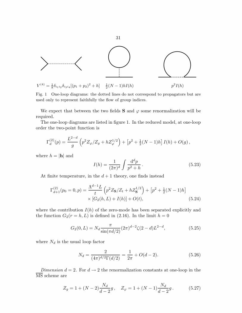
V (4) = 18δi1i2

δi3i4[(p1 + p2)

2 + h] 12(N − 1)hI(h) p2I(h)

Fig. 1 One-loop diagrams: the dotted lines do not correspond to propagators but are

used only to represent faithfully the flow of group indices.

We expect that between the two fields S and ϕ some renormalization will berequired.

The one-loop diagrams are listed in figure 1. In the reduced model, at one-looporder the two-point function is

Γ(2)d (p) =

L2−d

g

(

p2Zϕ/Zg + hZ1/2ϕ

)

+[

p2 + 12(N − 1)h

]

I(h) +O(g) ,

where h = |h| and

I(h) =1

(2π)d

∫

ddp

p2 + h. (5.23)

At finite temperature, in the d+ 1 theory, one finds instead

Γ(2)d+1(p0 = 0, p) =

Λd−1L

t

(

p2ZS/Zt + hZ1/2S

)

+[

p2 + 12 (N − 1)h

]

× [G2(h, L) + I(h)] +O(t), (5.24)

where the contribution I(h) of the zero-mode has been separated explicitly andthe function G2(r = h, L) is defined in (2.16). In the limit h = 0

G2(0, L) = Ndπ

sin(πd/2)(2π)d−2ζ(2 − d)L2−d, (5.25)

where Nd is the usual loop factor

Nd =2

(4π)d/2Γ(d/2)=

1

2π+O(d− 2). (5.26)

Dimension d = 2. For d→ 2 the renormalization constants at one-loop in theMS scheme are

Zg = 1 + (N − 2)Ndd− 2

g , Zϕ = 1 + (N − 1)Ndd− 2

g . (5.27)

32

In particular

Z/Zg = 1 +Ndd− 2

gr .

Therefore the renormalized d-dimensional two-point function reads

Γ(2)d (p) =

1

g(p2 + h) +

[

p2 + 12(N − 1)h

]

Ir(h) ,

with

Ir(h) = limd→2

I(h) +Ndd− 2

L2−d = − 1

4πln(hL2) . (5.28)

In the finite temperature theory no renormalization is required because the the-ory is non-renormalizable, and dimensional regularization cancels all power di-vergences. Thus

Γ(2)d+1(p) =

d→2

ΛL

t

(

p2 + h)

+[

p2 + 12 (N − 1)h

] (

G2(h, L) + I(h))

+O(t), (5.29)

with

G2(0, L) =Ndd− 2

− 1

2πlnL+O(d− 2) .

We note that at this order no field renormalization is required to compare thetwo functions and then

1

g=

ΛL

t+O(t).

Dimension d = 1. In d = 1 dimension the reduced theory has no divergencesand the one-loop expression reads

Γ(2)d (p) =

L

g(p2 + h) +

[

p2 + 12 (N − 1)h

]

I(h) +O(g).

We compare this expression with the finite temperature two-point function, cal-culated in the MS scheme (with renormalization scale Λ). For this purpose wehave to subtract to expression (5.25) the MS counterterm. For d→ 1 we find

[G2]r(0, L) =L

2π

(

ln(ΛL) + γ − ln(4π))

, (5.30)

and therefore

Γ(2)d+1(p) =

L

t

(

p2 + h)

+[

p2 + 12 (N − 1)h

]

[

I(h) +L

2π

(

ln(ΛL) + γ − ln(4π))

]

+O(t). (5.31)

33

This time we have also to take into account the field renormalization. We set

ϕ(x) = S(x)√

ZϕS ZSϕ = 1 + (N − 1)(

ln(ΛL) + γ − ln(4π)) t

2π,

and1

t=

1

gZtg, Zgt = 1 −

(

ln(ΛL) + γ − ln(4π)) t

2π,

or inverting the relation

1

g=

1

t− (N − 2)

2π

(

ln(ΛL) + γ − ln(4π))

+O(t),

a result which can also be obtained by the method of section 36.5 of [7]. Theresults for Zgt and g are consistent with the equations (5.15)

6 The Gross–Neveu in the large N expansion

To gain some intuition about the role of fermions at finite temperature we now ex-amine a simple model of self-interacting fermions, the Gross–Neveu (GN) model.The GN model is described in terms of a U(N) symmetric action for a set of Nmassless Dirac fermions ψi, ψi:

S(

ψ, ψ)

= −∫

dd+1x[

ψ · 6∂ψ + 12G

(

ψ · ψ)2

]

. (6.1)

The GN model has in all dimensions a discrete symmetry

x = x1, x2, . . . , xd 7→ x = −x1, x2, . . . , xd,

ψ(x) 7→ γ1ψ(x),ψ(x) 7→ −ψ(x)γ1

,

which prevents the addition of a mass term. In even dimensions it implies adiscrete chiral symmetry, and in odd dimensions it corresponds to space reflec-tion. Below, to simplify, we will speak about chiral symmetry, irrespective ofdimensions.

The GN model is renormalizable in d = 1 dimension, where it is asymptoticallyfree and the chiral symmetry is always broken at zero temperature.

We recall that within the 1/N expansion it can be proven that the GN model isequivalent to the GNY (Y for Yukawa) model, a model with the same symmetry,but with an elementary scalar particle coupled to fermions through a Yukawa-like interaction, which is renormalizable in four dimensions [25]. This equivalenceprovides a simple interpretation to some of the results that follow.

Since fermions at finite temperature have no zero modes, limited insight aboutthe physics of the model can be gained from perturbation theory; all fermionsare simply integrated out. Therefore we study here the GN model within theframework of the 1/N expansion.

34

6.1 The GN model at zero temperature, in the large N limit

We first recall the properties of the GN model at zero temperature [26,25] inthe large N limit. To generate the large N expansion one introduces an auxiliaryfield σ, replaces the action (6.1) by an equivalent action:

S((

ψ, ψ, σ)

=

∫

dd+1x

[

−ψ · (6∂ + σ)ψ +1

2Gσ2

]

,

and integrates over N − 1 fermions. One finds (ψ ≡ ψ1)

SN(

ψ, ψ, σ)

=

∫

dd+1x

[

−ψ(6∂ + σ)ψ +1

2Gσ2

]

− (N − 1) tr ln (6∂ + σ) . (6.2)

For G = O(1/N) the corresponding partition function can be calculated bythe steepest descent method. The saddle point (or gap) equation obtained bydifferentiating with respect to σ has the trivial solution σ = 0 and (at leadingorder for N → ∞ we can replace N − 1 by N)

1

G=

N ′

(2π)d+1

∫ Λ dd+1k

k2 + σ2, (6.3)

where N ′ = N tr1 is the total number of fermions.Note that at leading order forN large the scalar field expectation value σ = 〈σ〉

is also the fermion mass mψ = 〈σ〉.For d = 1 the chiral symmetry is spontaneously broken for all G > 0, and one

findsσ = mψ ∝ Λ e−π/NG .

For d > 1 a phase transition occurs at a value Gc such that

1

Gc=

N ′

(2π)d+1

∫ Λ dd+1k

k2.

For G < Gc the saddle point is σ = 0 and the chiral symmetry is preserved. ForG > Gc the chiral symmetry is broken, and for d < 3

σ ∝ (G−Gc)1/(d−1),

which implies that the physical region corresponds to |G−Gc| small.For d = 3 logarithmic corrections appear and one finds instead

σ2 ln(Λ/σ) ∼ 8π2

N ′

(

1

Gc− 1

G

)

,

a reflection of the IR triviality of the effective renormalizable GNY model.

35

In higher dimensions the model is equivalent to a weakly interacting GNYmodel, with an IR stable gaussian fixed point and

σ ∝ (G−Gc)1/2.

In the broken phase the σ-propagator is given by

∆−1σ (p) =

N ′

2(2π)d+1

(

p2 + 4σ2)

∫ Λ dd+1k

(k2 + σ2) [(p+ k)2 + σ2], (6.4)

where the saddle point equation has been used. The mass of the scalar fieldmσ = 2 〈σ〉, is such at leading order the σ particle is a fermion bound state atthreshold (mσ = 2mψ).

In the chiral symmetric phase G < Gc instead one finds

∆−1σ (p) =

1

G− 1

Gc+

N ′

2(2π)d+1p2

∫ Λ dd+1k

k2(p+ k)2, (6.5)

a reflection of the property that the σ particle now is a resonance which candecay into a fermion pair.

6.2 The GN model at finite temperature

Due to the anti-periodic boundary conditions fermions have no zero modes, andat high temperature can be integrated out, yielding an effective action for theperiodic scalar field σ. In the situations in which the σ mass is small comparedwith the temperature, one can perform a mode expansion of the σ field, integrateover the non-zero modes and obtain a local d-dimensional action for the zero-mode. It is important to realize that, since the reduced action is local andsymmetric in σ 7→ −σ, it describes the physics of the Ising transition with shortrange interactions (unlike what happens at zero temperature). The questionwhich then arises is the possibility of a breaking of this remaining symmetry ofIsing type. If a transition exists and is continuous, the σ-mass vanishes at thetransition and a potential IR problem appears.

Additional effects due to the addition of a chemical potential will not be con-sidered in these notes [27].

After integration over all fermions we obtain a non-local action SN for thefield σ,

SN (σ) =1

2G

∫ L

0

dτ

∫

ddxσ2 −N tr ln (6∂ + σ) , (6.6)

where L is the inverse temperature T = 1/L, and the σ field satisfies periodicboundary conditions in the time direction. As we have seen a non-trivial pertur-bation theory is obtained by expanding for large N .

36

The gap equation. The gap equation at finite temperature again splits intotwo equations σ = 0 and

L

G= N ′G2(σ, L), (6.7)

G2(σ, L) =1

(2π)d

∑

n

∫ Λ ddk

k2 + ω2n + σ2

, ωn = (2n+ 1)π/L .

Using Schwinger’s representation, and the corresponding regularization, the func-tion G2 can be expressed in terms of another function ϑ1(s), of elliptic type(equation (A2.15)),

G2(σ, L) =L2−d

4π

∫

s0

ds

sd/2e−sL

2σ2/(4π) ϑ1(s), (6.8)

with s0 = 4π/(ΛL)2. From equation (A2.16) we learn that ϑ1(s) = 1/√s for

s→ 0, up to exponentially small corrections. The function G2(σ, L) has a regularsmall σ expansion. The two first terms are

G2(σ, L) = G2(0, L) + σ2G4 +O(σ4),

with for d < 5 (equations (A1.6,A1.5))

G2(0, L) =4L2−d

(4π)(d+1)/2(1 − 2d−2)Γ

(

(d− 1)/2)

ζ(d− 1) +1

d− 1

2LΛd−1

(4π)(d+1)/2(6.9)

G4 = L4−dΓ(2 − d/2)

8π4−d/2

(

24−d − 1)

ζ(4 − d) +1

d− 3

2LΛd−3

(4π)(d+1)/2. (6.10)

Finally the propagator ∆σ(p) ≡ ∆σ(ω = 0, p) of the σ zero-mode, in the brokenphase, is given by (after use of the gap equation (6.7))

∆−1σ (p) =

N ′

2(2π)dL

(

p2 + 4σ2)

∑

n

∫ Λ ddk

(k2 + ω2n + σ2) [(p+ k)2 + ω2

n + σ2].

(6.11)We again find that the σ-mass is 2σ. In the symmetric phase instead the prop-agator of the zero mode is given by

1

N ′∆σ(p)=

1

N ′G− G2(0, L)

L+

p2

2(2π)dL

∑

n

∫ Λ ddk

(k2 + ω2n)[(p+ k)2 + ω2

n].

(6.12)

37

6.3 Phase structure for d > 1

For d > 1 we introduce the critical value Gc where σ vanishes at zero temper-ature (L = ∞),

[G2]r(σ, L) = G2 −L

N ′Gc=L2−d

4π

∫

s0

ds

sd/2

[

e−sL2σ2/(4π) ϑ1(s) − s−1/2

]

, (6.13)

The function [G2]r(σ, L) is a decreasing function of σ, thus

[G2]r(σ, L) ≤ [G2]r(0, L) = L2−dI2(d), (6.14)

with

I2(d) =4

(4π)(d+1)/2

(

1 − 2d−2)

Γ(

(d− 1)/2)

ζ(d− 1). (6.15)

The integral is always negative and therefore the gap equation (6.7) has a solutiononly for G > Gc, i.e. when at zero temperature chiral symmetry is broken. Ford < 3 the integral (6.13) converges at s = 0 and the gap equation (6.7) takes ascaling form. For d = 2 it can be expressed in terms of the fermion mass at zerotemperature mψ

Lmψ = −∫

0

ds

s

(

e−sL2σ2/(4π) ϑ1(s) − s−1/2

)

.

The phase transition. A phase transition between the two Ising phases takesplace at a temperature Tc = L−1

c where σ solution to the equation (6.7) vanishes:

Ld−1c

(

1

G− 1

Gc

)

= N ′I2(d).

Since the r.s.h. of the gap equation (6.7) is a decreasing function of σ, the σ → −σIsing symmetry is broken for T < Tc and restored for T > Tc.

It is interesting to express the critical temperature in terms of the fermionmass mψ. For d > 3 one finds

Tc = (Lc)−1 ∝ mψ(Λ/mψ)(d−3)/(d−1) ≫ mψ .

Therefore the critical temperature is a high temperature in the scale of theparticle masses.

For d = 3 the critical temperature is given by

L2c

(

1

Gc− 1

G

)

=N ′

48.

38

Therefore

Tc ∼√

6

πmψ

√

ln(Λ/mψ) ∝√

G−Gc,

which again corresponds to a high temperature regime.Finally for d = 2 the critical temperature is proportional to the fermion mass:

Tc =1

2 ln 2mψ .

Local expansion. When the σ mass or expectation value are small comparedto 1/L we can perform a local expansion of the action (6.6), and study it toall orders in the 1/N expansion. Consistency requires that one also performs amode expansion of the field σ and retains only the zero mode. In the reducedtheory 1/L plays the role of a large momentum cut-off.

The first terms of the effective d dimensional action are

Sd(σ) =

∫

ddx

[

12Zσ(∂µσ)2 + 1

2rσ2 +

1

4!uσ4

]

, (6.16)

where terms of order σ6 and ∂2σ4 and higher have been neglected, and the threeparameters are given by

Zσ = 12N

′G4 , r =L

G−N ′G2(0, L) , u = 6N ′G4 ,

where G4 = L4−dI4(d). For d > 1 after the shift of the coupling constant onefinds

r =L

G− L

Gc−N ′L2−dI2(d) = N ′I2(d)L

(

L1−dc − L1−d

)

. (6.17)

Though, after rescaling of the field we observe that the effective σ4 couplingis logarithmically small, close enough to the critical temperature the effectivetheory cannot be solved by perturbative methods.

For d = 2 the integrals are UV finite after the shift of G. The effective theorydescribes the physics of the two-dimensional Ising model.

Dimensional reduction and σ mass. For d > 3, in the symmetric phase L < Lc,the σ mass behaves like

m2σ ∝ L−2(ΛL)3−d

[

1 − (L/Lc)d−1

]

,

and thus is small with respect to L, justifying dimensional reduction. Moreover,

after rescaling of the field σZ1/2σ 7→ σ one sees that the effective σ4 coupling is

of orderu/Z2

σ ∝ Ld−4(ΛL)3−d.

39

For d ≥ 4 the coupling is small, the physics perturbative, and no additionalanalysis is required.

For the mathematical case 3 < d < 4, the situation is more subtle. Fordimensional reasons the true expansion parameter is

md−4σ u/Z2

σ ∝ (mσL)d−4(ΛL)3−d.

At high temperature, i.e. for 1 − L/Lc positive and finite, Lmσ ∝ (ΛL)(3−d)/2

and one findsmd−4σ u/Z2

σ ∝ (ΛL)(3−d)(d−2)/2,

which is small. On the other hand for |T−Tc| ∝ L−Lc small enough perturbationtheory is no longer useful.

For d = 3 dimensional reduction is justified near the critical temperature,but the reduced model is non-perturbative. Since the coefficient G4 has still alogarithmic UV contribution, in the symmetric phase at high temperature onefinds

Lmσ ∝ 1/√

ln(ΛL),

which also justifies a local expansion. The effective coupling

u

mσZ2σ

∝ 1√

ln(ΛL),

and thus the reduced model can be solved using perturbation theory. This is asituation we have already met in the example of the φ4 field theory, and whichreflects the IR triviality of the GNY model.

In dimension d = 2, near the critical temperature the σ mass is small and alocal and mode expansions can be performed. The reduced theory cannot besolved by perturbation theory.

In general the model obeys simple scaling relations (a reflection of the existenceof a non-trivial IR fixed point in the GNY model). At high temperature σ = 0,and the σ mass if of order 1/L. No local expansion is justified and necessary.

6.4 Dimension d = 1

The situation d = 1 is doubly special, since at zero temperature chiral symmetryis always broken and at finite temperature the Ising symmetry is never broken.The GN model is renormalizable and UV free

β(G) = −N′ − 2

2πG2 +O(G3).

The RG invariant mass scale Λ(G), to which all masses at zero temperature ofthe rich GN spectrum are proportional, has the form

Λ(G) ∝ Λ exp

[

−∫ G dG′

β(G′)

]

.

40

Physical masses are small with respect to Λ when G is small

ln(Λ/mψ) =2π

(N ′ − 2)G+O(lnG).

At finite temperature all masses, in the sense of inverse of the correlation lengthin the space direction, have a scaling property. For example the σ mass has theform

Lmσ = f(Lmψ).

One can also express the scaling properties by introducing a temperature depen-dent coupling constant GL defined by

∫ GL

G

dG′

β(G′)= − ln(LΛ).

At high temperature GL decreases

GL ∼ 2π

(N ′ − 2) ln(Lmψ).

We therefore expect a trivial high temperature physics with weakly interactingfermions.

At finite temperature the large N gap equation becomes

2π

N ′G= ln(ΛL) +

1

2

∫

0

ds

s1/2

[

e−L2σ2s/(4π) ϑ1(s) − s−1/2θ(1 − s)

]

,

which, in terms of the zero-temperature mass scale

mψ = Λ e−2π/N ′G,

can be rewritten:

ln(mψL) = F (σL),

F (z) = −1

2

∫

0

ds

s1/2

[

e−z2s/(4π) ϑ1(s) − s−1/2θ(1 − s)

]

.

The function F (z) is an increasing function, with a finite limit for z → 0 andwhich behaves like ln z for z → ∞, in such a way that at low temperatureone recovers mσ = 2mψ. Again we find a phase transition at a temperatureL−1c ∝ mψ. This mean-field-like prediction of a phase transition contradicts the

well-known property of the absence of phase transitions in an Ising-type modelin d = 1 dimension. In the high temperature phase σ = 0 and one finds

1

N ′∆σ(p)=

1

2π

[

− ln(Lmψ) − γ + 12

lnπ]

+∑

n≥0

p2

Lωn(p2 + 4ω2n),

41

from which one derives a scaling relation

Lmσ = f(Lmψ).

If we assume that dimensional reduction is justified we can return to the ac-tion (6.16). At leading order we find a simple model in quantum mechanics:the quartic anharmonic oscillator. Straightforward considerations show that thecorrelation length, inverse of the σ mass parameter, becomes small only whenthe coefficient of σ2 is large and negative. This happens only at low temperature,where the two lowest eigenvalues of the hamiltonian corresponding to space direc-tion are almost degenerate, a precursor of the zero temperature phase transition.One then finds

Lmσ ∝ (lnmψL)5/4 e−const.(lnmψL)3/2 .

7 Abelian gauge theories

We first discuss the abelian case which is much simpler, because the mode de-composition is consistent with the gauge structure. Some additional problemsarising in non-abelian gauge theories will be considered in next section. Becausethe gauge field has a number of components which depends on the number ofspace dimensions, the mode expansion have some new properties and affectsgauge transformations. The simplest non-trivial example of a gauge theory isQED, a theory which is IR free in four dimensions, and therefore from the RGpoint of view has properties similar to the scalar φ4 field theory. Another exam-ple is provided by the abelian Higgs model but since it has a first order phasetransition, it has a more limited validity.

7.1 Mode expansion and gauge transformations

We decompose a general gauge field Aµ(t, x) into the sum of a zero mode Bµ(x)and the sum of all non-zero modes Qµ(t, x)

Aµ(t, x) = Bµ(x) +Qµ(t, x).

At finite temperature T = L−1, Qµ(t, x) thus satisfies

∫ L

0

dtQµ(t, x) = 0 . (7.1)

With this decomposition gauge transformations

δAµ(t, x) = ∂µϕ(t, x),

become

δBµ(x) = ∂µϕ0(t, x), δQµ(t, x) = ∂µϕ1(t, x) , ϕ = ϕ0 + ϕ1 . (7.2)

42

Since δBµ does not depend on t we conclude that ϕ0(t, x) must have the specialform

ϕ0(t, x) = F (x) + Ωt , (7.3)

where Ω is a constant. The space components Bi transform as the componentsof a d-dimensional gauge field; the time component B0 is a d-dimensional scalarfield which is translated by a constant

δB0(x) = Ω . (7.4)

Symmetry which respect to the translation (7.4) implies that the scalar field B0

is massless.

The condition (7.1) then implies

∂i

∫ L

0

dt ϕ1(t, x) = 0 ,

∫ L

0

dt ∂tϕ1(t, x) = 0 ⇒ ϕ1(0, x) = ϕ1(L, x).

The transformations of the gauge field Qµ are thus specified by periodic functionsϕ1(t, x) with a constant zero-mode, which can be set to zero.

Finally we verify that the function ϕ = ϕ1 + ϕ0 is such that ∂µϕ is periodicas it should, since Aµ is periodic.

Matter fields. We now couple the gauge field to matter, for instance chargedfermions ψ(t, x), ψ(t, x). At finite temperature fermion fields satisfy anti-periodicboundary conditions. To the gauge transformation (7.2) corresponds for thefermions

ψ(t, x) = eiϕ(t,x) ψ′(t, x), ψ(t, x) = e−iϕ(t,x) ψ′(t, x).

Anti-periodicity implies that

ϕ(L, x) = ϕ(0, x) (mod 2π) .

Since ϕ1 is periodic, the condition implies for the constant Ω in (7.3)

Ω = 2nπ/L . (7.5)

This restriction on the transformation (7.4) of the scalar component B0 hasimportant consequences. As a result of quantum corrections generated by theinteractions with charged matter, the scalar field B0 does not remain massless.Instead the thermodynamic potential is a periodic function of B0 with period2π/L.

43

7.2 Gauge field coupled to fermions: quantization

We now consider a gauge field coupled to an N -component massless chargedfermion

S(

ψ, ψ, Aµ)

=

∫

dd+1x[

14e2F 2µν(x) − ψ(x) · (6∂ + i 6A)ψ(x)

]

. (7.6)

The theory has RG properties which bear some similarities with the φ4 theory;it is renormalizable for d = 3 and IR free (trivial). It can be solved in the largeN limit. Finally in dimension d = 1 it reduces to the massless Schwinger modelwhich can be solved exactly even at finite temperature [28], because bosonizationmethods still work.

The temporal gauge. To calculate the partition function we first quantize in thetemporal gauge A0(x, t) = 0 because the corresponding hamiltonian formalismis simple. The action becomes

S(

ψ, ψ, Aµ)

=

∫

ddxdt[

14e2

(

2A2i + F 2

ij(t, x))

− ψ(t, x) · (6∂ + i 6A)ψ(t, x)]

.

(7.7)In calculating tr e−LH we have to remember that Gauss’s law has still to beimposed. This means that the trace has to be taken in the subspace of wavefunctionals invariant under space-dependent gauge transformations. To projectonto this subspace we impose periodic conditions in the time direction up to agauge transformation:

Ai(L, x) = Ai(0, x)− L∂iϕ(x),

ψ(L, x) = eiLϕ(x) ψ(0, x),

and integrate over the gauge transformation ϕ(x). We then set

Ai(t, x) = A′i(t, x)− t∂iϕ(x),

ψ(t, x) = eitϕ(x) ψ′(t, x).

where the fields A′i, ψ

′, ψ′ now are periodic and anti-periodic resp.. This inducestwo modifications in the action

∫

dxdt (∂tAi)2 7→

∫

dxdt (∂tAi)2 + L

∫

dx (∂iϕ(x))2

∫

dxdt ψ(t, x)γ0∂tψ(t, x) 7→∫

dxdt ψ(t, x)γ0(∂t + iϕ(x))ψ(t, x).

Therefore ϕ(x) is simply the residual zero mode of the A0 component

ϕ(x) ≡ B0(x).

44

Its presence is a direct consequence of enforcing Gauss’s law.The field theory has a d-dimensional gauge invariance with the zero modeBi(x)

of Ai(t, x) as gauge field. In addition it contains d families of neutral vector fieldswith masses 2πn/L, n 6= 0, quantized in a unitary, and thus non-renormalizablegauge.

Note that from the technical point of view the usual difficulties which appearin perturbation calculations with the temporal gauge (the gauge field propagatoris singular) reduce to the need for quantizing the remaining zero-mode, and tothe non explicit renormalizability. The latter problem can be solved with thehelp of dimensional regularization for example (for gauge invariant observables).An alternative possibility of course is to introduce a renormalizable gauge. Thechange of gauges can be performed by the standard zero-temperature method[7].

Covariant gauge. To change to the covariant gauge we introduce a time com-ponent A0 for the gauge field (periodic in time) and multiply the functionalmeasure by the corresponding δ-function

1 =

∫

[dQ0(t, x)]∏

t,x

δ(Q0).

The action can then be written in a gauge invariant form. We then introduce asecond identity in the functional integral

1 = det(−∂2)

∫

[dϕ1]δ(

∂µQµ + ∂2ϕ1 − h(t, x))

, (7.8)

where ϕ1 and h(t, x) are two periodic functions without zero-mode. We performthe gauge transformation

Qµ + ∂µϕ1 7→ Qµ .

The ϕ1 dependence remains only in δ(Q0 − ∂tϕ1), and the integration over ϕ1

yields a constant. Integration over h(t, x) with a gaussian weight yields thestandard covariant gauge

Sgauge =L

2ξ

∫

dx(

∂iBi(x))2

+1

2ξ

∫

dtdx(∂µQµ)2 ≡ 1

2ξ

∫

dtdx(∂µAµ)2.

since∂µAµ = ∂tQ0(t, x) + ∂iBi(x) + ∂iQi(t, x).

We conculde that the gauge fixing term is just obtained by substituting the modedecomposition into the gauge fixing term of the zero-temperature action. Fromthe point of view of the B gauge field this corresponds to a quantization in thecovariant gauge in d dimensions.

Note that the transformation from the temporal gauge to the covariant gaugegenerates a determinant (equation (7.8)) which is field-independent, but con-tributes to the free energy.

45

7.3 Dimensional reduction

At finite temperature, to generate the effective action for the gauge field zero-modes, we have to integrate over all fermion modes (anti-periodic boundaryconditions) and over the non-zero modes Qµ(t, x) of the gauge field. At leadingorder one finds a free theory containing a gauge field Bi and a massless scalarB0. At one-loop order only fermion modes contribute. Replacing the gauge fieldAµ by its zero mode Bµ and performing the fermion integration explicitly wefind the effective action

SL = L

∫

ddx

[

1

2e2(∂iB0)

2 +1

4e2F 2ij(B)

]

−N tr ln (6∂ + i6B) , (7.9)

where latin indices means space indices.An important issue is the behaviour of induced mass of the time component

B0 = ϕ of the gauge field. We thus first calculate the effective potential forconstant ϕ.

The effective potential. The effective potential for constant field ϕ is then givenby

V (ϕ) = −12N

′∑

n

1

(2π)d

∫

ddk ln[

k2 +(

ϕ+ (2n+ 1)π/L)2

]

,

where N ′ = N tr1 is the total number of fermion degrees of freedom.Its evaluation involves the new function

∑

n

e−t[(2n+1)π/L+ϕ]2 ≡ ϑ2(4πt/L2; ν, 0) =

L

2√πt

∑

n

(−1)n cos(nLϕ) e−n2L2/4t,

where ν = 12 +Lϕ/2π, and the general Poisson’s formula (A2.13) has been used.

Then

V (ϕ) = 12N ′ 1

(4π)d/2

∫

dt

t1+d/2[

ϑ2(4πt/L2; ν, 0)− ϑ2(4πt/L

2; 1/2, 0)]

, (7.10)

where V (ϕ) has been shifted so as to vanish for ϕ = 0. After the usual changeof variables t = L2s/4π we find

V (ϕ) = 12N

′L−d

∫ ∞

s0

ds

s1+d/2[ϑ2(s; ν, 0)− ϑ2(s; 1/2, 0)] , (7.11)

We note

ϑ2(s; ν, 0)− ϑ2(s; 1/2, 0) = s−1/2∑

n

(−1)n+1 [1 − cos(nLϕ)] e−n2π/s,

46

which shows that the n = 0 term cancels and thus the potential is UV finite.This is not too surprising since in the zero temperature, large L, limit no gaugefield mass or quartic potential are generated.

The potential has an extremum at ϕ = 0. The coefficient of ϕ2 is:

V (ϕ) = 12L2−dϕ2K2(d) +O(ϕ4)

K2(d) = N ′ 8

(4π)d/2+1/2Γ(

(d+ 1)/2) (

2d−2 − 1)

ζ(d− 1).

The constant K2(d) is positive showing that ϕ = 0 is a minimum. More generallythe potential is

V (ϕ) = K(d)L−dV(Lϕ) , K(d) = N ′ 1

πd/2+1/2Γ(

(d+ 1)/2)

,

where the function V(z) is given by the sum

V(z) =∑

n=1

(−1)n+1

(

1 − cos(nz))

nd+1=

1 − cos z

2Γ(d+ 1)

∫ ∞

0

dττd tanh(τ/2)

cosh τ + cos z.

Its derivative has the sign of sin z, it is negative for −π < z < 0 and positive for0 < z < π. Therefore z = 0 is the unique minimum in the interval −π < z < π.

A special case is d = 1 for which one finds

V ′(z) = 12z for |z| < π and thus V(z) = 1

4z2.

To obtain the mass of ϕ field at this order it is necessary to also calculate thecoefficient of (∂iϕ)2 generated by the determinant. Expanding to order p2 theFourier transform of the coefficient of ϕϕ/2 in SL we find

S(2)L (p) =

Lp2

e2+N ′

∑

n

∫

ddk

(2π)d

[

ω2n − k2

(k2 + ω2n)

2+p2

6

3k2 − ω2n

(k2 + ω2n)

3

]

+O(p4).

The coefficient of (∂iϕ)2 is renormalized and for d < 3 becomes

L

2e2(∂iϕ)2

[

1 +N ′L3−dK3(d)e2]

,

with

K3(d) =1

(4π)d/2d− 1

3(1 − 2d−4)Γ(2 − d/2)ζ(4− d),

(which vanishes for d = 1 as expected from the exact solution of the Schwingermodel). For d ≥ 3 one has to add to K3(d) a cut-off dependent contribution

47

generated for instance by a Pauli–Villars regulator field, a fermion of large massΛ,

1

3(4π)(d+1)/2Γ(

(3 − d)/2)

(ΛL)d−3.

These contributions generate in dimensions d ≥ 3 a renormalization e 7→ er ofthe coupling constant.

Discussion. We thus obtain a mass term which is proportional to erL(1−d)/2.

If e is generic, i.e. of order 1 at the microscopic scale 1/Λ, then e ∝ Λ(3−d)/2 andthe scalar mass is proportional to (ΛL)(3−d)/2/L. It is thus large with respectto the vector masses for d < 3 and small for d > 3. We conclude that for d < 3the scalar field can be completely integrated out, but for d > 3 it survives. Notethat for d > 3 additional corrections are even smaller because UV divergencescannot compensate the small coupling constant. For d = 3 QED is IR free,

βe2 =N

6π2e4 +O(e6),

er has to be replaced by the effective coupling constant e(1/ΛL) with is logarith-mically small

e2(1/ΛL) ∼ 6π2

N ln(ΛL),

and the scalar mass thus is still small

m2ϕ ∝ 1

L2 ln(ΛL).

The separation between zero and non-zero modes remains justified. The situationis completely analogous to high temperature φ4 field theory, and perturbationfor the same reason remains applicable.

Finally if one is interested in IR physics only, one can in a second step integrateover the massive scalar field ϕ.

For more details and more systematic QED calculations see [29,30,31].

7.4 The abelian Higgs model

The abelian gauge fields interacting with charged scalar fields has also beeninvestigated [32,33,30] as a toy model to study properties of the electro-weakphase transition at finite temperature. The gauge action reads

S(Aµ, φ) =

∫

dtddx

[

1

4e2F 2µν + |Dµφ|2 + U(|φ|2)

]

, (7.12)

where the quartic potential U(|φ|2)

U(z) = rz + 16gz

2, (7.13)

48

is such that the U(1) symmetry is broken at zero temperature.The model can directly be quantized in the unitary (non-renormalizable) gauge

and calculations of gauge-independent observables can be performed with di-mensional regularization. Below we use instead the temporal gauge because theunitary gauge becomes singular near the phase transition.

One limitation of the model is that RG shows that in 3 + 1 dimensions thehypothesis of second order phase transition is inconsistent, and therefore thetransition is most likely first order. Indeed, in a more general model with Ncharged scalars for d = 3 the RG β-functions are

βg =1

24π2

[

(N + 4)g2 − 18ge2 + 54e4]

βe2 =1

24π2Ne4.

The origin e2 = g = 0 is a stable IR fixed point only for N ≥ 183. For N small,the continuum model remains meaningful if initially the coupling constants aresmall enough, in such a way that by the time the running coupling contantsreach the physical scale, they have not yet reached the region of instability. Thetransition then is weak first order.

Presumably the same result applies for small values of N to the three-dimen-sional classical statistical field theory, which is also the Landau–Ginzburg modelof superconductivity.

Neglecting all non-zero modes we obtain one massive vector field degeneratedin mass with a scalar field, and the Higgs field. We expect the degeneracy betweenvector and scalar masses to be lifted by the integration over non-zero modes. Toconstruct the reduced action we quantize in the temporal gauge A0 = B0 andwe set

Ai = Bi +Qi , φ = ϕ+ χ .

The reduced action at leading order is simply

SL(Bµ, ϕ) = L

∫

ddx

[

1

2e2(∂iB0)

2 +1

4e2F 2ij(B) + |Diϕ|2 + |ϕ|2B2

0 + U(|ϕ|2)]

,

(7.14)where the covariant derivative now refers to the gauge field Bi

Di = ∂i + iBi .

At one-loop order we need the terms quadratic in Qµ, χ. In the gaussian inte-gration over Qµ, χ at high temperature the leading effects come from the shiftin the masses. We can therefore take B0 and ϕ constant. The quadratic termsin the action relevant for the ϕ mass shift are

S2 =

∫

dtddx

[

1

2e2(∂tQi)

2 +1

4e2F 2ij(Q) + |∂tχ|2 + |∂iχ+ iQiϕ|2 + 2

3g|ϕ|2|χ|2

]

,

49

where we have omitted the term proportional to r|χ|2, a high temperature ap-proximation. The integration over χ yields a term

e2|ϕ|2∑

ω

∫

ddk Qi(ω, k)

(

δij −kikj

k2 + ω2

)

Qj(−ω,−k) ,

and thus finally a contribution δr to the coefficient of |ϕ|2

δr = G2(0, L)(de2 + 2g/3)/L ,

where G2 is defined by equation (2.16). For d = 3 we have found G2 = 1/12L(section 3.2) and therefore

δr =1

36L2(9e2 + 2g).

For the contribution to the B0 mass the relevant quadratic action is

S2 =

∫

dtddx|Dµχ|2.

In the limit of constant Bµ, the space components Bi can be eliminated bya gauge transformation. The remaining B0 component cannot be eliminatedbecause χ satisfies periodic boundary conditions in the time direction. Instead,as we have already discussed, the mode integration generates a periodic potentialfor B0

∫

ddx∑

ω

∫

ddk ln[

(

ω +B0(x))2

+ k2]

.

Expanding to order B20 we obtain the mass term

(d− 1)G2

∫

ddxB20(x),

where the identity, valid in dimensional regularization,

1

(2π)d

∑

ω

∫

ddk ω2

(k2 + ω2)2= (1 − d/2)G2 ,

has been used. Thus for d = 3

m2B0

=e2

3L2.

As we have discussed several times, in three dimensions additional UV contribu-tions transform the parameters e2, g, r into the one-loop expansion of the running

50

parameters at scale 1/ΛL. Finally, for completeness, let us point out that thecoefficient of |ϕ|2B2

0 gets renormalized. At one-loop one finds

1 7→ 1 +e2 + g

12π2.

Discussion. We assume that at zero temperature the U(1) symmetry is bro-ken which implies that the coefficient r in the potential U (equation (7.13)) issufficiently negative. When the temperature increases, the coefficient of |ϕ2|increases until a critical temperature is reached where the U(1) symmetry isrestored. Near the transition the scalar field B0 is massive and therefore the ef-fective theory relevant for the phase transition is simply the classical U(1) gaugemodel

SL(Bi, ϕ) = L

∫

ddx

[

1

4e2F 2ij + |Diϕ|2 + U(|ϕ|2)

]

, (7.15)

where the parameters e2 and in U can be obtained by integrating the reducedaction also over the heavy field B0.

8 Non-abelian gauge theories

Pure non-abelian gauge theories, as well as non-abelian gauge coupled to a smallnumber of fermions, are UV asymptotically free in four dimensions. From theRG point of view, we expect some similarities with the non-linear σ model (indifferent dimensions). In particular in d = 3 dimensions the effective couplingconstant g(L) decreases at high temperature, g(L) ∝ 1/ ln(mL), where m is theRG invariant mass scale of the gauge theory.

Notation. We consider fields Aµ written as matrices in the adjoint represen-tation of some compact group G. Gauge transformations take the form

A′µ(x) = g(x)Aµ(x)g

−1(x) + g(x)∂µg−1(x), (8.1)

where g is a group element.Covariant derivatives Dµ acting on fields ϕ belonging the adjoint representa-

tion areDµϕ = ∂µϕ+ [Aµ, ϕ] . (8.2)

The corresponding curvature Fµν(x) tensor is

Fµν(x) = [Dµ,Dν ] = ∂µAν − ∂νAµ + [Aµ,Aν] , (8.3)

and the pure gauge action

S(A) = − 1

4g2tr

∫

dd+1xF2µν . (8.4)

51

Temporal gauge. The situation is here more complicated because the mode de-composition is not gauge invariant. Thus we first quantize, choosing the temporalgauge. Then the space components Ai must be periodic up a gauge transforma-tion which again enforces Gauss’s law:

Ai(L, x) = g(x)Ai(0, x)g−1(x) + g(x)∂ig

−1(x),

We parametrize the group element g in terms of an element ϕ of the Lie algebra:

g(x) = eLϕ(x),

and introduceg(t, x) = etϕ(x),

After the gauge transformation

Ai(t, x) = g(t, x)A′i(t, x)g

−1(t, x) + g(t, x)∂ig−1(t, x),

the new field A′i becomes strictly periodic. The gauge component A0 which

vanishes before the transformation becomes

0 = g(t, x)A′0(t, x)g

−1(t, x) + g(t, x)∂tg−1(t, x),

and thereforeA′

0(t, x) = ϕ(x).

Again the temporal gauge reduces the time-component A0 to its zero-mode, thefield ϕ(x).

Let us express the pure gauge action (8.4) in terms of the new fields

S(A, ϕ) = − 1

2g2tr

∫

dtddx(

∂iϕ(x) − ∂tAi + [Ai, ϕ])2 − 1

4g2tr

∫

dtddxF2ij

= − 1

2g2tr

∫

dtddx (Diϕ− ∂tAi)2 − 1

4g2tr

∫

dtddxF2ij .

Dimensional reduction. We now separate the zero-modes of the space compo-nents of the gauge field

Ai(t, x) = Bi(x) + Qi(t, x),

withQi(t, x) =

∑

n6=0

e2iπnt/LQn,i(x).

ThenDi(A)ϕ = Di(B)ϕ+ [Qi, ϕ].

52

In the same way

Fij(A) = Fij(B) + DiQj −DjQi + [Qi,Qj],

where the covariant derivative now refers to the gauge field B.We see that the resulting action is gauge invariant with respect to time-

independent gauge transformations with gauge field B. The gauge field is cou-pled to a massless scalar ϕ and massive vector fields with masses 4π2n2/L2, allbelonging to the adjoint representation.

The problem of quantization then reduces to the quantization of the field B. Ifwe choose a covariant gauge then, not only is the theory quantized, but the vectorfields do not have the kind of singular propagator typical of the temporal gauge.A question remains, massive vector fields lead to non-renormalizable theories. Away to solve this problem is to go over to a covariant gauge. We introduce a timecomponent A0 for the gauge field (periodic in time) and multiply the functionalmeasure by the corresponding δ-function. The action is a function only of thesum A0(t, x) + ϕ(x). Let us thus temporarily call Aµ the field

Ai = Ai , A0 = A0(t, x) + ϕ(x).

The δ-function then becomes δ(A0 − ϕ). We then perform the standard manip-ulations to pass to the covariant gauge with gauge function ∂µAµ. Eventually

we shall get the gauge average of the constraint δ(A0−ϕ). This gives a determi-nant which only depends on ϕ, while ϕ appears nowhere else. The integral overϕ factorizes and gives a constant factor. Of course in the process we have intro-duced ghost fields which satisfy periodic boundary conditions, unlike ordinaryfermions.

One-loop calculation of the effective ϕ potential. We expect that quantumcorrections generated by the integration over non-zero modes give a mass to thescalar field ϕ, as in the abelian example.

For ϕ constant, and omitting the massless gauge field we find a simplifiedaction. It is convenient here to introduce the generators of the Lie algebra of thecompact group G, in the form of hermitian matrices τα

tr τατβ = δαβ , [τα, τβ] = ifαβγτγ ,

where the structure constants fαβγ are chosen antisymmetric. We then set

Qi = iQαi τα , ϕ = iϕατα.

Then the relevant Q action is

S2(Q) =1

2g2

∫

dtddx

[

12

(

∂iQαj − ∂jQ

αi

)2+

(

∂tQαi + fαβγQ

βi ϕ

γ)2

]

.

53

The integration yields a determinant which generates an additive contributionto the effective action

V (ϕ) = 12

∑

n6=0

tr ln[(

k2δij − kikj + ω2nδij

)

δαβ + δij (2iωnfαβγϕγ + fαγδfβǫδϕ

γϕǫ)]

− (ϕ = 0), (8.5)

with ωn = 2πn/L. The result can be written as the sum of two contributions,along k and transverse. The first contribution is

V1(ϕ) = 12

∑

x

∑

n6=0

tr ln[

ω2nδαβ + (2iωnfαβγϕ

γ + fαγδfβǫδϕγϕǫ)

]

− (ϕ = 0)

=∑

x

∑

n6=0

tr ln (δαβ + ifαβγϕγ/ωn) .

= lndet

[

∏

x

2Φ−1L−1 sinh(LΦ/2)

]

, (8.6)

where we have introduced the matrix Φ with elements

Φαβ = fαβγϕγ .

This term contributes to the ϕ(x) integration measure and yields a factor at eachpoint x

∏

x

dϕ(x) detLΦ(x)/2

sinh(

LΦ(x)/2) ,

which cancels the invariant group measure in the ϕ parametrization (see Ap-pendix A3).

The second term, after division by the space volume, then reads

V2(ϕ) = 12 (d− 1)

∑

n6=0

1

(2π)d

∫

ddk ln det[

k2δαβ + (ωn + iΦ)2αβ]

− (ϕ = 0).

Using Schwinger’s parametrization we obtain

V2(ϕ) = 12(d− 1)

1

(4π)d/2

∑

n6=0

∫ ∞

0

dt

t1+d/2tr

[

e−ω2

nt− e(ωn+iΦ)2t]

,

and therefore

V2(ϕ) = −12(d− 1)

1

(4π)d/2

∫ ∞

0

dt

t1+d/2tr

[

ϑ2(4πt/L2; ν, 0) − ϑ2(4πt/L

2; 0, 0)

− etΦ2

+1]

, (8.7)

54

where ν now is a matrix ν = iLΦ/2π. We change variables 4πt/L2 = s and find

V2(ϕ) = −12 (d− 1)L−d

∫ ∞

0

ds

s1+d/2tr

[

ϑ2(s; ν, 0)− ϑ2(s; 0, 0)− eL2Φ2s/4π +1

]

.

(8.8)The end of the calculation is somewhat similar to the abelian case. We completethe calculation for the SU(2) group and obtain

V2(ϕ) = −(d−1)L−d

∫

ds

s1+d/2

[

ϑ2(s; ν, 0)− ϑ2(s; 0, 0)− e−sL2ϕ2/4π +1

]

, (8.9)

where ϕ now is a three component vector and ν = Lϕ/2π. Using the Poissonformula (A2.16),

ϑ2(s; ν, 0)− ϑ2(s; 0, 0) =1√s

∑

n

(

e2iπνn−1)

e−πn2/s

= − 1√s

∑

n

(

1 − cos(2πν))

e−πn2/s,

we can rewrite the expression

V2(ϕ) = (d− 1)L−d

∫

ds

s3/2+d/2

∑

n

e−πn2/s [1 − cos(nLϕ)] +

(d− 1)Γ(−d/2)

(4π)d/2ϕd

= 2(d− 1)L−dΓ(

(d+ 1)/2)

π(d+1)/2

∑

n=1

1 − cos(nLϕ)

nd+1+

(d− 1)Γ(−d/2)

(4π)d/2ϕd.

where dimensional regularization has been used. The last term, which comesfrom the zero mode, is there to provide a counter-term to the ϕ four-point func-tion for d = 4. The sum can be replaced by another integral

∑

n=1

1 − cos(nLϕ)

nd+1=

1

2Γ(d+ 1)

∫

0

ds sd(

2

es − 1− 1

es+iLϕ−1− 1

es−iLϕ−1

)

=1 − cos(Lϕ)

2Γ(d+ 1)

∫

0

ds sd

tanh(s/2) [cosh s− cos(Lϕ)].

As in the QED case ϕ = 0 is the minimum of the potential (which is alsoperiodic in ϕ), and the generated mass is UV finite

V2(ϕ) = (d− 1)Γ(

(d+ 1)/2)

π(d+1)/2ζ(d− 1)L2−dϕ2 +O(ϕ4),

because gauge invariance ensures the absence of mass terms for gauge fields.

55

For d > 3 again the mass is small. For d < 3 it is large and the scalar fieldcan be integrated out. For d = 3 the situation is different from the QED casebecause the theory is UV asymptotically free. We expect a situation similar tothe non-linear σ model in two dimensions: the effective coupling constant athigh temperature is logarithmically small, g(L) ∝ 1/ ln(mL), m being the RGinvariant mass scale of the gauge theory (related to the β-function). Thus wecan trust the effective reduced field theory. However the effective theory mostlikely cannot be solved by perturbative methods.

Remarks Detailed calculations have been performed for models of physicalinterest like QCD [29,34] with the problem of the quark-gluon plasma phase andthe Higgs sector of the Standard Model with the question of the SU(2) × U(1)symmetry restoration [35]. In QCD the problem of slow convergence also arisesand various summation schemes have been proposed [36].

Acknowledgments. The hospitality of the Center for Theoretical Physics atMIT, where a first draft of these notes has been written, is gratefully acknowl-edged. The author has also benefited from useful conversations with U.J. Wiese,J.P. Blaizot and R. Guida.

56

APPENDICESFEYNMAN DIAGRAMS AT FINITE TEMPERATURE

In this appendix we summarize a few definitions and identities useful for generalone-loop calculations. But first a short section is devoted to a few reminders ongroup measures, useful for gauge theories.

A1 One-loop calculations

We give here some technical details about explicit calculations of one-loop dia-grams.

A1.1 One-loop diagrams: general remarks

Let us add a few remarks concerning the calculation of Feynman diagrams infinite temperature field theory. In the review we have used techniques which havebeen developed for the more general finite size problems. It is based on the intro-duction of Schwinger’s parameters and write the momentum space propagator∆(p),

∆(p) =1

p2 + µ2=

∫ ∞

0

dt e−t(p2+µ2),

a method also used at zero temperature. After this transformation some zerotemperature gaussian integrals over momenta are replaced by discrete sum overintegers which can no longer be calculated exactly. However, dimensional con-tinuation can still be defined. In the review we have mostly considered simpleone-loop diagrams of the form Dγ which can be written

Dγ ≡ 1

(2π)dL

∑

n

∫

ddp

(p2 + ω2n + µ2)

σ

=1

(2π)dΓ(σ)

1

L

∫ ∞

0

dt tσ−1∑

n

∫

ddp e−t(p2+ω2

n+µ2),

with ωn = 2πn/L.In terms of the function ϑ0(s) defined by (A2.8), the sums can be written

Dγ =1

(4π)d/2Γ(σ)

1

L

∫ ∞

0

dt tσ−d/2−1 e−tµ2

ϑ0(4tπ/L2)

=1

(4π)σΓ(σ)L2σ−d−1

∫ ∞

0

ds sσ−d/2−1 e−sµ2L2/4π ϑ0(s).

The identity (equation (A2.10))

ϑ0(s) = (1/s)1/2ϑ0 (1/s)

57

shows, in particular, that the zero temperature limit is approached exponentiallywhen the mass µ is finite. Indeed from

ϑ0(s) −1

2π

∫

dω e−πsω2 ∼ 2s−1/2 e−π/s

one concludes

Dγ(L) −Dγ(L = ∞) ∼L→∞

L2σ−d−1

(4π)σ−1Γ(σ)

e−µL

Lµ.

Other analytic techniques. We just mention here the more traditional andmore specific techniques also available in finite temperature quantum field the-ory. The idea is the following: in the mixed d-momentum, time representationthe propagator is the two-point function ∆(t, p) of the harmonic oscillator with

frequency ω(p) =√

p2 +m2 and time interval L:

1

p2 + ω2 +m27→ ∆(t, p) =

1

2ω(p)

cosh [(L/2 − |t|)ω(p)]

sinh(

Lω(p)/2) .

Summing over all frequencies is equivalent to set t = 0. For the simple one-loopdiagram one finds

1

2π

∫

dω

ω2 + p2 +m27→ 1

2ω(p)

cosh(

ω(p)L/2))

sinh(

ω(p)L/2) ,

This again allows a simple separation into IR and UV contributions:

1

2ω(p) tanh(Lω(p)/2)=

1

2ω(p)+

1

ω(p)(1 − e−Lω(p)),

where the first term is the zero-temperature result, and the second term, whichinvolves the relativistic Bose statistical factor, decreases exponentially at largemomentum.

Finally we calculate the massless propagator, with excluded zero-mode.

The massless propagator. The Fourier representation

∆(t, x) =1

(2π)dL

∑

n6=0

∫

ddp e−ipx−iωnt

p2 + ω2n

, (A1.1)

with ωn = 2πn/L can be transformed into an infinite sum

∆(t, x) =Γ(

(d− 1)/2)

4π(d+1)/2

∑

n

[

x2 + (t+ nL)2](1−d)/2

− Γ(d/2 − 1)

L4πd/2x2−d. (A1.2)

58

A1.2 Some one-loop calculations

Many one-loop results which have been used can be derived from the simpleintegral

G2(r, L) =L2−d

4π

∫ ∞

s0

ds

sd/2e−rL

2s/4π (ϑ0(s) − 1) , (A1.3)

with s0 = 4π/L2Λ2. We first note that the function for dimension d is relatedto the function for the dimension d− 2.

∂G2(d)

∂r= −G4(d) = −L

2

4πG2(d− 2).

The expansion of the function for r small has been several times needed. Wefirst calculate the value at r = 0

G2(0, L) =L2−d

4π

∫ ∞

s0

ds

sd/2(ϑ0(s) − 1) . (A1.4)

A method which can be used quite often in these one-loop calculations is thefollowing: one calculates explicitly the integral in dimensions d in which it con-verges at s = 0 and subtracts the integral on [0, s0]. One then proceeds byanalytic continuation

G2 =L2−d

4π

∫ ∞

0

ds

sd/2(ϑ0(s) − 1) − L2−d

4π

∫ s0

0

ds

sd/2(ϑ0(s) − 1)

= 12π

d/2−2L2−dΓ(1 − d/2)ζ(2 − d) +2LΛd−1

(d− 1)(4π)(d+1)/2− 2Λd−2

(d− 2)(4π)d/2.

where the first integral is given by equation (A2.11) and in the second, for smalls, ϑ0(s) has been replaced by 1/

√s. Note that from the identity (A2.4) the

constant can also be written

12π

d/2−2Γ(1−d/2)ζ(2−d) = 12π

−(d+1)/2Γ(

(d−1)/2)

ζ(d−1) = NdΓ(d−1)ζ(d−1).

Additional terms in the small r expansion can be obtained by Mellin transform

M(λ) =

∫ ∞

0

dr rλ−1G2(r, L)

=L2−d

4π

∫ ∞

s0

ds

sd/2(

ϑ0(s) − 1)

∫ ∞

0

dr rλ−1 e−rL2s/4π

= (4π)λ−1L2−d−2λΓ(λ)

∫ ∞

s0

ds

sd/2+λ(ϑ0(s) − 1) .

59

The last integral can then be obtained from G2(r, 0) by replacing d by d+ 2λ.

M(λ)/Γ(λ) =22λ−1

π(d+1)/2Γ(

λ+ (d− 1)/2)

ζ(d− 1 + 2λ)L2−d−2λ

+2LΛd−1+2λ

(2λ+ d− 1)(4π)(d+1)/2− 2Λd−2+2λ

(2λ+ d− 2)(4π)d/2.

The residues of the pole in λ of the Mellin transform yield the terms of the smallr expansion

Arβ 7→ A/(λ+ β).

AlsoArβ ln r 7→ −A/(λ+ β)2.

Fermions. In the case of the GN model we need two integrals. With the helpof the relations (A2.4,A2.17) one finds

G4 =L4−d

(4π)2

∫

s0

ds s1−d/2ϑ1(s)

= L4−dΓ(2 − d/2)

8π4−d/2

(

24−d − 1)

ζ(4 − d) +1

d− 3

2LΛd−3

(4π)(d+1)/2. (A1.5)

The second integral is

G2(0, L) =L2−d

4π

∫

s0

ds s−d/2ϑ1(s) =4L2−d

(4π)(d+1)/2(1 − 2d−2)Γ

(

(d− 1)/2)

ζ(d− 1)

+1

d− 1

2LΛd−1

(4π)(d+1)/2. (A1.6)

A2 Γ, ψ, ζ, θ-functions: a few useful identities

Γ, ψ, ζ-functions. Two useful identities on the Γ function are

√π Γ(2z) = 22z−1Γ(z)Γ(z + 1/2) , Γ(z)Γ(1 − z) sin(πz) = π . (A2.1)

They translate into a relations for the ψ(z) function, ψ(z) = Γ′(z)/Γ(z)

2ψ(2z) = 2 ln 2+ψ(z)+ψ(z+1/2), ψ(z)−ψ(1− z)+π/ tan(πz) = 0 (A2.2)

We also need Riemann’s ζ function

ζ(s) =∑

n≥1

1

ns. (A2.3)

60

It is useful, for what follows, to remember the reflection formula

ζ(s)Γ(s/2) = πs−1/2Γ(

(1 − s)/2)

ζ(1 − s), (A2.4)

which can be written in different forms using Γ-function relations. Moreover

∑

n=1

(−1)n

ns= (21−s − 1)ζ(s), (A2.5)

Finally (γ = −ψ(1))

ζ(1 + ε) =1

ε+ γ, (A2.6)

ζ(ε) = −12(2π)ε +O(ε2). (A2.7)

Jacobi’s θ-functions. We define the function ϑ0(s) (related to Jacobi’s ellipticfunctions, see below)

ϑ0(s) =+∞∑

n=−∞

e−πsn2

. (A2.8)

Poisson’s summation formula is useful in this context. Let f(x) be a functionwhich has a Fourier transform

f(k) =

∫

dx f(x) ei2πkx .

Then from+∞∑

k=−∞

ei2πkx =

+∞∑

l=−∞

δ(x− l),

follows Poisson’s formula

+∞∑

k=−∞

f(k) =

+∞∑

l=−∞

f(l). (A2.9)

Applying this relation to the function e−πsx2

one finds the identity:

ϑ0(s) = (1/s)1/2ϑ0 (1/s) . (A2.10)

The two integrals, which are related by the change of variables s 7→ 1/s, areneeded

∫ ∞

0

ds sα/2−1 [ϑ0(s) − 1] = 2π−α/2Γ(α/2)ζ(α), (A2.11)

∫ ∞

0

ds sα/2−1[

ϑ0(s) − 1/√s]

= 2πα/2−1/2Γ[(1 − α)/2]ζ(1 − α), (A2.12)

61

where ζ(s) is Riemann’s ζ-function.For fermion and gauge theories calculations we need the more general function

ϑ2(s; ν, λ) = e−πsν2

θ3(λ+ iνs, e−πs) =∑

n

e−πs(n+ν)2+2iπnλ, (A2.13)

where θ3 is an elliptic Jacobi’s function, which, applying Poisson’s formula, canbe shown to satisfy

ϑ2(s; ν, λ) = ϑ2(s;−ν,−λ) = s−1/2ϑ2(1/s;λ,−ν). (A2.14)

For fermions the relevant function is ϑ1(s)

ϑ1(s) ≡ ϑ2(s; 1/2, 0) =∑

n

e−(n+1/2)2πs . (A2.15)

From (A2.14) we obtain

ϑ1(s) =1√s

∑

n

(−1)n e−πn2/s . (A2.16)

Finally (α > 1)

∫ ∞

0

ds sα/2−1ϑ1(s) = 2(2α − 1)π−α/2Γ(α/2)ζ(α) (A2.17)

A3 Group measure

For the example of non-abelian gauge theories we derive the form of the groupmeasure in the representation of group elements as exponentials of elements ofthe Lie algebra. The notation and conventions are the same as in section 8.

We setg = eξ,

and we will determine the invariant measure in terms of the components ξα

ξ = iταξα.

We thus introduce a time dependent group element g as

g(t) = etξ , g(1) = g .

We also need the element of the Lie algebra Lα(t)

Lα(t) =∂g(t)

∂ξαg−1(t).

62

It satisfies the differential equation

d

dtLα = iτα + [ξ,Lα], Lα(0) = 0 . (A3.1)

This equation can also be written in component form, setting

Lα = iLαβτβ.

Thend

dtLαβ = δαβ + fγβδξ

γLαδ. (A3.2)

We call Λ the matrix of elements Lαβ and introduce the antisymmetric matrixX of elements

Xαβ = fαβγξγ.

The solution of equation (A3.2) then can be written

Λ(t) =

∫ t

0

dt′ eX(t′−t) = X−1(

1 − e−tX)

.

The metric tensor corresponding to the group is gαβ

gαβ = − trLα(1)Lβ(1) = Lαγ(1)Lβγ(1) = (ΛΛT )αβ, (A3.3)

and the group invariant measure is

dg ≡ (det gαβ)1/2

∏

α

dξα =(

det ΛΛT)1/2 ∏

α

dξα. (A3.4)

ThenΛΛT = −X−2

(

1 − e−X) (

1 − eX)

= −4X−2 sinh2(X/2)

= −∏

n6=0

(1 +X2/(2πn)2),

where we recognize an expression which appears in equation (8.6).

63

References

[1] D.A. Kirznits JETP Lett. 15 (1972) 529;

D.A. Kirznits and A.D. Linde, Phys. Lett. B42 (1972) 471; it Ann. Phys.

101 (1976) 195.

[2] C. W. Bernard, Phys. Rev. D9 (1974) 3312;

S. Weinberg, Phys. Rev. D9 (1974) 3357.

[3] L. Dolan and R. Jackiw, Phys. Rev. D9 (1974) 3320.

[4] D.J. Gross, R.D. Pisarski and L.G. Yaffe, Rev. Mod. Phys. 53 (1981) 43.

[5] N.P. Landsman and C. van Weert, Phys. Rep. 145 (1987) 141;

J. I. Kapusta, Finite Temperature Field Theory, Cambridge Univ. Press

(Cambridge 1989);

M. Le Bellac, Thermal Field Theory, Cambridge Univ. Press (Cambridge

1996);

H. Meyer-Ortmanns, Rev. Mod. Phys. 68 (1996) 473.

[6] K.-C. Chou, Z.-B. Su, B.-L. Hao and L. Yu, Phys. Rep. 118 (1985) 1.

[7] J. Zinn-Justin, 1989, Quantum Field Theory and Critical Phenomena, in

particular chap. 36 of third ed., Clarendon Press (Oxford 1989, third ed.

1996).

[8] see for instance M.N. Barber in Phase Transitions and Critical Phenomena

vol. 8, C. Domb and J. Lebowitz eds. (Academic Press, New York 1983), and

the papers collected in Finite Size Scaling, J.L. Cardy ed. (North-Holland,

Amsterdam 1988).

[9] P. Hasenfratz, Phys. Lett. B141 (1984) 385;

E. Brezin and J. Zinn-Justin, Nucl. Phys. B257 [FS14] (1985) 867;

J. Rudnick, H. Guo and D. Jasnow, J. Stat. Phys. 41 (1985) 353;

M. Luscher, Phys. Lett. 118B (1982) 391; Nucl. Phys. B219 (1983) 233.

[10] For a rigorous proof see C. Kopper, V.F. Muller and T. Reisz, Tempera-

ture Independent Renormalization of Finite Temperature Field Theory hep-

th/0003254.

[11] S. Weinberg, Phys. Lett. B91 (1980) 51;

P. Ginsparg, Nucl. Phys. B170 (1980) 388;

T. Applequist and R. D. Pisarski, Phys. Rev. D23 (1981) 2305;

S. Nadkarni, Phys. Rev. D27 (1983) 917;

for a review see M.E. Shaposhnikov, Proc. Int. School of Subnuclear Phys.

(Erice 1996), World Scientific, hep-ph/9610247.

[12] N. P. Landsman, Nucl. Phys. B322 (1989) 498.

64

[13] R. Parwani, Phys. Rev. D51 (1995) 4518.

[14] E. Braaten and A. Nieto, Phys. Rev. D51 (1995) 6990.

[15] See for instance F. Karsch, A. Patkos and P. Petreczky, Phys. Lett. B401

(1997) 69;

S. Chiku, T. Hatsuda, Phys. Rev. D58 (1998) 76001, hep-ph/9803226 which

use a method proposed in R. Seznec and J. Zinn-Justin, J. Math. Phys. 20

(1979) 1398;

H. Nakkagawa and H. Yokata, hep-ph/9902422 .

[16] see for instance reference [7], chap. 28.

[17] Large Order Behaviour of Perturbation Theory - Current Physics Sources

and Comments, Vol. 7 (Elsevier Science, 1990) J.C. Le Guillou and J. Zinn-

Justin eds.

[18] A.M. Polyakov, Phys. Lett. 59B (1975) 79;

E. Brezin and J. Zinn-Justin, Phys. Rev. Lett. 36 (1976) 691;

E. Brezin, J. Zinn-Justin and J.C. Le Guillou, Phys. Rev. D14 (1976) 2615;

W.A. Bardeen, B.W. Lee and R.E. Shrock, Phys. Rev. D14 (1976) 985.

[19] E. Brezin and J. Zinn-Justin, Phys. Rev. B14 (1976) 3110.

[20] for a recent review see for example J. Zinn-Justin, Vector models in the large

N limit: a few applications, 11th Spring school in particle and fields, Taipei,

1997, hep-th/9810198.

[21] G. Baym and G. Grinstein, Phys. Rev. D15 (1977) 2897;

E. Brezin, J. Physique (Paris) 43 (1982) 15;

H. Meyer-Ortmanns, H.J. Pirner and B.J. Schaefer, Phys. Lett. B311 (1993)

213;

M. Reuter, N. Tetradis and C. Wetterich, Nucl. Phys. B401 (1993) 567, hep-

ph/9301271;

see also G. N. J. Aaos, A. P. C. Malbouisson, N. F. Svaiter, Nucl. Phys.

B547 (1999) 221, hep-th/9806027.

[22] S. Chakravarty, B.I. Halperin and D.R. Nelson, Phys. Rev. B39 (1989) 2344.

[23] R. Hasenfratz and F. Niedermayer, Phys. Lett. B268 (1991) 231.

[24] K. Kajantie, M. Laine, K. Rummukainen, M. Shaposhnikov, Nucl. Phys.

B458 (1996) 90, hep-ph/9508379.

[25] J. Zinn-Justin, Nucl. Phys. B367 (1991) 105.

[26] B. Rosenstein, Brian Warr, S.H. Park, Phys. Rep. 205 (1991) 59.

[27] U. Wolff, Phys. Lett. B157 (1985) 303;

K. Klimenko, Z. Phys. C37 (1988) 457;

T.F. Treml, Phys. Rev. D39 (1989) 679;

65

T. Inagaki, T. Kouno, T. Muta, Int. J. Mod. Phys. A10 (1995) 2241, hep-

ph/9409413;

A. Barducci, R. Casalbuoni, R. Gatto, M. Modugno and G. Pettini, Phys.

Rev. D51 (1995) 3042, hep-th/9406117.

[28] A.V. Smilga, Phys. Lett. B278 (1992) 371;

A. Fayyazuddin, T.H. Hansson, M.A. Nowak, J.J.M. Verbaarschot, I. Zahed,

Nucl. Phys. B425 (1994) 553, hep-ph/9312362;

J.V. Steele, A. Subramanian, I. Zahed, Nucl. Phys. B452 (1995) 545, hep-

th/9503220;

S. Durr, A. Wipf, Ann. Phys. (N.Y.) 255 (1997) 333, hep-th/9610241.

[29] P. Arnold and C. Zhai, Phys. Rev. D51 (1995) 1906.

[30] J.-P. Blaizot, E. Iancu, R.R. Parwani, Phys. Rev. D52 (1995) 2543, hep-

ph/9504408.

[31] J.O. Andersen, Phys. Rev. D53 (1996) 7286.

[32] K. Farakos, K. Kajantie, K. Rummukainen, M. Shaposhnikov, Nucl. Phys.

B425 (1994) 67, hep-ph/9404201, hep-ph/9704416.

[33] A.D. Linde Rep. Prog. Phys. 42 (1979) 389;

A. Hebecker, Z. Phys. C60 (1993) 271;

J.O. Andersen, Phys. Rev. D59 (1999) 65015, hep-ph/9709418.

[34] C. Zhai and B. Kastening, Phys. Rev. D52 (1995) 7232.

[35] Z. Fodor and A. Hebecker, Nucl. Phys. B432 (1994) 127;

P. Arnold and O. Espinosa, Phys. Rev. D47 (1993) 3546.

[36] J.P. Blaizot, E. Iancu, A. Rebhan, Phys. Rev. Lett. 83 (1999) 2906, hep-

ph/9906340; Phys. Lett. B470 (1999) 181, hep-ph/9910309;

J.O. Andersen, E. Braaten, M. Strickland. Phys. Rev. D61 (2000) 74016,

hep-ph/9908323; hep-ph/9905337.