Quantum dots 1

Quantum dots

Experimental image of the charge density wave of electrons confined to a small quantum dot in a sheet of

graphene. (Michael Crommie, Lawrence Berkeley National Laboratory).

https://science.energy.gov/~/media/bes/pdf/reports/2016/BRNQM_rpt_Final_12-09-2016.pdf

Quantum dots

QD TV

Complex

Invention

Lego

What is QD

https://www.youtube.com/watch?v=dXAxptLHqqQQuantum computing

https://www.youtube.com/watch?v=XwUEtUgQJHc

Intel's New 49-qubit Quantum Chip & Neuromorphic Chip https://www.youtube.com/watch?v=nE819PPCA5o

How To Make a Quantum Bit https://www.youtube.com/watch?v=zNzzGgr2mhk

Introduction to Nanophysics 3

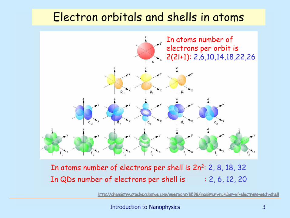
Electron orbitals and shells in atoms

In atoms number of electrons per shell is 2n2: 2, 8, 18, 32

In atoms number of electrons per orbit is 2(2l+1): 2,6,10,14,18,22,26

In QDs number of electrons per shell is : 2, 6, 12, 20

Quantum dots 4

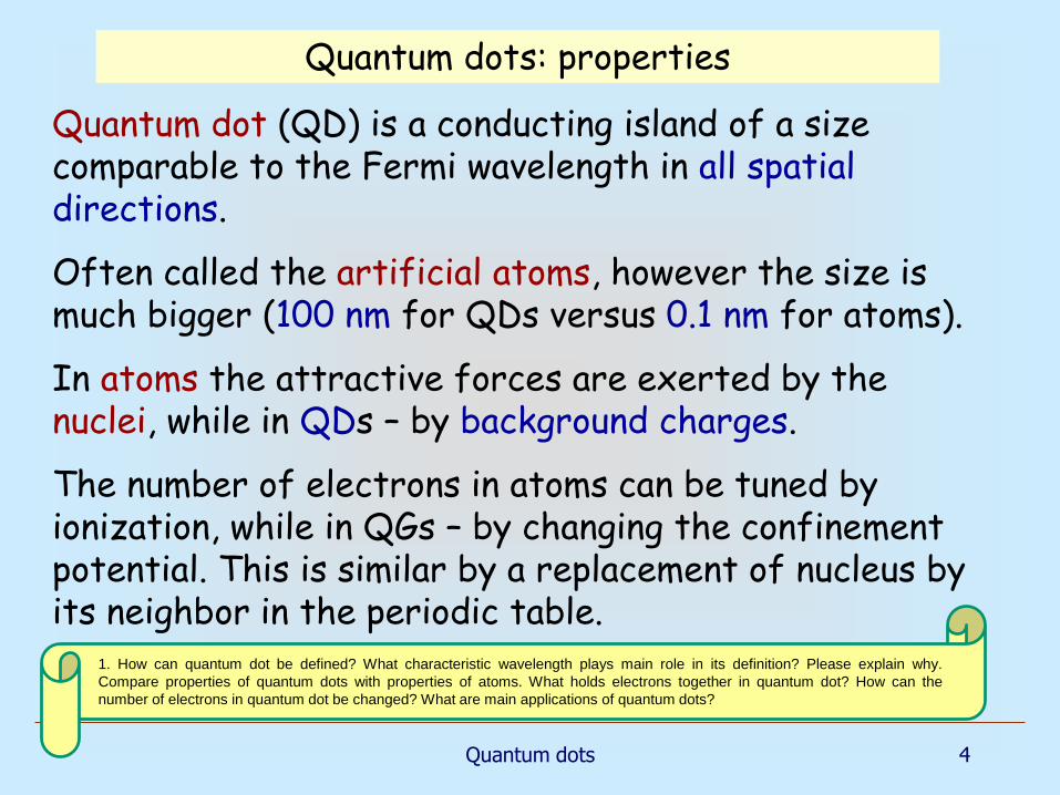
Quantum dot (QD) is a conducting island of a size comparable to the Fermi wavelength in all spatial directions.

Often called the artificial atoms, however the size is much bigger (100 nm for QDs versus 0.1 nm for atoms).

In atoms the attractive forces are exerted by the nuclei, while in QDs – by background charges.

The number of electrons in atoms can be tuned by ionization, while in QGs – by changing the confinement potential. This is similar by a replacement of nucleus by its neighbor in the periodic table.

Quantum dots: properties

1. How can quantum dot be defined? What characteristic wavelength plays main role in its definition? Please explain why.

Compare properties of quantum dots with properties of atoms. What holds electrons together in quantum dot? How can the

number of electrons in quantum dot be changed? What are main applications of quantum dots?

Quantum dots 5

Parameter AtomsQuantum

dots

Level spacing 1 eV 0.1 meV

Ionization energy 10 eV 1 meV

Typical magnetic field to influence

104 T 1-10 T

Comparison between QDs and atoms

QDs are highly tunable. They provide possibilities to place interacting particles into a small volume, allowing to verify fundamental concepts and foster new applications (quantum computing, etc).

Quantum dots 6

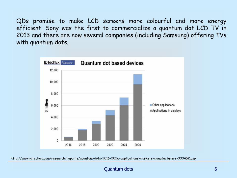
http://www.idtechex.com/research/reports/quantum-dots-2016-2026-applications-markets-manufacturers-000452.asp

QDs promise to make LCD screens more colourful and more energyefficient. Sony was the first to commercialize a quantum dot LCD TV in2013 and there are now several companies (including Samsung) offering TVswith quantum dots.

Introduction 7

Gate

DotElectron

Attraction to the gate

Repulsion at the dot

Cost

Single-electron transistor (SET)

Coulomb blockade in a tunnel barrier

E (Ne) = E ( (N+1)e)

At

the energy cost vanishes !

Q = Ne

Q0 = VgC

Quantum dots 8

QDs and atoms

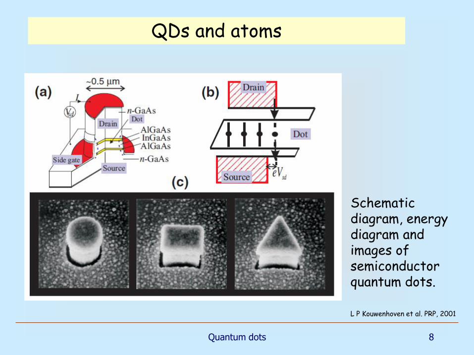
L P Kouwenhoven et al. PRP, 2001

Schematic diagram, energy diagram and images of semiconductor quantum dots.

Quantum dots 9

QDs and atoms: periodic table

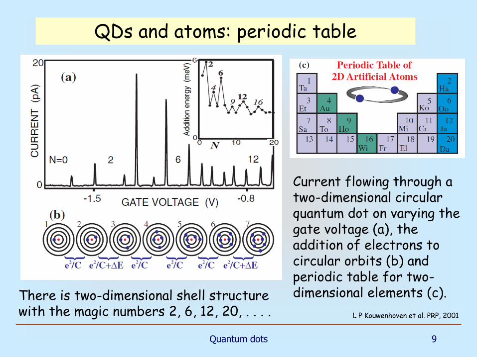
L P Kouwenhoven et al. PRP, 2001

Current flowing through a two-dimensional circular quantum dot on varying the gate voltage (a), the addition of electrons to circular orbits (b) and periodic table for two-dimensional elements (c).There is two-dimensional shell structure

with the magic numbers 2, 6, 12, 20, . . . .

Introduction to Nanophysics 10

Electron orbitals and shells in atoms

In atoms number of electrons per shell is 2n2: 2, 8, 18, 32

In atoms number of electrons per orbit is 2(2l+1): 2,6,10,14,18,22,26

In QDs number of electrons per shell is : 2, 6, 12, 20

Quantum dots 11

AFM micrograph of the gates structure to define a QD in a Ga[Al]As heterostructure.

The Au electrodes (bright) have a height of 100 nm.

The two QPCs formed by the gate pairs F-Q1 and F-Q2

can be tuned into the tunneling regime, such that a QD is formed between the barriers.

Its electrostatic potential can be varied by changing the voltage applied to the center gate

F

Lateral quantum dot

Quantum dots 12

Conductances of all QPCs can be tuned by proper gate voltages.

The F-Q1 and F-Q2 pairs behave as perfect quantized QPCs.

The contact F-C cannot be disconnected, but still shows drop in conductance.

The central gate is designed to couple well to the dot, but with a weak influence on QPCs.

Blue arrow shows the working point.

Lateral quantum dot: conductance

2. Describe lateral quantum dot. What is the conductance as

function of voltage between its different electrodes? How to

disconnect central area of QD from the environment? .

Quantum dots 13

Gate voltage characteristics

The reason of the oscillations was not clear in the beginning:

Coulomb blockade?

Resonant tunneling?

The usual way to find the answer is to study magneto-transport

Pronounced oscillations

3. Oscillations of what parameter are observed in quantum dots

as a function of gate voltage? What could be the nature of these

oscillations? What effects play major role in their appearance?.

Quantum dots 14

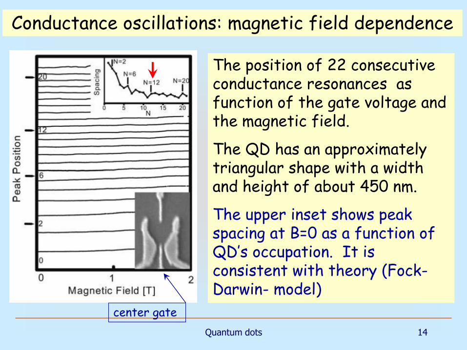
The position of 22 consecutive conductance resonances as function of the gate voltage and the magnetic field.

The QD has an approximately triangular shape with a width and height of about 450 nm.

The upper inset shows peak spacing at B=0 as a function of QD’s occupation. It is consistent with theory (Fock-Darwin- model)

center gate

Conductance oscillations: magnetic field dependence

Quantum dots 15

Why the peaks are not equidistant?

• There is a smooth size dependence on the gate voltage, just because of change in the geometry (and consequently, in capacitances and distance between quantized levels);

• In addition to a smooth dependence there are pronounced fluctuations – a rather rich fine structure.

This fine structure is shown in the next slide, where the smooth part is subtracted

Conductance oscillations: position

Quantum dots 16

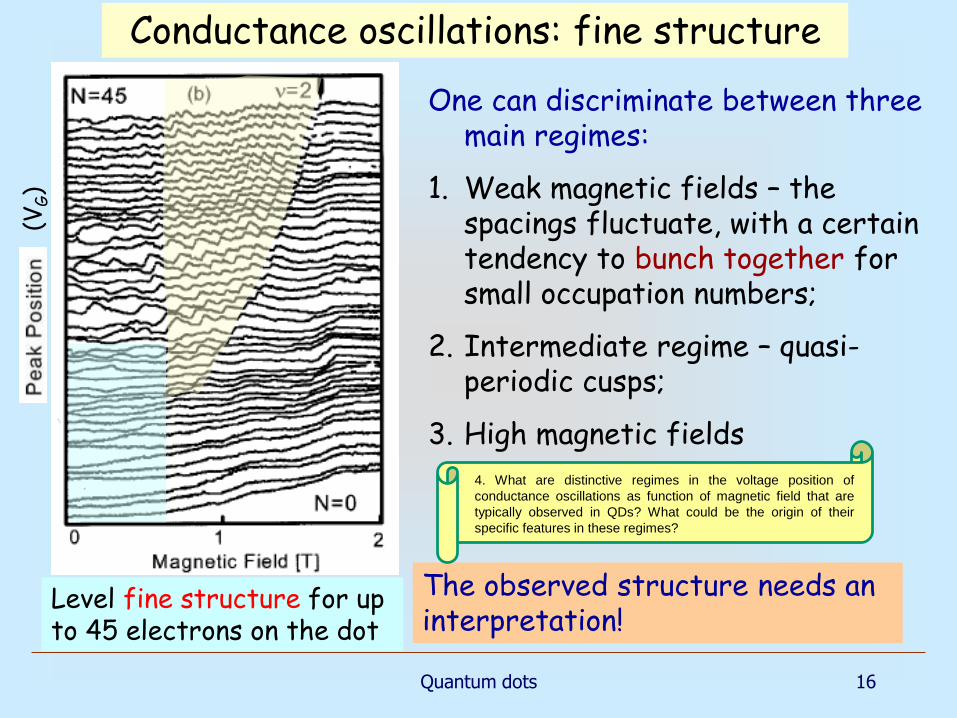
Level fine structure for up to 45 electrons on the dot

One can discriminate between three main regimes:

1. Weak magnetic fields – the spacings fluctuate, with a certain tendency to bunch together for small occupation numbers;

2. Intermediate regime – quasi-periodic cusps;

3. High magnetic fields

The observed structure needs an interpretation!

Conductance oscillations: fine structure(V

G)

4. What are distinctive regimes in the voltage position of

conductance oscillations as function of magnetic field that are

typically observed in QDs? What could be the origin of their

specific features in these regimes?

Quantum dots 17

V=10 μV

What one would expect for a QD device?

Diamond stability diagram

SET

Coulomb blockade oscillations

Quantum dots 18

Stability diagram for a Quantum Dot

Resembles diamond structure for Coulomb blockage (SET) system.

However, size of diamonds fluctuates.

At low bias – resembles usual CB oscillations;

At larger bias a fine structureemerges, which is absent in SETs

5. What is the shape of conductance oscillations in QD? Does it

resemble Coulomb blockage oscillations? Could this effect be

described by the diamond stability diagram for the Coulomb-

blockade single electron transistor? How does amplitude of

oscillations depend on magnetic field?

Quantum dots 19

Finally, the amplitude of resonances can be tuned by magnetic field:

Here we see amplitudes of five consecutive resonances versus magnetic field.

The peak positions fluctuate by about 20% of their spacing, while the amplitude varies by up to 100%.

Plenty of features are waiting for their explanation!

Conductance oscillations: amplitude behaviour

Quantum dots 20

What would follow from the picture of particles with constant interaction?

QD is a zero-dimensional system, its density of states consists of a sequence of peaks, with positions determined by size and shape of the confining potential, as well as by effective mass of the host material.

To estimate the average spacing let us use the 2D model:

This energy should be compared with the typical charging energy, since for an isolated dot the Coulomb blockade must come into play. So we have to develop a way to find the electron addition energy.

The constant interaction (CI) model

Update of solid state physics 21

Number of states per volume per the region k,k+dk

Density of states -Number of states per volume per the

region E,E+dE. Since

3

Density of electron states

Quantum dots 22

Suppose that the highest level in the dot is . Then the next electron will occupy the level having the lowest possible energy.

To find the addition spectrum one has to add this energy to the electrostatic gain, ΔE.

Correspondingly, if we want to remove an electron it is necessary to subtract ,

Adding an electron to a quantum dot

According to the CI model, one assumes that the kinetic energies are independent of the number electrons on the dot, or ΔE and are statistically-independent.

The CI model disregards electron correlations

Quantum dots 23

In general suggesting that kinetic energies are independent of the number electrons on the dot is not correct because of:

• electron–electron interactions

•Screening

•Exchange & correlation effects

Essence of the CI model – adding the difference between kinetic energies to the electrostatic energy cost of addition (removal) of an electron.

The constant interaction model: deficiencies

6. Explain main assumptions of constant interaction (CI) model. Define the distance between the energy levels in 2D quantum dot.

How does it depend on the area of QD? What is other energy scale that is important for CI model? How to calculate the addition

energy of one electron to QD? How to modify single-electron tunnelling model to get CI model? What does constant interaction

model not take into account?

Single electron tunneling 24

The SET transistor

An extra electrode (gate) defined in a way to have very large resistance between it and the island.

That allows to tune induced charges by the gate voltageFulton & Dolan, 1987

The Coulomb gap is given by the onset of the same tunnelling eventsas for the single island studied above. Now, however, the Coulombgap depends upon the gate voltage. The energy differences atelectron tunnelling are:

Coulomb blockade isestablished if all four energydifferences are positive.

Single electron tunneling 25

Stability diagram of Single Electron Transistor (SET)

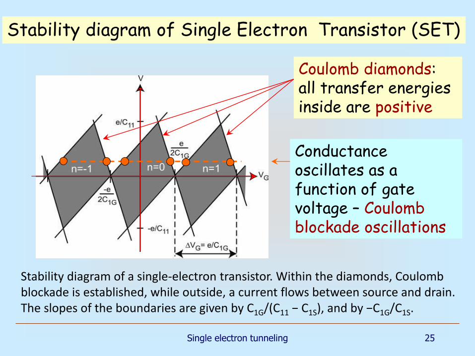
Coulomb diamonds: all transfer energies inside are positive

Conductance oscillates as a function of gate voltage – Coulomb blockade oscillations

Stability diagram of a single-electron transistor. Within the diamonds, Coulomb blockade is established, while outside, a current flows between source and drain. The slopes of the boundaries are given by C1G/(C11 − C1S), and by −C1G/C1S.

Quantum dots 26

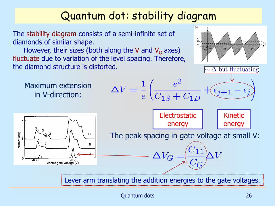
The stability diagram consists of a semi-infinite set of diamonds of similar shape.

However, their sizes (both along the V and VG axes) fluctuate due to variation of the level spacing. Therefore, the diamond structure is distorted.

Maximum extension in V-direction:

Electrostatic energy

Kinetic energy

The peak spacing in gate voltage at small V:

Lever arm translating the addition energies to the gate voltages.

Quantum dot: stability diagram

Quantum dots 27

So far so good, but what should we do with magnetic field?

Analytically solvable model (Fock, Darwin):

Fock-Darwin model

Electron motion is no longer free in the third direction, and the parabolic potential is orientated in the (x, y) plane. The quantum dot is circular in shape and has a parabolic confinement potential.

Quantum dots 28

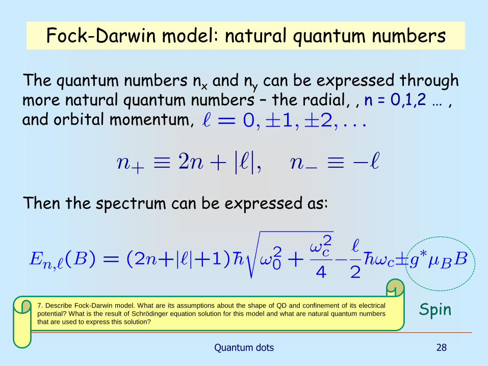
The quantum numbers nx and ny can be expressed through more natural quantum numbers – the radial, , n = 0,1,2 … , and orbital momentum,

Then the spectrum can be expressed as:

Spin

Fock-Darwin model: natural quantum numbers

7. Describe Fock-Darwin model. What are its assumptions about the shape of QD and confinement of its electrical

potential? What is the result of Schrödinger equation solution for this model and what are natural quantum numbers

that are used to express this solution?

Quantum dots 29

At B = 0 the energy levels are just

Magnetic field will remove both orbital and spin degeneracy giving rise to rather complicated spectra.

At B=0 each level has orbital degeneracy ofj+1, in addition, there is a spin degeneracy 2.

Similar to the atomic spectra, we can speak

about jth Darwin-Fock shell.

Filled shells correspond to N=2, 6, 12, 20, ..

Fock-Darwin model: weak magnetic field

8. Introduce the jth Fock–Darwin shell. Illustrate splitting of Fock–Darwin levels by magnetic field. How is it reflected in experimentally

observed behaviour of conductance peaks in low magnetic fields?

Quantum dots 30

The Darwin-Fock spectrum for

Note level crossings!

Predicted evolution of conductance resonance versus gate voltage and magnetic field for

n, l, spin

Fock-Darwin model: splitting of levels

Quantum dots 31

The Darwin-Fock model is a good starting point

– it gives an idea about spectrum in magnetic field

- one can construct filled shells at N=2, 6, 12, 20 …

- it predicts behavior of conductance resonances

However, the agreement with experiment is not prefect

Fock-Darwin model: summary

At B = 0, the energy levels are located at (j + 1)ħω0, with j = 2n + |l|, and with an orbital degeneracy of j+1.

Quantum dots 32

We have explained the low-field part of the curves by the Fock-Darwin model.

Now we have to explain the cusps.

Intermediate magnetic fields

Quantum dots 33

Since in a strong magnetic field confinement is not too important it is reasonable to come back to Landau levels.

Let us define:

Then (spin is neglected)

Intermediate magnetic fields

In large magnetic field the confinement can be neglected and m+1 is just the Landau level number.

Introducing Landau level number

Quantum dots 34

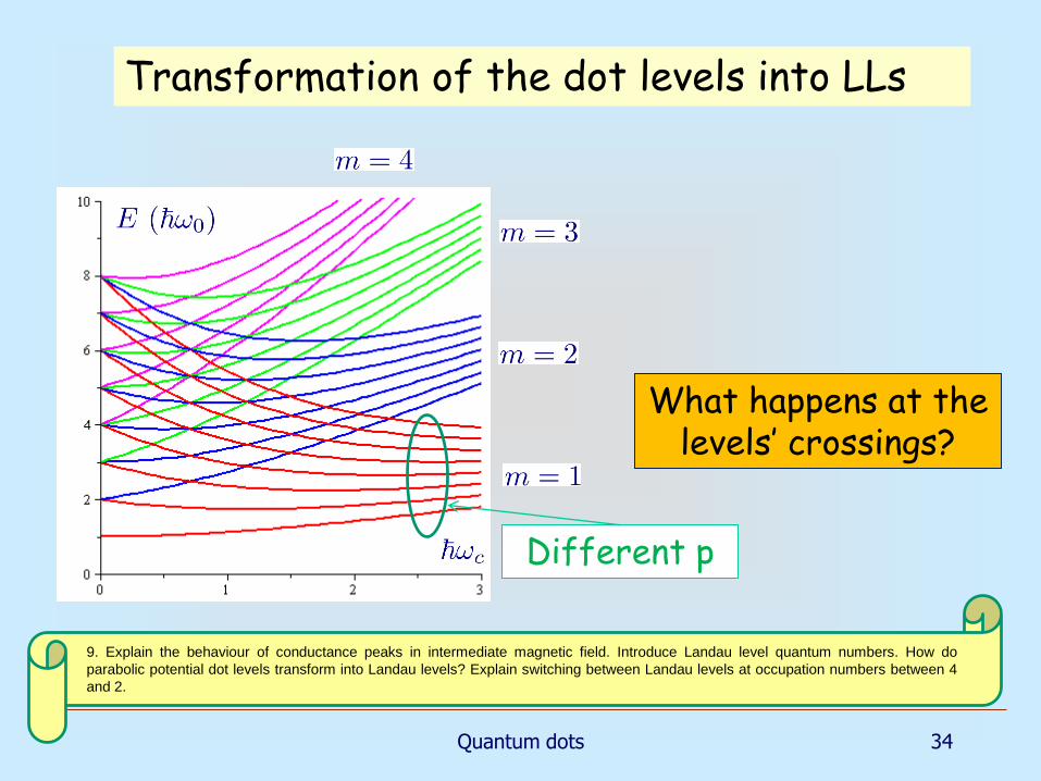
Transformation of the dot levels into LLs

Different p

What happens at the levels’ crossings?

9. Explain the behaviour of conductance peaks in intermediate magnetic field. Introduce Landau level quantum numbers. How do

parabolic potential dot levels transform into Landau levels? Explain switching between Landau levels at occupation numbers between 4

and 2.

Quantum dots 35

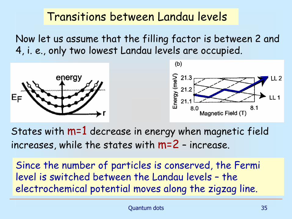
Now let us assume that the filling factor is between 2 and 4, i. e., only two lowest Landau levels are occupied.

States with m=1 decrease in energy when magnetic field

increases, while the states with m=2 – increase.

Since the number of particles is conserved, the Fermi level is switched between the Landau levels – the electrochemical potential moves along the zigzag line.

Transitions between Landau levels

Magnetotransport in 2DEG

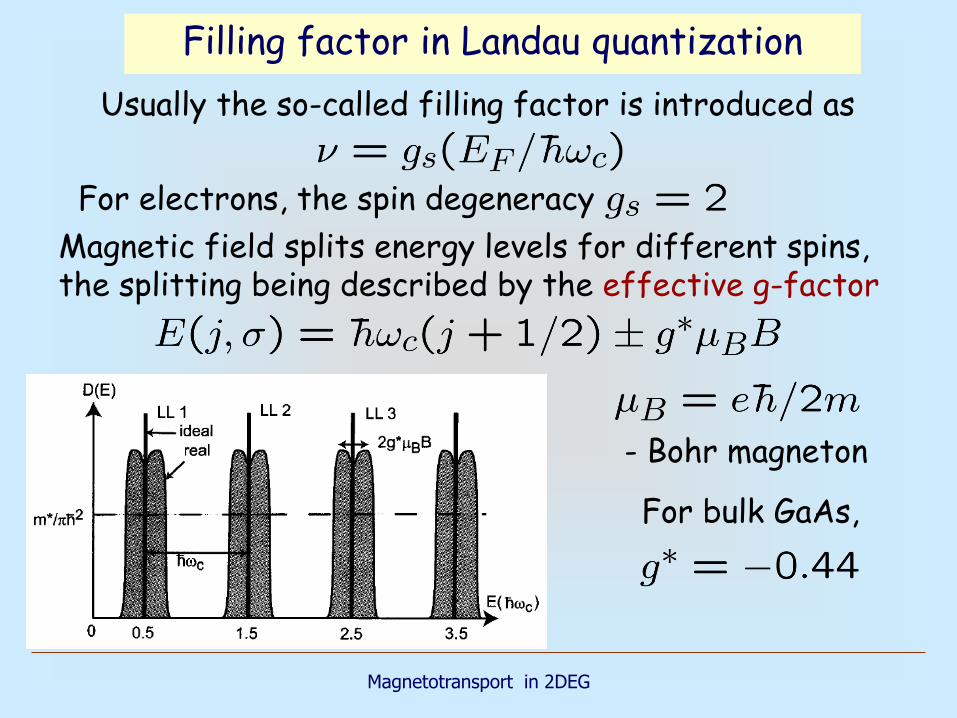
Usually the so-called filling factor is introduced as

For electrons, the spin degeneracy

Magnetic field splits energy levels for different spins, the splitting being described by the effective g-factor

For bulk GaAs,

- Bohr magneton

Filling factor in Landau quantization

Quantum dots 37

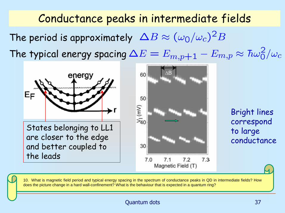
The typical energy spacing

States belonging to LL1 are closer to the edge and better coupled to the leads

Bright lines correspond to large conductance

The period is approximately

Conductance peaks in intermediate fields

10. What is magnetic field period and typical energy spacing in the spectrum of conductance peaks in QD in intermediate fields? How

does the picture change in a hard wall-confinement? What is the behaviour that is expected in a quantum ring?

Quantum dots 38

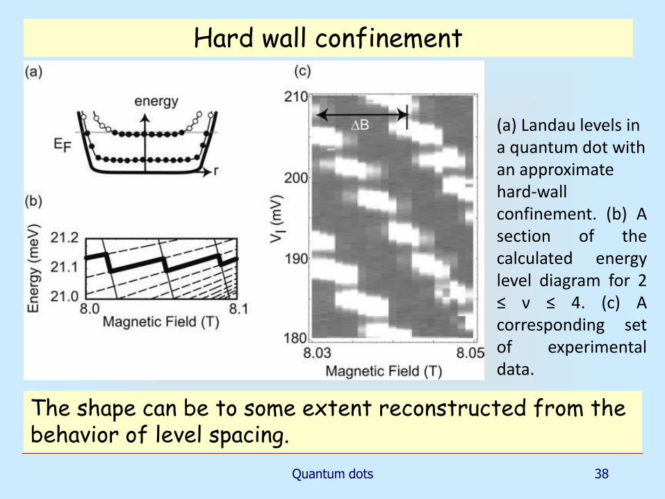
Hard wall confinement

The shape can be to some extent reconstructed from the behavior of level spacing.

(a) Landau levels in a quantum dot with an approximatehard-wallconfinement. (b) Asection of thecalculated energylevel diagram for 2≤ ν ≤ 4. (c) Acorresponding setof experimentaldata.

Quantum dots 39

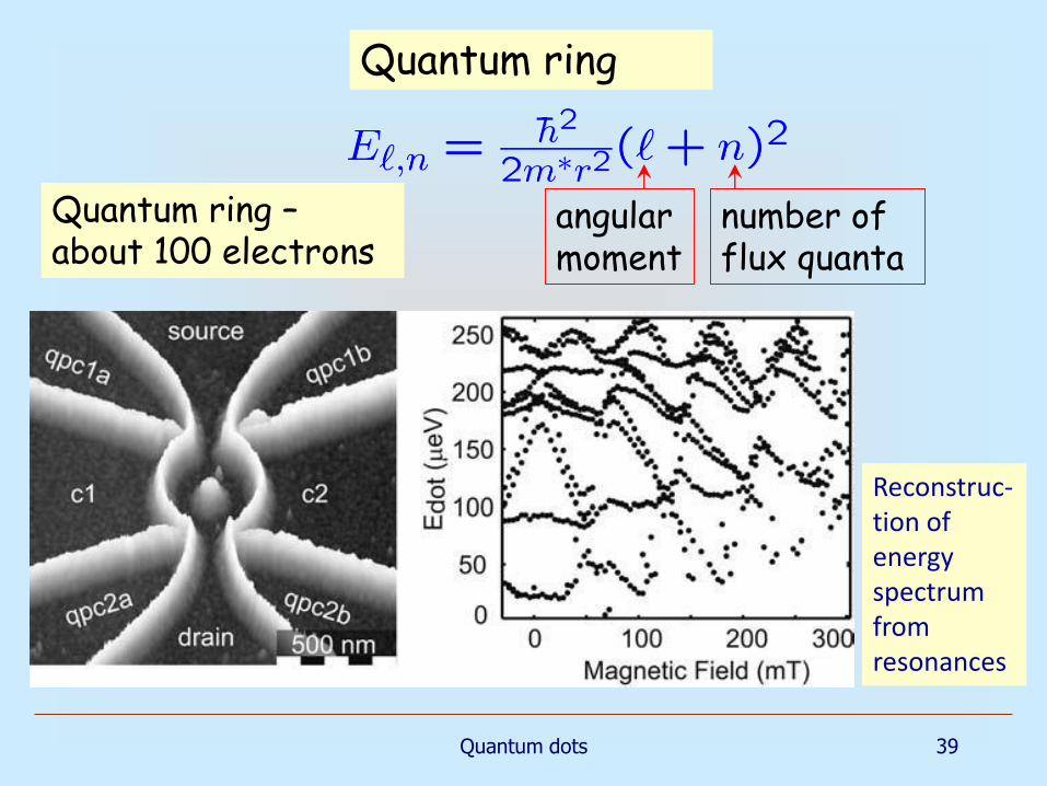
Quantum ring –about 100 electrons

number of flux quanta

angular moment

Reconstruc-tion of energy spectrum from resonances

Quantum ring

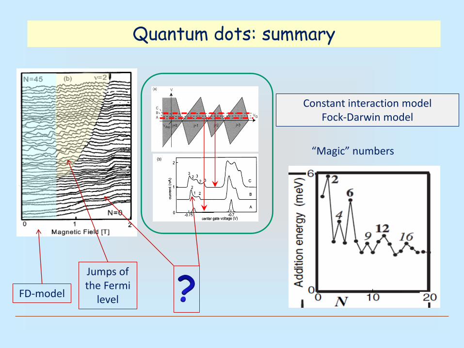
Quantum dots: summary

Constant interaction modelFock-Darwin model

“Magic” numbers

FD-model

Jumps of the Fermi

level

Quantum dots 41

The CI model does not include exchange and correlation effects, such as spin correlations, screening, etc. Here we discuss some of such effects.

Hund’s rules in quantum dots

As known from atomic physics, Hund’s rules determine sequence of the levels’ filling:

1. The total spin gets maximized without violation the Pauli principle (originates in exchange interaction keeping the electrons with parallel spins apart)

2. The orbital angular moment must be maximal keeping restrictions of the rule #1.

3. For a given term, in an atom with outermost subshell half-filled or less, the level with the lowest value of the total angular momentum quantum

number J lies lowest in energy. If the outermost shell is more than half-filled, the level with the highest value of J is lowest in energy.

Beyond the constant interaction model

Quantum dots 42

Filling of the Fock-Darwin potential by first 6 electrons at B = 0.

Configurations are labeled as in atomic physics, 2S+1LJ.

Here S is the spin, J is the total moment, L is the orbital moment. J = L + S.

What happens in strong magnetic field, above the threshold for cusps, i. e. for filling factor below 2?

The CI model even with account of Hund’s rules fails: correlation effects become extremely important.

Hund’s rules in QD

11. Explain Hund’s rules for a quantum dot. How would the filling of the Fock-Darwin potential by first 6 electrons at B = 0 take place?

Are Hund’s rules applicable for filling factor below 2?

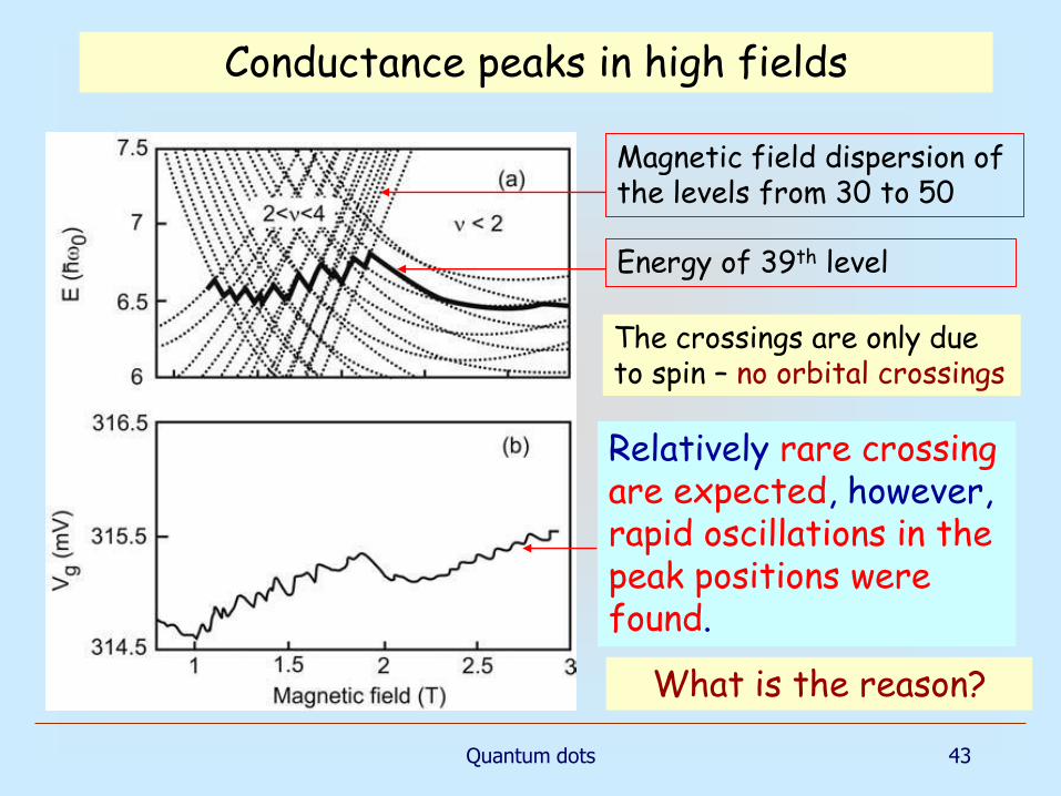
Quantum dots 43

Magnetic field dispersion of the levels from 30 to 50

Energy of 39th level

The crossings are only due to spin – no orbital crossings

Relatively rare crossing are expected, however, rapid oscillations in the peak positions were found.

What is the reason?

Conductance peaks in high fields

Quantum dots 44

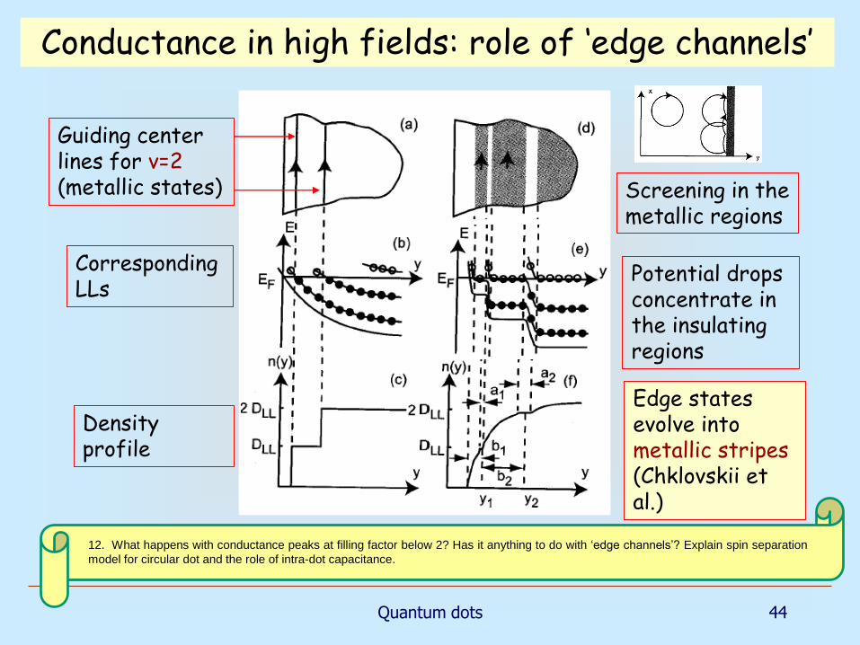
Guiding center lines for ν=2 (metallic states)

Corresponding LLs

Density profile

Screening in the metallic regions

Potential drops concentrate in the insulating regions

Edge states evolve into metallic stripes(Chklovskii et al.)

Conductance in high fields: role of ‘edge channels’

12. What happens with conductance peaks at filling factor below 2? Has it anything to do with ‘edge channels’? Explain spin separation

model for circular dot and the role of intra-dot capacitance.

Quantum dots 45

Phenomenology of circular dot

We arrive at a metallic ring and a disk separated by an insulating ring. The concrete structure depends on effective g-factor.

Now we have to discuss the Coulomb blockade in such system.

The electrostatic cost of the electron transfer between the spin-down and spin-up sublevels should be taken into account. It can be done using an equivalent circuit.

Quantum dots 46

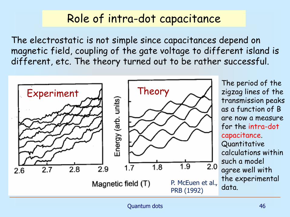
The electrostatic is not simple since capacitances depend on magnetic field, coupling of the gate voltage to different island is different, etc. The theory turned out to be rather successful.

Experiment Theory

P. McEuen et al., PRB (1992)

The period of the zigzag lines of thetransmission peaks as a function of B are now a measure for the intra-dot capacitance. Quantitative calculations within such a model agree well with the experimental data.

Role of intra-dot capacitance

Quantum dots 47

Thus we arrive at the following summary:

• In weak magnetic field Fock-Darwin model allows for the conductance resonances;

• In intermediate magnetic fields the field-induced repopulation of LLs becomes crucially important;

• In strong magnetic field the CI model fails, and correlation effects become important. The most important are spincorrelations in combination with screening effects.

Quantum dot behaviour

Quantum dots 48

Quasi-chaotic

The upper levels depend on magnetic field in a quasi-chaotic fashion.Sometimes people call such a behavior the quantized chaos.

Quasi-chaotic behaviour

13. Does quasi-chaotic behaviour take place in quantum dots? If yes, how is it

expressed? Is it classical or quantum chaos? What is the difference?

Quantum dots 49

At large occupation numbers and in weak magnetic fields many levels are involved, and the energy spectrum becomes very complicated.

Is any way to find universal properties avoiding concrete energy spectrum?

The proper theory is referred to as quantized chaos.The classical system is called chaotic if its evolution in time depends exponentially on changes of the initial conditions.

Example - a particle in the box, classical dynamics with specular reflection.

The trajectory depends on the initial condition, p(0) and r(0).

The distribution of nearest neighbor spacing

Quantum dots 50

Let us discuss how the difference between 2 trajectories,

evolves in time for the time much larger then the elementary traversal time provided the position difference at the initial time is infinitesimally small.

The answer strongly depends on the shape of the cavity. If it diverges exponentially, then the cavity is called chaotic. Otherwise it is called regular.

Most shapes – like the Sinai billiard –show chaotic dynamics.

Quantization of chaotic dynamics is a tricky business

Chaos in classical and quantum systems

Quantum dots 51

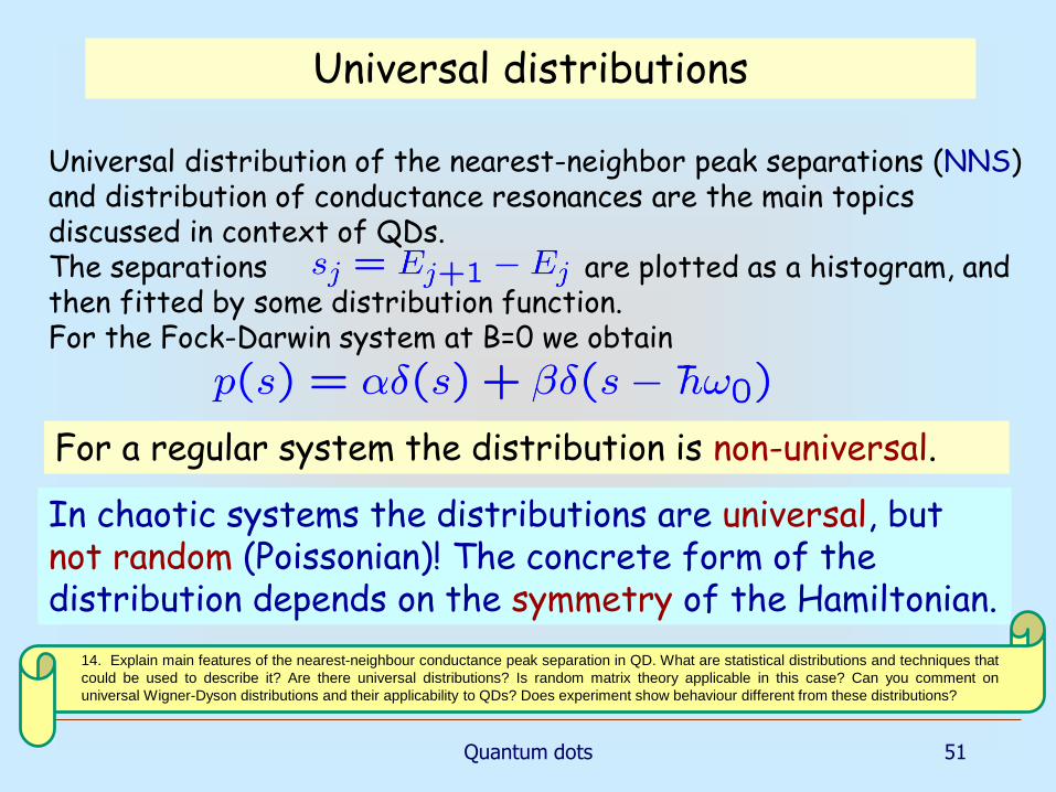
Universal distribution of the nearest-neighbor peak separations (NNS) and distribution of conductance resonances are the main topics discussed in context of QDs.The separations are plotted as a histogram, and then fitted by some distribution function.For the Fock-Darwin system at B=0 we obtain

For a regular system the distribution is non-universal.

In chaotic systems the distributions are universal, but not random (Poissonian)! The concrete form of the distribution depends on the symmetry of the Hamiltonian.

Universal distributions

14. Explain main features of the nearest-neighbour conductance peak separation in QD. What are statistical distributions and techniques that

could be used to describe it? Are there universal distributions? Is random matrix theory applicable in this case? Can you comment on

universal Wigner-Dyson distributions and their applicability to QDs? Does experiment show behaviour different from these distributions?

Quantum dots 52

Random matrix theory

Hamiltonian is presented as a matrix in some basis, the matrix elements being assumed random, but satisfying symmetry requirements.

If the Hamiltonian is invariant with respect to time inversion, then the matrix should be orthogonal.

If time reversal symmetry is broken, then the matrix is unitary.

These two cases are called the Gaussian orthogonal ensemble (GOE) and Gaussian unitary ensemble (GUE), respectively.

Quantum dots 53

The results of rather complicated analysis shows that these cases are covered by universal Wigner-Dyson distributions.

With spin-degeneracy

Wigner surmises: two level system distributions

Quantum dots 54

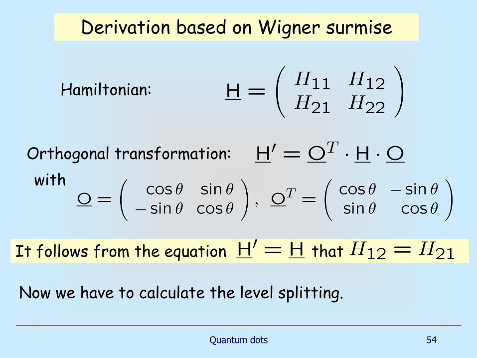
Derivation based on Wigner surmise

Hamiltonian:

Orthogonal transformation:

with

It follows from the equation that

Now we have to calculate the level splitting.

Quantum dots 55

Eigenvalues (in general):

Splitting:

Eigenvalues and splitting

Quantum dots 56

It is assumed here that p1 and p2 are smooth functions.

From the invariance with respect to unitarytransformation one would get

Then there are three independent variables, Δ and h1=Re h, h2=Im h.

Δ

h

s

Derivation

Quantum dots 57

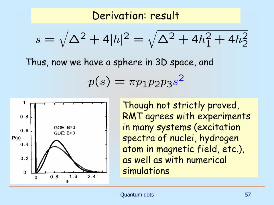
Thus, now we have a sphere in 3D space, and

Though not strictly proved, RMT agrees with experiments in many systems (excitation spectra of nuclei, hydrogen atom in magnetic field, etc.), as well as with numerical simulations

Derivation: result

Quantum dots 58

An example of numerical calculations for Sinai billiard (about 1000 eigenvalues) –histogram.

Comparison with GOE Wigner surmise and Poisson distribution is also shown

NNS distributions “know” whether the states are extended or localized.

This property is extensively used in numerical studies of localization.

Universal distributions

Quantum dots 59

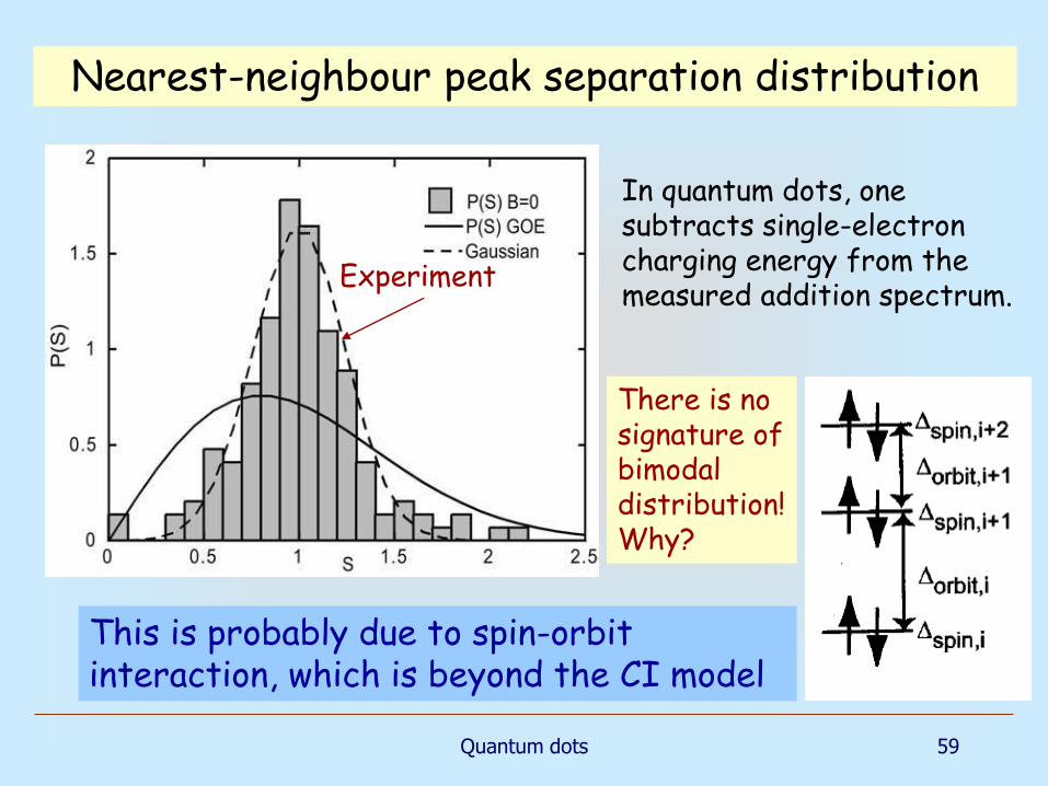
In quantum dots, one subtracts single-electron charging energy from the measured addition spectrum.

There is no signature of bimodal distribution! Why?

This is probably due to spin-orbit interaction, which is beyond the CI model

Experiment

Nearest-neighbour peak separation distribution

Quantum dots 60

Studies of nearest-neighbor peak separation distributions is a powerful tool for optimizing various model for residual interactions in small systems.

This area is still under development.

NNS distribution summary

Quantum dots 61

Earlier we discussed only the information emerging from peak positions.

What can be found form the amplitude and shape of conductance resonances?

Clearly, the peak shape and amplitude depend on the coupling to the leads. This fact can be used to find the properties of the wave functions.

This is in contrast to SET where many states are coupled to the leads and the peak amplitudes are almost constant.

Amplitude and shape of conductance resonances

15. What are approaches that could be taken to explain amplitude and shape of conductance resonances? Can you explain amplitude

variation in a simple diagram model of quantised levels for a QD separated by two tunnelling barriers? What is the role of electrostatic

charging energy there? How can single-particle levels be determined by high-bias transport measurements? Can shape of resonances be

easily analysed?

Quantum dots 62

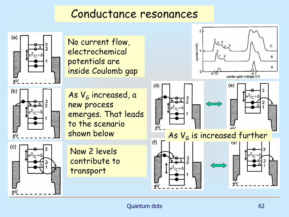
Conductance resonances

No current flow, electrochemical potentials are inside Coulomb gap

As VG increased, a new process emerges. That leads to the scenario shown below

Now 2 levels contribute to transport

As VG is increased further

Quantum dots 63

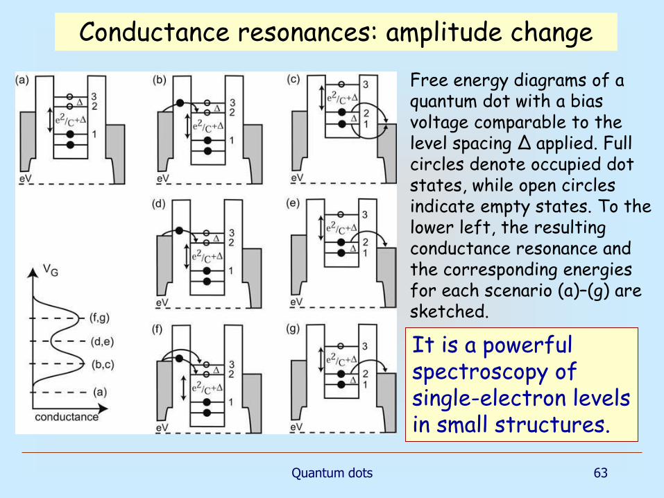
It is a powerful spectroscopy of single-electron levels in small structures.

Free energy diagrams of a quantum dot with a bias voltage comparable to the level spacing Δ applied. Full circles denote occupied dot states, while open circles indicate empty states. To the lower left, the resulting conductance resonance and the corresponding energies for each scenario (a)–(g) are sketched.

Conductance resonances: amplitude change

Quantum dots 64

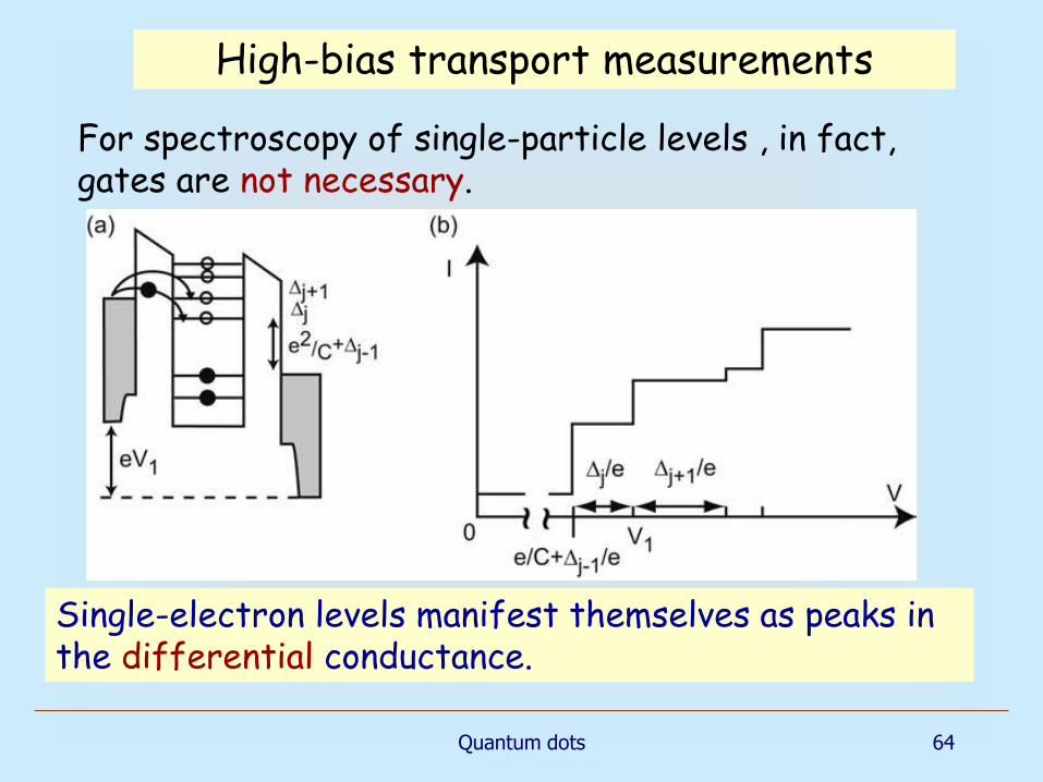
For spectroscopy of single-particle levels , in fact, gates are not necessary.

Single-electron levels manifest themselves as peaks in the differential conductance.

High-bias transport measurements

Quantum dots 65

Shape of resonances

This is a complicated problem since all important

parameters – kBΘ, Δ, and hΓ - are usually of the same order of magnitude.

No analytical expression for the shape in general case since

•Coulomb correlation of tunneling through different barriers;

•Electron distribution function inside the dot is non-equilibrium

Quantum dots 66

Quantum dots 67

On-surface fabrication of graphene

quantum dots. (a) Schematic

illustration of the formation of a 14-

AGNR quantum dot by edge fusion of

two 7-AGNRs. (b) STM image showing

several 7-14-7 quantum dot

heterostructures on Au(111). Scale bar:

5 nm. (c) nc-AFM frequency shift

image of a long 14-AGNR segment

acquired with a CO functionalized tip.

Scale bar: 2 nm. (d) nc-AFM image of

a short 7-14-7 AGNR quantum dot.

Scale bar: 2 nm. (e) Schematic energy

level diagram of the 7-14-7 AGNR

quantum dot in (d). Two red lines

indicate a pair of low-energy interface

states, and the black lines indicate the

levels arising from longitudinal

quantum confinement of

electrons/holes within the 14-AGNR

quantum dot segment.

Quantum dots 68

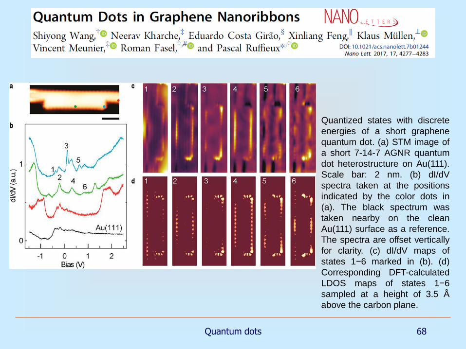
Quantized states with discrete

energies of a short graphene

quantum dot. (a) STM image of

a short 7-14-7 AGNR quantum

dot heterostructure on Au(111).

Scale bar: 2 nm. (b) dI/dV

spectra taken at the positions

indicated by the color dots in

(a). The black spectrum was

taken nearby on the clean

Au(111) surface as a reference.

The spectra are offset vertically

for clarity. (c) dI/dV maps of

states 1−6 marked in (b). (d)

Corresponding DFT-calculated

LDOS maps of states 1−6

sampled at a height of 3.5 Å

above the carbon plane.

Quantum dots 69

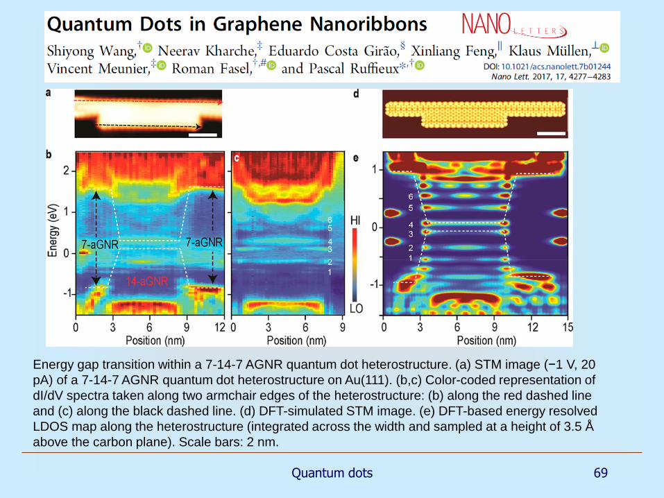
Energy gap transition within a 7-14-7 AGNR quantum dot heterostructure. (a) STM image (−1 V, 20

pA) of a 7-14-7 AGNR quantum dot heterostructure on Au(111). (b,c) Color-coded representation of

dI/dV spectra taken along two armchair edges of the heterostructure: (b) along the red dashed line

and (c) along the black dashed line. (d) DFT-simulated STM image. (e) DFT-based energy resolved

LDOS map along the heterostructure (integrated across the width and sampled at a height of 3.5 Å

above the carbon plane). Scale bars: 2 nm.

Quantum dots 70

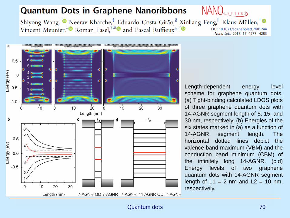
Length-dependent energy level

scheme for graphene quantum dots.

(a) Tight-binding calculated LDOS plots

of three graphene quantum dots with

14-AGNR segment length of 5, 15, and

30 nm, respectively. (b) Energies of the

six states marked in (a) as a function of

14-AGNR segment length. The

horizontal dotted lines depict the

valence band maximum (VBM) and the

conduction band minimum (CBM) of

the infinitely long 14-AGNR. (c,d)

Energy levels of two graphene

quantum dots with 14-AGNR segment

length of L1 = 2 nm and L2 = 10 nm,

respectively.

Quantum dots 71

Vertical dots

Granular materialsMO composites:Encapsulated 4 nm Au particles self-assembled into a 2D array

Surface clustersIndividual grains

Nano-pendulum

Other types of quantum dots

Quantum dots 72

Components of molecular electronics

Self-assembled

arrays

Ge-in-Si

Hybrid structure for CNOT quantum gate

Other QDs and molecular electronics

16. Give examples of other than semiconducting quantum dots. Could

they be used as components of molecular electronics? Can nano-crystals

be used as QD? Can you give examples of these?

Quantum dots 73

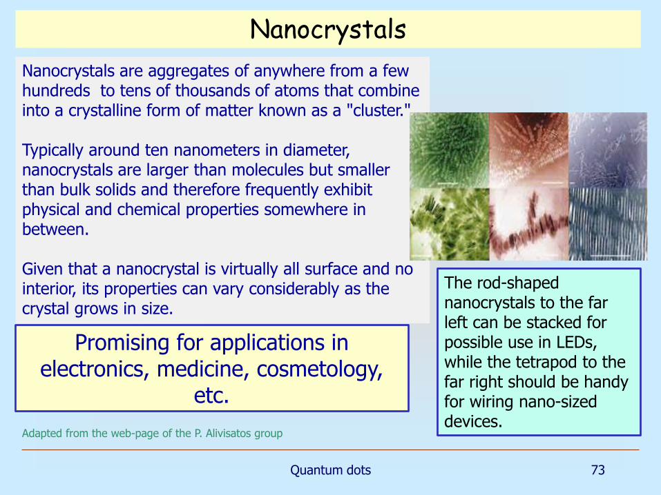
Nanocrystals

Nanocrystals are aggregates of anywhere from a few hundreds to tens of thousands of atoms that combine into a crystalline form of matter known as a "cluster."

Typically around ten nanometers in diameter, nanocrystals are larger than molecules but smaller than bulk solids and therefore frequently exhibit physical and chemical properties somewhere in between.

Given that a nanocrystal is virtually all surface and no interior, its properties can vary considerably as the crystal grows in size.

The rod-shaped nanocrystals to the far left can be stacked for possible use in LEDs, while the tetrapod to the far right should be handy for wiring nano-sized devices.

Promising for applications in electronics, medicine, cosmetology,

etc.

Adapted from the web-page of the P. Alivisatos group

Quantum dots 74

Quantum dots are main ingredients of modern and future nanoscience and nanotechnology.

There was a substantial progress in their studies, many properties are already understood.

However, many issues, in particular, role of electron-electron orbital and spin correlations, remain to be fully understood.

This is a very exciting research area.

Summary