
Quantum Control1 International Graduate School on Control ...
172
Quantum Control 1 International Graduate School on Control www.eeci-igsc.eu Pierre Rouchon 2 Lecture 1 Chengdu, July 8, 2019 1 An important part of these slides gathered at the following web page have been elaborated with Mazyar Mirrahimi: http://cas.ensmp.fr/~rouchon/ChengduJuly2019/index.html 2 Mines ParisTech, INRIA Paris
Transcript of Quantum Control1 International Graduate School on Control ...

Quantum Control1
International Graduate School on Controlwww.eeci-igsc.eu
Pierre Rouchon2
Lecture 1Chengdu, July 8, 2019
1An important part of these slides gathered at the following web pagehave been elaborated with Mazyar Mirrahimi:http://cas.ensmp.fr/~rouchon/ChengduJuly2019/index.html
2Mines ParisTech, INRIA Paris

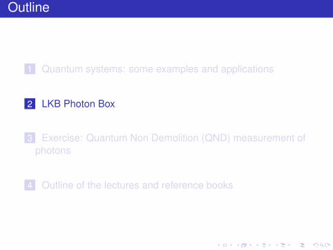
Outline
1 Quantum systems: some examples and applications
2 LKB Photon Box
3 Exercise: Quantum Non Demolition (QND) measurement ofphotons
4 Outline of the lectures and reference books

Controlling quantum degrees of freedom
Some applications
Nuclear Magnetic Resonance (NMR) applications;
Quantum chemical synthesis;
High resolution measurement devices (e.g. atomic/optic clocks);
Quantum communication;
Quantum computation .
Physics Nobel prize 2012
Serge Haroche David J. Wineland Nobel prize: ground-breaking experimental methods that enable measuring
and manipulation of individual quantum systems.

Technologies for quantum simulation and computation3
© OBrien
Superconducngcircuits
Photons
© S. Kuhr
Ultra-cold neutral/Rydberg
atoms
© Bla & Wineland
Trapped ions
© Pea
Quantum dots
© IBM
Requirement:Scalable modular architectureControl software from the very beginning.
3Courtesy of Walter Riess, IBM Research - Zurich.

Quantum computation: towards quantum electronics
D-Wave machine: machines to solve certain huge-dimensional optimizationproblems (state space of dimension 2100).
Major challenge: Fragility of quantum information versus external noise.
Quantum error correction
We protect quantum information by stabilizing a manifold of quantum states.
Outline
1 Quantum systems: some examples and applications
2 LKB Photon Box
3 Exercise: Quantum Non Demolition (QND) measurement ofphotons
4 Outline of the lectures and reference books

The LKB Photon box 4
The first experimental realization of a quantum-state feedback:
Theory: I. Dotsenko, . . . : Quantum feedback by discrete quantumnon-demolition measurements: towards on-demand generation ofphoton-number states. Physical Review A, 2009, 80: 013805-013813.Experiment: C. Sayrin, . . . , S. Haroche:Real-time quantum feedback prepares and stabilizes photon numberstates. Nature, 2011, 477, 73-77.
4Laboratoire Kastler-Brossel (LKB), http://www.lkb.upmc.fr/cqed/

Three quantum features emphasized by the LKB photon box 5
1 Schrödinger (~ = 1): wave function |ψ〉 in Hilbert space H,
ddt|ψ〉 = −iH|ψ〉, H = H0 + uH1.
Unitary propagator U solution of ddt U = −iHU with U(0) = I.
2 Origin of dissipation: collapse of the wave packet induced by themeasurement of observable O with spectral decomp.
∑µ λµPµ:
measurement outcome µ with proba. Pµ = 〈ψ|Pµ|ψ〉 dependingon |ψ〉, just before the measurementmeasurement back-action if outcome µ = y :
|ψ〉 7→ |ψ〉+ =Py |ψ〉√〈ψ|Py |ψ〉
3 Tensor product for the description of composite systems (S,M):Hilbert space H = HS ⊗HM
Hamiltonian H = HS ⊗ IM + H int + IS ⊗ HM
observable on sub-system M only: O = IS ⊗OM .
5S. Haroche and J.M. Raimond. Exploring the Quantum: Atoms, Cavitiesand Photons. Oxford Graduate Texts, 2006.

Composite system (S,M): harmonic oscillator ⊗ qubit.
System S corresponds to a quantized harmonic oscillator:
HS =
∞∑n=0
ψn |n〉∣∣∣∣ (ψn)∞n=0 ∈ l2(C)
,
where |n〉 is the photon-number state with n photons(〈n1|n2〉 = δn1,n2 ).Meter M is a qubit, a 2-level system:
HM =
ψg |g〉+ ψe|e〉
∣∣∣∣ ψg , ψe ∈ C,
where |g〉 (resp. |e〉) is the ground (resp. excited) state(〈g|g〉 = 〈e|e〉 = 1 and 〈g|e〉 = 0)State of the composite system |Ψ〉 ∈ HS ⊗HM :
|Ψ〉 =∑n≥0
(Ψng |n〉 ⊗ |g〉+ Ψne |n〉 ⊗ |e〉
)=
∑n≥0
Ψng |n〉
⊗ |g〉+
∑n≥0
Ψne |n〉
⊗ |e〉, Ψne,Ψng ∈ C.
Ortho-normal basis:(|n〉 ⊗ |g〉, |n〉 ⊗ |e〉
)n∈N.

Quantum trajectories (1)
C
B
D
R 1R 2
B R 2
When atom comes out B, the quantum state |Ψ〉B of thecomposite system is separable: |Ψ〉B = |ψ〉 ⊗ |g〉.
Just before the measurement in D, the state is in generalentangled (not separable):
|Ψ〉R2= USM
(|ψ〉 ⊗ |g〉
)=(Mg |ψ〉
)⊗ |g〉+
(Me|ψ〉
)⊗ |e〉
where USM = UR2UCUR1 is a unitary transformation(Schrödinger propagator) defining the measurement operatorsMg and Me on HS. Since USM is unitary, M†gMg + M†eMe = I .

Quantum trajectories (2)
Just before detector D the quantum state is entangled:
|Ψ〉R2= (Mg |ψ〉)⊗ |g〉+ (Me|ψ〉)⊗ |e〉
Just after outcome y , the state becomes separable 6:
|Ψ〉D =
My√⟨ψ|M†
y My |ψ⟩ |ψ〉
⊗ |y〉.Outcome y obtained with probability Py =
⟨ψ|M†y My |ψ
⟩..
Quantum trajectories (Markov chain, stochastic dynamics):
|ψk+1〉 =
Mg√⟨
ψk |M†g Mg |ψk
⟩ |ψk 〉, yk = g with probability⟨ψk |M†gMg |ψk
⟩;
Me√⟨ψk |M
†e Me|ψk
⟩ |ψk 〉, yk = e with probability⟨ψk |M†eMe|ψk
⟩;
with state |ψk 〉 and measurement outcome yk ∈ g, e at time-step k :
6Measurement operator O = IS ⊗ (|e〉〈e| − |g〉〈g|).

Exercise: Quantum Non Demolition (QND) measurement of photons 7
Goal |Ψ〉R2= UR2 UCUR1
(|ψ〉 ⊗ |g〉
)=?
C
B
D
R 1R 2
B R 2
UR1 = IS ⊗((|g〉+|e〉√
2
)〈g|+
(|g〉−|e〉√
2
)〈e|
)UC = e−i
φ02 N ⊗ |g〉〈g|+ ei
φ02 N ⊗ |e〉〈e|
where N|n〉 = n|n〉, ∀n ∈ N and φ0 ∈ R.
UR2 = UR1
1 Show that UR1
(|ψ〉 ⊗ |g〉
)= 1√
2(|ψ〉 ⊗ |g〉+ |ψ〉 ⊗ |e〉) and
UCUR1
(|ψ〉 ⊗ |g〉
)= 1√
2
((e−i
φ02 N |ψ〉
)⊗ |g〉+
(eiφ02 N |ψ〉
)⊗ |e〉
).
2 Show that |Ψ〉R2=
(cos(φ0
2 N)|ψ〉)⊗ |g〉+
(i sin(φ0
2 N)|ψ〉)⊗ |e〉
3 Deduce that Mg = cos(φ02 N) and Me = −i sin(φ0
2 N).
4 Question for Wednesday: write a computer program (e.g. a Scilab or Matlabscript) to simulate over 20 sampling steps the attached Markov chain startingfrom |ψ0〉 = 1√
2(|0〉+ |1〉) with parameter φ0 = π/3 (Quantum Monte-Carlo
trajectories).
7M. Brune, . . . : Manipulation of photons in a cavity by dispersive atom-fieldcoupling: quantum non-demolition measurements and generation of "Schrödinger cat"states . Physical Review A, 45:5193-5214, 1992.

Outline
1 Quantum systems: some examples and applications
2 LKB Photon Box
3 Exercise: Quantum Non Demolition (QND) measurement ofphotons
4 Outline of the lectures and reference books

Outline of the lectures
Monday 1- Introduction (motivating applications; LKB photon-box as prototype of openquantum system). 2- Spring system (harmonic oscillator, spectraldecomposition, annihilation/creation operators, coherent state anddisplacement). 3- Spin system (qubit, Pauli matrices). 4- Composite spin/springsystem (tensor product, resonant/dispersive interaction, underlying PDE’s).
Tuesday 5- Averaging and rotating waves approximation (first/second order perturbationexpansion,) 6-Open-loop control via averaging techniques (resonant control forqubit and Jaynes-Cummings systems)
Wednesday 7- Discrete-time dynamics of the LKB photon box (density operators,measurement imperfection, decoherence, quantum filter) 8- Discrete-timeStochastic Master Equation (SME) (Positive Operator Value Measurement(POVM), Kraus maps and quantum channels, stability and contractions,Schrödinger and Heisenberg points of view). 9- Discrete-time Quantum NonDemolition (QND) measurement (martingales, convergence of Markovprocesses, Kushner invariance Theorem) 10- Measurement-based feedback andLyapunov stabilization of photons (LKB photon box with dispersive/resonnantprobe atoms, closed-loop Monte-Carlo simulations).
Thursday 11- Continuous-time Stochastic Master Equation (SME) (Wiener processes andIto calculus, continuous-time measurement, quantum filtering) 12-Measurement-based feedback stabilization of a qubit (Lyapunov feedback,closed-loop Monte-Carlo simulations)
Friday 13- Lindblad master equation (decoherence models for a qubit and an oscillator )14- Coherent-feedback stabilization (principle, cat-qubit and multi-photonpumping)

Reference books
1 Cohen-Tannoudji, C.; Diu, B. & Laloë, F.: Mécanique Quantique Hermann, Paris,1977, I& II (quantum physics: a well known and tutorial textbook)
2 S. Haroche, J.M. Raimond: Exploring the Quantum: Atoms, Cavities andPhotons. Oxford University Press, 2006. (quantum physics: spin/spring systems,decoherence, Schrödinger cats, entanglement. )
3 C. Gardiner, P. Zoller: The Quantum World of Ultra-Cold Atoms and Light I& II.Imperial College Press, 2009. (quantum physics, measurement and control)
4 Barnett, S. M. & Radmore, P. M.: Methods in Theoretical Quantum Optics OxfordUniversity Press, 2003. (mathematical physics: many useful operator formulaefor spin/spring systems )
5 E. Davies: Quantum Theory of Open Systems. Academic Press, 1976.(mathematical physics: functional analysis aspects when the Hilbert space is ofinfinite dimension )
6 Gardiner, C. W.: Handbook of Stochastic Methods for Physics, Chemistry, andthe Natural Sciences [3rd ed], Springer, 2004. (tutorial introduction to probability,Markov processes, stochastic differential equations and Ito calculus. )
7 M. Nielsen, I. Chuang: Quantum Computation and Quantum Information.Cambridge University Press, 2000. (tutorial introduction with a computer scienceand communication view point )

Quantum Control1
International Graduate School on Controlwww.eeci-igsc.eu
Pierre Rouchon2
Lecture 2Chengdu, July 8, 2019
1An important part of these slides gathered at the following web pagehave been elaborated with Mazyar Mirrahimi:http://cas.ensmp.fr/~rouchon/ChengduJuly2019/index.html
2Mines ParisTech, INRIA Paris

Outline
1 Quantum harmonic oscillator: spring model
2 Summary of main formulae
3 Exercise: useful operator identities

Outline
1 Quantum harmonic oscillator: spring model
2 Summary of main formulae
3 Exercise: useful operator identities

Harmonic oscillator
Classical Hamiltonian formulation of d2
dt2 x = −ω2x
ddt
x = ωp =∂H∂p
,ddt
p = −ωx = −∂H∂x
, H =ω
2(p2 + x2).
Mechanical oscillator
Frictionless spring: d2
dt2 x = − km x .
Electrical oscillator:
L C
I+
−
V
LC oscillator:
ddt
I =VL,
ddt
V = − IC, (
d2
dt2 I = − 1LC
I).
Quantum regime
kBT ~ω : typically for the photon box experiment in these lectures,ω = 51GHz and T = 0.8K .

Harmonic oscillator3: quantization and correspondence principleddt x = ωp = ∂H
∂p ,ddt p = −ωx = −∂H
∂x , H = ω2 (p
2 + x2).
Quantization: probability wave function |ψ〉t ∼ (ψ(x , t))x∈R with|ψ〉t ∼ ψ( , t) ∈ L2(R,C) obeys to the Schrödinger equation(~ = 1 in all the lectures)
iddt|ψ〉 = H|ψ〉, H = ω(P2 + X 2) = −ω
2∂2
∂x2 +ω
2x2
where H results from H by replacing x by position operator√2X and p by momentum operator
√2P = −i ∂∂x . H is a
Hermitian operator on L2(R,C), with its domain to be given.
PDE model: i ∂ψ∂t (x , t) = −ω2∂2ψ∂x2 (x , t) + ω
2 x2ψ(x , t), x ∈ R.
3Two references: C. Cohen-Tannoudji, B. Diu, and F. Laloë. MécaniqueQuantique, volume I& II. Hermann, Paris, 1977.M. Barnett and P. M. Radmore. Methods in Theoretical Quantum Optics.Oxford University Press, 2003.

Harmonic oscillator: annihilation and creation operators
Average position 〈X 〉t = 〈ψ|X |ψ〉 and momentum 〈P〉t = 〈ψ|P|ψ〉:
〈X 〉t = 1√2
∫ +∞
−∞x |ψ|2dx , , 〈P〉t = − i√
2
∫ +∞
−∞ψ∗∂ψ
∂xdx .
Annihilation a and creation operators a† (domains to be given):
a = X + iP = 1√2
(x +
∂
∂x
), a† = X − iP = 1√
2
(x − ∂
∂x
)Commutation relationships:
[X ,P] = i2 I , [a,a†] = I , H = ω(P2 + X 2) = ω
(a†a +
I2
).

Harmonic oscillator: spectral decomposition and Fock states
Spectrum of Hamiltonian H = −ω2 ∂2
∂x2 + ω2 x2 :
En = ω(n+12), ψn(x) =
(1π
)1/4 1√2nn!
e−x2/2Hn(x), Hn(x) = (−1)nex2 dn
dxn e−x2.
Spectral decomposition of a†a using [a,a†] = 1:
If |ψ〉 is an eigenstate associated to eigenvalue λ, a|ψ〉 and a†|ψ〉are also eigenstates associated to λ− 1 and λ+ 1.
a†a is semi-definite positive.
The ground state |ψ0〉 is necessarily associated to eigenvalue 0and is given by the Gaussian function ψ0(x) = 1
π1/4 exp(−x2/2).

Harmonic oscillator: spectral decomposition and Fock states
[a, a†] = 1: spectrum of a†a is non-degenerate and is N.
Fock state with n photons (phonons): the eigenstate of a†a associated to theeigenvalue n (|n〉 ∼ ψn(x)):
a†a|n〉 = n|n〉, a|n〉 =√
n |n − 1〉, a†|n〉 =√
n + 1 |n + 1〉.
The ground state |0〉 is called 0-photon state or vacuum state.
The operator a (resp. a†) is the annihilation (resp. creation) operator since ittransfers |n〉 to |n − 1〉 (resp. |n + 1〉) and thus decreases (resp. increases)the quantum number n by one unit.
Hilbert space of quantum system: H = ∑
n cn|n〉 | (cn) ∈ l2(C) ∼ L2(R,C).Domain of a and a†:
∑n cn|n〉 | (cn) ∈ h1(C).
Domain of H ot a†a: ∑
n cn|n〉 | (cn) ∈ h2(C).
hk (C) = (cn) ∈ l2(C) |∑
nk |cn|2 <∞, k = 1, 2.

Harmonic oscillator: displacement operator
Quantization of d2
dt2 x = −ω2x − ω√
2u, (H = ω2 (p
2 + x2) +√
2ux)
H = ω
(a†a +
I2
)+ u(a + a†).
The associated controlled PDE
i∂ψ
∂t(x , t) = −ω
2∂2ψ
∂x2 (x , t) +(ω2 x2 +
√2ux
)ψ(x , t).
Glauber displacement operator Dα (unitary) with α ∈ C:
Dα = eαa†−α∗a = e2i=αX−2i<αP
From Baker-Campbell Hausdorf formula, for all operators A and B,
eABe−A = B + [A,B] + 12! [A, [A,B]] + 1
3! [A, [A, [A,B]]] + . . .
we get the Glauber formula4 when [A, [A,B]] = [B, [A,B]] = 0:
eA+B = eA eB e−12 [A,B].
4Take s derivative of es(A+B) and of esA esB e−s2
2 [A,B].

Harmonic oscillator: identities resulting from Glauber formula
With A = αa† and B = −α∗a, Glauber formula gives:
Dα = e−|α|2
2 eαa†e−α∗a = e+
|α|22 e−α
∗aeαa†
D−αaDα = a + αI and D−αa†Dα = a† + α∗I .
With A = 2i=αX ∼ i√
2=αx and B = −2ı<αP ∼ −√
2<α ∂∂x , Glauber
formula gives5:
Dα = e−i<α=α ei√
2=αxe−√
2<α ∂∂x
(Dα|ψ〉)x,t = e−i<α=α ei√
2=αxψ(x −√
2<α, t)
5Note that the operator e−r∂/∂x corresponds to a translation of x by r .

Harmonic oscillator: lack of controllability
Take |ψ〉 solution of the controlled Schrödinger equationi d
dt |ψ〉 =(ω(a†a + I
2
)+ u(a + a†)
)|ψ〉. Set 〈a〉 = 〈ψ|a|ψ〉. Then
ddt〈a〉 = −iω 〈a〉 − iu.
From a = X + iP, we have 〈a〉 = 〈X 〉+ i 〈P〉 where〈X 〉 = 〈ψ|X |ψ〉 ∈ R and 〈P〉 = 〈ψ|P|ψ〉 ∈ R. Consequently:
ddt〈X 〉 = ω 〈P〉 , d
dt〈P〉 = −ω 〈X 〉 − u.
Consider the change of frame |ψ〉 = e−iθt D〈a〉t |χ〉 with
θt =
∫ t
0
(ω| 〈a〉 |2 + u<(〈a〉)
), D〈a〉t = e〈a〉t a
†−〈a〉∗t a,
Then |χ〉 obeys to autonomous Schrödinger equation
iddt|χ〉 = ω
(a†a + I
2
)|χ〉.
The dynamics of |ψ〉 can be decomposed into two parts:
a controllable part of dimension two for 〈a〉an uncontrollable part of infinite dimension for |χ〉.

Harmonic oscillator: coherent states as reachable ones from |0〉
Coherent states
|α〉 = Dα|0〉 = e−|α|2
2
+∞∑n=0
αn√
n!|n〉, α ∈ C
are the states reachable from vacuum set. They are also theeigenstate of a: a|α〉 = α|α〉.A widely known result in quantum optics6: classical currentsand sources (generalizing the role played by u) only generateclassical light (quasi-classical states of the quantized fieldgeneralizing the coherent state introduced here)We just propose here a control theoretic interpretation in termsof reachable set from vacuum.
6See complement BIII , page 217 of C. Cohen-Tannoudji, J. Dupont-Roc,and G. Grynberg. Photons and Atoms: Introduction to QuantumElectrodynamics. Wiley, 1989.

Summary for the quantum harmonic oscillator
Hilbert space:H =
∑n≥0 ψn|n〉, (ψn)n≥0 ∈ l2(C)
≡ L2(R,C)
Quantum state space:D = ρ ∈ L(H), ρ† = ρ,Tr (ρ) = 1, ρ ≥ 0 .Operators and commutations:a|n〉 = √n |n-1〉, a†|n〉 =
√n + 1|n + 1〉;
N = a†a, N |n〉 = n|n〉;[a,a†] = I , af (N) = f (N + I)a;Dα = eαa†−α†a.a = X + iP = 1√
2
(x + ∂
∂x
), [X ,P] = ıI/2.
Hamiltonian: H/~ = ωca†a + uc(a + a†).(associated classical dynamics:dxdt = ωcp, dp
dt = −ωcx −√
2uc).
Classical pure state ≡ coherent state |α〉α ∈ C : |α〉 =∑n≥0
(e−|α|
2/2 αn√
n!
)|n〉; |α〉 ≡ 1
π1/4 eı√
2x=αe−(x−√
2<α)2
2
a|α〉 = α|α〉, Dα|0〉 = |α〉.
|0
|1
|2
ωc
|n
ωcuc
... ..
.
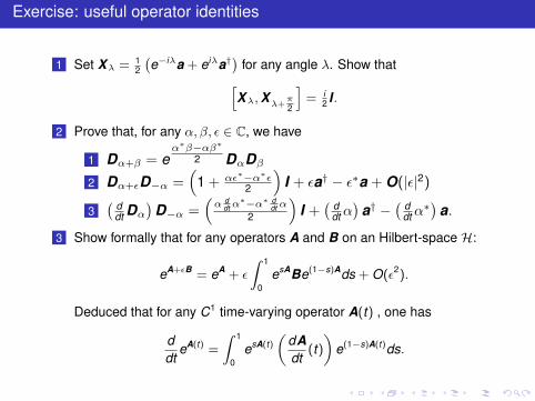
Exercise: useful operator identities
1 Set Xλ = 12
(e−iλa + eiλa†
)for any angle λ. Show that[
Xλ,Xλ+π2
]= i
2 I .
2 Prove that, for any α, β, ε ∈ C, we have
1 Dα+β = eα∗β−αβ∗
2 DαDβ
2 Dα+εD−α =(
1 + αε∗−α∗ε2
)I + εa† − ε∗a + O(|ε|2)
3( d
dt Dα
)D−α =
(α d
dt α∗−α∗ d
dt α
2
)I +
( ddtα)
a† −( d
dtα∗)a.
3 Show formally that for any operators A and B on an Hilbert-space H:
eA+εB = eA + ε
∫ 1
0esABe(1−s)Ads + O(ε2).
Deduced that for any C1 time-varying operator A(t) , one has
ddt
eA(t) =
∫ 1
0esA(t)
(dAdt
(t))
e(1−s)A(t)ds.

Quantum Control1
International Graduate School on Controlwww.eeci-igsc.eu
Pierre Rouchon2
Lecture 3Chengdu, July 8, 2019
1An important part of these slides gathered at the following web pagehave been elaborated with Mazyar Mirrahimi:http://cas.ensmp.fr/~rouchon/ChengduJuly2019/index.html
2Mines ParisTech, INRIA Paris
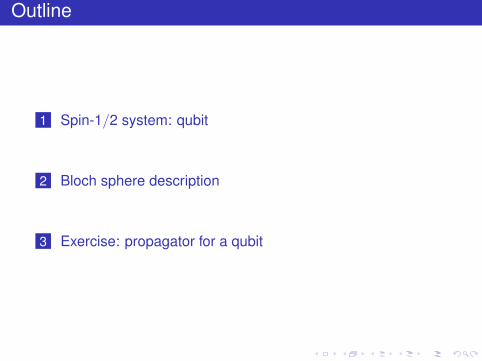
Outline
1 Spin-1/2 system: qubit
2 Bloch sphere description
3 Exercise: propagator for a qubit
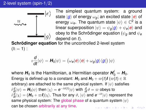
2-level system (spin-1/2)
The simplest quantum system: a groundstate |g〉 of energy ωg ; an excited state |e〉 ofenergy ωe. The quantum state |ψ〉 ∈ C2 is alinear superposition |ψ〉 = ψg |g〉+ ψe|e〉 andobey to the Schrödinger equation (ψg and ψedepend on t).
Schrödinger equation for the uncontrolled 2-level system(~ = 1) :
ıddt|ψ〉 = H0|ψ〉 =
(ωe|e〉〈e|+ ωg |g〉〈g|
)|ψ〉
where H0 is the Hamiltonian, a Hermitian operator H†0 = H0.Energy is defined up to a constant: H0 and H0 +$(t)I ($(t) ∈ Rarbitrary) are attached to the same physical system. If |ψ〉 satisfiesi d
dt |ψ〉 = H0|ψ〉 then |χ〉 = e−iϑ(t)|ψ〉 with ddt ϑ = $ obeys to
i ddt |χ〉 = (H0 +$I)|χ〉. Thus for any ϑ, |ψ〉 and e−iϑ|ψ〉 represent the
same physical system: The global phase of a quantum system |ψ〉can be chosen arbitrarily at any time.

The controlled 2-level system
Take origin of energy such that ωg (resp. ωe) becomes −ωe−ωg2
(resp. ωe−ωg2 ) and set ωeg = ωe − ωg
The solution of i ddt |ψ〉 = H0|ψ〉 =
ωeg2 (|e〉〈e| − |g〉〈g|)|ψ〉 is
|ψ〉t = ψg0eiωegt
2 |g〉+ ψe0e−iωegt
2 |e〉.With a classical electromagnetic field described by u(t) ∈ R,the coherent evolution the controlled Hamiltonian
H(t) =ωeg
2σz+
u(t)2
σx =ωeg
2(|e〉〈e|−|g〉〈g|)+
u(t)2
(|e〉〈g|+|g〉〈e|)
The controlled Schrödinger equation i ddt |ψ〉 = (H0 + u(t)H1)|ψ〉
reads:
iddt
(ψeψg
)=ωeg
2
(1 00 −1
)(ψeψg
)+
u(t)2
(0 11 0
)(ψeψg
).
The 3 Pauli Matrices3
σx = |e〉〈g|+ |g〉〈e|, σy = −i |e〉〈g|+ i |g〉〈e|, σz = |e〉〈e|−|g〉〈g|3They correspond, up to multiplication by i , to the 3 imaginary quaternions.

Pauli matrices and some formula
σx = |e〉〈g|+ |g〉〈e|, σy = −i |e〉〈g|+ i |g〉〈e|, σz = |e〉〈e| − |g〉〈g|σx
2 = I , σxσy = iσz , [σx ,σy ] = 2iσz , circular permutation . . .
Since for any θ ∈ R, eiθσx = cos θ + i sin θσx (idem for σyand σz ), the solution of i d
dt |ψ〉 =ωeg2 σz |ψ〉 is
|ψ〉t = e−iωegt
2 σz |ψ〉0 =
(cos
(ωegt
2
)I − i sin
(ωegt
2
)σz
)|ψ〉0
For α, β = x , y , z, α 6= β we have
σαeiθσβ = e−iθσβσα,(
eiθσα
)−1=(
eiθσα
)†= e−iθσα .
and also
e−iθ2 σασβe
iθ2 σα = e−iθσασβ = σβeiθσα

Density matrix and Bloch Sphere
We start from |ψ〉 that obeys i ddt |ψ〉 = H|ψ〉. We consider the
orthogonal projector on |ψ〉, ρ = |ψ〉〈ψ|, called density operator.Then ρ is an Hermitian operator ≥ 0, that satisfies Tr (ρ) = 1,ρ2 = ρ and obeys to the Liouville equation:
ddtρ = −i[H, ρ].
For a two level system |ψ〉 = ψg |g〉+ ψe|e〉 and
ρ =I + xσx + yσy + zσz
2where (x , y , z) = (2<(ψgψ
∗e),2=(ψgψ
∗e), |ψe|2 − |ψg |2) ∈ R3
represent a vector ~M = x~i + y~j + z~k , the Bloch vector, thatevolves on the unite sphere of R3, S2 called the the BlochSphere since Tr
(ρ2) = x2 + y2 + z2 = 1. The Liouville equation
with H =ωeg2 σz + u
2σx reads
ddt~M = (u~i + ωeg~k)× ~M.

Summary: 2-level system, i.e. a qubit (spin-half system)
Hilbert space:HM = C2 =
ψg |g〉+ ψe|e〉, ψg , ψe ∈ C
.
Quantum state space:D = ρ ∈ L(HM), ρ† = ρ,Tr (ρ) = 1, ρ ≥ 0 .Operators and commutations:σ- = |g〉〈e|, σ+ = σ-
† = |e〉〈g|σx = σ- + σ+ = |g〉〈e|+ |e〉〈g|;σy = iσ- − iσ+ = i |g〉〈e| − i |e〉〈g|;σz = σ+σ- − σ-σ+ = |e〉〈e| − |g〉〈g|;σx
2 = I , σxσy = iσz , [σx ,σy ] = 2iσz , . . .
Hamiltonian: HM = ωqσz/2 + uqσx .
Bloch sphere representation:D =
12
(I + xσx + yσy + zσz
) ∣∣ (x , y , z) ∈ R3, x2 + y2 + z2 ≤ 1
|g
|eωq
uq

Exercise: propagator for a qubit
Consider H = (uσx + vσy + wσz )/2 with (u, v ,w) ∈ R3.
1 For (u, v ,w) constant and non zero, compute the solutions of
ddt|ψ〉 = −iH|ψ〉, d
dtU = −iHU with U0 = I
in term of |ψ〉0, σ = (uσx + vσy + wσz )/√
u2 + v2 + w2 andω =√
u2 + v2 + w2. Indication: use the fact that σ2 = I .
2 Assume that, (u, v ,w) depends on t according to(u, v ,w)(t) = ω(t)(u, v , w) with (u, v , w) ∈ R3/0 constant oflength 1. Compute the solutions of
ddt|ψ〉 = −iH(t)|ψ〉, d
dtU = −iH(t)U with U0 = I
in term of |ψ〉0, σ = uσx + vσy + wσz and θ(t) =∫ t
0 ω.
3 Explain why (u, v ,w) colinear to the constant vector (u, v , w) iscrucial, for the computations in previous question.

Quantum Control1
International Graduate School on Controlwww.eeci-igsc.eu
Pierre Rouchon2
Lecture 4Chengdu, July 8, 2019
1An important part of these slides gathered at the following web pagehave been elaborated with Mazyar Mirrahimi:http://cas.ensmp.fr/~rouchon/ChengduJuly2019/index.html
2Mines ParisTech, INRIA Paris

Outline
1 Spin/spring systems
2 Exercise: the Jaynes-Cummings propagator
Outline
1 Spin/spring systems
2 Exercise: the Jaynes-Cummings propagator
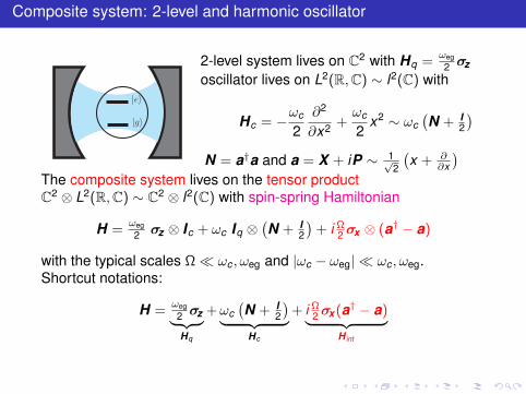
Composite system: 2-level and harmonic oscillator
|g〉
|e〉
1
2-level system lives on C2 with Hq =ωeg2 σz
oscillator lives on L2(R,C) ∼ l2(C) with
Hc = −ωc
2∂2
∂x2 +ωc
2x2 ∼ ωc
(N + I
2
)N = a†a and a = X + iP ∼ 1√
2
(x + ∂
∂x
)The composite system lives on the tensor productC2 ⊗ L2(R,C) ∼ C2 ⊗ l2(C) with spin-spring Hamiltonian
H =ωeg2 σz ⊗ Ic + ωc Iq ⊗
(N + I
2
)+ i Ω
2 σx ⊗ (a† − a)
with the typical scales Ω ωc , ωeg and |ωc − ωeg| ωc , ωeg.Shortcut notations:
H =ωeg2 σz︸ ︷︷ ︸Hq
+ωc(N + I
2
)︸ ︷︷ ︸Hc
+ i Ω2 σx (a† − a)︸ ︷︷ ︸
H int

The spin-spring PDE
The Schrödinger system
iddt|ψ〉 =
(ωeg2 σz + ωc
(N +
I2
)+ i Ω
2 σx (a† − a)
)|ψ〉
corresponds to two coupled scalar PDE’s:
i∂ψe
∂t= +
ωeg2 ψe + ωc
2
(x2 − ∂2
∂x2
)ψe − i
Ω√2∂
∂xψg
i∂ψg
∂t= −ωeg
2 ψg + ωc2
(x2 − ∂2
∂x2
)ψg − i
Ω√2∂
∂xψe
since N = a†a, a = 1√2
(x + ∂
∂x
)and |ψ〉 = (ψe(x , t), ψg(x , t)),
ψg(., t), ψe(., t) ∈ L2(R,C) and ‖ψg‖2 + ‖ψe‖2 = 1.
Exercise: write the PDE for the controlled Hamiltonianωeg2 σz + ωc
(N + I
2
)+ i Ω
2 σx (a† − a) + uc(a + a†) + uqσxwhere uc ,uq ∈ R are local control inputs associated to the oscillatorand qubit, respectively.

The spin-spring ODE’s
The Schrödinger system
iddt|ψ〉 =
(ωeg2 σz + ωc
(N + I
2
)+ i Ω
2 σx (a† − a))|ψ〉
corresponds also to an infinite set of ODE’s
iddtψe,n = ((n + 1/2)ωc + ωeg/2)ψe,n + i Ω
2
(√nψg,n−1 −
√n + 1ψg,n+1
)i
ddtψg,n = ((n + 1/2)ωc − ωeg/2)ψg,n + i Ω
2
(√nψe,n−1 −
√n + 1ψe,n+1
)where |ψ〉 =
∑+∞n=0 ψg,n|g,n〉+ ψe,n|e,n〉, ψg,n, ψe,n ∈ C.
Exercise: write the infinite set of ODE’s forωeg2 σz + ωc
(N + I
2
)+ i Ω
2 σx (a† − a) + uc(a + a†) + uqσxwhere uc ,uq ∈ R are local control inputs associated to the oscillatorand qubit, respectively.

Dispersive case: approximate Hamiltonian for Ω |ωc − ωeg|.
H ≈ Hdisp =ωeg2 σz + ωc
(N + I
2
)− χ
2σz(N + I
2
)with χ = Ω2
2(ωc−ωeg)
The corresponding PDE is :
i∂ψe
∂t= +
ωeg
2ψe +
12
(ωc −χ
2)(x2 − ∂2
∂x2 )ψe
i∂ψg
∂t= −ωeg
2ψg +
12
(ωc +χ
2)(x2 − ∂2
∂x2 )ψg
The propagator, the t-dependant unitary operator U solution ofi d
dt U = HU with U(0) = I , reads:
U(t) = eiωegt/2 exp(−i(ωc + χ/2)t(N + I
2 ))⊗ |g〉〈g|
+ e−iωegt/2 exp(−i(ωc − χ/2)t(N + I
2 ))⊗ |e〉〈e|
Exercise: write the infinite set of ODE’s attached to the dispersiveHamiltonian Hdisp.

Resonant case: approximate Hamiltonian for ωc = ωeg = ω.
The Hamiltonian becomes (Jaynes-Cummings Hamiltonian):
H ≈ HJC = ω2 σz + ω
(N +
I2
)+ i Ω
2 (σ-a† − σ+a).
The corresponding PDE is :
i∂ψe
∂t= +
ω
2ψe +
ω
2(x2 − ∂2
∂x2 )ψe − i Ω2√
2
(x +
∂
∂x
)ψg
i∂ψg
∂t= −ω
2ψg +
ω
2(x2 − ∂2
∂x2 )ψg + i Ω2√
2
(x − ∂
∂x
)ψe
Exercise: Write the infinite set of ODE’s attached to theJaynes-Cummings Hamiltonian H.

Exercise: the Jaynes-Cummings propagator
For HJC = ω2 σz + ω
(N + I
2
)+ i Ω
2 (σ-a† − σ+a) show that thepropagator, the t-dependant unitary operator U solution ofi d
dt U = HJCU with U(0) = I , reads
U(t) = e−iωt
(σz2 +N+
12
)e
Ωt2 (σ-a†−σ+a) where for any angle θ,
eθ(σ-a†−σ+a) = |g〉〈g| ⊗ cos(θ√
N) + |e〉〈e| ⊗ cos(θ√
N + I)
− σ+ ⊗ asin(θ
√N)√
N+ σ- ⊗
sin(θ√
N)√N
a†
Hint: show that[σz2 + N , σ-a† − σ+a
]= 0(
σ-a† − σ+a)2k
= (−1)k(|g〉〈g| ⊗ Nk + |e〉〈e| ⊗ (N + I)k
)(σ-a† − σ+a
)2k+1= (−1)k
(σ- ⊗ Nk a† − σ+ ⊗ aNk
)and compute de series defining the exponential of an operator.

Quantum Control1
International Graduate School on Controlwww.eeci-igsc.eu
Pierre Rouchon2
Lecture 5Chengdu, July 9, 2019
1An important part of these slides gathered at the following web pagehave been elaborated with Mazyar Mirrahimi:http://cas.ensmp.fr/~rouchon/ChengduJuly2019/index.html
2Mines ParisTech, INRIA Paris

Outline
1 Averaging and quasi-periodic control
2 First and second order averaging recipes
3 Exercise: resonant control of a qubit
Outline
1 Averaging and quasi-periodic control
2 First and second order averaging recipes
3 Exercise: resonant control of a qubit
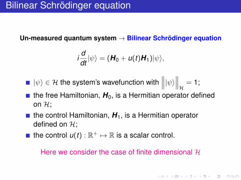
Bilinear Schrödinger equation
Un-measured quantum system→ Bilinear Schrödinger equation
iddt|ψ〉 = (H0 + u(t)H1)|ψ〉,
|ψ〉 ∈ H the system’s wavefunction with∥∥∥|ψ〉∥∥∥
H= 1;
the free Hamiltonian, H0, is a Hermitian operator definedon H;the control Hamiltonian, H1, is a Hermitian operatordefined on H;the control u(t) : R+ 7→ R is a scalar control.
Here we consider the case of finite dimensional H

Almost periodic control
We consider the controls of the form
u(t) = ε
r∑j=1
ujeiωj t + u∗j e−iωj t
ε > 0 is a small parameter;εuj is the constant complex amplitude associated to thepulsation ωj ≥ 0;r stands for the number of independent frequencies(ωj 6= ωk for j 6= k ).
We are interested in approximations, for ε tending to 0+, oftrajectories t 7→ |ψε〉t of
ddt|ψε〉 =
A0 + ε
r∑j=1
ujeiωj t + u∗j e−iωj t
A1
|ψε〉where A0 = −iH0 and A1 = −iH1 are skew-Hermitian.

Rotating frame
Consider the following change of variables
|ψε〉t = eA0t |φε〉t .
The resulting system is said to be in the “interaction frame”ddt|φε〉 = εB(t)|φε〉
where B(t) is a skew-Hermitian operator whosetime-dependence is almost periodic:
B(t) =r∑
j=1
ujeiωj te−A0tA1eA0t + u∗j e−iωj te−A0tA1eA0t .
Main idea
We can writeB(t) = B +
ddt
B(t),
where B is a constant skew-Hermitian matrix and B(t) is abounded almost periodic skew-Hermitian matrix.

Multi-frequency averaging: first order
Consider the two systemsddt|φε〉 = ε
(B +
ddt
B(t))|φε〉,
andddt|φ1stε 〉 = εB|φ1st
ε 〉,
initialized at the same state |φ1stε 〉0 = |φε〉0.
Theorem: first order approximation (Rotating WaveApproximation)
Consider the functions |φε〉 and |φ1stε 〉 initialized at the same
state and following the above dynamics. Then, there existM > 0 and η > 0 such that for all ε ∈]0, η[ we have
maxt∈[
0,1ε
]∥∥∥|φε〉t − |φ1stε 〉t
∥∥∥ ≤ Mε

Multi-frequency averaging: first order
Proof’s idea
Almost periodic change of variables:
|χε〉 = (1− εB(t))|φε〉
well-defined for ε > 0 sufficiently small.The dynamics can be written as
ddt|χε〉 = (εB + ε2F (ε, t))|χε〉
where F (ε, t) is uniformly bounded in time.

Multi-frequency averaging: second orderMore precisely, the dynamics of |χε〉 is given by
ddt|χε〉 =
(εB + ε2[B, B(t)]− ε2B(t)
ddt
B(t) + ε3E(ε, t))|χε〉
E(ε, t) is still almost periodic but its entries are no more linearcombinations of time-exponentials;
B(t) ddt B(t) is an almost periodic operator whose entries are
linear combinations of oscillating time-exponentials.
We can write
B(t) =ddt
C(t) and B(t)ddt
B(t) = D +ddt
D(t)
where C(t) and D(t) are almost periodic. We have
ddt|χε〉 =
(εB − ε2D + ε2
ddt
([B, C(t)]− D(t)
)+ ε3E(ε, t)
)|χε〉
where the skew-Hermitian operators B and D are constants and theother ones C, D, and E are almost periodic.
Multi-frequency averaging: second order
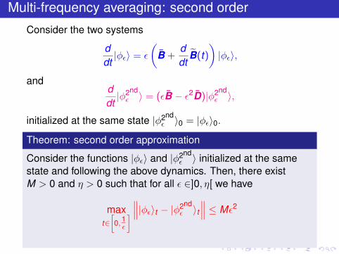
Consider the two systems
ddt|φε〉 = ε
(B +
ddt
B(t))|φε〉,
andddt|φ2ndε 〉 = (εB − ε2D)|φ2nd
ε 〉,
initialized at the same state |φ2ndε 〉0 = |φε〉0.
Theorem: second order approximation
Consider the functions |φε〉 and |φ2ndε 〉 initialized at the same
state and following the above dynamics. Then, there existM > 0 and η > 0 such that for all ε ∈]0, η[ we have
maxt∈[
0,1ε
]∥∥∥|φε〉t − |φ2ndε 〉t
∥∥∥ ≤ Mε2

Multi-frequency averaging: second order
Proof’s idea
Another almost periodic change of variables
|ξε〉 =(
I − ε2(
[B, C(t)]− D(t)))|χε〉.
The dynamics can be written as
ddt|ξε〉 =
(εB − ε2D + ε3F (ε, t)
)|ξε〉
where εB − ε2D is skew Hermitian and F is almost periodic andtherefore uniformly bounded in time.

Outline
1 Averaging and quasi-periodic control
2 First and second order averaging recipes
3 Exercise: resonant control of a qubit

The Rotating Wave Approximation (RWA) recipes
Schrödinger dynamics i ddt |ψ〉 = H(t)|ψ〉, with
H(t) = H0 +m∑
k=1
uk (t)Hk , uk (t) =r∑
j=1
uk,jeiωj t + u∗k,je−iωj t .
The Hamiltonian in interaction frame
H int(t) =∑k,j
(uk,jeiωj t + u∗k,je
−iωj t)
eiH0tHk e−iH0t
We define the first order Hamiltonian
H1strwa = H int = lim
T→∞
1T
∫ T
0H int(t)dt ,
and the second order Hamiltonian
H2ndrwa = H1st
rwa − i(H int − H int
)(∫t(H int − H int)
)Choose the amplitudes uk,j and the frequencies ωj such that the
propagators of H1strwa or H2nd
rwa admit simple explicit forms that are usedto find t 7→ u(t) steering |ψ〉 from one location to another one.

Exercise: resonant control of a qubit
In i ddt |ψ〉 =
(ωeg2 σz + u
2σx)|ψ〉, take a resonant control u(t) = ueiωegt + u∗e−iωeg t
with u slowly varying complex amplitude∣∣∣ d
dt u∣∣∣ ωeg|u|. Set H0 =
ωeg2 σz and
εH1 = u2σx
1 Consider |ψ〉 = e−iωeg t
2 σz |φ〉 and show that i ddt |φ〉 = H int|φ〉 with
H int = u(t)2 eiωegt
σ+=|e〉〈g|︷ ︸︸ ︷σx + iσy
2+ u(t)
2 e−iωegt
σ-=|g〉〈e|︷ ︸︸ ︷σx − iσy
2.
2 Show that up to second order terms one has i ddt |φ〉 = H1st
rwa|φ〉 with
H1strwa = u∗σ++uσ-
2 .3 Take constant control u = Ωr eiθ for t ∈ [0,T ], T > 0. Show that |φ〉 is solution
of (Σ) : i ddt |φ〉 =
Ωr (cos θσx +sin θσy )2 |φ〉.
4 Set Θr = Ωr2 T . Show that the solution at T of the propagator U t ∈ SU(2),
i ddt U =
Ωr (cos θσx +sin θσy )2 U, U0 = I is given by
UT = cos Θr I − i sin Θr (cos θσx + sin θσy ) ,
5 Take a wave function |φ〉. Show that exist Ωr and θ such that UT |g〉 = eiα|φ〉,where α is some global phase.
6 Prove that for any given two wave functions |φa〉 and |φb〉 exists a piece-wiseconstant control [0, 2T ] 3 t 7→ u(t) ∈ C such that the solution of (Σ) with|φ〉0 = |φa〉 satisfies |φ〉T = eiβ |φb〉 for some global phase β.

Quantum Control1
International Graduate School on Controlwww.eeci-igsc.eu
Pierre Rouchon2
Lecture 6Chengdu, July 9, 2019
1An important part of these slides gathered at the following web pagehave been elaborated with Mazyar Mirrahimi:http://cas.ensmp.fr/~rouchon/ChengduJuly2019/index.html
2Mines ParisTech, INRIA Paris

The Rotating Wave Approximation (RWA) recipes
Schrödinger dynamics i ddt |ψ〉 = H(t)|ψ〉, with
H(t) = H0 +m∑
k=1
uk (t)Hk , uk (t) =r∑
j=1
uk,jeiωj t + u∗k,je−iωj t .
The Hamiltonian in interaction frame
H int(t) =∑k,j
(uk,jeiωj t + u∗k,je
−iωj t)
eiH0tHk e−iH0t
We define the first order Hamiltonian
H1strwa = H int = lim
T→∞
1T
∫ T
0H int(t)dt ,
and the second order Hamiltonian
H2ndrwa = H1st
rwa − i(H int − H int
)(∫t(H int − H int)
)Choose the amplitudes uk,j and the frequencies ωj such that the
propagators of H1strwa or H2nd
rwa admit simple explicit forms that are usedto find t 7→ u(t) steering |ψ〉 from one location to another one.

Outline
1 Averaging of spin/spring systemsThe spin/spring modelResonant interaction (Jaynes-Cummings system)Dispersive interaction
2 Exercise: control of the Jaynes-Cummings system
Outline
1 Averaging of spin/spring systemsThe spin/spring modelResonant interaction (Jaynes-Cummings system)Dispersive interaction
2 Exercise: control of the Jaynes-Cummings system

The spin/spring model
The Schrödinger system
iddt|ψ〉 =
(ωeg2 σz + ωc
(a†a +
I2
)+ i Ω
2 σx (a† − a)
)|ψ〉
corresponds to two coupled scalar PDE’s:
i∂ψe
∂t= +
ωeg
2ψe +
ωc
2
(x2 − ∂2
∂x2
)ψe − i
Ω√2∂
∂xψg
i∂ψg
∂t= −
ωeg
2ψg +
ωc
2
(x2 − ∂2
∂x2
)ψg − i
Ω√2∂
∂xψe
since a = 1√2
(x + ∂
∂x
)and |ψ〉 corresponds to (ψe(x , t), ψg(x , t))
where ψe(., t), ψg(., t) ∈ L2(R,C) and ‖ψe‖2 + ‖ψg‖2 = 1.

Resonant case: passage to the interaction frame
In H~ =
ωeg2 σz + ωc
(a†a + I
2
)+ i Ω
2 σx (a† − a), ωeg = ωc = ω with|Ω| ω. Then H = H0 + εH1 where ε is a small parameter and
H0
~= ω
2 σz + ω
(a†a +
I2
)εH1
~= i Ω
2 σx (a† − a).
H int is obtained by setting |ψ〉 = e−iωt(a†a+ I2 )e
−iωt2 σz |φ〉 in
i~ ddt |ψ〉 = H|ψ〉 to get i~ d
dt |φ〉 = H int|φ〉 with
H int~
= i Ω2
(e−iωtσ- + eiωtσ+
)(eiωta† − e−iωta
)where we used
eiθ2 σz σxe−
iθ2 σz = e−iθσ- + eiθσ+, eiθ(a†a+ I
2 ) a e−iθ(a†a+ I2 ) = e−iθa

Resonant spin/spring Hamiltonian and associated PDE
The secular terms in H int are given by (RWA, first order
approximation) H1strwa/~ = i Ω
2
(σ-a† − σ+a
). Since quantum state
|φ〉 = e+iωt(a†a+ I2 )e
+iωt2 σz |ψ〉 obeys approximatively to
i~ ddt |φ〉 = H1st
rwa|φ〉, the original quantum state |ψ〉 is governed by
iddt|ψ〉 =
(ω2 σz + ω
(a†a +
I2
)+ i Ω
2
(σ-a† − σ+a
))|ψ〉
The Jaynes-Cummings Hamiltonian (ωeg = ωc = ω) reads:
HJC/~ = ω2 σz + ω
(a†a +
I2
)+ i Ω
2
(σ-a† − σ+a
)The corresponding PDE is :
i∂ψe
∂t= +
ω
2ψe +
ω
2(x2 − ∂2
∂x2 )ψe − i Ω2√
2
(x − ∂
∂x
)ψg
i∂ψg
∂t= −ω
2ψg +
ω
2(x2 − ∂2
∂x2 )ψg + i Ω2√
2
(x +
∂
∂x
)ψe
Dispersive case: passage to the interaction frame
H~ =
ωeg2 σz + ωc
(a†a + I
2
)+ i Ω
2 σx (a† − a)with |Ω| |ωeg − ωc | ωeg, ωc .Then H = H0 + εH1 where ε is a small parameter and
H0~ =
ωeg2 σz + ωc
(a†a + I
2
), εH1
~ = i Ω2 σx (a† − a).
H int is obtained by setting |ψ〉 = e−iωc t(a†a+ I2 )e
−iωeg t2 σz |φ〉 in
i~ ddt |ψ〉 = H|ψ〉 to get i~ d
dt |φ〉 = H int|φ〉 with
H int~
= i Ω2
(e−iωegtσ- + eiωegtσ+
)(eiωc ta† − e−iωc ta
)= i Ω
2
(ei(ωc−ωeg)tσ-a† − e−i(ωc−ωeg)tσ+a + ei(ωc+ωeg)tσ+a† − e−i(ωc+ωeg)tσ-a
)Thus H1st
rwa = H int = 0: no secular term. We have to compute
H2ndrwa = H int − i
(H int − H int
) (∫t (H int − H int)
)where
∫t (H int − H int/~
corresponds to
Ω2
(ei(ωc−ωeg)t
ωc−ωegσ-a† + e−i(ωc−ωeg)t
ωc−ωegσ+a + ei(ωc +ωeg)t
ωc+ωegσ+a† + e−i(ωc +ωeg)t
ωc+ωegσ-a)

Dispersive spin/spring Hamiltonian and associated PDE
The secular terms in H2ndrwa are
Ω2
4(ωc−ωeg)
(σ-σ+a†a − σ+σ-aa†
)+ Ω2
4(ωc+ωeg)
(− σ-σ+aa† + σ+σ-a†a
)Since |Ω| |ωeg − ωc | ωeg, ωc , we have Ω2
4(ωc+ωeg) Ω2
4(ωc−ωeg)
H2ndrwa/~ ≈ − Ω2
4(ωc−ωeg)
(σz(N + I
2
)+ I
2
).
Since quantum state |φ〉 = e+iωc t(N+ I2 )e
+iωeg t2 σz |ψ〉 obeys
approximatively to i~ ddt |φ〉 = H2nd
rwa |φ〉, the original quantum state |ψ〉 is
governed by i ddt |ψ〉 =
(Hdisp~ −
Ω2
8(ωc−ωeg)
)|ψ〉 with
Hdisp/~ =ωeg2 σz + ωc
(N + I
2
)− χ
2σz(N + I
2
)and χ = Ω2
2(ωc−ωeg)
The corresponding PDE is :
i∂ψe
∂t= +
ωeg
2ψe +
12
(ωc −χ
2)(x2 − ∂2
∂x2 )ψe
i∂ψg
∂t= −
ωeg
2ψg +
12
(ωc +χ
2)(x2 − ∂2
∂x2 )ψg

Outline
1 Averaging of spin/spring systemsThe spin/spring modelResonant interaction (Jaynes-Cummings system)Dispersive interaction
2 Exercise: control of the Jaynes-Cummings system
Exercise: control of the Jaynes-Cummings system
Consider the spin-spring model with Ω |ω|:H~ = ω
2 σz + ω(
a†a + I2
)+ i Ω
2 σx (a† − a) + u(a + a†)with a real control input u(t) ∈ R:
1 Show that with the resonant control u(t) = ue−iωt + u∗e+iωt with complexamplitude u such that |u| ω, the first order RWA approximation yields to thefollowing dynamics in the interaction frame
i ddt |ψ〉 =
(i Ω
2 (σ-a† − σ+a) + ua† + u∗a)|ψ〉
2 Set v ∈ C solution of ddt v = −iu and consider the following change of frame
|φ〉 = D−v|ψ〉 with the displacement operator D−v = e−va†+v∗a. Show that, upto a global phase change, we have, with u = i Ω
2 v,
i ddt |φ〉 =
(iΩ2
(σ-a† − σ+a) + (uσ+ + u∗σ-)
)|φ〉
3 Take the orthonormal basis |g, n〉, |e, n〉 with n ∈ N being the photon numberand where for instance |g, n〉 stands for the tensor product |g〉 ⊗ |n〉. Set|φ〉 =
∑n φg,n|g, n〉+ φe,n|e, n〉 with φg,n, φe,n ∈ C depending on t and∑
n |φg,n|2 + |φe,n|2 = 1. Show that, for n ≥ 0i d
dt φg,n+1 = i Ω2
√n + 1φe,n + u∗φe,n+1, i d
dt φe,n = −i Ω2
√n + 1φg,n+1 + uφg,n
and i ddt φg,0 = u∗φe,0.
4 Assume that |φ〉0 = |g, 0〉. Construct an open-loop control [0,T ] 3 t 7→ u(t)such that |φ〉T ≈ |g, 1〉 (hint: use an impulse for t ∈ [0, ε] followed by 0 on [ε,T ]with ε T and well chosen T ).
5 Generalize the above open-loop control when the goal state |φ〉T is |g, n〉 withany arbitrary photon number n.
Quantum Control1
International Graduate School on Controlwww.eeci-igsc.eu
Pierre Rouchon2
Lecture 7Chengdu, July 10, 2019
1An important part of these slides gathered at the following web pagehave been elaborated with Mazyar Mirrahimi:http://cas.ensmp.fr/~rouchon/ChengduJuly2019/index.html
2Mines ParisTech, INRIA Paris

Outline
1 Discrete-time dynamics of the LKB photon boxGeneral structure based on three quantum featuresDispersive probe qubitsResonant probe qubitsDensity operator to cope with measurement imperfections
2 Exercise: Markov process including detection errors

Three quantum features emphasized by the LKB photon box 3
1 Schrödinger (~ = 1): wave function |ψ〉 in Hilbert space H,
ddt|ψ〉 = −iH|ψ〉, H = H0 + uH1.
Unitary propagator U solution of ddt U = −iHU with U(0) = I.
2 Origin of dissipation: collapse of the wave packet induced by themeasurement of observable O with spectral decomp.
∑µ λµPµ:
measurement outcome µ with proba. Pµ = 〈ψ|Pµ|ψ〉 dependingon |ψ〉, just before the measurementmeasurement back-action if outcome µ = y :
|ψ〉 7→ |ψ〉+ =Py |ψ〉√〈ψ|Py |ψ〉
3 Tensor product for the description of composite systems (S,M):Hilbert space H = HS ⊗HM
Hamiltonian H = HS ⊗ IM + H int + IS ⊗ HM
observable on sub-system M only: O = IS ⊗OM .
3S. Haroche and J.M. Raimond. Exploring the Quantum: Atoms, Cavitiesand Photons. Oxford Graduate Texts, 2006.

Composite system built with a harmonic oscillator and a qubit.
System S corresponds to a quantized harmonic oscillator:
HS = Hc =
∞∑n=0
cn|n〉∣∣∣∣ (cn)∞n=0 ∈ l2(C)
,
where |n〉 represents the Fock state associated to exactly nphotons inside the cavityMeter M is a qubit, a 2-level system: HM = Ha = C2, eachatom admits two energy levels and is described by a wavefunction cg |g〉+ ce|e〉 with |cg |2 + |ce|2 = 1;State of the full system |Ψ〉 ∈ HS ⊗HM = Hc ⊗Ha:
|Ψ〉 =+∞∑n=0
cng |n〉 ⊗ |g〉+ cne|n〉 ⊗ |e〉, cne, cng ∈ C.
Ortho-normal basis: (|n〉 ⊗ |g〉, |n〉 ⊗ |e〉)n∈N.

Markov model (1)
C
B
D
R 1R 2
B R 2
When atom comes out B, |Ψ〉B of the full system is separable|Ψ〉B = |ψ〉 ⊗ |g〉.
Just before the measurement in D, the state is in generalentangled (not separable):
|Ψ〉R2 = USM(|ψ〉 ⊗ |g〉
)=(Mg |ψ〉
)⊗ |g〉+
(Me|ψ〉
)⊗ |e〉
where USM is a unitary transformation (Schrödinger propagator)defining the linear measurement operators Mg and Me on HS.Since USM is unitary, M†gMg + M†eMe = I .

Markov model (2)
Just before D, the field/atom state is entangled:
Mg |ψ〉 ⊗ |g〉+ Me|ψ〉 ⊗ |e〉
Denote by µ ∈ g,e the measurement outcome in detector D: withprobability Pµ =
⟨ψ|M†µMµ|ψ
⟩we get µ. Just after the measurement
outcome µ = y , the state becomes separable:
|Ψ〉D = 1√Py
(My |ψ〉)⊗ |y〉 =
(My√
〈ψ|M†y My |ψ〉|ψ〉
)⊗ |y〉.
Markov process: |ψk 〉 ≡ |ψ〉t=k∆t , k ∈ N, ∆t sampling period,
|ψk+1〉 =
Mg |ψk 〉√〈ψk |M†g Mg |ψk〉
with yk = g, probability Pg =⟨ψk |M†gMg |ψk
⟩;
Me|ψk 〉√〈ψk |M†e Me|ψk〉
with yk = e, probability Pe =⟨ψk |M†eMe|ψk
⟩.

Dispersive case
UR1 =
(|g〉+ |e〉√
2
)〈g|+
(|g〉 − |e〉√
2
)〈e|
UR2 =
(|g〉+ e−iφR |e〉√
2
)〈g|+
(eiφR |g〉 − |e〉√
2
)〈e|
UC = e−iφ02 N |g〉〈g|+ ei
φ02 N |e〉〈e|
where φ0 and φR are constant parameters.The measurement operators Mg and Me are the followingbounded operators:
Mg = cos(φR+φ0N
2
), Me = sin
(φR+φ0N
2
)up to irrelevant global phases.Exercise: prove the above formulae for Mg and Me.
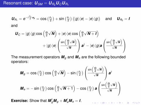
Resonant case: USM = UR2UCUR1
UR1 = e−i θ12 σy = cos
(θ12
)+ sin
(θ12
) (|g〉〈e| − |e〉〈g|
)and UR2 = I
and
UC = |g〉〈g| cos(
Θ2
√N)
+ |e〉〈e| cos(
Θ2
√N + I
)+ |g〉〈e|
sin(
Θ2√
N)
√N
a† − |e〉〈g|a
sin(
Θ2√
N)
√N
The measurement operators Mg and Me are the following boundedoperators:
Mg = cos(θ12
)cos
(Θ2
√N)− sin
(θ12
) sin(
Θ2√
N)
√N
a†
Me = − sin(θ12
)cos
(Θ2
√N + 1
)− cos
(θ12
)a
sin(
Θ2√
N)
√N
Exercise: Show that M†gMg + M†eMe = I .

Markov process with detection inefficiency
With pure state ρ = |ψ〉〈ψ|, we have
ρ+ = |ψ+〉〈ψ+| =1
Tr(
MµρM†µ)MµρM†µ
when the atom collapses in µ = g,e with proba. Tr(
MµρM†µ)
.
Detection efficiency: the probability to detect the atom isη ∈ [0,1]. Three possible outcomes for y : y = g if detection in g,y = e if detection in e and y = 0 if no detection.
The only possible update is based on ρ: expectation ρ+ of |ψ+〉〈ψ+|knowing ρ and the outcome y ∈ g,e,0.
ρ+ =
MgρM†g
Tr(MgρMg) if y = g, probability η Tr (MgρMg)
MeρM†eTr(MeρMe) if y = e, probability η Tr (MeρMe)
MgρM†g + MeρM†e if y = 0, probability 1− η
For η = 0: ρ+ = MgρM†g + MeρM†e = K(ρ) = E(ρ+ | ρ
)defines a
Kraus map.

Several operator spaces
H separable Hilbert space. Pure states |ψ〉 are unitary vectors ofH also called (probability amplitude) wave functions.
L(H) is the space of linear operators from H to H: it containsthe spaces of
bounded operators (Banach space B(H) with sup-norm)compact operators (space Kc(H))Hilbert-Schmidt operators (Hilbert space K2(H) with theFrobenius norm)trace class operators (Banach space K1(H) with the tracenorm).
the most general quantum state ρ is non negative Hermitiantrace class operator of trace one. ρ live in a closed convexsubset of K1(H).If Tr
(ρ2)
= 1 then ρ = |ψ〉〈ψ| where |ψ〉 is pure state.
For H of finite dimension, these operator spaces coincide. For H ofinfinite dimension, they are all different:
dimH =∞ ⇒ K1(H) $ K2(H) $ Kc(H) $ B(H) $ L(H).

LKB photon-box: Markov process with detection errors (1)
With pure state ρ = |ψ〉〈ψ|, we have
ρ+ = |ψ+〉〈ψ+| =1
Tr(
MµρM†µ)MµρM†µ
when the atom collapses in µ = g,e with proba. Tr(
MµρM†µ)
.
Detection error rates: P(y = e/µ = g) = ηg ∈ [0,1] theprobability of erroneous assignation to e when the atomcollapses in g; P(y = g/µ = e) = ηe ∈ [0,1] (given by thecontrast of the Ramsey fringes).
Bayesian law: expectation ρ+ of |ψ+〉〈ψ+| knowing ρ and theimperfect detection y .
ρ+ =
(1−ηg)MgρM†g +ηeMeρM†e
Tr((1−ηg)MgρM†g +ηeMeρM†e )if y = g, prob. Tr
((1− ηg)MgρM†g + ηeMeρM†e
);
ηgMgρM†g +(1−ηe)MeρM†eTr(ηgMgρM†g +(1−ηe)MeρM†e )
if y = e, prob. Tr(ηgMgρM†g + (1− ηe)MeρM†e
).
ρ+ does not remain pure: the quantum state ρ+ becomes a mixedstate; |ψ+〉 becomes physically irrelevant.

LKB photon-box: Markov process with detection errors (2)
We get
ρ+ =
(1−ηg)MgρM†g +ηeMeρM†e
Tr((1−ηg)MgρM†g +ηeMeρM†e ), with prob. Tr
((1− ηg)MgρM†g + ηeMeρM†e
);
ηgMgρM†g +(1−ηe)MeρM†eTr(ηgMgρM†g +(1−ηe)MeρM†e )
with prob. Tr(ηgMgρM†g + (1− ηe)MeρM†e
).
Key point:
Tr(
(1− ηg)MgρM†g + ηeMeρM†e)
and Tr(ηgMgρM†g + (1− ηe)MeρM†e
)are the probabilities to detect y = g and e, knowing ρ.Reformulation with quantum maps : set
Kg(ρ) = (1−ηg)MgρM†g+ηeMeρM†e, Ke(ρ) = ηgMgρM†g+(1−ηe)MeρM†e.
ρ+ =Ky (ρ)
Tr (Ky (ρ))when we detect y
The probability to detect y knowing ρ is Tr (Ky (ρ)).We have the following Kraus map:
E(ρ+ | ρ
)= Kg(ρ) + Ke(ρ) = K(ρ) = MgρM†g + MeρM†e.

Exercise: Markov process including detection errors
Consider a set of N bounded operators Mµ on an Hilbert spaceH such that∑µ M†µMµ = I . Take the ideal
Markov process ρk+1 =Mµρk M†µ
Tr(
Mµρk M†µ) and ideal measurement outcomes µ ∈ 1, . . . ,N of probability
Tr(
Mµρk M†µ)
. Assume that the real measurement process provides Nd different values y ∈ 1, . . . ,Ndcorrelated to the ideal measurement µ via the following conditional classical probabilities P (y | µ) = ηy,µ ∈ [0, 1]where η is a left stochastic matrix (
∑y ηy,µ = 1 for each µ).
Denote by ρk the expectation value of ρk knowing ρ0 and the real measurement outcomes y0, . . . , yk−1 at steps0, . . . , k − 1. Consider the un-normalized ideal quantum state
ξµ0,...,µk= Mµk . . .Mµ0ρ0M†µ0
. . .M†µk
associated to the ideal outcomes µ0, . . . , µk .
1 Show that P (µ0, . . . , µk | ρ0) = Tr(ξµ0,...,µk
).
2 Using Bayes law, prove that
P (y0, . . . , yk | ρ0) =N∑
µk =1
. . .N∑
µ0=1
ηy0,µ0 . . . ηyk ,µk Tr(ξµ0,...,µk
).
3 Using Bayes law, prove also that
P (µ0, . . . , µk | y0, . . . , yk , ρ0) =ηy0,µ0 . . . ηyk ,µk Tr
(ξµ0,...,µk
)P (y0, . . . , yk | ρ0)
4 Prove for ` = 1, . . . , k − 1 that ρ`+1 =
∑Nµ=1 ηy`,µMµρ`M†µ
Tr(∑N
µ=1 ηy`,µMµρ`M†µ) and that
P(y` | y0, . . . , y`−1,ρ0
)= Tr
(∑Nµ=1 ηy`,µM†µρ`Mµ
)(hint: use the un-normalized estimate
ξy0,...,y`colinear to ρ`+1).

Quantum Control1
International Graduate School on Controlwww.eeci-igsc.eu
Pierre Rouchon2
Lecture 8Chengdu, July 10, 2019
1An important part of these slides gathered at the following web pagehave been elaborated with Mazyar Mirrahimi:http://cas.ensmp.fr/~rouchon/ChengduJuly2019/index.html
2Mines ParisTech, INRIA Paris

Outline
1 Quantum measurement and filteringProjective measurementPositive Operator Valued Measurement (POVM)Stochastic process attached to POVMQuantum Filtering
2 Convergence issues with Schrödinger and Heisenbergpictures
3 Exercise: cooling with resonant qubits in |g〉

Outline
1 Quantum measurement and filteringProjective measurementPositive Operator Valued Measurement (POVM)Stochastic process attached to POVMQuantum Filtering
2 Convergence issues with Schrödinger and Heisenbergpictures
3 Exercise: cooling with resonant qubits in |g〉

Projective measurement
For the system defined on Hilbert space H, take
an observable O (Hermitian operator) defined on H:
O =∑ν
λνPν ,
where λν ’s are the eigenvalues of O and Pν is the projectionoperator over the associated eigenspace.
a quantum state given by the wave function |ψ〉 in H.
Projective measurement of the physical observable O =∑ν λνPν for
the quantum state |ψ〉:1 The probability of obtaining the value λν is given by
Pν = 〈ψ|Pν |ψ〉; note that∑ν Pν = 1 as
∑ν Pν = IH (IH
represents the identity operator of H).
2 After the measurement, the conditional (a posteriori) state |ψ+〉of the system, given the outcome λν , is
|ψ+〉 =Pν |ψ〉√
Pν(collapse of the wave packet).

Positive Operator Valued Measurement (POVM) (1)
System S of interest (a quantized electromagnetic field) interacts withthe meter M (a probe atom), and the experimenter measuresprojectively the meter M (the probe atom). Need for a Compositesystem: HS ⊗HM where HS and HM are Hilbert spaces of S and M.Measurement process in three successive steps:
1 Initially the quantum state is separable
HS ⊗HM 3 |Ψ〉 = |ψS〉 ⊗ |ψM〉
with a well defined and known state |ψM〉 for M.
2 Then a Schrödinger evolution during a small time (unitaryoperator US,M ) of the composite system from |ψS〉 ⊗ |ψM〉 andproducing US,M
(|ψS〉 ⊗ |ψM〉
), entangled in general.
3 Finally a projective measurement of the meter M:OM = IS ⊗
(∑ν λνPν
)the measured observable for the meter.
Projection operator Pν is a rank-1 projection in HM over theeigenstate |ξν〉 ∈ HM : Pν = |ξν〉〈ξν |.

Positive Operator Valued Measurement (POVM) (2)
Define the measurement operators Mν via
∀|ψS〉 ∈ HS, US,M(|ψS〉 ⊗ |ψM〉
)=∑ν
(Mν |ψS〉
)⊗ |ξν〉.
Then∑
ν M†νMν = IS. The set Mν defines a PositiveOperator Valued Measurement (POVM).In HS ⊗HM , projective measurement of OM = IS ⊗
(∑ν λνPν
)with quantum state US,M
(|ψS〉 ⊗ |ψM〉
):
1 The probability of obtaining the value λν is given byPν = 〈ψS|M†νMν |ψS〉
2 After the measurement, the conditional (a posteriori) stateof the system, given the outcome ν, is
|ψS,+〉 =Mν |ψS〉√
Pν.

Stochastic processes attached to a POVM
To the POVM (Mν) on HS is attached a stochastic process of quantumstate |ψ〉
|ψ+〉 =Mν |ψ〉√
Pνwith probability Pν = 〈ψ|M†νMν |ψ〉
For any observable A on HS , its conditional expectation value after thetransition knowing the state |ψ〉
E(〈ψ+|A|ψ+〉
∣∣∣ |ψ〉) = 〈ψ|(∑ν
M†νAMν)|ψ〉 = Tr (A K (|ψ〉〈ψ|))
with Kraus map K (ρ) =∑ν MνρM†ν with ρ = |ψ〉〈ψ| density operator
corresponding to |ψ〉.Imperfection and errors described by left stochastic matrix (ηy,ν) whereηy,ν is the probability of detector outcome y knowing that the idealdetection ν (
∑y ηy,ν ≡ 1). Then Bayes law yields
E(ρ+
∣∣ ρ, y) =K y (ρ)
Tr (K y (ρ))
with completely positive linear maps K y (ρ) =∑ν ηy,νMνρM†ν
depending on y . Probability to detect y knowing ρ is Tr (K y (ρ).
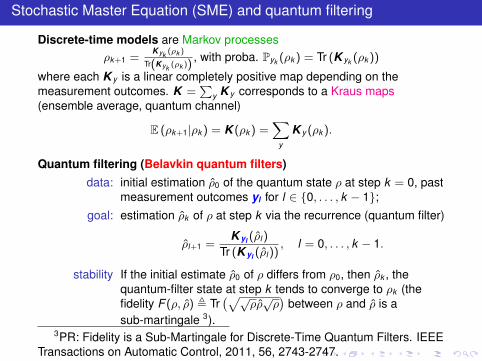
Stochastic Master Equation (SME) and quantum filtering
Discrete-time models are Markov processesρk+1 =
K yk (ρk )
Tr(K yk (ρk )), with proba. Pyk (ρk ) = Tr (K yk (ρk ))
where each K y is a linear completely positive map depending on themeasurement outcomes. K =
∑y K y corresponds to a Kraus maps
(ensemble average, quantum channel)
E (ρk+1|ρk ) = K (ρk ) =∑
y
K y (ρk ).
Quantum filtering (Belavkin quantum filters)data: initial estimation ρ0 of the quantum state ρ at step k = 0, past
measurement outcomes yl for l ∈ 0, . . . , k − 1;goal: estimation ρk of ρ at step k via the recurrence (quantum filter)
ρl+1 =K yl (ρl )
Tr (K yl (ρl )), l = 0, . . . , k − 1.
stability If the initial estimate ρ0 of ρ differs from ρ0, then ρk , thequantum-filter state at step k tends to converge to ρk (thefidelity F (ρ, ρ) , Tr
(√√ρρ√ρ)
between ρ and ρ is asub-martingale 3).
3PR: Fidelity is a Sub-Martingale for Discrete-Time Quantum Filters. IEEETransactions on Automatic Control, 2011, 56, 2743-2747.

Outline
1 Quantum measurement and filteringProjective measurementPositive Operator Valued Measurement (POVM)Stochastic process attached to POVMQuantum Filtering
2 Convergence issues with Schrödinger and Heisenbergpictures
3 Exercise: cooling with resonant qubits in |g〉
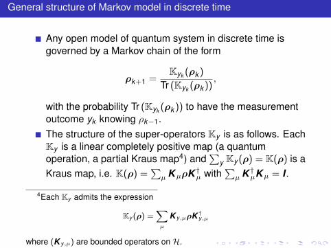
General structure of Markov model in discrete time
Any open model of quantum system in discrete time isgoverned by a Markov chain of the form
ρk+1 =Kyk (ρk )
Tr (Kyk (ρk )),
with the probability Tr (Kyk (ρk )) to have the measurementoutcome yk knowing ρk−1.The structure of the super-operators Ky is as follows. EachKy is a linear completely positive map (a quantumoperation, a partial Kraus map4) and
∑y Ky (ρ) = K(ρ) is a
Kraus map, i.e. K(ρ) =∑
µ KµρK †µ with∑
µ K †µKµ = I .
4Each Ky admits the expression
Ky (ρ) =∑µ
K y,µρK †y,µ
where (K y,µ) are bounded operators on H.

Schrödinger view point of ensemble average dynamics
Without measurement record, the quantum state ρk obeys to themaster equation
ρk+1 = K(ρk ).
since E (ρk+1 | ρk ) = K(ρk ) (ensemble average).
K is always a contraction (not strict in general ) for the followingtwo such metrics. For any density operators ρ and ρ′ we have
‖K(ρ)−K(ρ′)‖1 ≤ ‖ρ− ρ′‖1 and F (K(ρ),K(ρ′)) ≥ F (ρ,ρ′)
where the trace norm ‖ • ‖1 and fidelity F are given by
‖ρ− ρ′‖1 , Tr (|ρ− ρ′|) and F (ρ,ρ′) , Tr(√√
ρρ′√ρ
).

Properties of the trace distance D(ρ, ρ′) = Tr (|ρ− ρ′|) /2.
1 Unitary invariance: for any unitary operator U (U†U = I),D(UρU†,Uρ′U†
)= D(ρ, ρ′).
2 For any density operators ρ and ρ′,
D(ρ, ρ′) = maxPsuch that
0 ≤ P = P† ≤ I
Tr(P(ρ− ρ′)
).
3 Triangular inequality: for any density operators ρ, ρ′ and ρ′′
D(ρ, ρ′′) ≤ D(ρ, ρ′) + D(ρ′, ρ′′).

Complement: Kraus maps are contractions for several "distances"5
For any Kraus map ρ 7→ K (ρ) =∑µ MµρM†µ (
∑µ M†µMµ = I)
d(K (ρ),K (σ)) ≤ d(ρ, σ) with
trace distance: dtr (ρ, σ) = I2 Tr (|ρ− σ|).
Bures distance: dB(ρ, σ) =√
1− F (ρ, σ) with fidelityF (ρ, σ) = Tr
(√√ρσ√ρ).
Chernoff distance: dC(ρ, σ) =√
1−Q(ρ, σ) whereQ(ρ, σ) = min0≤s≤1 Tr
(ρsσ1−s
).
Relative entropy: dS(ρ, σ) =√
Tr (ρ(log ρ− logσ)).
χ2-divergence: dχ2 (ρ, σ) =
√Tr(
(ρ− σ)σ−I2 (ρ− σ)σ−
I2
).
Hilbert’s projective metric: if supp(ρ) = supp(σ)
dh(ρ, σ) = log(∥∥∥ρ− I
2σρ−I2
∥∥∥∞
∥∥∥σ− I2 ρσ−
I2
∥∥∥∞
)otherwise dh(ρ, σ) = +∞.
5A good summary in M.J. Kastoryano PhD thesis: Quantum Markov ChainMixing and Dissipative Engineering. University of Copenhagen, December2011.

Complement: non-commutative consensus and Hilbert’s metric6 7
The Schrödinger approach dh(ρ, σ) = log(∥∥∥ρ− I
2 σρ−I2
∥∥∥∞
∥∥∥σ− I2 ρσ−
I2
∥∥∥∞
)K (ρ) =
∑MµρM†µ,
∑M†µMµ = I
Contraction ratio: tanh(
∆(K )4
)with ∆(K ) = maxρ,σ>0 dh(K (ρ),K (σ))
The Heisenberg approach (dual of Schrödinger approach):
K ∗(A) =∑
M†µAMµ, K ∗(I) = I.
"Contraction of the spectrum":
λmin(A) ≤ λmin(K ∗(A)) ≤ λmax (K ∗(A)) ≤ λmax (A).
6R. Sepulchre et al.: Consensus in non-commutative spaces. CDC 2010.7D. Reeb et al.: Hilbert’s projective metric in quantum information theory.
J. Math. Phys. 52, 082201 (2011).

Heisenberg view point of ensemble average dynamics
The "Heisenberg description" is given by iterates Ak+1 = K∗(Ak ) froman initial bounded Hermitian operator A0 of the the dual map K∗characterized as follows: Tr (AK(ρ)) = Tr (K∗(A)ρ) for any boundedoperator A on H. Thus
K∗(A) =∑µ
K †µAKµ when K(ρ) =∑µ
KµρK †µ.
K∗ is an unital map, i.e., K∗(I) = I , and the image via K∗ of anybounded operator is a bounded operator.
When H is of finite dimension, we have, for any Hermitian operator A:
λmin(A) ≤ λmin(K∗(A)) ≤ λmax (K∗(A)) ≤ λmax (A)
where λmin and λmax correspond to the smallest and largesteigenvalues8.
If A = K∗(A), then Tr(ρk A
)= Tr
(ρ0A
)is a constant of motion of ρ.
8R. Sepulchre et al.: Consensus in non-commutative spaces. Decisionand Control (CDC), 2010 49th IEEE Conference on,2010, 6596-6601.

Convergence in Schrödinger and Heisenberg pictures
Take a Kraus map K and its adjoint unital map K∗. When H isof finite dimension, the following two statements are equivalent :
Global convergence towards the fixed point ρ = K(ρ) ofρk+1 = K(ρk ): for any initial density operator ρ0,limk 7→+∞ ρk = ρ for the trace norm ‖ • ‖1.Global convergence of Ak+1 = K∗(Ak ): there exists aunique density operator ρ such that, for any initial boundedoperator A0, limk 7→+∞ Ak = Tr (A0ρ) I for the sup norm onthe bounded operators on H.

Exercise: cooling with resonant qubits in |g〉.
Consider the quantum channel ρk+1 = K(ρk ) , Mgρk M†g + Meρk M†e withKraus operators given by
Mg = cos(
Θ2
√N), Me = a
sin(
Θ2
√N)
√N
where a is the annihilation operator, N = a†a and Θ > 0 is a parameter. Takethe Fock basis (|n〉)n∈N. The density operator ρ is said to be supported in thesubspace |n〉nmax
n=0 when, for all n > nmax, ρ|n〉 = 0.
1 Verify that M†gMg + M†eMe = I .
2 Show that
Tr(Nρk+1
)= Tr (Nρk )− Tr
(sin2
(Θ2
√N)ρk
).
3 Assume that for any integer 0 < n ≤ nmax, Θ√
n/π is not an integer.Then prove that ρk tends to the vacuum state |0〉〈0| whatever its initialcondition with support in |n〉nmax
n=0 .
4 When Θ√
n/π is an integer for some 0 < n ≤ nmax, describe thepossible Ω-limit sets for ρk for any initial condition ρ0 with support in|n〉nmax
n=0 .
Quantum Control1
International Graduate School on Controlwww.eeci-igsc.eu
Pierre Rouchon2
Lecture 9Chengdu, July 10, 2019
1An important part of these slides gathered at the following web pagehave been elaborated with Mazyar Mirrahimi:http://cas.ensmp.fr/~rouchon/ChengduJuly2019/index.html
2Mines ParisTech, INRIA Paris

Outline
1 QND measurements of photonsMonte Carlo simulations and experimentsMartingales and convergence of Markov chainsQND martingales for photons
2 Exercise: QND measurement of photons

Outline
1 QND measurements of photonsMonte Carlo simulations and experimentsMartingales and convergence of Markov chainsQND martingales for photons
2 Exercise: QND measurement of photons

LKB photon box : open-loop dynamics ideal model
C
B
D
R 1R 2
B R 2
Markov process: |ψk 〉 ≡ |ψ〉t=k∆t , k ∈ N, ∆t sampling period,
|ψk+1〉 =
Mg |ψk 〉√〈ψk |M†
g Mg |ψk〉with yk = g, probability Pg =
⟨ψk |M†
gMg |ψk
⟩;
Me|ψk 〉√〈ψk |M†
e Me|ψk〉with yk = e, probability Pe =
⟨ψk |M†
eMe|ψk
⟩,
withMg = cos
(φ0N+φR
2
), Me = sin
(φ0N+φR
2
).

QND measurement of photons
Markov process: density operator ρk = |ψk 〉〈ψk | as state.
ρk+1 =
Mgρk M†
g
Tr(Mgρk M†g )
with yk = g, probability Pg = Tr(
Mgρk M†g
);
Meρk M†e
Tr(Meρk M†e )
with yk = e, probability Pe = Tr(
Meρk M†e
),
withMg = cos
(φ0N+φR
2
), Me = sin
(φ0N+φR
2
).
Quantum Monte Carlo simulations:Matlab script: IdealModelPhotonBox.m
Experimental data
Quantum Non-Demolition (QND) measurement
The measurement operators Mg,e commute with the photon-numberobservable N : photon-number states |n〉〈n| are fixed points of themeasurement process. We say that the measurement is QND for theobservable N .

Asymptotic behavior: numerical simulations
100 Monte-Carlo simulations of Tr (ρk |3〉〈3|) versus k
50 100 150 250 300 350 400
0
0.1
0.2
0.3
0.4
0.5
0.6
0.7
0.8
0.9
1
200Step number
Fidelity between ρκ and the Fock state ξ3

Some definitions (see e.g. C.W. Gardiner: Handbook of stochastic methods . . . [3rd ed], Springer, 2004)
Convergence of a random process
Consider (Xk ) a sequence of random variables defined on the probability space(Ω,F ,P) and taking values in a metric space X . The random process Xk is said to,
1 converge in probability towards the random variable X if for all ε > 0,
limk→∞
P (|Xk − X | > ε) = limn→∞
P (ω ∈ Ω | |Xk (ω)− X(ω)| > ε) = 0;
[Deterministic analogue with measurable real-valued functions X(ω) and Xk (ω) of ω ∈ Ω ≡ R and
p(ω) ≥ 0 a probability density versus the Lebesgue measure dω (∫R p(ω)dω = 1):
limk 7→+∞∫R Iε(|Xk (ω)− X(ω)|)p(ω)dω = 0 with Iε(x) = 1 (resp. 0) for |x| > ε (resp. |x| ≤ ε).
]2 converge almost surely towards the random variable X if
P(
limk→∞
Xk = X)
= P(ω ∈ Ω | lim
k→∞Xk (ω) = X(ω)
)= 1;
[∀ω ∈ R/W with W ⊂ R of zero measure (
∫W p(ω)dω = 0), we have limk 7→+∞ Xk (ω) = X(ω).
]3 converge in mean towards the random variable X if limk→∞ E (|Xk − X |) = 0.[
limk 7→+∞∫R∣∣Xk (ω)− X(ω)
∣∣p(ω)dω = 0]

Some definitions
Markov process
The sequence (Xk )∞k=1 is called a Markov process, if for all k and ` satisfying
k > ` and any measurable function f (x) with supx |f (x)| <∞,
E (f (Xk ) | X1, . . . ,X`) = E (f (Xk ) | X`) .
Martingales
The sequence (Xk )∞k=1 is called respectively a supermartingale, a
submartingale or a martingale, if E (|Xk |) <∞ for k = 1, 2, · · · , and
E (Xk | X1, . . . ,X`) ≤ X` (P almost surely), k ≥ `
orE (Xk | X1, . . . ,X`) ≥ X` (P almost surely), k ≥ `,
or finally,
E (Xk | X1, . . . ,X`) = X` (P almost surely), k ≥ `.

Martingales asymptotic behavior
H.J. Kushner invariance Theorem
Let Xk be a Markov chain on the compact state space S. Suppose thatthere exists a non-negative function V (x) satisfyingE (V (Xk+1) | Xk = x)− V (x) = −σ(x), where σ(x) ≥ 0 is a positivecontinuous function of x . Then the ω-limit set (in the sense of almost sureconvergence) of Xk is included in the following set
I = X | σ(X ) = 0.
Trivially, the same result holds true for the case whereE (V (Xk+1) | Xk = x)− V (x) = σ(x) with σ(x) ≥ 0 and V (x) bounded fromabove (V (Xk ) is a submartingale),.
Stochastic version of Lasalle invariance principle for Lyapunov function ofdeterministic dynamics.

Asymptotic behavior
Theorem
Consider for Mg = cos(φ0N+φR
2
)and Me = sin
(φ0N+φR
2
)
ρk+1 =
Mgρk M†
g
Tr(Mgρk M†g )
with yk = g, probability Pg = Tr(
Mgρk M†g
);
Meρk M†e
Tr(Meρk M†e )
with yk = e, probability Pe = Tr(
Meρk M†e
),
with an initial density matrix ρ0 defined on the subspacespan|n〉 | n = 0,1, · · · ,nmax. Also, assume the non-degeneracyassumption ∀n 6= m ∈ 0,1, · · · ,nmax, cos2(ϕm) 6= cos2(ϕn) whereϕn = φ0n+φR
2 .Then
for any n ∈ 0, . . . ,nmax, Tr (ρk |n〉〈n|) = 〈n|ρk |n〉 is a martingale
ρk converges with probability 1 to one of the nmax + 1 Fock state|n〉〈n| with n ∈ 0, . . . ,nmax.
the probability to converge towards the Fock state |n〉〈n| is givenby Tr (ρ0|n〉〈n|) = 〈n|ρ0|n〉.

Proof based on QND super-martingales
For any function f , Vf (ρ) = Tr (f (N)ρ) is a martingale:E (Vf (ρk+1) | ρk ) = Vf (ρk ).
V (ρ) =∑
n 6=m
√〈n|ρ|n〉 〈m|ρ|m〉 is a strict super-martingale:
E (V (ρk+1) | ρk )
=∑n 6=m
(| cosφn cosφm|+ | sinφn sinφm|
)√〈n|ρk |n〉 〈m|ρk |m〉
≤ rV (ρk )
with r = maxn 6=m(| cosφn cosφm|+ | sinφn sinφm|
)and r < 1.
V (ρ) ≥ 0 and V (ρ) = 0 means that exists n such that ρ = |n〉〈n|.
Interpretation: for large k , V (ρk ) is very close to 0, thus very close to |n〉〈n|(“pure state” = maximal information state) for an a priori random n.Information extracted by measurement makes state “less uncertain” aposteriori but not more predictable a priori.

Exercise: QND measurement of photons
We consider QND measurement of photons: detection y ∈ e, g and Kraus operators
Mg = cos(φ02 N), Me = sin(
φ02 N)
with φ0 parameter.
1 Take ρk+1 =Myk ρk M†
yk
Tr(
Myk ρk M†yk
) with yk ∈ g, e of probability Tr(
Myk ρk M†yk
).
1 Take φ0 = π/4 and assume that ρ0|n〉 = 0 for n > 4. Prove the almostsure convergence towards one of the Fock state |n〉, for n ≤ 4.
2 More generally, under which condition on φ0 do we have, for any ρ suchthat ρ0|n〉 = 0 for n > nmax, almost sure convergence towards one of theFock state |n〉, for n ≤ nmax.
3 Take nmax = 4 photons and φ0 = π/4. Write a computer program (e.g. aScilab or Matlab script) to simulate over 100 sampling steps the Markovprocess starting from ρ0 = 1
5∑nmax
n=0 |n〉〈n|. Check via the statistics over1000 realizations that the probability to converge to |n〉〈n| is close to 1/5for n ∈ 0, 1, 2, 3, 4.
2 Re-consider the above three questions with the Markov process
ρk+1 =
(1−η)Mgρk M†
g +ηMeρk M†e
Tr(
(1−η)Mgρk M†g +ηMeρk M†
e
) , with yk = g of probability Tr(
(1− η)Mgρk M†g + ηMeρk M†
e
);
ηMgρk M†g +(1−η)Meρk M†
e
Tr(ηMgρk M†
g +(1−η)Meρk M†e
) with yk = e of probability Tr(ηMgρk M†
g + (1− η)Meρk M†e
).
including a symmetric detection error rate η = 1/10.

Quantum Control1
International Graduate School on Controlwww.eeci-igsc.eu
Pierre Rouchon2
Lecture 10Chengdu, July 10, 2019
1An important part of these slides gathered at the following web pagehave been elaborated with Mazyar Mirrahimi:http://cas.ensmp.fr/~rouchon/ChengduJuly2019/index.html
2Mines ParisTech, INRIA Paris
Outline
1 Feedback stabilization of photon number states

Outline
1 Feedback stabilization of photon number states

Measurement-based feedback
system
controller
quantum world
classical world y
udecoherence
Measurement-based feedback:controller is classical; measurementback-action on the system S isstochastic (collapse of thewave-packet); the measured output yis a classical signal; the control inputu is a classical variable appearing insome controlled Schrödingerequation; u(t) depends on the pastmeasurements y(τ), τ ≤ t .
Nonlinear hidden-state stochasticsystems: convergence analysis,Lyapunov exponents, dynamic outputfeedback, delays, robustness, . . .
Short sampling times limit feedback complexity
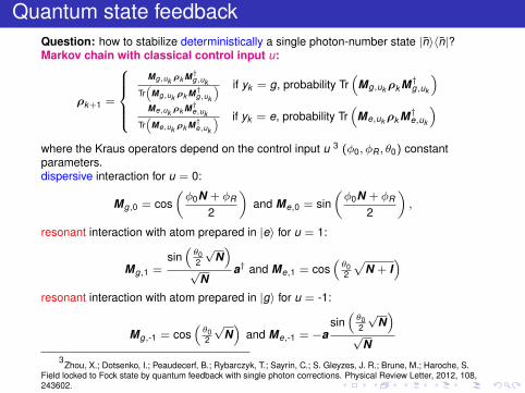
Quantum state feedbackQuestion: how to stabilize deterministically a single photon-number state |n〉〈n|?Markov chain with classical control input u:
ρk+1 =
Mg,uk ρk M†g,uk
Tr(
Mg,uk ρk M†g,uk
) if yk = g, probability Tr(
Mg,uk ρk M†g,uk
)Me,uk ρk M†e,uk
Tr(
Me,uk ρk M†e,uk
) if yk = e, probability Tr(
Me,uk ρk M†e,uk
)where the Kraus operators depend on the control input u 3 (φ0, φR , θ0) constantparameters.dispersive interaction for u = 0:
Mg,0 = cos(φ0N + φR
2
)and Me,0 = sin
(φ0N + φR
2
),
resonant interaction with atom prepared in |e〉 for u = 1:
Mg,1 =sin(θ02
√N)
√N
a† and Me,1 = cos(θ02
√N + I
)resonant interaction with atom prepared in |g〉 for u = -1:
Mg,-1 = cos(θ02
√N)
and Me,-1 = −asin(θ02
√N)
√N
3Zhou, X.; Dotsenko, I.; Peaudecerf, B.; Rybarczyk, T.; Sayrin, C.; S. Gleyzes, J. R.; Brune, M.; Haroche, S.
Field locked to Fock state by quantum feedback with single photon corrections. Physical Review Letter, 2012, 108,243602.

Lyapunov function and quantum-state feedback
Idea: open-loop martingale
V (ρ) = Tr (ρf (N))
with f : [0,+∞[7→ [0,+∞[ strictlydecreasing on [0, n], strictlyincreasing on [n,+∞[ andf (n) = 0 as candidate ofclosed-loop super-martingale withuk function of ρk .
0 2 6 80
0.2
0.4
0.6
0.8
1
4photon number n
Coefficients f(n) of the control Lyapunov function
uk = Γ(ρk ) : = argminu∈-1,0,1
E(V (ρk+1)
∣∣ ρk ,uk = u)
= argminu∈-1,0,1
Tr((
Mg,uρk M†g,u + Me,uρk M†
e,u
)f (N)
)Closed-loop simulations IdealFeedbackPhotonBox.m: truncationto nmax = 7 photons of the Hilbert space, n = 3, f (n) = (n − n)2,φ0 = π/7, φR = 0, θ0 = 2π√
nmax+1.

Cavity decoherence: cavity decay, thermal photon(s)
Three possible outcomes:
zero photon annihilation during ∆T : Kraus operatorM0 = I − ∆T
2 L†−1L−1 − ∆T2 L†1L1, probability ≈ Tr
(M0ρM†0
)with back
action ρt+∆T ≈M0ρt M
†0
Tr(
M0ρM†0) .
one photon annihilation during ∆T : Kraus operator M−1 =√
∆T L−1,
probability ≈ Tr(
M−1ρM†−1
)with back action ρt+∆T ≈
M−1ρt M†−1
Tr(
M−1ρM†−1
)one photon creation during ∆T : Kraus operator M1 =
√∆T L1,
probability ≈ Tr(
M1ρM†1)
with back action ρt+∆T ≈M1ρt M
†1
Tr(
M1ρM†1)
whereL−1 =
√1+nthTcav
a, L1 =√
nthTcav
a†
are the Lindbald operators associated to cavity decoherence : Tcav thephoton life time, ∆T Tcav the sampling period and nth is the average ofthermal photon(s) (vanishes with the environment temperature)( ∆T
Tcav≈ 5× 10⁻⁴, nth ≈ 0.05 for the LKB photon box).

LKB photon-box: controlled Markov process with errors and decoherence
Transition model with control uk from ρk to ρk+1 via ρk+ 12
: measurement back-action
(η ∈ [0, 1] detection error probability and ηeff ∈ [0, 1] detection efficiency)
ρk+ 12
=
(1−η)Mg,uk ρk M†g,uk+ηMe,uk ρk M†e,uk
Tr(
(1−η)Mg,uk ρk M†g,uk+ηMe,uk ρk M†e,uk
) , prob. ηeff Tr(
(1− η)Mg,uk ρk M†g,uk+ ηMe,uk ρk M†e,uk
);
ηMg,uk ρk M†g,uk+(1−η)Me,uk ρk M†e,uk
Tr(ηMg,uk ρk M†g,uk
+(1−η)Me,uk ρk M†e,uk
) prob. ηeff Tr(ηMg,uk ρk M†g,uk
+ (1− η)Me,uk ρk M†e,uk
)Mg,uk ρk M†g,uk
+ Me,uk ρk M†e,ukprob. (1− ηeff )
is completed by cavity decoherence during the small sampling time ∆T :
ρk+1 = M -1ρk+ 12
M†-1 + M0ρk+ 12
M†0 + M1ρk+ 12
M†1.
Model used in simulation to test the robustness of the Lyapunov feedback uk = Γ(ρk )
with η = 1/10, ηeff = 4/10 , ∆TTcav≈ 5× 10⁻⁴ and nth ≈ 0.05

Closed-loop experimental results
Zhou et al. Fieldlocked to Fockstate by quantumfeedback with singlephoton corrections.Physical ReviewLetter, 2012, 108,243602.
See the closed-loop quantum Monte Carlo simulations of the Matlabscript: RealisticFeedbackPhotonBox.m.
Quantum Control1
International Graduate School on Controlwww.eeci-igsc.eu
Pierre Rouchon2
Lecture 11Chengdu, July 11, 2019
1An important part of these slides gathered at the following web pagehave been elaborated with Mazyar Mirrahimi:http://cas.ensmp.fr/~rouchon/ChengduJuly2019/index.html
2Mines ParisTech, INRIA Paris

Outline
1 Reminder: discret-time stochastic master equation
2 Time-continuous stochastic master equations
Discrete-time Stochastic Master Equations (SME)
Trace preserving Kraus map K u depending on the classical control input u:
K u(ρ) =∑µ
Mu,µρM†u,µ with∑µ
M†u,µMu,µ = I .
Take a left stochastic matrix[ηy,µ
](ηy,µ ≥ 0 and
∑y ηy,µ ≡ 1, ∀µ) and set
K u,y (ρ) =∑µ ηy,µMu,µρM†u,µ. The associated Markov chain reads:
ρk+1 =K uk ,yk (ρk )
Tr (K uk ,yk (ρk ))measurement yk with probability Tr (K uk ,yk (ρk )) .
Classical input u, hidden state ρ, measured output y .Ensemble average given by K u since E
(ρk+1
∣∣ ρk , uk)= K uk (ρk ).
Markov model useful for:
1 Monte-Carlo simulations of quantum trajectories (decoherence,measurement back-action).
2 quantum filtering to get the quantum state ρk from ρ0 and (y0, . . . , yk−1)(Belavkin quantum filter developed for diffusive models).
3 feedback design and Monte-Carlo closed-loop simulations.

Outline
1 Reminder: discret-time stochastic master equation
2 Time-continuous stochastic master equations

Markov process under continuous measurement
yt
η
Inverse setup of photon-box: photons read out a qubit.
Two major differences
measurement output taking values from a continuum of possibleoutcomes
dyt =√η Tr
((L + L†)ρt
)dt + dWt .
Time continuous dynamics.

Stochastic master equation: Markov process under continuous measurement
dρt =
(− i~[H,ρt ] +
∑ν
LνρtL†ν −
12(L†νLνρt + ρtL
†νLν)
)dt
+∑ν
√ην
(Lνρt + ρtL
†ν − Tr
((Lν + L†ν)ρt
)ρt
)dWν,t ,
where Wν,t are independent Wiener processes, associated tomeasured signals
dyν,t = dWν,t +√ην Tr
((Lν + L†ν)ρt
)dt .
Wiener process Wt :
W0 = 0;
t →Wt is almost surely everywhere continuous;
For 0 ≤ s1 < t1 ≤ s2 < t2, Wt1 −Ws1 andWt2 −Ws2 areindependent random variables satisfying Wt −Ws ∼ N(0, t − s).
Average dynamics: Lindblad master equation
dE (ρt) =(− i
~ [H,E (ρt)] +∑ν LνE (ρt)L†ν − 1
2 (L†νLνE (ρt) + E (ρt)L†νLν)
)dt .

Ito stochastic calculusGiven a SDE
dXt = F (Xt , t)dt +∑ν
Gν(Xt , t)dWν,t ,
we have the following chain rule:
Ito’s rule
Defining ft = f (Xt) a C2 function of X , we have
dft =
(∂f∂X
∣∣∣Xt
F (Xt , t) +12
∑ν
∂2f∂X 2
∣∣∣Xt
(Gν(Xt , t),Gν(Xt , t))
)dt
+∑ν
∂f∂X
∣∣∣Xt
Gν(Xt , t)dWν,t .
Furthermore
ddt
E (ft) = E
(∂f∂X
∣∣∣Xt
F (Xt , t) +12
∑ν
∂2f∂X 2
∣∣∣Xt
(Gν(Xt , t),Gν(Xt , t))
).

Link to partial Kraus maps (1)
dρt =
(− i~[H,ρt ] +
∑ν
LνρtL†ν −
12(L†νLνρt + ρtL
†νLν)
)dt
+∑ν
√ην
(Lνρt + ρtL
†ν − Tr
((Lν + L†ν)ρt
)ρt
)dWν,t ,
equivalent to
ρt+dt =MdytρtM
†dyt
+∑ν(1− ην)LνρtL
†νdt
Tr(
MdytρtM†dyt
+∑ν(1− ην)LνρtL
†νdt)
withMdyt = I + (− i
~H − 1
2L†νLν)dt +
∑ν
√ηνdyν,tLν .
Moreover, defining dyν,t = sν,t√
dt :
P(st ∈∏ν
[sν , sν + dsν ] | ρt ) =
(Tr(
Ms√
dtρt M†s√
dt
)+∑ν
(1− ην ) Tr(
Lνρt L†ν
)dt
)∏ν
e− |sν |
22 dsν√2π
.

Link to partial Kraus maps (2)
P defines a probability density up to a correction of order dt2:
∫ ∞−∞
. . .
∫ ∞−∞
P
(st ∈
∏ν
[sν , sν + dsν ] | ρt
)∏ν
dsν = 1 + O(dt2).
Mean value of measured signal
∫ ∞−∞
. . .
∫ ∞−∞
sνP
(st ∈
∏ν
[sν , sν + dsν ] | ρt
)∏ν
dsν =√ην Tr
((Lν + L†ν)ρt
)√dt+O(dt3/2).
Variance of measured signal
∫ ∞−∞
. . .
∫ ∞−∞
s2νP
(st ∈
∏ν
[sν , sν + dsν ] | ρt
)∏ν
dsν = 1 + O(dt).
Compatible with dyν,t = sν,t√
dt = dWν,t +√ην Tr
((Lν + L†ν)ρt
)dt .

Link to partial Kraus maps (3)
dρt =
(− i~[H,ρt ] +
∑ν
LνρtL†ν −
12(L†νLνρt + ρtL
†νLν)
)dt
+∑ν
√ην
(Lνρt + ρtL
†ν − Tr
((Lν + L†ν)ρt
)ρt
)dWν,t ,
equivalent to
ρt+dt =MdytρtM
†dyt
+∑ν(1− ην)LνρtL
†νdt
Tr(
MdytρtM†dyt
+∑ν(1− ην)LνρtL
†νdt)
Indicates that the solution remains in the space of semi-definitepositive Hermitian matrices;
Provides a time-discretized numerical scheme preservingnon-negativity of ρ.
Theorem
The above master equation admits a unique solution inρ ∈ CN×N : ρ = ρ†, ρ ≥ 0, Tr (ρ) = 1.

Complements: SME driven by Wiener and Poisson processes
The quantum state ρt is usually mixed and obeys to (measurement outcomes in blue)
dρt =
(−i[H, ρt ] +
∑ν
Lνρt L†ν −
12 (L†νLνρt + ρt L
†νLν ) + Vµρt V
†µ −
12 (V†µVµρt + ρt V
†µVµ)
)dt
+∑ν
√ην
(Lνρt + ρt L
†ν − Tr
((Lν + L†ν )ρt
)ρt
)dWν,t
+∑µ
θµρt +∑µ′ ηµ,µ′Vµρt V
†µ
θµ +∑µ′ ηµ,µ′ Tr
(Vµ′ρt V
†µ′) − ρt
dNµ(t)−
(θµ +
∑µ′ηµ,µ′ Tr
(Vµ′ρt V
†µ′) )
dt
where ην ∈ [0, 1], θµ, ηµ,µ′ ≥ 0 with ηµ′ =∑µ ηµ,µ′ ≤ 1 are parameters modelling measurements
imperfections.
If, for some µ, Nµ(t + dt) − Nµ(t) = 1, we have ρt+dt =θµρt +
∑µ′ ηµ,µ′Vµ′ρt V
†µ′
θµ +∑µ′ ηµ,µ′ Tr
(Vµ′ρt V
†µ′) .
When ∀µ, dNµ(t) = 0, we have
ρt+dt =Mdyt ρt M
†dyt
+∑ν (1− ην )Lνρt L
†νdt +
∑µ(1− ηµ)Vµρt V
†µdt
Tr(
Mdyt ρt M†dyt
+∑ν (1− ην )Lνρt L
†νdt +
∑µ(1− ηµ)Vµρt V
†µdt)
with Mdyt = I +(−iH − 1
2∑ν L†νLν + 1
2∑µ
(ηµ Tr
(Vµρt V
†µ
)I − V†µVµ
))dt +
∑ν√ηνdyνt Lν and
where dyν,t =√ην Tr
((Lν + L†ν ) ρt
)dt + dWν,t .

Quantum Control1
International Graduate School on Controlwww.eeci-igsc.eu
Pierre Rouchon2
Lecture 12Chengdu, July 11, 2019
1An important part of these slides gathered at the following web pagehave been elaborated with Mazyar Mirrahimi:http://cas.ensmp.fr/~rouchon/ChengduJuly2019/index.html
2Mines ParisTech, INRIA Paris

Outline
1 QND measurement of a qubit and asymptotic behavior
2 Exercise: continuous-time QND measurement
Outline
1 QND measurement of a qubit and asymptotic behavior
2 Exercise: continuous-time QND measurement

Dispersive measurement of a qubit
|g〉
|e〉 κ
1
Inverse setup of photon-box: photons read out a qubit.
Approximate model
Cavity’s dynamics are removed (singular perturbation techniques) toachieve a qubit SME:
dρt = − i~
[H,ρt ]dt +Γm
4(σzρtσz − ρt )dt
+
√ηΓm
2(σzρt + ρtσz − 2 Tr (σzρt )ρt )dWt ,
dyt = dWt +√ηΓm Tr (σzρt ) dt .

Quantum Non-Demolition measurement
dρt = − i~
[H,ρt ]dt +Γm
4(σzρtσz − ρt )dt
+
√ηΓm
2(σzρt + ρtσz − 2 Tr (σzρt )ρt )dWt ,
dyt = dWt +√ηΓm Tr (σzρt ) dt .
Uncontrolled case: H/~ = ωegσz/2.
Interpretation as a Markov process with Kraus operators
Mdyt = I −(
iωeg
2σz +
Γm
8I)
dt +
√ηΓm
2σzdyt ,
√(1− η)dtL =
√(1− η)Γmdt
2σz .
QND measurement
Kraus operators Mdyt and√
(1− η)dtL commute with observable σz :qubit states |g〉〈g| and |e〉〈e| are fixed points of the measurementprocess. The measurement is QND for the observable σz .

QND measurement: asymptotic behavior
Theorem
Consider the SME
dρt = − i~
[H,ρt ]dt +Γm
4(σzρtσz − ρt )dt
+
√ηΓm
2(σzρt + ρtσz − 2 Tr (σzρt )ρt )dWt ,
with H =ωeg
2 σz and η > 0.
For any initial state ρ0, the solution ρt converges almost surely ast →∞ to one of the states |g〉〈g| or |e〉〈e|.The probability of convergence to |g〉〈g| (respectively |e〉〈e|) is given bypg = Tr (|g〉〈g|ρ0) (respectively Tr (|e〉〈e|ρ0)).
The convergence rate is given by ηΓM/2.
Proof based on the Lyapunov function V (ρ) =√
Tr (σz 2ρ)− Tr2 (σzρ) with
ddt
E (V (ρ)) = −ηΓM
2E (V (ρ))
Matlab open-loop simulations: RealisticModelQubit.m

Quantum feedback
Question: how to stabilize deterministically a single qubit state |g〉〈g|or |e〉〈e|?Controlled SME:
dρt = − i~
[H,ρt ]dt +Γm
4(σzρtσz − ρt )dt
+
√ηΓm
2(σzρt + ρrσz − 2 Tr (σzρt )ρt )dWt ,
with
H =u(ρt )
2σx +
v(ρt )
2σy ,
u = g sign(Tr (ρσy ))(1− Tr (ρσz )), v = −g sign(Tr (ρσx ))(1− Tr (ρσz ))
stabilizes with gain g > 0 large enough the target state ρtag = |e〉〈e|(based on the control Lyapunov function 1− Tr (ρσz )).
Matlab closed-loop simulations: RealisticFeedbackQubit.m

Exercise: continuous-time QND measurement3
Take a finite dimensional Hilbert spaceH = Cn with the Hermitian operator L of spectral decompositionL =
∑dk=1 λk Πk where λ1, ...λd are the distinct (d ≤ n), real eigenvalues of L with corresponding orthogonal
projection operators Π1, ...,Πd resolving the identity, i.e.∑d
k=1 Πk = I . Assume that the density operator ρ obeysto
dρ =(LρL− (L2
ρ + ρL2)/2)dt +√η(Lρ + ρL− 2 Tr (Lρ) ρ)dW
with diffusive measurement dy = 2√η Tr (Lρ) dt + dW and η > 0.
1 For each k , set pk (ρ) = Tr (ρΠk ). Show that
dpk = 2√η
λk −d∑
k′=1
λk′pk′
pk dW
2 Deduce that ξk =√
pk obeys to
dξk = − 12 η(λk −$(ξ))2
ξk dt +√η(λk −$(ξ))ξk dW ,
with $(ξ) =∑d
k=1 λkξ2k
3 Prove that
d(ξkξk′ ) == − 12 η(λk − λk′ )
2ξk′ξk dt +
√η(λk + λk′ − 2$(ξ))ξkξk′dW .
4 Set V (ρ) =∑
1≤k<k′≤d√
pk (ρ)√
pk′ (ρ). Show that
E(dV | ρ) = − η2∑d
k′=1∑
k′<k (λk − λk′ )2 ξkξk′ dt ≤ − η2
(mink′,k 6=k′ (λk − λk′ )
2)
V (ρ)dt .
5 Conclude that E(V (ρt ) | ρ0) ≤ V (ρ0)e−rt with r > 0 to be defined.3
G. Cardona, A. Sarlette,PR: Exponential stabilization of quantum systems under continuous non-demolitionmeasurements. https://arxiv.org/abs/1906.07403

Quantum Control1
International Graduate School on Controlwww.eeci-igsc.eu
Pierre Rouchon2
Lecture 13Chengdu, July 12, 2019
1An important part of these slides gathered at the following web pagehave been elaborated with Mazyar Mirrahimi:http://cas.ensmp.fr/~rouchon/ChengduJuly2019/index.html
2Mines ParisTech, INRIA Paris
Outline
1 Lindblad master equation
2 Driven and damped qubit
3 Driven and damped harmonic oscillator
4 ComplementsOscillator with thermal photon(s)Wigner function

Outline
1 Lindblad master equation
2 Driven and damped qubit
3 Driven and damped harmonic oscillator
4 ComplementsOscillator with thermal photon(s)Wigner function

The Lindblad master differential equation (finite dimensional case)
ddtρ = − i
~ [H, ρ] +∑ν
LνρL†ν − 1
2 (L†νLνρ+ ρL†
νLν) , L(ρ)
where
H is the Hamiltonian that could depend on t (Hermitian operator on theunderlying Hilbert space H)
the Lν ’s are operators on H that are not necessarily Hermitian.
Qualitative properties (H of finite dimension):
1 Positivity and trace conservation: if ρ0 is a density operator, then ρ(t) remains adensity operator for all t > 0.
2 For any t ≥ 0, the propagator etL is a Kraus map: exists a collection ofoperators (Mµ,t ) such that
∑µ M†
µ,t Mµ,t = I with etL(ρ) =∑µ Mµ,tρM†
µ,t(Kraus theorem characterizing completely positive linear maps).
3 Contraction for many distances such as the nuclear distance: take twotrajectories ρ and ρ′; for any 0 ≤ t1 ≤ t2,
Tr(|ρ(t2)− ρ′(t2)|
)≤ Tr
(|ρ(t1)− ρ′(t1)|
)where for any Hermitian operator A, |A| =
√A2 and Tr (|A|) corresponds to the
sum of the absolute values of its eigenvalues.

Link between Lindblad differential equation and Kraus map
ρk+1 =∑µ
Mµρk M†µ with∑µ
M†µMµ = I
ddt
ρ = − i~ [H,ρ] +
∑ν
LνρL†ν − 12 (L†νLνρ + ρL†νLν)
Take dt > 0 small. Set
Mdt,0 = I − dt
(i~H + 1
2
∑ν
L†νLν
), Mdt,ν =
√dtLν .
Since ρ(t + dt) = ρ(t) + dt( d
dt ρ(t))
+ O(dt2), we have
ρ(t + dt) = Mdt,0ρ(t)M†dt,0 +∑ν
Mdt,νρ(t)M†dt,ν + O(dt2).
Since M†dt,0Mdt,0 +∑ν M†dt,νMdt,ν = I + 0(dt2) the super-operator
ρ 7→ Mdt,0ρM†dt,0 +∑ν
Mdt,νρM†dt,ν
can be seen as an infinitesimal Kraus map.

Outline
1 Lindblad master equation
2 Driven and damped qubit
3 Driven and damped harmonic oscillator
4 ComplementsOscillator with thermal photon(s)Wigner function
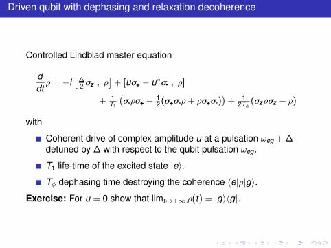
Driven qubit with dephasing and relaxation decoherence
Controlled Lindblad master equation
ddtρ = −i
[∆2 σz , ρ
]+ [uσ+ − u∗σ- , ρ]
+ 1T1
(σ-ρσ+ − 1
2 (σ+σ-ρ+ ρσ+σ-))
+ 12Tφ
(σzρσz − ρ)
with
Coherent drive of complex amplitude u at a pulsation ωeg + ∆detuned by ∆ with respect to the qubit pulsation ωeg .
T1 life-time of the excited state |e〉.
Tφ dephasing time destroying the coherence 〈e|ρ|g〉.
Exercise: For u = 0 show that limt 7→+∞ ρ(t) = |g〉〈g|.
Outline
1 Lindblad master equation
2 Driven and damped qubit
3 Driven and damped harmonic oscillator
4 ComplementsOscillator with thermal photon(s)Wigner function

The driven and damped classical oscillator
Dynamics in the (x ′,p′) phase plane with ω κ,√
u21 + u2
2 :
ddt
x ′ = ωp′,ddt
p′ = −ωx ′ − κp′ − 2u1 sin(ωt) + 2u2 cos(ωt)
Define the frame rotating at ω by (x ′,p′) 7→ (x ,p) with
x ′ = cos(ωt)x + sin(ωt)p, p′ = − sin(ωt)x + cos(ωt)p.
Removing highly oscillating terms (rotating wave approximation), from
ddt
x = −κ sin2(ωt)x + 2u1 sin2(ωt) + (κp − 2u2) sin(ωt) cos(ωt)
ddt
p = −κ cos2(ωt)p + 2u2 cos2(ωt) + (κx − 2u1) sin(ωt) cos(ωt)
we get, with α = x + ip and u = u1 + iu2:
ddtα = −κ2α + u.
With x ′ + ip′ = α′ = e−iωtα, we have ddtα′ = −(κ2 + iω)α′ + ue−iωt

Driven and damped quantum oscillator (nth = 0)
The Lindblad master equation:
ddt
ρ = [ua† − u∗a,ρ] + κ(aρa† − 1
2 a†aρ− 12ρa†a
).
Consider ρ = DαξD−α with α = 2u/κ and Dα = eαa†−α∗a. Weget
ddt
ξ = κ(aξa† − 1
2 a†aξ − 12ξa†a
)since D−αaDα = a + α.
Informal convergence proof with the strict Lyapunov functionV (ξ) = Tr (ξN):
ddt
V (ξ) = −κV (ξ)⇒ V (ξ(t)) = V (ξ0)e−κt .
Since ξ(t) is Hermitian and non-negative, ξ(t) tends to |0〉〈0|when t 7→ +∞.
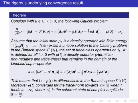
The rigorous underlying convergence result
Theorem
Consider with u ∈ C, κ > 0, the following Cauchy problem
ddt
ρ = [ua† − u∗a,ρ] + κ(aρa† − 1
2 a†aρ− 12ρa†a
), ρ(0) = ρ0.
Assume that the initial state ρ0 is a density operator with finite energyTr (ρ0N) < +∞. Then exists a unique solution to the Cauchy problemin the Banach space K1(H), the set of trace class operators on H. Itis defined for all t > 0 with ρ(t) a density operator (Hermitian,non-negative and trace-class) that remains in the domain of theLindblad super-operator
ρ 7→ [ua† − u∗a,ρ] + κ(aρa† − 1
2 a†aρ− 12ρa†a
).
This means that t 7→ ρ(t) is differentiable in the Banach space K1(H).Moreover ρ(t) converges for the trace-norm towards |α〉〈α| when ttends to +∞, where |α〉 is the coherent state of complex amplitudeα = 2u
κ .

Link with the classical oscillator
Lemma
Consider with u ∈ C, κ > 0, the following Cauchy problem
ddt
ρ = [ua† − u∗a,ρ] + κ(aρa† − 1
2 a†aρ− 12ρa†a
), ρ(0) = ρ0.
1 for any initial density operator ρ0 with Tr (ρ0N) < +∞, we haveddtα = −κ2 (α− α) where α = Tr (ρa) and α = 2u
κ .
2 Assume that ρ0 = |β0〉〈β0| where β0 is some complex amplitude.Then for all t ≥ 0, ρ(t) = |β(t)〉〈β(t)| remains a coherent state ofamplitude β(t) solution of the following equation:ddt β = −κ2 (β − α) with β(0) = β0.
Statement 2 relies on:
a|β〉 = β|β〉, |β〉 = e−ββ∗
2 eβa† |0〉 ddt|β〉 =
(− 1
2 (β∗β + ββ∗) + βa†)|β〉.

Outline
1 Lindblad master equation
2 Driven and damped qubit
3 Driven and damped harmonic oscillator
4 ComplementsOscillator with thermal photon(s)Wigner function

Driven and damped quantum oscillator with thermal photon(s)
Parameters ω κ, |u| and nth > 0:
ddt
ρ = [ua† − u∗a,ρ] + (1 + nth)κ(aρa† − 1
2 a†aρ− 12ρa†a
)+ nthκ
(a†ρa − 1
2 aa†ρ− 12ρaa†
).
Key issue: limt 7→+∞ ρ(t) = ?.With α = 2u/k , we have
ddt
ρ = (1+nth)κ((a − α)ρ(a − α)† − 1
2 (a − α)†(a − α)ρ− 12ρ(a − α)†(a − α)
)+nthκ
((a − α)†ρ(a − α)− 1
2 (a − α)(a − α)†ρ− 12ρ(a − α)(a − α)†
).
Using the unitary change of frame ξ = D−αρDα based on thedisplacement Dα = eαa†−α†a, we get the following dynamics on ξ
ddt
ξ = (1 + nth)κ(aξa† − 1
2 a†aξ − 12ξa†a
)+ nthκ
(a†ξa − 1
2 aa†ξ − 12ξaa†
)since a + α = D−αaDα.
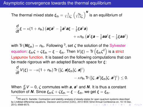
Asymptotic convergence towards the thermal equilibrium
The thermal mixed state ξth = 11+nth
(nth
1+nth
)Nis an equilibrium of
ddt
ξ = κ(1 + nth)(aξa† − 1
2 a†aξ − 12ξa†a
)+ κnth
(a†ξa − 1
2 aa†ξ − 12ξaa†
)with Tr (Nξth) = nth. Following 3, set ζ the solution of the Sylvesterequation: ξthζ + ζξth = ξ − ξth. Then V (ξ) = Tr
(ξthζ
2)
is a strictLyapunov function. It is based on the following computations that canbe made rigorous with an adapted Banach space for ξ:
ddt
V (ξ) = −κ(1 + nth) Tr([ζ,a]ξth[ζ,a]†
)− κnth Tr
([ζ,a†]ξth[ζ,a†]†
)≤ 0.
When ddt V = 0, ζ commutes with a, a† and N . It is thus a constant
function of N . Since ξthζ + ζξth = ξ − ξth, we get ξ = ξth.3
PR and A. Sarlette: Contraction and stability analysis of steady-states for open quantum systems describedby Lindblad differential equations. Decision and Control (CDC), 2013 IEEE 52nd Annual Conference on, 10-13 Dec.2013, 6568-6573.

Outline
1 Lindblad master equation
2 Driven and damped qubit
3 Driven and damped harmonic oscillator
4 ComplementsOscillator with thermal photon(s)Wigner function
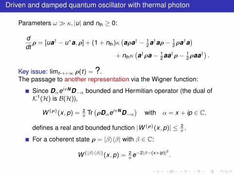
Driven and damped quantum oscillator with thermal photon
Parameters ω κ, |u| and nth ≥ 0:
ddt
ρ = [ua† − u∗a,ρ] + (1 + nth)κ(aρa† − 1
2 a†aρ− 12ρa†a
)+ nthκ
(a†ρa − 1
2 aa†ρ− 12ρaa†
).
Key issue: limt 7→+∞ ρ(t) = ?.The passage to another representation via the Wigner function:
Since DαeiπND−α bounded and Hermitian operator (the dual ofK1(H) is B(H)),
W ρ(x ,p) = 2π Tr
(ρDαeiπND−α
)with α = x + ip ∈ C,
defines a real and bounded function |W ρ(x ,p)| ≤ 2π .
For a coherent state ρ = |β〉〈β| with β ∈ C:
W |β〉〈β|(x ,p) = 2πe−2|β−(x+ip)|2 .

The partial differential equation satisfied by the Wigner function (1)
With Dα = eαa†e−α∗ae−αα
∗/2 = e−α∗aeαa†eαα
∗/2 we have:
π2 W ρ(α, α∗) = Tr
(ρeαa†e−α
∗aeiπNeα∗ae−αa†
)where α and α∗ are seen as independent variables:
∂
∂α= 1
2
(∂
∂x− i
∂
∂p
),
∂
∂α∗= 1
2
(∂
∂x+ i
∂
∂p
)We have π
2∂∂αW ρ(α, α∗) = Tr
((ρa† − a†ρ)DαeiπND−α
)Since
a†DαeiπND−α = DαeiπND−α(2α∗ − a†), we get
∂
∂αW ρ(α, α∗) = 2α∗W ρ(α, α∗)− 2W a†ρ(α, α∗).
Thus W a†ρ(α, α∗) = α∗W ρ(α, α∗)− 12∂∂αW ρ(α, α∗), i.e.
W a†ρ =
(α∗ − 1
2∂
∂α
)W ρ.

The partial differential equation satisfied by the Wigner function (2)
Similar computations yield to the following correspondence rules:
W ρa =
(α− 1
2∂
∂α∗
)W ρ, W aρ =
(α + 1
2∂
∂α∗
)W ρ
W ρa† =
(α∗ + 1
2∂
∂α
)W ρ, W a†ρ =
(α∗ − 1
2∂
∂α
)W ρ.
Thus
ddt
ρ = [ua† − u∗a,ρ] + (1 + nth)κ(aρa† − 1
2 a†aρ− 12ρa†a
)+ nthκ
(a†ρa − 1
2 aa†ρ− 12ρaa†
).
becomes
∂
∂tW ρ =
κ
2
(∂
∂α(α− α) +
∂
∂α∗(α∗ − α∗) + (1 + 2nth)
∂2
∂α∂α∗
)W ρ
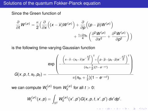
Solutions of the quantum Fokker-Planck equation
Since the Green function of
∂
∂tW ρ =
κ
2
( ∂
∂x
((x − x)W ρ
)+
∂
∂p
((p − p)W ρ
)+ 1+2nth
4
(∂2W ρ
∂x2 +∂2W ρ
∂p2
))is the following time-varying Gaussian function
G(x ,p, t , x0,p0) =
exp
−(
x−x−(x0−x)e−κt2
)2
+
(p−p−(p0−p)e−
κt2
)2
(nth+12 )(1−e−κt )
π(nth + 1
2 )(1− e−κt )
we can compute W ρt from W ρ
0 for all t > 0:
W ρt (x ,p) =
∫R2
W ρ0 (x ′,p′)G(x ,p, t , x ′,p′) dx ′dp′.

Asymptotics of the quantum Fokker-Planck equation
Combining
W ρt (x ,p) =
∫R2 W ρ
0 (x ′,p′)G(x ,p, t , x ′,p′) dx ′dp′.
G uniformly bounded and
limt 7→+∞G(x ,p, t , x ′,p′) = 1
π(nth+12 )
exp(− (x−x)2+(p−p)2
(nth+12 )
)W ρ
0 in L1 with∫∫
R2 W ρ0 = 1
dominate convergence theorem
shows that all the solutions converge to a unique steady-stateGaussian density function, centered in (x ,p) with variance 1
2 + nth:
∀(x ,p) ∈ R2, limt 7→+∞
W ρt (x ,p) = 1
π(nth+12 )
exp
(− (x − x)2 + (p − p)2
(nth + 12 )
).

Quantum Control1
International Graduate School on Controlwww.eeci-igsc.eu
Pierre Rouchon2
Lecture 14Chengdu, July 12, 2019
1An important part of these slides gathered at the following web pagehave been elaborated with Mazyar Mirrahimi:http://cas.ensmp.fr/~rouchon/ChengduJuly2019/index.html
2Mines ParisTech, INRIA Paris

Outline
1 Coherent feedback stabilisation
2 Slow measurement-based feedback
Outline
1 Coherent feedback stabilisation
2 Slow measurement-based feedback

Coherent (autonomous) feedback (dissipation engineering)
Quantum analogue of Watt speed governor: a dissipativemechanical system controls another mechanical system 3
system
controller
quantum world
classical world
decoherence
decoherence
uy
uc yc
Optical pumping (Kastler 1950), coherentpopulation trapping (Arimondo 1996)
Dissipation engineering, autonomousfeedback: (Zoller, Cirac, Wolf, Verstraete,Devoret, Schoelkopf, Siddiqi, Lloyd, Viola,Ticozzi, Leghtas, Mirrahimi, Sarlette, ...)
(S,L,H) theory and linear quantumsystems: quantum feedback networksbased on stochastic Schrödinger equation,Heisenberg picture (Gardiner, Yurke,Mabuchi, Genoni, Serafini, Milburn,Wiseman, Doherty, Gough, James,Petersen, Nurdin, Yamamoto, Zhang,Dong, . . . )
Stability analysis: Kraus maps and Lindblad propagators are alwayscontractions (non commutative diffusion and consensus).
3J.C. Maxwell: On governors. Proc. of the Royal Society, No.100, 1868.

Coherent feedback underlying the cat-qubit (1) 4
System: high quality oscillator with annihilation operator a:
ddtρ = −iωa[a†a, ρ] + κa
(aρa† − 1
2 (a†aρ+ ρa†a)).
Controller: low quality oscillator κa κb with annihilation operator b with resonantdrive
ddtρ = −iωb[b†b, ρ] + [−ueiωb t b† + u∗e−iωb t b, ρ] + κb
(bρb† − 1
2 (b†bρ+ ρb†b)).
Coupling Hamiltonian term g[a2b† − (a†)2b, ρ] yields to the closed-loop Lindbladequation
ddtρ = −i[ωaa†a + ωbb†b] + [−ue−iωb t b† + u∗e+iωb t b, ρ] + g[a2b† − (a†)2b, ρ]
+ κa
(aρa† − 1
2 (a†aρ+ ρa†a))
+ κb
(bρb† − 1
2 (b†bρ+ ρb†b))
4M. Mirrahimi, Z. Leghtas, . . . , M.H. Devoret: Dynamically protectedcat-qubits: a new paradigm for universal quantum computation.New Journalof Physics,2014, 16:045014.

Coherent feedback underlying the cat-qubit (2)
• For ωb = 2ωa one gets in the the frame rotating at ωa for mode a and ωb for mode b(unitary transformation: ρold = e−iωa ta†a−iωb tb†bρnew eiωa ta†a+iωb tb†b):
ddtρ = g
[(a2 − u
g )b† − ((a†)2 − u∗g )b, ρ
]+ κa
(aρa† − 1
2 (a†aρ+ ρa†a))
+ κb
(bρb† − 1
2 (b†bρ+ ρb†b)).
• If we neglect κa in front of κb , any ρ of the form ρ = ρa ⊗ |0b〉〈0b| with ρa densityoperator on mode a with support in span|α〉, |-α〉 where α =
√ug ∈ C, is a
steady-state of the above Lindbald equation with κa = 0.
• If additionally, g κb , the strongly damped mode b can be eliminated via singularperturbation techniques (quasi-static or adiabatic approximation) to get the followingslow Lindblad equation on mode a only:
ddtρ = 4g2
κb
(LρL† − 1
2 (L†Lρ+ ρL†L))
+ κa
(aρa† − 1
2 (a†aρ+ ρa†a))
with Lindblad operator L = a2 − α2.

Coherent feedback underlying the cat-qubit (3)
• If g √κaκb then we can still neglect κa. Any solution of
ddtρ = 4g2
κb
(LρL† − 1
2 (L†Lρ+ ρL†L))
converges to a steady state ρa with support in span|α〉, |-α〉 (use the Lyapunovfunction V (ρ) = Tr
(LρL†
) 5).
• For ddt ρ = 4g2
κb
(LρL† − 1
2 (L†Lρ+ ρL†L))
+ κa
(aρa† − 1
2 (a†aρ+ ρa†a))
withg √κaκb , a reduction to the sub-space span|α〉, |-α〉 is possible to describe thevery slow evolution due to κa. With the orthonormal basis,
|c+α 〉 = |α〉+|-α〉√
2(1+e−2|α|2 )(even cat) and |c-
α〉 = |α〉−|-α〉√2(1−e−2|α|2 )
(odd cat),
define the swap operator Xc = |c+α 〉〈c-
α|+ |c-α〉〈c+
α |. Since a|c+α 〉 = α|c-
α〉 anda|c-
α〉 = α|c+α 〉, the reduced dynamics on Hc , span|c+
α 〉, |c-α〉 reads
ddtρc = κa|α|2(XcρcXc − ρc)
where ρc a density operator on Hc .5
R. Azouit, A. Sarlette, and PR: Well-posedness and convergence of the Lindblad master equation for aquantum harmonic oscillator with multi-photon drive and damping. ESAIM: COCV, 2016, 22(4):1353 –1369.

Outline
1 Coherent feedback stabilisation
2 Slow measurement-based feedback

Final slow measurement-based feedback stabilisation
Assume that one can continuously and weakly measure the parity eiπa†a of mode awith a rate γa κa|α|2. Then we have the following stochastic master equation(Zc = |c+
α 〉〈c+α | − |c
−α 〉〈c−α |)
dρc = κa|α|2(XcρcXc−ρc)dt+γa(ZcρcZc−ρc)dt+√ηcγa(Zcρc+ρcZc−2 Tr (Zcρc) ρc)dW
with continuous-time measurement output yc of efficiency ηc > 0 and given bydyc = 2
√ηcγa Tr (Zcρc) dt + dW .
One can stabilize either |c+α 〉〈c+
α | or |c−α 〉〈c−α | if we have at our disposal a classicalinput signal uc attached to an Hamiltonian Hc on Hc independent of Zc .
Exercise: design a measurement-based feedback stabilizing |c+α 〉〈c+
α | with Hc = Xc
and based on the Lyapunov function Vc(ρc) =√〈c+α |ρc |c+
α 〉 for κa = 0. Analyse theimpact of κa > 0 with closed-loop Monte-Carlo simulations.
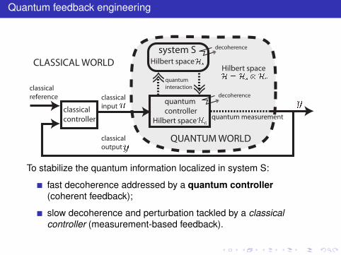
Quantum feedback engineering
QUANTUM WORLD
CLASSICAL WORLDHilbert space
classical controller
quantum controllerHilbert space
Hilbert space system S
decoherence
decoherence
classicalinput
classicaloutput
quantum measurement
classicalreference
quantuminteraction
To stabilize the quantum information localized in system S:
fast decoherence addressed by a quantum controller(coherent feedback);
slow decoherence and perturbation tackled by a classicalcontroller (measurement-based feedback).