Quantum computation of ﬂuid dynamics

Indian Academy of Sciences Conference Series (2020) 3:1DOI: 10.29195/iascs.03.01.0015

© Indian Academy of Sciences

Quantum computation of fluid dynamics

SACHIN S. BHARADWAJ1 and KATEPALLI R. SREENIVASAN1,2,3,4,∗

1 Department of Mechanical and Aerospace Engineering, New York University, New York, 11201, USA2 Department of Physics, New York University, New York, 10012, USA3 Courant Institute of Mathematical Sciences, New York University, New York, 10012, USA4 New York University, Abu Dhabi, 129188, UAE∗Corresponding author. E-mail: [email protected]

Abstract. Studies of strongly nonlinear dynamical systems such as turbulent flows call for superior computationalprowess. With the advent of quantum computing (QC), a plethora of quantum algorithms have demonstrated,both theoretically and experimentally, more powerful computational possibilities than their classical counterparts.Starting with a brief introduction to QC, we will distill a few key tools and algorithms from the huge spectrum ofmethods available and evaluate possible approaches of QC in fluid dynamics.

Keywords. Quantum computing; fluid dynamics; nonlinear dynamics; turbulence simulations.

PACS Nos 12.60.Jv; 12.10.Dm; 98.80.Cq; 11.30.Hv

1. Introduction

Fluid mechanics as a field poses a vast array of inter-esting questions that relate to almost everything we seearound us. Apart from theory and experiments, com-putational methods have greatly aided fluid mechan-ics research over the past few decades; indeed, withthe growth in computers of increasingly higher com-putational power, fluid mechanical simulations havebecome highly realistic. But with increasing sophistica-tion comes new generations of questions. For instance,even with the great advances seen in high performancecomputing (HPC), and despite the progress being madecontinually by very large direct numerical simulations(DNS), one cannot say that long-standing questionsrelating to the separation of scales in turbulence havebeen addressed fully. Without necessarily making theexplicit case that computer technology developmenthas hit obstacles, we simply note that the computa-tional challenges being faced at present are so enormousthat simply making supercomputers more powerful can-not catch up with the demands. Not only manufactur-ing smaller transistors face quantum effects but alsotheir integration into massively complex systems posesnumerous challenges. To break this barrier, one needsa change of paradigm in computing. Enter quantumcomputing (QC)!

In QC, we manipulate quantum systems to performcalculations and simulations. We are thus entering an

era in which computations are becoming more ‘physi-cal’. In fact, it was a dream of Feynman [1] to simulatea quantum system by using another quantum system.We are now in the noisy intermediate scale quantum(NISQ) era [2], where we have quantum computersof sizes ranging from 50 qubits to a few hundreds ofthem. (Qubits are essentially the quantum analogue ofclassical bits and will be described later; it sufficesto say here that their number characterizes the powerand size of a quantum computer.) The word ‘noisy’indicates that quantum devices are still prone to errorsfrom external and internal noises and are not yet per-fect. Yet, with quantum devices of the size just emerg-ing, QC can outperform many operations that currentsupercomputers strain to achieve. Quantum computershave already started demonstrating their practicabilityin various fields such as finance strategies, medicine,quantum materials and chemical simulations, resourcemanagement, optimization and cryptography. What wewish to investigate here is its utility for performingcomputational fluid dynamics (CFD) research.

This paper presents an outlook on doing CFD quan-tum mechanically, which we term quantum computationof fluid dynamics (QCFD). It introduces and moti-vates researchers who wish to study fluid mechanicsor dynamical systems, in general, to the new possibilityof using quantum computers. In section 2, we presenta brief overview of QC and its differences from clas-sical computing. We then set up in section 3 the big

78 Indian Academy of Sciences Conference Series (2020) 3:1

picture of how fluid mechanics study can be viewed inthe QC context. This is followed by a description ofmethods that are lattice based (section 4) and contin-uum based (section 5). Section 5 also touches on thepossibility of studying quantum turbulence and reviewsexistent methods and proposes newer directions. Insection 6, we list from the horde of QC algorithms afew key ones that are deemed important for our purposesand provide a few specific demonstrations. Finally, webriefly mention in section 7 the currently available quan-tum machines and quantum programming, ending witha few conclusions on QCFD in section 7.

2. Overview of quantum computation

The purpose of this section is to provide a brief overviewof how the working rules of QC differ from those of clas-sical computing. It is intended for readers with minimalbackground in QC; a detailed account can be found inRef. [3].

2.1 What is quantum computation?

It is a form of computation centered on quantummechanics, manipulating information in the form ofquantum bits called ‘qubits’, by designing appropriate‘quantum algorithms’ that comprise ‘quantum gates andcircuits’, which in turn act on these qubits to yield theintended result. This sounds similar to classical com-putation, except that every word or phrase is prefixedby the word ‘quantum’. We shall explain each of theseterms below.

2.2 Qubits

Qubits form the work horse of quantum computation.Similar to classical bits, quantum bits are objects thathold information describing quantum physical systems,which are eventually manipulated to perform a com-putational task. In reality, these qubits represent thestate of an actual quantum physical system, governedby laws of quantum mechanics. Mathematically, it isgiven by the wavefunctionΨ, which completely encodesall the details describing the state of a quantum object.As a working example, a qubit could represent the twospin states of an electron. There exist several physicalrealizations of qubits such as quantum electro-dynamic(QED) optical cavities, ultra cold atoms and Rydbergions, superconductors and topological materials (Majo-rana fermions), photons, quantum dots, nuclear mag-netic resonance (NMR), etc. For the rest of the paper,however, we shall simply describe qubits as abstractmathematical objects. For now and for all practical pur-poses, we shall denote qubits as wavefunctions, whichare vectors in a complex vector space called the Hilbert

space H. In Dirac’s bra–ket notation, it is represented asa ‘ket’ vector |Ψ〉 in H (∈ Cn)

|ψ〉 =

c1

c2...

cn

; ci ∈ C (1)

while ‘bra’, given by 〈Ψ|, is the vector dual = |Ψ〉�.These wavefunctions obey all the rules of a complexvector space. An obvious extension to this concept isto multiple qubits by taking tensor products of indi-vidual wavefunctions, which together lie in a tensor-product Hilbert space of the corresponding wavefunc-tions: |Ψ〉 = (|ψ1〉⊗· · ·⊗|ψn〉) ∈ H⊗n. For instance, thetwo spin states (spin-up ↑ and spin-down ↓) of an elec-tron, could correspond to the state eigenvectors |0〉 and|1〉, respectively. The wavefunction of such two level ortwo state systems is a complex vector inH ∈ C⊗2 which,when expressed mathematically as a linear combinationof the basis vectors, has the form

|Ψ〉 = c1|0〉 + c2|1〉, (2)

where

0〉 =[10

]and |1〉 =

[01

]. (3)

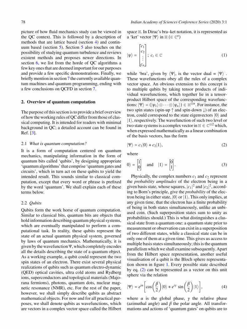
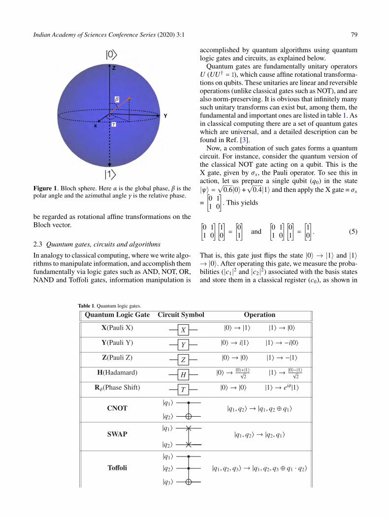
Physically, the complex numbers c1 and c2 representthe probability amplitudes of the electron being in agiven basis state, whose squares, |c1|2 and |c2|2, accord-ing to Born’s principle, give the probability of the elec-tron being in either state, |0〉 or |1〉. This only implies, atany given time, that the electron has a finite probabilityof being in both states simultaneously, unlike an unbi-ased coin. (Such superposition states sum to unity asprobabilities should.) This is what distinguishes a clas-sical state from a quantum one: a quantum state prior tomeasurement or observation can exist in a superpositionof two different states, while a classical state can be inonly one of them at a given time. This gives us access tomultiple basis states simultaneously; this is the quantumparallelism which we shall examine subsequently. Apartfrom the Hilbert space representation, another usefulvisualisation of a qubit is the Bloch sphere representa-tion shown in figure 1. Every possible state describedby eq. (2) can be represented as a vector on this unitsphere via the relation

|Ψ〉 = eiα[

cos(β2

)|0〉 + eiγ sin

(β2

)|1〉]

, (4)

where α is the global phase, γ the relative phase(azimuthal angle) and β the polar angle. All transfor-mations and actions of ‘quantum gates’ on qubits are to

Indian Academy of Sciences Conference Series (2020) 3:1 79

Figure 1. Bloch sphere. Here α is the global phase, β is thepolar angle and the azimuthal angle γ is the relative phase.

be regarded as rotational affine transformations on theBloch vector.

2.3 Quantum gates, circuits and algorithms

In analogy to classical computing, where we write algo-rithms to manipulate information, and accomplish themfundamentally via logic gates such as AND, NOT, OR,NAND and Toffoli gates, information manipulation is

accomplished by quantum algorithms using quantumlogic gates and circuits, as explained below.

Quantum gates are fundamentally unitary operatorsU (UU† = I), which cause affine rotational transforma-tions on qubits. These unitaries are linear and reversibleoperations (unlike classical gates such as NOT), and arealso norm-preserving. It is obvious that infinitely manysuch unitary transforms can exist but, among them, thefundamental and important ones are listed in table 1. Asin classical computing there are a set of quantum gateswhich are universal, and a detailed description can befound in Ref. [3].

Now, a combination of such gates forms a quantumcircuit. For instance, consider the quantum version ofthe classical NOT gate acting on a qubit. This is theX gate, given by σx, the Pauli operator. To see this inaction, let us prepare a single qubit (q0) in the state|ψ〉 =

√0.6|0〉+

√0.4|1〉 and then apply the X gate = σx

=

[0 11 0

]. This yields

[0 11 0

][10

]=[01

]and

[0 11 0

][01

]=[10

]. (5)

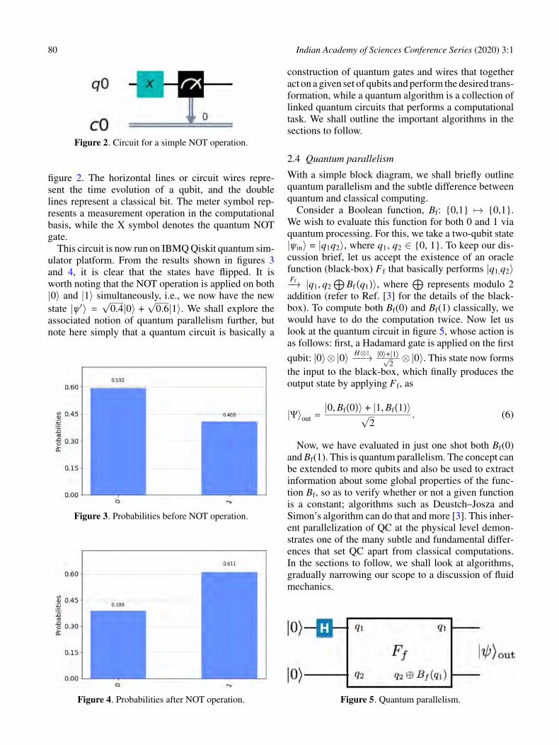
That is, this gate just flips the state |0〉 → |1〉 and |1〉→ |0〉. After operating this gate, we measure the proba-bilities (|c1|2 and |c2|2) associated with the basis statesand store them in a classical register (c0), as shown in

Table 1. Quantum logic gates.


Figure 2. Circuit for a simple NOT operation.

figure 2. The horizontal lines or circuit wires repre-sent the time evolution of a qubit, and the doublelines represent a classical bit. The meter symbol rep-resents a measurement operation in the computationalbasis, while the X symbol denotes the quantum NOTgate.

This circuit is now run on IBMQ Qiskit quantum sim-ulator platform. From the results shown in figures 3and 4, it is clear that the states have flipped. It isworth noting that the NOT operation is applied on both|0〉 and |1〉 simultaneously, i.e., we now have the newstate |ψ′〉 =

√0.4|0〉 +

√0.6|1〉. We shall explore the

associated notion of quantum parallelism further, butnote here simply that a quantum circuit is basically a

Figure 3. Probabilities before NOT operation.

Figure 4. Probabilities after NOT operation.

construction of quantum gates and wires that togetheract on a given set of qubits and perform the desired trans-formation, while a quantum algorithm is a collection oflinked quantum circuits that performs a computationaltask. We shall outline the important algorithms in thesections to follow.

2.4 Quantum parallelism

With a simple block diagram, we shall briefly outlinequantum parallelism and the subtle difference betweenquantum and classical computing.

Consider a Boolean function, Bf: {0,1} 7→ {0,1}.We wish to evaluate this function for both 0 and 1 viaquantum processing. For this, we take a two-qubit state|ψin〉 = |q1q2〉, where q1, q2 ∈ {0, 1}. To keep our dis-cussion brief, let us accept the existence of an oraclefunction (black-box) Ff that basically performs |q1,q2〉Ff−→ |q1, q2

⊕Bf (q1)〉, where

⊕represents modulo 2

addition (refer to Ref. [3] for the details of the black-box). To compute both Bf(0) and Bf(1) classically, wewould have to do the computation twice. Now let uslook at the quantum circuit in figure 5, whose action isas follows: first, a Hadamard gate is applied on the first

qubit: |0〉⊗ |0〉 H⊗I−−→ |0〉+|1〉√2⊗|0〉. This state now forms

the input to the black-box, which finally produces theoutput state by applying Ff, as

|Ψ〉out =|0, Bf(0)〉 + |1, Bf(1)〉√

2. (6)

Now, we have evaluated in just one shot both Bf(0)and Bf(1). This is quantum parallelism. The concept canbe extended to more qubits and also be used to extractinformation about some global properties of the func-tion Bf, so as to verify whether or not a given functionis a constant; algorithms such as Deustch–Josza andSimon’s algorithm can do that and more [3]. This inher-ent parallelization of QC at the physical level demon-strates one of the many subtle and fundamental differ-ences that set QC apart from classical computations.In the sections to follow, we shall look at algorithms,gradually narrowing our scope to a discussion of fluidmechanics.

Figure 5. Quantum parallelism.


3. QC of dynamical systems: The big picture

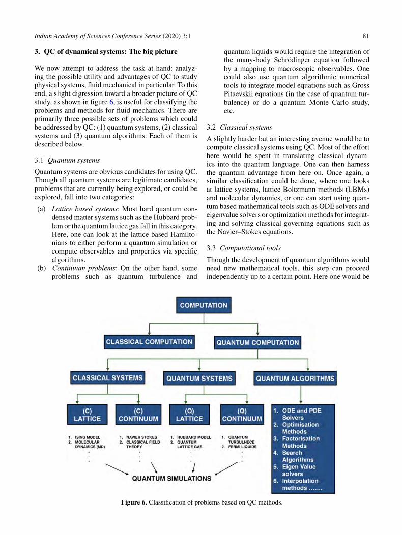
We now attempt to address the task at hand: analyz-ing the possible utility and advantages of QC to studyphysical systems, fluid mechanical in particular. To thisend, a slight digression toward a broader picture of QCstudy, as shown in figure 6, is useful for classifying theproblems and methods for fluid mechanics. There areprimarily three possible sets of problems which couldbe addressed by QC: (1) quantum systems, (2) classicalsystems and (3) quantum algorithms. Each of them isdescribed below.

3.1 Quantum systems

Quantum systems are obvious candidates for using QC.Though all quantum systems are legitimate candidates,problems that are currently being explored, or could beexplored, fall into two categories:

(a) Lattice based systems: Most hard quantum con-densed matter systems such as the Hubbard prob-lem or the quantum lattice gas fall in this category.Here, one can look at the lattice based Hamilto-nians to either perform a quantum simulation orcompute observables and properties via specificalgorithms.

(b) Continuum problems: On the other hand, someproblems such as quantum turbulence and

quantum liquids would require the integration ofthe many-body Schrödinger equation followedby a mapping to macroscopic observables. Onecould also use quantum algorithmic numericaltools to integrate model equations such as GrossPitaevskii equations (in the case of quantum tur-bulence) or do a quantum Monte Carlo study,etc.

3.2 Classical systems

A slightly harder but an interesting avenue would be tocompute classical systems using QC. Most of the efforthere would be spent in translating classical dynam-ics into the quantum language. One can then harnessthe quantum advantage from here on. Once again, asimilar classification could be done, where one looksat lattice systems, lattice Boltzmann methods (LBMs)and molecular dynamics, or one can start using quan-tum based mathematical tools such as ODE solvers andeigenvalue solvers or optimization methods for integrat-ing and solving classical governing equations such asthe Navier–Stokes equations.

3.3 Computational tools

Though the development of quantum algorithms wouldneed new mathematical tools, this step can proceedindependently up to a certain point. Here one would be

Figure 6. Classification of problems based on QC methods.


interested primarily in developing, quantum mechan-ically, the numerical solvers or methods available onclassical machines, such as optimization, ODE/PDEsolvers, factorizations, data search, eigenvalue solvers,etc.

With this background, we now proceed to examineeach of these methods and provide real quantum compu-tational demonstrations. From these methods, we shallfocus primarily on two methods suitable for studyingfluid dynamics: (1) lattice based methods and (2) con-tinuum quantum simulations and quantum algorithms.

4. Lattice simulations

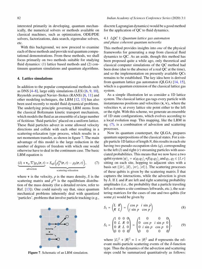
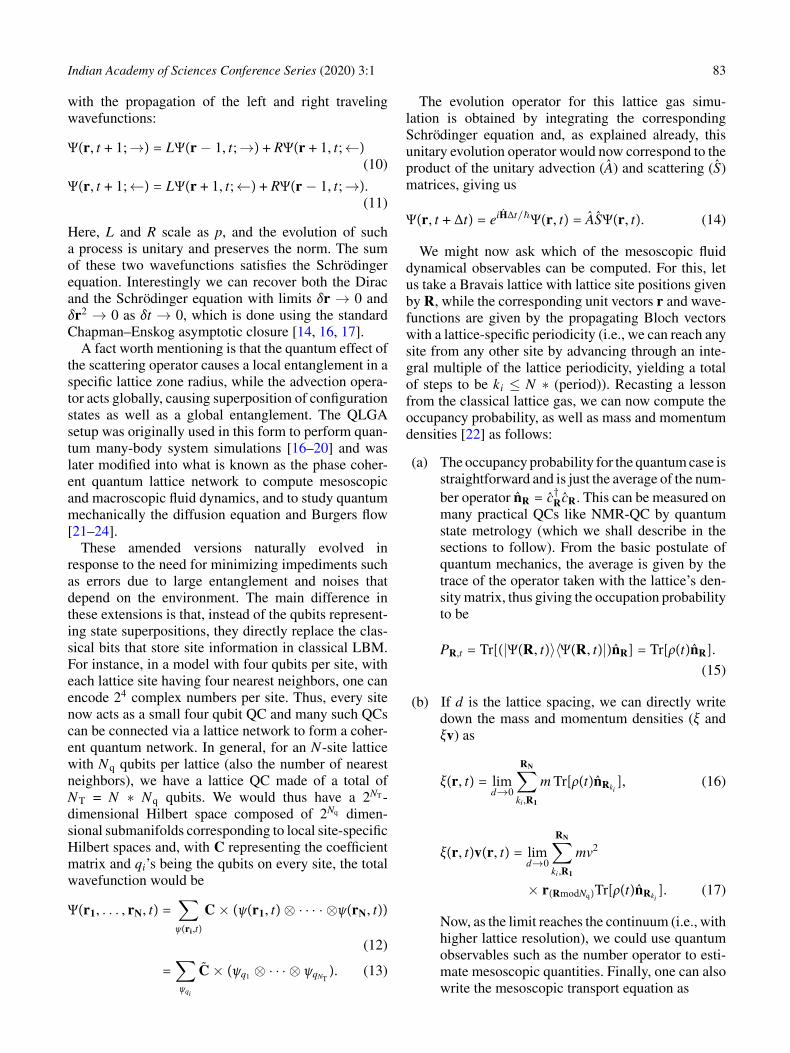
In addition to the popular computational methods suchas DNS [4–8], large eddy simulations (LES) [6, 9, 10],Reynolds averaged Navier–Stokes (RANS) [6, 11] andother modeling techniques, the LBM [12, 13] has alsobeen used recently to model fluid dynamical problems.The underlying principle governing LBM stems fromthe classical Boltzmann kinetic transport mechanism,which models the fluid as an ensemble of a large numberof fictitious ‘fluid particles’ placed on a uniform lattice.These fluid particles advect in some allowed velocitydirections and collide with each other resulting in ascattering-relaxation type process, which results in anet momentum transfer, as shown in figure 7. The mainadvantage of this model is the large reduction in thenumber of degrees of freedom with which one wouldotherwise have to deal in the continuum case. The basicLBM equation is

(∂t + vα.∇)ρα(r, t)︸︷︷︸advection

= Sαβ(ρeqβ (r, t)− ρβ(r, t)

)︸︷︷︸

scattering-relaxation

, (7)

where v is the velocity, ρ is the mass density, S is thescattering matrix and ρeq is the equilibrium distribu-tion of the mass density (for a detailed review, refer toRef. [13]). One could naively say that, since quantummechanical problems inherently deal with quantized‘particles’, problems that involve particle tracking (e.g.,

Figure 7. Schematic of an LBM simulation.

discrete Lagrangian dynamics) would be a good methodfor the application of QC to fluid dynamics.

4.1 LQC 1: Quantum lattice gas automatonand phase coherent quantum networks

This method provides insights into one of the physicalframeworks for generating a map from classical fluiddynamics to QC. As an aside, though this method hasbeen proposed quite a while ago, only theoretical andclassical computer simulations of the QC method hadbeen done (due to the absence of a real QC at the time),and so the implementation on presently available QCsremains to be established. The key idea here is derivedfrom quantum lattice gas automaton (QLGA) [14, 15],which is a quantum extension of the classical lattice gassystem.

As a simple illustration let us consider a 1D latticesystem. The classical lattice gas tags every particle withinstantaneous positions and velocities (x, v)i, where thevelocities vi at every lattice site point either to the leftor the right. With this scheme, we generate an ensembleof 1D state configurations, which evolves according toa local evolution map. This mapping, like the LBM ineq. (7), is a combination of advection and scatteringprocesses.

Now its quantum counterpart, the QLGA, preparesquantum superpositions of the classical states. For a sin-gle particle 1D lattice of length N, this results in each sitehaving two pseudo-occupation slots (q), correspondingto the left (l) and right (r) streaming particles with asso-ciated probabilities. This means that we now have a twoqubit system |ψ〉i = α|q1q2〉i+β|q1q2〉i and q1, q2∈ {l, r}sitting on each site, hopping to adjacent sites with abasis set {|lr〉, |ll〉, |rr〉, |rl〉}. The scattering processesof these qubits is given by the scattering matrix S thatcaptures the interactions, while the advection is givenby A. If L and R are left and right scattering probabilityamplitudes (i.e., the probability that a particle travelingleft as it enters a site continues leftwards, etc.), the scat-tering matrices for the cases of one and two qubits (forsome p) would be given by

S1 =(

L RR L

)=(

cos p i sin pi sin p cos p

)(8)

S2 =

1 0 0 00 L R 00 R L 00 0 0 θ

=

1 0 0 00 cos p i sin p 00 i sin p cos p 00 0 0 θ

, (9)

where |L|2 + |R|2 = 1 = |θ|2 and θ represents the rel-evant multi-particle scattering events of the δ-functiontype. Thus the dynamics of the advection and scatteringsteps could be summarized quantitatively as follows:


with the propagation of the left and right travelingwavefunctions:

Ψ(r, t + 1;→) = LΨ(r − 1, t;→) + RΨ(r + 1, t;←)(10)

Ψ(r, t + 1;←) = LΨ(r + 1, t;←) + RΨ(r − 1, t;→).(11)

Here, L and R scale as p, and the evolution of sucha process is unitary and preserves the norm. The sumof these two wavefunctions satisfies the Schrödingerequation. Interestingly we can recover both the Diracand the Schrödinger equation with limits δr → 0 andδr2 → 0 as δt → 0, which is done using the standardChapman–Enskog asymptotic closure [14, 16, 17].

A fact worth mentioning is that the quantum effect ofthe scattering operator causes a local entanglement in aspecific lattice zone radius, while the advection opera-tor acts globally, causing superposition of configurationstates as well as a global entanglement. The QLGAsetup was originally used in this form to perform quan-tum many-body system simulations [16–20] and waslater modified into what is known as the phase coher-ent quantum lattice network to compute mesoscopicand macroscopic fluid dynamics, and to study quantummechanically the diffusion equation and Burgers flow[21–24].

These amended versions naturally evolved inresponse to the need for minimizing impediments suchas errors due to large entanglement and noises thatdepend on the environment. The main difference inthese extensions is that, instead of the qubits represent-ing state superpositions, they directly replace the clas-sical bits that store site information in classical LBM.For instance, in a model with four qubits per site, witheach lattice site having four nearest neighbors, one canencode 24 complex numbers per site. Thus, every sitenow acts as a small four qubit QC and many such QCscan be connected via a lattice network to form a coher-ent quantum network. In general, for an N-site latticewith Nq qubits per lattice (also the number of nearestneighbors), we have a lattice QC made of a total ofNT = N ∗ Nq qubits. We would thus have a 2NT -dimensional Hilbert space composed of 2Nq dimen-sional submanifolds corresponding to local site-specificHilbert spaces and, with C representing the coefficientmatrix and qi’s being the qubits on every site, the totalwavefunction would be

Ψ(r1, . . . , rN, t) =∑ψ(ri,t)

C× (ψ(r1, t)⊗ · · · · ⊗ψ(rN, t))

(12)

=∑ψqi

C× (ψq1 ⊗ · · · ⊗ ψqNT). (13)

The evolution operator for this lattice gas simu-lation is obtained by integrating the correspondingSchrödinger equation and, as explained already, thisunitary evolution operator would now correspond to theproduct of the unitary advection (A) and scattering (S)matrices, giving us

Ψ(r, t + Δt) = eiHΔt/~Ψ(r, t) = ASΨ(r, t). (14)

We might now ask which of the mesoscopic fluiddynamical observables can be computed. For this, letus take a Bravais lattice with lattice site positions givenby R, while the corresponding unit vectors r and wave-functions are given by the propagating Bloch vectorswith a lattice-specific periodicity (i.e., we can reach anysite from any other site by advancing through an inte-gral multiple of the lattice periodicity, yielding a totalof steps to be ki ≤ N ∗ (period)). Recasting a lessonfrom the classical lattice gas, we can now compute theoccupancy probability, as well as mass and momentumdensities [22] as follows:

(a) The occupancy probability for the quantum case isstraightforward and is just the average of the num-ber operator nR = c†RcR. This can be measured onmany practical QCs like NMR-QC by quantumstate metrology (which we shall describe in thesections to follow). From the basic postulate ofquantum mechanics, the average is given by thetrace of the operator taken with the lattice’s den-sity matrix, thus giving the occupation probabilityto be

PR,t = Tr[(|Ψ(R, t)〉〈Ψ(R, t)|)nR] = Tr[ρ(t)nR].(15)

(b) If d is the lattice spacing, we can directly writedown the mass and momentum densities (ξ andξv) as

ξ(r, t) = limd→0

RN∑ki ,R1

m Tr[ρ(t)nRki], (16)

ξ(r, t)v(r, t) = limd→0

RN∑ki ,R1

mv2

× r(RmodNq)Tr[ρ(t)nRki]. (17)

Now, as the limit reaches the continuum (i.e., withhigher lattice resolution), we could use quantumobservables such as the number operator to esti-mate mesoscopic quantities. Finally, one can alsowrite the mesoscopic transport equation as


PR+dr,t+Δt = PR,t + 〈Ψ(R, t)|S†nRS− nR|Ψ(R, t)〉,(18)

since

〈Ψ(R, t)|S†nRA†|Ψ(R, t + Δt)〉= 〈Ψ(R, t)|S†nRA|Ψ(R, t)〉.

These equations and operators can be simu-lated by appropriately recasting them in terms ofgeneralized U3 gates (IBMQ) given by three para-metric unitary gates, which are the Euler angles[22, 25]:

U3 =(

cos( θ2 ) e−iλ sin( θ2 )eiϕ sin( θ2 ) ei(ϕ+λ) cos( θ2 )

). (19)

Here 0 ≤ (ϕ, λ) < 2π and 0 ≤ θ ≤ π. Thus,the takeaways of this method are the following:(1) it provides an understanding of the transla-tion of classical LBM calculations to its quantumanalog, thus enabling newer methods for build-ing QC circuits to simulate fluid dynamics; (2)it gives an idea of how one could make use ofquantum lattice properties and entanglement tomap it to macroscopic properties of the flow; and(3) though a clear estimate on scaling behavior,compared to classical LBM, is an open avenue,it seems obvious that one can gain over classi-cal LBM, in both space and time complexity ofthe problem, since we are using state space con-figurations in terms of quantum superpositionsand are performing simultaneous evolution ofthese states. We shall also examine a more recentvariant of this method that is more amenableto implementation and expected to utilize expo-nential speed-up due to better way of quantumsuperposition.

4.2 LQC 2: Dirac equation and the pseudospinboson system

A variant procedure is the construction of a map fromthe classical LBM to the Dirac equation [12, 26, 27].We shall not dwell on details of this method but pro-vide only an outline of the fluid dynamical aspects. Thismethod generates a map using what is known as a cou-pled pseudo-spin bosonic system, which is amenablefor implementation on a trapped ion QC or a super-conducting QC. We first note that we can translateeq. (7) into a ‘Majorana type Dirac equation’ of theform [28]

i∂Ψ∂t

+ iApb∇pbΨ = MΨ, (20)

where A is the quantum analog of the advection matrix(a Clifford operator – since it is given by Pauli matri-ces), while M is the quantum representation of the massterm, which is Hermitian. Since we know that Cliffordoperators (isomorphic in R3 with Pauli operators) do notsimultaneously commute, we will need to have diago-nal advection operators and symmetric and imaginaryscattering matrices. The idea is essentially to map themass density to a corresponding probability density of awavefunction that is embedded in an appropriate ‘Fockspace’ of the given bosonic modes. For instance, in the1D case, we would have a single bosonic wavefunctiondistribution as |Ψ(x,t)〉i = ∫dxP(x)|x〉i, where P(x) holdsthe information of the mass distribution. (For a higherdimensional Fock space with two bosonic modes in a 2Dlattice, |Ψ(x,t)〉i = ∫dx1dx2P(x1, x2)|x1〉|x2〉.) For pro-ducing different such distributions, we need to have anexternal parametrized knob that can control them. Thistask is accomplished by what is known as the ‘pseudo-spins’, which are coupled to the bosonic modes as|Ψ〉 =

∑iPi|s〉i ⊗ |Ψ(x, t)〉. The operators to diagonal-

ize the advection matrix would, in the second quantizedDirac picture, be the following [27]:

e−iAΔt/~ = exp(− iΔt

~π

2√

2

(Z1 ⊗ I2 + X1 ⊗ σpb

2

)).

(21)

Here Z i and X i are the usual Pauli operators on ith modeand σpb refers to the pseudo-spin. On the other hand, thescattering operator S, which is essentially a non-unitarytype evolution step, is made ‘pseudo-unitary’ by makingits evolution dependent on an ancillary qubit, which actsas the control (refer to Ref. [27] for detailed method-ology); finally, this S is decomposed into a weightedsum of two unitary operators as e−iSΔt/~ = eU1+αU2 .Successive application of these operators on the ini-tial lattice wavefunction can be done by a standard anduseful trick of decomposing the evolution operators viaa suitable Lie–Trotter–Suzuki decomposition, whichallows one to translate such operations as a quantumcircuit using generalized U3-type gates. Importantly,resources needed to do this operation is a polynomialin the degrees of freedom, while being sub-polynomialin error. Finally, we add suitable quantum metrologyto extract the final state. The entire process has beenillustrated for a simple advection–diffusion equation inRef. [27]. Also, since this method, unlike previous ones,replaces classical bits directly by qubits, the pseudo-spin system that is used manifests quantum superpo-sition, thus allowing one to exploit the exponentialspeed up of the superposition principle of QC; it wouldcertainly be interesting to validate this expectation onpresent QCs.


4.3 LQC 3: Quantum to classical mapping

This method has often been used in early theoreti-cal calculations by performing a mapping from a d-dimensional partition function for quantum systems to a(d + 1)-dimensional partition function for classical sys-tems. In condensed matter systems, this is accomplishedby mapping classical to quantum lattices by means ofclassical Monte Carlo methods [29, 30]; in conformalfield theories, this is achieved by understanding grav-itational bulk-boundary correspondence [31, 32], etc.Though we shall not describe details, we believe thatthis has the potential for hybridizing either LQC 1 orLQC 2 along with quantum-to-classical mapping forsolving fluid dynamical problems.

In this method, one basically computes a quan-tum partition function Tr(e−Hβ) from the Feynmanimaginary time path integral

Z =∑r,ri

〈r|e−HΔβ/N |r1〉〈r1| . . . |rN〉〈rN |e−HΔβ/N |r〉, (22)

which is exactly the classical (d + 1)-dimensional parti-tion function, except that the extra dimension is replacedby space instead of time; it can be solved by using theconventional transfer matrix type calculation. Now ifone sets up a lattice-style fluid dynamics problem in2D, it would be equivalent to solving a 1D quantumlattice problem with this map. (There also have beenefforts to map d dimensions → d dimensions for pur-poses of understanding classical statistical mechanicsin quantum mechanical terms [33].) This is now beingactively applied to connect classically simulated anneal-ing to quantum annealing methods to solve optimizationproblems. In fact, we shall discuss them separately to seehow machines based on quantum annealing are beingused to solve fluid dynamics problems.

5. Continuum simulations

Simulations done in a true continuum sense (i.e., no lat-tice models) ultimately boil down to preparing a mixof computational tools or algorithms that can emulatestandard mathematical methods in quantum mechanics.To this end, we draw the reader’s attention to some cur-rently implementable quantum algorithms and circuitsthat one could use in fluid dynamics.

When we refer to an implementable quantum algo-rithm, we mean quantum circuits that can be con-structed from a known coherent set of quantum logicgates and measurement processes. A complete compu-tational process or simulation of a fluid dynamic prob-lem involves three essential steps: (1) initial data inputor loading; (2) processing and generating new data; and(3) reading the processed information to obtain results.

Each of these steps, though obvious, involves non-trivialoperations in QC. We will now take a closer look atthem.

5.1 Data loading

The data inputs could be user-defined computationalparameters or initial conditions of an ODE/PDE integra-tor, etc. Classically we input and store data, for instancein C++, by writing algorithmically int a = 10; so thata holds the value 10. At the machine level, the data are‘written’ as a magnetic inscription of local magneticpolarities on a hard disk. We now ask how we could dothe same exercise on a QC, i.e., store the value 10 in a.The storing of such a qubit at machine level comes ina variety of ways mentioned earlier. Here, we shall notexplain how these physical realizations work, but dwellmore on the algorithmic level, considering the machinelevel as an existent oracle. We can load a classical bit ofinformation onto a quantum computer in two ways:

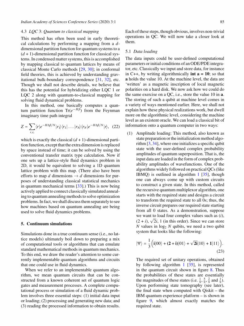
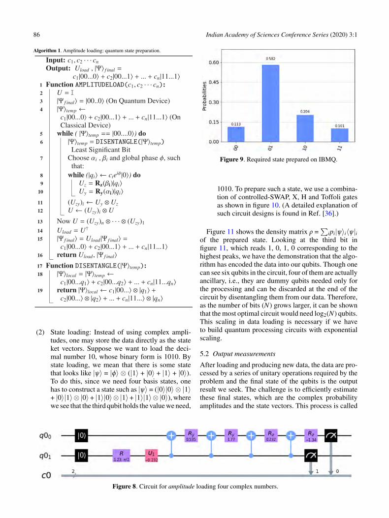
(1) Amplitude loading: This method, also known asstate preparation or the initialization method algo-rithm [3, 34], where one initializes a specific qubitstate with the user-defined complex probabilityamplitudes of quantum superposition. That is, theinput data are loaded in the form of complex prob-ability amplitudes of wavefunctions. One of thealgorithms widely followed on practical QCs (likeIBMQ) is outlined in algorithm 1 [35], thoughone can always come up with custom circuitsto construct a given state. In this method, calledthe recursive quantum multiplexor algorithm, onestarts with the required state and designs a circuitto transform the required state to all 0s; thus, theinverse circuit prepares our required state startingfrom all 0 states. As a demonstration, supposewe want to load four complex values such as (i),(2 + i),

√2i, 1 (in this order). Since we can store

N values in log2 N qubits, we need a two qubitsystem that looks like the following:

|Ψ〉 =13

(i|00〉 + (2 + i)|01〉 +

√2i|10〉 + 1|11〉

).

(23)

The required set of unitary operations, obtainedby following algorithm 1 [35], is representedin the quantum circuit shown in figure 8. Thusthe probabilities of these states are essentiallythe magnitudes of these states (i.e. 1

9 , 59 , 2

9 and 19 ).

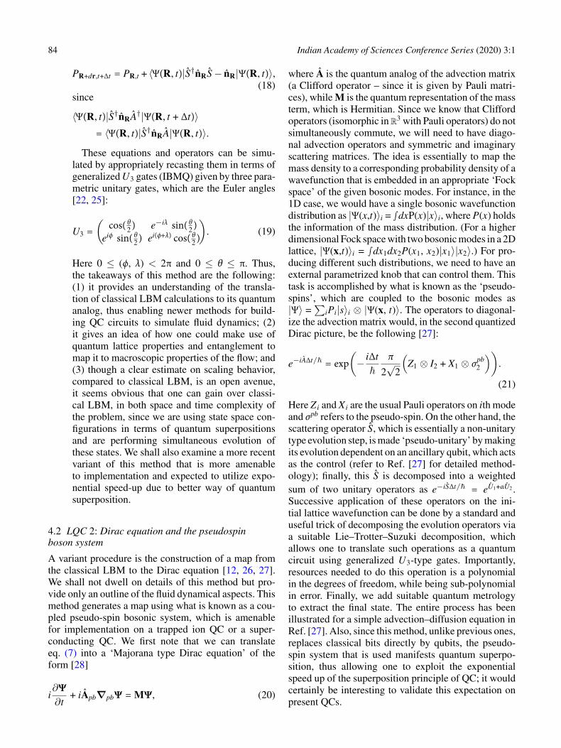
Upon performing state tomography (see later),the final state when computed with Qiskit – theIBM quantum experience platform – is shown infigure 9, which almost exactly matches therequired state.


Algorithm 1. Amplitude loading: quantum state preparation.

(2) State loading: Instead of using complex ampli-tudes, one may store the data directly as the stateket vectors. Suppose we want to load the deci-mal number 10, whose binary form is 1010. Bystate loading, we mean that there is some statethat looks like |ψ〉 = |ϕ〉 ⊗ (|1〉 + |0〉 + |1〉 + |0〉).To do this, since we need four basis states, onehas to construct a state such as |ψ〉 = (|0〉|0〉 ⊗ |1〉+ |0〉|1〉⊗ |0〉+ |1〉|0〉⊗ |1〉+ |1〉|1〉⊗ |0〉), wherewe see that the third qubit holds the value we need,

Figure 9. Required state prepared on IBMQ.

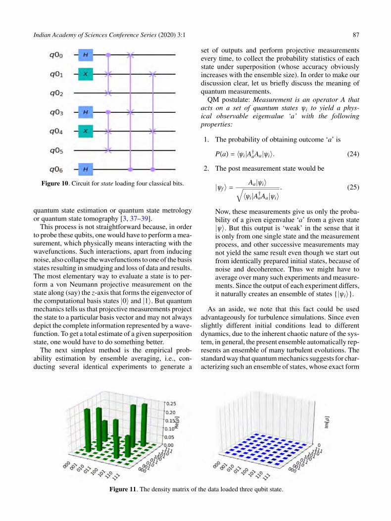
1010. To prepare such a state, we use a combina-tion of controlled-SWAP, X, H and Toffoli gatesas shown in figure 10. (A detailed explanation ofsuch circuit designs is found in Ref. [36].)

Figure 11 shows the density matrix ρ =∑

ipi|ψ〉i〈ψ|iof the prepared state. Looking at the third bit infigure 11, which reads 1, 0, 1, 0 corresponding to thehighest peaks, we have the demonstration that the algo-rithm has encoded the data into our qubits. Though onecan see six qubits in the circuit, four of them are actuallyancillary, i.e., they are dummy qubits needed only forthe processing and can be discarded at the end of thecircuit by disentangling them from our data. Therefore,as the number of bits (N) grows larger, it can be shownthat the most optimal circuit would need log2(N) qubits.This scaling in data loading is necessary if we haveto build quantum processing circuits with exponentialscaling.

5.2 Output measurements

After loading and producing new data, the data are pro-cessed by a series of unitary operations required by theproblem and the final state of the qubits is the outputresult we seek. The challenge is to efficiently estimatethese final states, which are the complex probabilityamplitudes and the state vectors. This process is called

Figure 8. Circuit for amplitude loading four complex numbers.


Figure 10. Circuit for state loading four classical bits.

quantum state estimation or quantum state metrologyor quantum state tomography [3, 37–39].

This process is not straightforward because, in orderto probe these qubits, one would have to perform a mea-surement, which physically means interacting with thewavefunctions. Such interactions, apart from inducingnoise, also collapse the wavefunctions to one of the basisstates resulting in smudging and loss of data and results.The most elementary way to evaluate a state is to per-form a von Neumann projective measurement on thestate along (say) the z-axis that forms the eigenvector ofthe computational basis states |0〉 and |1〉. But quantummechanics tells us that projective measurements projectthe state to a particular basis vector and may not alwaysdepict the complete information represented by a wave-function. To get a total estimate of a given superpositionstate, one would have to do something better.

The next simplest method is the empirical prob-ability estimation by ensemble averaging, i.e., con-ducting several identical experiments to generate a

set of outputs and perform projective measurementsevery time, to collect the probability statistics of eachstate under superposition (whose accuracy obviouslyincreases with the ensemble size). In order to make ourdiscussion clear, let us briefly discuss the meaning ofquantum measurements.

QM postulate: Measurement is an operator A thatacts on a set of quantum states ψi to yield a phys-ical observable eigenvalue ‘a’ with the followingproperties:

1. The probability of obtaining outcome ‘a’ is

P(a) = 〈ψi|A†aAa|ψi〉. (24)

2. The post measurement state would be

|ψf 〉 =Aa|ψi〉√〈ψi|A†aAa|ψi〉

. (25)

Now, these measurements give us only the proba-bility of a given eigenvalue ‘a’ from a given state|ψ〉. But this output is ‘weak’ in the sense that itis only from one single state and the measurementprocess, and other successive measurements maynot yield the same result even though we start outfrom identically prepared initial states, because ofnoise and decoherence. Thus we might have toaverage over many such experiments and measure-ments. Since the output of each experiment differs,it naturally creates an ensemble of states {|ψi〉}.

As an aside, we note that this fact could be usedadvantageously for turbulence simulations. Since evenslightly different initial conditions lead to differentdynamics, due to the inherent chaotic nature of the sys-tem, in general, the present ensemble automatically rep-resents an ensemble of many turbulent evolutions. Thestandard way that quantum mechanics suggests for char-acterizing such an ensemble of states, whose exact form

Figure 11. The density matrix of the data loaded three qubit state.


we have to probe, is to use the density operator formal-ism. If pα is the probability of obtaining a state {|ψα〉},the density operator is given by ρ =

∑αpα|ψα〉〈ψα|.

We may restate the previous measurement postulate interms of ρ as

1. The probability of obtaining outcome ‘a’ is

P(a) = Tr(A†aAaρ). (26)

2. Its post measurement state would be

ρf =AaρA†a√

Tr(A†aAaρ). (27)

The density operator has the property that Tr(ρ) = 1i.e., probabilities (non-negative eigenvalues) sum up tounity. Since we are only interested in obtaining thestatistics of each superposition state, we ask the ques-tion: What type of measurement procedure respectsthe positivity and completeness property of the den-sity operator as well as yield the probability amplitudesof the states in the ensemble? The answer is termedpositive operator valued measurements (POVM).The POVM elements constitute a set of operators{Pa

VM} ≡ {A†aAa} that are constrained to be positive,since 〈ψi|Pa

VM|ψi〉 = 〈ψi|A†aAa|ψi〉 = P(a) ≥ 0, andcomplete, i.e.,

∑a Pa

VM =∑

a A†aAa = I. In fact, as onecan easily observe, we can even get the measurementoperator corresponding to a given POVM element by√

PaVM = Aa.

We are generally not interested in the measurementitself but only in the statistics. Thus the POVM pro-vides a clean way of doing this without worrying aboutthe state itself. Another important advantage of posi-tive definiteness of these operators is that, for a givenset of non-orthogonal states, a POVM set of opera-tors {Pa

VM, PbVM and (Pc

VM = I − (PaVM + Pb

VM))} canbe used to compute their statistics or distinguish thestates. Thus, the output of sandwiching the operatorsbetween state vectors gives us the statistics. The opera-tors are designed to create a unique one-to-one mappingfrom the operator space to a particular output state. Soany positive output, resulting from the first two opera-tors in our set, points uniquely to a specific state, whilean output from the third operator implies that we can-not comment anything about the state. So, essentiallysuch a measurement process never lets us go wrong inidentifying states, but at the cost of being unable to com-ment about the output from one of its operators. Withthis machinery we are ready to look at quantum statetomography.

5.3 Quantum state tomography

Let us begin with a density matrix representing anunknown quantum state that needs to be profiled. Say we

have just one set of non-orthogonal qubit states. Exper-imentally it is impossible to construct the quantum statefrom just one copy of the states. But we can make severalPOVM measurements from multiple copies and com-pute the statistics. The set of operators {I/2, X/2, Y /2,Z/2} that form a set of orthonormal operators can beused to expand the density matrix as

ρ =12

(Tr(ρ)I + Tr(Xρ)X + Tr(Yρ)Y + Tr(Zρ)Z

). (28)

The expectation of these operators can be obtained byTr(Xρ). Now each of these expectation values can beestimated by repeated measurements. Once we have alarge sample size with good estimates of each of theseoperator outputs, we can reconstruct the density oper-ator of the unknown state. The standard deviation ofthe estimate is 1/

√N , where N is the ensemble size,

as one would expect for a Gaussian random variablein the large N limit. This in essence is the picture ofquantum state tomography. The same procedure can beextended to multiple qubit systems as well. This pro-cedure is usually achieved in practice by a few populartechniques [40] such as

1. Simple inversion2. Regression fits3. Maximum likelihood estimates4. Bayesian methods.

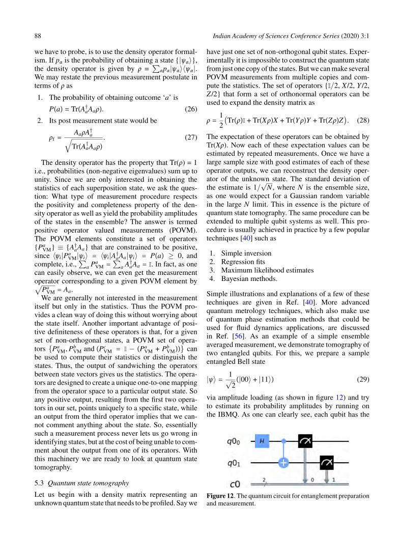
Simple illustrations and explanations of a few of thesetechniques are given in Ref. [40]. More advancedquantum metrology techniques, which also make useof quantum phase estimation methods that could beused for fluid dynamics applications, are discussedin Ref. [56]. As an example of a simple ensembleaveraged measurement, we demonstrate tomography oftwo entangled qubits. For this, we prepare a sampleentangled Bell state

|ψ〉 =1√2

(|00〉 + |11〉) (29)

via amplitude loading (as shown in figure 12) and tryto estimate its probability amplitudes by running onthe IBMQ. As one can clearly see, each qubit has the

Figure 12. The quantum circuit for entanglement preparationand measurement.


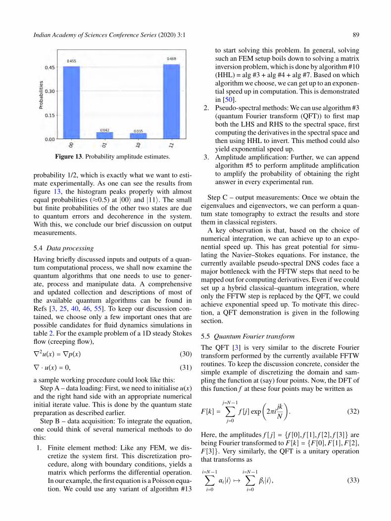
Figure 13. Probability amplitude estimates.

probability 1/2, which is exactly what we want to esti-mate experimentally. As one can see the results fromfigure 13, the histogram peaks properly with almostequal probabilities (≈0.5) at |00〉 and |11〉. The smallbut finite probabilities of the other two states are dueto quantum errors and decoherence in the system.With this, we conclude our brief discussion on outputmeasurements.

5.4 Data processing

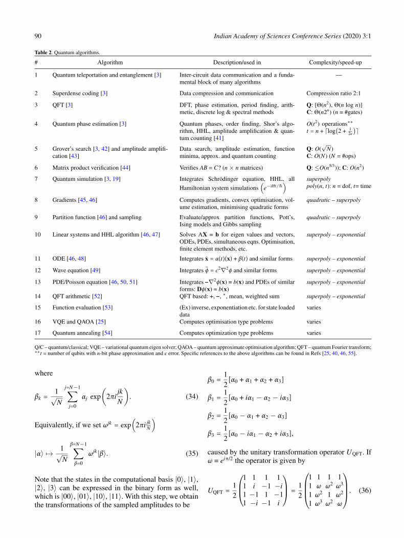
Having briefly discussed inputs and outputs of a quan-tum computational process, we shall now examine thequantum algorithms that one needs to use to gener-ate, process and manipulate data. A comprehensiveand updated collection and descriptions of most ofthe available quantum algorithms can be found inRefs [3, 25, 40, 46, 55]. To keep our discussion con-tained, we choose only a few important ones that arepossible candidates for fluid dynamics simulations intable 2. For the example problem of a 1D steady Stokesflow (creeping flow),

∇2u(x) = ∇p(x) (30)

∇ · u(x) = 0, (31)

a sample working procedure could look like this:Step A – data loading: First, we need to initialise u(x)

and the right hand side with an appropriate numericalinitial iterate value. This is done by the quantum statepreparation as described earlier.

Step B – data acquisition: To integrate the equation,one could think of several numerical methods to dothis:

1. Finite element method: Like any FEM, we dis-cretize the system first. This discretization pro-cedure, along with boundary conditions, yields amatrix which performs the differential operation.In our example, the first equation is a Poisson equa-tion. We could use any variant of algorithm #13

to start solving this problem. In general, solvingsuch an FEM setup boils down to solving a matrixinversion problem, which is done by algorithm #10(HHL) = alg #3 + alg #4 + alg #7. Based on whichalgorithm we choose, we can get up to an exponen-tial speed up in computation. This is demonstratedin [50].

2. Pseudo-spectral methods: We can use algorithm #3(quantum Fourier transform (QFT)) to first mapboth the LHS and RHS to the spectral space, firstcomputing the derivatives in the spectral space andthen using HHL to invert. This method could alsoyield exponential speed up.

3. Amplitude amplification: Further, we can appendalgorithm #5 to perform amplitude amplificationto amplify the probability of obtaining the rightanswer in every experimental run.

Step C – output measurements: Once we obtain theeigenvalues and eigenvectors, we can perform a quan-tum state tomography to extract the results and storethem in classical registers.

A key observation is that, based on the choice ofnumerical integration, we can achieve up to an expo-nential speed up. This has great potential for simu-lating the Navier–Stokes equations. For instance, thecurrently available pseudo-spectral DNS codes face amajor bottleneck with the FFTW steps that need to bemapped out for computing derivatives. Even if we couldset up a hybrid classical–quantum integration, whereonly the FFTW step is replaced by the QFT, we couldachieve exponential speed up. To motivate this direc-tion, a QFT demonstration is given in the followingsection.

5.5 Quantum Fourier transform

The QFT [3] is very similar to the discrete Fouriertransform performed by the currently available FFTWroutines. To keep the discussion concrete, consider thesimple example of discretizing the domain and sam-pling the function at (say) four points. Now, the DFT ofthis function f at these four points may be written as

F[k] =j=N−1∑

j=0

f [j] exp(

2πijkN

). (32)

Here, the amplitudes f [ j] = {f [0], f [1], f [2], f [3]} arebeing Fourier transformed to F[k] = {F[0], F[1], F[2],F[3]}. Very similarly, the QFT is a unitary operationthat transforms as

i=N−1∑i=0

αi|i〉 7→i=N−1∑

i=0

βi|i〉, (33)


Table 2. Quantum algorithms.

# Algorithm Description/used in Complexity/speed-up

1 Quantum teleportation and entanglement [3] Inter-circuit data communication and a funda-mental block of many algorithms

—

2 Superdense coding [3] Data compression and communication Compression ratio 2:1

3 QFT [3] DFT, phase estimation, period finding, arith-metic, discrete log & spectral methods

Q: [Θ(n2), Θ(n log n)]C: Θ(n2n) (n = #gates)

4 Quantum phase estimation [3] Quantum phases, order finding, Shor’s algo-rithm, HHL, amplitude amplification & quan-tum counting [41]

O(t2) operations∗∗

t = n + dlog(2 + 1

2ε

)e

5 Grover’s search [3, 42] and amplitude amplifi-cation [43]

Data search, amplitude estimation, functionminima, approx. and quantum counting

Q: O(√

N)C: O(N) (N = #ops)

6 Matrix product verification [44] Verifies AB = C? (n × n matrices) Q: ≤O(n5/3)); C: O(n2)

7 Quantum simulation [3, 19] Integrates Schrödinger equation, HHL, all

Hamiltonian system simulations(

e−iHt/~) superpoly

poly(n, t): n = dof, t= time

8 Gradients [45, 46] Computes gradients, convex optimisation, vol-ume estimation, minimising quadratic forms

quadratic – superpoly

9 Partition function [46] and sampling Evaluate/approx partition functions, Pott’s,Ising models and Gibbs sampling

quadratic – superpoly

10 Linear systems and HHL algorithm [46, 47] Solves AX = b for eigen values and vectors,ODEs, PDEs, simultaneous eqns. Optimisation,finite element methods, etc.

superpoly – exponential

11 ODE [46, 48] Integrates x = α(t)(x) + β(t) and similar forms superpoly – exponential

12 Wave equation [49] Integrates ϕ = c2∇2ϕ and similar forms superpoly – exponential

13 PDE/Poisson equation [46, 50, 51] Integrates �∇2ϕ(x) = b(x) and PDEs of similarforms: Dϕ(x) = b(x)

superpoly – exponential

14 QFT arithmetic [52] QFT based: +, �, ∗, mean, weighted sum superpoly – exponential

15 Function evaluation [53] (Ex) inverse, exponentiation etc. for state loadeddata

varies

16 VQE and QAOA [25] Computes optimisation type problems varies

17 Quantum annealing [54] Computes optimization type problems varies

Q/C – quantum/classical; VQE – variational quantum eigen solver; QAOA – quantum approximate optimisation algorithm; QFT – quantum Fourier transform;∗∗t = number of qubits with n-bit phase approximation and ε error. Specific references to the above algorithms can be found in Refs [25, 40, 46, 55].

where

βk =1√N

j=N−1∑j=0

αj exp(

2πijkN

). (34)

Equivalently, if we set ωjk = exp(

2πi jkN

)

|α〉 7→ 1√N

β=N−1∑β=0

ωjk|β〉. (35)

Note that the states in the computational basis |0〉, |1〉,|2〉, |3〉 can be expressed in the binary form as well,which is |00〉, |01〉, |10〉, |11〉. With this step, we obtainthe transformations of the sampled amplitudes to be

β0 =12

[α0 + α1 + α2 + α3]

β1 =12

[α0 + iα1 − α2 − iα3]

β2 =12

[α0 − α1 + α2 − α3]

β3 =12

[α0 − iα1 − α2 + iα3],

caused by the unitary transformation operator UQFT. Ifω = eiπ/2 the operator is given by

UQFT =12

1 1 1 11 i −1 −i1 −1 1 −11 −i −1 i

=12

1 1 1 11 ω ω2 ω3

1 ω2 1 ω2

1 ω3 ω2 ω

. (36)


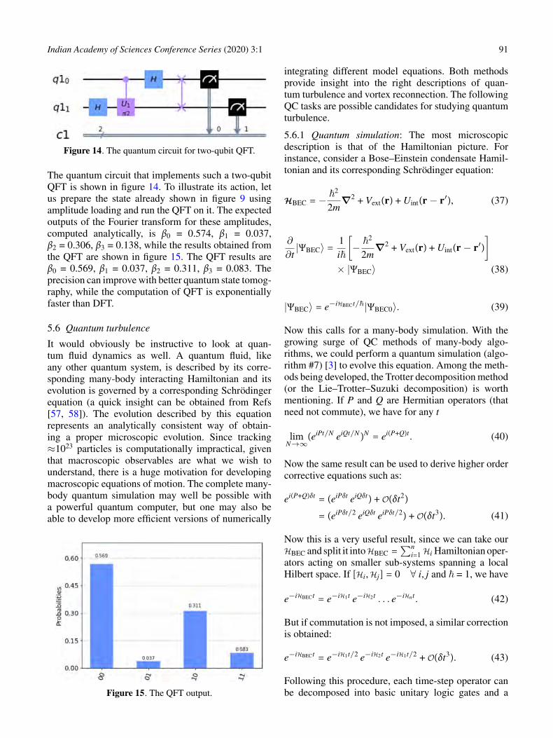
Figure 14. The quantum circuit for two-qubit QFT.

The quantum circuit that implements such a two-qubitQFT is shown in figure 14. To illustrate its action, letus prepare the state already shown in figure 9 usingamplitude loading and run the QFT on it. The expectedoutputs of the Fourier transform for these amplitudes,computed analytically, is β0 = 0.574, β1 = 0.037,β2 = 0.306, β3 = 0.138, while the results obtained fromthe QFT are shown in figure 15. The QFT results areβ0 = 0.569, β1 = 0.037, β2 = 0.311, β3 = 0.083. Theprecision can improve with better quantum state tomog-raphy, while the computation of QFT is exponentiallyfaster than DFT.

5.6 Quantum turbulence

It would obviously be instructive to look at quan-tum fluid dynamics as well. A quantum fluid, likeany other quantum system, is described by its corre-sponding many-body interacting Hamiltonian and itsevolution is governed by a corresponding Schrödingerequation (a quick insight can be obtained from Refs[57, 58]). The evolution described by this equationrepresents an analytically consistent way of obtain-ing a proper microscopic evolution. Since tracking≈1023 particles is computationally impractical, giventhat macroscopic observables are what we wish tounderstand, there is a huge motivation for developingmacroscopic equations of motion. The complete many-body quantum simulation may well be possible witha powerful quantum computer, but one may also beable to develop more efficient versions of numerically

Figure 15. The QFT output.

integrating different model equations. Both methodsprovide insight into the right descriptions of quan-tum turbulence and vortex reconnection. The followingQC tasks are possible candidates for studying quantumturbulence.

5.6.1 Quantum simulation: The most microscopicdescription is that of the Hamiltonian picture. Forinstance, consider a Bose–Einstein condensate Hamil-tonian and its corresponding Schrödinger equation:

HBEC = − ~2

2m∇2 + Vext(r) + Uint(r − r′), (37)

∂

∂t|ΨBEC〉 =

1i~

[− ~2

2m∇2 + Vext(r) + Uint(r − r′)

]× |ΨBEC〉 (38)

|ΨBEC〉 = e−iHBECt/~|ΨBEC0〉. (39)

Now this calls for a many-body simulation. With thegrowing surge of QC methods of many-body algo-rithms, we could perform a quantum simulation (algo-rithm #7) [3] to evolve this equation. Among the meth-ods being developed, the Trotter decomposition method(or the Lie–Trotter–Suzuki decomposition) is worthmentioning. If P and Q are Hermitian operators (thatneed not commute), we have for any t

limN→∞

(eiPt/N eiQt/N )N = ei(P+Q)t . (40)

Now the same result can be used to derive higher ordercorrective equations such as:

ei(P+Q)δt = (eiPδt eiQδt) + O(δt2)

= (eiPδt/2 eiQδt eiPδt/2) + O(δt3). (41)

Now this is a very useful result, since we can take ourHBEC and split it intoHBEC =

∑ni=1 Hi Hamiltonian oper-

ators acting on smaller sub-systems spanning a localHilbert space. If [Hi,Hj] = 0 ∀ i, j and ~ = 1, we have

e−iHBECt = e−iH1t e−iH2t . . . e−iHnt . (42)

But if commutation is not imposed, a similar correctionis obtained:

e−iHBECt = e−iH1t/2 e−iH2t e−iH1t/2 + O(δt3). (43)

Following this procedure, each time-step operator canbe decomposed into basic unitary logic gates and a


corresponding evolution circuit can be constructed.The following model equations would be amenable tonumerical integration using QC algorithms.

5.6.2 The two-fluid model: Simulating the Landau’sequations would be useful for those looking at quan-tum fluids at low velocities and with no quantum vor-tices, since this model works best for irrotational andincompressible flows. The idea would be to build onthe previously discussed algorithms for dealing withODEs and PDEs procedures to integrate the followingequations:

∂u1

∂t+ u1 · ∇u1 = −∇

(p1

ρ1

), (44)

∂u2

∂t+ u2 · ∇u2 = −∇

(p2

ρ2

)+νρ2∇2u2. (45)

Here the subscripts 1 and 2 correspond to superfluid andnormal fluid, respectively. Let us now look at methodsthat includes quantum vortices as well.

5.6.3 Gross–Pitaevskii model: Along with a few approx-imations and assumptions, we can use the standard trickof Madelung transformation to establish a relationshipbetween the BEC wavefunction and fluid macroscopicproperties such as density and velocity. This is theGross–Pitaevskii equation

∂

∂t|Ψcond〉 =

1i~

[− ~2

2m∇2 + Vext(r)

+ Uint|〈Ψcond|Ψcond〉|]|Ψcond〉. (46)

The built-in assumptions are (a) though the actualBEC wavefunction is a sum of the actual condensatewavefunction and the perturbative term, at T ∼ 0,we say ΨBEC ≈ Ψcond. (b) Length scales are of theorder of the vortex cores. (c) Only contact interac-tions are allowed U int = Uδ(r − r′). This model isthe nearest microscopic description, yet has many lim-itations. A detailed outlook could be obtained fromRefs [57, 58].

5.6.4 Vortex filament model: The next level would beto move to scales greater than the vortex core sizes.We visualise the fluid as an ensemble of arcs of quan-tum vortices and track these vortex arcs l, which is thevortex filament model. The evolution of these arcs isgiven by

dldt

= usa + uf , (47)

where usa is the self-advecting velocity of the vor-tex and uf is the mutual friction between the normalfluid arc surface. The computationally heavy step to bedone by the QC is the evaluation of the Biot–Savartintegral

ui =Γ

4π

∮(l− l′)|l− l′|3

× dl, (48)

to compute usa, Γ being the circulation of the vortexfilaments.

5.6.5 HVBK model: This model, obtained from aslight amendment of Landau’s equation, gives the bestdescription for the largest scales, much larger than thecore size. The additional terms are the mutual frictionforce fmf and the arc tension force fT. This modeltoo has limitations owing to its assumptions on thevortex arc orientations. The equations are (let us callF = fmf + fT):

∂u1

∂t+ u1 · ∇u1 = −∇

(p1

ρ1

)− F, (49)

∂u2

∂t+ u2 · ∇u2 = −∇

(p2

ρ2

)+νρ2∇2u2 +

ρ1

ρ2F. (50)

6. Variational solvers and quantum annealers

The last method to be outlined is based on variationaloptimization. Suppose we want to solve the conven-tional CFD problem of simulating a Stokes flow byusing a discretization solver such as Gauss–Seidel orJacobi. The problem reduces to solving for eigenvaluesof the form Ax = B using the HHL algorithm. It canalso be solved as an optimization problem. That is, wedefine a cost function such as the difference betweenthe LHS and RHS of the eigenvalue problem, and iter-ate and modify x so as to minimise the cost function to 0.Classical methods include algorithms such as gradientdescent, steepest descent, conjugate gradient method,etc. Such optimization procedures could be used for QCas well.

6.1 Variational quantum eigen (VQE) solver

The idea stems from the principle of quantum mechan-ics for solving the eigenvalue problems variationally. Itis usually done as a hybrid of quantum and classicalcomputing. So far, VQE has been applied for differ-ent condensed matter and quantum chemistry problems,but it can be extended to other problems as well. Ona hybrid machine, the steps are noted below. Detaileddescriptions can be found in Refs [25, 40, 59].


1. Consider a matrix P with one of its eigenvectors|ψp〉. Then we know that |ψp〉 is invariant in thesense of P|ψp〉 = p|ψp〉, where p is the correspond-ing eigenvalue. Let us regard P as a Hamiltonian,which is a positive definite Hermitian matrix, withpositive and real eigenvalues. Thus, the expecta-tion value of the Hamiltonian is 〈ψ|H|ψ〉 ≥ 0.The smallest eigenvalue pmin ≤ 〈ψ|H|ψ〉 corre-sponds to the ground-state energy of the system(≥0), which can be estimated by algorithm 2.

2. Thus while a quantum processing units (QPU)computes expectation values, the CPU runs anoptimisation algorithm; together they can be usedto estimate the eigenvalue and ground state config-urations.

6.2 Quantum approximate optimisationalgorithms (QAOA)

Generally, combinatorial optimization methods maynot be tractable with polynomial resources. Otherthan developing problem specific methods, approximatealgorithms such as QAOA can be handy. The goal isto take a discrete variable as an input, which could bestrings of binaries such as x = x1. . .xn, where xi ∈ {0, 1}defines a cost function E(x) that needs to be maxi-mized. The cost function is essentially a map fromE(x) : {0, 1}n 7→ R. The QAOA [25, 40, 60] thusforms the set of algorithms which does exactly this, andguarantees that the approximation ratio α satisfies

α =E(x)Emax

≥ αopt. (51)

Algorithm 2. Variational quantum eigenvalue solver.

6.3 Quantum annealing

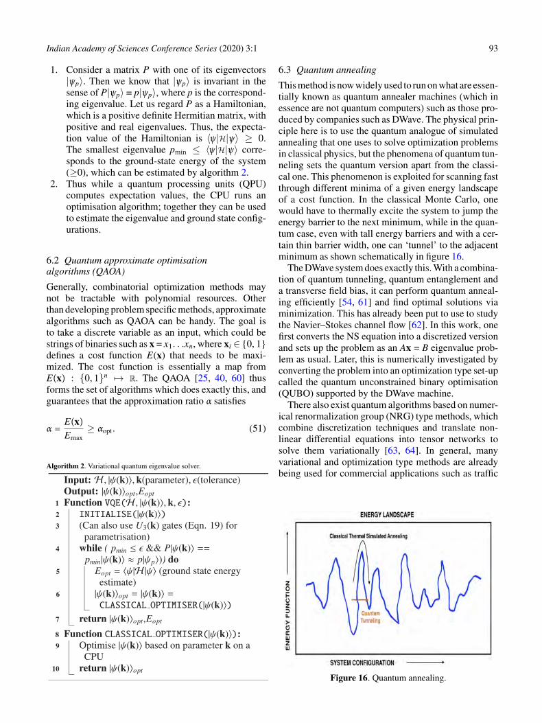
This method is now widely used to run on what are essen-tially known as quantum annealer machines (which inessence are not quantum computers) such as those pro-duced by companies such as DWave. The physical prin-ciple here is to use the quantum analogue of simulatedannealing that one uses to solve optimization problemsin classical physics, but the phenomena of quantum tun-neling sets the quantum version apart from the classi-cal one. This phenomenon is exploited for scanning fastthrough different minima of a given energy landscapeof a cost function. In the classical Monte Carlo, onewould have to thermally excite the system to jump theenergy barrier to the next minimum, while in the quan-tum case, even with tall energy barriers and with a cer-tain thin barrier width, one can ‘tunnel’ to the adjacentminimum as shown schematically in figure 16.

The DWave system does exactly this. With a combina-tion of quantum tunneling, quantum entanglement anda transverse field bias, it can perform quantum anneal-ing efficiently [54, 61] and find optimal solutions viaminimization. This has already been put to use to studythe Navier–Stokes channel flow [62]. In this work, onefirst converts the NS equation into a discretized versionand sets up the problem as an Ax = B eigenvalue prob-lem as usual. Later, this is numerically investigated byconverting the problem into an optimization type set-upcalled the quantum unconstrained binary optimisation(QUBO) supported by the DWave machine.

There also exist quantum algorithms based on numer-ical renormalization group (NRG) type methods, whichcombine discretization techniques and translate non-linear differential equations into tensor networks tosolve them variationally [63, 64]. In general, manyvariational and optimization type methods are alreadybeing used for commercial applications such as traffic

Figure 16. Quantum annealing.


flow management and finance management with verybig quantum annealers such as DWave which is offer-ing 5000 qubits. Though the complexity estimates ofthese methods vary and are not yet clearly estab-lished, they still offer a lucrative quantum protocolthat can solve optimization problems with a decentspeed-up.

7. Quantum programming and machines

Coming to the implementation and the actual execu-tion of these ideas and algorithms, what we need are(a) efficient quantum computer simulators to test thecorrectness of quantum algorithms and (b) real QCdevices to execute and assess the quantum advantageof practical QCs. There are now a large and growingnumber of efforts that have already built and are tryingto build, better quantum computers. Each of these QCsis being implemented using different quantum physicalrealizations and quantum materials that would be robustagainst external noise and decoherence, called QPU orquantum processors. Given a QPU, the process of pro-gramming a set of quantum algorithms and converting

them into forms understandable by a quantum machine,using instructions of suitable programming languages,is called quantum programming.

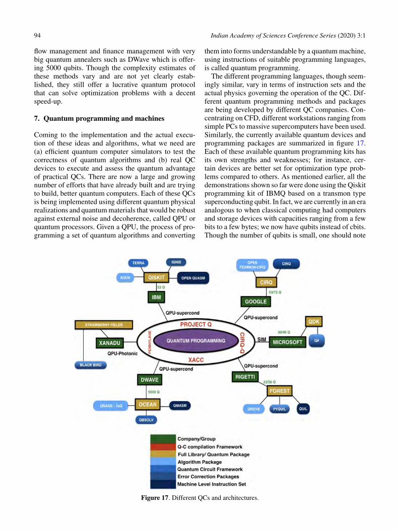
The different programming languages, though seem-ingly similar, vary in terms of instruction sets and theactual physics governing the operation of the QC. Dif-ferent quantum programming methods and packagesare being developed by different QC companies. Con-centrating on CFD, different workstations ranging fromsimple PCs to massive supercomputers have been used.Similarly, the currently available quantum devices andprogramming packages are summarized in figure 17.Each of these available quantum programming kits hasits own strengths and weaknesses; for instance, cer-tain devices are better set for optimization type prob-lems compared to others. As mentioned earlier, all thedemonstrations shown so far were done using the Qiskitprogramming kit of IBMQ based on a transmon typesuperconducting qubit. In fact, we are currently in an eraanalogous to when classical computing had computersand storage devices with capacities ranging from a fewbits to a few bytes; we now have qubits instead of cbits.Though the number of qubits is small, one should note

Figure 17. Different QCs and architectures.


that computing capacity can be exponentially largercompared to its classical counterparts.

Finally, let us consider the IBMQ 54-qubit machinefor some specific remarks.

1. QFT: In most DNS simulations, the FFT step ishighly time consuming. With 54 qubits, we canencode and compute the FFT of 254 ≈ 1016 com-plex numbers exponentially faster than the classi-cal version. This by itself, if implemented coher-ently, can greatly speed-up DNS calculations.

2. DNS grid sizes: With a 54-qubit machine we canstore and compute on

(a) 1D: ≤1016 meshes(b) 2D: ≤108 × 108 meshes(c) 3D: ≤105 × 105 × 105 meshes.

Here, each of these mesh sizes is far higher thanthe largest available DNS computations at present.

With these quantum algorithmic subroutines, at thisstage itself, exponential speed-ups are possible, andtheir robust implementation can ease the computationalchallenges facing DNS.

8. Conclusions

We have discussed and illustrated a selected collec-tion of quantum methods and tools for QCFD simu-lations. Most of these tools present at least a quadraticspeed-up, sometimes superpolynomial or exponential,compared to their classical counterparts. This in itselfis an incentive for the QCFD study. The existence ofcommercially available QCs such as IBMQ provides anadditional thrust to this entire effort. We wish to bringto the reader’s attention that quantum error correctionand decoherence reduction methods form a key fieldof study, the whole scope is to reduce noise-relatederrors and make QC codes more robust and accurate.For fluid dynamicists, the onset of QC provides a uniqueand exciting opportunity to study the subject in a com-pletely new way. Progress calls for familiarity withthis new paradigm of computing, building and puttingtogether newer and existing quantum algorithms forQCFD solvers. Since we are still in the early stage, itwould be wise to perform hybrid computations, wheresome functions are done on a QPU with the others ona CPU or GPU. As a concluding thought, this paper isintended to motivate the pursuit of new directions ofcomputational fluid mechanics that have the potentialof a huge impact.

Acknowledgements

The authors acknowledge the use of the IBM Q andIBM Q Experience platform for this work. The views

expressed are those of the authors and do not reflectthe official policy or position of IBM or the IBMQ team. The authors would like to thank Jörg Schu-macher, Dhawal Buaria and Kartik P. Iyer for insightfuldiscussions.

References

[1] R P Feynman, Int. J. Theor. Phys. 21, 467 (1999)[2] J Preskill, Quantum 2, 79 (2018)[3] M A Nielsen and I L Chuang, Quantum Computa-

tion and Quantum Information, 10th Anniversary edn(Cambridge University Press, Cambridge, UK, 2002)

[4] S A Orszag and G S Patterson Jr, Phys. Rev. Lett. 28, 76(1972)

[5] R S Rogallo, National aeronautics and space adminis-tration, 81315 (1981)

[6] S B Pope, Turbulent Flows (Cambridge UniversityPress, Cambridge, UK, 2001)

[7] P K Yeung, D A Donzis and K R Sreenivasan, Phys.Fluids 17, 081703 (2005)

[8] K P Iyer, J D Scheel, J Schumacher and K R Sreeni-vasan, Proc. Natl. Acad. Sci. 117, 7594 (2020)

[9] J Smagorinsky, B Galperin and S Orszag, Evolution ofPhysical Oceanography (Cambridge University Press,Cambridge, UK, 1993)

[10] C Meneveau and J Katz, Annu. Rev. Fluid Mech. 32, 1(2000)

[11] P A Davidson, Turbulence: An Introduction for Scien-tists and Engineers, 2nd edn (Oxford University Press,Oxford, UK, 2015)

[12] S Succi, R Benzi and F Higuera, Phys. D 47, 219 (1991)[13] S Succi, The Lattice Boltzmann Equation for Fluid

Dynamics and Beyond (Oxford University Press,Oxford, UK, 2001)

[14] D A Meyer, J. Stat. Phys. 85, 551 (1996)[15] D A Meyer, Philos. Trans. R. Soc., A 360, 395 (2002)[16] B M Boghosian and W Taylor IV, Int. J. Mod. Phys. C

8, 705 (1997)[17] B M Boghosian and W Taylor IV, Phys. Rev. E: Stat.

Phys., Plasmas, Fluids, Relat. Interdiscip. Top. 57, 54(1998)

[18] B M Boghosian and W Taylor IV, Phys. D 120, 30(1998)

[19] S Lloyd, Science 273, 1073 (1996)[20] D S Abrams and S Lloyd, Phys. Rev. Lett. 79, 2586

(1997)[21] J Yepez, Int. J. Mod. Phys. C 9, 1587 (1998)[22] J Yepez, Phys. Rev. E: Stat., Nonlinear, Soft Matter Phys.

63, 046702 (2001)[23] J Yepez, Int. J. Mod. Phys. C 12, 1285 (2001)[24] J Yepez, J. Stat. Phys. 107, 203 (2002)[25] IBM, IBMQ Qiskit Textbook, https:qiskit.org/textbook/

preface.html[26] R Benzi, S Succi and M Vergassola, Phys. Rep. 222,

145 (1992)


[27] A Mezzacapo, M Sanz, L Lamata, I L Egusquiza,S Succi and E Solano, Sci. Rep. 5, 13153 (2015)

[28] F Fillion-Gourdeau, H J Herrmann, M Mendoza, SPalpacelli and S Succi, Phys. Rev. Lett. 111, 160602(2013)

[29] S L Sondhi, S M Girvin, J P Carini and D Shahar, Rev.Mod. Phys. 69, 315 (1997)

[30] T H Hsieh, Student Rev. 1, 11 (2016)[31] O Aharony, S S Gubser, J Maldacena, H Ooguri and

Y Oz, Phys. Rep. 323, 183 (2000)[32] A M Polyakov, Contemp. Concepts Phys. 3, 1 (1987)[33] R D Somma, C D Batista and G Ortiz, Phys. Rev. Lett.

99, 030603 (2007)[34] M Plesch and ƒ Brukner, Phys. Rev. A: At., Mol., Opt.

Phys. 83, 032302 (2011)[35] V V Shende, S S Bullock and I L Markov, IEEE TCAD

25, 1000 (2006)[36] J A Cortese and T M Braje, arXiv preprint,

arXiv:1803.01958 (2018)[37] K Vogel and H Risken, Phys. Rev. A: At., Mol., Opt.

Phys. 40, 2847 (1989)[38] U Leonhardt, Measuring the Quantum State of Light,

volume 22 (Cambridge University Press, Cambridge,UK, 1997)

[39] W Nawrocki, Quantum Standards and Instrumentation(Springer, Heidelberg, 2015)

[40] P J Coles et al., arXiv preprint, arXiv:1804.03719(2018)

[41] G Brassard, P Hoyer, M Mosca and A Tapp, Interna-tional Colloquium on Automata, Languages, and Pro-gramming, volume 820 (Springer, Berlin, Heidelberg,1998)

[42] L K Grover, Phys. Rev. Lett. 79, 325 (1997)[43] G Brassard, P Hoyer, M Mosca and A Tapp, Contemp.

Math. 305, 53 (2002)[44] H Buhrman and R Spalek, Proc. 17th Annual ACM-

SIAM Symp. on Discrete Algorithm (Society for Indus-trial and Applied Mathematics, 2006)

[45] S P Jordan, Phys. Rev. Lett. 95, 050501 (2005)[46] S Jordan, Quantum algorithm zoo, https://quantum

algorithmzoo.org/[47] A W Harrow, A Hassidim and S Lloyd, Phys. Rev. Lett.

103, 150502 (2009)[48] D W Berry, J. Phys. A: Math. Theor. 47, 105301 (2014)[49] P C S Costa, S Jordan and A Ostrander, Phys. Rev. A

99, 012323 (2019)[50] Y Cao, A Papageorgiou, I Petras, J Traub and S Kais,

New J. Phys. 15, 013021 (2013)[51] J M Arrazola, T Kalajdzievski, C Weedbrook and

S Lloyd, Phys. Rev. A 100, 032306 (2019)[52] L Ruiz-Perez and J C Garcia-Escartin, Quantum Inf.

Process. 16, 152 (2017)[53] S Hadfield, arXiv preprint, arXiv:1805.03265 (2018)[54] DWave, https://docs.dwavesys.com/docs/latest/c_gs_2.

htmll.[55] A Montanaro, NPJ Quantum Inf. 2, 1 (2016)[56] G Xu, A J Daley, P Givi and R D Somma, AIAA J. 56,

687 (2018)[57] C F Barenghi, L Skrbek and K R Sreenivasan, Proc.

Natl. Acad. Sci. 111, 4647 (2014)[58] C F Barenghi, V S L’vov and P E Roche, Proc. Natl.

Acad. Sci. 111, 4683 (2014)[59] A Peruzzo et al., Nat. Commun. 5, 4213 (2014)[60] E Farhi, J Goldstone and S Gutmann, arXiv preprint,

arXiv:1411.4028 (2014)[61] D A Battaglia, G E Santoro and E Tosatti, Phys.

Rev. E: Stat., Nonlinear, Soft Matter Phys. 71, 066707(2005)

[62] N Ray, T Banerjee, B Nadiga and S Karra, arXivpreprint, arXiv:1904.09033 (2019)

[63] M Lubasch, P Moinier and D Jaksch, J. Comput. Phys.372, 587 (2018)

[64] M Lubasch, J Joo, P Moinier, M Kiffner and D Jaksch,Phys. Rev. A 101, 010301(R) (2020)

Quantum computation of ﬂuid dynamics

Documents

Transcript of Quantum computation of ﬂuid dynamics