HAL Id: hal-02948598https://hal-normandie-univ.archives-ouvertes.fr/hal-02948598v2

Preprint submitted on 29 Sep 2020

HAL is a multi-disciplinary open accessarchive for the deposit and dissemination of sci-entific research documents, whether they are pub-lished or not. The documents may come fromteaching and research institutions in France orabroad, or from public or private research centers.

L’archive ouverte pluridisciplinaire HAL, estdestinée au dépôt et à la diffusion de documentsscientifiques de niveau recherche, publiés ou non,émanant des établissements d’enseignement et derecherche français ou étrangers, des laboratoirespublics ou privés.

Quantum circuits of CNOT gatesMarc Bataille

To cite this version:

Marc Bataille. Quantum circuits of CNOT gates. 2020. hal-02948598v2

Quantum circuits of CNOT gates

Marc Bataillemarc.bataille1@univ-rouen.fr

LITIS laboratory, Universite Rouen-Normandie ∗

Abstract

We study in details the algebraic structure underlying quantum circuitsgenerated by CNOT gates. Our results allow us to propose polynomial heuristicsto reduce the number of gates used in a given CNOT gates circuit and we alsogive algorithms to optimize this type of circuits in some particular cases.Finally we show how to create some usefull entangled states using a CNOT

gates circuit acting on a fully factorized state.

∗685 Avenue de l’Universite, 76800 Saint-Etienne-du-Rouvray. France.

1

1 Introduction

The controlled Pauli-X gate, also called the CNOT gate, is a very common and usefullgate in quantum circuits. This gate involves two qubits i and j in a n-qubit system.One of the two qubits (say qubit i) is the target qubit whereas the other qubit playsthe role of control. When the control qubit j is in the state |1〉 then a Pauli-X gate(i.e. a NOT gate) is applied to the target qubit i which gets flipped. When qubit jis in the state |0〉 nothing happens to qubit i.Actually, CNOT gates are of crucial importance in the fields of quantum computa-tion and quantum information. Indeed, it appears that single qubit unitary gatestogether with CNOT gates constitute an universal set for quantum computation :any arbitrary unitary operation on a n-qubit system can be implemented using onlyCNOT gates and single qubit unitary gates (see [29, Section 4.5.2] for a completeproof of this important result). As a consequence, many multiple-qubit gates areimplemented in current experimental quantum machines using CNOT gates plus othersingle-qubit gates. In Figure 3 we give a few classical examples of such an implemen-tation : a SWAP gate can be simulated using 3 CNOT gates, a controlled Pauli-Z gatecan be implemented by means of 2 Hadamard single-qubit gates and one CNOT gate.These implementations are used for instance in the IBM superconducting transmondevice (www.ibm.com/quantum-computing/).

From this universality result it is possible to show that any unitary operation canbe approximated to arbitrary accuracy using CNOT gates together with Hadamard,Phase, and π/8 gates (see Figure 2 for a definition of these gates and [29, Section4.5.3] for a proof of this result). This discrete set of gates is often called the standardset of universal gates. Using a discrete set of gates brings a great advantage in termsof reliability because it is possible to apply these gates in an error-resistant waythrough the use of quantum error-correcting codes (again refer to [29, Chapter 10]for further information). Currently, important error rates in CNOT gates implementedon experimental quantum computers are one of the main causes of their unreliability(see [24, 35] and Table 1). So the ability to correct errors on quantum circuits is akey point for successfully building a functional and reliable quantum computer. Acomplementary approach to the Quantum Error-Correction is to improve reliabilityby minimizing the number of gates and particularly the number of two-qubit gatesused in a given circuit. Our work takes place in this context : we show that a preciseunderstanding of the algebraic structures underlying circuits of CNOT gates makes itpossible to reduce and, in some special cases, to minimize the number of gates inthese circuits.

In this paper we also study the emergence of entanglement in CNOT gates circuitsand we show that these circuits are a convenient tool for creating many types of en-tangled states. These particular states of a quantum system were first mentionnedby Einstein, Podolsky and Rosen in their famous EPR article of 1935 [9] and inQuantum Information Theory (QIT) they can be considered as a fundamental phys-ical resource (see e.g. [22]). Entangled states turn out to be essential in many areasof QIT such as quantum error correcting codes [13], quantum key distribution [10]or quantum secret sharing [6]. Spectacular applications such as super-dense coding

1

[3] or quantum teleportation [32, 11, 30] are based on the use of classical entangledstates. This significant role played by entanglement represents for us a good reasonto understand how CNOT gates circuits can be used to create entangled states.

The paper is structured as follows. Section 2 is mainly a background section wherewe recall some classical notions in order to guide non-specialist readers. In Section 3we investigate the algebraic structure of the group generated by CNOT gates. Section4 will be dedicated to the optimization problem of CNOT gates circuits in the generalcase while in Section 5 we deal with optimization in particular subgroups of thegroup generated by CNOT gates. Finally in Section 6 we study how to use CNOT gatescircuits to create certain usefull entangled states.

CNOTij 0 1 2 3 40 1.035× 10−2

1 1.035× 10−2 9.658× 10−3

2 9.658× 10−3 9.054× 10−3

3 9.054× 10−3 8.838× 10−3

4 8.838× 10−3

Hi 2.656× 10−4 3.675× 10−4 2.581× 10−4 3.572× 10−4 2.831× 10−4

Table 1: Error rates for CNOT gates acting on qubits i and j and for Hadamard gates acting on qubiti, where i, j ∈ 0, 1, 2, 3, 4. The data comes from ibmq rome 5-qubit quantum computer after acalibration on May 12, 2020 and is publicly avalaible at www.ibm.com/quantum-computing/.

2 Quantum circuits, CNOT and SWAP gates

We recall here some definitions and basic facts about quantum circuits and CNOT

gates. We also introduce some notations used in this paper and we add some devel-opments about SWAP gates circuits. For a comprehensive introduction to quantumcircuits the reader may refer to [29, Chapter 4] or, for a shorter but self-containedintroduction), to our last article [2].In QIT, a qubit is a quantum state that represents the basic information storageunit. This state is described by a ket vector in the Dirac notation |ψ〉 = a0 |0〉+a1 |1〉where a0 and a1 are complex numbers such that |a0|2 + |a1|2 = 1. The value of |ai|2represents the probability that measurement produces the value i. The states |0〉and |1〉 form a basis of the Hilbert space H ' C2 where a one qubit quantum systemevolves.Operations on qubits must preserve the norm and are therefore described by unitaryoperators. In quantum computation, these operations are represented by quantumgates and a quantum circuit is a conventional representation of the sequence ofquantum gates applied to the qubit register over time. In Figure 1 we recall thedefinition of the Pauli gates : notice that the states |0〉 and |1〉 are eigenvectors of thePauli-Z operator respectively associated to the eigenvalues 1 and -1, i.e. Z |0〉 = |0〉and Z |1〉 = − |1〉. Hence the computational standard basis (|0〉 , |1〉) is also calledthe Z-basis.

2

Pauli-X

[0 11 0

]X

Pauli-Y

[0 −ii 0

]Y

Pauli-Z

[1 00 −1

]Z

Figure 1: The Pauli gates

A quantum system of two qubits A and B (also called a two-qubit register) lives ina 4-dimensional Hilbert space HA ⊗HB and the computational basis of this spaceis : (|00〉 = |0〉A ⊗ |0〉B , |01〉 = |0〉A ⊗ |1〉B , |10〉 = |1〉A ⊗ |0〉B , |11〉 = |1〉A ⊗ |1〉B).If U is any unitary operator acting on one qubit, a controlled-U operator acts onthe Hilbert space HA ⊗HB as follows. One of the two qubits (say qubit A) is thecontrol qubit whereas the other qubit is the target qubit. If the control qubit A isin the state |1〉 then U is applied on the target qubit B and if qubit A is in thestate |0〉 nothing is done on qubit B. If U is the Pauli-X operator then CNOT isnothing more than the controlled-X operator (also denoted by c−X) with control onqubit A and target on qubit B. So the action of CNOT on the two-qubit register isdescribed by : CNOT |00〉 = |00〉 , CNOT |01〉 = |01〉 , CNOT |10〉 = |11〉 , CNOT |11〉 = |10〉(the corresponding matrix is given in Figure 2). Notice that the action of the CNOT

gate on the system can be sum up by the following simple formula :

∀x, y ∈ 0, 1, CNOT |xy〉 = |x, x⊕ y〉 (1)

where ⊕ denotes the XOR operator between two bits which is also the addition in F2.To emphasize that qubit A is the control and B is the target, CNOT is also denotedCNOTAB. So interchanging the roles played by A and B yields another operatordenoted by CNOTBA.

∀x, y ∈ 0, 1, CNOTBA |xy〉 = |x⊕ y, y〉 (2)

CNOT :A

BCNOTAB =

1 0 0 00 1 0 00 0 0 10 0 1 0

Phase : S S =

[1 00 i

]

Hadamard : H H = 1√2

[1 11 −1

]π/8 : T T =

[1 0

0 eiπ4

]Figure 2: The standard set of universal gates : names, circuit symbols and matrices.

Another useful and common two-qubit quantum gate is the SWAP operator whoseaction on a basis state vector |xy〉 is given by : SWAP |xy〉 = |yx〉. The interestingpoint is that a SWAP gate can be simulated using 3 CNOT gates :

SWAP = CNOTABCNOTBACNOTAB = CNOTBACNOTABCNOTBA (3)

3

SWAP :A

B∼ ∼ (5)

CNOTBA :A

B∼ H

H

H

H(6)

c− Z :A

B∼ H H ∼

H H(7)

Figure 3: Some classical equivalences of circuits involving CNOT gates.

This identity can be proved easily using equations (1) and (2).

The depth of a quantum circuit is the number of gates composing this circuit andwe say that two circuits are equivalent if their action on the basis state vectors isthe same in theory, i.e. the two circuits represents the same unitary operator. SoIdentity (3) is a proof of equivalence (5) in Figure 3. This equivalence can be usedto implement a SWAP gate from 3 CNOT gates on an actual quantum machine. Twoequivalent circuits generaly do not have the same depth. We use the word equivalentinstead of the word equal to emphasize the fact that, due to the errors rate on gatesin all current implementations (see Figure 1), two equivalent circuits acting on twoqubits registers in the same input state will probably not produce in practice thesame output state. This experimental fact is an important technical problem and agood motivation to work on quantum circuits optimization.Equivalence (6) in Figure 3 is usefull in practice because the CNOTBA gate may not benative in some implementations, so we need to simulate it : this can be done usingthe native gate CNOTAB plus 4 Hadamard gates. Finally another classical equivalenceof quantum circuits involves the CNOT gate with the controlled Pauli-Z gate (alsodenoted by c−Z) and the Hadamard gate (equivalence (7) in Figure 3). We alreadymentionned it in the introduction to emphasize the ubiquity of the CNOT gates inquantum circuits as well as the importance of the universality theorem. Using thedefinitions of the Pauli-Z gate (Figure 1) and of a controlled-U gate, it is easy tocheck that the action of the c− Z gate on a basis state vector is defined by

∀x, y ∈ 0, 1, c− Z |xy〉 = (−1)xy |xy〉 (4)

and that it is invariant by switching the control and the target qubits. Equivalence(7) can be proved using the definition of the Hadamard gate (Figure 1) and Relation(4).

On a system of n qubits, we label each qubit from 0 to n − 1 thus following theusual convention. For coherence we also number the lines and columns of a matrixof dimension n from 0 to n−1 and we consider that a permutation of the symmetric

4

group Sn is a bijection of 0, . . . , n − 1. The n-qubit system evolves over time inthe Hilbert space H0 ⊗ H1 ⊗ · · · ⊗ Hn−1 where Hi is the Hilbert space of qubit i.Hence the Hilbert space of an n-qubit system is isomorphic to C2n . In this space,a state vector of the standard computational basis is denoted by |b0b1 · · · bn−1〉 withbi ∈ 0, 1. A CNOT gate with target on qubit i and control on qubit j will be denotedXij. The reader will pay attention to the fact that our convention is the opposite ofthe one generaly used in the literature (and in the beginning of this section) whereCNOTij denotes a CNOT gate with control on qubit i and target on qubit j. The reasonfor this convention is explained in the proof of Theorem 4, Section 3. So, if i < j,the action of Xij and Xji on a basis state vector is given by :

Xij |b0 · · · bi · · · bj · · · bn−1〉 = |b0 · · · bi ⊕ bj · · · bj · · · bn−1〉 , (8)

Xji |b0 · · · bi · · · bj · · · bn−1〉 = |b0 · · · bi · · · bj ⊕ bi · · · bn−1〉 . (9)

Notice that the Xi,j gates are (represented by) matrices of size 2n × 2n in the or-thogonal group O2n(R) and that they are permutation matrices.

X02 :

q0

q1

q2

1 0 0 0 0 0 0 00 0 0 0 0 1 0 00 0 1 0 0 0 0 00 0 0 0 0 0 0 10 0 0 0 1 0 0 00 1 0 0 0 0 0 00 0 0 0 0 0 1 00 0 0 1 0 0 0 0

Figure 4: The gate X02 in a 3-qubit circuit and its matrix in the standard basis.

To represent a permutation of Sn, we use the 2-line notation as well as the cyclenotation and the n × n permutation matrix whose entry (i, j) is 1 if i = σ(j) and0 otherwise. As an example, if σ ∈ S6 is the permutation defined by σ(0) =4, σ(1) = 5, σ(2) = 0, σ(3) = 3, σ(4) = 2, σ(5) = 1 then the 2-line notation is

σ =

(0 1 2 3 4 54 5 0 3 2 1

), a cycle notation can be σ = (204)(15) = (51)(420) or

σ = (204)(15)(3) if we want to write the one-cycle and the permutation matrix is

Mσ =

0 0 1 0 0 00 0 0 0 0 10 0 0 0 1 00 0 0 1 0 01 0 0 0 0 00 1 0 0 0 0

. The cycle type of a permutation σ ∈ Sn is the tuple

λ = (n1, n2, . . . , np) of positive integers such that n1 > n2 > . . . > np, n =∑p

i=1 niand σ is the commutative product of cycles of length ni (including the cycles oflength 1). This kind of tuple is called a decreasing partition of n. For instanceσ = (204)(15)(3) = (204)(15) has cycle type λ = (3, 2, 1). Notice that the cycletype of the identity is λ = (1, . . . , 1). Two permutations have the same cycle type

5

iff they are in the same conjugacy class. For instance σ′ = (350)(24) has the same

cycle type as σ and σ′ = γσγ−1 where γ =

(0 1 2 3 4 55 2 3 1 0 4

).

A SWAP gate between qubit i and qubit j is denoted by S(ij) where (ij) is the cyclicnotation for the transposition that exchange i and j. Since the symmetric groupSn is generated by the transpositions, it is straightforward to prove that the groupgenerated by the S(ij) is isomorphic to the symmetric group : each SWAP gate S(ij) ina n-qubit circuit corresponds to the transposition (ij) in Sn. Notice that the cyclicnotation of a transposition (i.e. (ij) = (ji)) implies S(ij) = S(ji) which is coherentwith the symmetry of a SWAP gate. More generaly any circuit of SWAP gates mapsto a permutation σ (examples in Figure 5 and Figure 13). If we denote by Sσ theunitary operator corresponding to that circuit one has :

Sσ |b0b1 · · · bn−1〉 = |bσ−1(0)bσ−1(1) · · · bσ−1(n−1)〉 (10)

σ = (024)(13) Sσ = S(02)S(24)S(13)

q0

q1

q2

q3

q4

Figure 5: A 5-qubit quantum circuit of SWAP gates and the corresponding permutation

3 The group generated by the CNOT gates

We denote by cXn (n > 2) the group generated by the n(n−1) gates (i.e. matrices)Xij.

cXn := 〈Xij | 0 6 i, j < n, i 6= j〉 (11)

X12X10X31X03 :

q0

q1

q2

q3

Figure 6: A circuit of cX4 and the corresponding operator.

6

Proposition 1. The following identities are satisfied by the generators of cXn.

Involution : X2ij = I (12)

Braid relation : XijXjiXij = XjiXijXji = S(ij) (13)

Commutation : (XijXk`)2 = I where i 6= `, j 6= k (14)

Non-commutation : (XijXjk)2 = (XjkXij)

2 = Xik (15)

Proof. One checks each identity A = B by showing that the actions of gates A andB on a basis state vector |b0 · · · bn−1〉 are the same. Using identities 8 and 9, theresults follow from direct computation let to the readers.

q0

q1

q2

q3

∼ ∼

X03 = X02X23X02X23 = X23X02X23X02

Figure 7: Example of Identity (15) in a cX4 circuit.

Using the identities from Proposition 1, one gets easily the conjugacy relations incXn :

XijXjkXij = XjkXik and XijXkiXij = XkiXkj. (16)

Let us denote by Sn the group generated by the Sij,

Sn :=⟨S(ij) | 0 6 i, j < n

⟩(17)

As explained at the end of Section 2, Sn is isomorphic to the symmetric group Sn

and Identity (13) implies that Sn is a subgroup of cXn. The action of Sn on cXn byconjugation is given by the following proposition :

Proposition 2. For any permutation σ in Sn and any i 6= j, one has :

SσXijSσ−1 = Xσ(i)σ(j). (18)

Proof. Since the transpositions generate the symmetric group, it suffices to provethe result when σ is a transposition, i.e. Sσ = Xk`X`kXk` for some ` 6= k. Hence,the result comes straightforwardly from equalities (12), (13), (14) and (16).

We denote by SLn(K) the special linear group on a field K and by Tij(n) the matrixIn + nEij where n ∈ K \ 0, i 6= j and Eij is the matrix with 0 on all entriesbut the entry (i, j) which is equal to 1. Let (ek)06k<n be the canonical basis of thevector space Kn and (e∗k)06k<n its dual basis. Then the matrix Tij(n) representsin the canonical basis the automorphism tij(n) : u → u + ne∗j(u)ei of Kn which is

7

q0

q1

q2

q3

∼ ∼

X03 = S(02)X23S(02) = S(23)X02S(23)

Figure 8: Example of Identity (18) in a cX4 circuit.

a transvection fixing the hyperplane 〈ek | k 6= j〉 and directed by the line 〈ei〉. SoTij(n) is a transvection matrix and this is a well known fact in linear algebra thatthe transvection matrices generate SLn(K). A simple way to find a decompositionin transvection matrices of any matrix M in SLn(K) is to use the Gauss-Jordanalgorithm with M as input. This algorithm is generaly used to compute an inverseof a matrix but it also yields a decomposition of M as a product of transvections(see Figure 11 in Section 4 for an example).If K = F2 then n = 1 and the set Tij(n)|n ∈ K is reduced to the n(n − 1)transvection matrices Tij := In + Eij. Moreover, since any invertible matrix ofGLn(F2) has determinant 1, one has :

GLn(F2) = 〈Tij | 0 6 i, j < n, i 6= j〉 . (19)

We recall that the Gauss-Jordan algorithm is based on the following observation :

Proposition 3. Multiplying to the left (resp. the right) any F2-matrix M by atransvection matrix Tij is equivalent to add the jth line (resp. ith column) to the ithline (resp. j column) in M .

In particular, one has

Tij

b0...bi...bj...

bn−1

=

b0...

bi ⊕ bj...bj...

bn−1

. (20)

The notation |b0b1 · · · bn−1〉 used in QIT is a shorthand for the tensor product |b0〉⊗|b1〉 ⊗ · · · ⊗ |bn−1〉 and it is convenient to identify the binary label b0b1 · · · bn−1 withthe column vector u = [b0, b1, · · · , bn−1]T of Fn2 since the ⊕ (XOR) operation betweentwo bits corresponds to the addition in F2. So the computational basis of the Hilbertspace H0⊗H1⊗· · ·⊗Hn−1 is from now on denoted by (|u〉)u∈Fn2 and using Relation

(20) we can rewrite Relation (8) in a much cleaner way as

Xij |u〉 = |Tiju〉 . (21)

The above considerations lead quiet naturally to the following theorem :

8

Theorem 4. The group cXn generated by the CNOT gates acting on n qubits isisomorphic to GLn(F2). The morphism Φ sending each Xij to Tij is an explicitisomorphism.

Proof. The surjectivity of Φ is due to the fact that GLn(F2) is generated by thetransvections Tij. Furthermore, due to Relation (21), a preimage N by Φ of amatrix M in GLn(F2) must satisfy the relation N |u〉 = |Mu〉 for any basis vector|u〉 and there is only one matrix N satisfying this relation. So Φ is also injectiveand the result is proved.

Notice that the image by Φ of a SWAP matrix S(ij) is a transposition matrix P(ij) :=TijTjiTij = TjiTijTji in GLn(F2) and more generaly Φ(Sσ) is the permutation matrixPσ for any permutation σ in Sn. From now on we will denote by Mσ = PσMP−1σ

the conjugate of a matrix M in GLn(F2) by a permutation matrix Pσ. Using theisomorphism Φ, Relation (18) leads to

T σij = PσTijP−1σ = Tσ(i)σ(j). (22)

The order GLn(F2) is classicaly obtained by computing the number of different basisof Fn2 and Theorem 4 implies

Corollary 5.

|cXn| = 2n(n−1)

2

n∏i=1

(2i − 1). (23)

In his ”Lectures on Chevalley Group” [31, Chapter 6], Steinberg gives a presentationof the special linear group on a finite field K in dimension n > 3. The notation (a, b)stands here for the commutator of two elements a and b of a group (i.e. a−1b−1ab)which is usualy denoted by [a, b].

Theorem 6. (Steinberg)If n > 3 and K is a finite field, the symbols xij(t), (1 6 i, j 6 n, i 6= j, t ∈ K)subject to the relations :

(A) xij(t)xij(u) = xij(t+ u)

(B) (xij(t), xjk(u)) = xik(tu) if i, j, k are distinct, (xij(t), xk`(u)) = 1

if j 6= k, i 6= `

define the group SLn(K).

It is straightforward to adapt this presentation to the case K = F2 and we get so apresentation for the group cXn for any n > 3.

9

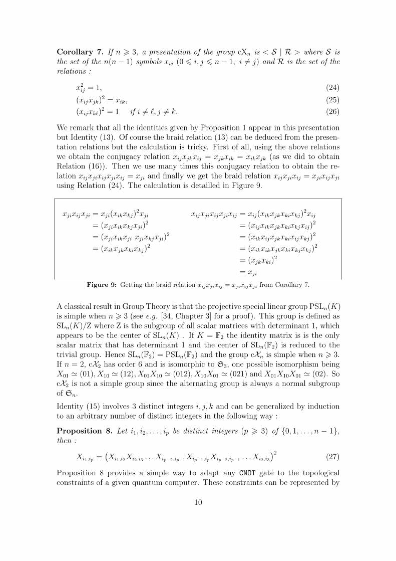
Corollary 7. If n > 3, a presentation of the group cXn is < S | R > where S isthe set of the n(n− 1) symbols xij (0 6 i, j 6 n− 1, i 6= j) and R is the set of therelations :

x2ij = 1, (24)

(xijxjk)2 = xik, (25)

(xijxk`)2 = 1 if i 6= `, j 6= k. (26)

We remark that all the identities given by Proposition 1 appear in this presentationbut Identity (13). Of course the braid relation (13) can be deduced from the presen-tation relations but the calculation is tricky. First of all, using the above relationswe obtain the conjugacy relation xijxjkxij = xjkxik = xikxjk (as we did to obtainRelation (16)). Then we use many times this conjugacy relation to obtain the re-lation xijxjixijxjixij = xji and finally we get the braid relation xijxjixij = xjixijxjiusing Relation (24). The calculation is detailled in Figure 9.

xjixijxji = xji(xikxkj)2xji

= (xjixikxkjxji)2

= (xjixikxji xjixkjxji)2

= (xikxjkxkixkj)2

xijxjixijxjixij = xij(xikxjkxkixkj)2xij

= (xijxikxjkxkixkjxij)2

= (xikxijxjkxkixijxkj)2

= (xikxikxjkxkixkjxkj)2

= (xjkxki)2

= xji

Figure 9: Getting the braid relation xijxjixij = xjixijxji from Corollary 7.

A classical result in Group Theory is that the projective special linear group PSLn(K)is simple when n > 3 (see e.g. [34, Chapter 3] for a proof). This group is defined asSLn(K)/Z where Z is the subgroup of all scalar matrices with determinant 1, whichappears to be the center of SLn(K) . If K = F2 the identity matrix is is the onlyscalar matrix that has determinant 1 and the center of SLn(F2) is reduced to thetrivial group. Hence SLn(F2) = PSLn(F2) and the group cXn is simple when n > 3.If n = 2, cX2 has order 6 and is isomorphic to S3, one possible isomorphism beingX01 ' (01), X10 ' (12), X01X10 ' (012), X10X01 ' (021) and X01X10X01 ' (02). SocX2 is not a simple group since the alternating group is always a normal subgroupof Sn.

Identity (15) involves 3 distinct integers i, j, k and can be generalized by inductionto an arbitrary number of distinct integers in the following way :

Proposition 8. Let i1, i2, . . . , ip be distinct integers (p > 3) of 0, 1, . . . , n − 1,then :

Xi1,ip =(Xi1,i2Xi2,i3 . . . Xip−2,ip−1Xip−1,ipXip−2,ip−1 . . . Xi2,i3

)2(27)

Proposition 8 provides a simple way to adapt any CNOT gate to the topologicalconstraints of a given quantum computer. These constraints can be represented by

10

a directed graph whose vertices are labelled by the qubits. There is an arrow fromqubit i to qubit j when these two qubits can interact to perform an Xij operationon the system. In a device with the complete graph topology, the full connectivityis achieved (see e.g. [24, 35]) and any Xij operation can be performed directly(i.e. without involving other two-qubit operations on other qubits than i and j).In contrast, the constraints in the LNN (Linear Nearest Neighbour) topology arestrong as direct interaction is allowed only on consecutive qubits, i.e. only Xi,i+1 orXi+1,i [36]. Of course there are also many intermediate graph configurations as inthe IBM superconducting transmon device (www.ibm.com/quantum-computing/).To implement a Xij gate when there is no arrow between i and j, the usual methodis to use SWAP gates together with allowed CNOT gates as we did in Figure 8. But,if SWAP gates are implemented on the device using 3 CNOT gates (circuit equivalence(5)), this implementation can be done in a more reliable fashion by using less gates :just find a shortest path (i1 = i, . . . , ip = j) between i and j in the undirected graph,then apply formula (27). Notice that it can be important to take into account theerror rate associated to each arrow (i, j) in the shortest path computation since itmay vary from one gate to another (see Figure 1). Case of (ik, ik+1) is not an arrow,use the classical equivalence 6 in Figure 3 to invert target and control. Of coursethis adds two single-qubit gates to the circuit but the impact on reliability is smallsince on current experimental quantum devices the fidelity of single qubit gates asthe Hadamard gate is much higher than any two-qubit gate fidelity (e.g. Figure 1again). In the example below, we implement a CNOT gate considering the topologyof the 15-qubit ibmq 16 melbourne device :

0 1 2 3 4 5 6

7891011121314

Choosen path to implement X4,7 : (4, 10, 9, 8, 7)

X4,7 = (X4,10X10,9X9,8X8,7X9,8X10,9)2

We end this section by remarking that GLp(F2) can be regarded as a subgroupof GLn(F2) if p < n. Indeed, let ϕ be the injective morphism from GLp(F2) into

GLn(F2) defined by ϕ(M) =

[M 00 In−p

], one has GLp(F2) ' ϕ(GLp(F2)), so we will

consider that GLp(F2) ⊂ GLn(F2) and no distinction will be made between matricesM and ϕ(M).

4 Optimization of CNOT gates circuits

A CNOT circuit is optimal if there is not another equivalent CNOT circuit with lessgates. In the same way a decomposition of a matrix M ∈ GLn(F2) in product oftransvections Ti,j is optimal if M cannot be written with less transvections. If thedepth of a circuit C ′ is less than the depth of an equivalent circuit C we say that C ′

11

is a reduction of C (or that C has been reduced to C ′) and if C ′ is optimal we saythat C ′ is an optimization of C (or that C has been optimized to C ′).For a better readability we denote from now on the transvection matrix Tij by [ij]and the permutation matrix Pσ by σ. As a consequence, (ij) denotes the transposi-tion which exchanges i and j as well as the transposition matrix P(ij). Notice that(ij) = (ji) but [ij] = [ji]T ([ij] is the transpose matrix of [ji]). With these notationsthe braid relation (13) becomes (ij) = (ji) = [ij][ji][ij] = [ji][ij][ji] and Identity(22) becomes σ[ij]σ−1 = [ij]σ = [σ(i)σ(j)]. In particular, (ij)[ij](ij) = [ij](ij) = [ji].

From Section 3, any CNOT circuit can be optimized using the following rewritingrules.

Proposition 9. Let 0 6 i, j, k, l 6 n− 1 be distinct integers :

[ij]2 = 1 (28)

[ij][jk][ik] = [ik][ij][jk] = [jk][ij] ; [ij][ki][kj] = [kj][ij][ki] = [ki][ij] (29)

[ij][jk][ij] = [jk][ik] = [ik][jk] ; [ij][ki][ij] = [ki][kj] = [kj][ki] (30)

[ij][kl] = [kl][ij] ; [ij][ik] = [ik][ij] ; [ij][kj] = [kj][ij] (31)

σ[ij] = [ij]σσ = [σ(i)σ(j)]σ ; [ij]σ = σ[ij]σ−1

= σ[σ−1(i)σ−1(j)] (32)

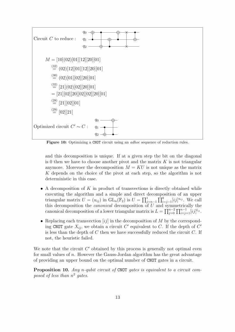
In practice one tries to find an ad hoc sequence of the above rules to reduce or to opti-mize a given circuit (see Figure 10 for an example) but the computation can be trickyeven with a few qubits. So it is difficult to build a general reduction/optimizationalgorithm from Proposition 9.

To optimize a CNOT circuit of a few qubits we use a C ANSI program that buildsthe Cayley Graph of the group GLn(F2) by Breadth-first search and then find in thegraph the group element corresponding to that circuit. This program optimizes in afew seconds any CNOT circuit up to 5 qubits and the source code can be downloaded athttps://github.com/marcbataille/cnot-circuits. In the rest of this article werefer to it as ”the computer optimization program”. However, due to the exponentialgrowth of the group order (for instance Card(cX6) = 20 158 709 760), the computermethod fails from 6 qubits with a basic PC. In this context we remark that theGauss Jordan algorithm mentionned in Section 3 can be used as a heuristic methodto reduce a given CNOT gates circuit (see Figure 11 for a detailled example). It worksas follows.

• Each Xij gate of a given circuit C corresponds to a transvection matrix [ij].Multiplying these transvection matrices yields a matrix M in GLn(F2) thatwe call the matrix of the circuit in dimension n.

• The Gauss-Jordan algorithm applied to the matrix M gives a decompositionof M under the form M = KU where U is an upper triangular matrix and K isa matrix that is a lower triangular matrix if and only if the element of F2 thatappears on the diagonal at each step of the algorithm is 1, so we can chooseit as pivot. In this case the matrix M as a LU (Lower Upper) decomposition

12

Circuit C to reduce :

q0

q1

q2

M = [10](02)[01][12][20][01]

(32)= (02)[12][01][12][20][01]

(30)= (02)[01][02][20][01]

(32)= [21](02)[02][20][01]

= [21][02][20][02][02][20][01]

(28)= [21][02][01]

(29)= [02][21]

Optimized circuit C ′ ∼ C :

q0

q1

q2

Figure 10: Optimizing a CNOT circuit using an adhoc sequence of reduction rules.

and this decomposition is unique. If at a given step the bit on the diagonalis 0 then we have to choose another pivot and the matrix K is not triangularanymore. Morevoer the decomposition M = KU is not unique as the matrixK depends on the choice of the pivot at each step, so the algorithm is notdeterministic in this case.

• A decomposition of K in product of transvections is directly obtained whileexecuting the algorithm and a simple and direct decomposition of an uppertriangular matrix U = (uij) in GLn(F2) is U =

∏1j=n−1

∏0i=j−1[ij]

uij . We callthis decomposition the canonical decomposition of U and symmetrically thecanonical decomposition of a lower triangular matrix is L =

∏n−2j=0

∏n−1i=j+1[ij]

lij .

• Replacing each transvection [ij] in the decomposition of M by the correspond-ing CNOT gate Xij, we obtain a circuit C ′ equivalent to C. If the depth of C ′

is less than the depth of C then we have successfully reduced the circuit C. Ifnot, the heuristic failed.

We note that the circuit C ′ obtained by this process is generally not optimal evenfor small values of n. However the Gauss-Jordan algorithm has the great advantageof providing an upper bound on the optimal number of CNOT gates in a circuit.

Proposition 10. Any n-qubit circuit of CNOT gates is equivalent to a circuit com-posed of less than n2 gates.

13

Proof. We apply the Gauss-Jordan elimination algorithm to get a decompositionof M ∈ GLn(F2) in transvections. The first part of the algorithm consists in mul-tiplying M to the left by a sequence of transvections in order to obtain an uppertriangular matrix U . For k = 0, 1, . . . , n − 1, we consider the column k and theentry of the matrix on the diagonal. If this entry is 1 we choose it as a pivot butif it is 0 we first need to put a 1 on the diagonal. This can be done by swapingrow k with a row ` whose entry (`, k) is 1. However, this will cost 3 transvectionsand it is more economical to add row ` to row k, i.e. multiplying to the left by[k, `]. The number of left multiplications by transvections necessary to have a pivotequal to 1 on the diagonal at each step is bounded by n − 1 and the number ofleft multiplications necessary to eliminate the 1’s below the pivot is bounded byn − 1 + · · · + 1 = n(n−1)

2. Hence the number of transvections that appears in the

first part of the algorithm is bounded by n(n+1)2− 1. In the second part of the

algorithm we just write the canonical decomposition of U which contains at mostn − 1 + n − 2 + · · · 1 = n(n−1)

2transvections. Finally we see that the number of

transvections in the resulting decomposition of M is at most n2 − 1.

INPUT : C =

q0

q1

q2

q3

M = [02][30][21][23][32][20][23][30][20][03][12][01]

M =

0 1 1 10 1 1 01 0 1 01 1 1 1

; [03]M =

1 0 0 00 1 1 01 0 1 01 1 1 1

; [31][20][30][03]M =

1 0 0 00 1 1 00 0 1 00 0 0 1

K = [03][30][20][31] ; U = [12] ; M = KU = [03][30][20][31][12]

OUTPUT : C ′ =

q0

q1

q2

q3

Figure 11: The Gauss-Jordan algorithm applied to a CNOT gates circuit.

The canonical decomposition of an upper or lower triangular matrix is generally notoptimal, so we propose in what follows another algorithm to decompose a triangularmatrix in transvections. Applying this algorithm to the matrix U when the decom-position of M is KU or to both matrices L and U when the decomposition of Mis LU can often improve the decomposition given by the Gauss-Jordan heuristic,especially when the triangular matrix has a high density of 1’s (See Figure 12 for anexample). We describe below this algorithm for an upper triangular matrix (UTDalgorithm) but it can be easily adapted to the case of a lower triangular matrix(LTD algorithm). We denote by |Li| is the number of 1’s in line i of a matrix.

14

Algorithm 11. Upper Triangular Decomposition (UTD algorithm)INPUT : An upper triangular matrix U in GLn(F2).OUTPUT : A sequence S = (t0, t1, . . . , tp−1) of transvections such that U =

∏p−1j=0 tj.

1 S = (); j = 0;2 while U 6= I :3 for i = 0 to n− 2 :4 if |Li| > 1 :5 Let Ei = k | i < k 6 n− 1 and |Li ⊕ Lk| < |Li|;6 if Ei 6= ∅ :7 Choose the smallest k ∈ Ei such that |Li ⊕ Lk| is minimal;8 U = [ik]U ;9 tj = [ik] ; j = j + 1;10 return S;

The algorithm ends because for each loop (for i = 0 to n − 2) the number of1’s in the matrix decreases of at least one. Indeed, there is always at least onecouple (i, k) choosen during this loop, namely : i = maxj | |Lj| > 1 and k =maxj | Uij 6= 0. Furthermore, we notice that the number of transvections in thedecomposition S is always less than or equal to the number of transvections in thecanonical decomposition of the matrix U since each transvection in the canonicaldecomposition of U contributes to a decrease of exactly one in the initial number of1’s in the matrix U whereas each transvection in S contributes to a decrease of atleast one in this initial number of 1’s.

Again, the decomposition obtained by applying the Gauss-Jordan algorithm followedby the UTD or LTD algorithm is generally not optimal. In fact we conjecture thefollowing result.

Conjecture 12. Any n-qubit circuit of CNOT gates is equivalent to a circuit composedof at most 3(n− 1) gates. The upper bound of 3(n− 1) gates is reached only in thespecial case of SWAP gates circuits Sσ where σ is a cycle of length n in Sn.

We checked this conjecture up to 5 qubits thanks to a C ANSI program (see theresults summarized in Table 2). The source code of the program can be downloadedat https://github.com/marcbataille/cnot-circuits.

5 Optimization in subgroups of cXnIn this section we describe the structure of some particular subgroups of cXn 'GLn(F2) and we propose algorithms to optimize CNOT gates circuits of these sub-groups. Starting from an input circuit C, we first compute the matrix M of thecircuit in dimension n. In some specific cases the matrix M has a particular shapeso we can propose an optimal decomposition in transvections for M and output anoptimization C ′ of the circuit C. We describe 3 subgroups corresponding to 3 typesof matrices with the objective of building step by step a kind of atlas of CNOT gatescircuits with specific optimization algorithms.

15

optimal length n = 2 n=3 n = 4 n = 5

l = 0 1 1 1 1l = 1 2 6 12 20l = 2 2 24 96 260l = 3 1 51 542 2 570l = 4 60 2 058 19 680l = 5 24 5 316 117 860l = 6 2 7 530 540 470l = 7 4 058 1 769 710l = 8 541 3 571 175l = 9 6 3 225 310l = 10 736 540l = 11 15 740l = 12 24

Order of cXn 6 168 20 160 9 999 360

Table 2: Number of elements of cXn having an optimal decomposition of length l. The numbersin bold correspond to the (n− 1)! cyclic permutations of length n.

5.1 Permutation matrices

The first case considered is when the matrix M ∈ GLn(F2) of the circuit is a permu-tation matrix Pσ. In this case the circuit is equivalent to a SWAP gates circuit andwe work in Sn, the subgroup of cXn generated by the S(ij) gates which is isomorphicto Sn (see example in Figure 13).

Proposition 13. Any permutation matrix Pσ can be decomposed as a product of3(n− p) transvections where p is the number of cycles of the permutation σ.

Proof. Let λ = (n1, . . . , np) be the cycle type of σ. Any cycle of length ni can bedecomposed in the product of ni − 1 transpositions and each transposition can bedecomposed in a product of 3 transvections, so the total number of transvectionsused in the decomposition of Pσ is 3

∑pi=1(ni − 1) = 3(n− p).

The following conjecture has been checked up to 5 qubits using the computer opti-mization program.

Conjecture 14. The decomposition in transvections of a permutation matrix Pσgiven by Proposition 13 is optimal.

5.2 Block diagonal matrices

In the second case, we consider that the matrix M of the circuit in dimension n is ablock diagonal matrix or the conjugate of a diagonal block matrix by a permutationmatrix. Let (n1, . . . , np) be a tuple of p positive integers such that

∑pi=1 ni = n and

16

INPUT : C =

q0

q1

q2

q3

q4

(13 CNOT)

M = [21][32][23][41][20][40][01][31][21][42][43][12][34]

M =

1 1 1 0 00 1 1 0 01 0 1 1 11 0 1 0 01 0 1 1 0

=

1 0 0 0 00 1 0 0 01 1 1 0 01 1 1 1 01 1 1 0 1

︸ ︷︷ ︸

L

1 1 1 0 00 1 1 0 00 0 1 1 10 0 0 1 10 0 0 0 1

︸ ︷︷ ︸

U

Canonical decomposition of L : L = [20][30][40][21][31][41][32][42]Canonical decomposition of U : U = [24][34][23][02][12][01]LTD algorithm −→ L = [42][32][21][20]UTD algorithm −→ U = [01][23][34][12]Hence : M = [42][32][21][20][01][23][34][12]

OUTPUT : C ′ =

q0

q1

q2

q3

q4

(8 CNOT)

Figure 12: The UTD/LTD algorithms applied to a LU circuit of CNOT gates

consider the matrix MS =

A1 0 . . . 0

0 A2. . .

......

. . . . . . 00 . . . 0 Ap

where S = (A1, . . . , Ap) is a tuple of

matrices Ai in GLni(F2). Here MS is a block diagonal matrix and we shall see rightafter the case of the conjugate of a block diagonal matrix by a permutation matrix.Clearly MS | S ∈ GLn1(F2)× · · · × GLnp(F2) is a group isomorphic to the directgroup product GLn1(F2)× · · · ×GLnp(F2) since

MS =

A1 0 . . . 0

0 In2

. . ....

.... . . . . . 0

0 . . . 0 Inp

× · · · ×In1 0 . . . 0

0. . . . . .

......

. . . Inp−1 00 . . . 0 Ap

where Iα is the identity

matrix in dimension α. This equality can be written as MS =∏p

i=1Mi where

17

q0

q1

q2

q3

C1 C2∼

q0

q1

q2

q3

C1 C2

M = Pσ =

0 1 0 00 0 1 00 0 0 11 0 0 0

; σ = (3210) = (23)(12)(01)

Figure 13: A cyclic permutation of the qubits between two circuits C1 and C2

Mi =

INi−10 0

0 Ai 00 0 In−Ni

and Ni =∑i

k=1 nk. We recall that the conjugation Mσ =

PσMP−1σ of a square matrix M by a permutation matrix Pσ has the following effecton M : if we denote by Li (resp. L′i) and Ci (resp. C ′i) the lines and columnsof matrix M (resp. Mσ) then L′i = Lσ−1(i) and C ′i = Cσ−1(i), hence if M = (mij)and M ′ = (m′ij) then m′ij = mσ−1(i)σ−1(j). So, if we consider now a tuple of ppermutations (σ1, . . . , σp) verifying the conditions σi(n1+n2+· · ·+ni−1) = 0, σi(n1+n2 + · · · + ni−1 + 1) = 1, . . . , σi(n1 + n2 + · · · + ni−1 + ni − 1) = ni − 1 then

MS =∏p

i=1 (Mσii )σ

−1i =

∏pi=1 (M ′

i)σ−1i where M ′

i =

[Ai 00 In−ni

]' Ai. Moreover,

for Relation (22), the number of transvections in an optimal decomposition of anymatrix M in GLn(F2) is the same as the number of transvections in an optimaldecomposition of Mσ for any permutation σ. As a consequence, the product of theconjugates by σ−1i of any optimal decomposition of the matrix Ai yields an optimaldecomposition of the matrix MS (see Figure 14 for an example).

The generalization of the previous situation to the case of a matrix M = MσS where

MS is a block diagonal matrix and σ a permutation matrix is straightforward. In-deed, if we have an optimal decomposition of MS in transvections, then we deducean optimal decomposition for Mσ

S by conjugating by σ each transvection in the de-composition of MS. This is due to the fact that the number of transvections in anoptimal decomposition of any matrix M in GLn(F2) is the same as the number oftransvections in an optimal decomposition of Mσ (see Relation (22)). In fact theproblem we adress here is rather the following : how can we efficiently recognize thatthe matrix M is of type M = Mσ

S ? To do that we interpret the matrix M of thecircuit in dimension n as the adjacency matrix of the directed graph G(M) whose setof vertices is V = 0, 1, . . . , n− 1 and whose set of edges is E = (i, j) | mij = 1.We call G(M) the graph of the circuit. The graph (G(M))σ defined by the set ofvertices σ(V ) = V and by the set of edges Eσ

n = (σ(i), σ(j)) | mij = 1 is isomor-phic to G(M). Besides, Eσ

n = (i, j) | mσ−1(i)σ−1(j) = 1 and Mσ =(mσ−1(i)σ−1(j)

),

so (G(M))σ = G(Mσ). The graph G(MS) is a disconnected graph whose p con-nected components are V1 = 0, . . . , n1 − 1, V2 = n1, . . . , n1 + n2 − 1, . . . , Vp =

18

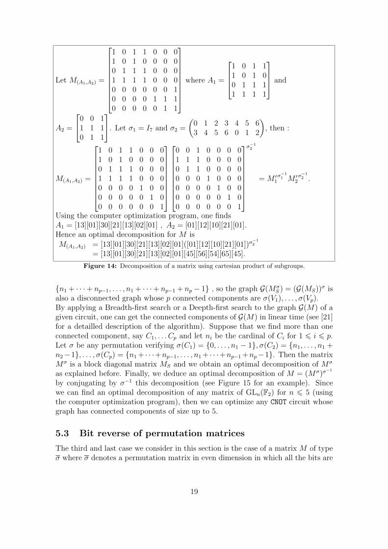
Let M(A1,A2) =

1 0 1 1 0 0 01 0 1 0 0 0 00 1 1 1 0 0 01 1 1 1 0 0 00 0 0 0 0 0 10 0 0 0 1 1 10 0 0 0 0 1 1

where A1 =

1 0 1 11 0 1 00 1 1 11 1 1 1

and

A2 =

0 0 11 1 10 1 1

. Let σ1 = I7 and σ2 =

(0 1 2 3 4 5 63 4 5 6 0 1 2

), then :

M(A1,A2) =

1 0 1 1 0 0 01 0 1 0 0 0 00 1 1 1 0 0 01 1 1 1 0 0 00 0 0 0 1 0 00 0 0 0 0 1 00 0 0 0 0 0 1

0 0 1 0 0 0 01 1 1 0 0 0 00 1 1 0 0 0 00 0 0 1 0 0 00 0 0 0 1 0 00 0 0 0 0 1 00 0 0 0 0 0 1

σ−12

= M ′1σ−11 M ′

2σ−12 .

Using the computer optimization program, one findsA1 = [13][01][30][21][13][02][01] , A2 = [01][12][10][21][01].Hence an optimal decomposition for M is

M(A1,A2) = [13][01][30][21][13][02][01]([01][12][10][21][01])σ−12

= [13][01][30][21][13][02][01][45][56][54][65][45].

Figure 14: Decomposition of a matrix using cartesian product of subgroups.

n1 + · · ·+ np−1, . . . , n1 + · · ·+ np−1 + np − 1 , so the graph G(MσS ) = (G(MS))σ is

also a disconnected graph whose p connected components are σ(V1), . . . , σ(Vp).By applying a Breadth-first search or a Deepth-first search to the graph G(M) of agiven circuit, one can get the connected components of G(M) in linear time (see [21]for a detailled description of the algorithm). Suppose that we find more than oneconnected component, say C1, . . . Cp and let ni be the cardinal of Ci for 1 6 i 6 p.Let σ be any permutation verifying σ(C1) = 0, . . . , n1 − 1, σ(C2) = n1, . . . , n1 +n2−1, . . . , σ(Cp) = n1 + · · ·+np−1, . . . , n1 + · · ·+np−1 +np−1. Then the matrixMσ is a block diagonal matrix MS and we obtain an optimal decomposition of Mσ

as explained before. Finally, we deduce an optimal decomposition of M = (Mσ)σ−1

by conjugating by σ−1 this decomposition (see Figure 15 for an example). Sincewe can find an optimal decomposition of any matrix of GLn(F2) for n 6 5 (usingthe computer optimization program), then we can optimize any CNOT circuit whosegraph has connected components of size up to 5.

5.3 Bit reverse of permutation matrices

The third and last case we consider in this section is the case of a matrix M of typeσ where σ denotes a permutation matrix in even dimension in which all the bits are

19

INPUT : C =

q0

q1

q2

q3

q4

q5

q6

(14 CNOT)

M =

1 0 0 1 0 1 10 1 1 0 1 0 00 0 0 0 1 0 00 0 0 0 0 1 10 1 0 0 1 0 01 0 0 0 0 1 11 0 0 1 0 0 1

C1 = 0, 3, 5, 6, C2 = 1, 2, 4

σ =

(0 1 2 3 4 5 63 5 4 1 6 0 2

)σ−1 =

(0 1 2 3 4 5 65 3 6 0 2 1 4

)

Mσ =

1 0 1 1 0 0 01 0 1 0 0 0 00 1 1 1 0 0 01 1 1 1 0 0 00 0 0 0 0 0 10 0 0 0 1 1 10 0 0 0 0 1 1

= M(A1,A2)

From example 14, M(A1,A2) = [13][01][30][21][13][02][01][45][56][54][65][45].The corresponding circuit is :q0

q1

q2

q3

q4

q5

q6

M = Mσ−1

(A1,A2)= [30][53][05][63][30][56][53][21][14][12][41][21]

OUTPUT : C ′ =

q0

q1

q2

q3

q4

q5

q6

(12 CNOT)

Figure 15: Circuit optimization using a cartesian product of subgroups.

20

reversed. For instance (02)(13) =

1 1 0 11 1 1 00 1 1 11 0 1 1

and I4 =

0 1 1 11 0 1 11 1 0 11 1 1 0

.

We check that σ = σI. For instance (02)(13) =

0 0 1 00 0 0 11 0 0 00 1 0 0

0 1 1 11 0 1 11 1 0 11 1 1 0

.

Lemma 15. Let n > 2 be an even integer.

In ∈ GLn(F2) and In2

= In. (33)

∀σ ∈ Sn, σInσ−1 = In. (34)

∀σ, γ ∈ Sn, σ γ = σγ. (35)

Proof. Let denote by 1n the matrix of dimension n whose elements are all equal to

1. One has In2

= (In ⊕ 1n)2 = I2n ⊕ 12n = In ⊕ 12

n. If n is even then 12n = 0, hence

In2

= In. Besides σInσ−1 = σ(In ⊕ 1n)σ−1 = σInσ

−1 ⊕ σ1nσ−1 = In ⊕ 1n = In.

Finally σ γ = σInγIn = σγγ−1InγIn = σγIn2

= σγ.

From Lemma 15 we directly deduce the structure of the group < σ, σ > :

Proposition 16. The group generated by the permutation matrices and the matrixIn is isomorphic to the cartesian product Sn × (F2,⊕).

The following lemma gives a simple decomposition for the product of [ij][ki][jk] bya transposition matrix (ij), (ki) or (jk). We use it in the proof of Proposition 19.

Lemma 17. Let 0 6 i, j, k 6 n− 1 be distinct integers :

R1 : [ij][ki][jk](jk) = [ki][ij][jk] (36)

L1 : (ij)[ij][ki][jk] = [ij][jk][ki] (37)

R2 : [ij][ki][jk](ki) = [jk][ij][ki][jk] (38)

L2 : (ki)[ij][ki][jk] = [ij][ki][jk][ij] (39)

R3 : [ij][ki][jk](ij) = [ji][ik][kj] (40)

L3 : (jk)[ij][ki][jk] = [ji][ik][kj] (41)

Proof. We prove only (41), the other proofs being similar :

(jk)[ij][ki][jk] = [ij](jk)[ki](jk)(jk)[jk]

= [ik][ji](jk)[jk] (using (22))

= [ik][ji][jk][kj]

= [ji][ik][kj] (using (29))

21

One obtains similar rules for matrices of type [ij][jk][ki] by taking the inverse ofeach member of the identities of Lemma 17. For convenience we denote the product[ij][ki][jk] by [ijk]. With this notation one has [ij][jk][ki] = [kij]−1.

Proposition 18. Let n > 2 be even and let n = 2q.

Let Bq =q−2∏i=0

[2i+ 1 2i+ 2 2i+ 3] if q > 1 and B1 = I2. Then

I2q = B−1q (01)Bq. (42)

Proof. We proove the result by induction on q > 1.The initial case follows from I2 = (01).Induction step : suppose that q > 1 and I2q = B−1q (01)Bq.We use the morphism ϕ already mentionned in the final remark of Section 3 : ϕ is the

injective morphism from GL2q(F2) into GL2(q+1)(F2) defined by ϕ(M) =

[M 00 I2

]and we make no distinction between matrices M and ϕ(M).

So, one has : ϕ(I2q) =

[I2q 00 I2

]=

0 1 . . . 1 0 0

1 0. . .

......

......

. . . . . . 1...

...

1 . . . 1 0 0...

0 . . . . . . 0 1 00 . . . . . . . . . 0 1

and ϕ(I2q) = B−1q (01)Bq.

Due to the effect on lines and columns of a mutliplication by a transvection matrix(Proposition 3), we check that :[2q 2q+1][2q+1 2q−1][2q−1 2q]ϕ(I2q)[2q−1 2q][2q+1 2q−1][2q 2q+1] =I2q+2.Since [2q − 1 2q][2q + 1 2q − 1][2q 2q + 1] = [2q − 1 2q 2q + 1] one has :I2q+2 = [2q − 1 2q 2q + 1]−1ϕ(I2q)[2q − 1 2q 2q + 1].I2q+2 = [2q − 1 2q 2q + 1]−1B−1q (01)Bq[2q − 1 2q 2q + 1].

Hence : I2q+2 = B−1q+1(01)Bq+1.

Formula (42) gives a decomposition of I2q in 3(q − 1) + 3 + 3(q − 1) = 3(n − 1)transvections (where n = 2q). We remark that this decompostion is not optimal ifq > 1. Indeed, it can be reduced as follows.

Firstly Bq =q−2∏i=0

[2i+ 1 2i+ 2 2i+ 3] = [12][31][23]q−2∏i=1

[2i+ 1 2i+ 2 2i+ 3].

Thus Bq = [12][31][23]B′q, where B′q =q−2∏i=1

[2i+ 1 2i+ 2 2i+ 3]. Hence

I2q = B−1q (01)Bq = (B′q)−1[23][31][12](01)[12][31][23]B′q. (43)

Then, one has :[23][31][12](01)[12][31][23] = [23][31][12][10][01][10][12][31][23]

31= [23][31][10][12][01][12][10][31][23]30= [23][31][10][01][02][10][31][23]. (8 transvections)

22

So, from Equation (43), we now have a decomposition of I2q in 3(q − 2) + 8 +3(q − 2) = 3(n− 1)− 1 transvections. We remark that this result is coherent withConjecture 12. Indeed, since I2q is not a cycle of length n in GLn(F2), it must havea decomposition in striclty less than 3(n−1) transvections. We also conjecture thatthis decomposition of In in 3(n−1)−1 transvections is optimal and we checked thisconjecture for n = 4 using our computer optimization program.

Actually Proposition 18 is a special case of the following proposition.

Proposition 19. Let n > 2 be even and let n = 2q. For any permutation matrix σof GLn(F2) different from In there exists q − 1 matrices M1, . . . ,Mq−1 of type [xyz], q − 1 integers εi ∈ 1,−1, q − 1 matrices M ′

1, . . . ,M′q−1 of type [xyz] and q − 1

integers ε′i ∈ 1,−1 such that :

In =

q−1∏i=1

M εii σ

q−1∏i=1

M′ε′ii (44)

Proof. Let n > 2 be an even integer. We denote by P∗n the set of decreasing parti-tions λ of n such that λ 6= (1, . . . , 1). Any λ ∈ P∗n is the cycle type of a permutationdifferent from the identity (see Section 2). If λ ∈ P∗n, we denote by αλ the per-mutation of Sn (or equivalently the permutation matrix of GLn(F2)) defined by :

αλ = (0 . . . n1 − 1)︸ ︷︷ ︸cycle of length n1

(n1 . . . n1 + n2 − 1)︸ ︷︷ ︸cycle of length n2

. . . (

p−1∑i=1

ni · · ·p∑i=1

ni − 1)︸ ︷︷ ︸cycle of length np

.

Notice that αλ has cycle type λ and is therefore different from the identity.If n > 4 and λ ∈ P∗n, we denote by λ−2 the element of P∗n−2 obtained from λ asfollows. To describe the operation we distinguish the general case (np > 2) and threespecific cases and we write each time the relation between αλ and αλ−2 . Notice thatαλ−2 is a permutation in Sn−2 or a permutation matrix in GLn−2(F2) since λ ∈ P∗n−2but we can consider αλ−2 as a permutation in Sn (by setting αλ−2(n − 2) = n − 2and αλ−2(n−1) = n−1) or as a permutation matrix of GLn(F2) (using the injectivemorphism ϕ from GLn−2(F2) into GLn(F2)).In the general case, λ−2 := (n1, . . . , np−2), so αλ−2 = αλ(n−2 n−1)(n−3 n−2).If np = np−1 = 1 (first specific case), λ−2 := (n1, . . . , np−2), hence αλ−2 = αλ. Ifnp = 1 and np−1 > 1 (second specific case), λ−2 := (n1, . . . , np−2, np−1 − 1), henceαλ−2 = αλ(n−3 n−2). If np = 2 (third specific case), λ−2 := (n1, . . . , np−1), henceαλ−2 = αλ(n− 2 n− 1).Without loss of generality we can prove Proposition 19 in the case of a permutationσ = αλ where λ ∈ P∗n. Indeed, if σ is any permutation (different from the identity)that has cycle type λ, then σ is in the same conjugacy class as αλ since they havethe same cycle type and we build a permutation γ such that σ = γαλγ

−1. Since

In =q−1∏i=1

M εii αλ

q−1∏i=1

M′ε′ii and In

34=(In)γ

, it follows that

In =

q−1∏i=1

(M εii )γ σ

q−1∏i=1

(M′ε′ii

)γ. (45)

23

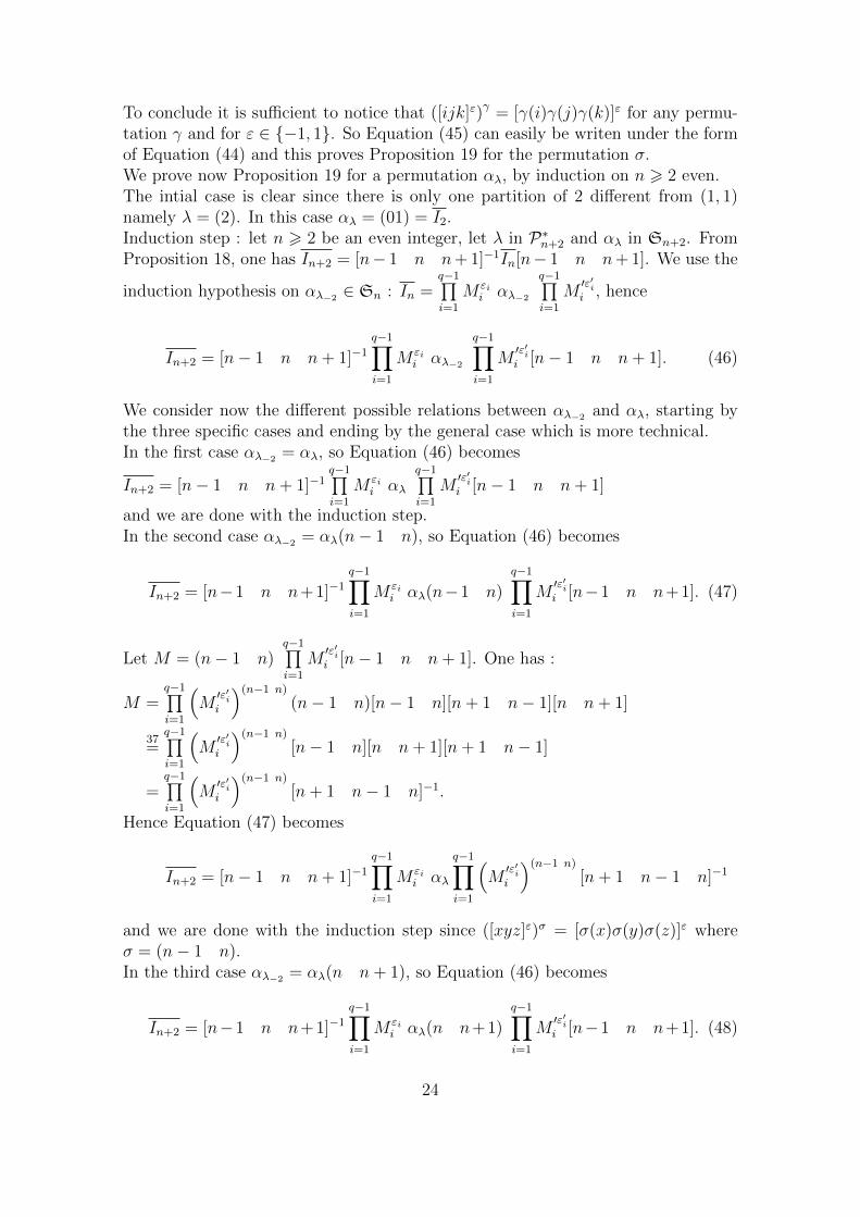
To conclude it is sufficient to notice that ([ijk]ε)γ = [γ(i)γ(j)γ(k)]ε for any permu-tation γ and for ε ∈ −1, 1. So Equation (45) can easily be writen under the formof Equation (44) and this proves Proposition 19 for the permutation σ.We prove now Proposition 19 for a permutation αλ, by induction on n > 2 even.The intial case is clear since there is only one partition of 2 different from (1, 1)namely λ = (2). In this case αλ = (01) = I2.Induction step : let n > 2 be an even integer, let λ in P∗n+2 and αλ in Sn+2. FromProposition 18, one has In+2 = [n− 1 n n+ 1]−1In[n− 1 n n+ 1]. We use the

induction hypothesis on αλ−2 ∈ Sn : In =q−1∏i=1

M εii αλ−2

q−1∏i=1

M′ε′ii , hence

In+2 = [n− 1 n n+ 1]−1q−1∏i=1

M εii αλ−2

q−1∏i=1

M′ε′ii [n− 1 n n+ 1]. (46)

We consider now the different possible relations between αλ−2 and αλ, starting bythe three specific cases and ending by the general case which is more technical.In the first case αλ−2 = αλ, so Equation (46) becomes

In+2 = [n− 1 n n+ 1]−1q−1∏i=1

M εii αλ

q−1∏i=1

M′ε′ii [n− 1 n n+ 1]

and we are done with the induction step.In the second case αλ−2 = αλ(n− 1 n), so Equation (46) becomes

In+2 = [n−1 n n+1]−1q−1∏i=1

M εii αλ(n−1 n)

q−1∏i=1

M′ε′ii [n−1 n n+1]. (47)

Let M = (n− 1 n)q−1∏i=1

M′ε′ii [n− 1 n n+ 1]. One has :

M =q−1∏i=1

(M′ε′ii

)(n−1 n)

(n− 1 n)[n− 1 n][n+ 1 n− 1][n n+ 1]

37=

q−1∏i=1

(M′ε′ii

)(n−1 n)

[n− 1 n][n n+ 1][n+ 1 n− 1]

=q−1∏i=1

(M′ε′ii

)(n−1 n)

[n+ 1 n− 1 n]−1.

Hence Equation (47) becomes

In+2 = [n− 1 n n+ 1]−1q−1∏i=1

M εii αλ

q−1∏i=1

(M′ε′ii

)(n−1 n)

[n+ 1 n− 1 n]−1

and we are done with the induction step since ([xyz]ε)σ = [σ(x)σ(y)σ(z)]ε whereσ = (n− 1 n).In the third case αλ−2 = αλ(n n+ 1), so Equation (46) becomes

In+2 = [n−1 n n+1]−1q−1∏i=1

M εii αλ(n n+1)

q−1∏i=1

M′ε′ii [n−1 n n+1]. (48)

24

Let M = (n n+ 1)q−1∏i=1

M′ε′ii [n− 1 n n+ 1]. One has :

M =q−1∏i=1

(M′ε′ii

)(n n+1)

(n n+ 1)[n− 1 n][n+ 1 n− 1][n n+ 1]

41=

q−1∏i=1

(M′ε′ii

)(n n+1)

[n n− 1][n− 1 n+ 1][n+ 1 n]

=q−1∏i=1

(M′ε′ii

)(n n+1)

[n+ 1 n n− 1]−1.

Hence Equation (48) becomes

In+2 = [n− 1 n n+ 1]−1q−1∏i=1

M εii αλ

q−1∏i=1

(M′ε′ii

)(n n+1)

[n+ 1 n n− 1]−1

and we are done with the induction step since ([xyz]ε)σ = [σ(x)σ(y)σ(z)]ε whereσ = (n n+ 1).In the general case, we start by conjugating each member of Equation (46) by(n n+ 1). Using the invariance of In by conjugation (Identity (34)), we get :

In+2 = (n n+1)[n−1 n n+1]−1q−1∏i=1

M εii αλ−2

q−1∏i=1

M′ε′ii [n−1 n n+1](n n+1).

(49)

On one hand, we have :(n n+ 1)[n− 1 n n+ 1]−1 = (n n+ 1)[n n+ 1][n+ 1 n− 1][[n− 1 n]

37= [n n+ 1][[n− 1 n][n+ 1 n− 1]= [n n+ 1 n− 1]

On the other hand we have :[n− 1 n n+ 1](n n+ 1) = [n− 1 n][n+ 1 n− 1][n n+ 1](n n+ 1).

36= [n+ 1 n− 1][n− 1 n][n n+ 1].= [n n+ 1 n− 1]−1

So Equation (49) becomes :

In+2 = [n n+ 1 n− 1]q−1∏i=1

M εii αλ−2

q−1∏i=1

M′ε′ii [n n+ 1 n− 1]−1

In the general case, one has :αλ−2 = αλ(n n+ 1)(n− 1 n) = αλ(n− 1 n)(n+ 1 n− 1), hence

In+2 = [n n+1 n−1]

q−1∏i=1

M εii αλ(n−1 n)(n+1 n−1)

q−1∏i=1

M′ε′ii [n n+1 n−1]−1.

(50)

Let M = (n− 1 n)(n+ 1 n− 1)q−1∏i=1

M′ε′ii [n n+ 1 n− 1]−1. One has :

M =q−1∏i=1

(M′ε′ii

)(n−1 n)(n+1 n−1)(n− 1 n)(n+ 1 n− 1)[n n+ 1 n− 1]−1

25

37=

q−1∏i=1

(M′ε′ii

)(n−1 n)(n+1 n−1)(n− 1 n)[n+ 1 n− 1][n n+ 1][n− 1 n]

41=

q−1∏i=1

(M′ε′ii

)(n−1 n)(n+1 n−1)[n− 1 n+ 1][n+ 1 n][n n− 1]

=q−1∏i=1

(M′ε′ii

)(n−1 n)(n+1 n−1)[n n− 1 n+ 1]−1.

Hence Equation (50) becomes :

In+2 = [n n+1 n−1]

q−1∏i=1

M εii αλ

q−1∏i=1

(M′ε′ii

)(n−1 n)(n+1 n−1)[n n−1 n+1]−1

and we are done with the induction step since ([xyz]ε)σ = [σ(x)σ(y)σ(z)]ε whereσ = (n− 1 n)(n+ 1 n− 1).

Actually the main interest of Proposition 19 is to give a way to compute easily adecomposition of σ in transvections, as described in the following proposition.

Proposition 20. Let n > 2 be an even integer. For any permutation matrix σ ofGLn(F2) different from In there exists n − 2 matrices M1, . . . ,Mn−2 of type [xyz]and n− 2 integers εi ∈ 1,−1 such that :

σ =n−2∏i=1

M εii (51)

Proof. Let σ be a permutation matrix of GLn(F2) different from In. Applying

Proposition 19 to σ−1 one has In =q−1∏i=1

M εii σ−1

q−1∏i=1

M′ε′ii . Hence σ = σIn =

q−1∏i=1

(M εii )σ

q−1∏i=1

M′ε′ii .

Since the proof of Proposition 19 is constructive, the method used in the proof ofProposition 20 gives an algorithm to decompose any matrix σ different from In in3(n − 2) transvections (see Figure 16 for an example). We conjecture that thisdecomposition is optimal and we checked it for n = 4.

26

Let n = 6 and σ = (503)(142) =

1 1 1 1 1 01 1 0 1 1 11 1 1 1 0 10 1 1 1 1 11 0 1 1 1 11 1 1 0 1 1

.

σ−1 = (305)(241). Let λ6 = (3, 3) be the cycle type of σ−1, then αλ6 = (012)(345).Let λ4 = (3, 1), then αλ4 = (012)(3) = αλ6(34)(53).Let λ2 = (2), then αλ2 = (01) = αλ4(12).I2 = αλ2I4 = [123]−1I2[123] = [123]−1αλ2 [123] = [123]−1αλ4(12)[123]I4 = [123]−1αλ4(12)[12][31][23] = [123]−1αλ4 [12][23][31] = [123]−1αλ4 [312]−1

I6 = [345]−1I4[345] = [345]−1[123]−1αλ4 [312]−1[345]I6 = [45][53][34][123]−1αλ6(34)(53)[312]−1[34][53][45]I6 = (45)[45][53][34][123]−1αλ6(34)(53)[312]−1[34][53][45](45)I6 = [45][34][53][123]−1αλ6(34)(53)[312]−1[53][34][45]

I6 = [453][123]−1αλ6 ([312]−1)(34)(53)

(34)(53)[53][34][45]I6 = [453][123]−1αλ6 [512]−1(34)[53][45][34]I6 = [453][123]−1αλ6 [512]−1[35][54][43]I6 = [453][123]−1αλ6 [512]−1[435]−1

σ−1 = αγλ6 where γ =

(0 1 2 3 4 53 0 5 2 4 1

), hence :

I6 = (I6)γ = ([453][123]−1)γσ−1([512]−1[435]−1)γ = [412][052]−1σ−1[105]−1[421]−1

σ = σI6 = ([412][052]−1)σ[105]−1[421]−1 = [241][301]−1[105]−1[421]−1

σ = [24][12][41][01][13][30][05][51][10][21][14][42]

Figure 16: Decomposition in transvections of a matrix of type σ.

27

6 Entanglement in CNOT gates circuits

The notion of entanglement is usually defined through the group of Stochastic LocalOperations assisted by Classical Communication denoted by SLOCC which is assim-ilated to the cartesian group product SL2(C)×n [27, 8]. Mathematically two states|ψ〉 and |ϕ〉 are SLOCC-equivalent if there exist n operators A1, . . . , An in SL2(C)such that A1 ⊗ · · · ⊗ An |ψ〉 = λ |ϕ〉 for some complex number λ. In other words,|ψ〉 and |ϕ〉 are SLOCC-equivalent if they are in the same orbit of GL2(C)×n actingon the Hilbert space C2⊗· · ·⊗C2. The SLOCC-equivalence of two states |ϕ〉 and |ψ〉has a physical interpretation as explained in [8] : |ϕ〉 and |ψ〉 can be interconvertedinto each other with non zero probability by n parties being able to coordinatetheir action by classical communication, each party acting separately on one of thequbits. The SLOCC-equivalence of two states |ϕ〉 and |ψ〉 implies that both statescan achiveve the same tasks (for instance in a communication protocol) but with aprobability of a success that may differ. In this sense the SLOCC-equivalence can beconsidered as a qualitative way of separating non equivalent quantum states.

Some states have a particular interest like the Greenberger-Horne-Zeilinger state[15]

|GHZn〉 =1√2

| ×n︷ ︸︸ ︷0 · · · 0〉+ |

×n︷ ︸︸ ︷1 · · · 1〉

=1√2

(|0〉⊗n + |1〉⊗n

)(n > 3) (52)

and the W-state [8]

|Wn〉 =1√n

(|10 · · · 0〉+ |010 · · · 0〉+ · · ·+ |0 · · · 01〉) (n > 3). (53)

These two states represent two non-equivalent kind of entanglements : they belongto distinct SLOCC orbits and thus cannot be interconverted into each other by localoperations (even probalistically). These states are particularly usefull because theyare required as a physical ressource to realize many specific tasks. For instance, inan anonymous network where the processors share the W-state, the leader electionproblem can be solved by a simple protocol whereas the GHZ-state is the only sharedstate that allows solution of distributed consensus [7]. The GHZ-state is also used inmany protocols in quantum cryptography, e.g. in secret sharing [17].

We denote by Hi the Hadamard gate (see Figure 2) applied on qubit i. For instance

in a 3-qubit system, H1 = I⊗ H⊗ I where I =

[1 00 1

]and H = 1√

2

[1 11 −1

]. In the

following we study the emergence of entanglement when a CNOT gates circuit actson a fully factorized state.

6.1 Creating a GHZ-state

The construction of the GHZ-state for n qubit is straightforward :

|GHZn〉 = Xn−1 n−2 . . . X21X10H0 |0〉⊗n . (54)

28

A simple computation proves Equation (54). Indeed one hasH0 |0 . . . 0〉 = 1√

2(|0 . . . 0〉+ |10 . . . 0〉) and Xn−1 n−2 . . . X21X10 |10 . . . 0〉 = |1 . . . 1〉.

If n = 4, Equation (54) corresponds to the circuit in Figure 17.

|0〉|0〉|0〉|0〉

H

|GHZ4〉

Figure 17: Using a circuit of cX4 to obtain |GHZ4〉.

6.2 The group cX3 and entanglement of a 3-qubit system

We prove that the group cX3 is powerful enough to generate any entanglement typefrom a completely factorized state. We use the method pioneered by Klyachko in[23] wherein he promoted the use of Algebraic Theory of Invariant. The statesof a SLOCC-orbit are characterized by their values on covariant polynomials. Let|ψ〉 =

∑i,j,k∈0,1

αijk |ijk〉 be a 3-qubit state. The simplest covariant associated to |ψ〉

is the trilinear form :

A =∑

i,j,k∈0,1

αijkxiyjzk. (55)

From A one computes three quadratic forms :

Bx(x0, x1) =

∣∣∣∣∣ ∂2A∂y0∂z0

∂2A∂y0∂z1

∂2A∂y1∂z0

∂2A∂y1∂z1

∣∣∣∣∣ , (56)

By(y0, y1) =

∣∣∣∣∣ ∂2A∂x0∂z0

∂2A∂x0∂z1

∂2A∂x1∂z0

∂2A∂x1∂z1

∣∣∣∣∣ , (57)

Bz(z0, z1) =

∣∣∣∣∣ ∂2A∂x0∂y0

∂2A∂x0∂y1

∂2A∂x1∂y0

∂2A∂x1∂y1

∣∣∣∣∣ . (58)

The catalectican is a trilinear form obtained by computing any of the three Jacobiansof A with one of the quadratic forms, which turns out to be the same,

C(x0, x1, y0, y1, z0, z1) =

∣∣∣∣ ∂A∂x0

∂A∂x1

∂Bx∂x0

∂Bx∂x1

∣∣∣∣ . (59)

29

The three quadratic forms Bx, By and Bz have the same discriminant ∆ which isthe last covariant polynomial we need to characterize the SLOCC-orbits :

∆(|ψ〉) = (α000α111 − α001α110 − α010α101 + α011α100)2

−4 (α000α011 − α001α010) (α100α111 − α101α110) .(60)

The polynomial ∆ is the generator of the algebra of invariant polynomials underthe action of SLOCC (i.e ∆(|ψ〉) = ∆(M |ψ〉) for any M ∈ SL2(C)×3). It is also theCayley hyperdeterminant of the trilinear binary form A [4].Let V := [Bx, By, Bz, C,∆] be a vector of covariants. We associate the binaryvector V [|ψ〉] := [[Bx(|ψ〉], [By(|ψ〉)], [Bz(|ψ〉)], [C(|ψ〉)], [∆(|ψ〉)]] to any state |ψ〉,where [P (|ψ〉)] = 0 if P (|ψ〉) = 0 and [P (|ψ〉)] = 1 if P (|ψ〉) 6= 0. The value ofV [|ψ〉] is sufficient to distinguish between the different orbits (see [18]). Results aresummarized in Table 3.

Orbit Symbols Representatives |ψ〉 V [|ψ〉]OV I |GHZ3〉 [1, 1, 1, 1, 1]OV |W3〉 [1, 1, 1, 1, 0]OIV 1√

2(|000〉+ |110〉) [0, 0, 1, 0, 0]

OIII 1√2(|000〉+ |101〉) [0, 1, 0, 0, 0]

OII 1√2(|000〉+ |011〉) [1, 0, 0, 0, 0]

OI |000〉 [0, 0, 0, 0, 0]

Table 3: The SLOCC orbits in a 3-qubit system.

For Equation (54) one has |GHZ3〉 = X21X10H0 |000〉 (orbitOV ) and it is easy to checkthat 1√

2(|000〉 + |011〉) = X21H1 |000〉 (orbit OII), 1√

2(|000〉 + |101〉) = X20H0 |000〉

(orbit OIII), and 1√2(|000〉+ |110〉) = X10H0 |000〉 (orbit OIV ).

In order to obtain a SLOCC-equivalent to |W3〉 we see from Table 3 that one hasto construct a state ψ such that ∆(|ψ〉) = 0 and C(x0, x1, y0, y1, z0, z1) 6= 0. Thiscan be done using only gates of the standard set of universal gates (Figure 2) asexplained in Proposition 21 (see Figure 18 for an example of circuit). Note that theconstruction involves CNOT gates circuits that have matrices of type [ijk] (describedin Subsection 5.3).

Proposition 21. Let X[ijk] = XijXkiXjk where i, j, k are distinct integers in 0, 1, 2and k 6= 2. The state

X[ijk](T⊗ T⊗ S)H⊗3 |000〉 (61)

is SLOCC-equivalent to |W3〉.

Proof. Let q = eiπ4 and let |ψ(k0,k1,...,k7)〉 = 1√

8

(qk0 |000〉+ qk1 |001〉+ · · ·+ qk7 |111〉

)where ki is an integer. A simple calculation shows that (T ⊗ T ⊗ S)H⊗3 |000〉 =|ψ(0,2,1,3,1,3,2,4)〉. Then we compute the values of polynomials ∆ (Formula (60)) and

30

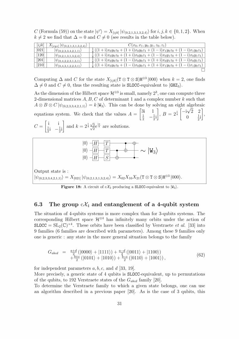
C (Formula (59)) on the state |ψ′〉 = X[ijk] |ψ(0,2,1,3,1,3,2,4)〉 for i, j, k ∈ 0, 1, 2. Whenk 6= 2 we find that ∆ = 0 and C 6= 0 (see results in the table below).

[ijk] X[xyz] |ψ(0,2,1,3,1,3,2,4)〉 C(x0, x1, y0, y1, z0, z1)[021] |ψ(0,2,3,3,4,2,1,1)〉 1

8 ((1 + i)x0y0z0 + (1 + i)x0y0z1 + (1− i)x1y0z0 + (1− i)x1y0z1)[120] |ψ(0,2,1,3,1,3,2,4)〉 1

8 ((1 + i)x0y0z0 + (1 + i)x0y0z1 + (1− i)x0y1z0 + (1− i)x0y1z1)[201] |ψ(0,4,2,2,3,1,3,1)〉 1

8 ((1 + i)x0y0z0 + (1− i)x0y0z1 + (1 + i)x0y1z0 + (1− i)x0y1z1)[210] |ψ(0,4,3,1,2,2,3,1)〉 1

8 ((1 + i)x0y0z0 + (1− i)x0y0z1 + (1 + i)x1y0z0 + (1− i)x1y0z1)

Computing ∆ and C for the state X[ijk](T ⊗ T ⊗ S)H⊗3 |000〉 when k = 2, one finds∆ 6= 0 and C 6= 0, thus the resulting state is SLOCC-equivalent to |GHZ3〉.As the dimension of the Hilbert spaceH⊗3 is small, namely 23, one can compute three2-dimensional matrices A,B,C of determinant 1 and a complex number k such thatA ⊗ B ⊗ C |ψ(0,2,3,3,4,2,1,1)〉 = k |W3〉. This can be done by solving an eight algebraic

equations system. We check that the values A =

[3i 112−1

2i

], B = 2

14

[−i√

2 20 1

2i

],

C =

[i i12i −1

2i

]and k = 2

14

√3√2e

iπ4 are solutions.

|0〉|0〉|0〉

H

H

H

T

T

S

∼ |W3〉

Output state is :|ψ(0,2,3,3,4,2,1,1)〉 = X[021] |ψ(0,2,1,3,1,3,2,4)〉 = X02X10X21(T⊗ T⊗ S)H⊗3 |000〉.

Figure 18: A circuit of cX3 producing a SLOCC-equivalent to |W3〉.

6.3 The group cX4 and entanglement of a 4-qubit system

The situation of 4-qubits systems is more complex than for 3-qubits systems. Thecorresponding Hilbert space H⊗4 has infinitely many orbits under the action ofSLOCC = SL2(C)×4. These orbits have been classified by Verstraete et al. [33] into9 families (6 families are described with parameters). Among these 9 families onlyone is generic : any state in the more general situation belongs to the family

Gabcd = a+d2

(|0000〉+ |1111〉) + a−d2

(|0011〉+ |1100〉)+ b+c

2(|0101〉+ |1010〉) + b−c

2(|0110〉+ |1001〉) , (62)

for independent parameters a, b, c, and d [33, 19].More precisely, a generic state of 4 qubits is SLOCC-equivalent, up to permutationsof the qubits, to 192 Verstraete states of the Gabcd family [20].To determine the Verstraete family to which a given state belongs, one can usean algorithm described in a previous paper [20]. As is the case of 3 qubits, this

31

algorithm is based on the evaluation of some covariants polynomials (see AppendixA). We do not recall the algorithm since it is not usefull to understand the presentpaper.

Let |ψ〉 =∑

i,j,k,`∈0,1αijk` |ijk`〉 be a 4-qubit state. The algebra of SLOCC-invariant

polynomials is freely generated by the four following polynomials [25]:

• The smallest degree invariant

B :=∑

06i1,i2,i361

(−1)i1+i2+i3α0i1i2i3α1(1−i1)(1−i2)(1−i3), (63)

• Two polynomials of degree 4

L :=

∣∣∣∣∣∣∣∣α0000 α0010 α0001 α0011

α1000 α1010 α1001 α1011

α0100 α0110 α0101 α0111

α1100 α1110 α1101 α1111

∣∣∣∣∣∣∣∣ (64)

and

M :=

∣∣∣∣∣∣∣∣α0000 α0001 α0100 α0101

α1000 α1001 α1100 α1101

α0010 α0011 α0110 α0111

α1010 α1011 α1110 α1111

∣∣∣∣∣∣∣∣ . (65)

• and a polynomial of degree 6 defined by Dxy = − det(Bxy) where Bxy is the3× 3 matrix satisfying

[x20, x0x1, x

21

]Bxy

y20y0y1y21

= det

(∂2

∂zi∂tjA

)(66)

with A =∑

i,j,k,`∈0,1αijk`xiyjzkt` being the quadrilinear binary form associated

to the state |ψ〉.

Using the generators B,L,M and Dxy, one can build ∆, an invariant polynomial ofdegree 24 that plays an important role in the quantitative and qualitative study ofentanglement [28, 26]. As described in [19] and [25], ∆ is the discriminant of any ofthe quartics

Q1 = x4−2Bx3y+ (B2 + 2L+ 4M)x2y2 + 4(Dxy−B(M +1

2L))xy3 +L2y4, (67)

Q2 = x4 − 2Bx3y + (B2 − 4L− 2M)x2y2 + (4Dxy − 2MB)xy3 +M2y4, (68)

32

and

Q3 = x4− 2Bx3y + (B2 + 2L− 2M)x2y2− (2(L+M)B− 4Dxy)xy3 +N2y4. (69)

We recall that, for a quartic Q = αx4−4βx3y+6γx2y2−4δxy3+ωy4, the discriminantcan be computed as

∆ = I32 − 27I23 (70)

where I2 = αω − 4βδ + 3γ2 and I3 = αγω − αδ2 − ωβ2 − γ3 + 2βγδ.It appears that ∆ is the Cayley hyperdeterminant (in the sense of Gelfand et al.[12]) of A [25]. In [26], Miyake showed that the more generic entanglement holdsonly for the states |ψ〉 such that ∆(|ψ〉) 6= 0. Moreover any generically entangledstate is equivalent to a state of the Verstraete Gabcd family [25, Appendix A]. So onecan consider ∆ as a qualitative measure of entanglement : an entangled state (i.e.not factorized state) is generically entangled if ∆ 6= 0.In the case of 3 qubits, ∆(|GHZ3〉) 6= 0 (see Table 3). Using (60) one checks easilythat ∆(|GHZ3〉) = 1

4. So the state |GHZ3〉 is generically entangled. In the 4 qubits case

one computes ∆(|GHZ4〉) = 0 using (70). Hence, suprisingly, |GHZ4〉 is not genericallyentangled and this result can be generalized : in [2] Appendix C we proved that, forany k > 3, ∆(|GHZk〉) = 0.In this context we ask ourselves if it is possible to find a 4-qubit CNOT gates circuitthat takes as input a completely factorized state and output a generically entangledstate. The following statement answers the question.

Theorem 22. The state |BL〉 := X01X20X03X10(T⊗ S⊗ S⊗ S)H⊗4 |0000〉 is gener-ically entangled. It is produced by the circuit :

|0〉|0〉|0〉|0〉

H

H

H

H

T

S

S

S

Proof. Using formula (70) one computes ∆(|BL〉) = − 1

224' −5, 96× 10−8.

According to Miyake [28], the value of |∆| can be considered as a measure of entan-glement. So a state with the most amount of generic entanglement can be definedas a state that maximize |∆|. In the 4-qubits case the maximal value of |∆| is1

2839' 1, 98 × 10−7 [5] and the mean is around 1.32 × 10−9 (value based on 10000

random states [1]). So the amount of generic entanglement in the state |BL〉 is notmaximal, although much higher than the mean.A few states are known to maximize |∆| : |L〉 [16, 14, 5], |HD〉 [1] and |M2222〉(Jaffali, phd thesis). Figure 19 gives the definition of these states. It seems inter-esting to know if it is possible, starting from a fully factorized state, to reach one ofthese 3 states by a 4-qubit CNOT gates circuit. To answer this question we proceedas follows. We start from a fully factorized state

|F (u)〉 := (a0 |0〉+a1 |1〉)⊗ (b0 |0〉+b1 |1〉)⊗ (c0 |0〉+c1 |1〉)⊗ (d0 |0〉+d1 |1〉) (71)

33

where u := [a0, a1, b0, b1, c0, c1, d0, d1] is a vector of complex numbers. Then, for eachcircuit C in cX4, we compute C |F (u)〉 and we check that the equation C |F (u)〉 =|ψ〉 where |ψ〉 ∈ |L〉 , |HD〉 , |M2222〉 has no solution. This can be done in afew seconds using Maple 2020 (X86 64 LINUX). The corresponding script can bedownloaded at https://github.com/marcbataille/cnot-circuits. Hence theanswer to our question is negative.Note that the question whether a state different from |L〉, |HD〉, or |M2222〉 thathas maximal generic entanglement can be produced under the same constraints (i.e.factorized state plus 4-qubit CNOT gates circuit) remains open, however.

|L〉 =1√3

(|u0〉+ ω |u1〉+ ω2 |u2〉 (72)

with: |u0〉 = 12(|0000〉+ |0011〉+ |1100〉+ |1111〉)

|u1〉 = 12(|0000〉 − |0011〉 − |1100〉+ |1111〉)

|u2〉 = 12(|0101〉+ |0110〉+ |1001〉+ |1010〉)

ω = e2iπ3

|HD〉 =1√6

(|0001〉+ |0010〉+ |0100〉+ |1000〉+√

2 |1111〉). (73)

|M2222〉 =1√6|v1〉+

√6

4|v1〉+

1√2|v3〉 (74)

with: |v1〉 = 1√6(|0000〉+ |0101〉 − |0110〉 − |1001〉+ |1010〉+ |1111〉)

|v2〉 = 1√2(|0011〉+ |1100〉)

|v3〉 = 1√2(− |0001〉+|0010〉−|0100〉+|0111〉+|1000〉−|1011〉+|1101〉−|1110〉)

Figure 19: 4-qubits states for which |∆| is maximal.

We examine now whether it is possible to obtain a SLOCC-equivalent to |W4〉 =12(|0001〉+|0010〉+|0100〉+|1000〉) when a CNOT gates circuit acts on a fully factorized

state. The SLOCC-orbit of |W4〉 belongs to the null cone, which is the algebraicvariety defined by the vanishing of all invariants (i.e. B(|ψ〉) = L(|ψ〉) = M(|ψ〉) =Dxy(|ψ〉) = 0). The null cone contains 31 SLOCC-orbits and the orbit of |W4〉 ischaraterized, inside the null cone, by the evaluation of a vector of 8 polynomialcovariants A,PB, P

1C , P

2C , P

1D, P

2D, PF , PL whose definitions have been relegated to

Appendix A (see [19, Section III] for more details). More precisely, one has thefollowing criterion :

Proposition 23. Let V1 := [B,L,M,Dxy] and V2 := [A,PB, P1C , P

2C , P

1D, P

2D, PF , PL]

then |ψ〉 is in the SLOCC-orbit of |W4〉 if and only if V 1[|ψ〉] = [0, 0, 0, 0] and V 2[|ψ〉] =[1, 1, 1, 1, 0, 0, 0, 0].

The use of this criterion makes it possible to answer our initial question :

34

Theorem 24. The SLOCC-orbit of |W4〉 cannot be reached when cX4 acts on a fullyfactorized state |F (u)〉.

Proof. We prove that, for any circuit C ∈ cX4, the state |ψ(u)〉 = C |F (u)〉 cannotbe in the SLOCC-orbit of |W4〉. The algorithm is the following. For each C in cX4 wesolve the system B(|ψ(u)〉) = L(|ψ(u)〉) = M(|ψ(u)〉) = Dxy(|ψ(u)〉) = 0. The solu-tions are parametrized vectors |ψ1(u)〉 , . . . , |ψn(u)〉. Then for each solution |ψi(u)〉we solve the system P 1

D(|ψi(u)〉) = P 2D(|ψi(u)〉 = PF (|ψi(u)〉) = PL(|ψi(u)〉 = 0

and for each solution |ψij(u)〉 we compute P 2C : we check that the polynomial

P 2C(|ψij(u)〉) is null for any u,C, i, j. We deduce from Proposition 23 that |ψ(u)〉 is

not SLOCC-equivalent to |W4〉. The Maple script that implements this algorithm canbe downloaded at https://github.com/marcbataille/cnot-circuits and needsa few hours to be executed.

7 Conclusion and perspectives

The omnipresence and great significance of CNOT gates in quantum computationwas our main motivation to better understand the quantum circuits build with thesegates. First we described the link between CNOT gates circuits of n qubits and a clas-sical group, namely GLn(F2) = SLn(F2). From there we deduced some simplificationrules and applied our results to optimization and reduction problems. In Section 4we proposed some polynomial heuristics to reduce circuits in the general case and inSection 5 we described a few algorithms to optimize circuits in some special cases.Finally we studied some issues about entanglement and proposed simple construc-tions to produce some usefull entangled states. Optimization and entanglement areindeed two central topics in QIT since they are related to some important issues onthe way to a reliable and functional quantum machine : optimization of circuits forscalable quantum computing and production of entanglement as a physical resourcein quantum communication protocols.As far as we know, a complete study of CNOT gates circuits does not exist yet inthe litterature and we hope the results and conjectures contained in this paper willcontribute to fill a part of this gap. We believe that the subject is rich and deservescertainly further investigations. In what follows we try to sketch some directionsthat future works on this subject could take.

Regarding to the optimization problem of CNOT gates circuits, it seems to us thatthe diversity of situations and methods described in Section 5 tends to show that apolynomial optimization algorithm for the general case, if it ever exists, will be hardto find out. In our opinion, a more realistic and feasible approach should be a mix ofheuristics for the general case (as the Gauss-Jordan algorithm or the UTD algorithmdescribed in Section 4) combined with a rich atlas of various methods to optimizeor to reduce circuits in special cases (as the atlas we started to built in Section5). Concerning heuristics in the general case, it is clear that the bound of n2 gatesresulting from the Gauss-Jordan algorithm (Proposition 10) has to be improved bythe use of another algorithm, since it is still far from the (probably) optimal linearbound of 3(n−1) gates given by Conjecture 12. Certainly, a constructive proof of this

35

conjecture would be a big step towards a better understanding of the optimizationproblem. We will continue to investigate technics of reduction in future works.

The study of the emergence of entanglement in CNOT gates circuits done in Section6 highlights the interest and utility of this tool especially in the case of 3 or 4 qubitssystems. When the number of qubits is greater than 4, it would be interestingto know whether it is possible to create generic entanglement as in the 4 qubitscase (Theorem 22). Unfortunately, from 5 qubits the hyperdeterminant is too hugeto be computed in a suitable form. However its nullity can be tested thanks toits interpretation in terms of solution of a system of equations [12, p. 445] : if

A =∑

06i,j,k,l,n61

αijklnxiyjzktlsn is the ground form associated to the five qubits state

|ϕ〉 =∑

06i,j,k,l,n61

αijkln|ijkln〉, the condition ∆(|ϕ〉) = 0 means that the system

Sϕ := A =d

dx0A =

d

dx1A =

d

dy0A =

d

dy1A = · · · = d

ds0A =

d

ds1A = 0 (75)

has a solution x0, x1, y0, y1, . . . , s0, s1 in the variables x0, x1, y0, y1, . . . , s0, s1 such that(x0, x1), (y0, y1), . . . , (s0, s1) 6= (0, 0). Such a solution is called non trivial. Hence apossible approach to show that a state |ψ〉 is generically entangled when n > 4 is toprove that the corresponding system has no solution apart from the trivial solutions.

References

[1] Daniel Alsina. Phd thesis: Multipartite entanglement and quantum algorithms,2017.

[2] Marc Bataille and Jean-Gabriel Luque. Quantum circuits of cZ and SWAPgates: optimization and entanglement. Journal of Physics A: Mathematicaland Theoretical, 52(32):325302, jul 2019.

[3] Charles H. Bennett and Stephen J. Wiesner. Communication via one- and two-particle operators on einstein-podolsky-rosen states. Phys. Rev. Lett., 69:2881–2884, Nov 1992.

[4] Arthur Cayley. Memoire sur les hyperdeterminants. Journal fur die reine undangewandte Mathematik, 30:1–37, 1846.

[5] Lin Chen and Dragomir . okovi. Proof of the Gour-Wallach conjecture. PhysicalReview A, 88(4), oct 2013.

[6] Richard Cleve, Daniel Gottesman, and Hoi-Kwong Lo. How to share a quantumsecret. Physical Review Letters, 83(3):648651, Jul 1999.

[7] Ellie D’Hondt and Prakash Panangaden. The computational power of the Wand GHZ states, 2004.

36

[8] Wolfgang Dur, Guifre Vidal, and Cirac J. Ignacio. Three qubits can be entan-gled in two inequivalent ways. Physical Review A, 62:062314, 2000.

[9] A. Einstein, B. Podolsky, and N. Rosen. Can quantum-mechanical descriptionof physical reality be considered complete ? Physical Review, Vol. 47, 1935.

[10] Ekert. Quantum cryptography based on Bell’s theorem. Physical review letters,67 6:661–663, 1991.

[11] Akira Furusawa, Jens Lykke Sorensen, Samuel L. Braunstein, Christopher AFuchs, H. Jeff Kimble, and Eugene S. Polzik. Unconditional Quantum Telepor-tation. Science, 282:706, October 1998.

[12] Israel M Gelfand, Mikhail M. Kapranov, and Zelevisnky Andrei V. Discrimi-nants, Resultants and Multidimensional Determinant. Birkhauser, 1992.

[13] Gilad Gour and Nolan R. Wallach. Entanglement of subspaces and error-correcting codes. Physical Review A, 76(4), Oct 2007.

[14] Gilad Gour and Nolan R. Wallach. On symmetric SL-invariant polynomials infour qubits, 2012.

[15] Daniel M. Greenberger, Michael A. Horne, and Anton Zeilinger. Bell’s theoremwithout inequalities. American Journal of Physics, 58 (12):1131, 1990.

[16] A. Higuchi and A. Sudbery. How entangled can two couples get? PhysicsLetters A, 273(4):213 – 217, 2000.

[17] Mark Hillery, Vladimr Buek, and Andr Berthiaume. Quantum secret sharing.Physical Review A, 59(3):18291834, Mar 1999.

[18] Frederic Holweck, Jean-Gabriel Luque, and Thibon Jean-Yves. Geometric de-scriptions of entangled states by auxiliary varieties. Journal of MathematicalPhysics, 53 (10):102203, 2012.

[19] Frederic Holweck, Jean-Gabriel Luque, and Thibon Jean-Yves. Entanglementof four qubit systems: A geometric atlas with polynomial compass I (the finiteworld). Journal of Mathematical Physics, 55 (1):012202, 2014.

[20] Frederic Holweck, Jean-Gabriel Luque, and Thibon Jean-Yves. Entanglementof four-qubit systems: a geometric atlas with polynomial compass II (the tameworld). Journal of Mathematical Physics, 58 (2):022201, 2017.

[21] John Hopcroft and Robert Tarjan. Algorithm 447: Efficient algorithms forgraph manipulation. Commun. ACM, 16(6):372378, June 1973.

[22] Ryszard Horodecki, Pawe l Horodecki, Micha l Horodecki, and Karol Horodecki.Quantum entanglement. Rev. Mod. Phys., 81:865–942, Jun 2009.

[23] Alexander Klyachko. Coherent states, entanglement, and geometric invarianttheory. arXiv:quant-ph/0206012v1.

37

[24] Norbert M. Linke, Dmitri Maslov, Martin Roetteler, Shantanu Debnath, Car-oline Figgatt, Kevin A. Landsman, Kenneth Wright, and Monroe Christopher.Experimental comparison of two quantum computing architectures. Proceed-ings of the National Academy of Sciences of the United States of America, 114(13):3305–3310, March 2017.

[25] Jean-Gabriel Luque and Jean-Yves Thibon. The polynomial invariants of fourqubits. Phys. Rev. A, 67:042303, 2003.

[26] Akimasa Miyake. Classification of multipartite entangled states by multidimen-sional determinant. Phys. Rev. A, 67:012108, 2003.

[27] Akimasa Miyake. Multipartite entanglement under stochastic local operationsand classical communication, 2004.

[28] Akimasa Miyake and Miki Wadati. Multipartite entanglement and hyperdeter-minants. Quantum Information and Computation, 2:540–555, 2002.

[29] Michael A. Nielsen and Isaac L. Chuang. Quantum Computation and Quan-tum Information: 10th Anniversary Edition. Cambridge University Press, NewYork, NY, USA, 10th edition, 2011.

[30] Stefano Pirandola, Jens Eisert, Christian Weedbrook, Akira Furusawa, andSamuel L. Braunstein. Advances in quantum teleportation. Nature Photonics,9:641–652, October 2015.

[31] Robert Steinberg. Lectures on Chevalley Groups. University Lecture Series 66.American Mathematical Society, 2016.

[32] Lev Vaidman. Teleportation of quantum states. Physical Review A, 49:1473–1476, February 1994.

[33] Frank Verstraete, Jeronen Dehaene, Bart De Moor, and Henri Verschelde. Fourqubits can be entangled in nine different ways. Phys. Rev. A, 65:052112, 2002.

[34] Robert Wilson. The Finite Simple Groups. Springer London Ltd, 2009.

[35] K. Wright, K. M. Beck, S. Debnath, J. M. Amini, Y. Nam, N. Grzesiak, J.-S.Chen, N. C. Pisenti, M. Chmielewski, C. Collins, and et al. Benchmarking an11-qubit quantum computer. Nature Communications, 10(1), Nov 2019.

[36] D. M. Zajac, T. M. Hazard, X. Mi, E. Nielsen, and J. R. Petta. Scalable gatearchitecture for a one-dimensional array of semiconductor spin qubits. Phys.Rev. Applied, 6:054013, Nov 2016.

38

A Some covariant polynomials associated to 4 qubit

systems

In this section, we shall explain how to compute the polynomials which are usedto determine the SLOCC-orbit of |W4〉 inside the null cone (Section 6.3). We shallfirst recall the definition of the transvection of two multi-binary forms on the binaryvariables x(1) = (x

(1)0 , x

(1)1 ), . . . , x(p) = (x

(p)0 , x

(p)1 )

(f, g)i1,...,ip = tr Ωi1x(1)

. . .Ωipx(p)

f(x′(1), . . . , x′(p))g(x′′(1), . . . , x′′(p)), (76)

where Ω is the Cayley operator

Ωx =

∣∣∣∣∣ ∂∂x′0

∂∂x′′0

∂∂x′1

∂∂x′′1

∣∣∣∣∣and tr sends each variables x′, x′′ on x (erases ′ and ′′). In [18], we give a list ofgenerators of the algebra of covariant polynomials for 4 qubits systems which areobtained by transvection from the ground form

A =∑i,j,k,`

αi,j,k,lxiyjzkt`.

Here we give formulas for some of the polynomials which are used in the paper.

Symbol TransvectantB2200

12(A,A)0011

B202012(A,A)0101

B200212(A,A)0110

B022012(A,A)1001

B020212(A,A)1010

B002212(A,A)1100

Symbol TransvectantC1

1111 (A,B2200)1100 + (A,B0022)

0011

C311113

((A,B2200)0100 + (A,B2020)

0010 + (A,B2002)0001)

C131113

((A,B2200)1000 + (A,B0220)

0010 + (A,B0202)0001)

C113113

((A,B2020)1000 + (A,B0220)

0100 + (A,B0022)0001)

C111313

((A,B2002)1000 + (A,B0202)

0100 + (A,B0022)0010)

Symbol TransvectantD2200 (A,C1

1111)0011

D2020 (A,C11111)

0101

D2002 (A,C11111)

0110

D0220 (A,C11111)

1001

D0202 (A,C11111)

1010

D0022 (A,C1111)1100

D4000 (A,C3111)0111

D0400 (A,C1311)1011

D0040 (A,C1131)1101

D0004 (A,C1113)1110

Symbol TransvectantE1

3111 (A,D2200)0100 + (A,D2020)

0010 + (A,D2002)0001

E11311 (A,D2200)

1000 + (A,D0220)0010 + (A,D0202)

0001

E11131 (A,D2020)

1000 + (A,D0220)0100 + (A,D0022)

0001

E11113 (A,D2002)

1000 + (A,D0202)0100 + (A,D0022)

0010

Symbol TransvectantF4200 (A,E1

3111)0011

F4020 (A,E13111)

0101

F4002 (A,E13111)

0110

F0420 (A,E11311)

1001

F0402 (A,E11311)

1010

F0042 (A,E11131)

1100

F2400 (A,E11311)

0011

F2040 (A,E11131)

0101

F2004 (A,E11113)

0110

F0240 (A,E11131)

1001

F0204 (A,E11113)

1010

F0024 (A,E11113)

1100

39

Symbol TransvectantG5111 (A,F4002)

0001 + (A,F4020)0010 + (A,F4200)

0100

G1511 (A,F0402)0001 + (A,F0420)

0010 + (A,F2400)1000

G1151 (A,F0042)0001 + (A,F0240)

0100 + (A,F2040)1000

G1115 (A,F0204)0100 + (A,F0024)

0010 + (A,F2004)1000

Symbol TransvectantH4200 (A,G5111)

1011

H4020 (A,G5111)1101

H4002 (A,G5111)1110

H0420 (A,G1511)1101

H0402 (A,G1511)1110

H0042 (A,G1151)1110

H2400 (A,G11511)

0111

H2040 (A,G1151)0111

H2004 (A,G11115)

0111

H0240 (A,G1151)1011

H0204 (A,G1115)1011

H0024 (A,G11115)

1101

Symbol TransvectantI15111 (A,H4020)

0010 + (A,H4200)0100 + (A,H4002)

0001

I11511 (A,H0420)0010 + (A,H2400)

1000 + (A,H4002)0001

I11151 (A,H0240)0100 + (A,H2040)

1000 + (A,H0042)0001

I11115 (A,H0204)0100 + (A,H2004)

1000 + (A,H0024)0010

Symbol TransvectantJ4200 (A, I15111)

1011

J4020 (A, I15111)1101

J4002 (A, I15111)1110

J0420 (A, I11511)1101

J0402 (A, I11511)1110

J0042 (A, I11151)1110

J2400 (A, I11511)0111

J2040 (A, I11151)0111

J2004 (A, I11115)0111

J0240 (A, I11151)1011

J0204 (A, I11115)1011

J0024 (A, I11115)1101

Symbol TransvectantK5111 = (A, J4200)

0100 − (A, J4020)0010 + (A, J4002)

0001

K1511 = (A, J2400)1000 − (A, J0420)

0010 + (A, J0402)0001

K1151 = (A, J2040)1000 − (A, J0240)

0100 + (A, J0042)0001

K1115 = (A, J2004)1000 − (A, J0204)

0110 + (A, J0024)0010

Symbol TransvectantL6000 = (A,K5111)

0111

L0600 = (A,K1511)1011

L0060 = (A,K1151)1101

L0006 = (A,K1115)1110

We use the following polynomials in order to characterize the |W4〉 SLOCC-orbit:

PB := B2200 +B2020 +B2002 +B0220 +B0202 +B0022,

P 1C := C3111 + C1311 + C1131 + C1113,

P 2C := C3111C1311C1131C1113,

P 1D := D4000 +D0400 +D0040 +D0004,

P 2D := D2200 +D2020 +D2002 +D0220 +D0202 +D0022,

PF := F 12220 + F 1

2202 + F 12022 + F 1

0222,

PL := L6000 + L0600 + L0060 + L0006.

40