Quantum Circuits for Measuring Levin-Wen Operators

N. E. Bonesteel1 and D. P. DiVincenzo2,3,41Department of Physics and NHMFL, Florida State University, Tallahassee, Florida 32310, USA

2Institute for Quantum Information, RWTH Aachen University, D-52056 Aachen, Germany3Peter Grunberg Institute II, Theoretical Nanoelectronics, Forschungzentrum Julich, Julich, Germany

4Julich-Aachen Research Alliance (JARA), Fundamentals of Future Information Technologies

We construct quantum circuits for measuring the commuting set of vertex and plaquette operatorsthat appear in the Levin-Wen model for doubled Fibonacci anyons. Such measurements can beviewed as syndrome measurements for the quantum error-correcting code defined by the groundstates of this model (the Fibonacci code). We quantify the complexity of these circuits with gatecounts using different universal gate sets and find these measurements become significantly easierto perform if n-qubit Toffoli gates with n = 3, 4 and 5 can be carried out directly. In additionto measurement circuits, we construct simplified quantum circuits requiring only a few qubits thatcan be used to verify that certain self-consistency conditions, including the pentagon equation, aresatisfied by the Fibonacci code.

I. INTRODUCTION

The ground states of certain two-dimensional latticeHamiltonians of a type first introduced by Kitaev1 can beused as quantum error-correcting codes known as surfacecodes. Quantum information can be stored and protectedusing these codes when they are defined on lattices withholes (defects).2 Fault-tolerant gates can then be carriedout either transversally or by deforming the code in orderto braid these defects while staying entirely within thecode subspace.3–5 One downside to using the Kitaev sur-face codes, for which defects behave as Abelian anyons,is that to realize a universal set of fault-tolerant gatesat least one gate using a resource costly “magic state”distillation process6 is required. The same is true forfault-tolerant quantum computation using the so-calledcolor codes.7–11 Nevertheless, quantum computation us-ing these surface codes has a number of appealing fea-tures, notably the need for only nearest-neighbor gatesbetween qubits in a two-dimensional array and high errorthresholds, e.g. ∼ 1% for the Kitaev surface code.3–5,12

Recently Konig, Kuperberg, and Reichardt13 (KKR)outlined a method for fault-tolerant quantum computa-tion using non-Abelian surface codes. These codes, whichare defined mathematically in terms of the Turaev-Virotopological invariants for 3-manifolds,14 can be viewedphysically as ground states of Levin-Wen models,15 two-dimensional lattice models which generalize the Kitaevmodel.16 These models can be used to realize so-called“doubled” versions of any consistent anyon theory, in-cluding theories of non-Abelian anyons for which braid-ing is universal for quantum computation. The simplestsuch universal anyons are the Fibonacci anyons. Herewe refer to the corresponding Levin-Wen model as theFibonacci Levin-Wen model and, following KKR,13 referto the ground states of this model as the Fibonacci code.As shown in Ref. 13, when using the Fibonacci code,Fibonacci anyons can be associated with holes in the lat-tice subject to certain boundary conditions and properinitialization. These Fibonacci anyons can then be used

to encode logical qubits and universal quantum compu-tation can be carried out purely by braiding them,17–19

without the need for magic state distillation.The Levin-Wen models are defined by a set of com-

muting vertex and plaquette projection operators whichact on qubits (more generally, qudits) associated with theedges of a two-dimensional trivalent lattice. When usingthe ground states of these models as quantum codes itwill be necessary to continually measure these vertex andplaquette operators in order to check for errors, whichwould then have to be corrected without disturbing thequantum information stored in the topological degreesof freedom of the code. For the Kitaev surface code,quantum circuits which can be used to measure these op-erators are known and are fairly straightforward.20 Foreither an n-sided plaquette, or a vertex where n edgesmeet, these measurement circuits each require a singleinitialized syndrome qubit which is measured after car-rying out n controlled-NOT (CNOT) gates.

The simplicity of the quantum circuits used to measurethe vertex and plaquette operators for the Kitaev surfacecode reflects the Abelian nature of this code. It is nat-ural to ask how complex the quantum circuits need tobe to measure the vertex and plaquette operators for thenon-Abelian Fibonacci code. In this paper we presentexplicit quantum circuits for performing such measure-ments. These circuits are built in part out of smaller cir-cuits which carry out unitary transformations which havebeen described both in KKR13 and, in the context of en-tanglement renormalization, in Ref. 21. Our goal here isto explicitly construct these circuits in terms of standardelements (Toffoli gates, CNOT gates and single-qubit ro-tations) in an attempt to quantify their complexity.

The purpose of this work is not to argue that non-Abelian surface codes are viable competitors to the Ki-taev surface code. Indeed, we share the view of manyin the field that quantum computation using the Kitaevsurface code, given its clear advantages over other fault-tolerant quantum computation schemes, may well pro-vide the best practical route to building a functioningquantum computer.5,22 Here our goal is the more modest

arX

iv:1

206.

6048

v3 [

quan

t-ph

] 1

6 O

ct 2

012

2

i'n-1 in-1

i j

k v vQ ijkδ= i

j

k v

sBp ∑′′′′

−′′′′

−

−

−=

nn

nn

nniiii

nniiiisiiii aaaaB

121

121

121)( 121

,,

p

an-1

a1

a3

a2 i1 p

an

i2

in

an-1

a1

a3

a2 i'1 p

an

i'2

i'n

0=

1=

a) b)

FIG. 1: (Color online) (a) Example of a trivalent lattice (in this case a honeycomb lattice) on which the Levin-Wen modelcan be defined. For the Fibonacci Levin-Wen model a qubit is associated with each edge. A particular state which satisfiesthe vertex constraint Qv = 1 on each vertex for this model is shown. Thick edges indicate qubits in the state |1〉, thin edgesindicate qubits in the state |0〉. (b) Action of the vertex operator Qv on the three qubits on the edges connected to a trivalentvertex, and of the plaquette operators Bsp on the 2n qubits associated with an n-sided plaquette.

one of making a first pass at determining the complexityof syndrome extraction for the significantly less well un-derstood Fibonacci code, which we believe is of intrinsicinterest in its own right. An additional goal of this workis to begin developing a “dictionary” for translating themathematical structures which appear in general anyontheories into interesting quantum circuits, some of whichwe find require only a few qubits and might feasibly becarried out experimentally in the near future.

II. LEVIN-WEN MODELS AND THEFIBONACCI CODE

The Levin-Wen models15 are defined on two-dimensional trivalent lattices such as the hexagonal lat-tice shown in Fig. 1(a). The degrees of freedom of themodels are associated with lattice edges which can takeon a finite number of labels. These labels can, in gen-eral, be oriented, meaning for each label i there is a duallabel i∗. If i = i∗ then the edge is unoriented. For theFibonacci Levin-Wen model there are only two labels 0and 1 and the edges are unoriented (0 = 0∗, 1 = 1∗).Thus, for this model, as for the Kitaev surface code, wesimply associate a qubit with each edge of the lattice.The two states of each qubit |0〉 and |1〉 then correspondto the two labels 0 and 1, respectively.

For a given trivalent lattice the Levin-Wen Hamilto-nian has the form

H = −∑v

Qv −∑p

Bp. (1)

Here Qv and Bp are projection operators associated withthe vertices (labeled v) and plaquettes (labeled p) of thelattice.

The vertex operator Qv acts on the three qubits associ-ated with the edges connected to vertex v and is diagonalin the standard {|0〉, |1〉} basis. (Here we focus on the Fi-bonacci Levin-Wen model and so only consider the casewhen a single qubit is assigned to each edge.) If these

qubits are in the states |i〉, |j〉 and |k〉 the result of ap-plying Qv is determined by the tensor δijk (see Fig. 1(b))which, for the Fibonacci Levin-Wen model, is given by,

δijk =

{1 if ijk = 000, 011, 101, 110, 1110 otherwise.

(2)

The plaquette operator Bp is significantly more com-plex than Qv. For example, for a hexagonal plaquette,Bp acts on the six qubits on the edges of plaquette pin a way determined by the state of the six qubits onthe edges connected to the plaquette. Bp is therefore atwelve-qubit interaction (in general a 2n-qubit interac-tion for an n-sided plaquette). For the Fibonacci Levin-Wen model the precise form of the plaquette projectionoperator is,

Bp =1

1 + φ2(B0

p + φB1p

), (3)

where Bsp for s = 0 and 1 are plaquette operators asso-

ciated with the label s and φ = (√

5 + 1)/2 is the goldenratio. The action of Bs

p on an n-sided plaquette is shownin Fig. 1(b) where,

Bs,i′1i

′2···i

′n−1i

′n

p,i1i2···in−1in(a1a2 · · · an−1an) (4)

= F a1ini1si′1i′nF a2i1i2si′2i′1· · ·F an−1in−2in−1

si′n−1

i′n−2

Fanin−1insi′ni

′n−1

.

Here the six-indexed tensor F ijklmn, along with δijk, forms

the basic data of a so-called tensor category — the math-ematical framework for a general anyon theory, in thiscase the theory of Fibonacci anyons. The F and δ tensorssatisfy certain self-consistency conditions which, amongother things, guarantee that the operators Bs

p and Qv

all commute with each other.15,23 Note that since the Fi-bonacci Levin-Wen model is unoriented, in (5) we haveassumed i = i∗ for all labels. The precise form of the Ftensor for this model is given in Sec. IV.

When using the ground states of the Levin-Wen modelas quantum error-correcting codes the commuting vertexand plaquette projection operators Qv and Bp should be

3

viewed as stabilizers. The code space is then defined bythe requirement that Qv = 1 on each vertex and Bp = 1on each plaquette. For the Fibonacci code the constraintQv = 1 projects the Hilbert space onto the space spannedby states in which edges in the state |1〉 form branchingloop configurations (see Fig. 1(a)), while the plaquetteconstraint Bp = 1 leads to particular quantum superposi-tions of these states. As described in KKR,13 when thesecode states are defined on lattices with holes that havecertain boundary conditions on their edges, these holes(or defects) can realize a “doubled” version of the anyontheory characterized by the F and δ tensors. For theFibonacci code this means that these defects can encodetwo types of Fibonacci anyons with opposite chiralities.As further shown in KKR,13 with proper initializationthese defects can be forced to encode Fibonacci anyonsof a particular chirality. These chiral anyons can then beused to encode qubits and braided in order to carry outuniversal quantum computation.

In this paper we focus on the problem of how to mea-sure the stabilizers Qv and Bp for the Fibonacci code. Inthe passive approach to the Levin-Wen model envisionedin KKR,13 rather than engineering the Levin-Wen Hamil-tonian to realize the Fibonacci code it will be necessaryto continually measure these operators in order to detecterrors which can then be corrected.

III. QUANTUM CIRCUIT TO MEASURE Qv

The measurement of Qv for the Fibonacci code isstraightforward and not significantly more difficult tocarry out than the analogous measurement for the Ki-taev surface code. A quantum circuit which carries outa quantum non-demolition measurement of Qv is shownin Fig. 2. The circuit acts on the three qubits associatedwith a given vertex as well as a fourth syndrome qubitinitialized in the state |0〉. After carrying out the circuitthe syndrome qubit is measured. If it is found to be inthe state |0〉 then Qv = 1 for this vertex and the vertexconstraint is satisfied, if not then Qv = 0 and the vertexconstraint is violated.

The most difficult part of the Qv circuit to carry outis likely to be the four-qubit Toffoli gate which performsa NOT gate on the syndrome qubit if and only if thestate of each of the three vertex qubits is |1〉. (Here andthroughout it should be understood that an n-qubit Tof-foli gate is a gate with n−1 control qubits and one targetqubit.) This four-qubit Toffoli gate is the first of severaln-qubit Toffoli gates required in our constructions, all ofwhich are directly related to the non-Abelian nature ofthe Fibonacci code. Here this gate is needed to allow forthe loop branching associated with the fact that δ111 = 1.

In what follows we will be interested in quantifyingthe complexity of the quantum circuits we construct. Ofcourse the notion of quantum circuit complexity is some-what ill-defined and depends, among other things, onwhat we take as our primitive gate set. This in turn

1

2

3

v

0

1

2

3

v1 Q−X X X X

FIG. 2: (Color online) Quantum circuit which can be used tomeasure Qv for the Fibonacci code.

will depend on the particular hardware of the quantumcomputer being considered.

Accurate three-qubit Toffoli-class gates have recentlybeen been carried out experimentally using supercon-ducting qubits24–26 and trapped ions.27 Motivated bythis, we take one primitive gate set to consist of three-qubit Toffoli gates, CNOT gates and single-qubit rota-tions. An n-qubit Toffoli gate can then be carried outusing 4n− 12 three-qubit Toffoli gates if n− 3 additionalqubits are available.28 These additional qubits need notbe initialized and their states are left unchanged once thefull n-qubit Toffoli gate is carried out. Thus nearby codequbits which are not being acted on directly by the opera-tor under measurement can be used. With this construc-tion we can count the total number of three-qubit Toffoligates (or, simply, Toffoli gates), CNOT gates and single-qubit rotations required to carry out a given circuit. Forthe case of the four-qubit Toffoli gate appearing in ourQv circuit this count gives 4 Toffoli gates. The total gatecount for our Qv circuit is then 4 Toffoli gates and 3CNOT gates. This can be contrasted with the analogouscircuit for the Kitaev surface code which, when acting ona trivalent vertex, would require only 3 CNOT gates (itis, in fact, identical to the circuit shown in Fig. 2 withthe four-qubit Toffoli gate removed).20

For a second gate count we assume that the n-qubitToffoli gates which appear in our circuits are themselvesprimitive gates. By this count, our Qv circuit consistsof 1 four-qubit Toffoli gate and 3 CNOT gates. Wenote that there are proposals for carrying out single-stepn-qubit Toffoli-class gates using trapped ions,29 super-conducting qubits,30 and neutral atoms interacting withcavity photons;31 in addition, it has been observed thatthese gates are efficiently achieved if one of the qubitshas n available quantum levels.32 Of course n-qubit Tof-foli gates can also be simulated using the usual primi-tive gate set consisting of CNOT gates and single-qubitrotations.33 However, as we have seen with our Qv mea-surement circuit, and as will become more clear in whatfollows, the ability to directly carry out accurate n-qubitToffoli gates (with n = 3, 4 and 5) will give a strong ad-vantage when carrying out quantum computation usingthe Fibonacci code.

Despite requiring a four-qubit Toffoli gate, the Qv

4

a d

b c

e ∑′

′e

ebaedcF e’

a)

b)

a d

b c

FIG. 3: (Color online) (a) An F -move, a five-qubit unitaryoperation defined in terms of the tensor F abecde′ . (b) Action ofan F -move on the abstract trivalent lattice of the Fibonaccicode which illustrates the decoupling of this lattice from thephysical qubits. In this example the qubits (open circles) arearranged in a Kagome lattice and lie on the edges of an initialtrivalent (hexagonal) lattice. After the F -move the edges ofthe new trivalent lattice must be distorted if they are forcedto coincide with the physical qubit lattice.

measurement circuit shown in Fig. 2 is relatively simple,reflecting the simplicity of the vertex operator. In whatfollows we turn to the more difficult problem of mea-suring the plaquette operator Bp. For this case a bruteforce approach to constructing a circuit which measuresthe appropriate operator acting on the edges of a pla-quette for each possible state of the edges connected tothat plaquette is problematic. Fortunately, there is a use-ful resource which simplifies the problem greatly — theF -move.

IV. F -MOVE

When using the Fibonacci code, the physical qubitsof a quantum computer may be fixed in space and mayeven form a rigid lattice. However, this physical latticeneed not be the same as that formed by the edges of theabstract trivalent lattice used to define the code. Indeed,as emphasized in KKR,13 this abstract trivalent latticeshould be thought of as fluid and constantly changingthroughout the computation. These changes are accom-plished by carrying out F -moves, processes which locallyredraw the trivalent lattice while reassigning the physicalqubits to new lattice edges and carrying out an appro-priate unitary operation.

Specifically, when carrying out an F -move five edgesof the lattice are redrawn as shown in Fig. 3(a) whilea unitary transformation determined by the six indexedtensor F abe

cde′ (the same F tensor which appears in (5))is applied to the five qubits associated with these edges.This five-qubit unitary is a controlled operation on thequbit labeled e in Fig. 3(a) contingent on the states of theother four qubits (labeled abcd). The usefulness of theF -move here derives from the fact that if one starts in a

ground state of a given Levin-Wen model on a particulartrivalent lattice then, after performing an F -move, theresulting state will be a ground state of the new Levin-Wen model defined on the new trivalent lattice.21 Thisis true even though this lattice has decoupled from thephysical qubits, as illustrated in Fig. 3(b).

It was shown in KKR13 that the ability to decouplethe abstract trivalent lattice from the physical qubitswith F -moves is an important resource for carrying outquantum computation using the Fibonacci code. For ex-ample, by carrying out sequences of F -moves one candeform the code to perform Dehn twists on the trivalentlattice which can then be used to braid defects encod-ing Fibonacci anyons.13 Since the braiding of Fibonaccianyons is universal for quantum computation, this meansthat one can perform a universal set of gates while stay-ing inside the Fibonacci code subspace without the needfor magic state distillation.

The F -move for the Fibonacci code is representedgraphically in Fig. 4. This figure, together with Fig. 3(a),can serve as a definition of the F tensor for Fibonaccianyons. The effect of carrying out an F -move is onlyshown for those states which satisfy the vertex constraint(i.e. for which Qv = 1 for all vertices). When definingthe Levin-Wen models, the F tensor is assumed to van-ish when acting on those states which violate the vertexconstraint.15 Here we will assume before applying any F -move that it has been verified that Qv = 1 on each rele-vant vertex of the initial trivalent lattice. The structureof the F -move then guarantees that the vertex constraintwill continue to be satisfied on the new trivalent lattice.

A quantum circuit which acts on five qubits at a timeand which carries out the F -move defined in Fig. 4 forthose states satisfying the vertex constraint is shown inFig. 5. In this figure the labels abcde refer to the samelabels shown in Fig. 3(a). Although it is not immediatelyapparent from its structure, one can readily check thatthis circuit has the symmetries of the F tensor15 (e.g.,F abecde′ = F cde

abe′ = F baedce′). Note also that the circuit squares

to 1 (since F 2 = 1, see below), so the same circuit can beused for the inverse transformation. As described above,this F circuit carries out a particular operation on thequbit labeled e depending on the state of the other fourqubits labeled abcd which are themselves left unchangedat the end of the circuit. The F circuit can therefore beviewed as a generalized Toffoli-class gate. Because thefour control qubits are not equivalent, it is important tolabel these qubits in our F circuit as we have done in thegreen box in Fig. 4. This notation will be useful when weembed the F circuit into larger circuits acting on morethan five qubits.

At the heart of the F circuit is the five-qubitcontrolled-F gate where F is the 2 × 2 unitary matrixacting on qubit e when a = b = c = d = 1,

F =

(φ−1 φ−1/2

φ−1/2 −φ−1). (5)

The remaining Toffoli gate and CNOT gates take care of

5

1

1

2/1

2/1

FIG. 4: (Color online) F -move for Fibonacci anyons. Under this F -move a unitary transformation is performed on the qubitassociated with the edge which goes from horizontal to vertical conditioned on the state of the qubits on the other four edges.As in Fig. 1 thick lines indicate edges in the state |1〉 and thin lines indicate edges in the state |0〉. Only those states whichsatisfy the Qv = 1 constraint are shown.

all other cases for which the outcome is essentially fixedby the vertex constraint. As stated above, this circuitis designed to carry out an F -move only on those stateswhich satisfy the Qv = 1 constraint on all vertices. Inwhat follows we will always assume it has been verifiedthat the vertex constraint is satisfied before applying theF circuit.

Figure 5(b) shows how to carry out the five-qubitcontrolled-F gate using a five-qubit Toffoli gate and two

a

c

e

b

d =

=

a)

b)

F

R(θ y) R(-θ y)

X X

X

X X

X F

FIG. 5: (Color online) (a) Quantum circuit which carries outan F -move for the Fibonacci code (the 2 × 2 matrix F isgiven in Eq. 5). The labels abcde refer to the same labelsin Fig. 3(a). (b) Five-qubit controlled-F gate expressed in

terms of a five-qubit Toffoli gate. Here R(±θy) = e±iθσy/2 are

single-qubit rotations about the y axis with θ = tan−1 φ−1/2

for which R(θy)XR(−θy) = F .

single-qubit rotations. This simple construction is pos-sible because F 2 = 1 and detF = −1. As for the four-qubit Toffoli gate appearing in the measurement circuitfor Qv, the appearance of this five-qubit Toffoli gatecan be traced back to the fact that loops are allowedto branch in the Fibonacci code and is a direct conse-quence of the non-Abelian nature of this code. Using theconstruction of Ref. 28 described above this five-qubitToffoli gate can be carried out using 8 conventional Tof-foli gates. The total gate count for our F circuit is then 9Toffoli gates, 4 CNOT gates and 2 single-qubit rotations.Alternatively, if we treat n-qubit Toffoli gates as primi-tives, the gate count is 1 five-qubit Toffoli gate, 1 Toffoligate, 4 CNOT gates and 2 single-qubit rotations. Giventhe importance of carrying out F -moves when using theFibonacci code,13 the ability to accurately carry out thisfive-qubit Toffoli gate can be viewed as an important ex-perimental threshold for realizing this type of quantumcomputation.

V. PENTAGON EQUATION

The F -move satisfies an important self-consistencycondition known as the pentagon equation. The pen-tagon equation can be represented as a sequence of F -moves on a seven-edged trivalent lattice as shown inFig. 6(a). In a quantum computer, the lattice edgeswould be associated with qubits, labeled 1 through 7 inFig. 6(a). As one follows this sequence of F -moves, thetrivalent lattice is repeatedly redrawn while the qubits,which can be considered fixed in physical space, are reas-signed to the new lattice edges after each F -move. By thetime one has gone all the way around the pentagon thetrivalent lattice has returned to its original form. How-ever, the qubits associated with two of the edges (labeled5 and 6 in the figure) are swapped.

The process of carrying out this sequence of five F -

6

1 2 3 4

6 5

7 SWAP

1 2 3 4

5 6

7

5 6

7 1 2 3 4

5 6

7 1 2 3 4

5

6

7

1 2 3 4

5 6

7

1 2 3 4

3

4

5

6

1

2

7

b

e a

d

c

d

e

c

b a

c

e

b

a d

a e

d

c

b

c

e

b

a

d

=

SWA

P

a) b)

}7,6,4{},6,5,3{},5,2,1{1+=vQ

FIG. 6: (Color online) (a) The pentagon equation, a self-consistency condition which the F -move must satisfy. As shownhere, the pentagon equation corresponds to a series of F -moves which take a particular 7 edged lattice (upper left) back toan identical lattice (lower left) while two of the qubits associated with the lattice edges are swapped. Here and in subsequentfigures the edges associated with the initial state before each F -move are color coded as in Fig. 3. (b) The pentagon equationas a quantum circuit identity. The sequence of F -moves shown in (a) are carried out by repeatedly applying the F circuitdefined in Fig. 5. The labels abcde in each green box refer to the labels in Fig. 5. The circuit equality holds provided thevertex constraint Qv = 1 is satisfied on all three vertices in the initial lattice. In the figure, the triplets of numbers given below“Qv = 1” in the red box indicate the qubits which meet at these vertices.

moves and the resulting qubit swap can be translatedinto the quantum circuit identity shown in Fig. 6(b). Werefer to the left-hand side of this identity as the pentagoncircuit. The solid green rectangles in the pentagon circuitrepresent the five-qubit F circuit shown in Fig. 5 and thecorresponding abcde labels are the same as the labelsshown in Fig. 5. Again we assume that before carryingout the pentagon circuit it has been verified that Qv = 1on each of the two vertices of the initial trivalent lattice.It is only for this case that the circuit identity shownin Fig. 6(b) holds (for clarity these vertices are labeledby their associated qubits inside the red box under theequals sign in this figure).

In the pentagon circuit two of the qubits (qubits 5 and6) are acted on while the remaining qubits play the roleof control qubits. Simpler quantum circuits can be con-structed by fixing these five effective control qubits to bein a particular state. For example, if we fix all the qubitsexcept for 5 and 6 to be in the state |1〉 then the pentagoncircuit reduces to the simple two-qubit circuit shown onthe left-hand side of the circuit identity in Fig. 7. Thissimplified pentagon circuit consists of five controlled-F

=

SWA

P

F F

F F

F

FIG. 7: (Color online) Simple two-qubit circuit identity ob-tained by setting the five effective control qubits (qubits1,2,3,4, and 7) in the pentagon circuit identity shown inFig. 6(b) to the state |1〉.

gates with alternating control qubits, and the net effectof this sequence of gates is a SWAP gate. Note that whenqubits 5 and 6 are both in the state |0〉 and all otherqubits are in the state |1〉 the vertex constraint is vio-lated in the full seven-qubit pentagon circuit. However,in this case the simplified pentagon circuit merely carriesout the identity operation, which is consistent with swap-ping the two qubits. Therefore the expression shown inFig. 7 is an exact circuit identity, regardless of the vertexconstraint.

We note the resemblance of this circuit identity to thefamiliar three CNOT construction of the SWAP gate.34,35

In our case, the circuit identity shown in Fig. 7 repre-sents the nontrivial part of the pentagon equation whichuniquely fixes the form of the matrix F (up to an ar-bitrary and irrelevant phase choice for the off-diagonalmatrix elements). We envision that this circuit identitymay be useful for calibrating the F operation. For ex-ample, one can imagine tuning F until it can be verifiedby quantum process tomography that five controlled-Fgates with alternating control qubits indeed produce aSWAP gate.

VI. QUANTUM CIRCUIT TO MEASURE Bp

We now turn to constructing a quantum circuit tomeasure the plaquette operator Bp. To do this we usea method inspired by the entanglement renormalizationscheme of Ref. 21. The essential idea is that througha sequence of F -moves any n-sided plaquette can be re-duced to a 1-sided plaquette with a single external line,i.e. a “tadpole.” One such sequence of F -moves which

7

FIG. 8: (Color online) Reduction of a hexagonal plaquette to a tadpole through a sequence of F -moves.

reduces a hexagonal plaquette to a tadpole is shown inFig. 8. Note that the final F -move in this sequence actson four qubits rather than five. A quantum circuit whichcarries out this reduced F -move, obtained by identifyingthe qubits labeled a and d in the circuit shown in Fig. 5,is shown in Fig. 9. (Gate counts for this reduced F cir-cuit: 5 Toffoli gates, 4 CNOT gates, and 2 single-qubitrotations, or 1 four-qubit Toffoli gate, 1 Toffoli gate, 4CNOT gates, and 2 single-qubit rotations.)

It was shown in Ref. 21 that the plaquette operator Bp

commutes with F -moves, i.e. after each F -move shownin Fig. 8 the value of Bp is unchanged even as the plaque-tte size is reduced. This is equivalent to the statementthat if we start with a plaquette in a ground state ofthe Levin-Wen model (meaning Qv = 1 on each vertexand Bp = 1 for the plaquette) then, after each F -move,the qubits will continue to be in the ground state of theLevin-Wen model for the new lattice. Thus, after each F -move, it will still be true that Qv = 1 on each vertex andBp = 1 on the reduced plaquette. This means that afterperforming the “disentangling” reduction of the n-sidedplaquette to a tadpole one need only measure Bp for thetadpole to measure Bp for the original plaquette. Sincethe tadpole only consists of two qubits this measurementis straightforward.

For a tadpole there is a unique eigenstate of Bp witheigenvalue 1,21

|ψBp=1〉 = |0〉(|0〉+ φ|1〉)/√

1 + φ2. (6)

e’

a

b c ∑′

′e

ebaeacF

a

a

e

b c =

e

b c

F

X X

X

X X

FIG. 9: (Color online) Reduced four-qubit F -move obtainedby identifying the qubits labeled a and d in Fig. 5.

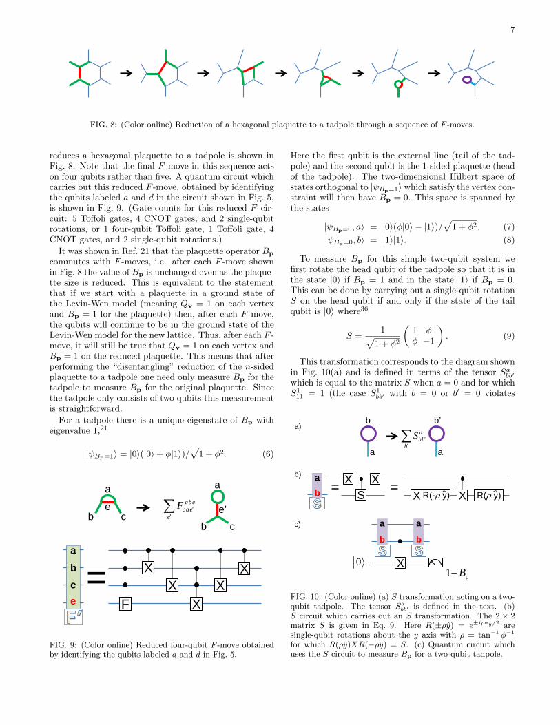
Here the first qubit is the external line (tail of the tad-pole) and the second qubit is the 1-sided plaquette (headof the tadpole). The two-dimensional Hilbert space ofstates orthogonal to |ψBp=1〉 which satisfy the vertex con-straint will then have Bp = 0. This space is spanned bythe states

|ψBp=0, a〉 = |0〉(φ|0〉 − |1〉)/√

1 + φ2, (7)

|ψBp=0, b〉 = |1〉|1〉. (8)

To measure Bp for this simple two-qubit system wefirst rotate the head qubit of the tadpole so that it is inthe state |0〉 if Bp = 1 and in the state |1〉 if Bp = 0.This can be done by carrying out a single-qubit rotationS on the head qubit if and only if the state of the tailqubit is |0〉 where36

S =1√

1 + φ2

(1 φφ −1

). (9)

This transformation corresponds to the diagram shownin Fig. 10(a) and is defined in terms of the tensor Sa

bb′

which is equal to the matrix S when a = 0 and for whichS111 = 1 (the case S1

bb′ with b = 0 or b′ = 0 violates

a

b

a

b’

∑′

′b

abbS

a)

c)

b)

= a b =

a

b

0p1 B−

a

b

S X X

X

X

R(-ρ y) X R(ρ y)

FIG. 10: (Color online) (a) S transformation acting on a two-qubit tadpole. The tensor Sabb′ is defined in the text. (b)S circuit which carries out an S transformation. The 2 × 2matrix S is given in Eq. 9. Here R(±ρy) = e±iρσy/2 aresingle-qubit rotations about the y axis with ρ = tan−1 φ−1

for which R(ρy)XR(−ρy) = S. (c) Quantum circuit whichuses the S circuit to measure Bp for a two-qubit tadpole.

8

0

3 4 5 6

1 2

9 10 11 12

7 8

b

a e c

d

b

e c

d a

a e

b

c a b

b

c

d

a

b

a e c

d

b

e c

d a

a e

b

c a b

b

e c

d

a

b

e c

d

a

p1 B−

6

1

2

4

3

12

9

10

11

7

8

5

p a

b

c

d

e e

X

FIG. 11: (Color online) Quantum circuit which can be used to measure Bp for the Fibonacci code on a hexagonal plaquettebased on the plaquette reduction shown in Fig. 8. It must be verified that Qv = 1 on each of the six vertices of the plaquettebefore carrying out the circuit.

the vertex constraint). A quantum circuit which carriesout this transformation (and its inverse since the circuitsquares to 1) is shown in Fig. 10(b). This circuit can becarried out with 1 CNOT gate and 2 single-qubit rota-tions. Like the F circuit, this simple construction is pos-sible because S2 = 1 and detS = −1. If the two tadpolequbits are initially in the state |ψBp=1〉 the result of car-rying out this circuit is the state |0〉|0〉. If the two tadpolequbits are initially in the two-dimensional Hilbert spacespanned by the states {|ψBp=0, a〉, |ψBp=0, b〉} then aftercarrying out this circuit they will be in the space spannedby the states {|0〉|1〉, |1〉|1〉}. In either case the state ofthe second qubit, i.e. the rotated head of the tadpole,will be equal to 1−Bp.

After carrying out the S circuit on the tadpole, aCNOT gate can be done with the head qubit as the con-trol qubit and a syndrome qubit, initialized to the state|0〉, as the target qubit. The syndrome qubit can thenbe measured and if the result is 0 then Bp = 1 for thetadpole (and hence for the original plaquette), and if theresult is 1 then Bp = 0.

After measuring Bp for the tadpole, the final step isto reconstruct the full plaquette. This can be done byundoing the S circuit on the tadpole and then undoingthe F -moves. Putting everything together the resultingmeasurement circuit for the case of a hexagonal plaquetteis the palindromic circuit shown in Fig. 11. In this circuitthe notation is the same as in the pentagon circuit, witheach box corresponding to either the full or reduced Fcircuit, or the S circuit, and the letters labeling the var-ious “inputs” as defined in Figs. 5,9, and 10. From thestructure of the circuit it is clear how this constructiongeneralizes to the case of an arbitrary n-sided plaquette.

We again emphasize that the circuit shown in Fig. 11only measures Bp correctly if the vertex constraint Qv =1 is satisfied on each vertex of the initial plaquette at thestart of the circuit. If the vertex constraint is violated onany of these vertices then by definition Bp = 0 for theplaquette;15 but the circuit will, in some cases, give thewrong result of Bp = 1. To see this, consider the actionof this circuit on the full 22n-dimensional Hilbert spaceof the 2n qubits associated with an n-sided plaquette, in-cluding those states which violate the vertex constraint.From the structure of the circuit, which performs a uni-tary transformation on 2n qubits and then measures thestate of a single qubit to determine Bp, it is clear that thedimensionalities of the Hilbert spaces for which Bp = 1or Bp = 0 would both be 22n−1, i.e. half that of thefull Hilbert space. However, once the vertex constraint istaken into account the Hilbert space is greatly reduced.The dimensionalities of the projected Hilbert spaces forwhich Qv = 1 on each of the n vertices and Bp = 1 orBp = 0 for the plaquette are Dim[Bp = 1] = F2n−1 andDim[Bp = 0] = F2n+1, respectively, where Fn is the nthFibonacci number (F0 = 0, F1 = 1, F2 = 1, F3 = 2,etc.). For the case of a hexagonal plaquette this meansthe full 4096 = 212 dimensional Hilbert space of twelvequbits is projected down to a space of dimensionality322 = F11 +F13 = 89+233 with an 89 dimensional spaceof states satisfying the plaquette constraint with Bp = 1.The reader will be reassured to know we have numeri-cally checked that the circuit shown in Fig. 11 performsthe correct measurement of Bp on this projected space.

It should be noted that the requirement that Qv = 1on each vertex before measuring Bp may cause prob-lems when extracting error syndromes. For example, if a

9

1 2 3

4

1 2 1 2 4 3

4

3

Initialize to Bp = a

Measure to find Bp = a

b

a

c e

b a

b

e

c a

a b =

SWA

P

1

2

3

4

a) b)

U

}4,4,3{},3,2,1{1+=vQ

FIG. 12: (Color online) (a) Sequence of F -moves which pulls a tadpole through a line. (b) Four-qubit quantum circuit whichinitializes a tadpole with an S circuit, carries out the sequence of two F -moves shown in (a), and then performs another Scircuit so that measuring qubit 3 would yield Bp for the new tadpole. The tadpole is initialized to a state with Bp = 1 or0 depending on whether the initial state of qubit 4 is |0〉 or |1〉, respectively. The circuit equality holds provided Qv = 1 onthe vertices of the initial lattice. As in Fig. 6(b) these vertices are labeled inside the red box. The 2× 2 matrix U is given byEq. 10 in the text.

faulty measurement of Qv gives 1 for a particular vertexon a plaquette, but the actual value of Qv is 0 for thatvertex, then, as described above, the Bp measurementcircuit for the plaquette will, in some cases, give Bp = 1even though the correct value (as it is for any plaquettein which a vertex constraint is violated) is Bp = 0. Inthis paper we have not addressed the important questionof whether it is possible to extract error syndromes forthe Fibonacci code fault tolerantly, nor the question ofprecisely how these errors would be corrected. Our goalhas been to construct circuits which, in the absence oferrors, can be used to measure Qv and Bp in order tobegin to get a measure of their complexity.

We can now give our final gate counts for measuringBp. If we choose to reduce all n-qubit Toffoli gates toconventional three-qubit Toffoli gates (using 4n−12 Tof-foli gates, following Ref. 28 as described in Sec. III) thenwe find that our procedure for an n-sided plaquette (withn ≥ 2) requires 18n−26 Toffoli gates, 8n−5 CNOT gatesand 4n single-qubit rotations. Alternatively, if we con-sider n-qubit Toffoli gates as primitives, then our proce-dure requires 2n− 4 five-qubit Toffoli gates, 2 four-qubitToffoli gates, 2n − 2 Toffoli gates, 8n − 5 CNOT gatesand 4n single-qubit rotations.37 Not surprisingly, this issignificantly more demanding than the analogous require-ment for the Kitaev surface code, for which only n CNOTgates are needed to measure the plaquette operator foran n-sided plaquette.

Finally we note that there are, of course, many differ-ent ways to reduce a given plaquette to a tadpole usingF -moves, all of which can be used to measure Bp andsome of which will be more “parallelizable” than others.

VII. A SIMPLE EXAMPLE

One of the motivations of the present work is to findsimple quantum circuits which might feasibly be carriedout in the near term and which begin to test some of the

key properties of the Fibonacci code. We have alreadyseen one example of such a circuit, the sequence of fivecontrolled-F gates which results in a two-qubit SWAPgate discussed in Sec. V. This circuit is a simplified ver-sion of the full seven-qubit pentagon circuit shown inFig. 6(b) and can potentially be used to calibrate the Foperation. In this section we give a similar example — afour-qubit circuit which first initializes a tadpole into astate with either Bp = 1 or 0, and then pulls this tadpolethrough a line using F -moves to produce a new tadpolewhich can be measured to verify that the value of Bp hasnot changed. As for the pentagon circuit, this four-qubitcircuit can be simplified to a two-qubit circuit which, inthis case, can be used to calibrate the S operation.

The sequence of operations we consider is illustrated inFig. 12(a). The system consists of a four-edged trivalentlattice and so uses four qubits, labeled 1 through 4 inthe figure. Initially two qubits (1 and 2) are assignedto edges which form a line and the other two qubits (3and 4) form a tadpole attached to this line. As always,in what follows we assume that it has been verified thatQv = 1 on each of the two vertices of this lattice at thestart of the process.

The first step is to initialize the tadpole in a state witheither Bp = 1 or 0. Then, using two F -moves, as shownin Fig. 12(a), the tadpole can be pulled through the line.The F -moves preserve Bp, and so the intermediate stateof this process is a 2-sided plaquette which has been ini-tialized either into the code space if Bp = 1 or outsideof the code space if Bp = 0. After the tadpole has beenpulled through the line, the two qubits forming the initialtadpole have swapped places — the head of the tadpoleis now the tail and vice versa. If Bp is now measured forthe new tadpole the result should yield the same value ofBp that the tadpole was initialized to at the start of theprocess.

The left-hand side of the circuit identity shown in Fig-ure 12(b) is a four-qubit circuit which carries out theprocedure described above. If qubit 4 is initially in the

10

=

=

a)

b)

SWA

P SW

AP

U X

X

XUX

FX S S XF

FX S S XF

FIG. 13: (Color online) (a) Simplified two-qubit circuit iden-tity obtained by setting qubits 1 and 2 to the state |1〉 in thecircuit identity shown in Fig. 12(b). (b) Equivalent circuitidentity obtained by moving the two NOT gates from the leftside of the identity shown in (a) to the right side.

state |1 − a〉 then the first S circuit initializes the tad-pole in a state with Bp = a. A reduced F circuit thencarries out the first F -move and produces a 2-sided pla-quette with Bp = a. Next, a second reduced F circuitcarries out the second F -move producing a new tadpolewith Bp = a but with the head and tail of the tadpoleinterchanged. Finally, after carrying out an S circuit onthis tadpole the state of qubit 3 will be |1− a〉.

Note that if qubit 4 is initially in the state |1〉 so thatthe tadpole is initialized to a state with Bp = 0 thenqubit 3 can initially be in either the state |0〉 or |1〉 whilestill satisfying the vertex constraint. After the first S cir-cuit on the left-hand side of Fig. 12(b) is carried out thetadpole will then be placed in a quantum superpositionof |ψBp=0, a〉 and |ψBp=0, b〉 (See Eqns. (7) and (8)). Atthe end of the circuit, after being pulled through the lineformed by qubits 1 and 2, the tadpole will still be in thetwo-dimensional Bp = 0 Hilbert space, but the particularsuperposition will in general have changed. Direct calcu-lation shows that if qubits 1 and 2 are both in the state |1〉then the operation acting on the two-dimensional Bp = 0space when pulling the tadpole through the line is givenby

U =

(−φ−2

√1− φ−4√

1− φ−4 φ−2

). (10)

Otherwise, if either qubit 1 or qubit 2 (or both) are inthe state |0〉 the state of the final tadpole will be thesame as that of the initial tadpole with the head and tailqubits swapped. These cases are all accounted for by theSWAP gate and four-qubit controlled-U operation on theright-hand side of the circuit identity in Fig. 12(b). Asfor the pentagon circuit, this identity only holds whenQv = 1 on the two vertices of the initial lattice (againthese vertices are labeled inside the red box in the figure).

This four-qubit circuit, which essentially represents ini-tializing a 2-sided plaquette into a state with a givenvalue of Bp and then producing a state which can bemeasured to determine Bp after carrying out a differentF -move than the one used to initialize it, is much sim-pler than the full circuit for measuring Bp for a hexagonal

plaquette. However, it still involves the four-qubit Toffoligate which appear in the reduced F circuit. As for thepentagon circuit, a simpler two-qubit circuit identity canbe found by fixing the states of the qubits which act effec-tively as control qubits (qubits 1 and 2 in Fig. 12). If wefix these qubits to both be in the state |1〉 we obtain thesimplified two-qubit circuit identity shown in Fig. 13(a).

This circuit identity can be simplified further by mul-tiplying both sides on the left and right by NOT gateswhich act on the top and bottom qubits, respectively, toobtain the equivalent circuit identity shown in Fig. 13(b).Note that if the initial state for the circuit shown inFig. 13(a) is |1〉|0〉, where the first qubit is the top qubit(qubit 3 in Fig. 12), then the vertex constraint is notsatisfied for the full four-qubit circuit. However, the sim-plified circuit identity is readily seen to be satisfied in thiscase. For all other cases the vertex constraint is satisfied,and so it follows that the expression shown in Fig. 13(a)and the equivalent expression in Fig. 13(b) are exact cir-cuit identities, independent of whether or not the vertexconstraint is satisfied.

The key action of the two-qubit circuit on the left-handside of Fig. 13(b) occurs when the tadpole is initializedin a state with Bp = 1 for which the tail qubit muststart in the state |0〉. For this case, after pulling thetadpole through the line the new tadpole must again bein the state with Bp = 1. Thus, after accounting for theremoval of the two NOT gates, this circuit must take thestate |1〉|0〉 to the state |0〉|1〉.

Like the five controlled-F SWAP circuit in Fig. 7,which can be used to calibrate the F matrix, the circuitidentity shown in Fig. 13(b) can be used to calibrate theS matrix. Once F has been fixed by the pentagon circuit,the requirement that the circuit on the left-hand side ofFig. 13(b) takes the state |1〉|0〉 to the state |0〉|1〉 fixesthe form of the matrix S (up to an overall phase which isirrelevant for our purposes). Note that in performing thiscalibration it is not necessary to carry out a full quan-tum process tomography. It is sufficient to verify thatthe circuit identity holds for the initial state |1〉|0〉. Forthis case, only the SWAP gate on the right-hand side isrelevant since the controlled-XUX gate enters only whenthe initial state of the second qubit is |1〉.

VIII. CONCLUSIONS

In this paper we have constructed explicit quantum cir-cuits for measuring the vertex and plaquette operators,Qv and Bp, in the Fibonacci Levin-Wen model. Theseoperators can be viewed as stabilizers for the Fibonaccicode,13 a surface code for which defects can behave as Fi-bonacci anyons — the simplest non-Abelian anyons forwhich braiding alone is universal for quantum compu-tation. While the Qv measurement is not significantlymore difficult than the analogous measurement for theKitaev surface codes (for which the defects behave asAbelian anyons), the Bp measurement scheme we present

11

here is significantly more difficult than its Abelian coun-terpart. While the present scheme is almost certainlynot the most efficient one for performing this measure-ment, given the complexity of the operator Bp it is likelythat even the most efficient schemes will require a largenumber of primitive gate operations. This cost in circuitcomplexity will then need to be weighed against the gainof not requiring magic state distillation. The situationis somewhat analogous to comparing the relative mer-its of performing topological quantum computation withIsing anyons (which requires magic state distillation) toFibonacci anyons.38

It is clear that further work will be needed before sucha direct comparison of the resources needed to carry outfault-tolerant quantum computation using the Fibonaccicode with that using the Kitaev surface code will bepossible. While recent progress strongly suggests thatthe Kitaev surface code is the most promising from thepractical point of view of trying to build an actual fault-tolerant quantum computer, we believe it is too early torule out the possibility that the Fibonacci code may havesome practical implications. Even if it does not, we be-lieve the Fibonacci code is of intrinsic interest, in partbecause computing with it can be viewed as essentiallysimulating a non-Abelian state of matter on a quantumcomputer.

Our measurement circuit for Bp is built out of circuitswhich realize F -moves and the action of the S matrixon a trivalent lattice. In addition to our measurementcircuits we have also given simpler circuits built out ofthese F and S circuits. The first is a seven-qubit circuit

which can be used to verify that the F circuit satisfies thepentagon equation, as well as a simpler two-qubit circuitwhich contains the nontrivial content of this equation andfixes the form of the F matrix. The second is a four-qubitcircuit which uses the S circuit to initialize a tadpole (1-sided plaquette) in a state with either Bp = 1 or 0, carriesout a sequence of F -moves to pull the tadpole through aline, and then produces a state which can be measuredto determine Bp for the new tadpole. For this circuit wehave also given a simpler two-qubit circuit which, onceF has been fixed by the pentagon circuit, fixes the formof the S matrix. These simple two-qubit circuits (Figs. 7and 13) may be useful for calibrating the F and S oper-ations.

A recurring theme in this work has been the need forn-qubit Toffoli gates (with n = 3, 4 and 5) when com-puting with the Fibonacci code. These n-qubit Toffoligates arise as a natural consequence of the non-Abeliannature of this code. We believe the possibility of usingnon-Abelian surface codes such as the Fibonacci codefor fault-tolerant quantum computation provides furthermotivation for developing experimental techniques to di-rectly carry out accurate n-qubit Toffoli-class gates.

Acknowledgments

NEB acknowledges support from US DOE Grant No.DE-FG02-97ER45639 and DDV is grateful for supportfrom the Alexander von Humboldt foundation.

1 A. Kitaev, Ann. Phys. 303, 2 (2003).2 S. B. Bravyi and A. Y. Kitaev, arXiv: quant-ph/9811052.3 R. Raussendorf and J. Harrington, Phys. Rev. Lett. 98,

190504 (2007).4 R. Raussendorf, J. Harrington, and K. Goyal, New J. Phys.9, 199 (2007).

5 A. G. Fowler, A. M. Stephens, and P. Groszkowski, Phys.Rev. A 80, 052312 (2009).

6 S. Bravyi and A. Kitaev, Phys. Rev. A 71, 022316 (2005).7 H. Bombin and M. A. Martin-Delgado, Phys. Rev. Lett.97, 180501 (2006).

8 H. Bombin and M. A. Martin-Delgado, Phys. Rev. Lett.98, 160502 (2007).

9 H. Bombin, New J. Phys. 13, 043005 (2011).10 A. G. Fowler, Phys. Rev. A 83, 042310 (2011).11 A. J. Landahl, J. T. Anderson, and P. R. Rice,

arXiv:1108.5738.12 D. S. Wang, A. G. Fowler, and L. C. L. Hollenberg, Phys.

Rev. A 83, 020302 (2011).13 R. Konig, G. Kuperberg, and B. W. Reichardt, Ann. of

Phys. 325, 2707 (2010).14 V. G. Turaev and O. Y. Viro, Topology 31, 865 (1992).15 M. A. Levin and X.-G. Wen, Phys. Rev. B 71, 045110

(2005).16 The connection between the Turaev-Viro invariants and

the Levin-Wen models is discussed in Sec. 7 of Ref. 13. Seealso Z. Kadar, A. Marzuoli, M. Rasetti, Int. J. QuantumInform. 7 195 (2009); and F. J. Burnell and S. H. Simon,Ann. of Phys. 325, 11, 2550 (2010).

17 M. Freedman, M. Larsen, and Z. Wang, Commun. Math.Phys. 227, 605 (2002).

18 N. E. Bonesteel, L. Hormozi, G. Zikos, and S. H. Simon,Phys. Rev. Lett. 95, 140503 (2005).

19 L. Hormozi, G. Zikos, N. E. Bonesteel, and S. H. Simon,Phys. Rev. B 75, 165310 (2007).

20 E. Dennis, A. Kitaev, A. Landahl, and J. Preskill, J. Math.Phys. (N.Y.) 43, 4452 (2002).

21 R. Konig, B. W. Reichardt, and G. Vidal, Phys. Rev. B79, 195123 (2009).

22 D. P. DiVincenzo, Phys. Scr. T 137, 014020 (2009).23 B0

p is the identity operator when acting on states which sat-isfy the vertex constraint. Thus only B1

p contributes non-trivially to Bp for the Fibonacci code with the particularlinear combination (3) forming a projection operator (seeRef. 15).

24 M. Mariantoni, H. Wang, T. Yamamoto, M. Neeley, R.C. Bialczak, Y. Chen, M. Lenander, E. Lucero, A. D.O’Connell, D. Sank, M. Weides, J. Wenner, Y. Yin, J.Zhao, A. N. Korotkov, A. N. Cleland, and J. M. Martinis,Science 334, 61 (2011).

12

25 A. Fedorov, L. Steffen, M. Baur, M. P. da Silva, and A.Wallraff, Nature 481, 170 (2012).

26 M. D. Reed, L. DiCarlo, S. E. Nigg, L. Sun, L. Frunzio, S.M. Girvin, and R. J. Schoelkopf, Nature 482, 382 (2012).

27 T. Monz, K. Kim, W. Hansel, M. Riebe, A. S. Villar, P.Schindler, M. Chwalla, M. Hennrich, and R. Blatt, Phys.Rev. Lett. 102, 040501 (2009).

28 A. Barenco, C. H. Bennett, R. Cleve, D. P. DiVincenzo,N. Margolus, P. Shor, T. Sleator, J. A. Smolin, and H.Weinfurter, Phys. Rev. A 52, 3457 (1995).

29 J. I. Cirac and P. Zoller, Phys. Rev. Lett. 74, 4091 (1995).30 X.-M. Lin, Z.-W. Zhou, M.-Y. Ye, Y.-F. Xiao, and G.-C.

Guo, Phys. Rev. A 73, 012323 (2006).31 L.-M. Duan, B. Wang, and H. J. Kimble, Phys. Rev. A 72,

032333 (2005).32 T. C. Ralph, K. J. Resch, and A. Gilchrist, Phys. Rev. A

75, 022313 (2007).33 n-qubit Toffoli gates can be carried out efficiently (for

n = 3 − 8) using 2n − 2 CNOT gates and 2n single-qubitrotations (see Ref. 28). Thus our Qv measurement circuit(Fig. 2) can be carried out using 17 CNOT gates and 16single-qubit rotations.

34 R. P. Feynman, Opt. News 11, 11 (1985).35 A. Barenco, D. Deutsch, A. Ekert, and R. Jozsa, Phys.

Rev. Lett. 74, 4083 (1995).36 S is the so-called modular S matrix for Fibonacci anyons.37 If all n-qubit Toffoli gates are simulated using CNOT gates

and single qubit rotations following Ref. 28, (see Ref. 33)we find the total gate count for measuring Bp for an n-sided plaquette with n ≥ 2 is 80n− 109 CNOT gates and84n−112 single-qubit rotations. This gate count should beviewed as an upper bound because we have not consideredpossible gate merging.

38 M. Baraban, N. E. Bonesteel, and S. H. Simon, Phys. Rev.A 81, 062317 (2010).