Quantum chemistry in parallel with PQS

Software News and Update

Quantum Chemistry in Parallel with PQS

JON BAKER,1,2 KRZYSZTOF WOLINSKI,1,3 MASSIMO MALAGOLI,1 DON KINGHORN,1

PAWEL WOLINSKI,1 GABOR MAGYARFALVI,4 SVEIN SAEBO,5 TOMASZ JANOWSKI,2 PETER PULAY1,2

1Parallel Quantum Solutions, 2013 Green Acres Road, Suite A, Fayetteville, Arkansas 727032Department of Chemistry, University of Arkansas, Fayetteville, Arkansas 727013Department of Chemistry, Maria Curie-Sklodowska University, Lublin, Poland

4Institute of Chemistry, Eotvos Lorand University, H-1518 Budapest 112, Pf. 32, Hungary5Department of Chemistry, Mississippi State University, Mississippi State, Mississippi 39762

Received 18 February 2008; Accepted 9 May 2008DOI 10.1002/jcc.21052

Published online 9 July 2008 in Wiley InterScience (www.interscience.wiley.com).

Abstract: This article describes the capabilities and performance of the latest release (version 4.0) of the Parallel

Quantum Solutions (PQS) ab initio program package. The program was first released in 1998 and evolved from the

TEXAS program package developed by Pulay and coworkers in the late 1970s. PQS was designed from the start to

run on Linux-based clusters (which at the time were just becoming popular) with all major functionality being (a)

fully parallel; and (b) capable of carrying out calculations on large—by ab initio standards—molecules, our initial

aim being at least 100 atoms and 1000 basis functions with only modest memory requirements. With modern hard-

ware and recent algorithmic developments, full accuracy, high-level calculations (DFT, MP2, CI, and Coupled-Clus-

ter) can be performed on systems with up to several thousand basis functions on small (4-32 node) Linux clusters.

We have also developed a graphical user interface with a model builder, job input preparation, parallel job submis-

sion, and post-job visualization and display.

q 2008 Wiley Periodicals, Inc. J Comput Chem 30: 317–335, 2009

Key words: parallel computing; ab initio; density functional theory; high-level post-HF methods; graphical user

interface

Introduction

This article documents and describes the capabilities of the Par-

allel Quantum Solutions (PQS) ab initio program package. PQS1

was formed in 1997 with the aim of providing a combined per-

sonal computer-based hardware/software platform, which would

make available the most commonly used ab initio methods, fully

parallel, at a greatly increased performance/price ratio when

compared with the workstations and mainframes then available.

By 1997, the performance of personal computers (PCs) was

approaching that of much more expensive workstations at a frac-

tion of the cost, and it became obvious to us (and others) that

clusters of PCs running the stable and freely available Linux

operating system were going to be a tremendous new resource

for computational chemists.

The origins of what was to develop into the PQS program go

back to the late 1960s when Meyer and Pulay began writing a

new ab initio program at the Max-Planck Institute for Physics and

Astrophysics in Munich. The primary purpose of this project was

to implement new ab initio techniques. At this time, Meyer was

interested in highly accurate correlation methods such as pseudo-

natural orbital-configuration interaction (PNO-CI),2 the coupled-

electron pair approximation (CEPA),3 and spin density calcula-

tions. Pulay wanted to implement analytical energy derivatives

(forces), gradient geometry optimization, and force constant calcu-

lations via the numerical differentiation of analytical forces.4 At

first, analytical gradients were restricted to closed-shell Hartree-

Fock wavefunctions, but in 1970, they were generalized to unre-

stricted (UHF) and restricted open-shell (ROHF) methods.5 The

first version of the code was completed in early 1969, simultane-

ously at the Max-Planck Institute and the University of Stuttgart.

It was named MOLPRO by Meyer and used Gaussian lobe func-

tions, primarily at the behest of Preuss, the group leader in Munich

and the inventor of Gaussian lobe basis sets.6

In the 1970s, Werner and Reinsch, working with Meyer,

added a number of advanced methods to MOLPRO, for instance

multiconfiguration self-consistent field (MC-SCF)7 and internally

contracted multireference configuration interaction (MR-CI).8,9

The current MOLPRO package, although derived from this code,

Correspondence to: J. Baker; e-mail: [email protected]

q 2008 Wiley Periodicals, Inc.

has been largely rewritten and much extended by Werner, Knowles

and coworkers starting in the 1980s and continuing today.10

Meanwhile Pulay, visiting Boggs at the University of Texas,

Austin and Schaefer at the University of California, Berkeley in

1976, wrote a new program, also based on the original MOL-

PRO, that replaced Gaussian lobes with the more efficient stand-

ard Gaussians. This program, finished at Austin, was called

TEXAS. It emphasized large (by the standards of the 1970s)

molecules, SCF convergence,11 geometry optimization techni-

ques,12 and vibrational spectroscopy-related calculations.13

TEXAS was further developed at the University of Arkansas

from 1982 onward. The first major addition was the implementa-

tion of several local electron correlation methods by Saebo14

and a first-order MC-SCF program by Hamilton. A significant

addition was the implementation of the first practical gauge-

invariant atomic orbital (GIAO) NMR chemical shift program15

by Wolinski, who also added a highly efficient integral package.

Bofill implemented an unrestricted natural orbital-complete

active space (UNO-CAS) program including analytical gra-

dients16; this is a low-cost alternative to MC-SCF and works

just as well in most cases. TEXAS was first parallelized in

1995–1996 on a cluster of 10 IBM RS6000 workstations.

In 1996, Baker joined the Pulay research group and, in the

same year, Intel brought out the Pentium Pro. For the first time, a

PC existed that was competitive with low-end workstations and

less expensive by about an order of magnitude. Realizing the

potential of this development for computational chemistry, PQS

was formed and an SBIR grant application was submitted in July

1997 for the commercial development of PC clusters for parallel

ab initio calculations. Meanwhile, the Pulay group, funded by a

National Science Foundation grant, set about constructing a Linux

cluster using 300 MHz Pentium II processors. By a fortunate cir-

cumstance, several highly talented and computer literate graduate

students were in the group at that time, in particular Magyarfalvi

and Shirel. The PC cluster was a complete success, and signifi-

cantly outperformed the IBM Workstation cluster that was the

group’s computational mainstay at a fraction of its cost.

The PQS software was loosely modeled on the TEXAS code

and parts of it (principally the NMR code) were licensed to PQS

from the University of Arkansas. However, much of the code was

extensively rewritten to conform to our twin aims of (a) having all

major functionality fully parallel; and (b) being able to routinely

perform calculations on large systems (Initially, in the late 1990s,

we took to this to mean at least 100 atoms and at least 1000 basis

functions; it is a measure of how far the field has developed since

then that systems of this size are now only regarded as modest).

We have always aimed primarily for a modest level of parallelism

(from 8 to 32 CPUs), as this is the most common size for an indi-

vidual or group resource. Even on very large clusters it is unusual

for any given user to be allocated more than a percentage of the

available processors, and so our target level of parallelism is still

generally applicable regardless of the actual cluster size.

The current capabilities of the PQS program, most of which

were added after 1998, are as follows:

� An efficient vectorized Gaussian integral package allowing

high-angular momentum basis functions and general contrac-

tions.

� Abelian point group symmetry throughout; utilizes full point

group symmetry (up to Ih) for geometry optimization step and

solution of the coupled-perturbed HF equations for analytical

Hessian (second derivative) calculations.

� Closed-shell (RHF) and open-shell (UHF) SCF energies and

gradients, including several initial wavefunction guess options.

Improved SCF convergence for open-shell systems.

� Closed-shell (RHF) and open-shell (UHF) density functional

energies and gradients including all popular exchange-

correlation functionals: VWN local correlation, Becke 88 non-

local exchange, Lee-Yang-Parr nonlocal correlation, B3LYP,

etc.

� Fast and accurate ‘‘pure’’ (i.e., nonhybrid) DFT energies and

gradients for large systems and large basis sets using the Fou-

rier transform coulomb (FTC) method.

� Efficient, flexible geometry optimization for all these methods

including Baker’s Eigenvector following (EF) algorithm for

minimization and saddle-point search, Pulay’s GDIIS algo-

rithm for minimization, use of Cartesian, Z-matrix, and delo-

calized internal coordinates. Includes new coordinates for effi-

cient optimization of molecular clusters and adsorption/reac-

tion on model surfaces.

� Full range of geometrical constraints including fixed distances,

planar bends, torsions, and out-of-plane bends between any

atoms in the molecule and frozen (fixed) atoms. Atoms

involved in constraints do not need to be formally bonded

and—unlike with a Z matrix—desired constraints do not need

to be satisfied in the starting geometry. We have recently

added composite constraints (linear combinations of individual

constraints).

� Analytical (and numerical) second derivatives for all these

methods, including the calculation of vibrational frequencies,

IR/Raman intensities, vibrational circular dichroism (VCD)

rotational strengths, and thermodynamic analysis.

� Scaled quantum mechanical (SQM) force field for fitting to

experimental vibrational spectra. Scale factors can be opti-

mized for best fits to a given set of experimental fundamen-

tals. Precalculated scale factors (for H, C, N, O, and Cl) give

better agreement with experiment for both vibrational frequen-

cies and IR intensities.

� Nuclear magnetic resonance shielding tensors using GIAO

(Gauge Including Atomic Orbital) or London basis sets for

RHF and DFT wavefunctions.

� A full range of effective core potentials (ECPs), both relativis-

tic and nonrelativistic, with energies, gradients, analytical sec-

ond derivatives, and NMR.

� Closed-shell MP2 energies and analytical gradients and dual-

basis MP2 energies; numerical MP2 second derivatives.

� High level post-HF closed-shell energies for several methods

including configuration interaction singles and doubles (CID,

CISD), quadratic CI singles and doubles (QCISD), CEPA-0

and CEPA-2; coupled-cluster singles and doubles (CCD,

CCSD) with perturbative triples (CCSD(T)) and MP3 and

MP4

� Potential scan, including scan 1 optimization of all other

degrees of freedom.

� Reaction path (IRC) following using either Z-matrix, Carte-

sian, or mass-weighted Cartesian coordinates.

318 Baker et al. • Vol. 30, No. 2 • Journal of Computational Chemistry

Journal of Computational Chemistry DOI 10.1002/jcc

� Conductor-like screening solvation model (COSMO) including

energies, analytical gradients, numerical second derivatives,

and NMR.

� Population analysis, including bond orders and atomic valen-

cies (with free valencies for open-shell systems); CHELP

(charge from electrostatic potential), and Cioslowski charges.

� Weinhold’s natural bond order (NBO) analysis, including nat-

ural population and steric analysis.

� Properties module with charge, spin-density, and electric field

gradient at the nucleus.

� Polarizabilities, hyperpolarizabilities, and dipole and polariz-

ability derivatives.

� Full Semiempirical package, both open (unrestricted) and

closed-shell energies and gradients, including MINDO/3,

MNDO, AM1, and PM3 For the latter, all main group ele-

ments through the fourth row (except the noble gases) as well

as zinc and cadmium have been parametrized.

� Molecular mechanics using the Sybyl 5.2 and UFF force

fields.

� QM/MM using the ONIOM method.

� Molecular dynamics using the Verlet algorithm.

� Pople-style input for quick input generation and compatibility

with other programs.

We do not propose to discuss any of the capabilities listed

in detail here. Many of them are by now standard and are

available in a number of different quantum mechanical pack-

ages. In what follows we emphasize parallelism, those techni-

ques that are unique to PQS, or particular algorithms that we

have developed that, for example, allow methods that have in

the past been applicable to small molecules only to be

extended to much larger molecules and basis sets, such as our

post-Hartree-Fock capabilities.

Parallelism

This has been of fundamental importance since the beginning of

PQS. As befits our focus on Linux clusters, our primary parallel

paradigm is message-passing. There are two basic toolkits for

message-passing parallelism: parallel virtual machine (PVM)17

and message passing interface (MPI).18 They are similar both in

concept and in their actual command structure and it is fairly

straightforward to convert a PVM program to MPI and viceversa. Indeed, we have recently developed an interface that

allows uniform access to either PVM or MPI commands from

the same call, and we can compile and link PVM or MPI ver-

sions of PQS from a single set of source files.

MPI is more widely used than PVM. The main difference

between them is that PVM includes an actual implementation,

whereas MPI is a set of standards allowing for different imple-

mentations. This feature is both an advantage and a disadvant-

age. It facilitates the adaptation of the code for newer hardware

architectures; several hardware vendors provide customized MPI

libraries that can take advantage of modern, high-speed, low-la-

tency networks such as Infiniband or Myrinet. PQS can use

these libraries with its MPI version, whereas PVM has to rely

on the network infrastructure available through the operating

system (the latter has improved significantly in recent years, and

gigabit Ethernet is now widespread). However, the reasonably

high computation/communication ratio of most quantum

chemistry tasks keeps the more easily deployed PVM version

competitive.

On the other hand, there can be subtle differences between

various implementations of MPI—of which there are several—

causing potential incompatibilities. The development of PVM

has been essentially confined to one group at Oak Ridge

National Laboratory, and both the library of calls and the pro-

gramming interface have stabilized since the mid 1990s.

Until recently our primary parallel development platform has

been PVM as when we first tested the versions of PVM and

MPI available to us back in 1998, we found that the PVM ver-

sion ran somewhat faster. Furthermore, our initial parallel MP2

energy algorithm (discussed later) spawns an additional slave

process on each node during the second integral half-transforma-

tion, and this spawning was far easier to accomplish using PVM

than with MPI (in fact for many years, the ability to spawn addi-

tional processes at all using MPI was not available until the

MPI-2 standard was accepted and implemented).

In our simple master-slave implementation, one process (or

CPU) is designated as the master process and is responsible for

assigning tasks to the other (slave) processes. All residual serial

(nonparallel) code is executed by the master process. Parallelism

is best achieved with the least possible transfer of data between

the various processes; ideally, at the start of the job, a single

number (e.g., a given atom) is sent from the master to the

slaves, which subsequently do all of the actual number crunch-

ing, passing the final data back to the master at the end of the

calculation for accumulation and print out. Although this ideal is

rarely achieved in actual practice, the basic features are at the

heart of all efficient parallel code: (1) Keep the amount of data

transferred to a minimum; and (2) reduce the residual serial

code to a minimum. In most cases, the node running the master

process also runs a slave process, as in an efficient parallel code,

the master process does as little as possible and all of the CPU

cycles ought to be available for use by the slave process. The

effect of residual serial code diminishes parallel efficiency more

than simple intuition suggests. For instance, 95% parallel effi-

ciency sounds impressive until one realizes that the 5% serial

overhead limits the speedup on 16 CPUs to a factor of just over

9, only 57% of the theoretical maximum.

Before discussing some of our own implementations in PQS,

we note that parallelism is of increasing importance in computa-

tional chemistry and is particularly so at the current time. As

mentioned in the Introduction section, the first parallel cluster

that we constructed in 1998 used 300 MHz Pentium II process-

ors. Since that time, processor speed (in addition to cache size

and other features) has been continually improving, and 3.0 GHz

and even higher rated processors are currently readily available.

Prior to the mid-1990s, and the onset of the PC revolution, par-

allel computers were very specialized, took several years to de-

velop, and often required major code rewrites to maximize per-

formance on the particular hardware design. By the time such

machines were actually released onto the market, the perform-

ance of their processors had often been substantially superseded

by those of the latest single-processor workstations, significantly

319Quantum Chemistry and PQS


reducing the advantages of their parallel architecture. At the

moment however, it appears that traditional silicon technology

has hit a fundamental limit to the speed of a single processor,

and manufacturers are improving compute power not by making

each processor faster, but by putting more than one CPU in the

same physical unit. At the time of writing (2007), dual-core pro-

cessors (i.e., two CPUs in the same processor) have been avail-

able for about 2 years and quad-core processors have just been

released. Such processor design naturally implies parallelism if

one wants to get the best performance for a single job.

Hartree-Fock Self-Consistent Field Calculations

The basic task during a self-consistent field (SCF) energy calcu-

lation is computation of the two-electron repulsion integrals and

their contraction with the appropriate density matrix elements to

construct the Fock matrix at each iterative cycle of the SCF

(Hartree-Fock or DFT) procedure. There are a number of com-

putational tasks in ab initio quantum chemistry that involves a

similar contraction step, e.g., the calculation of analytical gra-

dients (forces) on the atoms, and so parallelization of Fock ma-

trix construction serves as a template for the parallelization of

several other, related, computational steps. We use a simple

replicated memory model in which local copies of the density

and Fock matrices are stored by each slave process. This

approach is open to criticism because it does not use the avail-

able aggregate memory efficiently and the system size limit (as

far as memory is concerned) is effectively the same on a single

node as it is on the entire cluster. In practice however, memory

capacity has increased so much in recent years that the real bot-

tleneck on moderately large clusters is computing time.

Although the standard mode in PQS is fully direct (i.e., two-

electron integrals are not stored but are recalculated every time

they are needed), we will describe its generalization, the semi-

direct algorithm, in which the most expensive integrals are pre-

computed and stored on disk.19

At the start of the calculation, integrals over shell quartets

are allocated a ‘‘cost’’ which depends on how expensive they are

to compute (in terms of estimated CPU time) and their magni-

tude. ‘‘High-cost’’ integrals are precomputed and written to disk.

We use a d-density approach in our SCF algorithm,20 and so

what really counts is the change in the density from the previous

cycle. If a particular density matrix element converges rapidly,

then integrals that contribute to that density matrix element, par-

ticularly if they are small in magnitude, will quite quickly cease

to contribute to the change in the Fock matrix, and can subse-

quently be neglected. Such integrals are considered as ‘‘low

cost’’ and are recomputed as needed. The threshold separating

high and low cost depends on the available disk storage, defined

in the input. The semidirect feature speeds up the calculation

initially, but storing too many integrals becomes increasingly

inefficient as the I/O time required to read them back becomes

prohibitive.

In our simple master-slave model, integral shell indices are

passed to each slave process, initially in batches of, e.g., 50 or

so at a time, finally as individual shell quartets to ensure good

load balance. Integrals are written to the local disk of the slave

node on which they are calculated. The indices are passed

initially in a round-robin, and then first come-first served; as

soon as a slave sends a message to the master node that it has

finished calculating its current batch of integrals, it is sent the

next batch and so on until all the ‘‘high-cost’’ integrals have

been computed and stored.

When all the ‘‘high-cost’’ integrals have been computed and

written to disk, the ‘‘direct’’ phase of the SCF starts. At the start

of a given SCF cycle (other than the first, when only the initial

guess density is available), the difference density matrix is con-

structed from the current density matrix and the density matrix

on the previous cycle, and its lower triangle is broadcast to all

slaves from the master process. Each slave process then com-

mences to construct its own local copy of the difference Fock

matrix (lower triangle). It first reads back and constructs the

appropriate Fock matrix contributions from those integrals that

have been stored locally on its own disk. Once this is complete,

the slave then requests new (from the previously uncomputed)

integral indices from the master, which are passed to whichever

slave asks for them, initially in batches, then decreasing in size

to individual shell quartets according to the guided self-schedul-

ing algorithm.21 As the SCF process converges, the difference

density tends to zero, and an increasing fraction of integrals

whose contribution, when multiplied by the appropriate differ-

ence density matrix elements, are below a given threshold (typi-

cally 10210) need not be computed. Estimates of the integral

values are obtained via the well-known Schwartz inequality.22

When all integrals have been processed, all local copies of the

Fock matrix on all slaves are accumulated on the master node

via a binary tree algorithm.

Once the Fock matrix on a given cycle has been constructed,

it has to be diagonalized (or its equivalent) to form new molecu-

lar orbitals, and hence a new density matrix for the next itera-

tion. There are also other matrix manipulations, e.g., for SCF

convergence acceleration, such as DIIS,11 level shifting,23 or

other related techniques. Currently, the majority of these proce-

dures are not parallel in our code, and consequently contribute

to the serial overhead. Despite this, especially for systems with

little or no useable symmetry, the parallel efficiency of our basic

SCF code is high—typically greater than 7.0 on 8 CPUs—for

systems with up to 2000 basis functions. Above this, the serial

overhead (particularly the diagonalization step) begins to have a

greater impact and reduces the parallel efficiency. We routinely

use pseudodiagonalization24 and only calculate a subset of the

Fock matrix eigenvalues and eigenvectors (those corresponding

to the occupied orbitals and the lowest virtual) on most SCF

cycles, which significantly reduces the CPU time (but does not

reduce the scaling of the serial overhead with system size). On

the final cycle, to maintain numerical accuracy, the Fock matrix

is formed using the full (not the difference) density, and a full

diagonalization is forced, which gives a complete set of orbitals,

both occupied and virtual.

The above is typical of the way we have parallelized most of

the integral-based tasks in the PQS code, for example, in SCF

energy gradients, analytical second derivatives, NMR chemical

shifts, etc. Integral shell indices are passed from master to slave,

and the actual integrals are computed and used on the slaves,

usually via local copies of intermediate or final quantities (for

example, local copies of the gradient vector over atoms for SCF



forces). The passing of just shell indices minimizes data transfer

and the first come-first served nature, in which the next batch of

indices is passed to whichever slave finishes its current task first,

ensures that the slaves are nearly always busy and helps main-

tain good load balance, even on inhomogeneous systems in

which the CPUs differ in processing speed.

Semidirect Versus Full-Direct

As indicated in the earlier description of our basic SCF proce-

dure, integrals can either be recomputed where necessary at each

SCF cycle or written to disk and reread. It is also possible to

store integrals directly in memory. The latter is becoming an

increasingly viable option as larger capacity memory modules

become available (along with more memory slots per mother-

board). The amount of RAM available per node will only

increase in the future, especially since the switch a few years

back to 64-bit architecture eliminated the previous practical limit

of 2 GB per CPU.

For many years (at least since the late 1970s), increases in

CPU speed has significantly outpaced corresponding improve-

ments in I/O performance; consequently memory access time is

currently many times faster than disk I/O. When data is written

to an external unit, it is initially written to an I/O buffer that

resides in physical memory. Only when the buffer is full is the

data actually written to external storage. Unless a limit is delib-

erately placed on either the size or the number of buffers to a

given I/O unit, modern Linux operating systems can effectively

extend the I/O buffer up to the limits of the remaining physical

memory. Only when the amount of data written exceeds the avail-

able memory is there any actual disk access. As long as this limit

is not exceeded, writing to disk is about the same performance-

wise as storing integrals directly in memory.

However, once the available physical memory is exceeded,

and real disk access is required, the performance suffers consid-

erably. Consequently, semidirect jobs that attempt to store large

numbers of integrals (i.e., that require real disk access) show

significant performance degradation when compared with the

same job run full-direct (with no integral storage). Our experi-

ence has been that if a significant percentage of the total number

of integrals can be stored (either in core or in the I/O buffer)

without exceeding the total physical memory available on the

system, then there can be a major reduction in the elapsed time

required to complete the SCF procedure. If, on the other hand,

this percentage is small, then there is little or no gain in running

semidirect. Once the storage requested for integrals exceeds the

available physical memory, semidirect jobs are almost always

slower than full-direct. This situation is unlikely to change

unless there are real improvements in I/O speed.

Density Functional Theory

Density functional theory (DFT) is now the most popular tech-

nique for including electron correlation and is a ‘‘must have’’ in

any package that claims to support the most commonly used

methods. PQS has a large range of exchange-correlation (XC)

functionals plus the ability for the user to define his or her own

functional via linear combinations of existing exchange and/or

correlation functionals. There is continuing development in this

area with several groups introducing new functionals on a fairly

regular basis. Unfortunately, the proliferation of new functionals

creates more problems than it solves, and is a step toward semi-

empirical theory. It also makes it difficult to keep the program

up-to-date. Although the authors of new functionals may dis-

agree, it seems fair to say that the newer functionals have not

significantly and consistently improved upon the major

exchange-correlation functionals developed in the late 1980s–

early 1990s, although they may offer improved performance in

specific situations, such as kinetics.25 Functionals such as

Becke’s 1988 nonlocal exchange,26 Lee, Yang, and Parr’s (LYP)

nonlocal correlation,27 Perdew and Wang’s 1991 exchange-cor-

relational functional,28 and, of course, hybrid functionals such as

B3LYP (note that Becke’s original hybrid functional was

actually B3PW91 in modern parlance)29 are still the most widely

used. One of the more recent functionals which has proven use-

ful in our opinion is Handy and Cohen’s optimized nonlocal

exchange (OPTX, 2001),30 and OLYP (the combination of

OPTX with LYP) has proven to be more accurate than the more

popular BLYP, at least for general organic chemistry.31

As is typical for authors who have a traditional quantum

chemistry background, our basic DFT implementation is a modi-

fication of our Hartree-Fock program in which the exchange op-

erator has been partly or fully replaced by the DFT exchange-

correlation operator. The Coulomb part of the Fock matrix is

calculated, as in standard Hartree-Fock theory, using two-elec-

tron repulsion integrals. The physical simplicity of the electro-

static interaction allows alternative methods of evaluating the

Coulomb interaction to be used that scale better with system

size and are more efficient. For the most part, these methods

offer significant advantages only for ‘‘pure’’ (non-hybrid) density

functionals, as the calculation of exact exchange requires the

evaluation of electron repulsion integrals. We will discuss a par-

ticularly efficient way of evaluating the Coulomb terms, the

Fourier transform coulomb (FTC) method, in a later section.

The present discussion is restricted to the traditional integral-

based DFT code.

The DFT contribution (to the SCF energy, the force, and the

Hessian) is determined separately from the Coulomb term and is

computed via numerical integration over spherical atom-centered

grids using techniques pioneered in this context by Becke.32 Our

own procedure has been described earlier,33,34 and involves an

outer loop over grid points and parallelization over atoms. This

has some limitations; for example, in small systems, the number

of processors that can readily be used is limited to the number of

symmetry-unique atoms, but this is rarely a problem in practical

applications and has the advantage of being very convenient to

code. Load balance, which could conceivably cause difficulties, is

typically very good, especially if contributions from the heavier

atoms are calculated first, and those from hydrogen atoms are

done last. Only in clusters of identical atoms which do not divide

well into the number of available CPUs does this become an

issue. In the traditional approach, the calculation of the exchange-

correlation terms is generally a relatively minor computational

task compared to the calculation and processing of the two-elec-

tron repulsion integrals. This is not necessarily true if alternative

techniques are used to evaluate the Coulomb terms.



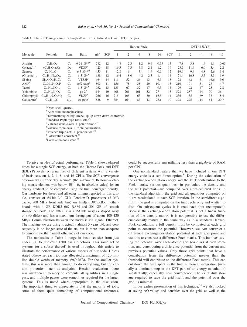
To give an idea of actual performance, Table 1 shows elapsed

times for a single SCF energy, at both the Hartree-Fock and DFT

(B3LYP) levels, on a number of different systems with a variety

of basis sets, on 1, 2, 4, 8, and 16 CPUs. The SCF convergence

criterion was sufficiently accurate (the maximum Brillouin-violat-

ing matrix element was below 1025 Eh in absolute value) for an

energy gradient to be computed using the final converged density.

Our hardware for these, and all other timings reported in this arti-

cle, consists of 64-bit 3.0 GHz Pentium-D processors (2 MB

cache, 800 MHz front side bus) on Intel(r) D955XBX mother-

boards with 4 GB DDR2 667 RAM and 304 GB of scratch

storage per node. The latter is in a RAID0 array (a striped array

of two disks) and has a maximum throughput of about 100–120

MB/s. Communication between the nodes is via gigabit Ethernet.

The machine we are using is actually almost 3 years old, and con-

sequently is no longer state-of-the-art, but is more than adequate

to demonstrate the parallel efficiency of our code.

The molecules in Table 1 range in basis set size from just

under 300 to just over 1500 basis functions. This same set of

systems (or a subset thereof) is used throughout this article to

illustrate the performance of various aspects of our code. Unless

stated otherwise, each job was allocated a maximum of 120 mil-

lion double words of memory (960 MB). For the smaller sys-

tems, this was more than enough to do everything, but for cer-

tain properties—such as analytical Hessian evaluation—there

was insufficient memory to compute all quantities in a single

pass, and multiple passes were sometimes required for the larger

systems. This is noted where appropriate in the discussion.

The important thing to appreciate is that the majority of jobs,

some of them quite demanding of computational resources,

could be successfully run utilizing less than a gigabyte of RAM

per CPU.

One nonstandard feature that we have included in our DFT

energy code is a semidirect option.34 During the calculation of

the exchange-correlation energy and the DFT contribution to the

Fock matrix, various quantities—in particular, the density and

the DFT potential—are computed over atom-centered grids. In

the standard algorithm, the grid and all quantities computed on

it are recalculated at each SCF iteration. In the semidirect algo-

rithm, the grid is computed on the first cycle only and written to

disk. On subsequent cycles it is read back (not recomputed).

Because the exchange-correlation potential is not a linear func-

tion of the density matrix, it is not possible to use the differ-

ence-density matrix in the same way as in a standard Hartree-

Fock calculation; a full density must be computed at each grid

point to construct the potential. However, we can construct a

difference exchange-correlation potential at each grid point and

use this to construct a difference Fock matrix. This involves sav-

ing the potential over each atomic grid (on disk) at each itera-

tion, and constructing a difference potential from the current and

previous potential values. Only those grid points that have a

contribution from the difference potential greater than the

threshold will contribute to the difference Fock matrix. This can

cut down the time spent in the final numerical integration (usu-

ally a dominant step in the DFT part of an energy calculation)

substantially, especially near convergence. The extra disk stor-

age required to save the grid itself, and the potential over the

grid, is minimal.

In our earlier presentation of this technique,34 we also looked

at saving AO-values and densities over the grid, as well as the

Table 1. Elapsed Timings (min) for Single-Point SCF (Hartree-Fock and DFT) Energies.

Molecule Formula Sym. Basis nbf SCF

Hartree-Fock DFT (B3LYP)

1 2 4 8 16 SCF 1 2 4 8 16

Aspirin C9H8O4 C1 6-311G**d 282 12 4.8 2.3 1.2 0.6 0.35 13 7.8 3.8 1.9 1.1 0.65

Cr(acac)3a (C5H7O2)3Cr D3 VDZPe 423 18 16.3 7.3 3.8 2.1 1.2 19 23.7 11.4 6.0 3.4 2.2

Sucrose C12H22O11 C1 6-31G**d 455 11 12.8 6.1 3.1 1.6 0.9 12 19.6 9.4 4.8 2.6 1.4

(Glycine)10 C20H32N10O11 Cs 6-31G*d 638 12 16.4 8.0 4.2 2.3 1.4 14 21.4 10.8 5.7 3.3 1.9

Si-ring Si3AlO12H8Cu C1 VTZ3Pf 664 14 111 52 26 13 6.9 15 122 62 31 16.6 9.0

AMPb C10H14N5O7P C1 def2-tzvpg 803 11 156 78 38 20 10.4 13 210 101 51 27 14.7

Taxol C47H51NO14 C1 6-31G*d 1032 13 135 67 32 17 9.5 14 179 92 47 23 12.8

Yohimbine C21H26N2O3 C1 pc-2h 1144 10 408 201 101 52 27 13 578 287 144 70 36

Chlorophyll C55H72N4O5Mg C1 VDZPe 1266 16 215 105 63 30 16.5 14 236 135 69 33 18.4

Calixarenec C32H32O4 C2h cc-pvtzi 1528 9 354 164 83 43 23.1 10 398 225 114 54 29.7

aOpen-shell; quartet.bAdenosine monophosphate.cTetramethoxy-calix[4]arene, up-up-down-down conformer.dStandard Pople-type basis sets.36

eValence double-zeta 1 polarization.37

fValence triple-zeta 1 triple polarization.gValence triple-zeta 1 polarization.38

hPolarization consistent.39

iCorrelation-consistent.40



potential, but the latter is the only feature that we have retained.

Note that in the parallel program there is an additional compli-

cation; in order to reuse stored quantities, whichever node dealt

with a particular atom (and wrote its grid and potential to disk)

on the first iteration must get that same atom on all subsequent

iterations. This is quite easy to arrange by associating the com-

pute node with each atom after the initial round robin on the

first cycle. There could potentially be a negative effect on the

load-balance by forcing atoms onto particular nodes, but this is

barely noticeable in practice.

All the DFT energy timings reported in Table 1 were with

the semidirect option. The gain from using this option can be

seen from Table 2, which gives a breakdown of the total time

for a B3LYP energy with and without the semidirect DFT

option. Because the DFT time is dwarfed by the time needed to

compute the Coulomb term (i.e., to calculate all the necessary

two-electron integrals, multiply them with the appropriate den-

sity matrix elements, and accumulate the product into the Fock

matrix), the overall savings with the semidirect option are small,

but in terms of the DFT contribution, it is significant, reducing

the DFT time by typically between 15 and 25%. The overall

effect is much greater with the FTC method, which can dramati-

cally reduce the Coulomb time (see later). Note that the Cou-

lomb contribution was computed fully direct, i.e., all integrals

were recomputed where needed.

Looking at Table 1, and comparing the elapsed times for se-

rial execution (1 CPU) with those on 8 and 16 CPUs, we see

that in all cases, except (glycine)10, the parallel efficiency on 8

CPUs is well over 7.0 (typically 7.8–7.9 for the larger systems)

and on 16 CPUS is over 14.0. This applies to both Hartree-Fock

and DFT energies. Curiously, we observe superlinear speedup

on two CPUs in a number of cases, i.e., the elapsed time on two

CPUs is often less than half of that reported on a single CPU.

This suggests that the serial executable for some reason (com-

piler flags?) runs slightly slower than the parallel executable (the

two are different). Even making allowances for this, the parallel

efficiency should be easily greater than 7.0 on 8 CPUs. A nor-

mally reliable estimate of the parallel efficiency can be made by

summing up the CPU time on all slave nodes and the (serial)

CPU time used on the master node and dividing by the total

elapsed job time35; this avoids having to make specific compari-

sons with single CPU runs. Parallel efficiencies estimated in this

way are typically around 7.0 on 8 CPUs and from 13.0 to 15.0

on 16 CPUs.

Even for (glycine)10 the parallel efficiency—11.7 for HF,

11.3 for B3LYP on 16 CPUs—is still reasonable. This is a long

chain, essentially extended one-dimensional system, and conse-

quently shows large savings due to integral neglect; it is prob-

ably the increasing number of integrals that can be neglected

that reduces the overall parallel efficiency (compare this with

the silicon ring system which has only a slightly larger number

of basis functions—about 4% more—but is much more compact,

has many more higher angular momentum functions in the basis

set and takes about six times as long).

For the smaller systems (aspirin, Cr(acac)3), taking into

account the number of SCF iterations required for convergence

(usually slightly more with DFT), a B3LYP energy takes about

50% longer than the corresponding Hartree-Fock energy; for the

larger systems, the difference is only about 10–15% (For nonhy-

brid density functionals, where the Hartree-Fock exchange term

can be ignored, DFT energies can actually take less time than

Hartree-Fock).

Analytical Gradients

The theory of SCF analytical first derivatives is well known,

both at the Hartree-Fock4 and DFT41 levels, and we do not

repeat it here. The key step in both cases is multiplication of

two-electron integral first derivatives with appropriate elements

of the density matrix. This is analogous to the equivalent step in

the computation of the SCF energy involving the integrals them-

selves and, not surprisingly, is done in the same way, namely by

distributing shell quartets to the slaves on a first-come-first-

served basis, computing integral derivatives locally on that

slave, contracting them with the relevant density matrix elements

and accumulating the result into a local copy of the gradient

vector. At the end of the procedure, all local gradients are accu-

mulated on the master node.

Although there are three times as many integral quantities to

calculate than is the case for the corresponding energy (X, Y,and Z derivatives), unlike the latter, the gradient is not iterative

and so integral derivatives are computed once only, used and

then discarded. Additionally, integral screening can be carried

out at the two-particle density level, which is more efficient than

the screening used for the Fock matrix. For large molecules, this

results in considerable computational savings. Consequently, the

computational cost for a full analytical gradient is usually less

than three times the cost of the final SCF iteration (which uses

the full density matrix).

Table 3 gives elapsed times for computation of the analytical

gradient for the 10 molecules in Table 1. With a couple of excep-

tions—aspirin and Cr(acac)3 for DFT (the two smallest systems)

and Cr(acac)3 and (glycine)10 for Hartree-Fock—the parallel effi-

ciency in all cases is between 13.0 and 15.0 on 16 CPUs.

Table 2. Timings (min) for Single-Point DFT (B3LYP) Energies,

Standard and Semidirect Algorithm.

Moleculea nbf Coulomb Misc.b

DFT time

Standard Semidirect

Aspirin 282 5.3 0.04 3.0 2.4

Cr(acac)3 423 16.1 0.36 9.3 7.2

Sucrose 455 14.2 0.16 6.2 5.2

(Glycine)10 638 17.2 0.52 4.9 3.8

Si-ring 664 110 0.50 14.3 10.9

AMP 803 190 0.68 23.0 19.2

Taxol 1032 144 1.77 37.8 32.4

Yohimbine 1144 515 1.77 47.4 37.7

Chlorophyll 1266 199 3.17 39.3 33.8

Calixarene 1528 363 2.95 18.8 14.9

aMolecular details as per Table 1.bMiscellaneous, primarily matrix diagonalization, and residual 1-e

integrals.



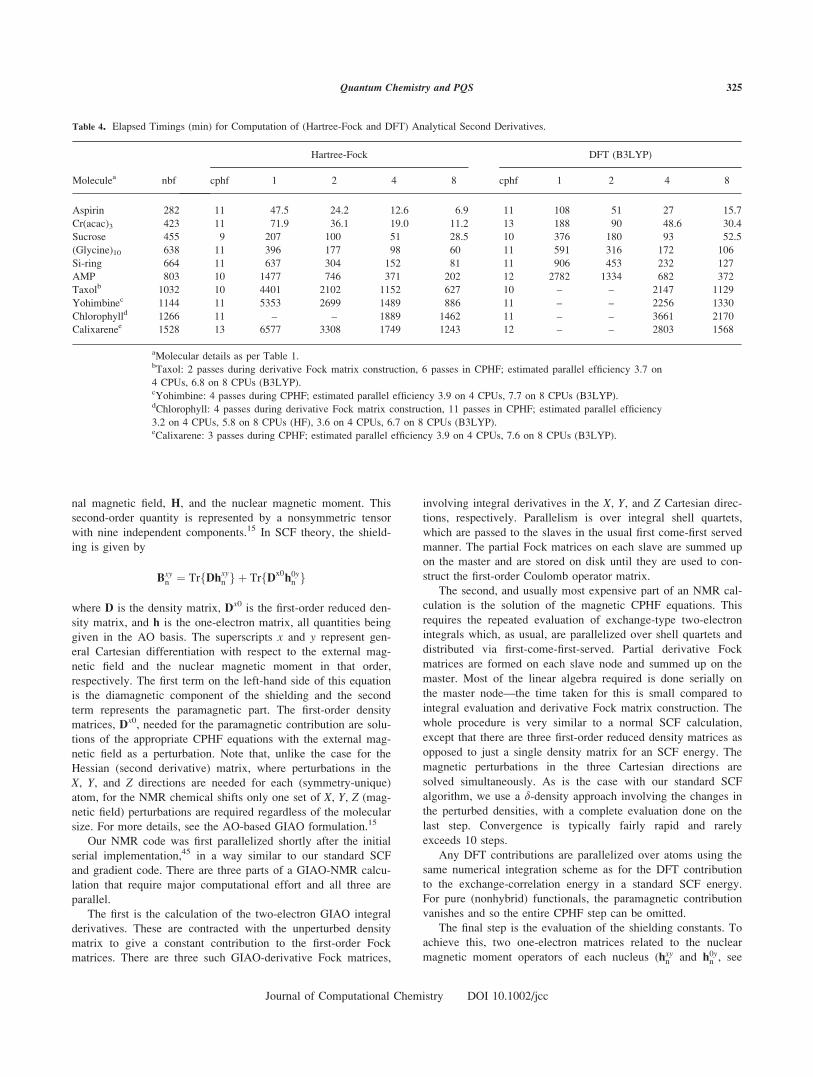
Analytical Second Derivatives

Our implementation of parallel Hartree-Fock and DFT analytical

second derivatives has been described in some detail in ref. 42.

We have also commented upon the importance of including the

quadrature weight derivatives in DFT Hessians for the computa-

tion of reliable vibrational frequencies.43

The parallel second derivative algorithm follows to a large

extent the structure of the parallel energy and gradient code.

All integrals and their derivatives, where required (both first

and second derivatives), are parallelized over shell quartets.

DFT quantities are coarsely parallelized over atoms. In both

cases, computed quantities are incorporated into local copies

of relevant matrices/arrays, followed by global summation of

all partial quantities on the master node. Derivative Fock mat-

rices, computed using integral first derivatives, are saved on

disk.

The additional complicating feature for analytical Hessians is

solution of the coupled perturbed Hartree-Fock (CPHF) equa-

tions. These are solved iteratively and require calculation of all

the non-negligible two-electron integrals (or at least the Cou-

lomb integrals) at each iteration (similar to a SCF energy) plus

additional terms for DFT wavefunctions. The CPHF equations

must be solved for each perturbation, i.e., for x, y, and z dis-

placements for each symmetry-unique atom, of which there are

potentially 3N, where N is the number of atoms (if there is no

usable symmetry). Solution of the CPHF equations also requires

reading back the derivative Fock matrices for each perturbation

on potentially each iteration. Note that all quantities are stored,

and the CPHF equations solved, directly in the atomic orbital

(AO) basis44; no integral transformations are required.

Solving the CPHF equations is the most computationally

demanding step in Hessian evaluation for larger molecules,

requiring considerable data transfer between nodes (there being

potentially 3N first-order density matrices, one for each perturba-

tion, as opposed to just one zeroth-order density matrix for an

SCF energy) as well as a significant amount of memory and

disk I/O. All the communication obviously contributes to a

reduction in parallel efficiency. Additionally, most of the matrix

algebra involved in actually solving the CPHF equations is se-

rial, although we have parallelized some of the more demanding

matrix operations.42

There are two computational steps with large memory

requirements (proportional to Nn2 where N 5 number of nu-

clear coordinates and n 5 number of basis functions). Both

involve the formation of partial derivative Fock matrices. The

first is from the zeroth-order density matrix and the first-deriv-

ative integrals. This has to be done only once. The second is

from the first-order perturbed densities and zeroth-order inte-

grals. The memory demand for this second step is asymptoti-

cally twice as big as for the first one and it has to be repeated

in every CPHF iteration. If the available memory is insuffi-

cient to hold all matrices in core simultaneously, then multiple

passes are made, e.g., solving for as many atoms in the CPHF

step as can be handled comfortably in one pass. This requires

the multiple evaluation of integrals or integral derivatives, but

it seldom introduces a significant penalty if the available mem-

ory is sufficient to handle a decent number of perturbations

per pass. Alternative memory models that store only part of

the derivative Fock matrices on the slaves may offer signifi-

cant advantages in this step.

We have implemented, and can utilize, Abelian point

group symmetry during integral and integral derivative calcula-

tion, and full point group symmetry during solution of the

CPHF equations, i.e., we solve for symmetry unique atoms only.

Despite the inefficiencies mentioned, the overall parallel effi-

ciency of our Hessian code is reasonably good, as can be seen

from the timings given in Table 4. For the larger systems, given

the long run times required for serial execution, we ran 4- and

8-processor jobs only, and provide an estimated parallel

efficiency.35

NMR Chemical Shifts

The magnetic shielding constant for nucleus n, Bn, is the second

derivative of the molecular energy with respect to both an exter-

Table 3. Elapsed Timings (min) for Computation of Hartree-Fock and DFT Analytical Gradients.

Moleculea nbf


1 2 4 8 16 1 2 4 8 16

Aspirin 282 2.0 1.0 0.52 0.27 0.15 3.0 1.6 0.80 0.43 0.26

Cr(acac)3 423 2.8 1.4 0.77 0.42 0.24 5.7 2.9 1.55 0.82 0.55

Sucrose 455 5.2 2.6 1.37 0.72 0.39 8.2 4.4 2.21 1.14 0.62

(Glycine)10 638 7.5 3.8 2.0 1.1 0.6 9.4 4.8 2.6 1.3 0.7

Si-ring 664 27.5 14.0 7.3 3.8 2.0 33.8 18.1 8.9 4.7 2.6

AMP 803 48.9 25.0 12.9 6.7 3.5 60.4 31.1 16.2 8.4 4.4

Taxol 1032 45.0 22.6 11.8 6.1 3.3 65.6 33.1 17.8 8.9 4.7

Yohimbine 1144 116 58.2 30.2 15.5 8.0 135 74.6 37.1 18.9 9.8

Chlorophyll 1266 50.7 26.0 12.7 6.7 3.6 72.4 34.7 18.2 9.5 5.1

Calixarene 1528 87.4 45.9 22.7 11.9 6.4 105 52.5 26.2 13.9 8.1

aMolecular details as per Table 1.



nal magnetic field, H, and the nuclear magnetic moment. This

second-order quantity is represented by a nonsymmetric tensor

with nine independent components.15 In SCF theory, the shield-

ing is given by

Bxyn ¼ TrfDhxyn g þ TrfDx0

h0yn g

where D is the density matrix, Dx0 is the first-order reduced den-

sity matrix, and h is the one-electron matrix, all quantities being

given in the AO basis. The superscripts x and y represent gen-

eral Cartesian differentiation with respect to the external mag-

netic field and the nuclear magnetic moment in that order,

respectively. The first term on the left-hand side of this equation

is the diamagnetic component of the shielding and the second

term represents the paramagnetic part. The first-order density

matrices, Dx0, needed for the paramagnetic contribution are solu-

tions of the appropriate CPHF equations with the external mag-

netic field as a perturbation. Note that, unlike the case for the

Hessian (second derivative) matrix, where perturbations in the

X, Y, and Z directions are needed for each (symmetry-unique)

atom, for the NMR chemical shifts only one set of X, Y, Z (mag-

netic field) perturbations are required regardless of the molecular

size. For more details, see the AO-based GIAO formulation.15

Our NMR code was first parallelized shortly after the initial

serial implementation,45 in a way similar to our standard SCF

and gradient code. There are three parts of a GIAO-NMR calcu-

lation that require major computational effort and all three are

parallel.

The first is the calculation of the two-electron GIAO integral

derivatives. These are contracted with the unperturbed density

matrix to give a constant contribution to the first-order Fock

matrices. There are three such GIAO-derivative Fock matrices,

involving integral derivatives in the X, Y, and Z Cartesian direc-

tions, respectively. Parallelism is over integral shell quartets,

which are passed to the slaves in the usual first come-first served

manner. The partial Fock matrices on each slave are summed up

on the master and are stored on disk until they are used to con-

struct the first-order Coulomb operator matrix.

The second, and usually most expensive part of an NMR cal-

culation is the solution of the magnetic CPHF equations. This

requires the repeated evaluation of exchange-type two-electron

integrals which, as usual, are parallelized over shell quartets and

distributed via first-come-first-served. Partial derivative Fock

matrices are formed on each slave node and summed up on the

master. Most of the linear algebra required is done serially on

the master node—the time taken for this is small compared to

integral evaluation and derivative Fock matrix construction. The

whole procedure is very similar to a normal SCF calculation,

except that there are three first-order reduced density matrices as

opposed to just a single density matrix for an SCF energy. The

magnetic perturbations in the three Cartesian directions are

solved simultaneously. As is the case with our standard SCF

algorithm, we use a d-density approach involving the changes in

the perturbed densities, with a complete evaluation done on the

last step. Convergence is typically fairly rapid and rarely

exceeds 10 steps.

Any DFT contributions are parallelized over atoms using the

same numerical integration scheme as for the DFT contribution

to the exchange-correlation energy in a standard SCF energy.

For pure (nonhybrid) functionals, the paramagnetic contribution

vanishes and so the entire CPHF step can be omitted.

The final step is the evaluation of the shielding constants. To

achieve this, two one-electron matrices related to the nuclear

magnetic moment operators of each nucleus (hxyn and h0yn , see

Table 4. Elapsed Timings (min) for Computation of (Hartree-Fock and DFT) Analytical Second Derivatives.

Moleculea nbf


cphf 1 2 4 8 cphf 1 2 4 8

Aspirin 282 11 47.5 24.2 12.6 6.9 11 108 51 27 15.7

Cr(acac)3 423 11 71.9 36.1 19.0 11.2 13 188 90 48.6 30.4

Sucrose 455 9 207 100 51 28.5 10 376 180 93 52.5

(Glycine)10 638 11 396 177 98 60 11 591 316 172 106

Si-ring 664 11 637 304 152 81 11 906 453 232 127

AMP 803 10 1477 746 371 202 12 2782 1334 682 372

Taxolb 1032 10 4401 2102 1152 627 10 – – 2147 1129

Yohimbinec 1144 11 5353 2699 1489 886 11 – – 2256 1330

Chlorophylld 1266 11 – – 1889 1462 11 – – 3661 2170

Calixarenee 1528 13 6577 3308 1749 1243 12 – – 2803 1568

aMolecular details as per Table 1.bTaxol: 2 passes during derivative Fock matrix construction, 6 passes in CPHF; estimated parallel efficiency 3.7 on

4 CPUs, 6.8 on 8 CPUs (B3LYP).cYohimbine: 4 passes during CPHF; estimated parallel efficiency 3.9 on 4 CPUs, 7.7 on 8 CPUs (B3LYP).dChlorophyll: 4 passes during derivative Fock matrix construction, 11 passes in CPHF; estimated parallel efficiency

3.2 on 4 CPUs, 5.8 on 8 CPUs (HF), 3.6 on 4 CPUs, 6.7 on 8 CPUs (B3LYP).eCalixarene: 3 passes during CPHF; estimated parallel efficiency 3.9 on 4 CPUs, 7.6 on 8 CPUs (B3LYP).



the shielding equation above) need to be formed, contracted

with the unperturbed and the first-order reduced density matri-

ces, respectively, and the trace of the resulting matrices taken.

This has a non-negligible computational cost and is parallelized

over the nuclei.

Timings for NMR shielding calculations on our test set are

shown in Table 5 (the open-shell system Cr(acac)3 has been

omitted as our NMR code is closed-shell only). Parallel efficien-

cies are high and are similar to those for the SCF energy

(Table 1). The absolute timings are also very close for both HF

and DFT wavefunctions; the extra time required to compute the

DFT contributions are balanced by the reduction in the number

of cycles required to solve the CPHF equations (see Table 5).

For pure DFT functionals the timings would of course be much

less, as no CPHF step would be required. Comparing the time

required for the corresponding SCF energy (Table 1) with the

NMR times (Table 4), shows that the latter typically take only

slightly longer than the former, attesting to the overall efficiency

(both serial and parallel) of our NMR code.

Second-Order Møller-Plesset Perturbation Theory (MP2)

Our implementation of second-order Møller-Plesset perturbation

theory (MP2) energies was first presented in 2001.46 It is based

on the Saebo-Almlof direct-integral transformation,47 coupled

with an efficient prescreening of the AO integrals. We recently

presented an efficient implementation of the MP2 gradient based

on the same approach.48 At the time of writing, our MP2 gradi-

ent code is (still) not parallel, so we concentrate on the energy,

which was parallelized in 2002.49

The closed-shell MP2 energy can be written as50

EMP2 ¼X

i�j

eij ¼X

i�j

ð2�dijÞX

a;b

ðaijbjÞ½2ðaijbjÞ � ðbijajÞ�

=ðei þ ej � ea � ebÞwhere i and j denote doubly-occupied molecular orbitals (MOs),

a and b denote virtual (unoccupied) MOs, and e are the corre-

sponding orbital energies. This form of the MP2 energy requires

an integral transformation from the original AO- to the MO-ba-

sis, and in the Saebo-Almlof method this is accomplished via

two half-transformations, involving first the two occupied MOs

and then the two virtuals. The AO-integral (lm|kr) is consideredas the (mr) element of a generalized exchange matrix X

lk, and

the two half-transformations can be formulated as matrix multi-

plications:

ðlijkjÞ ¼ Ylkij ¼

X

v;r

CTviX

lkvrCrj ¼ CT

i XlkCj

ðaijbjÞ ¼ Zijab ¼

X

l;k

CTlaY

ijlkCkb ¼ CT

aYijCb

The disadvantage of this approach—that the full permuta-

tional symmetry of the AO-integrals cannot be utilized—is

more than offset by the increased efficiency of the matrix for-

mulation, especially for larger systems. The dominant compu-

tational step is the first matrix multiplication that scales for-

mally as nN4; subsequent transformations scale as n2N3 where

n 5 the number of correlated occupied molecular orbitals, and

N 5 the number of atomic orbitals; usually N�n. An impor-

tant contribution to the efficiency of our code is the utilization

of the sparsity of the AO integral matrices X. This can be

done without resorting to sparse matrix techniques that are

usually many times slower (though better scaling) than dense

matrix multiplication routines. The sparsity pattern of the mat-

rices X is such that entire rows and columns are zero; these

can be removed and the AO matrices X compressed to give

smaller dense matrices46 that can use highly efficient dense

matrix multiplication routines. This feature makes our MP2

program often competitive with approximate techniques, such

as density fitting (‘‘RI’’) MP2.

As each half-transformed integral matrix Ylk is formed,

its nonzero elements are written to disk (in compressed

format, as 5-byte integers49). In the second half-transforma-

tion, the Ylkij (which contain all indices i,j for a given l,k pair)

have to be reordered into Yijlk (all indices l,k for a given i,j

pair); this is accomplished via a modified Yoshimine bin

sort.51

Table 5. Elapsed Timings (min) for Computation of (Hartree-Fock and DFT) NMR Chemical Shifts.

Moleculea nbf


cphf 1 2 4 8 16 cphf 1 2 4 8 16

Aspirin 282 7 8.9 4.2 2.1 1.1 0.6 5 7.4 3.5 1.8 1.0 0.6

Sucrose 455 7 22.2 10.6 5.3 2.8 1.5 5 19.7 9.4 4.8 2.7 1.4

(Glycine)10 638 8 25.9 12.4 6.3 3.5 2.0 6 23.1 11.7 6.0 3.5 2.0

Si-ring 664 8 112 52 25.5 13.3 6.9 6 99 49 25 13.2 9.0

AMP 803 9 207 100 49 25.3 13.1 6 180 85 43 23.0 14.7

Taxol 1032 8 240 116 53 28.0 15.1 6 209 105 53 26 13.7

Yohimbine 1144 9 510 256 128 65 33 6 486 242 122 58 30.0

Chlorophyll 1266 9 197 102 54 28.7 15.8 7 227 114 58 28 15.5

Calixarene 1528 9 449 194 97 51 27.0 6 403 204 103 45 24.3




The overall scheme is straightforward to implement provided

there is enough memory to store a (potentially) complete Xlk

exchange matrix and enough disk storage to hold all possible

(compressed) Ylk matrices, i.e., all the first half-transformed

integrals. Note that, unlike many other MP2 algorithms (e.g.,

ref. 52), the fast memory requirement in the Saebo-Almlof

scheme scales only quadratically with basis size. However, for

reasons of efficiency, the AO integrals are calculated in batches

over complete shells, and this requires s2N2 double words of fast

memory (where N is the number of basis functions and s is the

shell size, i.e., s 5 1 for s-shells, s 5 3 for p-shells, s 5 5 for

(spherical) d-shells, etc). Symmetry can easily be utilized in the

first half-transformation (not so easily in the second) by calculat-

ing only those integrals (lm|kr), which have symmetry-unique

shell pairs M,L where l [ M, k [ L.In the parallel algorithm, the first-half transformation is read-

ily parallelized by looping over (symmetry unique) M,L shell

pairs, sending each shell pair to a different slave in the usual

first come-first served fashion. The half-transformed integrals

(the matrices Ylk) are written directly to local disk storage on

the node on which they were computed. This part of the paral-

lel algorithm is very efficient as the only data that is transmit-

ted over the network are the shell indices. At the end of the

first half-transformation, all the Ylk matrices are distributed

approximately equally on local storage over all the slave

nodes.

In the original parallel algorithm,49 the bin sort required

prior to the second half-transformation was accomplished by

spawning a second (‘‘bin write’’ or ‘‘bin listen’’) process on ev-

ery slave node. Each slave then commenced a standard Yoshi-

mine bin sort of the Ylk matrices stored on its own disk; how-

ever, whenever a particular bin for a given i,j pair was full,

instead of writing it to disk on the same slave, it was sent to

the ‘‘bin write’’ process running on the slave that the i,j pair

had been assigned to. The total number of i,j pairs is, of

course, known in advance, and is divided into the number of

slaves, so each slave is assigned a certain subset of the total.

The ‘‘bin write’’ process on the appropriate slave then writes

the bin to its own local disk. At the end of the sort, all the

‘‘bin write’’ processes are killed, and each slave will have a

roughly equal number of Yij matrices, distributed in various

bins in a direct access file, containing all l,k pairs for the sub-

set of i,j pairs that are on its disk. The complete Yij matrices

are then constructed from the individual bins and the second

half-transformation carried out. Each slave then computes a

partial pair-correlation energy sum, eij, and the partial sums are

sent back to the master for the final summation to give the full

MP2 correlation energy.

In the current algorithm, we have eliminated the spawned

‘‘bin write’’ processes. Instead we have modified the sorting step

to include polling (this is a well-established procedure within

the message-passing paradigm53). When a bin is full it is sent to

the appropriate slave directly, without going via the spawned

‘‘bin write’’ process. While they are performing the bin sort, the

slave nodes periodically poll the network for incoming bins.

Any such bins that are detected have priority, and are received

and written to disk. When the write is complete, the slave con-

tinues with its own local bin sort.

This change does not make the sorting algorithm any more

complex. Despite the fact that a part of the write scheduling is

done internally in the sorting algorithm itself, whereas in the

case of the spawned ‘‘bin write’’ it was done by the operating

system, there is no significant performance hit, as the limiting

factor is usually disk access in both cases. In fact, a slight

improvement can often be observed on a small number of nodes,

since bins destined for the same node are written to local disk

directly instead of being relayed via the ‘‘bin write’’ process.

This procedure is quite similar to the original algorithm and

avoids spawning the additional processes. As mentioned in the

Introduction section, we had considerable difficulty with the

spawning in the MPI version (PVM was fine) and this difficulty

was the main incentive for the change, which has had negligible

effect on program efficiency.

We have made two other improvements to the parallel algo-

rithm as originally presented.49 In the original serial algorithm,46

the integral compression scheme involved dividing the integral

value by the integral neglect threshold and storing the result as a

4-byte integer. This effectively reduces the disk space required

for integral storage by half compared to storing a full 8-byte

real. However, the value of the integral threshold is somewhat

limited in this simple scheme, as if the threshold is too small

there is a risk of integer overflow if the integral value is large

(the largest integer that can be stored in a 4-byte word is 231,

allowing one byte for the sign; this is about a billion, 109). We

already modified this scheme for the parallel algorithm by allow-

ing an extra byte for integral storage, effectively mimicking a 5-

byte integer, where the additional byte stores the number of

times 231 exactly divides the integral (in integer form), with the

remainder being stored in 4 bytes. This slightly increases the in-

tegral packing/unpacking time, and increases disk storage by

25% during the first half-transformation, but allows a tightening

of the integral threshold by over two-and-a-half orders of

magnitude.

We have now modified this even further by effectively allow-

ing for a variable integral neglect threshold for those integrals

which are still too large even for the 5-byte integer storage. If

the current threshold causes an overflow, then it is reduced (or

increased, depending on your point of view) by a power of 10

(from 102x to 102(x–1)) until the integral can be safely stored

without overflow. This is done only for those (few) integrals

that cause problems with the existing neglect threshold, which is

used unchanged for all the other integrals. Of course, during in-

tegral unpacking, the modified threshold is used when unpacking

that integral. This scheme has minimal effect on numerical accu-

racy, as normally only a very small percentage of integrals are

so treated, and ensures that all integrals can be stored without

overflow.

The other change is in the mechanics of the second half-

transformation. This was formerly done for a single i,j pair at atime, by reading all the i,j bins from the direct-access file, form-

ing the full Yij matrix, and doing the second half-transformation

on that matrix. If there are a large number of i,j pairs, then the

bin (record) size is correspondingly small, and a relatively large

number of records need to be located and read from the direct-

access file in order to form each Yij matrix. This results in a

small CPU/IO ratio and an inefficient transformation. The solu-



tion is to reduce the number of reads by increasing the record

size (writing the same data in large chunks is more efficient

than writing it in small chunks, as it can be located and retrieved

with many fewer reads). This is done by grouping several i,jpairs together and writing them in a single record. As soon as a

given bin corresponding to one i,j pair is full, then all bins for

all the i,j pairs in that group are written, whether they are full or

not. There is a small penalty associated with the writing of

incompletely full bins, but this is more than offset by the group-

ing together of i,j pairs and the consequent formation and trans-

formation of several Yij matrices simultaneously.

Table 6 shows timings for single-point MP2 energies starting

from the converged SCF wavefunction, i.e., timings are for the

MP2 part only and do not include the SCF time. Also shown in

Table 6 are ncor—the number of correlated orbitals and nvir—

the number of virtual orbitals. By default the core orbitals,

which we take as all SCF orbitals with orbital energies below

23.0 Eh, are excluded from the calculation.

As can be seen from Table 6, parallel efficiencies for MP2

energies are very good, being over 14 on 16 CPUs for all the

larger systems (Si-ring and above). The smaller systems (aspirin,

sucrose) have poor parallel efficiencies, mainly due to overhead

in the parallel bin sort during the second half-integral

transformation.

There is one more feature of the parallel MP2 algorithm that

should be noted. For the algorithm to work, all half-transformed

integrals must be computed and written to disk. Parallel runs

have available the aggregate disk storage over all the nodes

being utilized and hence can store more integrals, and handle

larger systems, than serial jobs. The default disk storage for the

various scratch files (mainly for the first half-transformed inte-

grals) is 50 GB; this was increased to 250 GB for the serial runs

for both chlorophyll and calixarene as the default was insuffi-

cient. The additional disk storage available improved the per-

formance of the bin-sort in the second half-integral transforma-

tion, making the serial jobs faster relative to the parallel jobs

(where only 50 GB was available in total per node) than they

otherwise would have been.

For large basis set calculations, in particular for large MP2

calculations, dual-basis methods can decrease the computational

cost without affecting the results significantly. Such methods

have been implemented for multireference54 and single refer-

ence55 MP2, and recently also for resolution-of-identity (RI)

MP2.56 The dual basis method can also significantly reduce the

cost of the underlying Hartree-Fock calculation55; this is impor-

tant as the computational cost of MP2 in modern programs is of-

ten less than that of the corresponding SCF. The dual-basis Har-

tree-Fock method can be readily generalized to DFT.57,58

PQS currently has dual-basis Hartree-Fock, DFT and MP2

implemented.

The Fourier Transform Coulomb Method

The FTC method is a relatively recent procedure for fast and

accurate DFT calculations, particularly with large basis sets. The

algorithm for the energy was presented in 200259 and for the

gradient a year later.60 The energy was first parallelized in

2004,61 and the parallel gradient was presented very recently.62

The FTC method derives from earlier work by Parrinello and

coworkers under the acronym GAPW (Gaussian and Augmented

Plane Waves), initially for pseudopotential methods,63 and sub-

sequently for all-electron calculations.64 It shares the goals and

the basic idea behind the GAPW approach, but is quite different

technically. It can be considered as being related to the so-called

resolution of the identity RI-DFT approach, which expands the

density in an auxiliary basis.65 However, unlike the situation in

RI-DFT where the auxiliary basis is typically a set of Gaussian

functions slightly larger than the original basis set,66 in the FTC

method it is an essentially infinite plane wave basis. This makes

FTC potentially much more accurate than standard RI-DFT. It

also scales better with respect to both system and basis size.

The method derives its efficiency from the fact that the Cou-

lomb operator is diagonal in momentum space and almost effort-

less switching between momentum space and direct (coordinate)

space can be achieved via fast Fourier transform (FFT). The

dominant part of the traditional Coulomb term can be evaluated

in plane wave space very efficiently (up to two orders of magni-

tude and more faster than with our standard all-integral algo-

rithm), leaving only a small residual originating from compact,

core-like basis functions to be evaluated in the traditional or in

some other way. We have already demonstrated that a complete

geometry optimization of yohimbine with a fairly large basis set

(1275 basis functions) can be accomplished in parallel five times

Table 6. Elapsed Timings (min) for Computation of the (Restricted) MP2 Energy.

Moleculea nbf ncor nvir 1 2 4 8 16

Aspirin 282 34 235 5.1 2.6 1.5 1.2 1.1

Sucrose 455 68 364 25.4 12.7 6.8 4.0 3.0

(Glycine)10 638 114 524 72.8 35.8 18.0 9.3 5.3

Si-ring 664 53 570 179 86.0 42.4 22.0 12.0

AMP 803 63 713 254 125 61.1 31.8 16.4

Taxol 1032 164 806 623 311 164 83.5 43.3

Yohimbine 1144 69 1049 679 338 170 86.1 43.5

Chlorophyllb 1266 175 1025 989 505 258 140 69.9

Calixareneb 1528 92 1400 672 342 169 86.1 44.3

aMolecular details as per Table 1.bIncreased disk storage requested for serial jobs.



faster than with our classical all-integral algorithm62 (the

speedup in the Coulomb part is well over an order of magni-

tude). The efficiency of our current FTC code is limited by pro-

gram steps that are performed in the traditional way. These

steps can be improved to become commensurate in efficiency

with the FTC Coulomb program, and work along these lines is

being conducted both at PQS and elsewhere.67 For instance,

the Coulomb contribution of compact charge densities, which

is currently calculated by the traditional electron repulsion inte-

gral method, is ideally suited to calculation through a multipole

expansion, as the core-like densities are largely spherical and

are dominated by low-order multipoles. With this change and

improvements in the calculation of the exchange-correlation

contribution, further significant savings should easily be

achievable.

Details of the FTC method and its parallelization can be

found in refs. 61 and 62. One thing to note is that, as the

method involves an alternative procedure to evaluate the Cou-

lomb term, it cannot be used to any real advantage for hybrid

density functionals, such as B3LYP, which contain a percentage

of the ‘‘exact’’ Hartree-Fock exchange. Despite much research,

there is still no method for calculating the exact (Hartree-Fock)

exchange term with anywhere near the same efficiency as the

Coulomb term. In principle, the exact exchange becomes line-

arly scaling asymptotically in insulators.68,69 However, the cross-

over point is very high, especially in three-dimensional systems,

and in practice there are few alternatives to the traditional elec-

tron repulsion integral method, regardless of claims to the con-

trary.

Table 7 provides timings for single-point energy plus gradi-

ent calculations using the OLYP30 functional comparing our cur-

rent (sub-optimal) FTC code with the classical all-integral algo-

rithm. Note that Cr(acac)3 has been omitted as our FTC code is

currently closed-shell only and calixarene (C2h) has been omitted

as we have not yet implemented symmetry.

Timings are reported in Table 7 for the SCF energy (top

number in each row) and the gradient (bottom number) sepa-

rately. In all cases except for (glycine)10 both energy and gradi-

ent calculation are faster with the FTC algorithm, ranging from

only slightly faster (aspirin) to about 3.5 times faster (yohim-

bine). The nature of the FTC method is such that the greatest

savings are achieved with the largest basis sets; due to current

algorithm inefficiencies there are little or no savings with small

to modest basis sets. The smallest basis set we have utilized is

6-31G*, which was used for (glycine)10, so it is not surprising

that this molecule—which is also a very extended system—

shows no savings over the classical algorithm.

The parallel efficiency of the FTC energy is not as great as

with the classical algorithm (although the FTC gradient almost

is62) and so the advantage of the FTC algorithm over the classi-

cal decreases as the degree of parallelism (number of CPUs

used) increases. This can be seen in particular for aspirin where

in serial and on two CPUs computing the FTC energy is slightly

faster than calculating the all-integral energy, but on four and

eight CPUs this has switched.

One of the major advantages of the FTC algorithm over

other related approximate methods is its high accuracy. Table 7

also shows the difference in the final converged SCF energy

between the classical algorithm (EDFT) and the FTC algorithm

(EFTC). For five of the eight molecules, including the three

largest, this difference is 1 lEh or less. The greatest error (still

less than 0.2 mEh) is with Si3AlO12H8Cu (Si-ring); this is not

surprising as this molecule has five post-first row atoms includ-

ing copper. We know of no other method that can provide

computational savings while at the same time maintaining such

high accuracy.

Table 7. Elapsed Timings (min) for Computation of Single-Point OLYP FTC Energies and Gradients.

Moleculea nbf EDFT 2 EFTC

Classical algorithmb FTC algorithmb

1 2 4 8 1 2 4 8

Aspirin 282 0.000000 7.7 3.9 1.9 1.1 6.2 3.6 2.1 1.4

3.2 1.6 0.8 0.4 2.3 1.3 0.7 0.4

Sucrose 455 0.000000 18.9 9.5 4.9 2.5 14.7 8.1 4.4 2.5

8.7 4.4 2.3 1.2 7.8 4.2 2.2 1.1

(Glycine)10 638 20.000035 19.8 10.7 5.4 3.1 23.8 12.8 7.1 4.6

10.4 5.1 2.5 1.4 10.4 5.1 2.6 1.4

Si-ring 664 20.000196 121 60.5 30.8 15.8 40.1 20.7 11.3 6.6

36.4 17.8 9.3 4.7 13.4 6.9 3.6 2.0

AMP 803 0.000124 198 99.1 49.0 25.6 60.6 31.3 16.7 9.4

63.6 32.0 16.0 8.3 22.6 11.6 6.1 3.2

Taxol 1032 0.000001 165 83.1 41.5 22.1 111 60.2 30.8 17.2

71.2 35.4 17.5 9.1 54.0 29.3 14.4 7.6

Yohimbine 1144 0.000001 504 253 127 64.6 146 79.0 41.6 22.5

146 72.7 38.5 18.8 51.1 26.8 13.9 7.2

Chlorophyll 1266 20.000001 226 121 60.7 32.8 145 75.0 39.5 22.9

68.1 36.0 18.0 9.4 51.6 26.1 13.1 7.0

aMolecular details as per Table 1.bTimings in each row are for energies (top) and gradients (bottom).



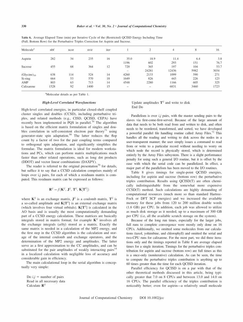
High-Level Correlated Wavefunctions

High-level correlated energies, in particular closed-shell coupled

cluster singles and doubles (CCSD), including perturbative tri-

ples, and related methods (e.g., CISD, QCISD, CEPA) have

recently been implemented in PQS in parallel.70 The algorithm

is based on the efficient matrix formulation of singles and dou-

bles correlation in self-consistent electron pair theory71 using

generator-state spin adaptation.50 The latter reduces the flop

count by a factor of two for the pair coupling terms compared

to orthogonal spin adaptation, and significantly simplifies the

formulae. The matrix formulation is ideal for modern worksta-

tions and PCs, which can perform matrix multiplications much

faster than other related operations, such as long dot products

(DDOT) and vector linear combinations (DAXPY).

The reader is referred to the original presentation70 for details,

but suffice it to say that a CCSD calculation comprises mainly of

loops over i,j pairs, for each of which a residuum matrix is com-

puted. This residuum matrix can be expressed as follows:

Rij ¼ f ðKij; Jij; Tij; K½Tij�Þ

where Kij is an exchange matrix, Jij is a coulomb matrix, Tij is

a so-called amplitude and K[Tij] is an external exchange matrix

(which involves four virtual orbitals). K[Tij] is calculated in the

AO basis and is usually the most computationally demanding

part of a CCSD energy calculation. These matrices are basically

integrals stored in matrix format; for example Kij involves all

the exchange integrals (ai|bj) stored as a matrix. Exactly the

same matrix is needed in a calculation of the MP2 energy, and

the first step in the CCSD algorithm is the calculation and stor-

age of the internal coulomb and exchange operators, and the

determination of the MP2 energy and amplitudes. The latter

serve as a first approximation to the CC amplitudes, and can be

substituted for the pair amplitudes of weakly interacting pairs14

in a localized calculation with negligible loss of accuracy and

considerable gain in efficiency.

The main calculational loop in the serial algorithm is concep-

tually very simple:

Do i,j 5 number of pairs

Read in all necessary data

Calculate Rij

Update amplitudes Tij and write to disk

End Do

Parallelism is over i,j pairs, with the master sending pairs to the

slaves via first-come-first-served. Because of the large amount of

data that needs to be both read from and written to disk, and often

needs to be reordered, transformed, and sorted, we have developed

a powerful parallel file handling routine called Array Files.72 This

handles all the reading and writing to disk across the nodes in a

user-transparent manner; the user simply issues a command to read

from or write to a particular record without needing to worry on

which node the record is physically stored, which is determined

entirely by the Array Files subsystem. There is a slight performance

penalty for using such a general I/O routine, but it is offset by the

ease with which the serial code can be parallelized. In effect, a

major part of the parallelism has been moved to the I/O routines.

Table 8 gives timings for single-point QCISD energies,

including for aspirin and sucrose (bottom row) the perturbative

triples contribution. Results using QCISD(T) are often chemi-

cally indistinguishable from the somewhat more expensive

CCSD(T) method. Such calculations are highly demanding of

computational resources (much more so than standard Hartree-

Fock or DFT SCF energies) and we increased the available

memory for these jobs from 120 to 200 million double words

(1.6 GB) per CPU. In addition, each job was allowed to utilize

as much disk storage as it needed, up to a maximum of 300 GB

per CPU (i.e, all the available scratch storage on the system).

Because of the long run times, especially for the larger jobs,

full runs to complete convergence were mostly only done on 16

CPUs. Additionally, we omitted some molecules from our calcula-

tions (taxol, yohimbine, and chlorophyll) and omitted the serial and

two-CPU runs for calixarene. For the most part, we did three itera-

tions only and the timings reported in Table 8 are average elapsed

times for a single iteration. Timings for the perturbative triples con-

tribution for aspirin and sucrose (bottom row) are full times as this

is a once-only (noniterative) calculation. As can be seen, the time

to compute the perturbative triples contribution is anything up to

60 times greater than the time for each QCISD iteration.

Parallel efficiency for QCISD is on a par with that of the

other theoretical methods discussed in this article, being typi-

cally greater that 7.0 on 8 CPUs and between 13.0 and 14.0 on

16 CPUs. The parallel efficiency of the triples contribution is

noticeably better; even for aspirin—a relatively small molecule

Table 8. Average Elapsed Time (min) per Iterative Cycle of the (Restricted) QCISD Energy Including Time

(Full; Bottom Row) for the Perturbative Triples Correction for Aspirin and Sucrose.

Moleculea nbf ncor nvir iter 1 2 4 8 16

Aspirin 282 34 235 16 35.0 18.9 11.4 6.4 3.8

1196 602 293 151 76.7

Sucrose 455 68 364 12 720 365 197 104 53.7

– 24281 12436 5982 3034

(Glycine)10 638 114 524 14 4260 2133 1099 590 271

Si-ring 664 53 570 18 1649 826 443 226 123

AMP 803 63 713 14 4548 2280 1166 605 325

Calixarene 1528 92 1400 15 – – 6831 3460 1723




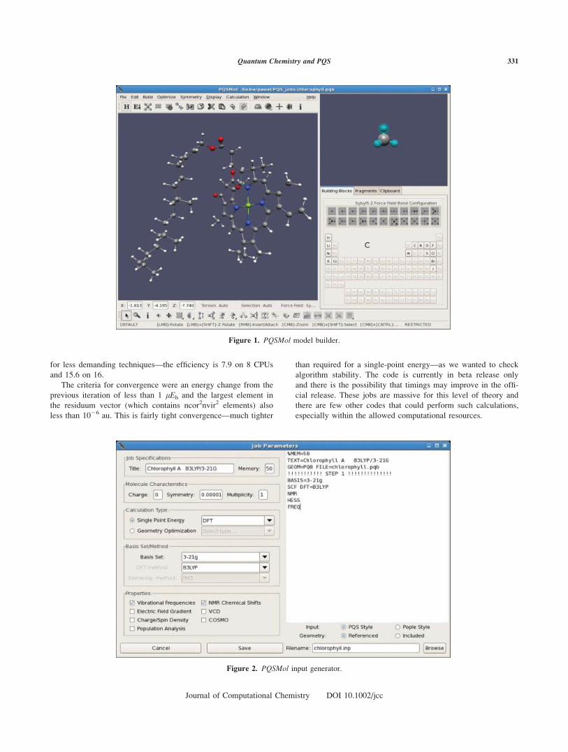
for less demanding techniques—the efficiency is 7.9 on 8 CPUs

and 15.6 on 16.

The criteria for convergence were an energy change from the

previous iteration of less than 1 lEh and the largest element in

the residuum vector (which contains ncor2nvir2 elements) also

less than 1026 au. This is fairly tight convergence—much tighter

than required for a single-point energy—as we wanted to check

algorithm stability. The code is currently in beta release only

and there is the possibility that timings may improve in the offi-

cial release. These jobs are massive for this level of theory and

there are few other codes that could perform such calculations,

especially within the allowed computational resources.

Figure 1. PQSMol model builder.

Figure 2. PQSMol input generator.



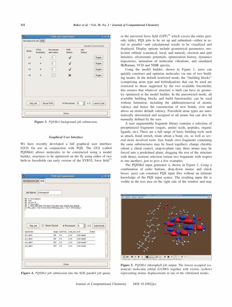
Graphical User Interface

We have recently developed a full graphical user interface

(GUI) for use in conjunction with PQS. The GUI (called

PQSMol) allows molecules to be constructed using a model

builder, structures to be optimized on the fly using either of two

built-in forcefields (an early version of the SYBYL force field73

or the universal force field (UFF)74 which covers the entire peri-

odic table), PQS jobs to be set up and submitted—either in se-

rial or parallel—and calculational results to be visualized and

displayed. Display options include geometrical parameters, mo-

lecular orbitals (canonical, local, and natural), electron and spin

densities, electrostatic potentials, optimization history, dynamics

trajectories, animation of molecular vibrations, and simulated

IR/Raman, VCD and NMR spectra.

Using the model builder, shown in Figure 1, users can

quickly construct and optimize molecules via one of two build-

ing modes. In the default restricted mode, the ‘‘building blocks’’

(comprising atom type and hybridization) that can be used are

restricted to those supported by the two available forcefields;

this ensures that whatever structure is built can have its geome-

try optimized in the model builder. In the unrestricted mode, all

available building blocks and build functionality can be used

without limitation, including the addition/removal of atomic

valency and hence the construction of new bonds, over and

above an atoms default valency. Forcefield atom types are auto-

matically determined and assigned to all atoms but can also be

manually defined by the user.

A user augmentable fragment library contains a selection of

preoptimized fragments (sugars, amino acids, peptides, organic

ligands, etc). There are a full range of basic building tools such

as attach, bond stretch, rotate about a bond, etc, as well as sev-

eral more involved tools: fuse bonds (two fragments containing

the same substructures may be fused together), change chirality

(about a chiral center), snap-to-plane (any three atoms may be

forced into a predefined plane, dragging the rest of the structure

with them), reorient selection (orient two fragments with respect

to one another), just to give a few examples.

The PQSMol input generator is shown in Figure 2. Using a

combination of radio buttons, drop-down menus and check

boxes, users can construct PQS input files without an intimate

knowledge of the PQS input syntax. The resulting input file is

visible in the text area on the right side of the window and may

Figure 3. PQSMol background job submission.

Figure 4. PQSMol job submission into the SGE parallel job queue.

Figure 5. PQSMol chlorophyll job output. The lowest occupied (ca-

nonical) molecular orbital (LUMO) together with vectors (yellow)

representing atomic displacements in one of the vibrational modes.



be manually edited by more advanced users to include features

not yet supported in the GUI.

Jobs may be submitted in serial or parallel as background

processes or via a queuing system such as SGE (Sun grid

engine), DQS (distributed queuing system) or PBS (portable

batch system). All three are supported. Background job submis-

sion allows users full control of the PVM (parallel virtual

machine) on the cluster, including starting and stopping the

PVM daemon on each of the cluster nodes. Figure 3 shows back-

ground submission of a chlorophyll job requesting eight CPUs

on nodes n1, n2, and n3 of a four-node cluster, each of which

has four CPUs available. Node n4 is not used for this calculation.

Figure 4 shows the same job submitted into the SGE job queue

also requesting eight CPUs. The queuing system determines which

nodes in the cluster are used for the calculation.

Post-job visualization of the chlorophyll job output is

depicted in Figure 5. Shown is the lowest occupied (canonical)

molecular orbital (LUMO) together with vectors (yellow) repre-

senting atomic displacements in one of the vibrational modes.

An orbital energy plot and simulated IR and NMR spectra are

displayed in Figures 6–8, respectively. Orbital display options

allow users to change the isosurface level (without the need to

recalculate grid points) and to display cross sections of the sur-

face. Localized and natural orbitals as well as spin density can

be displayed, if calculated. The electrostatic potential may be

mapped on the electron density surface.

The vibrational spectrum display can show simulated IR,

Raman or VCD spectra, if calculated. The starting and ending

values (ppm) on simulated NMR spectra are user selectable, as

is the reference value for the chemical shifts. User adjustable

halfwidths are available on all simulated spectra to customize

the curve fitting and a zoom function allows particular portions

of the spectrum to be expanded. Additionally dynamics trajec-

tory and optimization history plots may be produced. Screen

shots of any graphical image may be saved to a.jpeg file for

easy incorporation into publications.

Conclusions

PQS is a fully parallel, primarily ab initio program package

offering efficient implementations of the most popular methods

Figure 6. PQSMol orbital energy plot for chlorophyll.

Figure 8. PQSMol simulated NMR spectrum for chlorophyll.

Shown is the 13C spectrum.

Figure 7. PQSMol simulated IR spectrum for chlorophyll.



of modern quantum chemistry. All PQS software, including the

new GUI (PQSMol) are available both as an integral part of our

parallel QuantumCubeTM computers1 or as separate stand-alone

packages. Both Linux and Windows versions are available. See

our website for details.

As demonstrated in this article, all of the major functionality

in PQS is fully parallel and has high parallel efficiency, with

factors of up to 7.9 on 8 CPUs and[15.0 on 16 CPUs. Calcula-

tions, which in many other programs would require prohibitive

amounts of computational resources (i.e., memory and/or disk

storage), can be completed with PQS with only modest resource

demands. New methodologies, such as the FTC method, offer

significant savings when compared with standard techniques

with essentially no loss in accuracy. Our software was designed

for use with small, inexpensive Linux-type clusters (such as our

QuantumCubeTM) which are currently very popular and which

are ideally suited for small research groups and individual

research workers, offering modest parallelism (8–32 CPUs) at

low cost.

References

1. PQS version 4.0, Parallel Quantum Solutions, 2013 Green Acres

Road, Suite A, Fayetteville, AR 72703. Email: [email protected];

URL: http://www.pqs-chem.com.

2. Meyer, W. Int J Quantum Chem Symp 1971, 5, 341.

3. Meyer, W. J. Chem Phys 1973, 58, 1017.

4. Pulay, P. Mol Phys 1969, 17, 197.

5. Meyer, W.; Pulay, P. Proceedings of the Second Seminar on Compu-

tational Quantum Chemistry, Strasbourg, France, 1972, p. 44.

6. Preuss, H. Z Naturforsch 1956, 11, 823.

7. Werner, H.-J.; Knowles, P. J. J Chem Phys 1985, 82, 5053.

8. Werner, H.-J., Reinsch, E. A. J Chem Phys 1982, 76, 3144.

9. Werner, H.-J.; Knowles, P. J. J Chem Phys 1988, 89, 5803.

10. MOLPRO, a package of ab initio programs designed by Werner, H.-

J.; Knowles, P. J.; Amos, R. D.; Bernhardsson, A.; Berning, A.;

Celani, P.; Cooper, D. L.; Deegan, M. J. O.; Dobbyn, A. J.; Eckert,

F.; Hampel, C.; Hetzer, G.; Knowles, P. J.; Korona, T.; Lindh, R.;

Lloyd, A.W.; McNicholas, S. J.; Manby, F. R.; Meyer, W.; Mura,

M. E.; Nicklass, A.; Palmieri, P.; Pitzer, R.; Rauhut, G.; Schutz, M.;

Schumann, U.; Stoll, H.; Stone, A. J.; Tarroni, R.; Thorsteinsson, T.;

Werner, H.-J.

11. (a) Pulay, P. Chem Phys Lett 1980, 73, 393; (b) Pulay, P. J Comput

Chem 1982, 3, 556.

12. Pulay, P.; Fogarasi, G.; Pang, F.; Boggs, J. E. J Am Chem Soc

1979, 101, 2550.

13. Fogarasi, G.; Pulay, P. In Vibrational Spectra and Structure, Vol. 14;

Durig, J. R., Ed.; Elsevier: Amsterdam, 1985; p. 125.

14. (a) Saebo, S.; Pulay, P. J Chem Phys 1988, 88, 1884; (b) Saebo, S.;

Pulay, P. Annu Rev Phys Chem 1993, 44, 213.

15. Wolinski, K.; Hinton, J. F.; Pulay, P. J Am Chem Soc 1990, 112,

8251.

16. Bofill, J. M.; Pulay, P. J Chem Phys 1989, 90, 3637.

17. Geist, A.; Beguelin, A.; Dongarra, J.; Jiang, W.; Manchek, R.; Sun-

deram, V. PVM: Parallel Virtual Machine. A User’s Guide and Tu-

torial for Networked Parallel Computing; MIT: Cambridge, MA,

1994.

18. The two most commonly available implementations of MPI are: (a)

MPICH (see Gropp, W.; Lusk, E.; Doss, N.; Skjellum, A., Parallel

Comput. 1996, 22, 789; and (b) LAM/MPI (see The LAM/MPI

Team, LAM/MPI User’s Guide, Version 7.1.2, Indiana University,

http://www.lam-mpi.org.

19. (a) Almlof, J.; Fægri, K.; Korsell, K. J Comput Chem 1982, 3, 385;

(b) Haser, M.; Ahlrichs, R. J Comput Chem 1989, 10, 104.

20. Schlegel, H. B.; Frisch, M. J. In Theoretical and Computational

Models for Organic Chemistry; Formoshinho, J. S.; Csizmadia, I.

G.; Arnaut, L. G., Eds.; Kluwer, Dordrecht: The Netherlands, 1991;

p. 5

21. Polychronopoulos, C. D.; Kuck, D. J. IEEE Trans 1987, 26,

1425.

22. Schwarz, H. A. Acta Soc Sci Fennicae 1888, XV, 318

23. Guest, M. F.; Saunders V. R. Mol Phys 1974, 28, 819.

24. Stewart, J. J. P.; Csaszar, P.; Pulay, P. J Comput Chem 1982, 3,

227.

25. Lynch, B. J.; Fast, P. L.; Harris, M.; Truhlar, D. G. J Phys Chem

2000, 104, 4811.

26. Becke, A. D. Phys Rev A 1988, 38, 3098.

27. Lee, C.; Yang, W.; Parr, R. G. Phys Rev B 1988, 37, 785.

28. Perdew, J. P.; Wang, Y. Phys Rev B 1992, 45, 13244.

29. Becke, A. D. J Chem Phys 1993, 98, 5648.

30. Handy, N. C.; Cohen, A. J. Mol Phys 2001, 99, 403.

31. Baker, J.; Pulay, P. J Chem Phys 2002, 117, 1441.

32. Becke, A. D. J Chem Phys 1988, 88, 2547.

33. Scheiner, A. C.; Baker, J.; Andzelm, J. W. J Comput Chem 1997,

18, 775.

34. Mitin, A. V.; Baker, J.; Wolinski, K.; Pulay, P. J Comput Chem

2003, 24, 154.

35. Baker, J.; Shirel, M. Parallel Comput 2000, 26, 1011.

36. (a) 6-31G*: Harihan, P. C.; Pople, J. A. Theoret Chim Acta 1973,

28, 213; (b) 6-311G**: Krishnan, R.; Binkley, J. S.; Seeger, R.;

Pople, J. A. J Chem Phys 1980, 72, 650.

37. Schafer, A.; Horn, H.; Ahlrichs, R. J Chem Phys 1992, 97, 2571.

38. Weigend, F.; Ahlrichs, R. Phys Chem Phys 2005, 7, 3297.

39. Jensen, F. J Chem Phys 2001, 115, 9113; 2002, 116, 3502.

40. Dunning, T. H. J Chem Phys 1989, 90, 1007.

41. Johnson, B. G.; Gill, P. M. W.; Pople, J. A. J Chem Phys 1993, 98,

5612.

42. Baker, J.; Wolinski, K.; Malagoli, M.; Pulay, P. Mol Phys 2004,

102, 2475.

43. Malagoli, M.; Baker, J. J Chem Phys 2003, 119, 12763.

44. (a) Osamura, Y.; Yamaguchi, Y.; Saxe, P.; Fox, D. J.; Vincent, M.A.; Schaefer, H. F. J Mol Struct 1983, 12, 183; (b) Pulay, P. JChem Phys 1983, 78, 5043.

45. Wolinski, K.; Haacke, R.; Hinton, J. F.; Pulay, P. J Comput Chem

1997, 18, 816.

46. Pulay, P.; Saebo, S.; Wolinski, K.; Chem Phys Lett 2001, 344,

543.

47. Saebo, S.; Almlof, J. Chem Phys Lett 1989, 154, 83.

48. Saebo, S.; Baker, J.; Wolinski, K.; Pulay, P. J Chem Phys 2004,

120, 11423.

49. Baker, J.; Pulay, P. J Comput Chem 2002, 23, 1150.

50. Pulay, P.; Saebo, S.; Meyer, W. J Chem Phys 1984, 81, 1901.

51. Yoshimine, M. J Comp Phys 1973, 11, 333.

52. Sosa, C. P.; Ochterski, J.; Carpenter, J.; Frisch, M. J. J Comput

Chem 1998, 19, 1053.

53. Gropp, W.; Lusk, E.; Skjellum, A. Using MPI; MIT Press: Cam-

bridge, 1994.

54. Nakayama, K.; Hirao, K.; Lindh, R. Chem Phys Lett 1999, 300,

303.

55. Wolinski, K.; Pulay, P. J Chem Phys 2203, 118, 9497.

56. Steele, R. P.; DiStasio, R. A., Jr; Shao, Y.; Kong, J.; Head-Gordon,

M. J Chem Phys 2006, 125, 074108.

57. Liang, Z.; Head-Gordon, M. J Phys Chem 2004, 108, 3206.

58. Nakajima, T.; Hirao, K. J Chem Phys 2006, 124, 184108.



59. Fusti-Molnar, L.; Pulay, P. J Chem Phys 2002, 117, 7827.

60. Fusti-Molnar, L. J Chem Phys 2003, 119, 11080.

61. Baker, J.; Fusti-Molnar, L.; Pulay, P. J Phys Chem A 2004, 108,

3040.

62. Baker, J.; Wolinski, K.; Pulay, P. J Comput Chem 2007, 28,

2581.

63. Lippert, G.; Hutter, J.; Parrinello, M. Theor Chim Acta 1999, 103,

124.

64. Krack, M.; Parrinello, M. Phys Chem Chem Phys 2000, 2, 2105.

65. Dunlap, B. I. Phys Rev A 1990, 42, 1127.

66. Eichkorn, K.; Treutler, O.; Ohm, H.; Haser, M.; Ahlrichs, R. Chem

Phys Lett 1995, 240, 283.

67. Kong, J.; Brown, S. T.; Fusti-Molnar, L. J Chem Phys 2006, 124, 94109.

68. Challacombe, M.; Schwegler, E. J Chem Phys 1996, 105, 2726.

69. Kohn, W. Phys Rev 1959, 115, 809.

70. Janowski, T.; Ford, A. R.; Pulay, P. J Chem Theory Comput 2007,

3, 1368.

71. Meyer, W. J Chem Phys 1976, 64, 2901.

72. Ford, A. R.; Janowski, T.; Pulay, P. J Comput Chem 2007, 28,

1215.

73. Clark, M.; Kramer, R. D.; van Opdenbosch, N. J Comput Chem

1989, 10, 982.

74. Rappe, A. K.; Casewit, C. J.; Colwell, K. S.; Goddard, W. A.; Skiff,

W. M. J Am Chem Soc 1992, 114, 10024.



Quantum chemistry in parallel with PQS

Documents

Transcript of Quantum chemistry in parallel with PQS