arX

iv:q

uant

-ph/

0402

123v

2 3

0 Ju

l 200

4

Quantum and Classical Strong Direct Product Theorems

and Optimal Time-Space Tradeoffs

Hartmut Klauck∗

University of Calgary

klauckh@cpsc.ucalgary.ca

Robert Spalek†

CWI, Amsterdam

sr@cwi.nl

Ronald de Wolf†

CWI, Amsterdam

rdewolf@cwi.nl

Abstract

A strong direct product theorem says that if we want to compute k independent instancesof a function, using less than k times the resources needed for one instance, then our overallsuccess probability will be exponentially small in k. We establish such theorems for the classicalas well as quantum query complexity of the OR function. This implies slightly weaker directproduct results for all total functions. We prove a similar result for quantum communicationprotocols computing k instances of the Disjointness function.

Our direct product theorems imply a time-space tradeoff T 2S = Ω(

N3)

for sorting N itemson a quantum computer, which is optimal up to polylog factors. They also give several tighttime-space and communication-space tradeoffs for the problems of Boolean matrix-vector mul-tiplication and matrix multiplication.

1 Introduction

1.1 Direct product theorems

For every reasonable model of computation one can ask the following fundamental question:

How do the resources that we need for computing k independent instances of f scalewith the resources needed for one instance and with k?

Here the notion of “resource” needs to be specified. It could refer to time, space, queries, commu-nication etc. Similarly we need to define what we mean by “computing f”, for instance whether weallow the algorithm some probability of error, and whether this probability of error is average-caseor worst-case.

In this paper we consider two kinds of resources, queries and communication, and allow ouralgorithms some error probability. An algorithm is given k inputs x1, . . . , xk, and has to outputthe vector of k answers f(x1), . . . , f(xk). The issue is how the algorithm can optimally distributeits resources among the k instances it needs to compute. We focus on the relation between thetotal amount T of resources available and the best-achievable success probability σ (which couldbe average-case or worst-case). Intuitively, if every algorithm with t resources must have someconstant error probability when computing one instance of f , then for computing k instances we

∗Supported by Canada’s NSERC and MITACS, and by DFG grant KL 1470/1.†Supported in part by the EU fifth framework project RESQ, IST-2001-37559.

1

expect a constant error on each instance and hence an exponentially small success probability forthe k-vector as a whole. Such a statement is known as a weak direct product theorem:

If T ≈ t, then σ = 2−Ω(k)

However, even if we give our algorithm roughly kt resources, on average it still has only t resourcesavailable per instance. So even here we expect a constant error per instance and an exponentiallysmall success probability overall. Such a statement is known as a strong direct product theorem:

If T ≈ kt, then σ = 2−Ω(k)

Strong direct product theorems, though intuitively very plausible, are generally hard to prove andsometimes not even true. Shaltiel [Sha01] exhibits a general class of examples where strong directproduct theorems fail. This applies for instance to query complexity, communication complexity,and circuit complexity. In his examples, success probability is taken under the uniform probabilitydistribution on inputs. The function is chosen such that for most inputs, most of the k instancescan be computed quickly and without any error probability. This leaves enough resources to solvethe few hard instances with high success probability. Hence for his functions, with T ≈ tk, one canachieve average success probability close to 1.

Accordingly, we can only establish direct product theorems in special cases. Examples are Nisanet al.’s [NRS94] strong direct product theorem for “decision forests”, Parnafes et al.’s [PRW97]direct product theorem for “forests” of communication protocols, Shaltiel’s strong direct producttheorems for “fair” decision trees and his discrepancy bound for communication complexity [Sha01].In the quantum case, Aaronson [Aar04, Theorem 10] established a result for the unordered searchproblem that lies in between the weak and the strong theorems: every T -query quantum algorithm

for searching k marked items among N = kn input bits will have success probability σ ≤ O(

T 2/N)k

.

In particular, if T ≪√

kn, then σ = 2−Ω(k).Our main contributions in this paper are strong direct product theorems for the OR-function

in various settings. First consider the case of classical randomized algorithms. Let ORn denote then-bit OR-function, and let f (k) denote k independent instances of a function f . Any randomizedalgorithm with less than, say, n/2 queries will have a constant error probability when computing

ORn. Hence we expect an exponentially small success probability when computing OR(k)n using

≪ kn queries. We prove this in Section 3:

SDPT for classical query complexity:

Every randomized algorithm that computes OR(k)n using T ≤ αkn queries has worst-case

success probability σ = 2−Ω(k) (for α > 0 a sufficiently small constant).

For simplicity we have stated this result with σ being worst-case success probability, but thestatement is also valid for the average success probability under a hard k-fold product distributionthat is implicit in our proof.

This statement for OR actually implies a somewhat weaker DPT for all total functions f ,via the notion of block sensitivity bs(f). Using techniques of Nisan and Szegedy [NS94], we canembed ORbs(f) in f (with the promise that the weight of the OR’s input is 0 or 1), while on theother hand we know that the classical bounded-error query complexity R2(f) is upper bounded bybs(f)3 [BBC+01]. This implies:

Every randomized algorithm that computes f (k) using T ≤ αkR2(f)1/3 queries hasworst-case success probability σ = 2−Ω(k).

2

This theorem falls short of a true strong direct product theorem in having R1/32 (f) instead of R2(f)

in the resource bound. However, the other two main aspects of a SDPT remain valid: the lineardependence of the resources on k and the exponential decay of the success probability.

Next we turn our attention to quantum algorithms. Buhrman et al. [BNRW03] actually provedthat roughly k times the resources for one instance suffices to compute f (k) with success probabilityclose to 1, rather than exponentially small: Q2(f

(k)) = O(kQ2(f)), where Q2(f) denotes thequantum bounded-error query complexity of f (such a result is not known to hold in the classicalworld). For instance, Q2(ORn) = Θ(

√n) by Grover’s search algorithm, so O(k

√n) quantum queries

suffice to compute OR(k)n with high success probability. In Section 4 we show that if we make

the number of queries slightly smaller, the best-achievable success probability suddenly becomesexponentially small:

SDPT for quantum query complexity:

Every quantum algorithm that computes OR(k)n using T ≤ αk

√n queries has worst-case

success probability σ = 2−Ω(k) (for α > 0 a sufficiently small constant).

Our proof uses the polynomial method [BBC+01] and is completely different from the classical proof.The polynomial method was also used by Aaronson [Aar04] in his proof of a weaker quantum directproduct theorem for the search problem, mentioned above. Our proof takes its starting point fromhis proof, analyzing the degree of a single-variate polynomial that is 0 on 0, . . . , k − 1, at leastσ on k, and between 0 and 1 on 0, . . . , kn. The difference between his proof and ours is that wepartially factor this polynomial, which gives us some nice extra properties over Aaronson’s approachof differentiating the polynomial, and we use a strong result of Coppersmith and Rivlin [CR92]. Inboth cases (different) extremal properties of Chebyshev polynomials finish the proofs.

Again, using block sensitivity we can obtain a weaker result for all total functions:

Every quantum algorithm that computes f (k) using T ≤ αkQ2(f)1/6 queries has worst-case success probability σ = 2−Ω(k).

The third and last setting where we establish a strong direct product theorem is quantum commu-nication complexity. Suppose Alice has an n-bit input x and Bob has an n-bit input y. These x andy represent sets, and DISJn(x, y) = 1 iff those sets are disjoint. Note that DISJn is the negation ofORn(x ∧ y), where x ∧ y is the n-bit string obtained by bitwise AND-ing x and y. In many ways,DISJn has the same central role in communication complexity as ORn has in query complexity.In particular, it is “co-NP complete” [BFS86]. The communication complexity of DISJn has beenwell studied: it takes Θ(n) bits of communication in the classical world [KS92, Raz92] and Θ(

√n)

in the quantum world [BCW98, HW02, AA03, Raz03]. For the case where Alice and Bob want tocompute k instances of Disjointness, we establish a strong direct product theorem in Section 5:

SDPT for quantum communication complexity:

Every quantum protocol that computes DISJ(k)n using T ≤ αk

√n qubits of communi-

cation has worst-case success probability σ = 2−Ω(k).

Our proof uses Razborov’s [Raz03] lower bound technique to translate the quantum protocol to apolynomial, at which point the polynomial results established for the quantum query SDPT takeover. We can obtain similar results for other symmetric predicates.

One may also consider algorithms that compute the parity of the k outcomes instead of thevector of k outcomes. This issue has been well studied, particularly in circuit complexity, and

3

generally goes under the name of XOR lemmas [Yao82, GNW95]. In this paper we focus mostlyon the vector version, but we can prove similar strong bounds for the parity version. In particular,we state a classical strong XOR lemma in Section 3.3 and can get similar strong XOR lemmas forthe quantum case using the technique of Cleve et al. [CDNT98, Section 3]. They show how theability to compute the parity of any subset of k bits with probability 1/2 + ε, suffices to computethe full k-vector with probability 4ε2. Hence our strong quantum direct product theorems implystrong quantum XOR lemmas.

1.2 Time-Space and Communication-Space tradeoffs

Apart from answering a fundamental question about the computational models of (quantum) querycomplexity and communication complexity, our direct product theorems also imply a number ofnew and optimal time-space tradeoffs.

First, we consider the tradeoff between the time T and space S that a quantum circuit needsfor sorting N numbers. Classically, it is well known that TS = Ω

(

N2)

and that this tradeoff isachievable [Bea91]. In the quantum case, Klauck [Kla03] constructed a bounded-error quantumalgorithm that runs in time T = O((N log N)3/2/

√S) for all (log N)3 ≤ S ≤ N/ log N . He also

showed1 a lower bound TS = Ω(

N3/2)

, which is close to optimal for small S but not for large S.We use our strong direct product theorem to establish the tradeoff T 2S = Ω

(

N3)

. This is tight upto polylogarithmic factors.

Secondly, we consider time-space and communication-space tradeoffs for the problems of Booleanmatrix-vector product and Boolean matrix product. In the first problem there are an N ×N matrixA and a vector b of dimension N , and the goal is to compute the vector c = Ab, where ci =∨N

j=1 (A[i, j] ∧ bj). In the setting of time-space tradeoffs, the matrix A is fixed and the input is thevector b. In the problem of matrix multiplication two matrices have to be multiplied with the sametype of Boolean product, and both are inputs.

Time-space tradeoffs for Boolean matrix-vector multiplication have been analyzed in an average-case scenario by Abrahamson [Abr90], whose results give a worst-case lower bound of TS = Ω

(

N3/2)

for classical algorithms. He conjectured that a worst-case lower bound of TS = Ω(

N2)

holds. Usingour classical direct product result we are able to confirm this, i.e., there is a matrix A, such thatcomputing Ab requires TS = Ω

(

N2)

. We also show a lower bound of T 2S = Ω(

N3)

for thisproblem in the quantum case. Both bounds are tight (the second within a logarithmic factor) if Tis taken to be the number of queries to the inputs. We also get a lower bound of T 2S = Ω

(

N5)

forthe problem of multiplying two matrices in the quantum case. This bound is close to optimal forsmall S; it is open whether it is close to optimal for large S.

Research on communication-space tradeoffs in the classical setting has been initiated by Lamet al. [LTT92] in a restricted setting, and by Beame et al. [BTY94] in a general model of space-bounded communication complexity. In the setting of communication-space tradeoffs, players Aliceand Bob are modeled as space-bounded circuits, and we are interested in the communication costwhen given particular space bounds. For the problem of computing the matrix-vector product Alicereceives the matrix A (now an input) and Bob the vector b. Beame et al. gave tight lower boundse.g. for the matrix-vector product and matrix product over GF(2), but stated the complexityof Boolean matrix-vector multiplication as an open problem. Using our direct product resultfor quantum communication complexity we are able to show that any quantum protocol for this

1Unfortunately there is an error in the proof presented in [Kla03], namely Lemma 5 appears to be wrong.

4

problem satisfies C2S = Ω(

N3)

. This is tight within a polylogarithmic factor. We also get a lowerbound of C2S = Ω

(

N5)

for computing the product of two matrices, which again is tight.Note that no classical lower bounds for these problems were known previously, and that finding

better classical lower bounds than these remains open. The possibility to show good quantumbounds comes from the deep relation between quantum protocols and polynomials implicit inRazborov’s lower bound technique [Raz03].

2 Preliminaries

2.1 Quantum query algorithms

We assume familiarity with quantum computing [NC00] and sketch the model of quantum querycomplexity, referring to [BW02] for more details, also on the close relation between query complexityand degrees of multivariate polynomials. Suppose we want to compute some function f . For inputx ∈ 0, 1N , a query gives us access to the input bits. It corresponds to the unitary transformation

O : |i, b, z〉 7→ |i, b ⊕ xi, z〉.

Here i ∈ [N ] = 1, . . . , N and b ∈ 0, 1; the z-part corresponds to the workspace, which isnot affected by the query. We assume the input can be accessed only via such queries. A T -query quantum algorithm has the form A = UT OUT−1 · · ·OU1OU0, where the Uk are fixed unitarytransformations, independent of x. This A depends on x via the T applications of O. The algorithmstarts in initial S-qubit state |0〉 and its output is the result of measuring a dedicated part of thefinal state A|0〉. For a Boolean function f , the output of A is obtained by observing the leftmostqubit of the final superposition A|0〉, and its acceptance probability on input x is its probability ofoutputting 1.

One of the most interesting quantum query algorithms is Grover’s search algorithm [Gro96,

BBHT98]. It can find an index of a 1-bit in an n-bit input in expected number of O(

√

n/(|x| + 1))

queries, where |x| is the Hamming weight (number of ones) in the input. If we know that |x| ≤ 1,we can solve the search problem exactly using π

4

√n queries [BHMT02].

For investigating time-space tradeoffs we use the circuit model. A circuit accesses its input viaan oracle like a query algorithm. Time corresponds to the number of gates in the circuit. We will,however, usually consider the number of queries to the input, which is obviously a lower bound ontime. A quantum circuit uses space S if it works with S qubits only. We require that the outputsare made at predefined gates in the circuit, by writing their value to some extra qubits that maynot be used later on. Similar definitions are made for classical circuits.

2.2 Communicating quantum circuits

In the model of quantum communication complexity, two players Alice and Bob compute a functionf on distributed inputs x and y. The complexity measure of interest in this setting is the amountof communication. The players follow some predefined protocol that consists of local unitaryoperations, and the exchange of qubits. The communication cost of a protocol is the maximalnumber of qubits exchanged for any input. In the standard model of communication complexity,Alice and Bob are computationally unbounded entities, but we are also interested in what happens

5

if they have bounded memory, i.e., they work with a bounded number of qubits. To this end wemodel Alice and Bob as communicating quantum circuits, following Yao [Yao93].

A pair of communicating quantum circuits is actually a single quantum circuit partitioned intotwo parts. The allowed operations are local unitary operations and access to the inputs that aregiven by oracles. Alice’s part of the circuit may use oracle gates to read single bits from her input,and Bob’s part of the circuit may do so for his input. The communication C between the two partiesis simply the number of wires carrying qubits that cross between the two parts of the circuit. Apair of communicating quantum circuits uses space S, if the whole circuit works on S qubits.

In the problems we consider, the number of outputs is much larger than the memory of theplayers. Therefore we use the following output convention. The player who computes the value ofan output sends this value to the other player at a predetermined point in the protocol. In order tomake the models as general as possible, we furthermore allow the players to do local measurements,and to throw qubits away as well as pick up some fresh qubits. The space requirement only demandsthat at any given time no more than S qubits are in use in the whole circuit.

A final comment regarding upper bounds: Buhrman et al. [BCW98] showed how to run a queryalgorithm in a distributed fashion with small overhead in the communication. In particular, if thereis a T -query quantum algorithm computing N -bit function f , then there is a pair of communicatingquantum circuits with O(T log N) communication that computes f(x ∧ y) with the same successprobability. We refer to the book of Kushilevitz and Nisan [KN97] for more on communicationcomplexity in general, and to the surveys [Kla00, Buh00, Wol02] for more on its quantum variety.

3 Strong Direct Product Theorem for Classical Queries

In this section we prove a strong direct product theorem for classical randomized algorithms comput-ing k independent instances of ORn. By Yao’s principle, it is sufficient to prove it for deterministicalgorithms under a fixed hard input distribution.

3.1 Non-adaptive algorithms

We first establish a strong direct product theorem for non-adaptive algorithms. We call an algorithmnon-adaptive if, for each of the k input blocks, the maximum number of queries in that block isfixed before the first query. Let Suct,µ(f) be the success probability of the best algorithm for funder µ that queries at most t input bits.

Lemma 1 Let f : 0, 1n → 0, 1 and µ be an input distribution. Every non-adaptive determin-istic algorithm for f (k) under µk with T ≤ kt queries has success probability σ ≤ Suct,µ(f)k.

Proof. The proof has two steps. First, we prove by induction that non-adaptive algorithms for f (k)

under general product distribution µ1× . . .×µk that spend ti queries in xi have success probability≤∏k

i=1 Sucti,µi(f). Second, we argue that, when µi = µ, the value is maximal for ti = t.

Following [Sha01, Lemma 7], we prove the first part by induction on T = t1 + . . .+ tk. If T = 0,then the algorithm has to guess k independent random variables xi ∼ µi. The probability of successis equal to the product of the individual success probabilities, i.e.

∏ki=1 Suc0,µi

(f).For the induction step T ⇒ T + 1: pick some ti 6= 0 and consider two input distributions µ′

i,0

and µ′i,1 obtained from µi by fixing the queried bit xi

j . By the induction hypothesis, for each valueb ∈ 0, 1, there is an optimal non-adaptive algorithm Ab that achieves the success probability

6

Sucti−1,µ′i,b

(f) ·∏j 6=i Suctj ,µj(f). We construct a new algorithm A that calls Ab as a subroutine

after it has queried xij with b as an outcome. A is optimal and it has success probability

(

1∑

b=0

Prµi[xi

j = b] · Sucti−1,µ′i,b

(f)

)

·∏

j 6=i

Suctj ,µj(f) =

k∏

i=1

Sucti,µi(f).

For symmetry reasons, if all k instances xi are independent and identically distributed, thenthe optimal distribution of queries t1 + . . . + tk = kt is uniform, i.e. ti = t. In such a case, thealgorithm achieves the success probability Suct,µ(f)k. 2

3.2 Adaptive algorithms

In this section we prove a similar statement also for adaptive algorithms.

Remark. The strong direct product theorem is not always true for adaptive algorithms. Follow-ing [Sha01], define h(x) = x1 ∨ (x2 ⊕ . . . ⊕ xn). Clearly Suc2

3n,µ(h) = 3/4 for µ uniform. By a

Chernoff bound, Suc2

3nk,µk(h(k)) = 1 − 2−Ω(k), because approximately half of the blocks can be

solved using just 1 query and the unused queries can be used to answer exactly also the other halfof the blocks.

However, the strong direct product theorem is valid for OR(k)n under νk, where ν(0n) = 1/2

and ν(ei) = 1/2n for ei an n-bit string that contains a 1 only at the i-th position. It is simple to

prove that Sucαn,ν(ORn) = α+12 . Non-adaptive algorithms for OR

(k)n under νk with αkn queries

thus have σ ≤ (α+12 )k = 2− log( 2

α+1)k. We can achieve any γ < 1 by choosing α sufficiently small.

We prove that adaptive algorithms cannot be much better. Without loss of generality, we assume:

1. The adaptive algorithm is deterministic. By Yao’s principle [Yao77], if there exists a random-ized algorithm with success probability σ under some input distribution, then there exists adeterministic algorithm with success probability σ under that distribution.

2. Whenever the algorithm finds a 1 in some input block, it stops querying that block.

3. The algorithm spends the same number of queries in all blocks where it does not find a 1.This is optimal due to the symmetry between the blocks, and implies that the algorithmspends at least as many queries in each “empty” input block as in each “non-empty” block.

Lemma 2 If there is an adaptive T -query algorithm A computing OR(k)n under νk with success

probability σ, then there is a non-adaptive 3T -query algorithm A′ computing OR(k)n with success

probability σ − 2−Ω(k).

Proof. Let Z be the number of empty blocks. E[Z] = k/2 and, by a Chernoff bound, δ =Pr [Z < k/3] = 2−Ω(k). If Z ≥ k/3, then A spends at most 3T/k queries in each empty block.Define non-adaptive A′ that spends 3T/k queries in each block. Then A′ queries all the positionsthat A queries, and maybe some more. Compare the overall success probabilities of A and A′:

σA = Pr [Z < k/3] · Pr [A succeeds | Z < k/3]+ Pr [Z ≥ k/3] · Pr [A succeeds | Z ≥ k/3]≤ δ · 1 + Pr [Z ≥ k/3] · Pr [A′ succeeds | Z ≥ k/3]≤ δ + σA′ .

7

We conclude that σA′ ≥ σA − δ. (Remark. By replacing the k/3-bound on Z by a βk-bound forsome β > 0, we can obtain arbitrary γ < 1 in the exponent δ = 2−γk, while the number of queriesof A′ becomes T/β.) 2

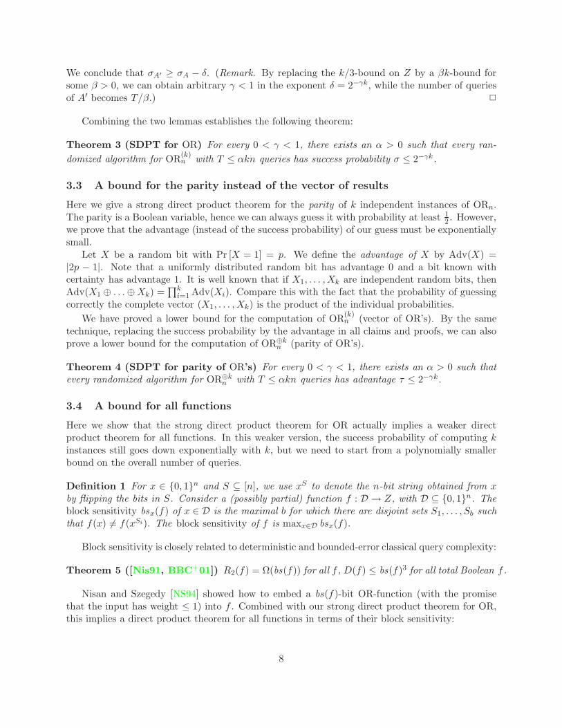
Combining the two lemmas establishes the following theorem:

Theorem 3 (SDPT for OR) For every 0 < γ < 1, there exists an α > 0 such that every ran-

domized algorithm for OR(k)n with T ≤ αkn queries has success probability σ ≤ 2−γk.

3.3 A bound for the parity instead of the vector of results

Here we give a strong direct product theorem for the parity of k independent instances of ORn.The parity is a Boolean variable, hence we can always guess it with probability at least 1

2 . However,we prove that the advantage (instead of the success probability) of our guess must be exponentiallysmall.

Let X be a random bit with Pr [X = 1] = p. We define the advantage of X by Adv(X) =|2p − 1|. Note that a uniformly distributed random bit has advantage 0 and a bit known withcertainty has advantage 1. It is well known that if X1, . . . ,Xk are independent random bits, thenAdv(X1 ⊕ . . . ⊕ Xk) =

∏ki=1 Adv(Xi). Compare this with the fact that the probability of guessing

correctly the complete vector (X1, . . . ,Xk) is the product of the individual probabilities.

We have proved a lower bound for the computation of OR(k)n (vector of OR’s). By the same

technique, replacing the success probability by the advantage in all claims and proofs, we can alsoprove a lower bound for the computation of OR⊕k

n (parity of OR’s).

Theorem 4 (SDPT for parity of OR’s) For every 0 < γ < 1, there exists an α > 0 such thatevery randomized algorithm for OR⊕k

n with T ≤ αkn queries has advantage τ ≤ 2−γk.

3.4 A bound for all functions

Here we show that the strong direct product theorem for OR actually implies a weaker directproduct theorem for all functions. In this weaker version, the success probability of computing kinstances still goes down exponentially with k, but we need to start from a polynomially smallerbound on the overall number of queries.

Definition 1 For x ∈ 0, 1n and S ⊆ [n], we use xS to denote the n-bit string obtained from xby flipping the bits in S. Consider a (possibly partial) function f : D → Z, with D ⊆ 0, 1n. Theblock sensitivity bsx(f) of x ∈ D is the maximal b for which there are disjoint sets S1, . . . , Sb suchthat f(x) 6= f(xSi). The block sensitivity of f is maxx∈D bsx(f).

Block sensitivity is closely related to deterministic and bounded-error classical query complexity:

Theorem 5 ([Nis91, BBC+01]) R2(f) = Ω(bs(f)) for all f , D(f) ≤ bs(f)3 for all total Boolean f .

Nisan and Szegedy [NS94] showed how to embed a bs(f)-bit OR-function (with the promisethat the input has weight ≤ 1) into f . Combined with our strong direct product theorem for OR,this implies a direct product theorem for all functions in terms of their block sensitivity:

8

Theorem 6 For every 0 < γ < 1, there exists an α > 0 such that for every f , every classicalalgorithm for f (k) with T ≤ αkbs(f) queries has success probability σ ≤ 2−γk.

This is optimal whenever R2(f) = Θ(bs(f)), which is the case for most functions. For totalfunctions, the gap between R2(f) and bs(f) is not more than cubic, hence

Corollary 7 For every 0 < γ < 1, there exists an α > 0 such that for every total Boolean f , everyclassical algorithm for f (k) with T ≤ αkR2(f)1/3 queries has success probability σ ≤ 2−γk.

4 Strong Direct Product Theorem for Quantum Queries

In this section we prove a strong direct product theorem for quantum algorithms computing kindependent instances of OR. Our proof relies on the polynomial method of [BBC+01].

4.1 Bounds on polynomials

We use three results about polynomials, also used in [BCWZ99]. The first is by Coppersmith andRivlin [CR92, p. 980] and gives a general bound for polynomials bounded by 1 at integer points:

Theorem 8 (Coppersmith & Rivlin [CR92]) Every polynomial p of degree d ≤ n that hasabsolute value

|p(i)| ≤ 1 for all integers i ∈ [0, n],

satisfies|p(x)| < aebd2/n for all real x ∈ [0, n],

where a, b > 0 are universal constants (no explicit values for a and b are given in [CR92]).

The other two results concern the Chebyshev polynomials Td, defined as in [Riv90]:

Td(x) =1

2

(

(

x +√

x2 − 1)d

+(

x −√

x2 − 1)d)

.

Td has degree d and its absolute value |Td(x)| is bounded by 1 if x ∈ [−1, 1]. On the interval [1,∞),Td exceeds all others polynomials with those two properties ([Riv90, p.108] and [Pat92, Fact 2]):

Theorem 9 If q is a polynomial of degree d such that |q(x)| ≤ 1 for all x ∈ [−1, 1] then |q(x)| ≤|Td(x)| for all x ≥ 1.

Paturi [Pat92, before Fact 2] proved

Lemma 10 (Paturi [Pat92]) Td(1 + µ) ≤ e2d√

2µ+µ2

for all µ ≥ 0.

Proof. For x = 1 + µ: Td(x) ≤ (x +√

x2 − 1)d = (1 + µ +√

2µ + µ2)d ≤ (1 + 2√

2µ + µ2)d ≤e2d

√2µ+µ2

(using that 1 + z ≤ ez for all real z). 2

9

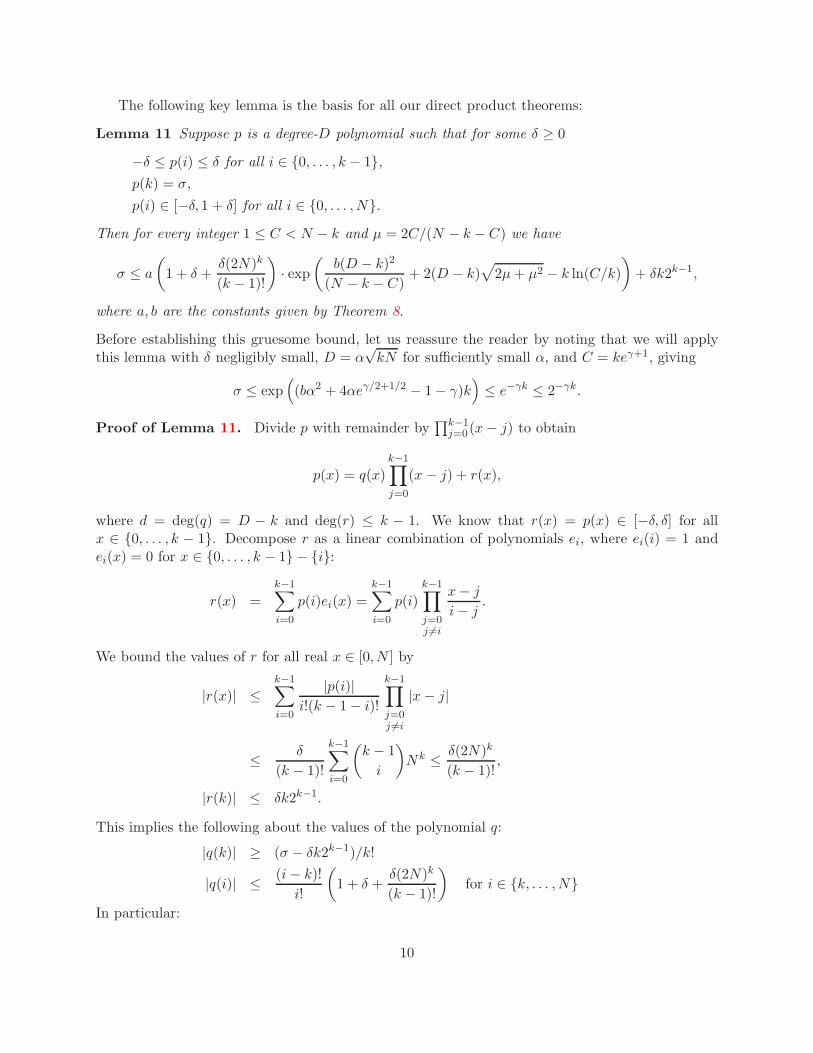
The following key lemma is the basis for all our direct product theorems:

Lemma 11 Suppose p is a degree-D polynomial such that for some δ ≥ 0

−δ ≤ p(i) ≤ δ for all i ∈ 0, . . . , k − 1,p(k) = σ,

p(i) ∈ [−δ, 1 + δ] for all i ∈ 0, . . . , N.Then for every integer 1 ≤ C < N − k and µ = 2C/(N − k − C) we have

σ ≤ a

(

1 + δ +δ(2N)k

(k − 1)!

)

· exp

(

b(D − k)2

(N − k − C)+ 2(D − k)

√

2µ + µ2 − k ln(C/k)

)

+ δk2k−1,

where a, b are the constants given by Theorem 8.

Before establishing this gruesome bound, let us reassure the reader by noting that we will applythis lemma with δ negligibly small, D = α

√kN for sufficiently small α, and C = keγ+1, giving

σ ≤ exp(

(bα2 + 4αeγ/2+1/2 − 1 − γ)k)

≤ e−γk ≤ 2−γk.

Proof of Lemma 11. Divide p with remainder by∏k−1

j=0(x − j) to obtain

p(x) = q(x)k−1∏

j=0

(x − j) + r(x),

where d = deg(q) = D − k and deg(r) ≤ k − 1. We know that r(x) = p(x) ∈ [−δ, δ] for allx ∈ 0, . . . , k − 1. Decompose r as a linear combination of polynomials ei, where ei(i) = 1 andei(x) = 0 for x ∈ 0, . . . , k − 1 − i:

r(x) =

k−1∑

i=0

p(i)ei(x) =

k−1∑

i=0

p(i)

k−1∏

j=0j 6=i

x − j

i − j.

We bound the values of r for all real x ∈ [0, N ] by

|r(x)| ≤k−1∑

i=0

|p(i)|i!(k − 1 − i)!

k−1∏

j=0j 6=i

|x − j|

≤ δ

(k − 1)!

k−1∑

i=0

(

k − 1

i

)

Nk ≤ δ(2N)k

(k − 1)!,

|r(k)| ≤ δk2k−1.

This implies the following about the values of the polynomial q:

|q(k)| ≥ (σ − δk2k−1)/k!

|q(i)| ≤ (i − k)!

i!

(

1 + δ +δ(2N)k

(k − 1)!

)

for i ∈ k, . . . ,N

In particular:

10

|q(i)| ≤ C−k

(

1 + δ +δ(2N)k

(k − 1)!

)

= A for i ∈ k + C, . . . ,N

Theorem 8 implies that there are constants a, b > 0 such that

|q(x)| ≤ A · aebd2/(N−k−C) = B for all real x ∈ [k + C,N ].

We now divide q by B to normalize it, and rescale the interval [k+C,N ] to [1,−1] to get a degree-dpolynomial t satisfying

|t(x)| ≤ 1 for all x ∈ [−1, 1]

t(1 + µ) = q(k)/B for µ = 2C/(N − k − C)

Since t cannot grow faster than the degree-d Chebyshev polynomial, we get

t(1 + µ) ≤ Td(1 + µ) ≤ e2d√

2µ+µ2

.

Combining our upper and lower bounds on t(1 + µ), we obtain

(σ − δk2k−1)/k!

C−k(

1 + δ + δ(2N)k

(k−1)!

)

aebd2/(N−k−C)≤ e2d

√2µ+µ2

.

Rearranging gives the bound. 2

4.2 Consequences for quantum algorithms

The previous result about polynomials implies a strong tradeoff between queries and success prob-ability for quantum algorithms that have to find k ones in an N -bit input. A k-threshold algorithmwith success probability σ is an algorithm on N -bit input x, that outputs 0 with certainty if |x| < k,and outputs 1 with probability at least σ if |x| = k.

Theorem 12 For every γ > 0, there exists an α > 0 such that every quantum k-threshold algorithmwith T ≤ α

√kN queries has success probability σ ≤ 2−γk.

Proof. Fix γ > 0 and consider a T -query k-threshold algorithm. By [BBC+01], its acceptanceprobability is an N -variate polynomial of degree D ≤ 2T ≤ 2α

√kN and can be symmetrized to a

single-variate polynomial p with the properties

p(i) = 0 if i ∈ 0, . . . , k − 1p(k) ≥ σp(i) ∈ [0, 1] for all i ∈ 0, . . . , N

Choosing α > 0 sufficiently small and δ = 0, the result follows from Lemma 11. 2

This implies a strong direct product theorem for k instances of the n-bit search problem:

Theorem 13 (SQDPT for Search) For every γ > 0, there exists an α > 0 such that every

quantum algorithm for Search(k)n with T ≤ αk

√n queries has success probability σ ≤ 2−γk.

11

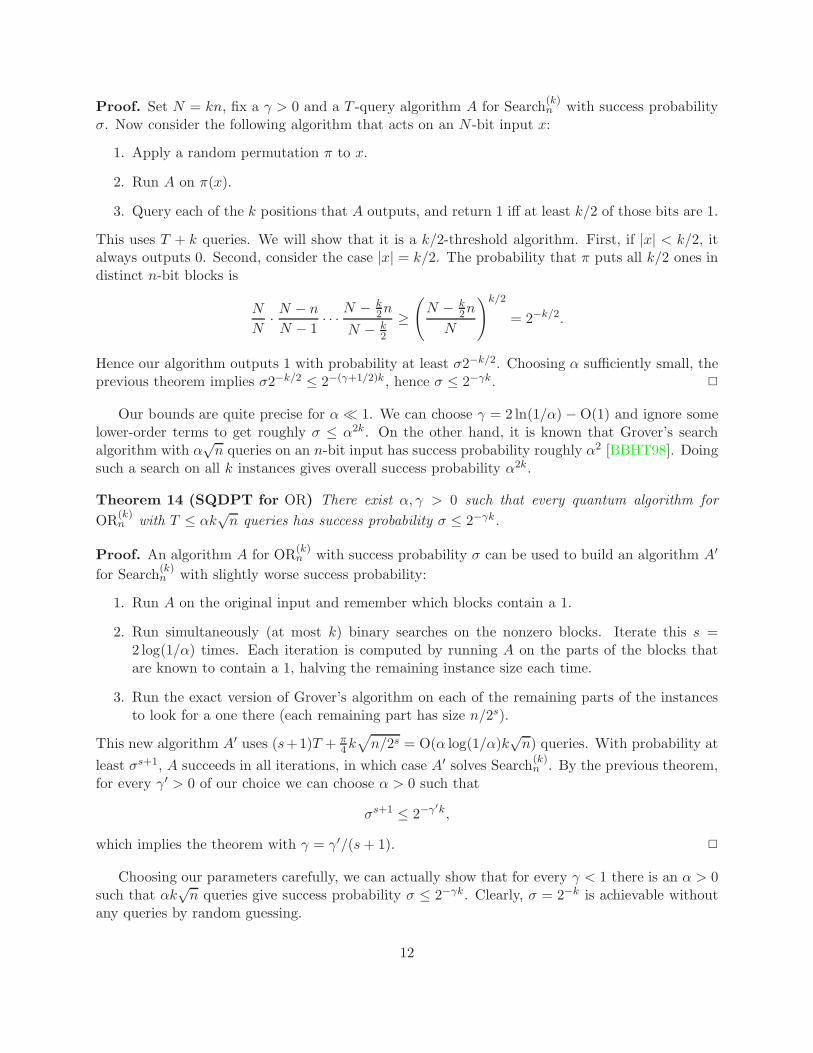
Proof. Set N = kn, fix a γ > 0 and a T -query algorithm A for Search(k)n with success probability

σ. Now consider the following algorithm that acts on an N -bit input x:

1. Apply a random permutation π to x.

2. Run A on π(x).

3. Query each of the k positions that A outputs, and return 1 iff at least k/2 of those bits are 1.

This uses T + k queries. We will show that it is a k/2-threshold algorithm. First, if |x| < k/2, italways outputs 0. Second, consider the case |x| = k/2. The probability that π puts all k/2 ones indistinct n-bit blocks is

N

N· N − n

N − 1· · · N − k

2n

N − k2

≥(

N − k2n

N

)k/2

= 2−k/2.

Hence our algorithm outputs 1 with probability at least σ2−k/2. Choosing α sufficiently small, theprevious theorem implies σ2−k/2 ≤ 2−(γ+1/2)k , hence σ ≤ 2−γk. 2

Our bounds are quite precise for α ≪ 1. We can choose γ = 2 ln(1/α) − O(1) and ignore somelower-order terms to get roughly σ ≤ α2k. On the other hand, it is known that Grover’s searchalgorithm with α

√n queries on an n-bit input has success probability roughly α2 [BBHT98]. Doing

such a search on all k instances gives overall success probability α2k.

Theorem 14 (SQDPT for OR) There exist α, γ > 0 such that every quantum algorithm for

OR(k)n with T ≤ αk

√n queries has success probability σ ≤ 2−γk.

Proof. An algorithm A for OR(k)n with success probability σ can be used to build an algorithm A′

for Search(k)n with slightly worse success probability:

1. Run A on the original input and remember which blocks contain a 1.

2. Run simultaneously (at most k) binary searches on the nonzero blocks. Iterate this s =2 log(1/α) times. Each iteration is computed by running A on the parts of the blocks thatare known to contain a 1, halving the remaining instance size each time.

3. Run the exact version of Grover’s algorithm on each of the remaining parts of the instancesto look for a one there (each remaining part has size n/2s).

This new algorithm A′ uses (s+1)T + π4 k√

n/2s = O(α log(1/α)k√

n) queries. With probability at

least σs+1, A succeeds in all iterations, in which case A′ solves Search(k)n . By the previous theorem,

for every γ′ > 0 of our choice we can choose α > 0 such that

σs+1 ≤ 2−γ′k,

which implies the theorem with γ = γ′/(s + 1). 2

Choosing our parameters carefully, we can actually show that for every γ < 1 there is an α > 0such that αk

√n queries give success probability σ ≤ 2−γk. Clearly, σ = 2−k is achievable without

any queries by random guessing.

12

4.3 A bound for all functions

As in Section 3.4, we can extend the strong direct product theorem for OR to a slightly weakertheorem for all total functions. Block sensitivity is closely related to bounded-error quantum querycomplexity:

Theorem 15 ([BBC+01]) Q2(f) = Ω(

√

bs(f))

for all f , D(f) ≤ bs(f)3 for all total Boolean f .

By embedding an OR of size bs(f) in f , we obtain

Theorem 16 There exist α, γ > 0 such that for every f , every quantum algorithm for f (k) withT ≤ αk

√

bs(f) queries has success probability σ ≤ 2−γk.

This is close to optimal whenever Q2(f) = Θ(

√

bs(f))

. For total functions, the gap between

Q2(f) and√

bs(f) is no more than a 6th power, hence

Corollary 17 There exist α, γ > 0 such that for every total Boolean f , every quantum algorithmfor f (k) with T ≤ αkQ2(f)1/6 queries has success probability σ ≤ 2−γk.

5 Strong Direct Product Theorem for Quantum Communication

In this section we establish a strong direct product theorem for quantum communication complexity,specifically for protocols that compute k independent instances of the Disjointness problem. Ourproof relies crucially on the beautiful technique that Razborov introduced to establish a lower boundon the quantum communication complexity of (one instance of) Disjointness [Raz03]. It allows usto translate a quantum communication protocol to a single-variate polynomial that represents,roughly speaking, the protocol’s acceptance probability as a function of the size of the intersectionof x and y. Once we have this polynomial, the results from Section 4.1 suffice to establish a strongdirect product theorem.

5.1 Razborov’s technique

Razborov’s technique relies on the following linear algebraic notions. The operator norm ‖ A ‖ ofa matrix A is its largest singular value σ1. The trace inner product between A and B is 〈A,B〉 =Tr(A∗B). The trace norm is ‖ A ‖tr = max|〈A,B〉| : ‖ B ‖ = 1 =

∑

i σi. The Frobenius norm is

‖ A ‖F =√

∑

ij |Aij |2 =√

∑

i σ2i . The following lemma is implicit in Razborov’s paper.

Lemma 18 Consider a Q-qubit quantum communication protocol on N -bit inputs x and y, withacceptance probabilities denoted by P (x, y). Define P (i) = E|x|=|y|=N/4,|x∧y|=i|[P (x, y)], where theexpectation is taken uniformly over all x, y that each have weight N/4 and that have intersection i.For every d ≤ N/4 there exists a degree-d polynomial q such that |P (i) − q(i)| ≤ 2−d/4+2Q for alli ∈ 0, . . . , N/8.

Proof. We only consider the N =( NN/4

)

strings of weight N/4. Let P denote the N ×N matrix

of the acceptance probabilities on these inputs. We know from Yao and Kremer [Yao93, Kre95]that we can decompose P as a matrix product P = AB, where A is an N × 22Q−2 matrix with

13

each entry at most 1 in absolute value, and similarly for B. Note that ‖ A ‖F , ‖ B ‖F ≤√N22Q−2.

Using Holder’s inequality we have:

‖ P ‖tr ≤ ‖ A ‖F · ‖ B ‖F ≤ N22Q−2.

Let µi denote the N ×N matrix corresponding to the uniform probability distribution on (x, y) :|x∧y| = i. These “combinatorial matrices” have been well studied [Knu03]. Note that 〈P, µi〉 is theexpected acceptance probability P (i) of the protocol under that distribution. One can show that thedifferent µi commute, so they have the same eigenspaces E0, . . . , EN/4 and can be simultaneously

diagonalized by some orthogonal matrix U . For t ∈ 0, . . . , N/4, let (UPUT )t denote the block ofUPUT corresponding to Et, and at = Tr((UPUT )t) be its trace. Then we have

N/4∑

t=0

|at| ≤N∑

j=1

∣

∣(UPUT )jj∣

∣ ≤ ‖ UPUT ‖tr = ‖ P ‖tr ≤ N22Q−2,

where the second inequality is a property of the trace norm.Let λit be the eigenvalue of µi in eigenspace Et. It is known [Raz03, Section 5.3] that λit is a

degree-t polynomial in i, and that |λit| ≤ 2−t/4/N for i ≤ N/8 (the factor 1/4 in the exponent isimplicit in Razborov’s paper). Consider the high-degree polynomial p defined by

p(i) =

N/4∑

t=0

atλit.

This satisfies

p(i) =

N/4∑

t=0

Tr((UPUT )t)λit = 〈UPUT , UµiUT 〉 = 〈P, µi〉 = P (i).

Let q be the degree-d polynomial obtained by removing the high-degree parts of p:

q(i) =

d∑

t=0

atλit.

Then P and q are close on all integers i between 0 and N/8:

|P (i) − q(i)| = |p(i) − q(i)| =

∣

∣

∣

∣

∣

∣

N/4∑

t=d+1

atλit

∣

∣

∣

∣

∣

∣

≤ 2−d/4

N

N/4∑

t=0

|at| ≤ 2−d/4+2Q.

2

5.2 Consequences for quantum protocols

Combining Razborov’s technique with our polynomial bounds we can prove

Theorem 19 (SQDPT for Disjointness) There exist α, γ > 0 such that every quantum protocol

for DISJ(k)n with Q ≤ αk

√n qubits of communication has success probability p ≤ 2−γk.

14

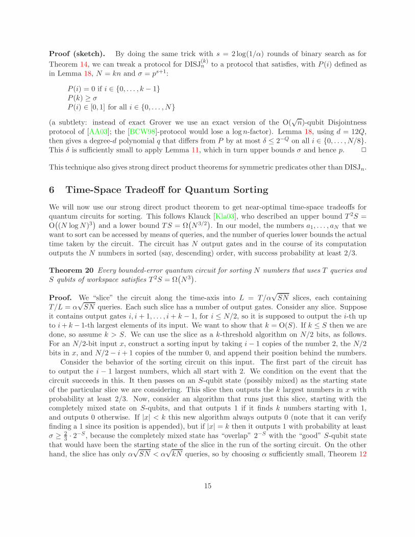
Proof (sketch). By doing the same trick with s = 2 log(1/α) rounds of binary search as for

Theorem 14, we can tweak a protocol for DISJ(k)n to a protocol that satisfies, with P (i) defined as

in Lemma 18, N = kn and σ = ps+1:

P (i) = 0 if i ∈ 0, . . . , k − 1P (k) ≥ σP (i) ∈ [0, 1] for all i ∈ 0, . . . , N

(a subtlety: instead of exact Grover we use an exact version of the O(√

n)-qubit Disjointnessprotocol of [AA03]; the [BCW98]-protocol would lose a log n-factor). Lemma 18, using d = 12Q,then gives a degree-d polynomial q that differs from P by at most δ ≤ 2−Q on all i ∈ 0, . . . , N/8.This δ is sufficiently small to apply Lemma 11, which in turn upper bounds σ and hence p. 2

This technique also gives strong direct product theorems for symmetric predicates other than DISJn.

6 Time-Space Tradeoff for Quantum Sorting

We will now use our strong direct product theorem to get near-optimal time-space tradeoffs forquantum circuits for sorting. This follows Klauck [Kla03], who described an upper bound T 2S =O(

(N log N)3)

and a lower bound TS = Ω(

N3/2)

. In our model, the numbers a1, . . . , aN that wewant to sort can be accessed by means of queries, and the number of queries lower bounds the actualtime taken by the circuit. The circuit has N output gates and in the course of its computationoutputs the N numbers in sorted (say, descending) order, with success probability at least 2/3.

Theorem 20 Every bounded-error quantum circuit for sorting N numbers that uses T queries andS qubits of workspace satisfies T 2S = Ω

(

N3)

.

Proof. We “slice” the circuit along the time-axis into L = T/α√

SN slices, each containingT/L = α

√SN queries. Each such slice has a number of output gates. Consider any slice. Suppose

it contains output gates i, i + 1, . . . , i + k − 1, for i ≤ N/2, so it is supposed to output the i-th upto i + k − 1-th largest elements of its input. We want to show that k = O(S). If k ≤ S then we aredone, so assume k > S. We can use the slice as a k-threshold algorithm on N/2 bits, as follows.For an N/2-bit input x, construct a sorting input by taking i − 1 copies of the number 2, the N/2bits in x, and N/2 − i + 1 copies of the number 0, and append their position behind the numbers.

Consider the behavior of the sorting circuit on this input. The first part of the circuit hasto output the i − 1 largest numbers, which all start with 2. We condition on the event that thecircuit succeeds in this. It then passes on an S-qubit state (possibly mixed) as the starting stateof the particular slice we are considering. This slice then outputs the k largest numbers in x withprobability at least 2/3. Now, consider an algorithm that runs just this slice, starting with thecompletely mixed state on S-qubits, and that outputs 1 if it finds k numbers starting with 1,and outputs 0 otherwise. If |x| < k this new algorithm always outputs 0 (note that it can verifyfinding a 1 since its position is appended), but if |x| = k then it outputs 1 with probability at leastσ ≥ 2

3 · 2−S , because the completely mixed state has “overlap” 2−S with the “good” S-qubit statethat would have been the starting state of the slice in the run of the sorting circuit. On the otherhand, the slice has only α

√SN < α

√kN queries, so by choosing α sufficiently small, Theorem 12

15

implies σ ≤ 2−Ω(k). Combining our upper and lower bounds on σ gives k = O(S). Thus we need

L = Ω(N/S) slices, so T = Lα√

SN = Ω(

N3/2/√

S)

. 2

As mentioned, our tradeoff is achievable up to polylog factors [Kla03]. Interestingly, the near-optimal algorithm uses only a polylogarithmic number of qubits and otherwise just classical memory.For simplicity we have shown the lower bound for the case when the outputs have to be made intheir natural ordering only, but we can show the same lower bound for any ordering of the outputsthat does not depend on the input using a slightly different proof.

7 Time-Space Tradeoffs for Boolean Matrix Products

First we show a lower bound on the time-space tradeoff for Boolean matrix-vector multiplicationon classical machines.

Theorem 21 There is a matrix A such that every classical bounded-error circuit that computes theBoolean matrix-vector product Ab with T queries and space S = o(N/ log N) satisfies TS = Ω

(

N2)

.

The bound is tight if T measures queries to the input.

Proof. Fix k = O(S) large enough. First we have to find a hard matrix A. We pick A randomly bysetting N/(2k) random positions in each row to 1. We want to show that with positive probabilityfor all sets of k rows A[i1], . . . , A[ik] many of the rows A[ij ] contain at least N/(6k) ones that arenot ones in any of the k − 1 other rows.

This probability can be bounded as follows. We will treat the rows as subsets of 1, . . . , N. Arow A[j] is called bad with respect to k−1 other rows A[i1], . . . , A[ik−1], if |A[j]−∪ℓA[iℓ]| ≤ N/(6k).For fixed i1, . . . , ik−1, the probability that some A[j] is bad with respect to the k − 1 other rowsis at most e−Ω(N/k) by the Chernoff bound and the fact that k rows can together contain at mostN/2 elements. Since k = o(N/ log N) we may assume this probability is at most 1/N10.

Now fix any set I = i1, . . . , ik. The probability that for j ∈ I it holds that A[j] is bad withrespect to the other rows is at most 1/N10, and this also holds, if we condition on the event thatsome other rows are bad, since this condition makes it only less probable that another row is alsobad. So for any fixed J ⊂ I of size k/2 the probability that all rows in J are bad is at most N−5k,and the probability that there exists such J is at most

(

k

k/2

)

N−5k.

Furthermore the probability that there is a set I of k rows for which k/2 are bad is at most(

N

k

)(

k

k/2

)

N−5k < 1.

So there is an A as required and we may fix one.Now suppose we are given a circuit with space S that computes the Boolean product between

the rows of A and b in some order. We again proceed by “slicing” the circuit into L = T/αNslices, each containing T/L = αN queries. Each such slice has a number of output gates. Considerany slice. Suppose it contains output gates i1 < . . . < ik ≤ N/2, so it is supposed to output∨N

ℓ=1 (A[ij , ℓ] ∧ bℓ) for all ij with 1 ≤ j ≤ k.

16

Such a slice starts on a classical value of the “memory” of the circuit, which is in generala probability distribution on S bits (if the circuit is randomized). We replace this probabilitydistribution by the uniform distribution on the possible values of S bits. If the original circuitsucceeds in computing the function correctly with probability at least 1/2, then so does the circuitslice with its outputs, and replacing the initial value of the memory by a uniformly random onedecreases the success probability to no less than (1/2) · 1/2S .

If we now show that any classical circuit with αN queries that produces the outputs i1, . . . , ikcan succeed only with exponentially small probability in k, we get that k = O(S), and hence(T/αN) · O(S) ≥ N , which gives the claimed lower bound for the time-space tradeoff.

Each set of k outputs corresponds to k rows of A, which contain N/(2k) ones each. Thanksto the construction of A there are k/2 rows among these, such that N/(6k) of the ones in eachsuch row are in position where none of the other contains a one. So we get k/2 sets of N/(6k)positions that are unique to each of the k/2 rows. The inputs for b will be restricted to contain onesonly at these positions, and so the algorithm naturally has to solve k/2 independent OR problemson n = N/(6k) bits each. By Theorem 3, this is only possible with αN queries if the successprobability is exponentially small in k. 2

An absolutely analogous construction can be done in the quantum case. Using circuit slices oflength α

√NS we can prove:

Theorem 22 There is a matrix A such that every quantum bounded-error circuit that computes theBoolean matrix-vector product Ab with T queries and space S = o(N/ log N) satisfies T 2S = Ω

(

N3)

.

Note that this is tight within a logarithmic factor (needed to improve the success probabilityof Grover search).

Theorem 23 Every classical bounded-error circuit that computes the Boolean matrix product ABwith T queries and space S satisfies TS = Ω

(

N3)

.

While this is near-optimal for small S, it is probably not tight for large S, a likely tighttradeoff being T 2S = Ω

(

N6)

. It is also no improvement compared to Abrahamson’s average-casebounds [Abr90].

Proof. Suppose that S = o(N), otherwise the bound is trivial, since time N2 is always needed.We can proceed similar to the proof of Theorem 21. We slice the circuit so that each slice has onlyαN queries. Suppose a slice makes k outputs. We are going to restrict the inputs to get a directproduct problem with k instances of size N/k each, hence a slice with αN queries has exponentiallysmall success probability in k and can thus produce only O(S) outputs. Since the overall numberof outputs is N2 we get the tradeoff TS = Ω

(

N3)

.Suppose a circuit slice makes k outputs, where an output labeled (i, j) needs to produce the

vector product of the ith row A[i] of A and the jth column B[j] of B. We may partition the set1, . . . , N into k mutually disjoint subsets U(i, j) of size N/k, each associated to an output (i, j).

Assume that there are ℓ outputs (i, j1), . . . , (i, jℓ) involving A[i]. Each such output is associatedto a subset U(i, jt), and we set A[i] to zero on all positions that are not in any of these subsets,and to one on all positions that are in one of these. When there are ℓ outputs (i1, j), . . . , (iℓ, j)involving B[j], we set B[j] to zero on all positions that are not in any of the corresponding subsets,and allow the inputs to be arbitrary on the other positions.

17

If the circuit computes on these restricted inputs, it actually has to compute k instances of ORof size n = N/k in B, for it is true that A[i] and B[j] contain a single block of size N/k in whichA[i] contains only ones, and B[j] “free” input bits, if and only if (i, j) is one of the k outputs.Hence the strong direct product theorem is applicable. 2

The application to the quantum case is analogous.

Theorem 24 Every quantum bounded-error circuit that computes the Boolean matrix product ABwith T queries and space S satisfies T 2S = Ω

(

N5)

.

If S = O(log N), then N2 applications of Grover can compute AB with T = O(

N2.5 log N)

. Henceour tradeoff is near-optimal for small S. We do not know whether it is optimal for large S.

8 Quantum Communication-Space Tradeoffs for Matrix Products

In this section we use the strong direct product result for quantum communication (Theorem 19)to prove communication-space tradeoffs. We later show that these are close to optimal.

Theorem 25 Every quantum bounded-error protocol in which Alice and Bob have bounded spaceS and that computes the Boolean matrix-vector product, satisfies C2S = Ω

(

N3)

.

Proof. In a protocol, Alice receives a matrix A, and Bob a vector b as inputs. Given a circuitthat multiplies these with communication C and space S, we again proceed to slice it. Thistime, however, a slice contains a limited amount of communication. Recall that in communicatingquantum circuits the communication corresponds to wires carrying qubits that cross between Alice’sand Bob’s circuits. Hence we may cut the circuit after α

√NS qubits have been communicated

and so on. Overall there are C/α√

NS circuit slices. Each starts with an initial state that maybe replaced by the completely mixed state at the cost of decreasing the success probability to(1/2)·1/2S . We want to employ the direct product theorem for quantum communication complexityto show that a protocol with the given communication has success probability at most exponentiallysmall in the number of outputs it produces, and so a slice can produce at most O(S) outputs.Combining these bounds with the fact that N outputs have to be produced gives the tradeoff.

To use the direct product theorem we restrict the inputs in the following way: Suppose aprotocol makes k outputs. We partition the vector b into k blocks of size N/k, and each blockis assigned to one of the k rows of A for which an output is made. This row is made to containzeroes outside of the positions belonging to its block, and hence we arrive at a problem whereDisjointness has to be computed on k instances of size N/k. With communication α

√kN , the

success probability must be exponentially small in k due to Theorem 19. Hence k = O(S) is anupper bound on the number of outputs produced. 2

Theorem 26 Every quantum bounded-error protocol in which Alice and Bob have bounded spaceS and that computes the Boolean matrix product, satisfies C2S = Ω

(

N5)

.

Proof. The proof uses the same slicing approach as in the other tradeoff results. Note that we canassume that S = o(N), since otherwise the bound is trivial. Each slice contains communication

18

α√

NS, and as before a direct product result showing that k outputs can be computed only withsuccess probability exponentially small in k leads to the conclusion that a slice can only computeO(S) outputs. Therefore (C/α

√NS) · O(S) ≥ N2, and we are done.

Consider a protocol with α√

NS qubits of communication. We partition the universe 1, . . . , Nof the Disjointness problems to be computed into k mutually disjoint subsets U(i, j) of size N/k,each associated to an output (i, j), which in turn corresponds to a row/column pair A[i], B[j] inthe input matrices A and B. Assume that there are ℓ outputs (i, j1), . . . , (i, jℓ) involving A[i]. Eachoutput is associated to a subset of the universe U(i, jt), and we set A[i] to zero on all positions thatare not in one of these subsets. Then we proceed analogously with the columns of B.

If the protocol computes on these restricted inputs, it has to solve k instances of Disjointnessof size n = N/k each, since A[i] and B[j] contain a single block of size N/k in which both are notset to 0 if and only if (i, j) is one of the k outputs. Hence Theorem 19 is applicable. 2

We now want to show that these tradeoffs are not too far from optimal.

Theorem 27 There is a quantum bounded-error protocol with space S that computes the Booleanproduct between a matrix and a vector within communication C = O((N3/2 log2 N)/

√S).

There is a quantum bounded-error protocol with space S that computes the Boolean productbetween two matrices within communication C = O((N5/2 log2 N)/

√S).

Proof. We begin by showing a protocol for the following scenario: Alice gets S N -bit vectorsx1, . . . , xS , Bob gets an N -vector vector y, and they want to compute the S Boolean inner productsbetween these vectors. The protocol uses space O(S).

In the following, we interpret Boolean vectors as sets. The main idea is that Alice can use theunion z of the xi and then Alice and Bob can find an element in the intersection of z and y using theprotocol for the Disjointness problem described in [BCW98]. Alice then marks all xi that containthis element and removes them from z.

A problem with this approach is that Alice cannot store z explicitly, since it might containmuch more than S elements. Alice may, however, store the indices of those sets xi for which anelement in the intersection of xi and y has already been found, in an array of length S. This arrayand the input given as an oracle work as an implicit representation of z.

Now suppose at some point during the protocol the intersection of z and y has size k. ThenAlice and Bob can find one element in this intersection within O(

√

N/k) rounds of communicationin which O(log N) qubits are exchanged each. Furthermore in O(

√Nk) rounds all elements in

the intersection can be found. So if k ≤ S, then all elements are found within communicationO(

√NS log N) and the problem can be solved completely. On the other hand, if k ≥ S, finding

one element costs O(√

N/S log N), but finding such an element removes at least one xi from z,and hence this has to be done at most S times, giving the same overall communication bound.

It is not hard to see that this process can be implemented with space O(S). The protocol from[BCW98] is a distributed Grover search that itself uses only space O(log N). Bob can work as inthis protocol. For each search, Alice has to start with a superposition over all indices in z. Thissuperposition can be computed from her oracle and her array. In each step she has to apply theGrover iteration. This can also be implemented from these two resources.

To get a protocol for matrix-vector product, the above procedure is repeated N/S times, hencethe communication is O((N/S) ·

√NS log2 N), where one logarithmic factor stems from improving

success probability to 1/poly(N).

19

For the product of two matrices, the matrix-vector protocol may be repeated N times. 2

These near-optimal protocols use only O(log N) “real” qubits, and otherwise just classical memory.

9 Open Problems

We mention some open problems. The first is to determine tight time-space tradeoffs for Booleanmatrix product on both classical and quantum computers. Second, regarding communication-spacetradeoffs for Boolean matrix-vector and matrix product, we did not prove any classical bounds thatwere better than our quantum bounds. Klauck [Kla04] recently proved classical tradeoffs CS2 =Ω(

N3)

and CS2 = Ω(

N2)

for Boolean matrix product and matrix-vector product, respectively, bymeans of a weak direct product theorem for Disjointness. A classical strong direct product theoremfor Disjointness would imply optimal tradeoffs, but we do not know how to prove this at the moment.Finally, it would be interesting to get any lower bounds on time-space or communication-spacetradeoffs for decision problems in the quantum case, for example for Element Distinctness [BDH+01,Amb03] or the verification of matrix multiplication [BS04].

Acknowledgments

We thank Scott Aaronson for email discussions about the evolving results in his [Aar04] thatmotivated some of our proofs, and Harry Buhrman for useful discussions.

References

[AA03] S. Aaronson and A. Ambainis. Quantum search of spatial regions. In Proceedings of44th IEEE FOCS, pages 200–209, 2003. quant-ph/0303041.

[Aar04] S. Aaronson. Limitations of quantum advice and one-way communication. In Pro-ceedings of 19th IEEE Conference on Computational Complexity, pages 320–332, 2004.quant-ph/0402095.

[Abr90] K. Abrahamson. A time-space tradeoff for Boolean matrix multiplication. In Proceed-ings of 31st IEEE FOCS, pages 412–419, 1990.

[Amb03] A. Ambainis. Quantum walk algorithm for element distinctness. quant-ph/0311001, 1Nov 2003.

[BBC+01] R. Beals, H. Buhrman, R. Cleve, M. Mosca, and R. de Wolf. Quantum lower boundsby polynomials. Journal of the ACM, 48(4):778–797, 2001. Earlier version in FOCS’98.quant-ph/9802049.

[BBHT98] M. Boyer, G. Brassard, P. Høyer, and A. Tapp. Tight bounds on quantum searching.Fortschritte der Physik, 46(4–5):493–505, 1998. Earlier version in Physcomp’96. quant-ph/9605034.

[BCW98] H. Buhrman, R. Cleve, and A. Wigderson. Quantum vs. classical communicationand computation. In Proceedings of 30th ACM STOC, pages 63–68, 1998. quant-ph/9802040.

20

[BCWZ99] H. Buhrman, R. Cleve, R. de Wolf, and Ch. Zalka. Bounds for small-error and zero-error quantum algorithms. In Proceedings of 40th IEEE FOCS, pages 358–368, 1999.cs.CC/9904019.

[BDH+01] H. Buhrman, Ch. Durr, M. Heiligman, P. Høyer, F. Magniez, M. Santha, and R. deWolf. Quantum algorithms for element distinctness. In Proceedings of 16th IEEEConference on Computational Complexity, pages 131–137, 2001. quant-ph/0007016.

[Bea91] P. Beame. A general sequential time-space tradeoff for finding unique elements. SIAMJournal on Computing, 20(2):270–277, 1991. Earlier version in STOC’89.

[BFS86] L. Babai, P. Frankl, and J. Simon. Complexity classes in communication complexitytheory. In Proceedings of 27th IEEE FOCS, pages 337–347, 1986.

[BHMT02] G. Brassard, P. Høyer, M. Mosca, and A. Tapp. Quantum amplitude amplificationand estimation. In Quantum Computation and Quantum Information: A MillenniumVolume, volume 305 of AMS Contemporary Mathematics Series, pages 53–74. 2002.quant-ph/0005055.

[BNRW03] H. Buhrman, I. Newman, H. Rohrig, and R. de Wolf. Robust quantum algorithms andpolynomials. quant-ph/0309220, 30 Sep 2003.

[BS04] H. Buhrman and R. Spalek. Quantum verification of matrix products. Unpublishedmanuscript, 2004.

[BTY94] P. Beame, M. Tompa, and P. Yan. Communication-space tradeoffs for unrestricted pro-tocols. SIAM Journal on Computing, 23(3):652–661, 1994. Earlier version in FOCS’90.

[Buh00] H. Buhrman. Quantum computing and communication complexity. EATCS Bulletin,70:131–141, February 2000.

[BW02] H. Buhrman and R. de Wolf. Complexity measures and decision tree complexity: Asurvey. Theoretical Computer Science, 288(1):21–43, 2002.

[CDNT98] R. Cleve, W. van Dam, M. Nielsen, and A. Tapp. Quantum entanglement and thecommunication complexity of the inner product function. In Proceedings of 1st NASAQCQC conference, volume 1509 of Lecture Notes in Computer Science, pages 61–74.Springer, 1998. quant-ph/9708019.

[CR92] D. Coppersmith and T. J. Rivlin. The growth of polynomials bounded at equally spacedpoints. SIAM Journal on Mathematical Analysis, 23(4):970–983, 1992.

[GNW95] O. Goldreich, N. Nisan, and A. Wigderson. On Yao’s XOR lemma. Technical report,ECCC TR–95–050, 1995. Available at http://www.eccc.uni-trier.de/eccc/.

[Gro96] L. K. Grover. A fast quantum mechanical algorithm for database search. In Proceedingsof 28th ACM STOC, pages 212–219, 1996. quant-ph/9605043.

[HW02] P. Høyer and R. de Wolf. Improved quantum communication complexity bounds fordisjointness and equality. In Proceedings of 19th Annual Symposium on TheoreticalAspects of Computer Science (STACS’2002), volume 2285 of Lecture Notes in ComputerScience, pages 299–310. Springer, 2002. quant-ph/0109068.

21

[Kla00] H. Klauck. Quantum communication complexity. In Proceedings of Workshop onBoolean Functions and Applications at 27th ICALP, pages 241–252, 2000. quant-ph/0005032.

[Kla03] H. Klauck. Quantum time-space tradeoffs for sorting. In Proceedings of 35th ACMSTOC, pages 69–76, 2003. quant-ph/0211174.

[Kla04] H. Klauck. Quantum and classical communication-space tradeoffs from rectanglebounds. Unpublished manuscript, 2004.

[KN97] E. Kushilevitz and N. Nisan. Communication Complexity. Cambridge University Press,1997.

[Knu03] D. E. Knuth. Combinatorial matrices. In Selected Papers on Discrete Mathematics,volume 106 of CSLI Lecture Notes. Stanford University, 2003.

[Kre95] I. Kremer. Quantum communication. Master’s thesis, Hebrew University, ComputerScience Department, 1995.

[KS92] B. Kalyanasundaram and G. Schnitger. The probabilistic communication complexity ofset intersection. SIAM Journal on Discrete Mathematics, 5(4):545–557, 1992. Earlierversion in Structures’87.

[LTT92] T.W. Lam, P. Tiwari, and M. Tompa. Trade-offs between communication and space.Journal of Computer and Systems Sciences, 45(3):296–315, 1992. Earlier version inSTOC’89.

[NC00] M. A. Nielsen and I. L. Chuang. Quantum Computation and Quantum Information.Cambridge University Press, 2000.

[Nis91] N. Nisan. CREW PRAMs and decision trees. SIAM Journal on Computing, 20(6):999–1007, 1991. Earlier version in STOC’89.

[NRS94] N. Nisan, S. Rudich, and M. Saks. Products and help bits in decision trees. In Pro-ceedings of 35th FOCS, pages 318–329, 1994.

[NS94] N. Nisan and M. Szegedy. On the degree of Boolean functions as real polynomials.Computational Complexity, 4(4):301–313, 1994. Earlier version in STOC’92.

[Pat92] R. Paturi. On the degree of polynomials that approximate symmetric Boolean functions.In Proceedings of 24th ACM STOC, pages 468–474, 1992.

[PRW97] I. Parnafes, R. Raz, and A. Wigderson. Direct product results and the GCD problem,in old and new communication models. In Proceedings of 29th ACM STOC, pages363–372, 1997.

[Raz92] A. Razborov. On the distributional complexity of disjointness. Theoretical ComputerScience, 106(2):385–390, 1992.

[Raz03] A. Razborov. Quantum communication complexity of symmetric predicates. Izvestiya ofthe Russian Academy of Science, mathematics, 67(1):159–176, 2003. quant-ph/0204025.

22

[Riv90] T. J. Rivlin. Chebyshev Polynomials: From Approximation Theory to Algebra andNumber Theory. Wiley-Interscience, second edition, 1990.

[Sha01] R. Shaltiel. Towards proving strong direct product theorems. In Proceedings of 16thIEEE Conference on Computational Complexity, pages 107–119, 2001.

[Wol02] R. de Wolf. Quantum communication and complexity. Theoretical Computer Science,287(1):337–353, 2002.

[Yao77] A. C-C. Yao. Probabilistic computations: Toward a unified measure of complexity. InProceedings of 18th IEEE FOCS, pages 222–227, 1977.

[Yao82] A. C-C. Yao. Theory and applications of trapdoor functions. In Proceedings of 23rdIEEE FOCS, pages 80–91, 1982.

[Yao93] A. C-C. Yao. Quantum circuit complexity. In Proceedings of 34th IEEE FOCS, pages352–360, 1993.

23